

Ubaldo Garibaldi, Enrico Scalas-Finitary Probabilistic Methods in Econophysics (2010)
343
-
Upload
giovannierario -
Category
Documents
-
view
25 -
download
0
description
Ubaldo Garibaldi, Enrico Scalas-Finitary Probabilistic Methods in Econophysics (2010)
Transcript of Ubaldo Garibaldi, Enrico Scalas-Finitary Probabilistic Methods in Econophysics (2010)

This page intentionally left blank
FINITARY PROBABILISTIC METHODS INECONOPHYSICS
Econophysics applies the methodology of physics to the study of economics.However, whilst physicists have a good understanding of statistical physics, theyare often unfamiliar with recent advances in statistics, including Bayesian and pre-dictive methods. Equally, economists with knowledge of probabilities do not havea background in statistical physics and agent-based models. Proposing a unifiedview for a dynamic probabilistic approach, this book is useful for advanced under-graduate and graduate students as well as researchers in physics, economics andfinance.
The book takes a finitary approach to the subject. It discusses the essentials ofapplied probability, and covers finite Markov chain theory and its applications toreal systems. Each chapter ends with a summary, suggestions for further readingand exercises with solutions at the end of the book.
Ubaldo Garibaldi is First Researcher at the IMEM-CNR, Italy, where heresearches the foundations of probability, statistics and statistical mechanics, andthe application of finite Markov chains to complex systems.
Enrico Scalas is Assistant Professor of Physics at the University of EasternPiedmont, Italy. His research interests are anomalous diffusion and its applica-tions to complex systems, the foundations of statistical mechanics and agent-basedsimulations in physics, finance and economics.

FINITARY PROBABILISTICMETHODS IN ECONOPHYSICS
UBALDO GARIBALDIIMEM-CNR, Italy
ENRICO SCALASUniversity of Eastern Piedmont, Italy

CAMBRIDGE UNIVERSITY PRESSCambridge, New York, Melbourne, Madrid, Cape Town, Singapore,São Paulo, Delhi, Dubai, Tokyo
Cambridge University PressThe Edinburgh Building, Cambridge CB2 8RU, UK
First published in print format
ISBN-13 978-0-521-51559-7
ISBN-13 978-0-511-90205-5
© U. Garibaldi and E. Scalas 2010
2010
Information on this title: www.cambridge.org/9780521515597
This publication is in copyright. Subject to statutory exception and to the provision of relevant collective licensing agreements, no reproduction of any partmay take place without the written permission of Cambridge University Press.
Cambridge University Press has no responsibility for the persistence or accuracy of urls for external or third-party internet websites referred to in this publication, and does not guarantee that any content on such websites is, or will remain, accurate or appropriate.
Published in the United States of America by Cambridge University Press, New York
www.cambridge.org
eBook (NetLibrary)
Hardback
Contents
Foreword page ixAcknowledgements xiii1 Introductory remarks 1
1.1 Early accounts and the birth of mathematical probability 11.2 Laplace and the classical definition of probability 31.3 Frequentism 81.4 Subjectivism, neo-Bayesianism and logicism 101.5 From definitions to interpretations 12Further reading 13References 13
2 Individual and statistical descriptions 152.1 Joint α-descriptions and s-descriptions 152.2 Frequency vector and individual descriptions 182.3 Partitions 192.4 Partial and marginal descriptions 202.5 Exercises 242.6 Summary 24Further reading 25
3 Probability and events 263.1 Elementary descriptions and events 263.2 Decompositions of the sample space 293.3 Remarks on distributions 323.4 Probability assignments 353.5 Remarks on urn models and predictive probabilities 393.6 Appendix: outline of elementary probability theory 423.7 Exercises 543.8 Summary 55Further reading 55References 57
v
vi Contents
4 Finite random variables and stochastic processes 584.1 Finite random variables 584.2 Finite stochastic processes 734.3 Appendix 1: a finite version of de Finetti’s theorem 864.4 Appendix 2: the beta distribution 924.5 Exercises 934.6 Summary 93Further reading 94References 95
5 The Pólya process 965.1 Definition of the Pólya process 965.2 The first moments of the Pólya distribution 1005.3 Label mixing and marginal distributions 1045.4 A consequence of the constraint
∑ni = n 116
5.5 The continuum limits of the multivariate Pólya distribution 1165.6 The fundamental representation theorem for the
Pólya process 1235.7 Exercises 1305.8 Summary 131Further reading 132
6 Time evolution and finite Markov chains 1346.1 From kinematics to Markovian probabilistic dynamics 1346.2 The Ehrenfest urn model 1396.3 Finite Markov chains 1416.4 Convergence to a limiting distribution 1466.5 The invariant distribution 1526.6 Reversibility 1606.7 Exercises 1666.8 Summary 169Further reading 169References 171
7 The Ehrenfest–Brillouin model 1727.1 Merging Ehrenfest-like destructions and
Brillouin-like creations 1727.2 Unary moves 1747.3 From fleas to ants 1777.4 More complicated moves 1807.5 Pólya distribution structures 1817.6 An application to stock price dynamics 1887.7 Exogenous constraints and the most probable
occupation vector 193

Contents vii
7.8 Exercises 2017.9 Summary 201Further reading 202
8 Applications to stylized models in economics 2048.1 A model for random coin exchange 2048.2 The taxation–redistribution model 2128.3 The Aoki–Yoshikawa model for sectoral productivity 2178.4 General remarks on statistical equilibrium in economics 2238.5 Exercises 2258.6 Summary 225Further reading 226References 228
9 Finitary characterization of the Ewens sampling formula 2299.1 Infinite number of categories 2299.2 Finitary derivation of the Ewens sampling formula 2329.3 Cluster number distribution 2389.4 Ewens’ moments and site-label marginals 2409.5 Alternative derivation of the expected number of clusters 2439.6 Sampling and accommodation 2449.7 Markov chains for cluster and site dynamics 2479.8 Marginal cluster dynamics and site dynamics 2509.9 The two-parameter Ewens process 2569.10 Summary 259Further reading 260
10 The Zipf–Simon–Yule process 26210.1 The Ewens sampling formula and firm sizes 26210.2 Hoppe’s vs. Zipf’s urn 26310.3 Expected cluster size dynamics and the Yule distribution 26510.4 Birth and death Simon–Zipf’s process 26910.5 Marginal description of the Simon–Zipf process 27110.6 A formal reversible birth-and-death marginal chain 27410.7 Monte Carlo simulations 27610.8 Continuous limit and diffusions 27910.9 Appendix 1: invariant measure for homogeneous diffusions 28610.10 Summary 287Further reading 288
Appendix 289Solutions to exercises 289
Author index 323Subject index 325

Foreword
The theme of this book is the allocation of n objects (or elements) into g categories(or classes), discussed from several viewpoints. This approach can be traced backto the early work of 24-year-old Ludwig Boltzmann in his first attempt to deriveMaxwell’s distribution of velocity for a perfect gas in probabilistic terms.
Chapter 2 explains how to describe the state of affairs in which for every objectlisted ‘alphabetically’ or in a sampling order, its category is given. We can considerthe descriptions of Chapter 2 as facts (taking place or not), and events as propositions(true or not) about facts (taking place or not). Not everything in the world is known,and what remains is a set of possibilities. For this reason, in Chapter 3, we show howevents can be probabilized and we present the basic probability axioms and theirconsequences. In Chapter 4, the results of the previous two chapters are rephrasedin the powerful language of random variables and stochastic processes.
Even if the problem of allocating n objects into g categories may seem trivial, itturns out that many important problems in statistical physics and some problems ineconomics and finance can be formulated and solved using the methods describedin Chapters 2, 3 and 4. Indeed, the allocation problem is far from trivial. In fact,in the language of the logical approach to probability, traced back to Johnson and,mainly, to Carnap, the individual descriptions and the statistical descriptions are anessential tool to represent possible worlds. A neglected paper written by Brillouinshowed that the celebrated Bose–Einstein, Fermi–Dirac and Maxwell–Boltzmanndistributions of statistical physics are nothing other than particular cases of theone-parameter multivariate accommodation process, where bosons share the samepredictive probability as in Laplace’s succession rule. These are particular instancesof the generalized multivariate Pólya distribution studied in Chapter 5 as a samplingdistribution of the Pólya process. The Pólya process is an n-exchangeable stochasticprocess, whose characterization leads us to discuss Pearson’s fundamental problemof practical statistics, that is, given that a result of an experiment has been observed
ix
What is this book about?
x Foreword
r times out of m trials, what is the probability of observing the result in the next(the (m + 1)th) trial?
Up to Chapter 5, we study the allocation of n objects into g categories eitheras an accommodation process or as a sampling process. The index set of the finiteindividual stochastic processes studied in Chapters 4 and 5 may represent eitherthe name of the objects or their order of appearance in a sampling procedure. Inother words, objects are classified once for all. If time enters and change becomespossible, the simplest probabilistic description of n objects jumping within g cat-egories as time goes by is given in terms of finite Markov chains, which are anextension in several directions of the famous Ehrenfest urn model. This is the sub-ject of Chapter 6. For the class of irreducible Markov chains, those chains in whicheach state can be reached from any other state, there exists a unique invariant dis-tribution, that is a probability distribution over the state space which is not affectedby the time evolution. If the Markov chain is also aperiodic, meaning that the initialconditions are forgotten forever during time evolution, then the invariant distribu-tion is also the equilibrium distribution. This means that, irrespective of the initialconditions, in the long run, the chain is described by its invariant distribution, whichsummarizes all the relevant statistical properties. Moreover, the ergodic problem ofstatistical physics finds a complete solution in the theory of finite Markov chains.For finite, aperiodic and irreducible Markov chains, time averages converge toensemble averages computed according to the invariant (and equilibrium) distri-bution. Incidentally, in this framework, many out-of-equilibrium properties can bederived. The Ehrenfest–Brillouin Markov chain of Chapter 7 encompasses manyuseful models of physics, finance and economics. This is shown not only in Chapter7, but also in Chapter 8, where a detailed review of some recent results of ours ispresented. These models describe a change of category as a sequence of an Ehren-fest destruction (where an element is selected at random and removed from thesystem) followed by a Brillouin creation (where an element re-accommodates inthe system according to a Pólya weight).
The Pólya distribution is the invariant and equilibrium distribution for theEhrenfest–Brillouin Markov chain. In Chapter 9, we study what happens to thePólya distribution and to the Ehrenfest–Brillouin process when the number of cat-egories is not known in advance, or, what is equivalent, it is infinite. This naturallyleads to a discussion of models of herding (an element joins an existing cluster)and innovation (an element decides to go alone and create a new cluster). If theprobability of innovation still depends on the number of elements present in thesystem, the herding–innovation mechanism leads to the Ewens distribution for thesize of clusters. On the contrary, in Chapter 10, the more difficult case is consid-ered in which the innovation probability is a constant, independent of the numberof elements in the system. The latter case leads to the Yule distribution of sizesdisplaying a power-law behaviour.
Foreword xi
One can always move from the probabilistic description of individuals to theprobabilistic description of occupation vectors to the probabilistic description ofthe frequency of occupation vectors. This is particularly simple if the descriptionshave suitable symmetries. In Chapter 5, we show how to do that, for individualdescriptions whose sampling distribution is the Pólya distribution. Two methodscan be used, and both of them can be traced back to Boltzmann’s work: the exactmarginalization method and the approximate method of Lagrange multipliers lead-ing to the most probable occupation vector. These methods are then used in thesubsequent chapters as they give quantities that can be compared either with theresults of Monte–Carlo simulations or with empirical data.
Throughout the book, we have worked with a finitary approach and we have triedto avoid the use of the infinite additivity axiom of probability theory. Of course,this is not always possible and the reader is warned that not all our derivations arefully rigorous even if we hope they are essentially correct. In principle, this bookcould be read with profit by anyone who masters elementary calculus. Integrals andderivatives are seldom used, but limits do appear very often and always at the end ofcalculations on finite systems. This procedure follows Boltzmann’s conviction thatthe continuum is just a useful device to describe a world which is always finite anddiscrete. This conviction is shared by E.T. Jaynes, according to whom, if one wishesto use continuous quantities, one must provide the explicit limiting procedure fromthe finite assumptions.
A final caveat is necessary. This is not a textbook on Monte Carlo simulations.However, we do often use them and they are also included in solved exercises.The reader already acquainted with Monte Carlo simulations should not find anymajor difficulty in using the simulation programs written in R and listed in thebook, and even in improving them or spotting bugs and mistakes! For absolutebeginners, our advice is to try to run the code we have given in the book, while,at the same time, trying to understand it. Moreover, this book is mainly concernedwith theoretical developments and it is not a textbook on statistics or econometrics,even if, occasionally, the reader will find estimates of relevant quantities based onempirical data. Much work and another volume would be necessary in order toempirically corroborate or reject some of the models discussed below.
Cambridge legacy
We are particularly proud to publish this book with Cambridge University Press,not only because we have been working with one of the best scientific publishers,but also because Cambridge University has an important role in the flow of ideasthat led to the concepts dealt with in this book.
The interested reader will find more details in Chapter 1, and in the variousnotes and remarks around Chapter 5 and Section 5.6 containing a proof, in the
xii Foreword
spirit of Costantini’s original one, of what, perhaps too pompously, we called thefundamental representation theorem for the Pólya process. As far as we know, bothW.E. Johnson and J.M. Keynes were fellows at King’s College in Cambridge andboth of them worked on problems strictly related to the subject of this book.
Johnson was among Keynes’ teachers and introduced the so-called postulate ofsufficientness, according to which the answer to the fundamental problem of prac-tical statistics, that is, given r successes over m trials, the probability of observing asuccess in the next experiment depends only on the number of previous successesr and the size of the sample m.
How to use this book?
This book contains a collection of unpublished and published material includ-ing lecture notes and scholarly papers. We have tried to arrange it in a textbookform. The book is intended for advanced undergraduate students or for gradu-ate students in quantitative natural and social sciences; in particular, we had inmind physics students as well as economics students. Finally, applied mathe-maticians working in the fields of probability and statistics could perhaps findsomething useful and could easily spot mathematical mistakes. Incidentally,we deeply appreciate feedback from readers. Ubaldo Garibaldi’s email addressis [email protected] and Enrico Scalas can be reached [email protected].
Enrico Scalas trialled the material in Chapter 1, in Section 3.6, and parts ofChapter 4 for an introductory short course (20 hours) on probability for economistsheld for the first year of the International Doctoral Programme in Economics atSant’Anna School of Advanced Studies, Pisa, Italy in fall 2008. The feedback wasnot negative. Section 3.6 contains the standard material used by Enrico for the proba-bility part of a short (24 hours) introduction to probability and statistics for first-yearmaterial science students of the University of Eastern Piedmont in Novara, Italy.Finally, most of Chapters 4, 5 and 8 were used for a three-month course on stochas-tic processes in physics and economics taught by Enrico to advanced undergraduatephysics students of the University of Eastern Piedmont in Alessandria, Italy. Thismeans that the material in this book can be adapted to several different courses.
However, a typical one-semester econophysics course for advanced undergrad-uate students of physics who have already been exposed to elementary probabilitytheory could include Chapters 2, 4, 5, 6, 7 and selected topics from the last chapters.
Acknowledgements
Let us begin with a disclaimer. The people we are mentioning below are neitherresponsible for any error in this book, nor do they necessarily endorse the points ofview of the authors.
Domenico Costantini, with whom Ubaldo has been honoured to work closely forthirty years, is responsible for the introduction into Italy of the Cambridge legacy,mainly mediated by the work of Carnap. His deep interest in a probabilistic view ofthe world led him to extend this approach to statistical physics. Paolo Viarengo hastaken part in this endeavour for the last ten years. We met them many times duringthe period in which this book was written, we discussed many topics of commoninterest with them, and most of the already published material contained in thisbook was joint work with them! Both Ubaldo and Enrico like to recall the periodsin which they studied under the supervision of A.C. Levi many years ago. Finally,we thank Lindsay Barnes and Joanna Endell-Cooper at Cambridge University Pressas well as Richard Smith, who carefully edited our text, for their excellent work onthe manuscript.
Enrico developed his ever increasing interest in probability theory and stochasticprocesses while working on continuous-time random walks with Rudolf Gorenfloand Francesco Mainardi and, later, with Guido Germano and René L. Schilling.
While working on this book Enrico enjoyed several discussions on relatedproblems with Pier Luigi Ferrari, Fabio Rapallo and John Angle. Michele Manziniand Mauro Politi were very helpful in some technical aspects.
For Enrico, the idea of writing this book was born between 2005 and 2006. In2005, he discussed the problem of allocating n objects into g boxes with TomasoAste and Tiziana di Matteo while visiting the Australian National University. In thesame year, he attended a Thematic Institute (TI) sponsored by the EU EXYSTENCEnetwork in Ancona, from May 2 to May 21. Mauro Gallegati and Edoardo Gaffeo(among the TI organizers) independently developed an interest in the possibility ofapplying the concept of statistical equilibrium to economics. The TI was devoted
xiii

xiv Acknowledgements
to Complexity, Heterogeneity and Interactions in Economics and Finance. A groupof students, among whom were Marco Raberto, Eric Guerci, Alessandra Tedeschiand Giulia De Masi, followed Enrico’s lectures on Statistical equilibrium in physicsand economics where, among other things, the ideas of Costantini and Garibaldiwere presented and critically discussed. During the Econophysics Colloquium inNovember 2006 in Tokyo, the idea of writing a textbook on these topics was sug-gested by Thomas Lux and Taisei Kaizoji, who encouraged Enrico to pursue thisenterprise. Later, during the Econophysics Colloquium 2007 (again in Ancona),Joseph McCauley was kind enough to suggest Enrico as a potential author to Cam-bridge University Press. Out of this contact, the proposal for this book was writtenjointly by Ubaldo and Enrico and the joint proposal was later accepted. In October2008, Giulio Bottazzi (who has some nice papers on the application of the Pólyadistribution to the spatial structure of economic activities) invited Enrico for a shortintroductory course on probability for economists where some of the material inthis book was tested on the field.
Last, but not least, Enrico wishes to acknowledge his wife, Tiziana Gaggino, forher patient support during the months of hard work. The formal deadline for thisbook (31 December 2009) was also the day of our marriage.
1
Introductory remarks
This chapter contains a short outline of the history of probability and a brief accountof the debate on the meaning of probability. The two issues are interwoven. Notethat the material covered here already informally uses concepts belonging to thecommon cultural background and that will be further discussed below.After readingand studying this chapter you should be able to:
• gain a first idea on some basic aspects of the history of probability;• understand the main interpretations of probability (classical, frequentist, subjec-
tivist);• compute probabilities of events based on the fundamental counting principle and
combinatorial formulae;• relate the interpretations to the history of human thought (especially if you already
know something about philosophy);• discuss some of the early applications of probability to economics.
1.1 Early accounts and the birth of mathematical probability
We know that, in the seventeenth century, probability theory began with the analysisof games of chance (a.k.a. gambling). However, dice were already in use in ancientcivilizations. Just to limit ourselves to the Mediterranean area, due to the somewhatEurocentric culture of these authors, dice are found in archaeological sites in Egypt.According to Svetonius, a Roman historian, in the first century, Emperor Claudiuswrote a book on gambling, but unfortunately nothing of it remains today.
It is ‘however’ true that chance has been a part of the life of our ancestors.Always, and this is true also today, individuals and societies have been faced withunpredictable events and it is not surprising that this unpredictability has beenthe subject of many discussions and speculations, especially when compared withbetter predictable events such as the astronomical ones.
It is perhaps harder to understand why there had been no mathematical for-malizations of probability theory until the seventeenth century. There is a remote
1
2 Introductory remarks
possibility that, in ancient times, other treatises like the one of Claudius were avail-able and also were lost, but, if this were the case, mathematical probability wasperhaps a fringe subject.
A natural place for the development of probabilistic thought could have beenphysics. Real measurements are never exactly in agreement with theory, and themeasured values often fluctuate. Outcomes of physical experiments are a natu-ral candidate for the development of a theory of random variables. However, theearly developments of physics did not take chance into account and the traditionof physics remains far from probability. Even today, formal education in physicsvirtually neglects probability theory.
Ian Hacking has discussed this problem in his book The Emergence ofProbability. In his first chapter, he writes:
A philosophical history must not only record what happened around 1660,1 but must alsospeculate on how such a fundamental concept as probability could emerge so suddenly.
Probability has two aspects. It is connected with the degree of belief warranted by evi-dence, and it is connected with the tendency, displayed by some chance devices, to producestable relative frequencies. Neither of these aspects was self-consciously and deliberatelyapprehended by any substantial body of thinkers before the times of Pascal.
The official birth of probability theory was triggered by a question asked ofBlaise Pascal by his friend Chevalier de Méré on a dice gambling problem. In theseventeenth century in Europe, there were people rich enough to travel the continentand waste their money gambling. de Méré was one of them. In the summer of 1654,Pascal wrote to Pierre de Fermat in order to solve de Méré’s problem, and out oftheir correspondence mathematical probability theory was born.
Soon after this correspondence, the young Christian Huygens wrote a firstexhaustive book on mathematical probability, based on the ideas of Pascal andFermat, De ratiociniis in ludo aleae [1], published in 1657 and then re-publishedwith comments in the book by Jakob Bernoulli, Ars conjectandi, which appearedin 1713, seven years after the death of Bernoulli [2]. It is not well known thatHuygens’ treatise is based on the concept of expectation for a random situationrather than on probability; expectation was defined as the fair price for a gameof chance reproducing the same random situation. The economic flavour of sucha point of view anticipates the writings by Ramsey and de Finetti in the twenti-eth century. However, for Huygens, the underlying probability is based on equallypossible cases, and the fair price of the equivalent game is just a trick for calcu-lations. Jakob Bernoulli’s contribution to probability theory is important, not onlyfor the celebrated theorem of Pars IV, relating the probability of an event to the
1 This is when the correspondence between Pascal and Fermat took place.
1.2 Laplace and the classical definition of probability 3
relative frequency of successes observed iterating independent trials many times.Indeed, Bernoulli observes that if we are unable to set up the set of all equallypossible cases (which is impossible in the social sciences, as for causes of mortal-ity, number of diseases, etc.), we can estimate unknown probabilities by means ofobserved frequencies. The ‘rough’ inversion of Bernoulli’s theorem, meaning thatthe probability of an event is identified with its relative frequency in a long series oftrials, is at the basis of the ordinary frequency interpretation of probability. On theother side, for what concerns foundational problems, Bernoulli is important alsofor the principle of non-sufficient reason also known as principle of indifference.According to this principle, if there are g > 1 mutually exclusive and exhaustivepossibilities, indistinguishable except for their labels or names, to each possibilityone has to attribute a probability 1/g. This principle is at the basis of the logicaldefinition of probability.
A probabilistic inversion of Bernoulli’s theorem was offered by Thomas Bayesin 1763, reprinted in Biometrika [3]. Bayes became very popular in the twentiethcentury due to the neo-Bayesian movement in statistics.
It was, indeed, in the eighteenth century, namely in 1733, that Daniel Bernoullipublished the first paper where probability theory was applied to economics, Speci-men theoriae novae de mensura sortis, translated into English in Econometrica [4].
1.2 Laplace and the classical definition of probability
In 1812, Pierre Simon de Laplace published his celebrated book Théorie analytiquedes probabilités containing developments and advancements, and representing asummary of what had been achieved up to the beginning of the nineteenth century(see further reading in Chapter 3). Laplace’s book eventually contains a clear defi-nition of probability. One can argue that Laplace’s definition was the one currentlyused in the eighteenth century, and for almost all the nineteenth century. It is nowcalled the classical definition.
In order to illustrate the classical definition of probability, consider a dichotomousvariable, a variable only assuming two values in an experiment. This is the casewhen tossing a coin. Now, if you toss the coin you have two possible outcomes:H (for head) and T (for tails). The probability P(H ) of getting H is given by thenumber of favourable outcomes, 1 here, divided by the total number of possibleoutcomes, all considered equipossible, 2 here, so that:
P(H ) = # of favourable outcomes
# of possible outcomes= 1
2, (1.1)
where # means the number. The classical definition of probability is still a goodguideline for the solution of probability problems and for getting correct results
4 Introductory remarks
in many cases. The task of finding the probability of an event is reduced to acombinatorial problem. One must enumerate and count all the favourable casesas well as all the possible cases and assume that the latter cases have the sameprobability, based on the principle of indifference.
1.2.1 The classical definition at work
In order to use the classical definition, one should be able to list favourable outcomesas well as the total number of possible outcomes of an experiment. In general, somecalculations are necessary to apply this definition. Suppose you want to know theprobability of getting exactly two heads in three tosses of a coin. There are 8 possiblecases: (TTT , TTH , THT , HTT , HHT , HTH , THH , HHH ) of which 3 exactly contain2 heads. Then, based on the classical definition, the required probability is 3/8. Ifyou consider 10 tosses of a coin, there are already 1024 possible cases and listingthem all has already become boring. The fundamental counting principle comes tothe rescue.
According to the commonsensical principle, for a finite sequence of decisions,their total number is the product of the number of choices for each decision. Thenext examples show how this principle works in practice.
Example In the case discussed above there are 3 decisions in a sequence (choosingH or T three times) and there are 2 choices for every decision (H or T ). Thus, thetotal number of decisions is 23 = 8.
Based on the fundamental counting principle, one gets the number of dispo-sitions, permutations, combinations and combinations without repetition for nobjects.
Example (Dispositions with repetition) Suppose you want to choose an object ktimes out of n objects. The total number of possible choices is n each time and,based on the fundamental counting principle, one finds that there are nk possiblechoices.
Example (Permutations) Now you want to pick an object out of n, remove it fromthe list of objects and go on until all the objects are selected. For the first decisionyou have n choices, for the second decision n − 1 and so on until the nth decisionwhere you just have 1 to take. As a consequence of the fundamental countingprinciple, the total number of possible decisions is n!.Example (Sequences without repetition) This time you are interested in selectingk objects out of n with k ≤ n, and you are also interested in the order of the selecteditems. The first time you have n choices, the second time n − 1 and so on, until the
1.2 Laplace and the classical definition of probability 5
kth time where you have n − k + 1 choices left. Then, the total number of possibledecisions is n(n − 1) · · ·(n − k + 1) = n!/(n − k)!.Example (Combinations) You have a list of n objects and you want to select kobjects out of them with k ≤ n, but you do not care about their order. There are k!ordered lists containing the same elements. The number of ordered lists is n!/(n−k)!(see above). Therefore, this time, the total number of possible decisions (possibleways of selecting k objects out of n irrespective of their order) is n!/(k!(n − k)!).This is a very useful formula and there is a special symbol for the so-called binomialcoefficient: (
n
k
)= n!
k!(n − k)! . (1.2)
Indeed, these coefficients appear in the expansion of the nth power of a binomial:
(p + q)n =n∑
k=0
(n
k
)pkqn−k , (1.3)
where (n
0
)=(
n
n
)= 1, (1.4)
as a consequence of the definition 0! = 1.
Example (Combinations with repetition) Suppose you are interested in finding thenumber of ways of allocating n objects into g boxes, irrespective of the names ofthe objects. Let the objects be represented by crosses, ×, and the boxes by verticalbars. For instance, the string of symbols |××|× || denotes two objects in the firstbox, one object in the second box and no object in the third one. Now, the totalnumber of symbols is n+g +1 of which 2 are always fixed, as the first and the lastsymbols must be a |. Of the remaining n+g +1−2 = n+g −1 symbols, n can bearbitrarily chosen to be crosses. The number of possible choices is then given by
the binomial factor
(n + g − 1
n
).
Example (Tossing coins revisited) Let us consider once again the problem pre-sented at the beginning of this subsection. This was: what is the probability offinding exactly two heads out of three tosses of a coin? Now, the problem can begeneralized: what is the probability of finding exactly n heads out of N tosses of acoin (n ≤ N )? The total number of possible outcomes is 2N as there are 2 choices the
6 Introductory remarks
first time, two the second and so on until two choices for the N th toss. The numberof favourable outcomes is given by the number of ways of selecting n places outof N and putting a head there and a tail elsewhere. Therefore
P(exactly n heads) =(
N
n
)1
2N. (1.5)
1.2.2 Circularity of the classical definition
Even if very useful for practical purposes, the classical definition suffers fromcircularity. In order to justify this statement, let us re-write the classical definition:the probability of an event is given by the number of favourable outcomes dividedby the total number of possible outcomes considered equipossible. Now considera particular outcome. In this case, there is only 1 favourable case, and if r denotesthe total number of outcomes, one has
P(outcome) = 1
r. (1.6)
This equation is the same for any outcome and this means that all the outcomeshave the same probability. Therefore, in the classical definition, there seems to beno way of considering elementary outcomes with different probabilities and theequiprobability of all the outcomes is a consequence of the definition. Essentially,equipossibility and equiprobability do coincide. A difficulty with equiprobabilityarises in cases in which the outcomes have different probabilities. What about anunbalanced coin or an unfair die?
If the hidden assumption all possible outcomes being equiprobable is madeexplicit, then one immediately sees the circularity as probability is used to defineitself, in other words the probability of an event is given by the number of favourableoutcomes divided by the total number of possible outcomes assumed equiprobable.In summary, if the equiprobability of outcomes is not mentioned, it becomes animmediate consequence of the definition and it becomes impossible to deal withnon-equiprobable outcomes. If, on the contrary, the equiprobability is included inthe definition as an assumption, then the definition becomes circular. In other words,the equiprobability is nothing else than a hypothesis which holds in all the caseswhere it holds.
Apossible way out from circularity was suggested by J. Bernoulli and adopted byLaplace himself; it is the so-called indifference principle mentioned above.Accord-ing to this principle, if one has no reason to assign different probabilities to a set ofexhaustive and mutually exclusive events (called outcomes or possibilities so far),then these events must be considered as equiprobable. For instance, in the case of
1.2 Laplace and the classical definition of probability 7
the coin, in the absence of further indication, one has the following set of equations
P(H ) = P(T ), (1.7)
and
P(H )+P(T ) = 1, (1.8)
yielding P(H ) = P(T ) = 1/2, where the outcomes H and T are exhaustive (one ofthem must occur) and mutually exclusive (if one obtains H , one cannot get T atthe same time).
The principle of indifference may seem a beautiful solution, but it leads to severalproblems and paradoxes identified by J. M. Keynes, by J. von Kries in Die Prinzip-ien der Wahrscheinlichkeitsrechnung published in 1886 [5] and by Bertrand in hisCalcul des probabilités of 1907 [6]. Every economist knows the General Theory[7], but few are aware of A Treatise on Probability, a book published by Keynesin 1921 and including one of the first attempts to present a set of axioms for prob-ability theory [8]. Let us now consider some of the paradoxes connected with theprinciple of indifference. Suppose that one does not know anything about a book.Therefore the probability of the statement this book has a red cover is the sameas the probability of its negation this book does not have a red cover. Again hereone has a set of exhaustive and mutually exclusive events, whose probability is 1/2according to the principle of indifference. However, as nothing is known about thebook, the same considerations can be repeated for the statements this book has agreen cover, this book has a blue cover, etc. Thus, each of these events turns outto have probability 1/2, a paradoxical result. This paradox can be avoided if onefurther knows that the set of possible cover colours is finite and made up of, say, relements. Then the probability of this book has a red cover becomes 1/r and theprobability of this book does not have a red cover becomes 1 − 1/r. Bertrand’sparadoxes are subtler and they make use of the properties of real numbers. Alreadywith integers, if the set of events is countable, the indifference principle leads to adistribution where every event has zero probability as limr→∞ 1/r = 0 but wherethe sum of these zero probabilities is 1, a puzzling result which can be dealt withusing measure theory. The situation becomes worse if the set of events is infiniteand non-countable. Following Bertrand, let us consider a circle and an equilateraltriangle inscribed in the circle. What is the probability that a randomly selectedchord is longer than the triangle side? Three possible answers are:
1. One of the extreme points of the chord can indifferently lie in any point of thecircle. Let us then assume that it coincides with a vertex of the triangle, say vertexA. Now the chord direction can be selected by chance, that is we assume that theangle θ of the chord with the tangent to the circle in A is uniformly distributed.Now the chord is longer than the side of the triangle only if its π/3 < θ < 2π/3.
8 Introductory remarks
The triangle defines three circle arcs of equal length, this means that the requiredprobability is 1/3.
2. Fixing a direction, and considering all chords parallel to that direction, all chordswhose distance from the centre is < r/2 are longer than the triangle side; thenconsidering the distance from the centre of a chord parallel to the fixed directionuniformly distributed gives a probability equal to 1/2.
3. Random selection of a chord is equivalent to random selection of its centralpoint. In order for the chord to be longer than the triangle side, the distance of itscentral point from the centre of the circle must be smaller than one-half of thecircle radius. Then the area to which this point must belong is 1/4 of the circlearea and the corresponding probability turns out to be 1/4 instead of 1/3.
An important vindication for the indifference principle has been given by E.T.Jaynes, who not only reverted Bertrand’s so-called ill-posed problem into The WellPosed Problem [9], but also extended it to a more general Maximum EntropyPrinciple, one of major contemporary attempts to save Laplace’s tradition againstthe frequentist point of view described below.
The history of thought has seen many ways for avoiding the substantial difficultiesof the classical definition or for circumventing its circularity. One of these attemptsis the frequentist approach, where probabilities are roughly identified with observedfrequencies of outcomes in repeated independent experiments. Another solution isthe subjectivist approach, particularly interesting for economists as probabilitiesare defined in terms of rational bets.
1.3 Frequentism
The principle of indifference introduces a logic or subjective element in the evalua-tion of probabilities. If, in the absence of any reason, one can assume equiprobableevents, then if there are specific reasons one can make another assumption. Thenprobability assignments depend on one’s state of knowledge of the investigatedsystem. Empiricists opposed similar views and tried to focus on the outcomes ofreal experiments and to define probabilities in terms of frequencies. Roughly speak-ing, this viewpoint can be explained as follows, using the example of coin tossing.According to frequentists the probability of H can be approximated by repeat-edly tossing a coin, by recording the sequence of outcomes HHTHTTHHTTTH · · · ,counting the number of H s and dividing for the total number of trials
P(H ) ∼ # of H
# of trials. (1.9)
The ratio on the right-hand side of the equation is the empirical relative frequencyof the outcome H , a useful quantity in descriptive statistics. Now, this ratio is hardly
1.3 Frequentism 9
exactly equal to 1/2 and the frequentist idea is to extrapolate the sequence of trialsto infinity and to define the probability as
P(H ) = lim# of trials→∞
# of H
# of trials. (1.10)
This is the preferred definition of probability in several textbooks introducing prob-ability and statistics to natural scientists and in particular to physicists. Probabilitybecomes a sort of measurable quantity that does not depend on one’s state of knowl-edge, it becomes objective or, at least, based on empirical evidence. Kolmogorov, thefounder of axiomatic probability theory, was himself a supporter of frequentism andhis works on probability theory have been very influential in the twentieth century.
The naïve version of frequentism presented above cannot be a solution to theproblems discussed before. Indeed, the limit appearing in the definition of proba-bility is not the usual limit defined in calculus for the convergence of a sequence.There is no analytic formula for the number of heads out of N trials and nobodycan toss a coin for an infinite number of times. Having said that, one can notice thatsimilar difficulties are present when one wants to define real numbers as limits ofCauchy sequences of rational numbers. Following this idea, a solution to the objec-tion presented above has been proposed by Richard von Mises; starting from 1919,he tried to develop a rigorous frequentist theory of probability based on the notionof collective. A collective is an infinite sequence of outcomes where each attribute(e.g. H in the case of coin-tossing dichotomous variables) has a limiting relativefrequency not depending on place selection. In other words, a collective is an infi-nite sequence whose frequencies have not only a precise limit in the sense of (1.10),but, in addition, the same limit must hold for any subsequence chosen in advance.The rationale for this second and most important condition is as follows: whateverstrategy one chooses, or game system one uses, the probability of an outcome is thesame. von Mises’ first memoir was Grundlagen der Wahrscheinlichkeitsrechnung,which appeared in the fifth volume of Mathematische Zeitschrift [10]. Subsequently,he published a book, Wahrscheinlichkeit, Statistik und Wahrheit. Einführung in dieneue Wahrscheinlichkeitslehre und ihre Anwendungen (Probability, statistics andtruth. Introduction to the new probability theory and its applications) [11]. There areseveral difficulties in von Mises’ theory, undoubtedly the deepest attempt to definerandomness as the natural basis for a frequentist and objective view of probability.
The main objection to frequentism is that most events are not repeatable, andin this case it is impossible, even in principle, to apply a frequentist definitionof probability based on frequencies simply because these frequencies cannot bemeasured at all. von Mises explicitly excluded these cases from his theory. In otherwords, given an event that is not repeatable such as tomorrow it will rain, it isa nonsense to ask for its probability. Notice that most of economics would fall
10 Introductory remarks
outside the realm of repeatability. If one were to fully accept this point of view,most applications of probability and statistics to economics (including most ofeconometrics) would become meaningless. Incidentally, the success of frequentismcould explain why there are so few probabilistic models in theoretical economics.The late Kolmogorov explored a method to avoid problems due to infinite sequencesof trials by developing a finitary frequentist theory of probability connected withhis theory of information and computational complexity.
Note that the use of observed frequencies to calculate probabilities can be tracedback to Huygens, who used mortality data in order to calculate survival tables, aswell as bets on survival. The success of frequentism is related to the social successamong statisticians and natural scientists of the methods developed by R.A. Fisherwho was a strong supporter of the frequentist viewpoint. Namely, Fisher tried tosystematically exclude any non-frequency notion from statistics. These methodsdeeply influenced the birth of econometrics, the only branch of economics (exceptfor mathematical finance) making extensive use of probability theory. The frequen-tism adopted by a large majority of orthodox2 statisticians amounts to refusingapplications of probability outside the realm of repeatable events. The main effectof this attitude is not using a priori or initial probabilities within Bayes’ theorem(la probabilité de causes par l’evenements in the Laplacean formulation). This atti-tude is just setting limits to the realm of probability, and has nothing to do withthe definition of the concept. A sequence of n trials such as HHT . . .H should bemore correctly written as H1H2T3 . . .Hn, and almost everybody would agree that∀i, P(Hi) = (# of H )/n, if the only available knowledge is given by the number ofoccurrences of H and by the number of trials n. However, usually, one is mainlyinterested in P(Hn+1): the probability of an event not contained in the availableevidence. There is no logical constraint in assuming that at the next trial the coinwill behave as before, but after Hume’s criticism of the Principle of Uniformity ofNature, this is a practical issue. Therefore, assuming (1.10) turns out to be nothingelse than a working hypothesis.
1.4 Subjectivism, neo-Bayesianism and logicism
Frequentism wants to eliminate the subjective element present in the indiffer-ence principle. On the contrary, subjectivism accepts this element and amplifiesit by defining probability as the degree of belief that each individual assigns toan event. This event need not refer to the future and it is not necessary that the
2 The adjective orthodox is used by the neo-Bayesian E.T. Jaynes when referring to statisticians following thetradition of R.A. Fisher, J. Neyman and E. Pearson.
1.4 Subjectivism, neo-Bayesianism and logicism 11
event is repeatable. Being subjective, the evaluation of probability may differ fromindividual to individual. However, any individual must assign his/her probabilitiesin a coherent way, so that, for instance, a set of exhaustive and mutually exclu-sive events has probabilities summing up to 1. Indeed, probabilities are related tobets. The evaluation of probabilities in terms of bets was independently proposedby Frank Plumpton Ramsey and by the Italian mathematician Bruno de Finetti.This is a rare case where an Italian scientist who published his results after anAnglo-Saxon counterpart is better known within the scientific community. Ram-sey died when he was 26 years old in 1930, whereas de Finetti died in 1985 atthe age of 79. Ramsey published his results in 1926 in his notes on Truth andProbability [12] and de Finetti wrote his essay on the logical foundations of prob-abilistic reasoning (Fondamenti logici del ragionamento probabilistico) in 1930[13]. From 1930 to 1985, de Finetti had a lot of time to further develop and pub-licize his views and he also published many important papers on statistics andprobability, based on the notion of exchangeability. The most important theoremon exchangeable sequences is known as de Finetti’s theorem in the probabilisticliterature.
In particular, de Finetti presented an operational procedure to define probabilities.Assume that, in return for an amount x, a rational individual is given 1 if the eventA occurs and 0 if the event A does not occur. Now, further assume that the lossfunction L of the individual is (1 − x)2 if A takes place and (0 − x)2 = x2 if A doesnot take place. The value x the rational individual has to choose is such that theexpected loss attains its minimum. Let p = P(A) be the (subjective) probability ofoccurrence for the event A and let 1 − p be the probability of A not taking place,then the expected loss is
E[L] = p(1 − x)2 + (1 − p)x2, (1.11)
so that
E[L] = p − 2px + x2 = [p(1 − p)2 + (1 − p)p2]+ (p − x)2. (1.12)
The analysis of this quadratic function of x shows that the expected loss is minimalfor x = p = P(A) and our rational agent must choose x = p in order to minimizehis/her loss. Hence, one can elicit the (subjective) probability of a person by invitinghim/her to bet. The extensions of this analysis to a finite set of mutually exclusiveand exhaustive events is straightforward. For years, in Rome, Bruno de Finettiorganized a lottery based on these ideas to forecast Sunday football (soccer for USreaders) match outcomes among his students and colleagues.
12 Introductory remarks
In de Finetti’s view the core of probability theory coincides with Bayes’Theorem,allowing a continuous updating of probabilities after empirical observations ormeasurements. The bridge with the classical Laplacean tradition is rebuilt, and manyshortcuts invented by orthodox statisticians to sidestep the gap, such as estimates,significance tests and hypothesis tests become useless. The work by de Finetti wasalmost ignored by Italian and European statisticians, but it became popular in theUSA due to Savage’s book The Foundations of Statistics published in 1954 [14].With this book, the so-called Bayesian renaissance began.
An objection to this line of thought can be based on the results of empiricaleconomics and psychology. It turns out that human beings are not able to correctlyevaluate probabilities even in simple cases. By the way, this also happens to manystudents and scholars of probability trying to solve elementary exercises even aftermany years of practice. Probability is highly counterintuitive and even if one canconceive a rational agent who can base his/her choices in the presence of uncertaintyon perfect probabilistic calculations, this is not a human being.
Against the extreme subjectivism, an objective non-frequentist view can be basedon the following viewpoint: if two individuals share the same knowledge, their prob-ability assignments must coincide. We have already mentioned Jaynes who tries togive an objective (or, better, intersubjective) measure of the available knowledge viaShannon’s entropy and information theory. Another very important line of thoughtcan be traced back to W.E. Johnson (Keynes’guide and adviser), H. Jeffreys (Jaynes’guide) and R. Carnap. Jeffreys was a physicist and his book Theory of Probabilitywas the milestone of the Bayesian renaissance [15]. Carnap was a logician, and hedeveloped axiomatic methods for predictive inferences, mixing prior informationand empirical frequencies without using Bayes’formula.All these points of view areparticularly appealing for theoretical economists as individuals are assumed to berational agents, whose probability assignments follow what is known as normativetheory in the theory of choice.
1.5 From definitions to interpretations
If one is able to define the concept of an entity, then one is able to derive all itsproperties from this definition. In the case of probability all the definitions discussedabove fortunately lead to the same set of properties. For instance, given two mutuallyexclusive events (not necessarily exhaustive), the probability of the occurrence ofone of them or the other is the sum of the two separate probabilities, because (forLaplace) favourable cases add, or (for a frequentist) the number of past occurrencesadd, or (for a subjectivist) the fair prices of the bets add. In 1933, Kolmogorovaxiomatized the properties of probability and the great success of his work changedthe logical status of the foundations of probability. Now the classical, frequentist
References 13
or subjective notions of probability can be considered as possible interpretationsof the axioms. An axiomatic theory can be applied to facts only in a hypotheticalway, and the agreement between theory and experiments is the only conceivablesignal of correctness. Hence equiprobable cases in games of chance, long series ofstatistical data in economics and physics or rational expectations in social sciencesare all ways for introducing those probability values needed to apply an axiomaticsystem to reality.
Further reading
A set of books and papers has already been quoted in this chapter. Many of them areavailable online and can be retrieved by properly using appropriate search engines.
The history of probability is discussed in many books. Keith Devlin devoted apopular science book to the correspondence between Pascal and Fermat.
K. Devlin, The Unfinished Game: Pascal, Fermat, and the Seventeenth-Century Letter ThatMade the World Modern, Basic Books, (2009).
Philosophically inclined readers will find Hacking’s books of great interest.
I. Hacking, The Emergence of Probability, Cambridge University Press, Cambridge UK(1975).
I. Hacking, The Taming of Chance, Cambridge University Press, Cambridge UK (1990).
An account of von Mises’ ideas is available in English.
R. von Mises and H. Geiringer, Mathematical Theory of Probability and Statistics,AcademicPress, New York (1964).
E.T. Jaynes wrote an introduction to probability theory from the neo-Bayesianviewpoint. His book has been published posthumously.
E.T. Jaynes, Probability Theory: The Logic of Science, Cambridge University Press,Cambridge UK (2003).
A classical introductory book for probability theory was written by Parzen. It is arigorous introductory book including many insightful examples.
E. Parzen, Modern Probability Theory and its Applications, Wiley, New York (1960).
References
[1] C. Huygens, Libellus de ratiociniis in ludo aleae or The Value of all Chances inGames of Fortune; Cards, Dice, Wagers, Lotteries, etc. Mathematically Demonstrated,printed by S. Keimer for T. Woodward, near the Inner-Temple-Gate in Fleet Street,London (1714). English translation of the original Latin version.
[2] J. Bernoulli, Ars conjectandi, opus posthumum. Accedit Tractatus de seriebus infinitis,et epistola gallice scripta de ludo pilae reticularis. The Art of Conjecturing, together
14 Introductory remarks
with Letter to a Friend on Sets in Court Tennis, The Johns Hopkins University Press,Baltimore MA (2006). English translation of the original Latin version.
[3] T. Bayes, An Essay towards Solving a Problem in the Doctrine of Chances, Philo-sophical Transactions, 53, 370–418 (1763). Reprinted in Biometrika, 45, 296–315(1958).
[4] D. Bernoulli, Specimen Theoriae Novae de Mensura Sortis. Exposition of a New The-ory on the Measurement of Risk, Econometrica, 22, 23–36 (1954). English translationof the original Latin version.
[5] J. von Kries, Die Prinzipien der Wahrscheinlichkeitsrechnung, J.C.B. Mohr, Tübingen(1886).
[6] J.L. Bertrand, Calcul des probabilités, Gauthier-Villars, Paris (1907).[7] J.M. Keynes, The General Theory of Employment, Interest and Money, Macmillan &
Co., London (1936).[8] J.M. Keynes, A Treatise on Probability, Macmillan & Co., London (1921).[9] E.T. Jaynes, The Well Posed Problem, Foundations of Physics, 3, 477–491 (1973).
[10] R. von Mises, Grundlagen der Wahrscheinlichkeitsrechnung, MathematischeZeitschrift, 5, 52–99 (1919).
[11] R. von Mises, Wahrscheinlichkeit, Statistik und Wahrheit. Einfürung in die neueWahrscheinlichkeitslehre und ihre Anwendungen, Springer, Vienna (1928).
[12] F.P. Ramsey, Truth and Probability, in R.B. Braithwaite (ed.), The Foundations ofMathematics and Other Logical Essays, Chapter 7, pp. 156–198, Kegan, Paul, Trench,Trubner & Co., London, and Harcourt, Brace and Company, New York, NY (1931).
[13] B. de Finetti, Fondamenti logici del ragionamento probabilistico, Bollettinodell’Unione Matematica Italiana, 9 (Serie A), 258–261 (1930).
[14] L.J. Savage, The Foundations of Statistics, Wiley, New York, NY (1954).[15] H. Jeffreys, Theory of Probability, Oxford University Press, Oxford, UK (1961).
2
Individual and statistical descriptions
In this chapter, the problem of allocating n objects or elements into g categoriesor classes is discussed. Probability deals with events and events are made ofdescriptions of facts. Given that the main subject of this book concerns popu-lations of objects allocated into categories, the formal concept of description isintroduced below.
After studying this chapter, you should be able to:
• define α- and s-descriptions, frequency occupation vectors and partition vectors;• count the number of α-descriptions and the number of frequency occupation
vectors;• describe the above concepts by means of elementary examples;• solve simple combinatorial problems related to the allocation of n objects into g
categories.
2.1 Joint α-descriptions and s-descriptions
Let us consider a set of n elements U = {u1,u2, . . . ,un} representing a finite pop-ulation of n physical entities, or physical elements. The symbol # is used for thecardinality of a set, that is #U = n denotes that the set U contains n distinct ele-ments. A sample of U is any subset S ⊆ U , i.e. S = {ui1 ,ui2 , . . . ,uim}. The size of Sis its cardinality, i.e. #S = #{ui1 ,ui2 , . . . ,uim} = m ≤ n.
2.1.1 Example: five firms in a small town I
Let U represent the set composed of five firms in a small town. How many distinctsamples of size 2 can be formed? Being a sample of a set, two samples are differentif they differ in the presence of at least an element. The first element can be chosenin 5 ways, whereas for the second only 4 choices are possible. According to thefundamental counting principle, in this case, there are 5 × 4 = 20 ordered couples
15
16 Individual and statistical descriptions
(see Section 1.2.1). However, the sample is a set and not a sequence, and eachsample is represented by two couples. Hence, the number of distinct samples is just
10, that is 5!2!3! =
(5
2
). The general form is
(n
m
), if #U = n and #S = m.
2.1.2 Joint alphabetic descriptions or lists
Suppose now that the objects belonging to U are grouped into g categories or classesin which a variate X is partitioned. The joint α-description of all the elements of thepopulation U (the joint alphabetic description or list) with respect to these categoriesis the sequence ω = (ω1,ω2, . . . ,ωn), with ωi ∈ {1, . . . ,g}. More generally we canrepresent the set of the categories1 X = {x, . . . ,x(g)}, whose cardinality is #X = g, asan alphabet, and each description as a word composed by n symbols taken from X .In the case of words, each word is a set function mapping each position i ∈ {1, . . . ,n}into an element of the alphabet X . In the jargon of statisticians, X is some propertyof the elements, partitioned into g categories. Categories should be clearly defined,mutually exclusive and collectively exhaustive. In this way, any entity of the givenpopulation unequivocally belongs to one, and only one, of the proposed categories.Returning to our population, each description is a set function ω : U → X mappingeach element ui ∈ U into an element of the set of categories X . ω(ui) = x(k) denotesthat the ith element belongs to the kth category, in short ωi = k. The set of alldistinct set functions, denoted by X U , is then the space of all possible descriptionsω = (ωi, i ∈ {1, . . . ,n}), with ωi ∈ X , or ω = (ω(ui), i ∈ {1, . . . ,n}) with ω(ui) ∈ X .
Using the fundamental counting principle, it is possible to prove that the numberof possible distinct joint α-descriptions is #X U = gn, or
#X U = W (X|n,g) = gn. (2.1)
Here and in the following the symbol of conditioning | is extended to the meaningof ‘conditioned on’, ‘consistent (compatible) with’. Moreover, the term descriptionshould always denote the variate with respect to which elements are classified.Strictly speaking, one should always use the notation ‘X -description’ where thevariate is explicitly written down.
2.1.3 Example: five firms in a small town II
Let U represent the above-mentioned set made up of five firms, and let X denotethree industrial sectors, directly labelled by the integer numbers 1, 2 and 3. A
1 Whenever it is possible we use {. . .} for sets, containing different elements by definition, while we use (. . .) forordered sets, or sequences, or vectors, which may contain repeated values. Indeed, sequences are set functionsmapping natural numbers into some set.
2.1 Joint α-descriptions and s-descriptions 17
possible joint description of all the elements of the population is ω1 = 1,ω2 =1,ω3 = 2,ω4 = 3,ω5 = 2 and it is possible to write ω = (1,1,2,3,2). In this casethe total number of possible joint α-descriptions is W (ω|n = 5,g = 3) = 35 = 243as firm u1 may have 3 possible labels, u2 may have 3 possible labels, and so on.
2.1.4 A remark on sample descriptions
More formally and generally, one can interpret the sequence ω = (ω1, . . . ,ωn), withωi ∈ X, where the symbol X refers to the specific variate one is considering (income,strategy, sector, etc.) as follows; the subscript i refers to the order of observation(according to the planning of an experiment), and ωi stands for the ith observedvalue (the ith outcome) of the variate X. Following Kolmogorov’s original ideas,an experiment is nothing other than a partition of the possible outcomes or resultsinto non-overlapping classes; performing an experiment amounts to classifying theobserved objects into some class without any doubt. The joint α-description of allthe elements corresponds to a sequence following a specific order (the alphabeticalorder), so that ωi coincides with the value given to the ith element. An alternative2
and, for many purposes, equivalent description of the population can be obtainedby means of complete sampling without replacement. If U is sampled withoutreplacement, the drawing order of the n elements is any permutation of the orderedsequence (u1,u2, . . . ,un); a sample description of the variate X means that for eachdrawn element, one observes not the name, rather the value of X. In order to avoidconfusion, it is useful to introduce a different symbol, say ς , in order to denote sucha description. Then ςi represents the category of the element drawn at the ith step.Sample descriptions will be denoted in short as s-descriptions.
2.1.5 Example: five firms in a small town III
Referring to the example in Section 2.1.3, given that the joint α-description is ω =(1,1,2,3,2), a possible s-description is ς = (3,1,2,1,2), which is compatible withthe fact that u4 has been observed first. Notice that this s-description is compatiblewith the sequence of draws u4, u1, u3, u2, u5, but also with u4, u2, u3, u1, u5 and so on.In the next paragraph, the number of s-descriptions will be discussed. Assume thatone observer, say A, prefers to call objects in alphabetic order, whereas a secondobserver, say B, prefers to sample objects from an urn or following any otherpossible procedure, but not using alphabetical ordering. The descriptions given byA and B will differ. What is invariant?
2 It is usually forbidden to attach permanent labels like ‘names’ to the so-called ‘indistinguishable’ particles inquantum mechanics, whereas nothing prevents a set of elementary particles being analyzed sequentially withrespect to some individual property.
18 Individual and statistical descriptions
2.2 Frequency vector and individual descriptions
Given that an α-description is a set function ω : U → X , all elements that aremapped into the same category belong to the same class, and the inverse image ofω partitions U into disjoint classes. Returning to the previous example, denotingby ω−1(x(j)) the set of all elements mapped into the same value x(j), we have:
ω−1(1) = {u1,u2},ω−1(2) = {u3,u5},ω−1(3) = {u4}. (2.2)
Now the cardinality of these classes is the the occupation-number vector of thecategories, or the frequency vector of the elements associated with the α-descriptionω. Hence, n(ω) = (n1(ω), . . . ,ng(ω)), where nk(ω) = #{ωi = k, i = 1, . . . ,n} countshow many elements belong to the kth category, for k = 1, . . . ,g. Equivalently, onecan say that nk(ω) = #ω−1(k).
Let ς be an s-description compatible with a given α-description ω, in shortς |ω. Hence if ω = (ω1,ω2, . . . ,ωn), and ς = (ς1,ς2, . . . ,ςn), given that ς is noth-ing else than a permutation of ω, it turns out that n(ς) = n(ω). The set of alls-descriptions ς compatible with a given α-description ω provides an alternativeequivalent definition of n(ω). The number of distinct s-descriptions ς compatiblewith a given α-description ω is a function of the occupation number vector of ω,n(ω) = (n1, . . . ,ng)
W (ς |ω) = W (ς |n(ω)) = n!n1! · · ·ng ! . (2.3)
This result is further discussed in Exercise 2.1.The occupation-number vector can be conceived as an individual description of
the g categories; on the other side, seen as the frequency vector, it also gives astatistical description of the elements, as it does not take into account either theindividual names of the elements or their order within the sample. Hence, if thefrequency vector is known, but the individual α-description is unknown, the numberof α-descriptions compatible with the given frequency vector is
W (ω|n) = n!n1! · · ·ng ! , (2.4)
that is the same number as (2.3). Let Y denote the description of the frequencyvector; Y assumes values within the set of integer non-negative g-ples summing upto n, that is Y U = {n = (n1, . . . ,ng) :
∑g1 nj = n}. It can be shown (see Exercise 2.4)
that the number of possible distinct occupation number vectors in a system of nelements and g classes is
#Y U = W (n|n,g) =(
n + g − 1
n
). (2.5)
2.3 Partitions 19
2.2.1 Example: five firms in a small town IV
With reference to the Example of Section 2.1.3, the system of five firms dividedinto three sectors is described by the occupation number vector n = (n1 = 2,n2 =2,n3 = 1). This means that two firms belong to sector 1, two firms belong tosector 2 and one firm belongs to sector 3. In this example, the α-description,ω, is known, however the s-description ς is not specified. Therefore, if oneobserves all the firms in a sequence drawn without replacement in any order,there are 5!/(2!2!1!) = 30 possible resulting sequences. If we knew only thefrequency vector, the number of compatible α-descriptions would be the same:5!/(2!2!1!) = 30. A priori, the number of possible α-descriptions would have beengn = 35 = 243.
2.3 Partitions
The description introduced in Section 2.1 concerns elements or physical enti-ties, sorted by their names or randomly; this is a first level of description; thesecond level of description, introduced in Section 2.2 concerns classes or cat-egories, and can be seen both as an individual description of classes, and asa statistical description of elements. At each new level, the focus is on moreabstract objects, and their individual description can be considered as a sta-tistical description of the objects of the previous level. This hierarchy can betraced at least back to Boltzmann (see the Example in the next Section 2.3.1 andExercise 2.3).
The less complete description is in terms of the frequency vectors of occupa-tion numbers or partition vectors: z = (z0 . . .zn), where zk = #{nj = k, j = 1, . . . ,g},for any k = 0,1, . . . ,n, that is the number (not the names or labels) of categorieswith k elements. This is the frequency distribution of categories; therefore, it isthe frequency of a frequency of elements. The constraints for z are the follow-ing:
∑n0 zi = g, and
∑n0 izi = n. The number of distinct category descriptions n
compatible with a given partition vector z is:
W (n|z;n,g) = g!z0!z1! · · ·zn! , (2.6)
similar to Equation (2.3). In both cases, it amounts to the number of permutationsof all ‘individuals’divided by all permutations of individuals belonging to the sameclass. In the case of Equation (2.3), individuals are elements, whereas in the caseof Equation (2.6), they are categories. The number of distinct partition vectorsgiven n and g is denoted by W (z|n,g) and is the analogue of Equation (2.5); itis related to the number of partitions of an integer, but no general closed formulais available.
20 Individual and statistical descriptions
2.3.1 Example: The three levels of description in physics
Ludwig Boltzmann introduced the three levels of description in his first paperdevoted to kinetic theory, published in 1868 (see further reading below), where hetried to derive Maxwell’s distribution of velocities. Boltzmann’s problem was dis-tributing a given amount of energy E to a fixed number of molecules g. Accordingto classical mechanics, energy is a continuous variable; therefore it seems impos-sible to solve the problem by means of combinatorics, that is by discrete counting.Boltzmann’s idea was to divide energy into n ‘energy elements’ of value ε with thetotal energy E given by E = nε, to be then allocated to the g molecules. A completedescription ω of the n elements on the g categories (molecules) has no immediatephysical meaning; as for the second level, a description n of the g molecules has aclear physical meaning: it gives the energy of each individual molecule. But the aimof physicists is understanding how many molecules have energy 0,ε,2ε, . . . ,nε thatis obtaining the partition vector z, representing the energy distribution. Boltzmanngave complicated names to these descriptions, such as ‘state descriptions’. Thesenames are not so important as they are often incomplete, but they are very popularin statistical mechanics. To avoid confusion, one must always declare the ‘state ofwhat with respect to what’. This example taken from Boltzmann will be often usedbelow. The reader should be careful not to mix up Boltzmann’s ‘quantization’ withan anticipation of quantum mechanics, even if some historians of science did so. InBoltzmann’s method, his final discrete results were subject to a limiting procedurewhere n → ∞, ε → 0 with nε = E so that continuity is restored.
2.3.2 Example: n coins, distributed over g agents
Consider a system of n coins, distributed over g agents. Supposing that each coinis labelled, for a given coin, the α-description ω = (j1, j2, . . . , jn), with ji ∈ {1, . . . ,g}tells one to which agent the ith coin belongs; the frequency vector of the elements,n = (n1, . . . ,ng), is the agent description and gives the number of coins (the wealth)of each agent; finally, the partition vector z = (z0, . . . ,zn) describes the number ofagents with 0,1, . . . ,n coins and is commonly referred to as the wealth distribu-tion; however, it is a description (an event) and it should not be confused with aprobability distribution.
2.4 Partial and marginal descriptions
An experiment resulting in some alphabetic description ω can be considered as aset of n partial experiments or individual observations, each of them limited to anindividual in the population. So far, global descriptions of the system have been
2.4 Partial and marginal descriptions 21
discussed, that is joint descriptions of all the elements of a system. Because theallocation of objects into categories may change in time, it is often useful to focuson a specific element, or a specific category, and to follow it as time goes by.
The marginal description of the ith element is given by the ith term of ω =(ω1, . . . ,ωi, . . . ,ωn). Assume that ωi = j: writing that ωi = j amounts to claimingthat ω belongs to the set of all the joint descriptions {ω : ω = (ω1 = ·, . . . ,ωi =j, . . . ,ωn = ·)}, with ωi = j and any value for ωk �=i.
The marginal description of the jth category Yj = nj is the set of all distinctdescriptions (Y1 = ·, . . . ,Yj = nj, . . . ,Yg = ·) with Yj = nj and any value for Yk �=j,with the usual constraint
∑gk=1 nk = n. This amounts to moving from a classification
into g categories to a classification into only 2 classes: the jth category and the otherclasses, sometimes collectively called the thermostat by physicists.
When sampling from a population whose frequency vector is n, it would beinteresting to know what happens if 1, 2 or any number m ≤ n of elements aredrawn and observed. In this case, the reduced sequence (ς1,ς2, . . . ,ςm) defines theset of all the joint s-descriptions (ς1,ς2, . . . ,ςm,ςm+1 . . . ,ςn) with the first m termsfixed and any possible value for the remaining n − m terms. The frequency vectorof the sample is denoted by m = (m1, . . . ,mg). How many individual sequencesς pass through a given m? The number of s-descriptions of the population withoccupation numbers m given n, mi ≤ ni, can be computed using the fundamentalcounting principle. It is equal to the number of sequences to the frequency vectorm in the first m observations, that is m!/(m1! · · ·mg !) multiplied by the number ofsequences connecting m to the frequency vector n − m in the remaining n − mobservations, that is (n − m)/((n1 − m1)! · · ·(ng − mg)!) so that:
W (ς |m,n) = m!m1! . . .mg !
(n − m)!(n1 − m1)! . . . (ng − mg)! . (2.7)
Considering that W (ς |n) = n!n1! . . .ng ! , the ratio W (ς |m,n)/W (ς |n) is
W (ς |m,n)
W (ς |n)= m!
m1! . . .mg !(n − m)!
(n1 − m1)! . . . (ng − mg)!n1! . . .ng !
n! . (2.8)
An alternative form of Equation (2.8) is
W (ς |m,n)
W (ς |n)=∏g
i=1
(ni
mi
)(
n
m
) . (2.9)
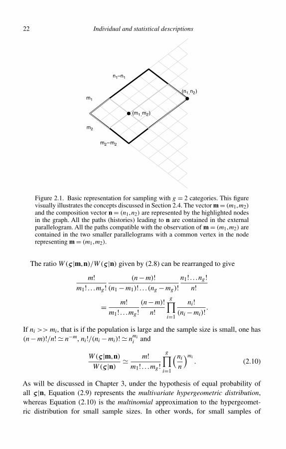
In Fig. 2.1, the case g = 2 is shown, for which a graphical representation is possible.The set of sequences producing n are delimited by thick lines, while those passingthrough m are delimited by two thin sets of lines.
22 Individual and statistical descriptions
n1–n1
m1
m2
m2–m2
(m1,m2)
(n1,n2)
Figure 2.1. Basic representation for sampling with g = 2 categories. This figurevisually illustrates the concepts discussed in Section 2.4. The vector m = (m1,m2)and the composition vector n = (n1,n2) are represented by the highlighted nodesin the graph. All the paths (histories) leading to n are contained in the externalparallelogram. All the paths compatible with the observation of m = (m1,m2) arecontained in the two smaller parallelograms with a common vertex in the noderepresenting m = (m1,m2).
The ratio W (ς |m,n)/W (ς |n) given by (2.8) can be rearranged to give
m!m1! . . .mg !
(n − m)!(n1 − m1)! . . . (ng − mg)!
n1! . . .ng !n!
= m!m1! . . .mg !
(n − m)!n!
g∏i=1
ni!(ni − mi)! .
If ni >> mi, that is if the population is large and the sample size is small, one has(n − m)!/n! n−m, ni!/(ni − mi)! nmi
i and
W (ς |m,n)
W (ς |n) m!
m1! . . .mg !g∏
i=1
(ni
n
)mi. (2.10)
As will be discussed in Chapter 3, under the hypothesis of equal probability ofall ς |n, Equation (2.9) represents the multivariate hypergeometric distribution,whereas Equation (2.10) is the multinomial approximation to the hypergeomet-ric distribution for small sample sizes. In other words, for small samples of
2.4 Partial and marginal descriptions 23
large populations, sampling without replacement and sampling with replacementvirtually coincide.
2.4.1 Example: Two agents selected out of n = 4 agents belongingto g = 3 categories
Consider n = 4 agents and g = 3 strategies (e.g. 1 = ‘bull’, optimistic; 2 = ‘bear’,pessimistic; 3 = ‘neutral’, normal), and assume that the joint α-description isω = (1,2,3,2). Now two agents are drawn without replacement (for a pizza witha friend):
1. List all sample descriptions (ςi)i=1,...,4.They are
{(1,2,2,3),(1,2,3,2),(1,3,2,2),(2,1,2,3),(2,1,3,2),
(2,2,1,3),(2,2,3,1),(2,3,1,2),(2,3,2,1),(3,1,2,2),
(3,2,1,2),(3,2,2,1)}.
Their number is W (ς |n) = 4!1!2!1! = 12.
2. Write all possible descriptions of the reduced sample (ςi)i=1,2.If the rule is applied and the first two digits of each permutation are taken, onegets some repetitions: {(1, 2), (1, 2), (1, 3), (2, 1), (2, 1), (2, 2), (2, 2), (2, 3),(2, 3), (3, 1), (3, 2), (3, 2)}, so that the possible descriptions are {(1, 2), (1, 3),(2, 1), (2, 2), (2, 3), (3, 1), (3, 2)}, and this is due to the fact that only ‘bears’ canappear together, as the draw is without replacement. It is useful to note that (1,2), (2, 1), (2, 2), (2, 3), (3, 2) can appear twice as the initial part of the completesequences, while (1, 3), (3, 1) can appear only once.
3. Write all possible frequency vectors for the reduced sample and count theirnumber.n = (1,2,1) as there are 1 bull, 2 bears and 1 neutral. The possible sampledescriptions are (1, 2), (1, 3), (2, 1), (2, 2), (2, 3), (3, 1) and (3, 2).Here (1, 2), (2, 1) belong to m = (1,1,0), and
W (ς |m,n) = m!m1! · · ·mg !
(n − m)!(n1 − m1)! · · ·(ng − mg)! = 2!
1!1!0!2!
1!1!1! = 4;
(2.11)
(1, 3), (3, 1) belong to m = (1,0,1), and W (ς |m,n) = 2!1!0!1!
2!0!2!0! = 2;
(2, 2) belongs to m = (0,2,0), and W (ς |m,n) = 2!0!2!0!
2!1!0!1! = 2;
24 Individual and statistical descriptions
(2, 3), (3, 2) belong to m = (0,1,1), and W (ς |m,n) = 2!0!1!1!
2!1!1!0! = 4. Note
that∑
m W (ς |m,n) =W (ς |n) = 12, where the sum is on the set {m :mi ≤ni,∑
mi = 2}.
2.5 Exercises
2.1 Prove that a set of n objects, divided into g classes with respect to the vari-ate X , with frequency vector (n1, . . . ,ng), can generate n!/(n1! . . .ng !) distincts-descriptions.
2.2 How many different samples can be drawn out of a population of n elements?2.3 Consider a system of five ‘energy elements’ (whose value is ε) allocated into
three molecules.1. Is it consistent to assume that the partition vector is (z0 = 1,z1 = 0,z2 =
1,z3 = 1)?2. What is its physical meaning?
2.4 Prove that the number of possible distinct occupation number vectors in asystem of n elements and g classes is
W (n|n,g) =(
n + g − 1
n
). (2.12)
2.5 Repeat the analysis of the Example in Section 2.4.1 for n = 3 and g = 3, thefollowing joint α-description, ω = (1,2,3) and a sample of 1 element.
2.6 Summary
In this chapter, the following descriptions were introduced for a set of n objects orelements partitioned into g classes with respect to a variate X.
The complete joint α-description gives the most complete characterization. Forinstance, for n = 4 and g = 3, the vector ω = (1,2,2,3) means that the first objectbelongs to class or category 1, the second and third objects to class or category 2and the fourth object to class or category 3.
By using the tool of sampling without replacement, one can pass from the jointα-description to the joint s-description. A joint s-description will be a permutationof the vector giving the joint α-description resulting from the process of samplingthe n objects without replacement. A possible joint s-description corresponding tothe joint α-description given above is ς = (2,1,2,3).
The occupation number vector gives the number of objects belonging to thevarious classes. For instance, in the case discussed above, one has n = (1,2,1)
meaning that there is one object belonging to class 1, two objects belonging toclass 2 and one object belonging to class 3.
2.6 Summary 25
The partition vector gives the number of classes with 0 up to n objects. In theexample, one has z = (0,2,1,0,0) and this means that there are zero classes with0 objects, two classes with 1 object, one class with 2 objects, zero classes with 3objects and zero classes with 4 objects.
Further reading
Boltzmann’s paper of 1868 is available in a collection of his works edited byF. Hasenöhrl.
L. Boltzmann, Studien über das Gleichgewicht der lebendigen Kraft zwischen bewegtenmateriellen Punkten, in WissenschaftlicheAbhandlungen, Volume 1, edited by F. Hasenöhrl,Barth, Leipzig (1868).
A contemporary account of Boltzmann’s method can be found in a paper by Bach.
A. Bach, Boltzmann’s probability distribution of 1877,Archive for History of Exact Science,41, 1–40 (1990).
Bach also discusses the basic descriptions on which this chapter is based. Thereader can also refer to Ya.G. Sinai’s book for a simple approach to the descriptionof finite sets.
Ya.G. Sinai, Probability Theory. An Introductory Course, Springer-Verlag, Berlin, Heidel-berg (1992).
For basic statistical notions one can see Kendall and Stuart’s book.
M.G. Kendall and A. Stuart, The Advanced Theory of Statistics, 2nd edition, Volume 1,Griffin & Co., London (1953).
Much of this chapter is based on elementary combinatorics. Merris’ textbook con-tains a clear statement of the fundamental counting principle. The first two chaptersof his book contain most of the proofs and material needed to read this chapterwith profit.
R. Merris, Combinatorics, Wiley, Hoboken, NJ (2003).
A standard reference for combinatorics, available in virtually all maths libraries,is the first volume of Feller’s monograph on probability. Probably influenced byquantum mechanical problems, Feller uses the concepts of distinguishable andindistinguishable objects, which to the authors of this book appear redundant andperhaps misleading.
W. Feller, An Introduction to Probability Theory and its Applications, 2nd edition, Volume 1,Wiley, New York (1957).
In Chapter 7, quantum statistics is derived in the framework of a classical modeldeveloped by Brillouin and without using indistinguishability.
3
Probability and events
In this chapter, the space of all individual descriptions compatible with what isknown on a finite population is introduced. This is an instance of what probabilistscall either sample space or set of logical possibilities or set of elementary descrip-tions; it is usually represented by the symbol �. The subsets of � can be composedby means of logical connectives, and the resulting algebra is an algebra of subsetsof the sample space. Each element of this algebra is called an event. Each eventcan be assigned a non-negative real number in the interval [0,1]: its probability.Given a set of mutually disjoint and exhaustive events, their probabilities sum upto 1. Individual decompositions will be defined, whose meaning is the probabilitydistribution for the ith agent to be in each category.
If you already know elementary probability theory, you can read the chapterdirectly and skip the appendix. For those who are not familiar with elementaryprobability theory, an appendix explains the basic concepts needed to read thechapter with profit.
After studying this chapter, you should be able to:
• understand the notion of an event, as a collection of joint descriptions;• understand the composition of two events in terms of union and intersection, and
the complement of an event;• define the notion of probability space;• discuss some deep hypotheses usually added to the basic axioms of probability;• use simple urn models, in order to compute predictive probabilities.
3.1 Elementary descriptions and events
As discussed in Chapter 2, a system of n elements classified into g categories canbe described by some alphabetic list ω = (ωi)i=1,...,n or any equivalent sampledescription, or by the occupation-number vector n = (nj)j=1,...,g , or by frequencyvectors of occupation numbers a.k.a. partition vectors: z = (zk)k=0,...,n. The most
26
3.1 Elementary descriptions and events 27
fundamental descriptions of the system are the individual sequences ω; setting upa probability space for these descriptions is equivalent to considering the space �
including all possible individual sequences. Here, it is not necessary to distinguishbetween α- and s-descriptions. An element (an outcome, a point) of � is denotedby ω = (ω1, . . . ,ωn), with ωi ∈ X = {1, . . . ,g}, and its cardinality is #� = gn. Anevent is a subset of �.
As � is a finite set with gn elements, the family P(�) of all subsets of � (itspower set), including � itself and the empty set ∅, is finite, as well, and it has 2gn
elements. In this finite case we can state that every set A belonging to P(�), insymbols A ∈ P(�), is an event. P(�) is closed under the binary operations of union∪ and intersection ∩ and the unary operation of complementation. In other words,if A ∈ P(�) and B ∈ P(�), then A ∪ B ∈ P(�), A ∩ B ∈ P(�) and Ac ∈ P(�).
3.1.1 Example: dichotomous wealth distribution
In order to illustrate the above considerations with an example, consider a system ofthree agents, Alice, u1, Bob, u2, and Charles, u3, and two qualities, poor (not rich),P = 1, and rich, R = 2. The fundamental description of this system is assumed tobe one of the 23 = 8 individual sequences ω = (ω1,ω2,ω3) with ωi ∈ {1,2}. Beforeobserving the system, what can one expect regarding the wealth distribution of thissmall population?
The set of all individual descriptions is � = {ωi, i = 1, . . . ,8}, in detail ω1 =(1,1,1), ω2 = (1,1,2), ω3 = (1,2,1) , ω4 = (1,2,2), ω5 = (2,1,1), ω6 = (2,1,2),ω7 = (2,2,1), ω8 = (2,2,2).
All subsets of � are events. The simplest events in � are the singletons, suchas {ω5}, containing a single joint description. Observe that the vector ω5 describesa world where Alice is rich while Bob and Charles are poor, whereas the set {ω5}is an event true if ω5 occurs. One should consider descriptions as facts (takingplace or not), and events as propositions (true or not) about facts (taking placeor not). This useful distinction is borrowed from Wittgenstein’s Tractatus Logico-Philosophicus [1].
The event {ω1,ω2} is true when both Alice and Bob are poor, irrespective ofCharles’ wealth. Note that {ω1,ω2} = {ω1}∪ {ω2}.
Some events are worthy of special attention. Let A(i)j denote the event in which
the ith individual is in state j: ωi = j (see Section 2.4). For instance A(2)1 denotes the
event A(2)1 = {ω1,ω2,ω5,ω6}; A(2)
1 is true when Bob is rich, irrespective of Alice’sand Charles’ status. A singleton, {ωi}, can be written as the intersection of threemarginal events. As an example, one has {ω8} = A(1)
2 ∩A(2)2 ∩A(3)
2 ; this event is trueif Alice, Bob and Charles are rich.
28 Probability and events
Moreover, the complement (negation) of an event is still an event: {ω8}c ={ω1,ω2, . . . ,ω7} is the event that is true if at least one agent is poor. It can bedirectly checked that every set operation ∪, ∩ and c on subsets of � yields someset in P(�), including � and the empty set ∅.
Suppose one is interested in checking whether Alice is rich. The event A(1)1 = A1
(for ease of notation) is true if Alice is rich. In order to plan an empirical obser-vation, one must consider all the possibilities, and in order to complete a Booleanlattice (see Section 3.6), one has to introduce at the least the complement Ac
1 = A2
as well, the event true if Alice is not rich. If the options were g instead of 2,here one would further consider all the marginal events Aj, j = 2, . . . ,g. Startingfrom A1 and A2 and combining them by intersection, union and complementation,one finds only two new events, namely � = A1 ∪ A2, whose meaning is ‘Aliceis rich or not rich’ – a truism – and ∅=A1 ∩ A2, whose meaning is ‘Alice isboth rich and not rich’ – a contradiction. Hence, the lattice (algebra) generatedby A1 is σ(A1) = {∅,A1,A2,�}, and {A1,A2} are the constituents (a.k.a. atoms) ofthe lattice.
If Bob is taken into account as well, starting from the two events A1 (‘Alice isrich’) and A(2)
1 = B1 (‘Bob is rich’) whose complement is B2 and considering allthe intersections Cij = Ai ∩ Bj; i, j = 1,2, any event concerning the wealth of Aliceand Bob is obtained as a union of the sets Cij.
The simplest probability assignment for the system discussed above is the uni-form distribution on all the individual descriptions. If one introduces a non-negativeweight function such as p(ω1) = . . . = p(ω8) and
∑8i=1 p(ωi) = 1, then, for any
i, p(ωi) = 1/8. In this case, given that P(C) =∑ω∈C p(ω), it turns out that theprobability of any event is proportional to the number of individual descriptions itcontains. In other words, one gets
P(C) = #C
#�; (3.1)
this is nothing else but the number of favourable cases divided by the number ofpossible cases, coinciding with the so-called classical definition of probability givenby Equation (1.1). Each agent has four possibilities for being rich, then P(A(i)
1 ) =4/8 = 1/2, for i = 1,2,3. The same applies to being poor, as A(i)
2 = A(i)c1 , and as
a consequence of the axioms of probability, one has that P(A(i)c1 ) = 1 − P(A(i)
1 ) =1/2. Note that for any singleton P({ω}) = P(A(1)
ω1 ∩ A(2)ω2 ∩ A(3)
ω3 ) = 1/8 and thatP(A(1)
ω1 )P(A(2)ω2 )P(A(3)
ω3 ) = 1/23 = 1/8. Hence
P
(A(1)
ω1∩ A(2)
ω2∩ A(3)
ω3
)= P
(A(1)
ω1
)P
(A(2)
ω2
)P
(A(3)
ω3
). (3.2)
3.2 Decompositions of the sample space 29
This means that the n sub-experiments A(i) = {A(i)1 , . . . ,A(i)
g } , each of them describ-ing the observation of the ith individual, are independent. In other words, animportant consequence of assigning the uniform distribution on the set of individualdescriptions is the independence of the marginal events. Moreover, P(A(i)
ωi ) = 1/2does not depend on i, the label of the agent, and agents are equidistributed, inother words the probability of belonging to a category is the same for all the gagents. Finally, it does not depend on ωi, meaning that the distribution is uniformfor each agent.
3.2 Decompositions of the sample space
As discussed in the appendix, a decomposition of the sample space � is a familyof events E = {Ei : Ei ∩ Ej = ∅, ∪n
i=1Ei = �}. Note that, for ease of notation andfollowing common usage, from now on, the intersection symbol ∩ between sets issometimes omitted when no confusion is possible.
Given a decomposition E = E1, . . . ,En of �, the probabilities P(Ei) are theprobability distribution associated with E and
∑ni=1 P(Ei) = 1.
The collection of all singletons is the thinnest decomposition of the descriptionspace �, or � = Eω = {{ω} : ω ∈ �}; the singletons are mutually disjoint and theirunion is �. For the sample space of individual descriptions #Eω = gn. However,this is not the only possible decomposition of �. Note that both {n} and {z} areevents (subsets of �); they were discussed in Chapter 1 and, given their properties,it is possible to verify that
• the set of distinct occupation vectors En = {n = (n1, . . . ,ng) :∑g
1 nj = n} is a
decomposition of �, with #En =(
n + g − 1
n
);
• the same holds true for the set of the distinct partition vectors Ez ={z = (z0 . . .zn) :∑n0 zi = g,
∑n0 izi = n};
• it follows that∑
n∈EnP(n) =∑z∈Ez
P(z) = 1.
All the above decompositions are associated with experiments involving allindividuals and categories.
• If the attention is fixed on the ith sub-experiment, {A(i)1 , . . . ,A(i)
g } is a decomposi-tion of � and its meaning is that the ith observed agent will result in one and onlyone value of {1, . . . ,g}. Therefore (P(A(i)
j ))j=1,...,g is the probability distribution
associated with the ith observed agent, and∑g
j=1 P(A(i)j ) = 1.
• If the attention is fixed on a specific category j, and all individuals are classifiedas belonging or not to this category, one has a dichotomous partition of � of thekind n = (nj,n − nj) (see Section 2.4).
30 Probability and events
3.2.1 Example: the symmetric binomial distribution
Considering the example of Section 3.1.1, one can group the individual descriptionsaccording to their occupation number vectors n1 = # poor, n2 = # rich. In thisexample, each vector n = (n1,n2) represents a wealth distribution, whereas in theExample of Section 2.3.2, the wealth distribution was described by a partition vectorz. Indeed, here, the objects to be allocated into categories are agents, and in Section2.3.2 the objects were coins, to be distributed into categories there representedby agents. Also, here, the total wealth is not fixed, but in Section 2.3.2 it wasfixed. The possible occupation vectors as well as the corresponding individualdescriptions are listed below. ω1 = (1,1,1) corresponds to (n1 = 3,n2 = 0): Alice,Bob and Charles are all poor. (n1 = 2,n2 = 1) contains three descriptions, ω2 =(1,1,2), ω3 = (1,2,1), ω5 = (2,1,1); these are the cases with two poor agentsand a rich one. (n1 = 1,n2 = 2) contains three descriptions too, ω4 = (1,2,2),ω6 = (2,1,2), ω7 = (2,2,1); these are the cases with a rich agent and two poorones. Finally, ω8 = (2,2,2) is the happy situation where all the agents are rich,(n1 = 0,n2 = 3).
All the possible occupation number vectors are a decomposition of �. If theindividual joint descriptions are equiprobable, one gets P(n1 = 3,n2 = 0) = P(n1 =0,n2 = 3) = 1/8, and P(n1 = 2,n2 = 1) = P(n1 = 1,n2 = 2) = 3/8. Given theconstraint n2 = 3−n1, the probability distribution on the statistical description canbe written as
P(n1 = k) =(
3
k
)(1
2
)3
, k = 0, . . . ,3. (3.3)
Therefore, the probability of the occupation n can be written as the probability ofa given sequence (1/2)3 multiplied by the number of sequences W (ς |n) given byEquation (2.3). For n agents then
P(n1 = k) =(
n
k
)(1
2
)n
, k = 0, . . . ,n, (3.4)
that is the symmetric binomial distribution.As for the partition vectors, (n1 = 3,n2 = 0) and (n1 = 0,n2 = 3) belong to
(z0 = 1,z1 = 0,z2 = 0,z3 = 1), meaning that one category is empty and the othercontains all the three agents; (n1 = 2,n2 = 1) and (n1 = 1,n2 = 2) belong to (z0 =0,z1 = 1,z2 = 1,z3 = 0). Note that the constraints allow only two values of z. FinallyP(z0 = 1,z1 = 0,z2 = 0,z3 = 1)=P(n1 = 0,n2 = 3)+P(n1 = 3,n2 = 0)= 2/8 = 1/4and P(z0 = 0,z1 = 1,z2 = 1,z3 = 0) = P(n1 = 1,n2 = 2)+P(n1 = 2,n2 = 1) = 3/4.
3.2 Decompositions of the sample space 31
One could bet 3 : 1 to find elements divided into two clusters, and 1 : 3 to find themall in the same state of wealth.
3.2.2 Example: the Ehrenfest urn
Let us consider a box, divided into two symmetric communicating parts, and nmolecules free to move from one part to the other. If all the individual descriptionsof n molecules on g = 2 states are equiprobable then each molecule has probability1/2 to be found either on the left or on the right part of the box, and this probabilityis independent from the state of other molecules. Considering the description n =(n1,n2 = n − n1), due to the constraint n1 + n2 = n, as above one has
P(n1 = k) =(
n
k
)(1
2
)n
, k = 0,1, . . . ,n. (3.5)
Note that due to symmetry P(n1 = k) = P(n1 = n− k) = P(n2 = k), and given thatthe symmetric binomial distribution is bell-shaped the most probable occupationvector is close to k = n/2. Conversely the probability of finding all molecules on thesame side is 2(1/2)n. The tendency to a fifty–fifty allocation of molecules increasesvery rapidly as a function of the number n of molecules. This looks quite reasonablein the case of gas diffusion.
3.2.3 Example: energy distribution of two molecules
Coming back to Boltzmann’s ideas (see the Example in Section 2.3.1), let us assumethat all the individual descriptions of n energy elements ε = E/n on g = 2 moleculesare equiprobable: each element has probability 1/2 of belonging to one moleculeor to the other; this probability does not depend on the behaviour of any otherenergy element. By using the previous examples, one can see that the probabilitythat the first molecule has energy equal to E1 = kε, or, equivalently, that it containsa fraction of the total energy k(E/n), is
P(E1 = kε) =(
n
k
)(1
2
)n
, k = 0,1, . . . ,n. (3.6)
If n is even, the most probable value is n/2, that is E1 = E/2. In the case ofg molecules, the most probable value for any molecule would have been E/g.This looks reasonable, but a bit of inspection is enough to show that this cannotbe the case. Boltzmann observed that in the continuous limit ε → 0, and n →∞ with E = nε, each molecule would have energy E/g with probability one,in disagreement with Maxwell’s energy distribution. This means that a uniformdistribution of energy elements on molecules cannot be the right one.
32 Probability and events
3.3 Remarks on distributions
The uniform distribution is often presented as a ‘milestone’ of probability theory.As already discussed in the introductory chapter, this is due to historical reasons,and to the widespread application of this approach to gambling. Methods due toLaplace were discussed, criticized and finally abandoned during the nineteenthcentury, when probability started to be applied to the social sciences, to physics,to statistics as well as to genetics. The difficulty related to equiprobable ‘possiblecases’ from which ‘favourable ones’ are taken based on counting can be tracedback to J. Bernoulli’s Ars Conjectandi and to Bernoulli’s theorem (see referencesof Chapter 1). The problem of the so-called ‘inversion’ of Bernoulli’s theorem(that is estimating probabilities via observed frequencies) is the core subject ofBayes’ memoir Essay Towards Solving a Problem in the Doctrine of Chancespublished posthumously in 1763 in the Philosophical Transactions of the RoyalSociety (see references of Chapter 1). As a matter of fact, for any probability spacethere are as many possible uniform probability distributions as decompositionsof the sample space. If you wish to follow the ‘indifference principle’ and thenuse a uniform distribution somewhere, which decomposition of the sample spaceshould you prefer?
3.3.1 Independence and identical distribution of events:the multinomial distribution
From the uniform distribution on all individual descriptions1
P({ω}) = 1
#�= 1
gn, (3.7)
one derives that the individual events A(i)ωi are independent, have the same probability
distribution and this distribution is uniform. Note that (3.7) does not contain anyparameter added to n and g. Considering that any function P(·) satisfying theaxioms of probability is worthy of study, it is now time to move from (3.7) to a P(·)containing a parameter vector (pi ≥ 0)i=1,...g ,
∑gj=1 pj = 1 by setting
1. P({ω}) = P(A(1)ω1 . . .A(n)
ωn ) = P(A(1)ω1 ) . . .P(A(n)
ωn ),2. P(A(i)
ωi ) = pj if ωi = j. In this case P({ω}) =∏gj=1 p
njj ,
where nj is the number of ωi = j, that is the number of agents in the jth category.
The meaning is as follows: the notation A(i)j denotes all the joint descriptions for
which ωi = j, that is the ith element of the description belongs to the jth category;
1 In the following, when no confusion is possible, both {ω} and ω will be called individual descriptions.
3.3 Remarks on distributions 33
this notation was introduced in Section 3.1.1; therefore P(A(i)ωi ) is the probability
that the ith element belongs to the category denoted by ωi; for instance, P(A(2)1 ) is
the probability that the second element is in the first category. If P(A(i)j ) = pj, then
the probability of belonging to the jth category coincides for all the elements. IfP({ω}) =∏g
j=1 pnjj holds, the events {A(i)
ωi }i=1,...,n are still independent and identi-cally distributed (i.i.d.), but this distribution is no longer uniform, except in thecase pj = 1/g, bringing us back to the uniform distribution on the joint indi-vidual descriptions. At odds with (3.7), all individual descriptions are no longerequiprobable, as their probabilities depend on the occupation vector n. However,it is still true that all the descriptions belonging to the same occupation vectorn have the same probability. The probability of an occupation vector n is theprobability of a given individual description multiplied by the number of possiblesequences belonging to the same occupation vector n, which is given by Equation(2.3). In other words, one gets the multinomial distribution of parameters n andp = (p1, . . . ,pg):
P(n) = MD(n;p) = n!n1! · · ·ng !
g∏j=1
pnjj , (3.8)
where MD(n;p) is a shortcut for denoting the last term in Equation (3.8).
3.3.2 Example: casting a die with skewed prize
If a fair die gives ‘1’ the prize is 0, if it gives ‘2 or 3’ the prize is 1, if it gives‘4 or 5 or 6’ the prize is 2. What is the probability of a prize 0 after throwing thedie three times? In order to solve this problem, consider the �-space of a fair diecast three times using these descriptions ω = (ω1,ω2,ω3), ωi ∈ {1,2,3,4,5,6}, andintroducing the individual events A(i)
ωi which occur if the ith throw gives ωi. Theprize associated with the ith throw is the event G(i)
ξi, ξi ∈ {0,1,2}, and G(i)
0 = A(i)1 ,
G(i)1 = A(i)
2 ∪ A(i)3 , G(i)
2 = A(i)4 ∪ A(i)
5 ∪ A(i)6 . If all the descriptions in � have the
same probability, one can set pi = P(G(i)ξi
) and obtain p0 = 1/6, p1 = 2/6 = 1/3,
p2 = 3/6 = 1/2, with∑2
i=0 pi = 1 as for any throw (G(i)ξi
)ξi∈{0,1,2} is a partition ofthe sample space. One gets the prize 0 if and only if ω = (1,1,1), and P(1,1,1) =P(A(1)
1 )P(A(2)1 )P(A(3)
1 ) = p30 = (1/6)3 = 1/216.
Alternatively, one can use the new sample space �(ξ) composed of all the descrip-tions ξ = (ξ1,ξ2,ξ3), with ξi ∈ {0,1,2} which directly give the prize associated witheach throw. Note that �(ξ) only has 33 elements, whereas the previous samplespace contained 63 elements. A probability assignment on �(ξ) consistent with theprevious one is pξ = pξ1pξ2pξ3 , where pξi = 1/6 if ξi = 0, pξi = 1/3 if ξi = 1 and
34 Probability and events
pξi = 1/2 if ξi = 2. In this way
P({ξ}) =2∏
i=0
pnii , (3.9)
where ni is the number of ξj = i, that is the number of throws with the ith prize.Again, one gets P(0,0,0) = (1/6)3 = 1/216.
As mentioned at the end of Section 3.3.1, the probability of getting n0 times theprize 0, n1 times the prize 1 and n2 times the prize 2 is
P(n) = 3!n0!n1!n2!
2∏i=0
pnii . (3.10)
This is an instance of the multinomial distribution MD(n;p) with n = 3, p =(1/6,1/3,1/2).
This example shows that the events needed to represent the problem can bebuilt out of any suitable sample space �. Moreover, recalling the example inSection 3.1.1, one is not obliged to represent a lattice (algebra) by means of all itssets. What is essential is that probability values are assigned to all the atoms (con-stituents) of the lattice. In the present case, this means fixing P(G(1)
ξ1∩G(2)
ξ2∩G(3)
ξ3)
for any value ξ1,ξ2,ξ3 representing the thinnest decomposition of � relevant forthe problem. Instead of 3 · 3 − 1 = 8 free probability values, the assumed indepen-dence and equidistribution of events belonging to different trials reduces the freeprobability values to 3 − 1 = 2.
3.3.3 Sampling without replacement: the multivariatehypergeometric distribution
As in Section 2.1.3, suppose one knows that the set of five firms is described byω = (1,1,2,3,2). If a random sample of size 2 is drawn, what is the probability ofobtaining two firms belonging to the sector labelled by 1? In order to answer thisquestion, one first notices that a complete random sampling without replacement isa sequence (ς1,ς2,ς3,ς4,ς5) given by a permutation of (1,1,2,3,2). The number ofdistinct permutations can be obtained from Equation (2.3) with n = 5, n1 = n2 = 2and n3 = 1:
n!n1!n2!n3! = 5!
2!2!1! = 30. (3.11)
The conditioned sample space can be denoted by the symbol
�(ς)n = {(ς1,ς2,ς3,ς4,ς5)|n = (2,2,1)}. (3.12)
3.4 Probability assignments 35
It is usual to assume that all the possible samples ς have the same probability; inthe present case this assumption leads to:
P(ς |n) =(
n!n1!n2!n3!
)−1
= 1
30. (3.13)
Indeed, the assumption
P(ς |n) =(
n!n1! . . .ng !
)−1
, (3.14)
can be regarded as a definition of random sampling, and can be justified both froman objective and from a subjective point of view. With this assumption, it is possibleto relate all the combinatorial formulae in Section 2.4 to probabilities. In particular,Equation (2.9) becomes
P(m) = HD(m;n) =∏g
i=1
(ni
mi
)(
n
m
) , (3.15)
which is the multivariate hypergeometric distribution of parameters n, n.In the example discussed above, there are g = 3 categories, and one has n = 5,
n = (2,2,1) and m = 2, m = (2,0,0). Therefore, by means of the hypergeometricdistribution, one gets
P(m = (2,0,0)) =
(2
2
)(2
0
)(1
0
)(
5
2
) = 2!3!5! = 2
5 · 4= 1
10. (3.16)
Note that the set of distinct m = (m1,m2,m3), such that m1 + m2 + m3 = 2, has6 elements in agreement with Equation (2.5).
3.4 Probability assignments
Contrary to other approaches, Kolmogorov’s axiomatic method does not provideany tool to determine event probabilities. Therefore, in order to assign probabilities,it is necessary to use other considerations and, as discussed in Chapter 1, the indif-ference principle is often useful. In this section, probability assignments to samplespaces related to the partition of n objects into g categories will be further discussed.The classical definition (3.1), when applied to the sample space of n elements and gcategories, leads to Equation (3.7), meaning that all the individual descriptions
36 Probability and events
are equiprobable, and the events A(1)ω1 , . . . ,A(n)
ωn are independent, identically anduniformly distributed. In particular, one has P(A(i)
j ) = 1/g.
When applied to the conditional sample space �(ς)n , the same assumption (3.1)
assigns equal probability to all the descriptions belonging to n. Now, the situa-tion is quite different: the events {A(i)
ωi }i=1,...,n are still identically distributed, withprobability P(A(i)
j ) = nj/n for all individuals, but they are no more independent.
3.4.1 Absolute and predictive probability assignments
There are two possible ways of assigning probabilities to events in the samplespace �. As mentioned before, the thinnest partition of � is given by the eventscorresponding to the individual descriptions ω. On this partition, a probabilityfunction is obtained defining a function p(ω) ≥ 0 for each description ω, with thecondition
∑ω p(ω) = 1. The singletons {ω} can be written as the intersection of n
marginal events, leading to
p(ω) = P({ω}) = P
(A(1)
ω1. . .A(n)
ωn
). (3.17)
The absolute method consists in fixing the left-hand side of (3.17) and derivingP(E) for any event E by adding the probabilities of all the individual descriptionswhose union gives E.
The alternative predictive method is based on the calculation of the right-handside of (3.17) using the multiplicative rule based on conditional probabilities:
P
(A(1)
ω1. . .A(n)
ωn
)= P
(A(1)
ω1
)P
(A(2)
ω2|A(1)
ω1
). . .P
(A(n)
ωn|A(1)
ω1. . .A(n−1)
ωn−1
). (3.18)
The probability assignment to the sequence is built step-by-step by giving proba-bility values to the next subresult, conditioned on the previous subresults. In manyinteresting cases, predictive probabilities can be interpreted in terms of urn models.The knowledge of P(A(m+1)
j |A(1)ω1 . . .A(m)
ωm ) for any m = 0,1, . . . ,n−1 is equivalent tothe knowledge of the probability of the singletons {ω} from which the probabilityof A(i)
j can then be recovered using the absolute method (see Exercise 3.4). Thepredictive method is very intuitive, and it is valid also in the case n → ∞, typi-cal of stochastic processes (see Chapter 4). The quantities P(A(m+1)
j |A(1)ω1 . . .A(m)
ωm )
are called predictive probabilities. In the independent and identically distributedcase they are
P
(A(m+1)
j |A(1)ω1
. . .A(m)ωm
)= pj, (3.19)
3.4 Probability assignments 37
where, indeed, the probability of being in the jth class does not depend on the indexof the individual (identical distribution) and does not depend on the allocation ofprevious observed individuals as well (independence).
In the case of equiprobability of all descriptions belonging to n, the predictiveprobabilities are:
P
(A(m+1)
j |A(1)ω1
. . .A(m)ωm
)= nj − mj
n − m, (3.20)
where mj ≤ nj is the number of observations belonging to the jth category up tostep m. The meaning of this formula can be clarified by the usual model for such asituation: an urn of known composition n = (n1, . . . ,ng), with
∑gi=1 ni = n, where
the g categories represent g colours. Balls are drawn without replacement from theurn. If at each draw all the balls remaining in the urn have the same probabilityof being drawn, one gets P(A(1)
j ) = nj/n, P(A(2)j |A(1)
i ) = (nj − δj,i)/(n − 1), . . .,and, in general, all the equations summarized by (3.20) have an interpretation interms of event probabilities within the urn model. In this case events are negativelycorrelated, as drawn balls of given colours reduce the probabilities of drawing thesame colours (see Exercise 3.4). As a final remark, in Chapters 4 and 5, it will beshown that (3.19) leads to the multinomial distribution (3.8) whereas (3.20) leadsto the multivariate hypergeometric distribution (3.15).
3.4.2 Degrees of freedom for a probability assignment
In general, in order to define a probability function on the sample space of n elementsand g categories we need to fix gn −1 probability values. The uniform distributionassignment is the simplest, as everything follows from the knowledge of only twoparameters: g and n. The independent and identically distributed case is slightlymore complicated, as it requires a set of g−1 parameters pj ≥ 0, such that
∑gj=1 pj =
1, representing the marginal probability that an object belongs to the jth class. Thecase of a sample space conditioned on a given occupation number also has g − 1degrees of freedom, as it requires a set of g − 1 parameters nj ≥ 0, such that∑g
j=1 nj = n, representing the distribution of the n objects into the g classes.As discussed above, the case of the n-conditional sample space has an interpre-
tation in terms of an urn model. Indeed, the independent case also can be describedin terms of an urn model: an urn where balls of g different colours are drawn withreplacement and where pj is the probability of drawing a ball of the jth colour.Recall that in the other case the parameter nj represents the initial number of ballsof colour j.
There is a more difficult case when one considers that all occupation vectors arepossible, and P(n) is the probability distribution on them. In this case, the number
38 Probability and events
of degrees of freedom df is
df =(
n + g − 1
n
)− 1. (3.21)
If also in this case it is assumed that, conditional on n, all the compatible descrip-tions are equiprobable, according to Equation (3.14), this probability space can beinterpreted in terms of draws from an urn with uncertain composition, and P(n)
describes this uncertainty.
3.4.3 Example: again on molecules and energy elements
Coming back to the example of Section 3.2.2, assume now that all occupation vec-tors of n energy elements on g = 2 molecules are equiprobable; this means that all thedescriptions (n,0), (n−1,1), . . ., (1,n−1), (0,n) have the same probability. Whenthe continuous limit is taken, this hypothesis leads to the fundamental hypothesisof classical statistical mechanics, that is equal a-priori probability of all moleculardescriptions compatible with the total energy. Given that Equation (3.14) holds,a joint description ω of the n elements has a probability depending on (k,n − k).One finds
P({ω}) =∑
k
P({ω}|k)P(k) = P({ω}|k)P(k), (3.22)
given that there is only a value of k compatible with ω. Moreover, P(k) is uniform,that is P(k) = 1/(n + 1), and as a consequence of (3.14):
P({ω}|k) =(
n!k!(n − k)!
)−1
, (3.23)
leading to, as a consequence of (3.22):
P({ω}) = 1
n + 1
k!(n − k)!n! . (3.24)
Thus, the assumption of uniform probability on occupation vectors leads to a non-uniform distribution for the individual descriptions where the probability of eachindividual description only depends on k, the number of energy elements belongingto the first molecule. This probability is maximum for k = 0 and k = n, correspond-ing to the occupation vectors (0,n), and (n,0), where it reaches the value 1/(n+1),whereas, for even n, the minimum is in (n/2,n/2). In other words, there are manydescriptions corresponding to the vector (n/2,n/2), and the sum of their weights
3.5 Remarks on urn models and predictive probabilities 39
coincides with the weight of ω = (1, . . . ,1), the only description correspondingto (n,0). It can be shown that the predictive probability ruling such individualdescriptions is
P
(A(m+1)
j |A(1)ω1
. . .A(m)ωm
)= 1 + mj
2 + m. (3.25)
Indeed, applying Equation (3.25) to the fundamental sequence made up of k valuesequal to 1 followed by n−k values equal to 2 leads to the following value of P({ω}):
1
2
1 + 1
2 + 1· · · 1 + k − 1
2 + k − 1
1
2 + k
1 + 1
2 + k + 1· · · 1 + n − k − 1
2 + n − 1= 1
n + 1
k!(n − k)!n! , (3.26)
corresponding to the value obtained above. This value does not depend on theorder in which the k components equal to 1 appear in the sequence. As will be clearin Chapter 7, Equation (3.25) can be used to derive the so-called Bose–Einsteinstatistics using a purely probabilistic approach due to Brillouin. For this reason,some scholars claimed that the Bose–Einstein statistics was originally discoveredby Boltzmann while trying to derive Maxwell’s distribution of velocities in a gas.Note that the Boltzmann method considered n energy elements into 2 molecules,whereas the derivation of Bose–Einstein statistics would be based on n moleculesinto 2 states.
The probability of allocating the first energy element to the first molecule is1/2, but the probability of the mth element being assigned to the first moleculedepends on the allocation of all the previous energy elements. Contrary to (3.20),this probability is an increasing function of the number of ‘successes’in the previoustrials. This process can be described by means of an urn model as well: the so-calledPólya urn. Consider an urn containing balls belonging to two categories, the firstcategory of balls is labelled with 1 and the second one is labelled with 2. At thebeginning, half of the balls are of type 1 and the other half are of type 2. Each timea ball is drawn, it is replaced into the urn, together with a new ball of the same type.If, at any draw, all the balls in the urn have the same probability to be selected,Equation (3.25) follows.
3.5 Remarks on urn models and predictive probabilities
3.5.1 Urn models, accommodation models and possible misunderstandings
Urn models are commonly used, but, often, their probabilistic meaning is unclear.In the case of equiprobability of all the individual descriptions corresponding to theoccupation vector n, the predictive probability is given by the ratio of nj −mj overn−m, where nj is the number of individuals or objects belonging to category j, mj
is the number of observed individuals belonging to j and nj − mj is the number of
40 Probability and events
individuals belonging to the jth category not yet observed; moreover, n denotes thetotal number of individuals and m is the number of observations, so that n−m is thetotal number of individuals yet to be observed. Here, there is a perfect isomorphismbetween observing individuals from a given population and drawing balls froman auxiliary urn, whose initial composition is n1, . . . ,ng and corresponds to thecomposition of the population. Indeed, even today, statisticians can use balls in one-to-one correspondence with real objects in order to randomly sample individualsfrom a finite population. In this case, one can imagine that the sample is createdstep by step, and when one has a sample described by m, a description of thesampled population is given by the vector (m1, . . . ,mg), with mi ≤ ni. When mequals n, sampling must stop and the auxiliary urn is empty. Now, all the populationhas been transferred to the sample, or better the sample coincides with the wholepopulation.
Starting from this pertinent example, it is tempting to extend urn models toindependent predictive probabilities. In such a case, one has predictive probabilitiesgiven by (3.19) with pj ∈ Q, rational number, and the auxiliary urn contains nj = Npj
balls of type j, where N : Npj ∈ N for all js and the drawn ball is replaced in orderto preserve independence and equidistribution for all draws. In this case, there isno real correspondence between balls and individuals, the fractions of balls of typej in the urn are a mere expedient to produce the correct sequences of drawn values.This mechanism is valid for any sample size 0 < m ≤ n, and it could be extendedto any number of trials.
Returning to the example of n energy elements to be allocated into g molecules,one can imagine having a system of g colours. The predictive probability (here withthe meaning of an allocation probability)
P
(A(m+1)
j |A(1)ω1
. . .A(m)ωm
)= 1 + mj
g + m, (3.27)
can be represented by a Pólya urn model, whose initial content is g balls, one foreach colour; then the urn is updated after each draw by replacing the drawn balland by adding a ball whose colour is the same. Again, the Pólya urn model isnothing else than an expedient tool to assign probability values. At the end of theaccommodation process, one still has n energy elements in the system, but n + gballs in the Pólya urn.
While in the hypergeometric case, the urn and the population to be examinedhave the same cardinality, so that the drawing process necessarily ends after n steps,in the Bernoullian case, when the population to be examined decreases to zero, thecomposition of the auxiliary urn stays constant, and in the Pólya case the contentof the urn increases.
3.5 Remarks on urn models and predictive probabilities 41
3.5.2 A realistic interpretation of the predictive probability
So far, two kinds of individual description have been discussed: alphabeticaldescriptions and sampling descriptions. This difference refers to the meaning of theindex i in the event A(i)
ωi , that is the object which is examined in the ith observation.Assume that the Body-Mass-Index (BMI) of a population of size n is studied; onecould believe that the allocation of n individuals into g BMI classes is a datumthat observation simply discovers. In this sense an alphabetical description of indi-viduals into g BMI classes admits a probabilistic description only if one considersprobability as a measure of ignorance; even if each individual is indeed allocated tosome BMI class, it is not known to which class the individual belongs. Even if the(frequency) vector of the population is known, an orthodox (frequentist) statisticianwould say that there is a single alphabetical description that is true but unknown, sothat the set of possible individual descriptions cannot be a domain for probability.
It is a quite different situation if, given the frequency vector n, one draws allindividuals without replacement at random. Indeed, it is important to stress thatthe deep meaning of the term at random is far from clear, and it resisted researchwork by scholars such as von Mises, Church, Kolmogorov and so on. Insteadof at random it is advisable to use the cautious expression all elements beingequiprobable with respect to drawing. As mentioned above, the equiprobability ofall sequences P({ς}|n) = (W (ς |n))−1, that is Equation (3.14), is widely acceptedas the most important axiom in mathematical statistics.
The above discussion concerns the common statistical context where the alloca-tion of objects into categories is a datum preceding the statistical analysis. However,this is not the case that will be discussed in the following. First of all, one wouldlike to describe individuals (or agents) changing category as time goes by; there-fore, alphabetical descriptions will change in time as well. Incidentally, in thisframework, the probability P({ω}) has a natural frequency interpretation in termsof the time fraction in which the description ω is true. Secondly, as mentioned atthe beginning of Section 3.5.1, the predictive probability P(A(m+1)
j |A(1)ω1 . . .A(m)
ωm )
has two different meanings. It can be considered as a sampling formula, whereone discovers which category the (m + 1)th object belongs to, and it can also beconsidered as an accommodation probability, where the (m+1)th object enters thejth category, after the previous accommodation of m objects.
Returning to n elements to be allocated into g categories, Equation (3.25) gener-alizes to Equation (3.27), and it describes how the allocation of the first m energyelements influences the probability of accommodation of the (m + 1)th element.The resulting sequence is neither an alphabetical one nor a sampling one; it is anaccommodation sequence. The name of the energy element is not important, as it isnot contained in Equation (3.25). The order is that of appearance into the system. If
42 Probability and events
Equation (3.25) holds true, all the elements are identical with respect to probability,but they are distinguished by their time of appearance. This remark explains why itis not meaningful to speak of indistinguishable objects as is often done in physicswhen referring to particles in the framework of quantum mechanics. In a typicaldetection experiment, one can refer to the first, the second, etc. particle detectedin a certain region of space, even if the names (or labels) of these particles arenot available.
3.6 Appendix: outline of elementary probability theory
This appendix is devoted to an introduction to elementary probability theory seenas a measure on Boolean lattices (a.k.a. Boolean algebras). In particular, only finiteadditivity is assumed for the union of disjoint sets in a Boolean algebra. Unfor-tunately, finite additivity does not imply infinite additivity which is necessary tobuild a complete theory. These issues will be further discussed in the next chapters.Readers already familiar with elementary probability theory can skip the appendix.On the contrary, readers who were never exposed to probability theory should readthis appendix before reading other parts of this chapter.
3.6.1 Boolean lattices
Both propositional logic and the elementary algebra of sets share an algebraicstructure known as Boolean lattice or Boolean algebra.
Definition (Boolean lattice) A Boolean lattice is an algebraic structure〈B,0,1,′ ,+, ·〉 where B is a set, 0 ∈ B, 1 ∈ B, ′ is a unary operation on B (that is afunction B → B), and +, · are binary operations on B (that is functions B2 → B)satisfying the following axioms (a,b,c ∈ B):
1. Associative property 1
a + (b + c) = (a + b)+ c; (3.28)
2. Associative property 2
a · (b · c) = (a · b) · c; (3.29)
3. Commutative property 1
a + b = b + a; (3.30)
4. Commutative property 2
a · b = b · a; (3.31)
3.6 Appendix: outline of elementary probability theory 43
5. Distributive property 1
a · (b + c) = (a · b)+ (a · c); (3.32)
6. Distributive property 2
a + (b · c) = (a + b) · (a + c); (3.33)
7. Identity 1
a + 0 = a; (3.34)
8. Identity 2
a · 1 = a; (3.35)
9. Property of the complement 1
a + a′ = 1; (3.36)
10. Property of the complement 2
a · a′ = 0. (3.37)
A simple model of this abstract structure is given by the following set-theoreticalinterpretation. Given a finite set � and the set of its subsets P(�), one can identifyB with P(�), 0 with ∅, 1 with �, ′ with the complement c, + with the union ∪and · with the intersection ∩. Direct inspection shows that 〈P(�),∅,�,c ,∪,∩〉 isa Boolean lattice. In order to find the interpretation in propositional logic, one canconsider the classes of equivalent propositions. They are a Boolean lattice where 0is the class of contradictions, 1 the class of tautologies, ′ corresponds to the logicalconnective NOT , + corresponds to OR and · corresponds to AND. The prescriptionthat propositions/events are a lattice makes it possible to negate them, or connectthem freely, resulting always in some meaningful proposition/event.
3.6.2 Example: Boolean lattice generated by subsets of �
The power set P(�) is a good sample space as it shares the structure of a Booleanlattice. However, in general, it is neither desirable nor necessary to consider all thesets in P(�) as events.
Definition (Boolean lattice generated by E) Given a finite set � and a set of itssubsets E , the Boolean lattice σ(E), generated by E , is the smallest Boolean latticeon � containing all the sets in E .
44 Probability and events
Now, consider the case where � is a finite set containing 5 objects: � ={a,b,c,d ,e}. Assume that the set E is made up of two sets E1 = {a,b,c} andE2 ={b,d ,e}. The Boolean lattice generated by E can be generated by a direct appli-cation of the axioms. It must include ∅ and �, F1 = Ec
1 ={d ,e} and F2 = Ec2 ={a,c}
as well as all the possible unions and intersections of these sets and their comple-ments, F3 = E1 ∩E2 = {b} and F4 = F1 ∪F2 = Ec
1 ∪Ec2 = {a,c,d ,e}. Further unions
and intersections create no new sets. In summary, one has the following Booleanlattice σ(E1,E2):
σ(E1,E2) = {∅,F1,F2,F3,F2 ∪ F3,F1 ∪ F3,F1 ∪ F2,�}. (3.38)
F1 = {d ,e}, F2 = {a,c} and F3 = {b} are mutually disjoint sets whose union is �,in formulae: for i �= j, Fi ∩Fj = ∅, ∪n
i=1Fi = � , and all the other sets in σ(E1,E2)
are unions of these sets. They are called atoms of the Boolean lattice. What is thefastest route to find the atoms of the lattice?
3.6.3 Example: constituents
It turns out that, if the Boolean lattice of sets F is finite, it can be decomposedinto constituents, that is subsets A1, . . . ,An of � such that Ai ∩ Aj = ∅ if i �= j,∪n
i=1Ai = �, and any set B ∈ F is the union of Ais. In order to see that this is true,first label the sets in F in an arbitrary way:
F = {B1, . . . ,Br}.Then for any set B in F set B1 = B and B−1 = Bc. Consider now a sequenceb = (b1, . . . ,br), where each bi is either 1 or −1 and define the set
Bb = ∩ri=1Bbi
i .
The set Bb still belongs to the Boolean lattice as this is closed with respect to a finitenumber of unions and intersections. (This is indeed a theorem and De Morgan’slaws are necessary to prove it. They are discussed in the next example.) It canhappen that Bb = ∅, but for any ω ∈ � there is a vector b for which ω ∈ Bb; then ω
is in Bbii for one of the bi = ±1. Therefore, not all the sets Bb are empty. Moreover,
if b �= c then Bb ∩ Bc = ∅. Indeed, if b �= c then bi �= ci for some i. Therefore, ifB1
i is in the intersection defining Bb, its complement is in the intersection definingBb, this means that Bc ⊂ (Bb)c and that Bb ∩ Bc = ∅. In summary, the sets Bb
are either empty or non-empty and they are mutually disjoint. Moreover they area finite number. It suffices to define the sets Ai as the non-empty Bbs to get theconstituents of �.
3.6 Appendix: outline of elementary probability theory 45
3.6.4 Example: De Morgan’s laws
In elementary set theory, De Morgan’s laws state that
(A ∪ B)c = Ac ∩ Bc, (3.39)
and
(A ∩ B)c = Ac ∪ Bc. (3.40)
In propositional calculus one has that
NOT (p OR q) == ((NOT p) AND (NOT q))
and
NOT (p AND q) == ((NOT p) OR (NOT q)),
where == denotes logical equivalence. These laws are a direct consequence ofthe axioms defining a Boolean lattice. For a,b ∈ B, one must prove the followingtheorem:
Theorem (De Morgan’s laws)
(a + b)′ = a′ · b′, (3.41)
and
(a · b)′ = a′ + b′. (3.42)
Only (3.41) will be proved here. The proof of (3.42) is left to the reader as anexercise. The following lemma is useful:
Lemma (Sum of an element of B with identity 2)
a + 1 = 1. (3.43)
Proof For the sake of simplicity, the commutative properties of + and · will befreely used in this proof. Given a ∈ B, as a consequence of (3.34) one has
a′ + 0 = a′, (3.44)
and using (3.35) and (3.37) this becomes
a′ · 1 + a′ · a = a′. (3.45)
46 Probability and events
Now (3.32) yields
a′ · (a + 1) = a′, (3.46)
so that the identification
a + 1 = 1, (3.47)
follows. �
It is now possible to prove (3.41).
Proof The following chain of equalities follows from the axioms and from (3.43):
a + b + a′ · b′ (3.33)= (a + b + a′) · (a + b + b′) (3.36)= (a + 1) · (b + 1)(3.43)= 1 · 1
(3.34)= 1,(3.48)
so that a′ · b′ can be identified as (a + b)′ as a consequence of (3.36). �
3.6.5 Probability space and probability axioms
Let � be a finite set, F be a Boolean lattice of subsets of � and P : � → [0,1] bea non-negative real-valued function defined on F and with values in the interval[0,1]. The triplet 〈�, F , P〉 is a probability space if P satisfies the following axiomsdue to Kolmogorov:
A1. P(A) ≥ 0, ∀A ∈ F ;A2. P(�) = 1;A3. P(A ∪ B) = P(A)+P(B), ∀A,B ∈ F and A ∩ B = ∅.
In the framework of probability theory, the set � is called sample space. Some-times it is referred to as the total set, and as it is an event in F , it is also called thesure event. Moreover, it is not necessary that F coincides with the set P(�) of allsubsets of �.
3.6.6 Elementary consequences of the axioms and conditional probabilities
Elementary consequences of the axioms
The axioms immediately lead to some elementary consequences. In particular,from a theorem on the probability of the complement, the relationship P(∅) = 0 is
3.6 Appendix: outline of elementary probability theory 47
derived. Moreover, one can obtain the probability of the union of two sets even ifthey are not disjoint. Then:
Theorem (Probability of complement) For each A in F one has for Ac = {ω ∈ � :ω /∈ A}
P(Ac) = 1 −P(A). (3.49)
Proof For each subset, A, of � one has that A∪Ac = � and A∩Ac = ∅, thereforeas a consequence of A2 and A3, the following chain of equalities holds true
1 = P(�) = P(A ∪ Ac) = P(A)+P(Ac), (3.50)
hence P(Ac) = 1 −P(A). �
Corollary (Probability of empty set) P(∅) = 0.
Proof One has that �c = ∅ and P(�) = 1 according to A2. Therefore, one hasP(∅) = P(�c) = 1 −P(�) = 1 − 1 = 0. �
Theorem (Probability of union) For each couple of sets A and B in F , one has
P(A ∪ B) = P(A)+P(B)−P(A ∩ B). (3.51)
Proof A ∪ B can be written as the union of three disjoint sets:
A ∪ B = (A ∩ Bc)∪ (Ac ∩ B)∪ (A ∩ B), (3.52)
so that
P(A ∪ B) = P(A ∩ Bc)+P(Ac ∩ B)+P(A ∩ B). (3.53)
Moreover, one has that A and B can be written as a union of the following disjoint sets
A = (A ∩ Bc)∪ (A ∩ B), (3.54)
and
B = (Ac ∩ B)∪ (A ∩ B), (3.55)
which means that
P(A ∩ Bc) = P(A)−P(A ∩ B), (3.56)
48 Probability and events
and
P(Ac ∩ B) = P(B)−P(A ∩ B). (3.57)
Replacing these equations in (3.53) yields the thesis (3.51). �
A repeated application of A3 and of the associative property (3.28) for Booleanlattices immediately leads to the
Theorem (Addition Theorem) Given n mutually disjoint events (that is ∀i, j withi �= j, (Ai ∩ Aj = ∅)), then
P(A1 ∪ A2 ∪ . . .∪ An) = P(A1)+P(A2)+ . . .+P(An). (3.58)
Definition (Decomposition (or partition) of the sample space): a family of mutuallydisjoint sets A = {Ai}i=1,...,n whose union coincides with � is called a decomposi-tion (or partition) of the sample space. In formulae: A = {Ai : Ai ∩Aj = ∅, ∪n
i=1Ai =�}. One usually refers a decomposition as to a family of mutually exclusive andexhaustive events. If each of them has a probability value P(Ai) ≥ 0 (to satisfyA1), due to the addition theorem (3.58) P(∪n
i=1Ai) =∑ni=1 P(Ai) = P(�) = 1 (to
satisfy A2). Let F be the lattice generated by A, that is only events generatedby A = {Ai}i=1,...,n are considered. Then the probability of each set in F can beobtained by using A3. A sample space can be decomposed in many different ways.
Conditional probabilities
As mentioned above, the probability of a generic union of two sets depends onthe probability of the intersection. In Kolmogorov’s theory, the probability of theintersection of two events is related to the conditional probability via the following:
Definition (Conditional probability) If P(B) > 0, for each set A and B in F , theconditional probability of A given B is defined as follows
P(A|B) = P(A ∩ B)
P(B). (3.59)
The conditioning event, B, is often called evidence, whereas the conditioned one,A, is called hypothesis. If P(B) > 0, one can show that the following propertieshold true:
A1′. P(A|B) ≥ 0, ∀A ∈ F ;A2′. P(�|B) = 1;A3′. P(A ∪ C|B) = P(A|B)+ P(C|B), ∀A,C ∈ F and A ∩ C = ∅. That is, definingthe measure PB(·) = P(·|B), it turns out that PB(·) satisfies the same axioms as P(·).Therefore, one can consider conditional probabilities as probabilities defined on
3.6 Appendix: outline of elementary probability theory 49
a restriction of the sample space where the event B is always true (always takesplace). As an immediate consequence of the definition one gets
P(A ∩ B|C) = P(A|B ∩ C)P(B|C). (3.60)
Given that
P(A ∩ B) = P(B)P(A|B), (3.61)
by induction, the
Theorem (Multiplication theorem, or product rule)
P(A1 ∩ A2 ∩ . . .∩ An) = P(A1)P(A2|A1) . . .P(An|An−1 ∩ . . .∩ A1) (3.62)
can be derived. This theorem is very important in the theory of stochastic processesand will be further discussed in Exercise 3.1.
In other theories the conditional probability is primitive; it is a biargumentalfunction P(·|·) defined for any couple of events. In such a case (3.61) is considered asa definition of P(A∩B) in terms of the conditional probability P(A|B). Conditionalprobabilities are difficult and elusive to deal with and they can generate confusionas in the following examples.
Example (Retrodiction) Suppose you have a deck of 52 cards. Two cards are drawnwithout replacement and in a sequence. If the first card is a K, what is the probabilitythat the second card is a K? Almost everybody acquainted with elementary proba-bilities gives the correct answer 3/51. Now, imagine you know that the second cardis a K without having any information on the first card, then what is the probabilityof drawing a K at the first draw? The correct answer is again 3/51. Why?
Example (Monty Hall quiz) You are in front of three closed doors, numbered from1 to 3. Two of them are empty and the third one contains a valuable prize, say aluxury car. You do not know where the car is. The quiz master (who knows wherethe prize is) asks you to choose one door. You choose door number 1. Now the quizmaster opens door 3 (it is empty). Does this information change your probability ofwinning? The correct answer is no, but a lot of discussions have taken place aboutit. And what if the quiz master gives you the possibility of changing your choice?What is better for you? Changing your mind and selecting door number 2 or keepingyour first decision? In our opinion this part of the game is simpler to understand,because changing makes you a winner if your initial choice was wrong (2 timesout of 3), and a loser if your initial choice was right (1 time out of 3), so reversingthe probability of winning without change. This game has become very importantand popular in experimental psychology and experimental economics. It is rather
50 Probability and events
difficult to give the correct answer at the first attempt. One reason could be that it isdifficult to understand all the details correctly. P.R. Mueser and D. Graberg give asomewhat redundant description of the game [2]. This problem is further discussedin Exercise 3.2.
Given the commutative property of the intersection, the events A and B play asymmetric role in the definition (3.59). This consideration immediately leads toBayes’ rule.
Theorem (Bayes’ rule) If P(A) �= 0 and P(B) �= 0, the conditional probabilitiesP(A|B) and P(B|A) are related as follows
P(B|A) = P(A|B)P(B)
P(A). (3.63)
Proof From the definition of conditional probability in (3.59), one has
P(A ∩ B) = P(A|B)P(B), (3.64)
and
P(A ∩ B) = P(B|A)P(A), (3.65)
hence
P(B|A)P(A) = P(A|B)P(B), (3.66)
and the thesis follows. �
Given a partition H = {Hi}ni=1 of �, one can derive the so-called theorem of total
probability:
Theorem (Total probability) If H = {Hi}ni=1 is a partition of � then for any E in F
P(E) =n∑
i=1
P(E|Hi)P(Hi). (3.67)
Proof The following chain of equalities holds true:
E = E ∩� = E ∩ (∪ni=1Hi) = ∪n
i=1(E ∩ Hi), (3.68)
then E is written as the union of mutually disjoint sets and
P(E) = P(∪n
i=1(E ∩ Hi))= n∑
i=1
P(E ∩ Hi) =n∑
i=1
P(E|Hi)P(Hi), (3.69)
yielding the thesis. �
3.6 Appendix: outline of elementary probability theory 51
The result is trivial if E is an event generated by H; for instance consider E =H1 ∪ H2. In this case, P(E|Hi) = 1 if i = 1,2, P(E|Hi) = 0 if i = 3, . . . ,n, henceP(E) = P(H1)+P(H2).
Combining Bayes’ rule and total probability, the following interesting resultfollows:
Corollary (Bayes’ theorem) If H = {Hi}ni=1 is a partition of �, that is a family of
mutually disjoint events, Hi ∩ Hj = ∅ for any i �= j, such that � = ∪ni=1Hi then for
any E in F and for any j
P(Hj|E) = P(E|Hj)P(Hj)
P(E)= P(E|Hj)P(Hj)
n∑i=1
P(E|Hi)P(Hi)
. (3.70)
Proof Bayes’ rule states that
P(Hj|E) = P(E|Hj)P(Hj)
P(E), (3.71)
total probability that
P(E) =n∑
i=1
P(E|Hi)P(Hi). (3.72)
The thesis follows by replacement of the second equation into the first. �
Bayes’ theorem is a logical consequence of the axioms; it has far-reaching appli-cations, especially in the subjective approach to probability. The Hj are usuallyinterpreted as a set of mutually exclusive and exhaustive hypotheses, which are notobservable, and each of which offers a probabilistic explanation of the observedevent E. The term P(Hj) is the prior or initial probability that Hj is true; the termP(E|Hj) represents the probability of the observed value given the hypothesis Hj;and finally P(Hj|E) is the final (posterior) probability that the hypothesis Hj istrue after having observed the event. In Equation (3.70), the evidence E is fixed,whereas the focus is on any Hj running on all the possibilities. Then the denomina-tor is nothing else than a normalization factor for the final distribution, and one cansimply write P(Hj|E) ∝ P(E|Hj)P(Hj), where
∑nj=1 P(Hj|E) =∑n
j=1 P(Hj) = 1.In words, each term of the final distribution is proportional to the correspondinginitial one multiplied by P(Hj|E). Considering two alternative hypotheses Hi andHj, facing the evidence E, the so-called Bayes factor,
P(Hi|E)
P(Hj|E)= P(E|Hi)
P(E|Hj)
P(Hi)
P(Hj)(3.73)
52 Probability and events
measures how the initial ratio P(Hi)/P(Hj) is modified by the ratio of thehypothetical probabilities of the observed evidence.
The term P(E|Hj) is accepted under all the conceptions of probability: in thesimplest case it represents the (hypothetical) probability of the observed colouringselected from an urn whose composition is described by the hypothesis Hj. On thecontrary, in many applications, the prior probability P(Hj) describes the knowledgeon (or the degree of belief in) the hypothesis Hj; however, it has no objectivefrequentist meaning; therefore, in practice, it is refused by the so-called orthodoxstatisticians. The refusal of P(Hi) implies the falling of P(Hj|E) and the refusal ofthe whole theorem.
The comparison (3.73) of two alternative hypotheses given some evidence isreduced to P(E|Hi)/P(E|Hj), called the likelihood ratio, where P(E|Hi) is calledthe likelihood of the hypothesis Hj after the occurrence of E. Note that for varyingHj, one has that
∑nj=1 P(E|Hj) is different from 1. If E is fixed, the same math-
ematical function P(E|Hi) is the likelihood function for the hypotheses P(E|·),which should not be confused with the hypothetical probability distribution ofthe observed events P(·|Hj) for Hj given. Orthodox statisticians almost com-pletely refuse to apply Bayes’ theorem to statistical inference. On the contrary,the theorem is widely used within the subjective and logical approaches to proba-bility. This is the main reason for the separation between orthodox and Bayesianstatistics.
Note that P(E|Hj) represents the (hypothetical) probability of the observed valuein the hypothesis Hj. If P(E|H1) > P(E|H2), we could say that H1 is a better prob-abilistic explanation of E than H2, being the strength of the explanation expressedin terms of a conditional probability. Laplace’s first memoir on the subject is enti-tled Probabilitè des causes par les évènements, and Bayes’ theorem appears as thesolution of the problem of induction, that is to infer something from the observed‘effect’ to the unobservable ‘cause’. Actually, conditioning reflects a logical orinformational or frequency relationship between events and hypotheses, whereas acausal (deterministic) relationship would give P(E|H1) = 1 for H1 sufficient cause,and P(E|H c
1 ) = 0 for a necessary cause.In fact P(E|Hj) is closer to the intuitive statistical notion of relevance,
or correlation. Given two events A and E, a measure of the relevance of E withrespect to A is given by the ratio
QEA = P(A|E)
P(A); (3.74)
if QEA is greater (or smaller) than 1, intuitively the occurrence of E increases (or
decreases) the probability of A: it seems a good (a bad) probabilistic cause of A.
3.6 Appendix: outline of elementary probability theory 53
But notice that one has
QEA = P(A|E)
P(A)= P(A ∩ E)
P(A)P(E)= P(E|A)
P(E)= QA
E , (3.75)
meaning that the relevance is symmetric, thus violating the asymmetry typical ofthe usual naïve causal relationship. In other words, Laplace’s causal interpretationof Bayes’ theorem can be misleading. The term probability of hypotheses is a moreneutral way of interpreting the formula.
3.6.7 Independent events
Definition (Independent events) Two events A,B ∈ F are independent if
P(A|B) = P(A), (3.76)
and
P(B|A) = P(B). (3.77)
This definition immediately leads to the following:
Theorem (Probability of the intersection of independent events) Given twoindependent events A and B, the probability of their intersection is
P(A ∩ B) = P(A)P(B). (3.78)
Proof The proof is an immediate consequence of the definition of conditionalprobabilities as well as of independent events. Indeed the following chain ofequalities holds true:
P(A ∩ B) = P(A|B)P(B) = P(A)P(B).�
If the probability space is built up in order to describe more than a single exper-iment, one can study if the experiments are connected or not, that is if the result ofone of them influences the probability of the other experiments.
Definition (Independence of experiments) Given two partitions A = {Ai}ni=1 and
B = {Bi}mi=1 of �, the two experiments are independent if
P(Ai ∩ Bj) = P(Ai)P(Bj), (3.79)
54 Probability and events
for any Ai ∈ A, Bj ∈ B. It follows that
P(Ai|Bj) = P(Ai), (3.80)
or, in other words, that the results of B are irrelevant in the assignment of proba-bility on A. It also follows that if Ai is independent of Bj, then Bj is independentof Ai, i.e P(Bj|Ai) = P(Bj): the independence relation is symmetric. The definition(3.79) can be extended to any number of experiments: P(Ai ∩ Bj ∩ . . . ∩ Zk) =P(Ai)P(Bj) . . .P(Zk). This definition of independent experiments, due to Kol-mogorov, naturally leads to the definition of independent events. The simplestpartition is the dichotomous partition: A(i) = {Ai,Ac
i }. Hence
Definition (Independence of n events) n events are independent if the nexperiments A(i) are independent. It follows that P(A(1)
j1A(2)
j2. . .A(n)
jn) = P(A(1)
j1)
P(A(2)j2
) . . .P(A(n)jn
), where A(i)ji
is either Ai or Aci .
3.7 Exercises
3.1 Prove the multiplication rule (3.62) by induction.3.2 You are in front of three doors. Behind one of these doors there is a prize, a
luxury car. You do not know where the car is. The quiz master (who knowsperfectly where the prize is) asks you to choose one door. You choose doornumber 1. Now the quiz master opens door 2: it is empty. Does this informationchange your probability of winning? The correct answer is no, but this resultis often challenged. And what if the quiz master gives you the possibility ofchanging your choice? Build an event algebra representing the Monty HallQuiz. Look for a quantitative solution.
3.3 You test positive for a disease whose prevalence is 1/1000; your test has a 5%rate of false positive results. You also know that the rate of false negative resultsis 0.1%. What is the probability that you are ill?
3.4 If all descriptions belonging to n are equiprobable, show that:
1. the events{
A(i)ωi
}i=1,...,n
are identically distributed, P
(A(i)
j
)= nj/n for all
objects i = 1, . . . ,n;2. individual events are not independent and negatively correlated;3. in the case g = 2, the predictive probability is
P
(A(m+1)
1 |A(1)ω1
. . .A(m)ωm
)= k − h
n − m. (3.81)
3.5 Given that the 43 motions of the known-at-that-time celestial bodies belongingto the solar system lay (almost) on the ecliptic plane and rotated in the same dir-ection,Laplaceobservedthatonecanbetmorethan4 ·1012 against1that thesolarsystem derives from an ancient rotating nebula. How can this bet be justified?
3.8 Summary 55
3.8 Summary
In this chapter, Kolmogorov’s axioms of probability theory were presented in fini-tary form. The structure of a Boolean lattice was used instead of the more generalσ -field (or σ -algebra) used in measure-theoretic probability. A probability spaceconsists of the sample space �, assumed to be a finite set, of a Boolean lattice Fof subsets of � (the events) and of a function P assigning to each event a numberin the real interval [0,1] and obeying the three axioms A1, A2 and A3.
Some elementary consequences of the axioms were discussed. The axioms,together with these theorems, allow us to assign probabilities to the union andthe intersection of two events as well as to the complement of an event. In nat-ural language, the union is represented by ‘or’, the intersection by ‘and’ and thecomplement by negation (‘not’).
In order to determine the probability of the intersection, the notion of conditionalprobability is necessary, leading to the concept of (statistical) independence betweenevents. Two events are statistically independent if and only if the probability of theirintersection is given by the product of the probabilities of each event. It is arguedthat the concept of conditional probability is not trivial at all, often leading toapparent paradoxes.
Contrary to other approaches, Kolmogorov’s theory does not include a methodto assign probabilities to events. Various probability assignments were explored forthe problem of allocating n objects into g categories. Urn models can be used torepresent random sampling from populations. Objects are represented by balls andcategories are represented by different colours. Drawing objects with replacement(Bernoulli urn) leads to the so-called multinomial distribution where the eventsdenoted by A(i)
j (the ith drawn object belongs to category j) are independent andidentically distributed. Drawing objects without replacement (hypergeometric urn)leads to the multivariate hypergeometric distribution where the events A(i)
j are nolonger independent. In the multinomial case, the composition of the urn is notchanged, whereas in the hypergeometric case it varies with subsequent draws. Athird urn model is the so-called Pólya urn. Also in this case the composition of theurn changes with subsequent draws and the events A(i)
j are not independent. Everytime that a ball of a certain colour is drawn, it is replaced, but a ball of the samecolour is introduced in the urn. In all these three cases, if before the draw there areN balls in the urn, it is assumed that the probability of drawing any given ball is1/N . This assumption is equivalent to ‘randomness’ in sampling.
Further reading
In this chapter, only finite additivity was assumed (axiom A3) and, in parallel,only Boolean lattices were used, instead of the more general axiom of countable
56 Probability and events
additivity on σ -algebras. A σ -algebra, F , is a Boolean lattice close with respect tothe countable union (and the countable intersection) of sets. Countable additivitymeans that axiom A3 must be replaced by axiom
A3′′. (Countable additivity) P(∪∞i=1Ai) =∑∞
i=1 P(Ai), if ∀i Ai ∈ F and ∀ i, j, i �= j,Ai ∩ Aj = ∅.
Many important results of probability theory cannot be derived if only finiteadditivity of a probability measure on Boolean lattices is assumed. In order to seewhat can be achieved when only finite additivity is used, the reader can consult thebook by Dubins and Savage.
L.E. Dubins and L.J. Savage, How to Gamble if You Must: Inequalities for StochasticProcesses, McGraw-Hill, New York (1965).
The need for defining a probability space in terms of a sample space �, a σ -algebraF and a countable-additive probability measure P will be clearer in the next chapter,where random variables and stochastic processes will be introduced.
Since the beginning of his celebrated treatise on probability theory, A.N. Kol-mogorov has assumed infinite additivity and has described probability theory as achapter of measure theory, the branch of mathematics concerned with the definitionof integrals.
A.N. Kolmogorov, Foundations of the Theory of Probability (English translation ofGrundbegriffe der Wahrscheinlichkeitsrechnung, originally published in German in 1933),Chelsea, New York (1956).
A good knowledge of measure theory is necessary to better understand measuretheoretic probability. This is provided by the recent book written by R.L. Schilling.
R.L. Schilling, Measures, Integrals and Martingales, Cambridge University Press, Cam-bridge, UK (2006).
A modern introductory account of measure theoretic probability is the book byD. Pollard.
D. Pollard, A User’s Guide to Measure Theoretic Probability, Cambridge University Press,Cambridge, UK (2002).
Reading these two books makes study of the standard reference by Billingsleyeasier.
P. Billingsley, Probability and Measure, Wiley, New York (1995).
Laplace was often mentioned in this chapter. His books on probability theory arenow in the public domain and can be downloaded using Google Books.
Pierre-Simon, comte de Laplace, Théorie Analytique des Probabilités, Paris (1814).

References 57
Pierre-Simon, marquis de Laplace, Essai Philosophique sur les Probabilités, H. Remy,Bruxelles (1829).
References
[1] L. Wittgenstein, Tractatus Logico-Philosophicus, Routledge & P. Kegan, London(1922).
[2] P.R. Mueser and D. Graberg, The Monty Hall Dilemma Revisited: Understand-ing the Interaction of Problem Definition and Decision Making, University ofMissouri Working Paper 99-06, http://129.3.20.41/eps/exp/papers/9906/9906001.html.
4
Finite random variables and stochastic processes
In this chapter, random variables and stochastic (or random) processes are defined.These concepts allow us to study populations and individuals in a much morenatural way. Individual random variables are nothing else than labels attached toindividuals, and, if these labels have a quantitative meaning, one can define theusual notions of expected value, variance, standard deviation, covariance, and soon. The results of the previous two chapters can be translated into the new languageof random variables and stochastic processes.
After studying this chapter you should be able to work with:
• sequences of exchangeable random variables, including sequences of independentand identically distributed (i.i.d.) random variables, as a particular case;
• the expected value and variance for numerical random variables;• the covariance and correlation coefficients for multidimensional random vari-
ables.
4.1 Finite random variables
4.1.1 Example: five firms in a small town, revisited
In order to illustrate the main theme of this chapter, it is useful to begin with asimple example. To this purpose, reconsider the example of Section 2.1.3, where Urepresents a set made of five firms, partitioned into three industrial sectors, directlylabelled by the integer numbers 1, 2 and 3. Assume that the joint description ofall the elements in the population is ω1 = 1, ω2 = 1, ω3 = 2, ω4 = 3, ω5 = 2 , inshort ω = (1,1,2,3,2). If the labels 1, 2 and 3 have no numerical meaning, theycan be replaced by labels such as a, b, c or any other kind of label. But, if thelabel i is interpreted as the number of plants, or the annual revenue in millionsof pounds, one has a case in which all the properties of either natural or realnumbers can be exploited. For instance if i denotes the number of plants of eachfirm, one can sum the five labels to determine that the total number of plants is
58
4.1 Finite random variables 59
9, or one can compute the average number of plants by using the arithmetic meanand get 9/5 = 1.8, and so on. These concepts will be thoroughly discussed inthis chapter.
4.1.2 Measurable maps (or functions) for finite sets
A map, or a set function f , from the finite set E to the finite set E′, and denoted byf : E → E′, is a correspondence between E and E′ where any a ∈ E correspondsto one and only one element u ∈ E′; this is written u = f (a) ∈ E′ and u is calledthe image of a. Conversely, the set of elements of A ⊂ E corresponding to thesame element v ∈ E′, called the inverse image of the element v, is denoted byf −1(v) = {a ∈ E : f (a) = v}. In other words, the map (or function) is nothingother than a labelling (a division into categories) where each member of E has alabel taken from E′. Therefore, for any subset of labels A′ ⊂ E′ one can also findits inverse image A ⊂ E: the class of all elements whose labels belong to A′; informulae A = f −1(A′) = {a ∈ E : f (a) ∈ A′}.
If some (not necessarily all) subsets of E form a Boolean lattice F , the couple〈E,F〉 is called a measurable space. Assume that A = f −1(A′) and B = f −1(B′)belong to F (they are events in the probabilistic interpretation of measurablespaces). Then also A ∪ B is an event, and the same for A ∩ B, and so on. NowA ∪ B is composed of all elements whose label is at least in A′ or in B′, that isA ∪ B = f −1(A′) ∪ f −1(B′) and this coincides with f −1(A′ ∪ B′). It means that, ifA′ and B′ are measurable (meaning that their inverse images are events), then alsoA′ ∪ B′, A′ ∩ B′ and A′c are measurable (their inverse images are also events). Inother words, the subsets of E′ whose inverse image is an event form a family of setsF ′ closed with respect to unions, intersections and complementation. Then F ′ is aBoolean lattice and also the couple 〈E′,F ′〉 is a measurable space. More precisely,one says that the map f is F\F ′-measurable.
Note that the sets f −1(u) for all u ∈ E′ are a partition of E into disjoint classes(if a label is not used, one can set f −1(u) = ∅). This partition of E corresponds todividing its elements according to the labels they carry. Belonging to the sameclass with respect to the label is an equivalence relation and is discussed inExercise 4.1.
The concept of mapping was already introduced in Section 2.1, where an α-de-scription is defined as a set function ω : U → X . All elements that are mapped intothe same category belong to the same class, and the inverse image of ω partitions Uinto disjoint classes. Returning to the example of five firms, denoting by ω−1(x(j))
the set of all elements mapped into the same value x(j), one has: ω−1(1) = {u1,u2},ω−1(2) = {u3,u5} and ω−1(3) = {u4}. It is possible immediately to verify thatω−1(i)∩ω−1(j) = ∅ for i �= j, and that ∪3
i=1ω−1(i) = U .
60 Finite random variables and stochastic processes
4.1.3 Definition of finite random variable
Given a probability space 〈�,F ,P〉 with finite sample space �, a finite randomvariable, X (ω), is a measurable set function whose domain is the sample space �
and whose range is some finite set of labels V= {v1, . . . ,vg}. If these labels are justused to denote categories, the random variable will be called categorical; if, on theother hand, v1, . . . ,vg are numbers, the random variable will be called numerical.Note that X (ω) is constant on each element of the decomposition C1, . . . ,Cg ofthe sample space corresponding to the inverse images of the labels v1, . . . ,vg , thatis Ci = {ω : X (ω) = vi} ≡ {ω : ω = X −1(vi)}. Therefore, there is a one-to-onecorrespondence between singletons in V , {vi}, and their inverse images Ci in �. IfCi ∈ F , then X is measurable, and one can define a probability on subsets of V bymeans of the formula
PX (vi) = P(X −1(vi)) = P(X = vi) = P({ω : X (ω) = vi}), (4.1)
where the equalities highlight the fact that these formulations are equivalent. Indeed,for any D ⊂ V , the image probability measure
PX (D) = P(X −1(D)) = P(X ∈ D) =∑vi∈D
PX (vi) (4.2)
satisfies the basic axioms of probability with respect to the set V and the familyP(V ) of all subsets of V (including V and ∅). Therefore, the triplet 〈V ,P(V ),PX 〉is a probability space. The reader is invited to check that the axioms of Kolmogorovare satisfied by the choice (4.2), based on the definition (4.1). In other words, asthe set of labels (values) is finite, it makes sense to compute the probability of anyset belonging to the power set of V . Moreover, {v1}, . . . ,{vg} being a partition ofV , and, correspondingly, C1, . . . ,Cg a partition of �, it follows that
∑vi∈V
PX (vi) =g∑
i=1
P(Ci) = 1, (4.3)
and {PX (vi)=P(X = vi), vi ∈ V } is called the probability distribution of the randomvariable X . If the labels are ordered or, better, numerical values, the function
FX (x) = P(X ≤ x) =∑vi≤x
PX (vi) (4.4)
is called the cumulative distribution function of the random variable X and
CX (x) = 1 − FX (x) (4.5)
is the complementary cumulative distribution function of X .
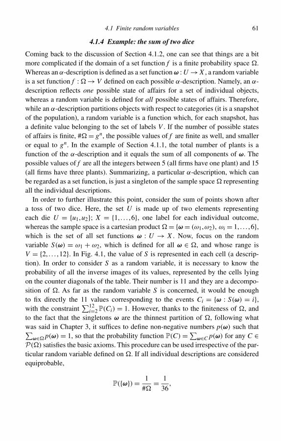
4.1 Finite random variables 61
4.1.4 Example: the sum of two dice
Coming back to the discussion of Section 4.1.2, one can see that things are a bitmore complicated if the domain of a set function f is a finite probability space �.Whereas an α-description is defined as a set function ω : U → X , a random variableis a set function f : � → V defined on each possible α-description. Namely, an α-description reflects one possible state of affairs for a set of individual objects,whereas a random variable is defined for all possible states of affairs. Therefore,while an α-description partitions objects with respect to categories (it is a snapshotof the population), a random variable is a function which, for each snapshot, hasa definite value belonging to the set of labels V . If the number of possible statesof affairs is finite, #� = gn, the possible values of f are finite as well, and smalleror equal to gn. In the example of Section 4.1.1, the total number of plants is afunction of the α-description and it equals the sum of all components of ω. Thepossible values of f are all the integers between 5 (all firms have one plant) and 15(all firms have three plants). Summarizing, a particular α-description, which canbe regarded as a set function, is just a singleton of the sample space � representingall the individual descriptions.
In order to further illustrate this point, consider the sum of points shown aftera toss of two dice. Here, the set U is made up of two elements representingeach die U = {u1,u2}; X = {1, . . . ,6}, one label for each individual outcome,whereas the sample space is a cartesian product � = {ω = (ω1,ω2), ωi = 1, . . . ,6},which is the set of all set functions ω : U → X . Now, focus on the randomvariable S(ω) = ω1 + ω2, which is defined for all ω ∈ �, and whose range isV = {2, . . . ,12}. In Fig. 4.1, the value of S is represented in each cell (a descrip-tion). In order to consider S as a random variable, it is necessary to know theprobability of all the inverse images of its values, represented by the cells lyingon the counter diagonals of the table. Their number is 11 and they are a decompo-sition of �. As far as the random variable S is concerned, it would be enoughto fix directly the 11 values corresponding to the events Ci = {ω : S(ω) = i},with the constraint
∑12i=2 P(Ci) = 1. However, thanks to the finiteness of �, and
to the fact that the singletons ω are the thinnest partition of �, following whatwas said in Chapter 3, it suffices to define non-negative numbers p(ω) such that∑
ω∈� p(ω) = 1, so that the probability function P(C) =∑ω∈C p(ω) for any C ∈P(�) satisfies the basic axioms. This procedure can be used irrespective of the par-ticular random variable defined on �. If all individual descriptions are consideredequiprobable,
P({ω}) = 1
#�= 1
36,
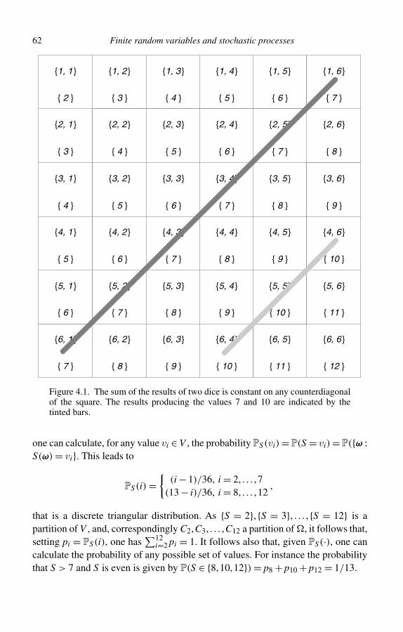
62 Finite random variables and stochastic processes
{ 2 }
{2, 1}
{1, 1} {1, 2} {1, 3} {1, 4} {1, 6}
{ 3 } { 4 } { 5 } { 6 } { 7 }
{ 8 }
{ 9 }
{ 10 }
{ 11 }
{ 12 }
{2, 2} {2, 3} {2, 4} {2, 5}
{1, 5}
{2, 6}
{3, 6}
{4, 6}
{5, 6}
{6, 6}
{ 3 } { 4 } { 5 } { 6 } { 7 }
{3, 1} {3, 2} {3, 3} {3, 4} {3, 5}
{ 4 } { 5 } { 6 } { 7 } { 8 }
{4, 1} {4, 2} {4, 3} {4, 4} {4, 5}
{ 5 } { 6 } { 7 } { 8 } { 9 }
{5, 1} {5, 2} {5, 3} {5, 4} {5, 5}
{ 6 } { 7 } { 8 } { 9 } { 10 }
{6, 1} {6, 2} {6, 3} {6, 4} {6, 5}
{ 10 } { 11 }{ 7 } { 8 } { 9 }
Figure 4.1. The sum of the results of two dice is constant on any counterdiagonalof the square. The results producing the values 7 and 10 are indicated by thetinted bars.
one can calculate, for any value vi ∈ V , the probability PS(vi) = P(S = vi) = P({ω :S(ω) = vi}. This leads to
PS(i) ={
(i − 1)/36, i = 2, . . . ,7(13 − i)/36, i = 8, . . . ,12
,
that is a discrete triangular distribution. As {S = 2}, {S = 3}, . . . ,{S = 12} is apartition of V , and, correspondingly C2,C3, . . . ,C12 a partition of �, it follows that,setting pi = PS(i), one has
∑12i=2 pi = 1. It follows also that, given PS(·), one can
calculate the probability of any possible set of values. For instance the probabilitythat S > 7 and S is even is given by P(S ∈ {8,10,12}) = p8 + p10 + p12 = 1/13.
4.1 Finite random variables 63
4.1.5 The mathematical expectation
For a numerical random variable, X, the mathematical expectation is defined as
E(X ) =∑ω∈�
X (ω)P(ω). (4.6)
As PX (vi) = P({ω : X (ω) = vi} =∑ω∈CiP(ω), and X (ω) = vi, for ω ∈ Ci, the
terms in the sum can be grouped
E(X ) =∑ω∈�
X (ω)P(ω) =g∑
i=1
∑ω∈Ci
X (ω)P(ω) =g∑
i=1
viPX (vi). (4.7)
Note that in (4.6) all the contributions X (ω) coming from any point ω weighted bytheir probability P(ω) are added, whereas in (4.7) all the values v1, weighted bytheir probability PX (vi) are added. In general, in order to have a finite expectation,it is necessary to assume that ∑
ω∈�
|X (ω)|P(ω) < ∞,
but, in the finite case, the expectation (4.6) always exists (it is the sum of a finite num-ber of finite terms). Note that E(X ) is sometimes written as µX , or even µ if there isno doubt about the random variable to which it refers. The mathematical expectationis analogous to the concept of centre of mass for a set of points on a line, where vi isthe coordinate of the ith particle and pi = PX (vi) is its fraction of the total mass. If avalue dominates, that is pj 1, the expectation is close to vj, while if all values havethe same probability, the expectation coincides with the arithmetic mean. Severaluseful variables can be defined starting from the mathematical expectation.
Now, consider an ordinary function g : R → R of a real variable. As an exam-ple, consider the following case: Y = X 2. If the values of X are the five integers{−2,−1,0,1,2}, the values of Y will be the three integers {0,1,4}. The inverseimage of Y = 0 is X = 0, but the inverse image of Y = 1 contains the two eventsX = −1 and X = 1, and the inverse image of Y = 4 contains X = −2 and X = 2, sothat PY (0) = PX (0), PY (1) = PX (−1)+PX (1), and PY (4) = PX (−2)+PX (2). Inother words, Y = g(X ) is a new random variable. The following equality definesY as a random variable Y : � → R
Y (ω) = g(X (ω)) ω ∈ �. (4.8)
Given a finite random variable X assuming gX values, the values of Y = g(X ) willbe gY ≤ gX . If VY is the space of possible values vY ,j for Y , one can derive theprobability distribution PY (·) defined on the measurable space 〈VY ,P(VY )〉 from a
64 Finite random variables and stochastic processes
knowledge of the distribution PX (·) and of the inverse image with respect to g forany value vY ,j
PY (vY ,j) =∑
vX ,i∈g−1(vY ,j)
PX (vX ,i); (4.9)
then, from a knowledge of the probability of singletons, one can obtain the proba-bility for any set belonging to P(VY ), using Equation (4.2). Therefore, the triplet〈VY ,P(VY ),PY 〉 is a probability space.
From Equations (4.7) and (4.9), one has that
E[g(X )] = E(Y ) =∑
vY ,j∈VY
vY ,jPY (vY ,j) =∑
vX ,i∈VX
g(vX ,i)PX (vX ,i). (4.10)
The result presented in (4.10) is known as the fundamental theorem of mathemat-ical expectation. The above discussion shows that there are no major problems inderiving it for the case of finite random variables, whereas in the general case onehas to assume that ∑
vX ,i∈VX
|g(vX ,i)|PX (vX ,i) < ∞,
meaning that there is absolute convergence of the sum (integral). Returning to thesimple example presented above, assume that each of the 5 values of X has thesame probability PX (−2) = PX (−1) = PX (0) = PX (1) = PX (2) = 1/5; this meansthat PY (0) = 1/5 and PY (1) = PY (4) = 2/5.
4.1.6 The variance
As an important application of the fundamental theorem of mathematical expec-tation, one can define the variance of a numerical random variable, X , as themathematical expectation of the squared deviations from E(X )
V(X ) = E[(X −E(X ))2] =∑ω∈�
(X (ω)−E(X ))2P(ω). (4.11)
It turns out that
V(X ) = E(X 2)−[E(X )]2, (4.12)
and this equality is discussed in Exercise 4.3. Note that V(X ) is non-negative,and it is zero only for degenerate (deterministic) distributions. Statisticians usuallydenote V(X ) by σ 2
X . The concept of variance is similar to the mechanical concept of
4.1 Finite random variables 65
moment of inertia with respect to the centre of mass. The square root of the varianceis the standard deviation, σX , a measure of the dispersion for the probability massaround the mathematical expectation.
4.1.7 Covariance and correlation
Given two random variables X and Y defined on the same probability space, theircovariance is defined as
C(X ,Y ) = E[(X −E(X ))(Y −E(Y ))]. (4.13)
When working with more than one random variable, it is useful to introduce theconcept of joint distribution. Now, the constituents of the algebra are the eventsCi,j = {ω : X (ω) = vX ,i,Y (ω) = vY ,j}. The range of the joint random variable is thecartesian product VX ×VY . The joint distribution of the random variables X and Y is
PX ,Y (vX ,i,vY ,j) = P(X −1(vX ,i)∩ Y −1(vY ,j))
= P(X = vX ,i,Y = vY ,j) = P({ω : X (ω) = vX ,i,Y (ω) = vY ,j}),(4.14)
and on subsets AX ×AY of VX ×VY , as a consequence of (4.2), one immediately gets
PX ,Y (AX × AY ) =∑
vX ,i∈AX
∑vY ,j∈AY
PX ,Y (vX ,i,vY ,j). (4.15)
Again, the singletons {(vX ,i,vY ,j)} are a partition of VX × VY , therefore∑vX ,i∈VX
∑vY ,j∈VY
PX ,Y (vX ,i,vY ,j) = 1.
From the theorem of total probability, it is true that
PX (vX ,i) =∑
vY ,j∈VY
PX ,Y (vX ,i,vY ,j) (4.16)
and
PY (vY ,j) =∑
vX ,i∈VX
PX ,Y (vX ,i,vY ,j) (4.17)
are probability distributions, as well. They are called marginal distributions of Xand Y , respectively.
This construction can be extended to any number n of random variables definedon the same probability space, and it will be useful in defining stochastic processes.
66 Finite random variables and stochastic processes
It is possible to use Equation (4.14) in computing (4.13). Using the properties ofexpectation (see Exercise 4.2), one gets
C(X ,Y ) = E[(X −E(X ))(Y −E(Y ))] = E(XY )−E(X )E(Y ). (4.18)
The mathematical expectation of the product XY can be computed by means ofPX ,Y (·, ·) as
E(XY ) =∑
vX ,i∈VX
∑vY ,j∈VY
vX ,ivY ,jPX ,Y (vX ,i,vY ,j).
Auseful quantity related to covariance is the Bravais–Pearson correlation coefficientρX ,Y . It is defined as
ρX ,Y = C(X ,Y )
σX σY. (4.19)
It is possible to prove that −1 ≤ρX ,Y ≤ 1 and this proof is left to the reader as a usefulexercise. If ρX ,Y = −1, the random variables X and Y are perfectly anti-correlated;if ρX ,Y = 1, they are perfectly correlated. The two random variables are calleduncorrelated if ρX ,Y = 0, meaning that C(X ,Y ) = 0 and that E(XY ) = E(X )E(Y ).
It is important to remark that, even if ρX ,Y �= 0, this does not mean that X is acause of Y or vice versa. In other words the presence of correlation between tworandom variables does not imply a causal relationship between the variables. Theremight be a common cause, or the correlation might be there by mere chance. Thisproblem often arises in statistical analyses in the social sciences when the chainsof causation among possibly relevant variables are far from clear; this has alreadybeen discussed at length by John Stuart Mill in his 1836 methodological essay Onthe Definition of Political Economy and the Method of Investigation Proper to It [1].
Two random variables X and Y defined on the same probability space are inde-pendent if all the events X −1(AX ) and Y −1(AY ) are independent. In particular, thismeans that
PX ,Y (vX ,i,vY ,j) = P(X −1(vX ,i)∩ Y −1(vY ,j))
= P(X −1(vX ,i))P(Y −1(vY ,j)) = PX (vX ,i)PY (vY ,j). (4.20)
In other words, if X and Y are independent the joint probability distribution has anice factorization in terms of the product of two marginal distributions. Therefore,for independent random variables it turns out that E(XY )=E(X )E(Y ). Independentrandom variables are uncorrelated and their covariance C(X ,Y ) vanishes. Theconverse is not true: not all uncorrelated random variables are independent!
4.1 Finite random variables 67
4.1.8 Example: indicator functions
The simplest random variable is the so-called event indicator function. It transformscategorical (qualitative) random variables into numerical random variables. Let Abe an event A ∈ F and ω an element of �. The indicator function IA(ω) is
IA(ω) ={
1 if ω ∈ A
0 otherwise.(4.21)
The indicator function has the following properties; let A and B be two events, thenone has:
1. (Indicator function of intersection)
IA∩B(ω) = IA(ω)IB(ω); (4.22)
2. (Indicator function of union)
IA∪B(ω) = IA(ω)+ IB(ω)− IA(ω)IB(ω); (4.23)
3. (Indicator function of complement)
IAc(ω) = 1 − IA(ω); (4.24)
4. (Expectation)
E[IA(ω)] = P(A); (4.25)
5. (Variance)
V[IA(ω)] = P(A)(1 −P(A)). (4.26)
These properties will be proved in Exercise 4.4.
4.1.9 Example: probability of the union of n sets
An immediate consequence of properties (4.22), (4.23) and (4.24) of the indicatorfunction is the theorem giving the probability of the union of two sets. It sufficesto take the expectation of (4.23), use (4.24) and (4.22), to get
P(A ∪ B) = P(A)+P(B)−P(A ∩ B);
this proof is much easier and handier than the one presented in Section 3.6.6.The extension to three sets is based on the associative properties of unions and
68 Finite random variables and stochastic processes
intersections. First of all, one has
IA∪B∪C = I(A∪B)∪C = IA∪B + IC − IA∪BIC
= IA + IB − IAIB + IC − (IA + IB − IAIB)IC
= IA + IB + IC − IAIB − IAIC − IBIC + IAIBIC ,
leading to (after taking the expectation)
P(A ∪ B ∪ C) = P(A)+P(B)+P(C)
−P(A ∩ B)−P(A ∩ C)−P(B ∩ C)+P(A ∩ B ∩ C). (4.27)
Equation (4.27) generalizes to
P(∪ni=1Ai) =
n∑i=1
P(Ai)−∑i �=j
P(Ai ∩ Aj)
+∑
distinct i,j,k
P(Ai ∩ Aj ∩ Ak)− . . .±P(∩ni=1Ai). (4.28)
This result is also known as the inclusion–exclusion formula.
4.1.10 Example: the matching problem
At a party there are n married couples and men and women are randomly pairedfor a dance. A matching occurs if a married couple is paired by chance. What isthe probability of one matching? And what about two? This is an old problem inprobability theory and it is usually referred to as the Montmort’s matching problemas it was first considered by the French mathematician Pierre-Rémond de Montmortactive in the early days of probability theory. His book Essay d’analyse sur les jeuxd’hazard appeared in 1708 [2].
To fix the ideas, let women be labelled from 1 to n, so that V = {1, . . . ,n} is theset of labels. Then men are chosen at random and each man is represented by arandom variable Xi where the subscript i refers to the fact that he is married towoman i. Then Xi = j means that the man married to the ith woman will dance withthe jth woman. One has a match when Xi = i. For instance, if n = 3 couples, one hasV = {1,2,3} and there are n! = 3! = 6 possible couplings (constituents). They are
1. (X1 = 1,X2 = 2,X3 = 3) corresponding to 3 matchings;2. (X1 = 1,X2 = 3,X3 = 2), (X1 = 3,X2 = 2,X3 = 1) and (X1 = 2,X2 = 1,X3 = 3)
corresponding to 1 matching;3. (X1 = 2,X2 = 3,X3 = 1) and (X1 = 3,X2 = 1,X3 = 2) corresponding to no
matchings.
4.1 Finite random variables 69
If the random variable Nn is introduced, representing the number of matchings overany permutation, the case n = 3 is described by the distribution P(N3 = 0) = 2/6 =1/3, P(N3 = 1) = 3/6 = 1/2, P(N3 = 2) = 0 and P(N3 = 3) = 1/6, where thefollowing equation is used to determine the matching probability
P(Nn = k) = bn(k)
n! , (4.29)
and where, for ease of notation, the following position is established
bn(k) = # {Nn = k}. (4.30)
The total number of couples is n!, a rapidly growing function of n. Therefore, thedirect enumeration method soon becomes impractical. What can be said in the gen-eral case? One can immediately observe that P(Nn = n − 1) must be 0; in fact, ifthere are n − 1 matchings the remaining couple must match as well. This fact issometimes referred to as the pigeonhole principle. If attention is fixed on the eventX1 = 1, meaning that the first couple is matched and one is not interested in whathappens to the other couples, one has that
P(X1 = 1) = (n − 1)!n! = 1
n; (4.31)
indeed, if the first husband is paired with his wife, there are still n − 1 availableplaces that can be filled in (n − 1)! ways. Note that this probability is the same forany of the n events {Xi = i}. Similarly, imposing X1 = 1 and X2 = 2 leads to
P(X1 = 1,X2 = 2) = (n − 2)!n! = 1
n
1
n − 1; (4.32)
note that P(X1 = 1,X2 = 2) > P(X1 = 1)P(X2 = 2) meaning that the two eventsare not independent and positively correlated. Again this probability is the samefor any event of the kind {Xi = i,Xj = j} with i �= j. The total number of theseevents is given by the number of ways two objects can be chosen out of n, that isn!/(2!(n − 2)!). In general, for k < n − 1, one can write
P(X1 = 1,X2 = 2, . . . ,Xk = k) = (n − k)!n! = 1
n
1
n − 1· · · 1
n − k + 1; (4.33)
The number of events of this kind is given by n!(k!(n− k)!) as one has to choose kplaces out of n. Due to the pigeonhole principle, the event {X1 = 1, . . . ,Xn−1 = n−1}coincides with {X1 = 1, . . . ,Xn = n} which is only one case over n! and one finds that
P(X1 = 1, . . . ,Xn = n) = 1
n! . (4.34)
70 Finite random variables and stochastic processes
The event {Nn > 0} means that there is at least one matching. It is the union ofevents of the kind {Xi = i}. In symbols
{Nn > 0} = ∪ni=1{Xi = i}. (4.35)
Using the inclusion–exclusion formula (4.28) and the fact that the probabilities ofthe intersections with the same number of sets coincide, one gets
P(Nn > 0) = P(∪n
i=1{Xi = i})= nP(X1 = 1)−
(n
2
)P(X1 = 1,X2 = 2)± . . .
+ (−1)n−1P(X1 = 1, . . . ,Xn = n)
= 1 − 1
2! ± . . . (−1)n−1 1
n! , (4.36)
and the probability of derangements (no matchings) is
P(Nn = 0) = 1 −P(Nn > 0) =n∑
i=0
(−1)i
i! . (4.37)
Note that
limn→∞P(Nn > 0) = 1 − e−1, (4.38)
and
limn→∞P(Nn = 0) = e−1, (4.39)
a somewhat paradoxical result meaning that when n diverges, the probability ofat least one matching does not vanish but remains positive and quite large (morethan 63%). Equation (4.37) can be used to find the probability of the generic event{Nn = k}. From Equations (4.29), (4.30) and (4.37) one gets
bn(0) = n!n∑
i=0
(−1)i
i! . (4.40)
If there are k matchings, there are bn−k(0) possible derangements in the remainingn − k places. The positions of the k matchings can be chosen in n!/(k!(n − k)!)ways. Therefore, the number of ways of obtaining 0 < k ≤ n matchings is
bn(k) = n!k!(n − k)!bn−k(0) = n!
k!(n − k)!(n − k)!n−k∑i=0
(−1)i
i! = n!k!
n−k∑i=0
(−1)i
i! ,
(4.41)
4.1 Finite random variables 71
and, from (4.29), the probability distribution of Nn is
P(Nn = k) = bn(k)
n! = 1
k!n−k∑i=0
(−1)i
i! . (4.42)
Note that Equation (4.42) correctly implies P(Nn = n − 1) = 0 in agreement withthe previous discussion.
4.1.11 Categorical and numerical random variables
It is now due time to reconsider what was established in the previous chaptersin the light of the abstract notion of a random variable. Returning to our samplespace � = {ω = (ω1, . . . ,ωn)}, where n elements are classified into g categories, foreach i = 1, . . . ,n, it is possible to define a function Xi : � → V = {1, . . . ,g} so thatXi(ω) = ωi. If the ith element of ω belongs to the jth category, one has Xi(ω) = j.Note that Xi depends only on the state of the ith individual. It follows that, for eachdescription belonging to the event A(i)
j , Xi = j is observed. In this way, the resultsof Chapter 3, developed there in terms of events, can be translated into the moreelegant language of random variables. Usually, Xi = j is considered as an event(without writing {Xi = j}), and the intersection is represented by a comma, so thatP(X1 = i,X2 = j) denotes the probability of {X1 = i}∩ {X2 = j}.
The set function Xi decomposes � into g sets {A(i)1 , . . . ,A(i)
g }, defined as A(i)j ={ω :
Xi(ω) = j}, which is the inverse image of the set {j} ⊂ V = {1, . . . ,g}. Therefore theset function Xi is a random variable if, for every singleton belonging to {1, . . . ,g},one knows P(A(i)
j ) = P({ω : Xi(ω) = j}), and sets PXi({j}) = P(Xi = j) = P(A(i)j ).
For any subset B of V , the usual construction leads to PXi(B) =∑j∈B PXi({j}) =∑j∈B P({ω : Xi(ω) = j}).The singleton {ω} = A(1)
ω1 ∩ A(2)ω2 ∩ . . . ∩ A(n)
ωn can be more easily referred to asX1 = ω1,X2 = ω2, . . . ,Xn = ωn, taking into account that the set {ω : X1(ω) =ω1,X2(ω) = ω2, . . . ,Xn(ω) = ωn} is nothing other than the singleton defined by theintersection A(1)
ω1 ∩ A(2)ω2 ∩ . . . ∩ A(n)
ωn . Therefore, the inverse image of the sequenceof all individual random variables is the most elementary event one can consider.Given this one-to-one correspondence, one can forget about the �-space and workdirectly on sequences of individual random variables. Then, one writes X1 instead ofX1(ω), always keeping in mind that the meaning of P(Xi = j) is P({ω : Xi(ω) = j}).In other words, a knowledge of P(Xi = j) is equivalent to a knowledge of theprobability of the state of affairs where Xi(ω) = j.
If labels denote categories, the only advantage of the previous discussion issimplicity. Indeed, for individual descriptions, the values of Xi are nothing other thanthe components of the elementary descriptions. However, using indicator functions
72 Finite random variables and stochastic processes
for individual random variables IXi=j(ω), one gets a formal definition for the newrandom variable frequency of the ith category
Ni(ω) =n∑
j=1
IXj=i(ω). (4.43)
4.1.12 Discrete and continuous random variables
In the following, in the case of large systems, the limiting distributions will beapproximated by countable discrete or continuous distributions. In the case ofdiscrete random variables there is no problem in probabilizing all the subsetsof a countable set, and many formulae presented above can be straightforwardlyextended by replacing n with ∞ and assuming that the corresponding series con-verge. However, as discussed at the end of Chapter 3, one must replace finiteadditivity with countable additivity, so that events such as ∪∞
i=1Ai exist and thistransforms a Boolean lattice into a σ -algebra. As mentioned above, in the case ofdiscrete random variables nothing else changes, as in terms of some probabilitydistribution P(k) ≥ 0,
∑∞k=1 P(k) = 1 all the subsets of N have a definite probabil-
ity satisfying the axioms. In this book, countable random variables will be used asa convenient tool to describe finite, even if large, systems.
There are more difficulties in dealing with continuous random variables. It ispossible to show that not all the subsets of R are measurable and one is obligedto consider classes of measurable subsets such as the so-called Borel σ -algebra,which is the smallest σ -algebra containing all subsets of R of the kind (−∞,a].Therefore, in the triplet 〈R,F ,PX 〉, defining a probability space on the image ofa real random variable X , F usually coincides with the Borel σ -algebra B. Thecumulative distribution FX (x) becomes a (piecewise) continuous function and inthe cases in which its first derivative exists, one can define the so-called probabilitydensity function
pX (x) = dFX
dx, (4.44)
and it turns out that
FX (x) =∑u≤x
pX (u) =∫ u
−∞pX (u)du, (4.45)
∑x∈R
pX (x) =∫ +∞
−∞pX (x)dx = 1, (4.46)
where the two notations (sum and integral) will be used in the following as conve-nient. Incidentally, the expectation for a continuous random variable with density
4.2 Finite stochastic processes 73
can be written as
E(X ) =∑x∈R
xpX (x) =∫ +∞
−∞xpX (x)dx < ∞. (4.47)
4.2 Finite stochastic processes
As discussed in Section 4.1.11, an elementary state of affairs is described by {Xi :i = 1, . . . ,n}, a finite sequence of individual random variables whose range (or statespace) is discrete as Xi ∈ {1, . . . ,g}. In general, the labels {1, . . . ,g} are interpretedas categories and expressions such as X1 + X2, or 3X1 are meaningless.
The sequence {Xi : i = 1, . . . ,n} is a simple instance of a stochastic process. Ingeneral a stochastic process is a family of random variables {Xi ∈ S, i ∈ I} definedon the same probability space 〈�,F ,P〉, where S is called the state space, and I isa set of indices. The state space can be discrete (finite or countable) or continuous,and the set of indices can be discrete or continuous as well. When the value of theindex i is fixed, Xi is a random variable, and P(Xi ∈ A) means the probability thatthe ith value of X belongs to some subset of S. When a point of the sample spaceis fixed, the stochastic process becomes an ordinary function of the index set I .
In the case relevant to the present book, the state space is the range of theindividual random variables, i.e. the labels {1, . . . ,g}, and the set of indices aregiven by the integers from 1 to n: I = {1, . . . ,n}.
The notation X(n)= (X1,X2, . . . ,Xn) usually denotes a random vector, interpretedas a sequence of random variables; a sequence of specific values assumed by theserandom variables is represented by x(n)= (x1,x2, . . . ,xn); the probability of the eventX(n) = x(n), that is (X1 = x1, . . . ,Xn = xn), is P(X(n) = x(n)) = pX1,...,Xn(x1, . . . ,xn) =pX(n) (x(n)); the function pX1,...,Xn(x1, . . . ,xn) is called n-point finite dimensionaldistribution. The probability space of the events X(n) = x(n) is finite, and theprobability of all the constituents must be fixed, that is pX(n) (x(n)) : pX(n) (x(n)) ≥0,∑
x∈�(x) pX(n) (x(n)) = 1, where the symbol �(x) is used for the set of all pos-sible elementary outcomes for n joint individual observations. The cardinality of�(x) is given by #�(x) = gn, as there is a one-to-one mapping between the set� of individual descriptions, and �(x). As was discussed in the previous chapter,one can use either the absolute or the predictive method to assign the probabilitiespX1,...,Xn(x1, . . . ,xn).
As the index set I is usually infinite, a full characterization of the stochastic pro-cess is possible if all the finite dimensional distributions are known for all xi ∈ S andfor any integer n > 0. This is a consequence of Kolmogorov’s extension theorem. Itturns out that the knowledge of all the finite dimensional distributions is sufficientfor the existence of a stochastic process, even if I is a continuous set of indices.
74 Finite random variables and stochastic processes
Coming back to the simple case in which I = {1, . . . ,n}, and S is a finite set oflabels {1, . . . ,g}, the full characterization of the n-step processes is given by theknowledge of the m-point finite dimensional distributions with 1 ≤ m ≤ n: pX1(x1),pX1,X2(x1,x2), . . ., pX1,...,Xm(x1, . . . ,xm), . . ., pX1,...,Xn(x1, . . . ,xn). These probabilityfunctions must satisfy Kolmogorov’s compatibility conditions. The first conditionis a consequence of the symmetry property of intersections in a Boolean algebra,
pX1,...,Xm(x1, . . . ,xm) = pXi1 ,...,Xim(xi1 , . . . ,xim), (4.48)
where i1, . . . , im is any of the m! possible permutations of the indices. The secondcondition is a consequence of the finite additivity axiom A3,
pX1,...,Xm(x1, . . . ,xm) =∑
xm+1∈S
pX1,...,Xm,Xm+1(x1, . . . ,xm,xm+1). (4.49)
Kolmogorov’s compatibility conditions may seem trivial, but they are used ashypotheses in Kolmogorov’s extension theorem quoted above. These conditionsare automatically satisfied if the finite dimensional distributions are built using thepredictive method. As a consequence of the multiplication theorem, one has
pX1,...,Xm(x1, . . . ,xm) = P(X1 = x1, . . . ,Xm = xm)
= P(X1 = x1)P(X2 = x2|X1 = x1) . . .
P(Xm = xm|X1 = x1, . . . ,Xm−1 = xm−1). (4.50)
Hence, a stochastic process is often characterized in terms of the predictive lawP(Xm = xm|X1 = x1, . . . ,Xm−1 = xm−1) for any m > 1 and of the ‘initial’distributionP(X1 = x1). The predictive probability has only to fulfil the probability axioms:P(Xm = xm|X(m−1) = x(m−1)) ≥ 0, and
∑xm∈S P(Xm = xm|X(m−1) = x(m−1)) = 1.
In other words, one has to fix the probability of the ‘next’ observation as a functionof all the previous results. Predictive laws which are simple functions of xm andx(m−1) are particularly interesting.
4.2.1 Sampling stochastic processes
Stochastic processes defined by means of a predictive law have many applicationsin physics, genetics, economics and the natural sciences, as they naturally repre-sent probabilistic mechanisms evolving in time. The simplest physical model isrepresented by coin (or die) tossing, or by the game of roulette; in all these casesthe ‘random’device produces sequences of values. The predictive probability takesinto account the properties of the device and all the previous results, in order toassess the probability for the next trial. In the framework of stochastic processes,
4.2 Finite stochastic processes 75
a sample is nothing other than the initial part of a sequence, and does not coincidewith the intuitive notion of the part of a whole (the sampled population). On theother side, in statistics sampling is in a strict sense a partial observation of somepopulation. Its physical model is drawing balls from an urn. In this second frame-work, the only property of the random device is just the set of balls in the urn: itscomposition with respect to the variates of interest. The probability of an outcomemay depend on the previous results, but, first of all, it depends on the compositionn = (n1, . . . ,ng) of the urn, where ni is the number of objects belonging to the ithcategory. The simplest example is the draw without replacement from an urn ofknown composition; in this case, the finite dimensional distributions must satisfythe ‘final constraint’ that X(n) has the frequency vector n describing the composi-tion of the urn. This problem has already been discussed in Chapter 2 as a countingproblem and in Chapter 3 as a probabilistic urn problem. In the following sections,the main results of Chapter 3 will be re-written in the language of random variables,analyzed in terms of the possible compositions of the population.
4.2.2 n-Exchangeable random processes
The hypergeometric process
The physical process of drawing balls without replacement at random and froman urn of given composition n = (n1, . . . ,ng) can be described by the followingformal stochastic process. Note that the state space {1, . . . ,g} denotes the g differentcolours present in the urn. Consider a sequence of individual random variablesX1, . . . ,Xn whose range is the label set {1, . . . ,g} and characterized by the followingpredictive probability:
Pn(Xm+1 = j|X1 = x1, . . . ,Xm = xm) = Pn(Xm+1 = j|m) = nj − mj
n − m. (4.51)
Now, based on the rule (4.51), one can find the probability of the fundamentalsequence X(m)
f = (X1 = 1, . . . ,Xm1 = 1,Xm1+1 = 2, . . .Xm1+m2 = 2, . . . ,Xm−mg+1 =g, . . . ,Xm = g) with m ≤ n balls drawn, of which the first m1 is of colour 1, thefollowing m2 of colour 2, and so on, until the last set of mg balls of colour g, with∑g
i=1 mi = m. By repeated applications of (4.51), one gets
Pn(X(m)f )
= n1
n
n1 − 1
n − 1· · · n1 − m1 − 1
n − m1 − 1
n2
n − m1
n2 − 1
n − m1 − 2· · · n2 − m2 − 1
n2 − m1 − m2 − 1
× ng
n − m + mg
ng − 1
n − m + mg − 1· · · ng − mg − 1
n − m − 1, (4.52)
76 Finite random variables and stochastic processes
a result that can be written in a more compact form as
Pn(X(m)f ) = (n − m)!
n!g∏
i=1
ni!(ni − mi)! . (4.53)
The nice point about the probability given by Equation (4.53) is that it is the samefor any individual sequence with the sampling vector m, and the number of thesesequences is given by the multinomial factor (see the discussion around Equation(2.8) in Chapter 2); therefore one has
Pn(m) = m!∏gi=1 mi!
Pn(X(m)f ), (4.54)
leading to the hypergeometric sampling distribution
Pn(m) = m!∏gi=1 mi!
(n − m)!n!
g∏i=1
ni!(ni − mi)! =
∏gi=1
(ni
mi
)(
n
m
) . (4.55)
The hypergeometric process discussed above is the simplest case of an n-exchange-able process. A general definition of this important class of stochastic processeswill be given below.
n-Exchangeable processes
Consider again a sequence of individual random variables X1, . . . ,Xn whose rangeis the label set {1, . . . ,g}. As discussed above there are gn possible sequences X1 =x1, . . . ,Xn = xn, whereas the number of possible occupation vectors n = (n1, . . . ,ng)
is given by (n + g − 1
n
). (4.56)
Moreover, given a particular occupation vector n, the number of correspondingindividual sequences X(n) is
n!n1! · · ·ng ! . (4.57)
Thanks to the construction discussed above in this section, the sequence of randomvariables defines a stochastic process. If the finite dimensional probabilities aresuch that, for any integer m = 2, . . . ,n, one has
P(X1 = x1, . . . ,Xm = xm) = P(Xi1 = x1, . . . ,Xim = xm), (4.58)
4.2 Finite stochastic processes 77
for any of the m! possible permutations of the indices, then the stochastic processis called n-exchangeable. Note that condition (4.58) differs from condition (4.48).The meaning of (4.58) is that all the individual sequences corresponding to thesame occupation vector m have the same probability. Therefore, an immediateconsequence of the definition (4.58) and of A3 (finite additivity) is that
P(X(m)) = P(m)
(m!
m1! · · ·mg !)−1
, (4.59)
where a shortcut notation has been used and m is the frequency vector of theparticular random vector X(m) = x(m). Equation (4.59) is compatible with anyprobability distribution on m, {P(m) :
∑P(m) = 1,
∑gi=1 mi = m}. It turns out
that (n + g − 1)!/(n!(g − 1)!) − 1 parameters are needed to completely define theprobability space. They represent the probability of all possible compositions of thepopulation with respect to the g labels (categories). In the urn model, they are allthe possible compositions of the urn with respect to g colours. Given that, for anysubsequence, the finite dimensional probability P(Xi1 = x1,Xi2 = x2, . . . ,Xim = xm),ij ≤ n can be obtained by marginalization of P(X1 = x1,X2 = x2, . . . ,Xn = xn) usingthe second compatibility condition (4.49), it follows that all the finite dimensionalprobabilities are known if P(n) is known. The resulting predictive law has someinteresting properties:
1. the past evidence X(m) can be replaced by its frequency vector m,
P(Xm+1 = i|X(m)) = P(Xm+1 = i|m) = p(i,m); (4.60)
2. the event Xm+2 = i,Xm+1 = j and the symmetrical one Xm+2 = j,Xm+1 = i areequiprobable given any evidence:
P(Xm+2 = i,Xm+1 = j|m) = P(Xm+2 = j,Xm+1 = i|m). (4.61)
Exchangeable processes as mixtures of hypergeometric processes
The hypergeometric process defined above is not extendible to n + 1 steps. If themodel urn contains n balls, the process stops at the nth step. If the individual vectorX(n) defines a sequence whose length is n steps, from Equation (4.53), one has
Pn(X(n)) = 1n!∏g
i=1 ni!, (4.62)
78 Finite random variables and stochastic processes
where the notation highlights the fact that all the sequences are equiprobable. Nowassume that Equation (4.59) is valid also at the nth step, leading to
P(X(n)) = P(n)
n!∏gi=1 ni!
. (4.63)
Equation (4.63) represents a mixture of hypergeometric processes with mixingprobability P(n); indeed, it can be re-written as
P(X(n)) = P(X(n)|n)P(n), (4.64)
with
P(X(n)|n) = Pn(X(n)) = 1n!∏g
i=1 ni!, (4.65)
corresponding to the hypergeometric process. The mixing probability representssampling without replacement from an urn of unknown composition with eachcomposition having probability P(n). Note that a mixture of hypergeometric pro-cesses could be extendible to the next step and even to infinity, as will be clear fromthe examples discussed below. Finally, note that also the converse is true, that is anyn-exchangeable stochastic process can be written as a mixture of hypergeometricprocesses. This is also a consequence of Equation (4.59). This result is known asthe finite version of de Finetti’s representation theorem for exchangeable processesand it will be further discussed in Section 4.3, where a proof in the tradition of theItalian neo-Bayesian school will be presented.
Examples of exchangeable processes
It is now time to consider some specific examples where P(n) is explicitly given.
1. (Hypergeometric process again) As already discussed, the hypergeometric pro-cess follows from (4.63) setting P(n′) = δ(n′,n). The corresponding urn modelis sampling without replacement from an urn whose initial composition is givenby the vector n. A possible accommodation model amounts to choosing freepositions at the instant of accommodation with uniform probability, wheren = (n1, . . . ,ng) is the distribution of the initial available positions. Brillouingave a physical interpretation to such an accommodation model while tryingto derive quantum statistics. He used a geometrical analogy and introduced the‘volume’of a cell and set this volume equal to the ‘positive volume’of fermions,particles subject to Pauli’s exclusion principle. In such an extreme case, where thevolume of a cell and the volume of a particle coincide, no more than one particle
4.2 Finite stochastic processes 79
can enter a cell. In Brillouin’s framework a category (energy level) is made up ofseveral cells. If the ith energy level contains ni cells and mi particles, there is stillroom for no more than ni − mi particles. All sequences with occupation vectordifferent from n are impossible, whereas all the possible individual sequencesare equiprobable. The predictive probability (conditioned on n) in this case is:
Pn(Xm+1 = i|X(m)) = pn(i,mi,m) = ni − mi
n − m, (4.66)
a reformulation of (3.20).2. (Multinomial process) If P(n) is the multinomial distribution, the independent
and identically distributed case follows. To make this clear it is sufficient toreplace (3.8) in (4.59) leading to
P(X(n)) =g∏
i=1
pnii , (4.67)
where ni is the number of Xj = i, that is ni = #{Xj = i, j = 1, . . . ,n}. This coincideswith
P({ω}) =g∏
i=1
pnii , (4.68)
where pi has the same meaning. The corresponding urn model is sampling withreplacement from a Bernoullian urn, whereas the accommodation model is thatof successive accommodations ruled by a probability which is the same for allvariables, and which is independent of the values of all other variables. Indeed,in the i.i.d. case, the predictive probability is:
P(Xm+1 = i|X(m)) = pi, (4.69)
a reformulation of (3.19). One must choose g − 1 probability values, given that{pi ≥ 0,
∑gi pi = 1}.
3. (Pólya process) The Pólya process follows from (4.59) setting
P(n) = Polya(n;α) = n!α[n]
g∏i=1
α[n]i
ni! , (4.70)
where α = (α1, . . . ,αn) is a vector of parameters, α =∑gi=1 αi and α[n] is the
Pochhammer symbol representing the rising (or upper) factorial defined by
α[n] = α(α + 1) · · ·(α + n − 1). (4.71)
The urn model for the Pólya process is sampling with replacement and unitaryprize from an urn whose initial composition is α = (α1, . . . ,αg). In this case, the
80 Finite random variables and stochastic processes
predictive probability is
Pα(Xm+1 = i|X(m)) = pα(i,mi,m) = αi + mi
α + m. (4.72)
The corresponding accommodation model is choosing each category i withprobability proportional with αi + mi, αi being the initial ith weight, and mi
the number of objects already accommodated in that category. Based on thisproperty, Brillouin created the geometrical interpretation of ‘negative volume’for bosons, as their presence increases the ‘volume’ of the cell they belongto. Observe that (4.72) is meaningful also for a vector α of negative integerparameters, provided mi ≤ |αi|, in which case |αi| represents the number of‘positions’ available to the ith category, or the initial number of balls of colouri. In other words, one can set ni = |αi|, n = |α| and (4.72) coincides with (3.20),in symbols pn(·) = pα=−n(·). Further note that, in the limit αj → ∞, αj/α = pj,formula (4.72) becomes (3.19). This means that, within the realm of exchange-able sequences, the predictive form (4.72) encompasses both independent and(both positively and negatively) correlated sequences, corresponding to simpleurn models as well as to (both positively and negatively) correlated accommo-dation models. This family of sequences can be characterized by the invarianceof the heterorelevance coefficient, a notion introduced by Keynes in his Treatiseon Probability (see the references of Chapter 1). The notion of invariance forheterorelevance coefficients is due to Costantini. Given its importance, the Pólyaprocess will be studied in greater detail in Chapter 5.
4.2.3 Example: bingo and conditioning
The game of bingo is based on the sequential draw without replacement of all 90numbered balls from an urn. We denote by Xj = i the event that the jth drawn numberis i, i, j = 1, . . . ,n. The game is fair if all 90! sequences which are distinct permuta-tions of {1, . . . ,90} are equiprobable. Therefore, the sequence of random variablesX1,X2, . . . ,X90 defines an exchangeable stochastic process. Do X1 and X90 have thesamedistribution?Fromanaïvepointofviewthe twocases lookquitedifferent, as X1
can take 90 equiprobable values, whereas the possibilities for X90 are restricted to theonly and last ball left in the urn. However, unconditional on the past, the range of X90
just coincides with the range of X1 or of any other variable! It is true that, conditionalon the pasthistory, the rangeof X90 is just the last ball left, but if onearrives justbeforethe last draw and does not know the past history, then P(X90 = i) = P(X1 = i) = 1/90(see also Exercise 3.4).This example is useful in order to better understand the notionof marginal distribution for a random vector. As a consequence of (4.51), the pre-dictive probability for the process X1,X2, . . . ,X90 is P(Xm+1 = i|X1 = x1, . . . ,Xm =xm) = (1−mi)/(90−m), where mi = 0 if X1 �= i, . . . ,Xm �= i, and mi = 1 otherwise.
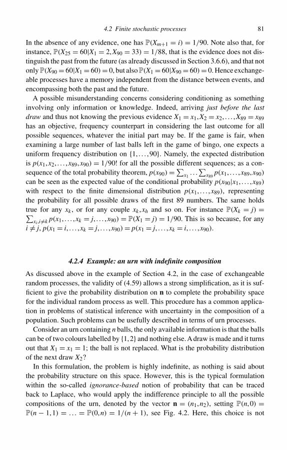
4.2 Finite stochastic processes 81
In the absence of any evidence, one has P(Xm+1 = i) = 1/90. Note also that, forinstance, P(X25 = 60|X1 = 2,X90 = 33) = 1/88, that is the evidence does not dis-tinguish the past from the future (as already discussed in Section 3.6.6), and that notonly P(X90 = 60|X1 = 60) = 0, but also P(X1 = 60|X90 = 60) = 0. Hence exchange-able processes have a memory independent from the distance between events, andencompassing both the past and the future.
A possible misunderstanding concerns considering conditioning as somethinginvolving only information or knowledge. Indeed, arriving just before the lastdraw and thus not knowing the previous evidence X1 = x1,X2 = x2, . . . ,X89 = x89
has an objective, frequency counterpart in considering the last outcome for allpossible sequences, whatever the initial part may be. If the game is fair, whenexamining a large number of last balls left in the game of bingo, one expects auniform frequency distribution on {1, . . . ,90}. Namely, the expected distributionis p(x1,x2, . . . ,x89,x90) = 1/90! for all the possible different sequences; as a con-sequence of the total probability theorem, p(x90) =∑x1
. . .∑
x89p(x1, . . . ,x89,x90)
can be seen as the expected value of the conditional probability p(x90|x1, . . . ,x89)
with respect to the finite dimensional distribution p(x1, . . . ,x89), representingthe probability for all possible draws of the first 89 numbers. The same holdstrue for any xk , or for any couple xk ,xh and so on. For instance P(Xk = j) =∑
xi ,i �=k p(x1, . . . ,xk = j, . . . ,x90) = P(X1 = j) = 1/90. This is so because, for anyi �= j, p(x1 = i, . . . ,xk = j, . . . ,x90) = p(x1 = j, . . . ,xk = i, . . . ,x90).
4.2.4 Example: an urn with indefinite composition
As discussed above in the example of Section 4.2, in the case of exchangeablerandom processes, the validity of (4.59) allows a strong simplification, as it is suf-ficient to give the probability distribution on n to complete the probability spacefor the individual random process as well. This procedure has a common applica-tion in problems of statistical inference with uncertainty in the composition of apopulation. Such problems can be usefully described in terms of urn processes.
Consider an urn containing n balls, the only available information is that the ballscan be of two colours labelled by {1,2} and nothing else. A draw is made and it turnsout that X1 = x1 = 1; the ball is not replaced. What is the probability distributionof the next draw X2?
In this formulation, the problem is highly indefinite, as nothing is said aboutthe probability structure on this space. However, this is the typical formulationwithin the so-called ignorance-based notion of probability that can be tracedback to Laplace, who would apply the indifference principle to all the possiblecompositions of the urn, denoted by the vector n = (n1,n2), setting P(n,0) =P(n − 1,1) = . . . = P(0,n) = 1/(n + 1), see Fig. 4.2. Here, this choice is not
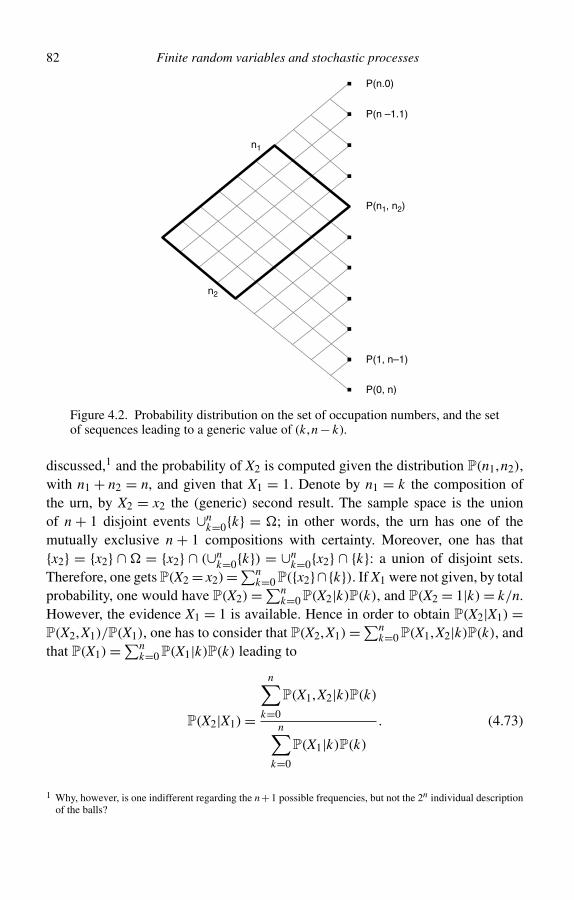
82 Finite random variables and stochastic processes
P(n.0)
P(n –1.1)
n1
n2
P(n1, n2)
P(1, n–1)
P(0, n)
Figure 4.2. Probability distribution on the set of occupation numbers, and the setof sequences leading to a generic value of (k,n − k).
discussed,1 and the probability of X2 is computed given the distribution P(n1,n2),with n1 + n2 = n, and given that X1 = 1. Denote by n1 = k the composition ofthe urn, by X2 = x2 the (generic) second result. The sample space is the unionof n + 1 disjoint events ∪n
k=0{k} = �; in other words, the urn has one of themutually exclusive n + 1 compositions with certainty. Moreover, one has that{x2} = {x2} ∩ � = {x2} ∩ (∪n
k=0{k}) = ∪nk=0{x2} ∩ {k}: a union of disjoint sets.
Therefore, one gets P(X2 = x2) =∑nk=0 P({x2}∩{k}). If X1 were not given, by total
probability, one would have P(X2) =∑nk=0 P(X2|k)P(k), and P(X2 = 1|k) = k/n.
However, the evidence X1 = 1 is available. Hence in order to obtain P(X2|X1) =P(X2,X1)/P(X1), one has to consider that P(X2,X1) =∑n
k=0 P(X1,X2|k)P(k), andthat P(X1) =∑n
k=0 P(X1|k)P(k) leading to
P(X2|X1) =
n∑k=0
P(X1,X2|k)P(k)
n∑k=0
P(X1|k)P(k)
. (4.73)
1 Why, however, is one indifferent regarding the n+1 possible frequencies, but not the 2n individual descriptionof the balls?
4.2 Finite stochastic processes 83
Note that P(X1,X2|k) is the hypothetical probability of the sample, also called con-ditioned sampling distribution by statisticians, whereas P(k) denotes the probabilityof the hypothesis. Note also that the total probability theorem, which can be inter-pretedasaweightedmeanofhypotheticalprobabilities, isusedforbothP(X2,X1)andP(X1) separately. It would be a mistake to write P(X2|X1,k) = P(X2,X1|k)/P(X1|k)
and then to find the expected value of this ratio of conditional probabilities. On thispoint, see the exercise on hypothetical conditional probability below.
In order to determine P(X1|k), and P(X1,X2|k), the type of sampling must bespecified. Assume that X1, . . . ,Xn|k is a hypergeometric process, as the drawn ballsare not replaced. The probabilities of sequences conditioned on the compositionof the urn can be computed. Everybody agrees with the choice P(X1 = 1|k) = k/nif there are k balls of colour 1 over n. The joint conditional probability distri-bution P(X1,X2|k) is given by P(X1,X2|k) = P(X2|X1,k)P(X1|k), and P(X2 =1|X1 = 1,k) = (k − 1)/(n − 1). This intuitive result is in agreement with the pre-dictive probability (4.66). For the absolute method see Exercise 3.4. Hence P(X1 =1) =∑n
k=0 P(X1 = 1|k)P(k) = (n + 1)−1∑nk=0 P(X1 = 1|k), and
∑nk=0 P(X1 =
1|k) =∑nk=0 k/n = (n + 1)/2. In the end, one finds that P(X1 = 1) = 1/2. As for
P(X1 = 1,X2 = 1), one has that P(X1 = 1,X2 = 1)= (n+1)−1∑nk=0 P(X2 = 1,X1 =
1,k), and∑n
k=0 P(X2 = 1,X1 = 1,k) = (n(n − 1))−1∑nk=0(k − 1)k = (n + 1)/3.
Eventually, all these calculations lead to P(X2 = 1|X1 = 1) = P(X2 = 1,X1 = 1)/
P(X1 = 1) = 2/3.The approach used to solve this problem can be summarized as follows:
1. set the probability distribution P(n);2. consider X1, . . . ,Xn|n as a hypergeometric process;3. compute the probability of any event A as
∑n P(A|n)P(n).
The predictive approach in this case is very simple: let us consider (3.25), thepredictive rule used in the example of n energy elements to be divided into 2molecules in Section 3.4.3. Then, setting
P(Xm+1 = 1|X1 = x1, . . . ,Xm = xm) = 1 + m1
2 + m, (4.74)
the distribution of n = (n1,n2) is given by P(n1,n2) = 1/(n + 1) and is uniform.The probability of X1 = 1 is simply 1/2, and that of X2 = 1 given that X1 = 1 is(1 + 1)/(2 + 1) = 2/3.
4.2.5 Example: Laplace’s rule of succession
Laplace’s succession rule is an example of an application for the predictive prob-ability (4.74). The rule states that ‘whenever, in n identical experiments, one has
84 Finite random variables and stochastic processes
observed k successes (and n− k failures), the probability that the next observationis a success is (k + 1)/(n + 2)’. Such a rule is too general and, not surprisingly, itwas already criticized by frequentists in the second half of the nineteenth century.In order to better appreciate Laplace’s line of reasoning, it is useful to follow theroute he used to derive (4.74).
Laplace’s procedure
Assume that the ‘true’ but unknown probability of success is 0 < θ ≤ 1. Then thehypothetical probability of a specific sequence with k successes in n trials is θ k(1−θ)n−k . Then, introduce the a-priori distribution of θ ∈ (0,1]: f (θ) ≥ 0,
∑θ f (θ) = 1.
As a consequence of total probability,∑
θ θk(1 − θ)n−k f (θ) is the probability of aspecific sequence with k successes denoted by the random vector X(n)(k).
Laplace wants to find P(Xn+1 = 1|X(n)(k)), and he introduces the randomvariable � = θ . Now, one has P(Xn+1 = 1|X(n)(k)) = ∑
θ P(Xn+1 = 1,� =θ |X(n)(k)) =∑θ P(Xn+1 = 1|� = θ ,X(n)(k))P(� = θ |X(n)(k)), where
P(Xn+1 = 1|� = θ ,X(n)(k)) = P(Xn+1 = 1|� = θ), (4.75)
because given � = θ the previous results are inessential, and
P(� = θ |X(n)(k)) (4.76)
is the posterior distribution in the hypothesis � = θ after k successes and n − kfailures. It turns out that
P(Xn+1 = 1|� = θ) = θ , (4.77)
as the parameter is equal to the probability of a success, and P(� = θ |X(n)(k)) =P(� = θ |k,n) can be found using Bayes’ theorem:
P(� = θ |X(n)(k)) = AP(X(n)(k)|� = θ)f (θ) = Aθ k(1 − θ)n−k f (θ), (4.78)
where A−1 =∑θ θk(1 − θ)n−k f (θ) is a normalization constant. Note that the pos-terior probability P(θ |X(n)(k)) is a function of θ only. Laplace chooses f (θ) = c, auniform distribution for the random variable �, as a consequence of the indiffer-ence principle applied to all the possible values of the parameter. This assumptionmeans that for any interval (a,b) ⊂ (0,1], P(� ∈ (a,b)) = b − a, and the constantis c = 1. However, for the purpose of deriving the rule of succession, it is sufficientto observe that, being constant, f (θ) cancels from (4.78), and the equation reducesto P(� = θ |X(n)(k)) = A′ · θk(1 − θ)n−k . Before presenting all the mathematicaldetails, note that the evidence transforms the initial flat prior distribution of � ina posterior distribution peaked around θ k/n, and this effect increases with the
4.2 Finite stochastic processes 85
size of the sample. The exact calculation shows that
P(Xn+1 = 1|X(n)(k)) = A′∫ 1
0θ · θk(1 − θ)n−kdθ = 1 + k
2 + n. (4.79)
In other words, the predictive probability of success is equal to the expected valueof θ over the posterior distribution. Laplace applied this formula to the outstandingphilosophical problem introduced by Hume. What is the degree of confidence for thetruth of the sentence the sun will rise tomorrow? Having looked for the evidenceof all successes since the birth of historical reports, Laplace obtained a numberof trials equal to 1,826,213 and all of them successful. Therefore, he could bet1,826,214 : 1 in favour of the sun rising on the next day. If the evidence is large,(k + 1)/(n + 2) k/n, and Laplace’s estimate cannot be distinguished from thefrequency of successes, which frequentists use to assess probability. However, theformula holds also when no evidence is present, a case in which the frequencyinterpretation of probability is meaningless, and this is the main reason for thecriticisms put forward by frequentists.
Jokes against the succession rule
Imagine that somebody is falling from the top floor of the Empire State Building,and passing any floor while falling, he/she observes ‘till now, everything is OK’.The probability of success (survival) at the next floor is increasing, if one appliesthe succession rule. This seems paradoxical, as the falling person will die withprobability very close to 1 when hitting the road surface. A more careful analysisof this paradox reveals that:
1. conditioned on the knowledge of the floor number of the building, the processis deterministic;
2. the process is not exchangeable: once the falling person is dead (failure), he/shecannot be resuscitated.
Another common criticism of inductive inference (and of Laplace’s rule as a methodfor quantitatively assessing it) is as follows. You are a turkey living in the USAand you will be killed just before the next Thanksgiving Day. Since your birth,you have observed that some humans come at regular periods in order to feed you.Every day, your confidence in the success (tomorrow they will come and feed me)is increasing, even if Thanksgiving is approaching. Your problem is that you do notknow anything about Thanksgiving.
4.2.6 Probability of facts/probability of laws
Now compare Laplace’s procedure with the one in Section 4.2.4; the two hypothesesof uniform distributions: P(n,0) = . . . = P(k,n − k) = . . . = P(0,n) = 1/(n + 1)
86 Finite random variables and stochastic processes
and f (θ) = 1, for θ ∈ (0,1] lead to the same predictive probability. Is this merelydue to coincidence? In the first case the probability of the individual descriptionsP(X1 = x1, . . . ,Xm = xm|k,n) follows the hypergeometric distribution. Assume thatn � 1, and introduce the relative frequency θk = k/n ∈ {0,1/n,2/n, . . . ,(n−1)/n,1}.Then the distance between two consecutive points θk+1 − θk = θk = θ = 1/ndecreases as n increases. The set a < k ≤ b, whose probability is (b−a)/(n+1), ismapped into θa < θk ≤ θb. Then P(θa < θk ≤ θb) = (b−a)/(n+1) θb −θa, that isthe continuous uniform distribution in (0,1]. In the limit n → ∞, one can write thatthe random variable θk = k/n converges to the random variable θ : P(c < θ ≤ d) =∫ d
c f (θ)dθ with f (θ) = 1, θ ∈ [0,1].2 Returning to P(X1 = x1, . . . ,Xm = xm|k,n),for n → ∞, it is possible to prove that the hypergeometric distribution convergesto the binomial distribution
P(X1 = x1, . . . ,Xm = xm|k,n) (
k
n
)h(1 − k
n
)m−h
θh(1 − θ)m−h;
this result is easy to understand in terms of urn models. When the sample size nis large and both n1 and n2 are large, there is no difference in the probabilitiesresulting from sampling with replacement and sampling without replacement, as,in practice, removing a few balls does not change the composition of the urn. Inother words, assuming a uniform density on θ , conditioned on which the sampleis i.i.d. (binomial, in this simple case), is equivalent to assuming a uniform prob-ability on the unknown composition (k,n − k), conditioned on which the sampleis hypergeometric. The two methods share the same predictive probability. In thehistory of predictive probabilities, the first route was followed by de Finetti andby subjectivists, whereas the second finitary procedure was used by Johnson, whodid not use Bayesian methods, together with Keynes, Carnap and other supportersof logicism, who tried to avoid the introduction of infinities. Eventually, one couldsay that the finitary predictive characterization of a stochastic process only usesthe probability of facts, that is the probability of the observables Xi or n, whereasthe other method introduces the probability of a hidden variable – the parameter,conditioned on which the variables are i.i.d. – representing the probability of a law.This law (the parameter) becomes a fact only in the infinite limit n → ∞, where itrepresents the value of the relative frequency.
4.3 Appendix 1: a finite version of de Finetti’s theorem
It turns out that all n-exchangeable processes can be represented as mixtures(linear superpositions) of hypergeometric processes. Here, this important result
2 Here one can exchange ( with [, as, for a continuous density, single points have zero probability. Further notethat this result can be made rigorous by introducing the appropriate definition of convergence for a sequence ofrandom variables.
4.3 Appendix 1: a finite version of de Finetti’s theorem 87
due to Bruno de Finetti will be further discussed in the case of a dichotomousn-exchangeable process.
4.3.1 Kolmogorov’s compatibility conditions for a finite dichotomous process
Let us consider a finite (n-step) dichotomous stochastic process. This is a sequenceof n random variables X1, . . . ,Xn each of which can assume one of two values. Forthe sake of simplicity, let us assume that, ∀i, Xi = IA that is Xi = 1 if event A occursat step i and Xi = 0 if event A does not take place at step i.
A stochastic process is fully characterized if all its finite dimensional distribu-tions are given. As discussed above, these distributions must satisfy Kolmogorov’scompatibility conditions. In the simple case under scrutiny, these conditions become
p0 + p1 = 1,
p1,1 + p1,0 = p1, p0,1 + p0,0 = p0,
p1,1,1 + p1,1,0 = p1,1, p0,0,1 + p0,0,0 = p0,0,
. . . , (4.80)
where, e.g., p1,1,1 = P(X1 = 1,X2 = 1,X3 = 1) and the symmetry compatibilityconditions (such as P(X1 = 1,X2 = 1,X3 = 0) = P(X3 = 0,X1 = 1,X2 = 1)) areimplicitly assumed.
4.3.2 Again on exchangeability
An exchangeable finite (n-step) dichotomous stochastic process is a sequence of ndichotomous random variables X1, . . . ,Xn such that the finite dimensional probabil-ities do not depend on the particular order of 0s and 1s, but only on the number of0s and 1s. In other words, for instance, one has p0,0,1 = p0,1,0 = p1,0,0. Notice that,as the sums of the number of 0s and the number of 1s coincide with the number oftrials considered, and Sn =∑n
i=1 Xi coincides with the number of 1s (usually calledthe number of successes), one has for the probability of a particular sequence withh successes out of m ≤ n trials, X1, . . . ,Xm,
P(X1, . . . ,Xm) = P(Sm = h)(m
h
) , (4.81)
as m!/(h!(m − h)!) is the number of sequences with h successes out of m trials.This formula is a specialization of (4.59). It is useful to introduce the new symbolp(m)
h =P(Sm = h).Another useful quantity is ph = p(h)h , the probability of h successes
out of h trials. One has that
ph =m∑
r=h
p(m)r
(r
h
)[(m
h
)]−1
; (4.82)
88 Finite random variables and stochastic processes
in order to prove equation (4.82), one has to count all the possibilities containing hsuccesses in the first h trials. A single sequence with r ≥ h successes out of m trialshas probability
p(m)r(m
r
) ; (4.83)
the number of these sequences is (m − h
r − h
), (4.84)
and h ≤ r ≤ m so that
ph =m∑
r=h
p(m)r
(m − h
r − h
)[(m
r
)]−1
, (4.85)
which coincides with (4.82). Note that one conventionally assumes p0 = p(0)0 = 1.
One can now write Kolmogorov’s compatibility conditions for an exchangeabledichotomous finite random process as follows
p(m)h(m
h
) = p(m+1)h(
m + 1
h
) + p(m+1)h+1(
m + 1
h + 1
) , (4.86)
which is valid for m < n; the meaning of Equations (4.86) is exactly the sameas Equations (4.80). For instance if m = 2 and h = 2, it coincides with p1,1 =p1,1,0 + p1,1,1. These equations can be used to invert Equation (4.82) and find p(m)
has a function of ph. If h = m − 1 and m is replaced by m − 1, one gets
pm−1 = p(m)m−1(m
m − 1
) + pm, (4.87)
leading to
p(m)m−1(m
m − 1
) = −(pm − pm−1) = − pm−1. (4.88)
Analogously, from
p(m−1)m−2(
m − 1
m − 2
) = p(m)m−2(m
m − 2
) + p(m)m−1(m
m − 1
) , (4.89)
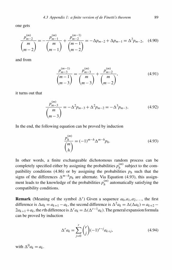
4.3 Appendix 1: a finite version of de Finetti’s theorem 89
one gets
p(m)m−2(m
m − 2
) = − p(m)m−1(m
m − 1
) + p(m−1)m−2(
m − 1
m − 2
) = − pm−2 + pm−1 = 2pm−2, (4.90)
and from
p(m−1)m−3(
m − 1
m − 3
) = p(m)m−3(m
m − 3
) + p(m)m−2(m
m − 2
) , (4.91)
it turns out that
p(m)m−3(m
m − 3
) = − 2pm−3 + 2pm−2 = − 3pm−3. (4.92)
In the end, the following equation can be proved by induction
p(m)h(m
h
) = (−1)m−h m−hph. (4.93)
In other words, a finite exchangeable dichotomous random process can becompletely specified either by assigning the probabilities p(m)
h subject to the com-patibility conditions (4.86) or by assigning the probabilities ph such that thesigns of the differences m−hph are alternate. Via Equation (4.93), this assign-ment leads to the knowledge of the probabilities p(m)
h automatically satisfying thecompatibility conditions.
Remark (Meaning of the symbol r) Given a sequence a0,a1,a2, . . ., the firstdifference is ak = ak+1 −ak , the second difference is 2ak = ( ak) = ak+2 −2ak+1+ak , the rth difference is rak = ( r−1ak).The general expansion formulacan be proved by induction
rak =r∑
j=0
(r
j
)(−1)r−jak+j, (4.94)
with 0ak = ak .
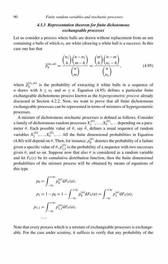
90 Finite random variables and stochastic processes
4.3.3 Representation theorem for finite dichotomousexchangeable processes
Let us consider a process where balls are drawn without replacement from an urncontaining n balls of which n1 are white (drawing a white ball is a success). In thiscase one has that
p(n1,m)h =
(n1
h
)(n − n1
m − h
)(
n
m
) =
(m
h
)(n − m
n1 − h
)(
n
n1
) , (4.95)
where p(n1,m)h is the probability of extracting h white balls in a sequence of
n draws with h ≤ n1 and m ≤ n. Equation (4.95) defines a particular finiteexchangeable dichotomous process known as the hypergeometric process alreadydiscussed in Section 4.2.2. Now, we want to prove that all finite dichotomousexchangeable processes can be represented in terms of mixtures of hypergeometricprocesses.
A mixture of dichotomous stochastic processes is defined as follows. Considera family of dichotomous random processes X (θ)
1 , . . . ,X (θ)n , . . . depending on a para-
meter θ . Each possible value of θ , say θ , defines a usual sequence of random
variables X (θ)1 , . . . ,X (θ)
n , . . .. All the finite dimensional probabilities in Equation
(4.80) will depend on θ . Then, for instance, p(θ)0 denotes the probability of a failure
given a specific value of θ , p(θ)1,1 is the probability of a sequence with two successes
given θ , and so on. Suppose now that also θ is considered as a random variableand let Fθ (x) be its cumulative distribution function, then the finite dimensionalprobabilities of the mixture process will be obtained by means of equations ofthis type
p0 =∫ +∞
−∞p(u)
0 dFθ (u),
p1 = 1 − p0 = 1 −∫ +∞
−∞p(u)
0 dFθ (u) =∫ +∞
−∞p(u)
1 dFθ (u),
p1,1 =∫ +∞
−∞p(u)
1,1dFθ (u),
. . . .
Note that every process which is a mixture of exchangeable processes is exchange-able. For the case under scrutiny, it suffices to verify that any probability of the
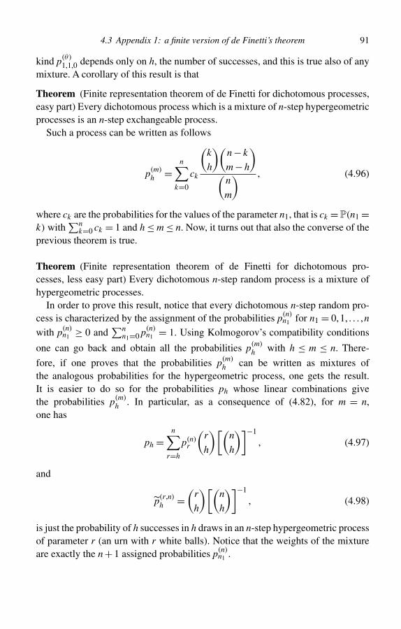
4.3 Appendix 1: a finite version of de Finetti’s theorem 91
kind p(θ)1,1,0 depends only on h, the number of successes, and this is true also of any
mixture. A corollary of this result is that
Theorem (Finite representation theorem of de Finetti for dichotomous processes,easy part) Every dichotomous process which is a mixture of n-step hypergeometricprocesses is an n-step exchangeable process.
Such a process can be written as follows
p(m)h =
n∑k=0
ck
(k
h
)(n − k
m − h
)(
n
m
) , (4.96)
where ck are the probabilities for the values of the parameter n1, that is ck = P(n1 =k) with
∑nk=0 ck = 1 and h ≤ m ≤ n. Now, it turns out that also the converse of the
previous theorem is true.
Theorem (Finite representation theorem of de Finetti for dichotomous pro-cesses, less easy part) Every dichotomous n-step random process is a mixture ofhypergeometric processes.
In order to prove this result, notice that every dichotomous n-step random pro-cess is characterized by the assignment of the probabilities p(n)
n1 for n1 = 0,1, . . . ,n
with p(n)n1 ≥ 0 and
∑nn1=0 p(n)
n1 = 1. Using Kolmogorov’s compatibility conditions
one can go back and obtain all the probabilities p(m)h with h ≤ m ≤ n. There-
fore, if one proves that the probabilities p(m)h can be written as mixtures of
the analogous probabilities for the hypergeometric process, one gets the result.It is easier to do so for the probabilities ph whose linear combinations givethe probabilities p(m)
h . In particular, as a consequence of (4.82), for m = n,one has
ph =n∑
r=h
p(n)r
(r
h
)[(n
h
)]−1
, (4.97)
and
p(r,n)h =
(r
h
)[(n
h
)]−1
, (4.98)
is just the probability of h successes in h draws in an n-step hypergeometric processof parameter r (an urn with r white balls). Notice that the weights of the mixtureare exactly the n + 1 assigned probabilities p(n)
n1 .
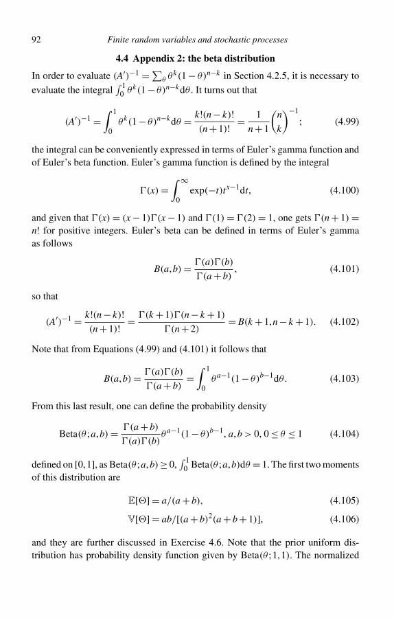
92 Finite random variables and stochastic processes
4.4 Appendix 2: the beta distribution
In order to evaluate (A′)−1 =∑θ θk(1 − θ)n−k in Section 4.2.5, it is necessary to
evaluate the integral∫ 1
0 θk(1 − θ)n−kdθ . It turns out that
(A′)−1 =∫ 1
0θk(1 − θ)n−kdθ = k!(n − k)!
(n + 1)! = 1
n + 1
(n
k
)−1
; (4.99)
the integral can be conveniently expressed in terms of Euler’s gamma function andof Euler’s beta function. Euler’s gamma function is defined by the integral
�(x) =∫ ∞
0exp(−t)tx−1dt, (4.100)
and given that �(x) = (x − 1)�(x − 1) and �(1) = �(2) = 1, one gets �(n + 1) =n! for positive integers. Euler’s beta can be defined in terms of Euler’s gammaas follows
B(a,b) = �(a)�(b)
�(a + b), (4.101)
so that
(A′)−1 = k!(n − k)!(n + 1)! = �(k + 1)�(n − k + 1)
�(n + 2)= B(k + 1,n − k + 1). (4.102)
Note that from Equations (4.99) and (4.101) it follows that
B(a,b) = �(a)�(b)
�(a + b)=∫ 1
0θa−1(1 − θ)b−1dθ . (4.103)
From this last result, one can define the probability density
Beta(θ ;a,b) = �(a + b)
�(a)�(b)θa−1(1 − θ)b−1, a,b > 0, 0 ≤ θ ≤ 1 (4.104)
defined on [0,1], as Beta(θ ;a,b) ≥ 0,∫ 1
0 Beta(θ ;a,b)dθ = 1. The first two momentsof this distribution are
E[�] = a/(a + b), (4.105)
V[�] = ab/[(a + b)2(a + b + 1)], (4.106)
and they are further discussed in Exercise 4.6. Note that the prior uniform dis-tribution has probability density function given by Beta(θ ;1,1). The normalized
4.6 Summary 93
posterior distribution is characterized by the probability density function
p(θ |k,n) = (n + 1)
(n
k
)θk(1 − θ)n−k = �(n + 2)
�(k + 1)�(n − k + 1)θk(1 − θ)n−k ,
(4.107)
which is nothing other than Beta(θ ;k + 1,n − k + 1). Finally, recalling thatP(Xn+1 = 1|X(n)(k)) = ∑
θ θ · P(� = θ |X(n)(k)) = Eposterior(�), from (4.105),one immediately gets Laplace’s succession rule:
P(Xn+1 = 1|X(n)(k)) = k + 1
n + 2. (4.108)
4.5 Exercises
4.1 Prove that the inverse image of all labels divides the set � into equivalenceclasses.
4.2 Prove that E(a + bX ) = a + bE(X ).4.3 Prove that:
1. V(X ) = E(X 2)−E2(X );2. V(X + a) = V(X );3. V(bX ) = b2V(X ).
4.4 Prove the properties of the indicator function (see Section 4.1.8).4.5 Apply the total probability theorem to P(X2 = x2|X1 = x1), considering that
they are two results of draws from a bivariate urn of indefinite composition.4.6 Compute the expected value and the variance for the beta distribution.
4.6 Summary
Many results of Chapters 2 and 3 can be conveniently reformulated in the languageof random variables and stochastic processes. A random variable is a measurablefunction mapping a probability space into another probability space. A functionis another name for a categorization of objects. Therefore, it is natural to intro-duce random variables Xi whose range is a label set denoting the g categories intowhich n objects are divided. Random variables are characterized by their proba-bility distributions. For a numerical random variable, the distribution can often besummarized by two numbers: the expected value or mathematical expectation andthe variance. The mathematical expectation denotes a ‘typical’ value of the distri-bution, whereas the variance represents typical fluctuations of the random variablearound this typical value.
When two or more random variables on the same probability space are consid-ered, it is interesting to study their covariance, indicating how much these variables
94 Finite random variables and stochastic processes
are correlated. A random vector is characterized by a joint probability distribution.Sums of the joint probability distribution on the possible values of all but onerandom variable lead to the so-called marginal distribution.
Asequence of random variables is a stochastic process. The index of the sequenceoften denotes time, but this is not necessarily the case. In many examples of interest,the index set runs on the objects that are studied. Stochastic (or random) processesare characterized by the set of finite dimensional probability distributions (appro-priate joint distributions for the variables in the sequence) and these distributionsmust satisfy Kolmogorov’s compatibility conditions.
Among all stochastic processes, exchangeable processes are those for which theprobability of a sequence does not depend on the specific outcomes, but only onthe number of occurrences of any category. This greatly simplifies the analysis ofsuch processes. It turns out that finite exchangeable processes can be representedas mixtures of the hypergeometric process. The hypergeometric process has a verysimple urn model: drawing balls from an urn without replacement. For large samplesizes, this process coincides with sampling with replacement: the usual Bernoullianprocess. Both processes are instances of another important class of exchangeablestochastic processes: the family of Pólya processes. The analysis of these processesin terms of predictive laws leads to Laplace’s rule of succession – a milestone ofpredictive probabilistic inference.
Further reading
A.N. Kolmogorov and S.V. Fomin discuss the meaning of maps (or functions) ascategorizations at the beginning of their book on functional analysis.
A.N. Kolmogorov and S.V. Fomin, Elements of the Theory of Functions and FunctionalAnalysis, Dover, New York (1999).
The relevance quotient and its invariance are the subject of an essay byD. Costantini.
D. Costantini, The Relevance Quotient, Erkenntniss, 14, 149–157 (1979).
This issue is discussed in detail at the end of the next chapter.L. Brillouin used the concepts developed in this chapter to derive quantum
statistics. His paper was published in 1927.
L. Brillouin, Comparaison des différentes statistiques appliquées aux problèmes de quanta,Annales de Physique, Paris, VII: 315–331 (1927).
D. Costantini and U. Garibaldi noticed the analogy between the tools used byBrillouin and the tools used in probabilistic predictive inference.
References 95
D. Costantini and U. Garibaldi, Una formulazione probabilistica del Principio di esclusionedi Pauli nel contesto delle inferenze predittive, Statistica, anno LI, n.1, p. 21 (1991).
An account in English of these results is available:
D. Costantini and U. Garibaldi, The Ehrenfest Fleas: From Model to Theory, Synthese, 139(1), 107–142 (2004).
There are many good books on random variables and stochastic processes. Aclassical reference is the book by J.L. Doob.
J.L. Doob, Stochastic Processes (Wiley Classics Library), Wiley, New York (1990).
The introductory textbooks by S. Karlin and H.M. Taylor
S. Karlin and H.M. Taylor, A First Course in Stochastic Processes, Academic Press, London(1975).
and by S.M. Ross
S.M. Ross, Stochastic Processes, Wiley, New York (1983).
are also useful classical references. Cambridge University Press has just publisheda book on stochastic processes for physicists including some elements of modernprobability theory.
K. Jacobs, Stochastic Processes for Physicists, Cambridge University Press, Cambridge,UK (2009).
The proof in Section 4.3 is adapted from
L. Daboni and A. Wedlin, Statistica. Un’introduzione all’impostazione neo-bayesiana,UTET, Turin (1982).
a book on neo-Bayesian statistics.
References
[1] J.S. Mill, On the Definition of Political Economy and the Method of Investigation Properto It, essay 5 in J.S. Mill, Essays on Some Unsettled Questions of Political Economy,John W. Parker, West Strand, London (1844).
[2] P.-R. de Montmort, Essay d’analyse sur les jeux d’hazard, J. Quillau, Paris (1708).Reprinted by the American Mathematical Society in 2006.
5
The Pólya process
The multivariate generalized Pólya distribution plays a key role in the finitaryanalysis of many interesting problems. It gives the distribution of the statisticaldescriptions for the so-called Pólya stochastic process. As discussed in Chapter 4,such a process has a simple urn model interpretation. Therefore, this chapter isdevoted to a detailed analysis of the generalized multivariate Pólya distributionand of the related stochastic process.
After studying this chapter you should be able to:
• define the Pólya process;• derive the multivariate generalized Pólya distribution as the sampling distribution
of the Pólya process;• compute the expected value and the variance of the multivariate generalized
Pólya distribution;• discuss some remarkable limits of the multivariate generalized Pólya distribution;• marginalize the multivariate generalized Pólya distribution;• characterize the Pólya process in terms of the invariance of the heterorelevance
coefficient.
5.1 Definition of the Pólya process
The sequence X1,X2, . . . ,Xn, with Xi ∈ {1, . . . ,g}, is a generalized Pólya process ifthe predictive probability of the process is given by (4.72), rewritten below for thesake of clarity
P(Xm+1 = j|X1 = x1, . . . ,Xm = xm) = αj + mj
α + m, (5.1)
where mj = #{Xi = j, i = 1, . . . ,m} is the number of occurrences of the jth category inthe evidence (X1 = x1, . . . ,Xm = xm), and m is the number of observations or trials.As for the parameters α and αj, in the usual Pólya process, αj is a positive integer,representing the number of balls of type (colour) j in the auxiliary Pólya urn; α is the
96
5.1 Definition of the Pólya process 97
total number of balls in the urn and it is given by α =∑gj=1 αj. If αj is positive but
real, it can be interpreted as the initial weight of the jth category, it being understoodthat the prize (the added weight) of the drawn category is always just 1. The meaningof αj becomes clearer if one defines pj = αj/α, then Equation (5.1) can be written
P(Xm+1 = j|X1 = x1, . . . ,Xm = xm) = αpj + mj
α + m= α
α + mpj + m
α + m
mj
m, (5.2)
and pj has a natural interpretation as prior (or initial) probability for the jth category:pj = αj/α = P(X1 = j). Note that in this way, the limit α → ∞ has an immediateinterpretation as (5.2) becomes
P(Xm+1 = j|X1 = x1, . . . ,Xm = xm) = pj, (5.3)
leading to the i.i.d. multinomial distribution. In other words, the distribution ofthe generalized Pólya process converges to the distribution of the multinomialprocess when the parameter α diverges. When αj is negative, if |αj| is integer andmj ≤ |αj| = |α|pj, Equation (5.1) still represents a probability and it can be written as
P(Xm+1 = j|X1 = x1, . . . ,Xm = xm) = |α|pj − mj
|α|− m, (5.4)
but here, the number of variables (observations or trials) is limited by |α|. Asdiscussed in Section 4.2.2, Equation (5.4) leads to the hypergeometric distribution.Therefore, in the following, the general case (5.1) will be studied, with the totalweight α belonging to the set α ∈ (0,∞) ∪ {−n,−n − 1,−n − 2, . . . ,−∞}, whichis the union of the generalized Pólya and the hypergeometric domain, with themultinomial case appearing as both α → −∞ and α → +∞.
5.1.1 The finite dimensional distributions
As discussed in Section 4.2, Equation (4.50) shows that a knowledge of predic-tive probabilities leads to knowledge of the finite dimensional distributions P(X1 =x1, . . . ,Xn = xn). In the specific case under scrutiny, it suffices to consider the funda-mental sequence X(m)
f = (1, . . . ,1, . . . ,g, . . . ,g), consisting of m1 labels 1 followedby m2 labels 2, and so on, ending with mg occurrences of label g. As a direct con-sequence of Equations (4.50) and (5.1), the probability of this sequence is given by
α1
α
α1 + 1
α + 1. . .
α1 + m1 − 1
α + m1 − 1
α2
α + m1
α2 + 1
α + m1 + 1. . .
α2 + m2 − 1
α + m1 + m2 − 1. . .
. . .αg
α + m1 + m2 + . . .+ mg−1
αg + 1
α + m1 + m2 + . . .+ mg−1 + 1. . .
. . .αg + mg − 1
α + m1 + m2 + . . .+ mg − 1= α
[m1]1 · · ·α[mg ]
g
α[m] . (5.5)
98 The Pólya process
Recalling that m1 + m2 + . . . + mg = m, the previous formula can be re-writtenin a more compact way, in terms of rising factorials. Note that this result doesnot depend on the order of appearance of the categories. Indeed, the probabilityof a different sequence with the same values of m = (m1, . . . ,mg) would have thesame denominator and identical (but permuted) terms in the numerator. This meansthat the Pólya process is exchangeable and that the finite dimensional distributionsdepend only on the frequency vector m. The finite dimensional distribution is
P(X(m)) = 1
α[m]g∏
i=1
α[mi]i . (5.6)
So the predictive probability (5.1) yields the law (5.6); it turns out that the converseis also true, as from the definition of conditional probability
P(Xm+1 = j|X(m)) = P(X(m),Xm+1 = j)
P(X(m))= αj + mj
α + m, (5.7)
where X(m) is an evidence with frequency vector m = (m1, . . . ,mg), both the numer-ator and the denominator follow (5.6), and the calculation is left to the reader as auseful exercise on Pochhammer symbols.
The sampling distribution is the probability of the frequency vector m. In orderto evaluate it as a function of the size m, it is sufficient to multiply (5.6) by thenumber of distinct equiprobable sequences leading to m
P(m) = Polya(m;α) = m!∏gi=1 mi!
∏gi=1 α
[mi]i
α[m] = m!α[m]
g∏i=1
α[mi]i
mi! ; (5.8)
this equation defines the Pólya distribution which has already been informallydiscussed in Section 4.2.2.
5.1.2 Example: the dichotomous generalized Pólya distribution and its limits
The dichotomous (or bivariate) case, g = 2, is sufficient to illustrate all the essentialproperties of the Pólya process. Let Xi = 0,1, and define (m1 = h,m0 = m − h) asthe frequency vector of X1, . . . ,Xm. Then h = #{Xi = 1} is the number of observedsuccesses and Sm = h is a random variable whose values h vary according toh ∈ {0,1, . . . ,m}. Moreover, one can write Sm =∑m
i=1 Xi. In this simple case themultivariate distribution (5.8) simplifies to
P(Sm = h) = m!m0!m1!
α[m0]0 α
[m1]1
α[m] =(
m
h
)α
[h]1 α
[m−h]0
α[m] . (5.9)
5.1 Definition of the Pólya process 99
The sampling distribution of the dichotomous Pólya process is also known as thebeta-binomial distribution. The following remarks are noteworthy.
1. (Uniform distribution) One has 1[n] = n! and 2[n] = (n+1)!; if α0 = α1 = 1, thenα = α0 +α1 = 2, and it turns out that
P(Sm = h) = m!h!(m − h)!
h!(m − h)!(m + 1)! = 1
m + 1; (5.10)
this is the uniform distribution on all frequency vectors of m elements and g = 2categories.
2. (Binomial distribution) For x � n, one has x[n] = x(x + 1) . . . (x + n − 1) xn;moreover, one can set α0 = αp0, and α1 = αp1. Therefore, one obtains that
limα→∞P(Sm = h)
= limα→∞
(m
h
)αh
1αm−h0
αm=(
m
h
)ph
1(1 − p1)m−h; (5.11)
this is the binomial distribution of parameters m and p1. In other words, if theinitial urn has a very large number of balls, the Pólya prize is inessential tocalculate the predictive probability, they are all equal for each category andthe Pólya process cannot be distinguished from repeated Bernoullian trials, asalready discussed above.
3. (Hypergeometric distribution) Given that x[n] = x(x + 1) . . . (x + n − 1), if x isnegative, and n ≤ |x|, one gets x[n] = (−1)n|x|(|x|−1) . . . (|x|−n+1), meaningthat x[n] = (−1)n |x|[n], where x[n] = x(x−1) . . . (x−n+1) is the so-called falling(or lower) factorial, and setting α1 = −N1 = −Np1, α0 = −N0 = −Np0, withp1 + p0 = 1, one gets:
P(Sm = h) = m!h!(m − h)!× (−1)hN1 · · ·(N1 − h + 1)(−1)m−hN0 · · ·(N1 − n + h + 1)
(−1)mN · · ·(N − m + 1),
(5.12)
leading to the hypergeometric distribution
P(Sm = h) =
(N1
h
)(N0
m − h
)(
N
m
) =(
m
h
)(N − m
N1 − h
)(
N
N1
) , (5.13)
100 The Pólya process
which is the usual sampling distribution from a hypergeometric urn with N0,N1
balls and N = N1 + N0.4. (Limit of the hypergeometric distribution) Also for the falling factorial x � n
yields x[n] xn. Therefore, one obtains
limα→−∞P(Sm = h) =
(m
h
)ph
1(1 − p1)m−h; (5.14)
in other words, sampling without replacement from a very large urn cannot bedistinguished from sampling with replacement.
5.2 The first moments of the Pólya distribution
Consider the evidence vector X(m) = (X1 = x1, . . . ,Xm = xm). In the dichotomouscase, h = #{Xi = 1} can also be written as Sm = h =∑m
i=1 Xi. In order to gener-alize this definition to the general case of g categories, it is natural to introducethe indicator function IXi=j(ω) = I (j)
i , and define S(j)m =∑m
i=1 I (j)i . Therefore, the
random variable S(j)m gives the number of successes for the jth category out of m
observations or trials and S(j)m = mj. The expected value and the variance for S(j)
m canbe computed with the help of two simple theorems, which will be further discussedin Exercise 5.1 and Exercise 5.2.
Theorem (Expected value for the sum of m random variables) One has
E
(m∑
i=1
Xi
)=
m∑i=1
E(Xi). (5.15)
This theorem will be proven in Exercise 5.1.
Theorem (Variance of the sum of m random variables)
V
(m∑
i=1
Xi
)=
m∑i=1
V(Xi)+ 2m∑
i=1
m∑j=i+1
C(Xi,Xj). (5.16)
The proof of this theorem will be presented in Exercise 5.2.
One has to determine E(I (k)i ) and E(I (k)
i I (k)j ). As for the expected value, one
has that E(I (k)i ) = 1 · P(I (k)
i = 1) + 0 · P(I (k)i = 0) = P(I (k)
i = 1) coinciding withthe marginal probability of success, that is of observing category k at the ith step.From Equation (5.7), in the absence of any evidence, one has P(I (k)
i = 1) = P(Xi =k) = αk/α = pk . Therefore, the random variables I (k)
i are equidistributed (they are
5.2 The first moments of the Pólya distribution 101
exchangeable), and E(S(k)m ) =∑m
i=1 E(I (k)i ) = mE(I (k)
1 ), yielding
E(S(k)m ) = mpk . (5.17)
Considering the variance V(S(k)m ), as a consequence of Equation (5.16), the covari-
ance matrix of I (k)1 , . . . , I (k)
m is needed. Due to the equidistribution of I (k)1 , . . . , I (k)
m , the
moment E[(I (k)i )2] is the same for all i, and because of exchangeability E(I (k)
i I (k)j )
is the same for all i, j, with i �= j. Note that (I (k)i )2 = I (k)
i and this means that
E[(I (k)i )2] = pk ; it follows that
V(I (k)i ) = E[(I (k)
i )2]−E2(I (k)i ) = pk − p2
k = pk(1 − pk). (5.18)
In Exercise 5.3, it is shown that
E(I (k)i I (k)
j ) = P(Xi = k,Xj = k); (5.19)
now, from exchangeability, from (5.19) and from (5.7), one gets
E(I (k)i I (k)
j ) = P(Xi = k,Xj = k) = P(X1 = k,X2 = k)
= E(I (k)1 I (k)
2 ) = P(X1 = k)P(X2 = k|X1 = k) = pkαk + 1
α + 1. (5.20)
Therefore, the covariance matrix is given by
C(I (k)i , I (k)
j ) = C(I (k)1 , I (k)
2 )
= E(I (k)1 I (k)
2 )−E(I (k)1 )E(I (k)
2 ) = pk(1 − pk)
α + 1. (5.21)
From this equation and from Equation (5.18), it follows that the correlationcoefficient is given by
ρ(I (k)1 , I (k)
2 ) = 1
α + 1; (5.22)
therefore, if α → 0, the correlation coefficient converges to 1, whereas if α → ±∞,the correlation coefficient vanishes. The variance of the sum S(k)
m follows fromEquations (5.16), (5.18) and (5.21)
V(S(k)m ) = mV(I (k)
1 )+ m(m − 1)C(I (k)1 , I (k)
2 ) = mpk(1 − pk)α + m
α + 1. (5.23)
5.2.1 Remarks on the first moments; the coefficient of variation andlack of self-averaging
In the previous derivation, the initial probability pk and the ratio αk/α wereused indifferently for computational convenience. Regarding the analysis of the
102 The Pólya process
moments, it is useful to consider pk and α as independent parameters. One can seethat the expected value of successes only depends on pk , the probability of the cat-egory, and not on the total weight α; on the contrary, the variance strongly dependson α; Moreover, one has that:
1. if α → ∞, V∞(S(k)m ) = mpk(1 − pk), recovering the variance of the binomial
distribution, as expected;
2. if 0 < α < ∞, a factorα + m
α + 1multiplies V∞(S(k)
m ) and this factor is O(m) for
large m;3. if α < 0, with |α| ≥ m, a factor (|α| − m)/(|α| − 1) multiplies V∞(S(k)
m ); thisfactor is a decreasing function of m, and it vanishes for m = |α|. This is expectedin sampling without replacement from an urn containing |α| balls.
In the binomial case (|α| → ∞), the relative frequency of successes, given byS(k)
m /m, has expected value E∞(S(k)m /m) = E∞(S(k)
m )/m = pk , whereas its varianceis V∞(S(k)
m /m) = V∞(S(k)m )/m2 = pk(1 − pk)/m. The coefficient of variation of a
positive random variable is defined as
CVX = σX
E(X ), (5.24)
where σX = √V(X ) is the standard deviation of X , and CVX is a dimensionless
number, expressing the relative deviation with respect to the expected value. Forthe random variable S(k)
m /m, in the case |α| → ∞, one has
CVS(k)
m /m=
σS(k)
m /m
E(S(k)m /m)
≈ 1√m
√α −αk
αk, (5.25)
yielding a vanishing relative deviation as m increases. Therefore, the sequence isself-averaging, meaning that expected relative fluctuations vanish as m increases,so that the behaviour of the sequence becomes closer and closer to the deterministiccase. However, in the general case 0 < α < ∞, one gets
CVS(k)
m /m= 1√
m
√α −αk
αk
α + m
α + 1. (5.26)
Therefore, one finds that the coefficient of variation does not vanish in the limitm → ∞:
limm→∞CV
S(k)m /m
=√
α −αk
αk
1
α + 1. (5.27)
In other words, the behaviour is fully probabilistic also in the limit m → ∞. Notethat the case α < 0 is not interesting, as after m = |α| steps the process ends andCV
S(k)m /m
= 0 for m = |α|.
5.2 The first moments of the Pólya distribution 103
5.2.2 Again on Ehrenfest and Boltzmann
Returning to the examples of Chapter 3, if n molecules independently and symmet-rically partition into g = 2 categories (two symmetrical parts of a box) labelled as0,1, the predictive probability becomes
P(Xm+1 = j|X1 = x1, . . . ,Xm = xm) = pj = 1
2, (5.28)
where j = 0,1. This predictive probability leads to the limit of the generalized Pólyadistribution for αj → ∞, α → ∞ and pj = αj/α = 1/2. Let Sm = km describe thenumber of elements in category 1. One has
E(Sn) = np1 = n/2, (5.29)
and
V(Sn) = np1(1 − p1) = n/4, (5.30)
and Equation (5.26) eventually leads to
CVSn/n = σSn/n
E(Sn/n)= 1√
n. (5.31)
For a gas in normal conditions occupying a volume of 1 cm3, the number ofmolecules is n ≈ 1020; therefore CVSn/n ≈ 10−10, or one over 10 USA billions.Without entering the exact calculation, one could bet some billions against 1 that thefraction of molecules in side 1 is 0.5±10−10. In this simple case the expected valuesummarizes the whole phenomenon, and probability leads to the same conclusionas a deterministic reasoning, claiming that particles are 50 : 50-distributed.
On the contrary, in the case of n energy elements to be divided into g = 2molecules, in Section 3.4.3, it was assumed that they follow a uniform generalizedPólya distribution with α1 = α2 = 1 (indeed, this is how the result of Section 3.4.3can be re-interpreted now). In this case one has again that E(Sn) = n/2, but now
V(Sn) = n
4
2 + n
2 + 1= n(n + 2)
12. (5.32)
The variance of the relative frequency is
V(Sn/n) = n(n + 2)
12n2≈ 1/12, (5.33)
and
σSn/n ≈ 1
2
√1
3. (5.34)
104 The Pólya process
There is no self-averaging, as CVSn/n ≈ √1/3. In this case, the distribution of Sn is
uniform on the n + 1 values 0,1, . . . ,n, and the distribution of Sn/n is uniform on0,1/n, . . . ,1. It is always true that the expected value of Sn/n is 1/2, but this doesnot summarize the phenomenon at all. If one were to bet on a value, one should putthe same odds 1 : n on each of the n + 1 numbers 0,1, . . . ,n.
5.3 Label mixing and marginal distributions
5.3.1 Label mixing
The g-variate generalized Pólya distribution has a nice property which is useful forlabel mixing as defined by R. von Mises. Starting from (5.1), how can P(Xm+1 ∈A|X1 = x1, . . . ,Xm = xm) be obtained, where the set A is a set of categories A ={j1, . . . , jr}? The answer to this question is not difficult: it turns out that
P(Xm+1 ∈ A|X(m)) =r∑
i=1
P(Xm+1 = ji|X(m)), (5.35)
where, as usual, X(m) = (X1 = x1, . . . ,Xm = xm) summarizes the evidence. In thePólya case, P(Xm+1 = j|X(m)) is a linear function of both the weights and theoccupation numbers; therefore one gets
P(Xm+1 ∈ A|X(m)) =
∑j∈A
αj +∑j∈A
mj
α + m= αA + mA
α + m, (5.36)
where αA =∑j∈A αj and mA =∑j∈A mj. As a direct consequence of (5.36), themarginal distributions of the g-variate generalized Pólya distribution are givenby the dichotomous Pólya distribution of weights αi and α − αi, where i is thecategory with respect to which the marginalization is performed. In other words,one finds that ∑
mj , j �=i
Polya(m;α) = Polya(mi,m − mi;αi,α −αi). (5.37)
5.3.2 The geometric distribution as a marginal distribution of the uniformmultivariate Pólya distribution
Consider a g-variate generalized Pólya distribution with parameters αi = 1,i = 1, . . . ,g and α = g. Its predictive probability is
P(Xm+1 = j|X1 = x1, . . . ,Xm = xm) = 1 + mj
g + m, (5.38)
5.3 Label mixing and marginal distributions 105
and the sampling distribution after n steps is
P(n) = n!α[n]
g∏i=1
α[ni]i
ni! = n!g[n] = n!(g − 1)!
(n + g − 1)! =(
n + g − 1
n
)−1
, (5.39)
where the fact that 1[x] = x! was used. In the usual Boltzmann’s example, one isin the presence of n energy elements accommodating on g molecules so that anyconfiguration of molecules has the same probability. When the focus is on a singlemolecule, say the one numbered 1, all the other g −1 molecules can be consideredas a thermostat. What is the probability that n1 = k, meaning that the first moleculereceives k energy elements (and the thermostat receives n − k energy elements)?This is given by the marginalization of the uniform multivariate Pólya distribution,leading to
P(k) =(
n
k
)1[k](g − 1)[n−k]
g[n]
= n!g[n]
(g − 1)[n−k]
(n − k)! =
(n − k + (g − 1)− 1
n
)(
n + g − 1
n
) . (5.40)
In other words, all molecule descriptions being equiprobable, the number of descrip-tions assigning k energy elements to the chosen molecule coincides with thenumber of descriptions of n−k elements on the g −1 molecules of the thermostat.Equation (5.40) has an interesting limit for n,g � 1 with χ = n/g constant. First,one has that
(g − 1)[n−k]
g[n] = (g − 1)g(g + 1) · · ·(g + n − k − 2)
g(g + 1) · · ·(g + n − 1)
= (g − 1)
(g + n − k − 1) · · ·(g + n − 1) (g − 1)
(g + n)k+1, (5.41)
whereas, in the same limit,
n!(n − k)! nk ; (5.42)
therefore, combining the two previous equations leads to
P(k) gnk
(g + n)k+1= g
g + n
(n
g + n
)k
. (5.43)
106 The Pólya process
The meaning of χ = n/g is the average number of elements for each molecule; inthe limit, one is led to the geometric distribution of parameter χ
P(k) Geo(k;χ) = 1
1 +χ
(χ
1 +χ
)k
, (5.44)
where k can now vary from 0 to ∞. This is no longer a finite distribution, but still adiscrete distribution. This sort of limit, where n,g → ∞ and n/g = χ stays constantis often called thermodynamic limit by physicists.
The geometric distribution is often introduced in terms of the distribution for the(discrete) time of occurrence for the first success in a binomial process of parameterp = 1/(1 +χ), in which case one has
P(X = h) = p(1 − p)h−1, h = 1,2, . . . (5.45)
The alternative definition (5.44) describes the distribution of the waiting time of(the number of failures before) the first success; in the latter case
P(Y = k) = p(1 − p)k , k = 0,1,2, . . . (5.46)
The two definitions are connected by the transformation of random variablesY = X − 1.
5.3.3 The negative binomial distribution as a marginal distribution of thegeneral multivariate Pólya distribution
In the general case, the chosen category has weight α1 and the thermostat’s weightis α −α1; therefore the term α
[k]1 /k! does not simplify, g −1 is replaced by α −α1,
and the thermodynamic limit becomes n,α � 1 with χ = n/α. Considering thatx[m] = �(x + m)/�(x), one has
(α −α1)[n−k]
α[n] = �(α −α1 + n − k)
�(α −α1)
�(α)
�(α + n)
= �(α + n −α1 − k)
�(α + n)
�(α)
�(α −α1). (5.47)
In the limit x � m, �(x − m)/�(x) x−m. Therefore one finds
(α −α1)[n−k]
α[n] = αα1
(α + n)α1+k; (5.48)
5.3 Label mixing and marginal distributions 107
and, multiplying by n!/(n − k)! nk one finally has
P(k) NegBin(k;α1,χ)
= α[k]1
k!(
1
1 +χ
)α1(
χ
1 +χ
)k
, k = 0,1,2, . . . ; (5.49)
this distribution is called the negative binomial distribution; the geometric distri-bution (5.44) is a particular case in which α1 = 1 and α = g of (5.49). If α1 isan integer, the usual interpretation of the negative binomial random variable is thedescription of the (discrete) waiting time of (i.e. the number of failures before)the first α1th success in a binomial process with parameter p = 1/(1 + χ). Themoments of the negative binomial distribution can be obtained from the correspond-ing moments of the Polya(n1,n−n1;α1,α−α1) in the limit n,α � 1, with χ = n/α
yielding
E(n1 = k) = nα1
α→ α1χ , (5.50)
V(n1 = k) = nα1
α
α −α1
α
α + n
α + 1→ α1χ(1 +χ). (5.51)
Note that if α1 is an integer, k can be interpreted as the sum of α1 independent andidentically distributed geometric variables (and the expected value and the variancesimply sum).
If one considers two categories against the thermostat, one finds that the twocategories are described by two independent negative binomial distributions. Inother words, originally, the two categories were negatively correlated due to theconstraint
∑gi=1 ni = n. If the limit n → ∞ is considered, the thermostat removes
this entanglement, and the two occupation numbers become independent. Indeed,starting from
P(n1,n2,n − n1 − n2;α) = α[n1]1
n1!α
[n2]2
n2!(α −α1 −α2)
[n−n1−n2]
(n − n1 − n2)!n!
α[n] , (5.52)
in the limit n,α � 1, and χ = n/α, the first two terms do not change, while thelast term can be dealt with as before, replacing k by n1 + n2, and α1 by α1 + α2.Therefore, one gets
P(n1,n2;α1,α2,χ) = α[n1]1
n1!α
[n2]2
n2!(
1
1 +χ
)α1+α2(
χ
1 +χ
)n1+n2
= NegBin(n1;α1,χ)NegBin(n2;α2,χ). (5.53)
108 The Pólya process
5.3.4 Example: coins and agents
Consider a system of:
1. n = 10 coins, distributed over g = 2 agents;2. n = 100 coins, distributed over g = 20 agents;3. n = 1000 coins, distributed over g = 200 agents.
Let the predictive law be
P(Xm+1 = j|X1 = x1, . . . ,Xm = xm) = 1 + mj
g + m. (5.54)
For all the three cases described above, one has n/g = 5. How does the marginaldistribution for the first agent change? In the first case P1(n1 = k) is the uniformdichotomous Polya(n1,10 − n1;1,1); therefore, one has P1(n1 = k) = 1/11, k =0,1, . . . ,10, E1(n1) = 5 = n/g, and from Equation (5.23), one finds V1(n1) = 10.In the second case P2(n1 = k) is the marginal of the uniform 20-variate Pólya,that is Polya(n1,100 − n1;1,19); therefore E2(n1) = 5, but now V2(n1) = 27.1.Here the situation dramatically changes: the domain of the distribution enlargesfrom 0, . . . ,10 to 0, . . . ,100, but the expected value is always 5. The distributionis no longer uniform; it is rapidly decreasing. There is a probability equal to 0.13that n1 > 10. In the third case P3(n1 = k) = Polya(n1,1000 − n1;1,199), againE3(n1) = 5, but now V3(n1) = 29.7 and P(n1 > 100) = 5 ·10−9. If NegBin(k;1,5)
is used instead of Polya(n1,1000 − n1;1,199) one finds ENegBin(n1) = 5, andVNegBin(n1) = α1χ(1 + χ) = 30. Note that, usually, the negative binomial dis-tribution is parameterized by α1 and p = 1/(1 + χ); in the above case this meansα1 = 1,p = 1/6.
5.3.5 The Poisson distribution
In the case α →∞ andαi/α = pi for i = 1, . . . ,g, the g-variate generalized Pólya dis-tribution converges to the multinomial distribution, and its marginal is the binomialdistribution
P(k) = Bin(k;n,p1) =(
n
k
)pk
1(1 − p1)n−k , (5.55)
with p1 = α1/α (and focus, as usual, on the first category). In the symmetric caseone has pi = 1/g = p, from which one readily gets
P(k) = Bin (k;n,1/g) =(
n
k
)(1
g
)k (1 − 1
g
)n−k
. (5.56)
5.3 Label mixing and marginal distributions 109
In the thermodynamic limit n,g � 1, with λ = n/g, one also has p → 0, andn → ∞ while np = λ remains finite. Writing p = λ/n, one gets the so-called Poissondistribution
Bin(k;n,p) =(
n
k
)pk(1 − p)n−k nk
k!(
λ
n
)k (1 − λ
n
)n−k
→ λk
k! e−λ = Poi(k;λ). (5.57)
The moments of this distribution can be easily recovered from the moments of thebinomial:
EPoi(K) = limn→∞,p→0
np = λ, (5.58)
VPoi(K) = limn→∞,p→0
np(1 − p) = λ. (5.59)
These results can also be directly obtained from the definition in (5.57), but bymeans of rather cumbersome calculations.
In the above calculations, first the limit α → ∞ is performed, and then thethermodynamic limit. The converse is also possible, also leading to the Poissondistribution from the negative binomial distribution. From (5.49) one can see whathappens when α1 →∞, χ → 0 and the product α1χ =λ stays constant. The variouspieces of (5.49) behave as follows: α
[k]1 αk
1 , χ = n/α � 1, (1/(1 +χ))α1 (1 −χ)α1 = (1 −λ/α1)
α1 , (χ/(1 +χ))k χk , then one finally gets
NegBin(k;α1,χ) = α[k]1
k!(
1
1 +χ
)α1(
χ
1 +χ
)k
αk1
k!(
1 − λ
α1
)α1
χk (α1χ)k
k! e−α1χ
= λk
k! e−λ = Poi(k;λ). (5.60)
5.3.6 Binomial distribution as the thermodynamic limit of the g-variatehypergeometric distribution
The generalized g-variate Pólya distribution with negative integer weights coin-cides with the g-variate hypergeometric distribution; in this case, α1 and α − α1
are negative integers. Therefore α[k]1 = (−1)k(|α1|)(|α1| − 1) · · ·(|α1| − k + 1).
110 The Pólya process
Hence, the domain of n1 = k is limited, 0 ≤ k ≤ |α1|, with negative χ = n/α, and(5.49) becomes
(−1)k(|α1|
k
)(1
1 −|χ |)α1
( −|χ |1 −|χ |
)k
=(|α1|
k
)(1
1 −|χ |)−|α1|( |χ |
1 −|χ |)k
. (5.61)
Note that |χ | ≤ 1, as n ≤ |α|. For the sake of clarity, one can set |α1| = m, |χ | = p,and get (|α1|
k
)(1
1 −|χ |)−|α1|( |χ |
1 −|χ |)k
=(
m
k
)(1 − p)m pk
(1 − p)k
=(
m
k
)pk(1 − p)m−k = Bin(k;m,p). (5.62)
5.3.7 Example: random distribution of students into classrooms
Assume that in assigning students to classrooms in a high school, teachers initiallyhave n = 100 students to allocate, and they have to distribute them into g = 5classrooms; teachers choose an accommodation probability equal to
P(Xm+1 = j|X1 = x1, . . . ,Xm = xm) = 25 − mj
25 · 5 − m. (5.63)
This means that no classroom can contain more than 25 students, and each student,once called, has a uniform probability of ending up in one of the available places.The resulting generalized Pólya is a hypergeometric distribution with n = 100,g = 5, αi = −25, and α = −125. The expected number of students per classroomis n|αi|/α = 20, the variance is given by (5.23) leading to
V(n1) = 100 · 1
5· 4
5· 125 − 100
125 − 1= 3.2, (5.64)
with a standard deviation equal to σ = √3.2 = 1.8. Note that if the allocations were
independent, the variance would have been 100 · (1/5) ·4/5 = 16, and the standarddeviation σ = 4. From (5.13), the probability that a class (the first one, say, as theyare all equidistributed) receives k students is given by
P(k) =
(25
k
)(100
100 − k
)(
125
100
) . (5.65)
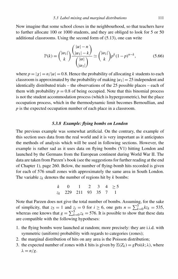
5.3 Label mixing and marginal distributions 111
Now imagine that some school closes in the neighbourhood, so that teachers haveto further allocate 100 or 1000 students, and they are obliged to look for 5 or 50additional classrooms. Using the second form of (5.13), one can write
P(k) =(|α1|
k
)( |α|− n
|α1|− k
)( |α|
|α1|)
(|α1|k
)pk(1 − p)n−k , (5.66)
where p = |χ | = n/|α| = 0.8. Hence the probability of allocating k students to eachclassroom is approximated by the probability of making |α1| = 25 independent andidentically distributed trials – the observations of the 25 possible places – each ofthem with probability p = 0.8 of being occupied. Note that this binomial processis not the student accommodation process (which is hypergeometric), but the placeoccupation process, which in the thermodynamic limit becomes Bernoullian, andp is the expected occupation number of each place in a classroom.
5.3.8 Example: flying bombs on London
The previous example was somewhat artificial. On the contrary, the example ofthis section uses data from the real world and it is very important as it anticipatesthe methods of analysis which will be used in following sections. However, theexample is rather sad as it uses data on flying bombs (V1) hitting London andlaunched by the Germans from the European continent during World War II. Thedata are taken from Parzen’s book (see the suggestions for further reading at the endof Chapter 1), page 260. Below, the number of flying-bomb hits recorded is givenfor each of 576 small zones with approximately the same area in South London.The variable zk denotes the number of regions hit by k bombs:
k 0 1 2 3 4 ≥ 5zk 229 211 93 35 7 1
Note that Parzen does not give the total number of bombs. Assuming, for the sakeof simplicity, that z5 = 1 and zi = 0 for i ≥ 6, one gets n = ∑5
k=0 kzk = 535,whereas one knows that g =∑5
k=0 zk = 576. It is possible to show that these dataare compatible with the following hypotheses:
1. the flying bombs were launched at random; more precisely: they are i.i.d. withsymmetric (uniform) probability with regards to categories (zones);
2. the marginal distribution of hits on any area is the Poisson distribution;3. the expected number of zones with k hits is given by E(Zk) = gPoi(k;λ), where
λ = n/g.
112 The Pólya process
Note that Xm = j means that the mth flying bomb hits the jth zone, and the hypothesisis made that
P(Xm+1 = j|X1 = x1, . . . ,Xm = xm) = 1
g. (5.67)
Then the sampling distribution on n = (n1, . . . ,ng) is the symmetric multinomialdistribution
P(n) = n!n1! · · ·ng !g
−n. (5.68)
Indeed, P(n) is exchangeable with respect to the g categories meaning that
P(n1 = k1, . . . ,ng = kg) = P(ni1 = k1, . . . ,nig = kg), (5.69)
where i1, . . . , ig is one of the g! permutations of 1, . . . ,g. Thus
P(n) =(
g!z0! · · ·zn!
)−1
P(z), (5.70)
where z = (z0,z1, . . . ,zn) is the frequency vector for n, or the partition vector forX(n). Equation (5.70) is analogous to Equation (4.59) for individual sequences andoccupation vectors. Note that for all vectors belonging to the same partition z,one has
g∏i=1
ni! =n∏
k=0
k!zk , (5.71)
as zk is the number of terms equal to k! appearing in∏g
i=1 ni!. Therefore, one getsthe following important equation
P(z) = g!∏ni=0 zi!P(n) = g!∏n
i=0 zi!n!∏g
k=1 nk !g−n = g!n!∏n
i=0 zi!(i!)zig−n, (5.72)
where n is any vector corresponding to z. The domain of P(z) is A = {z :∑535
k=0 zk =576,
∑535k=0 kzk = 535}; #A is large, but a closed analytical formula is not available.
Moreover, P(z) is an n + 1-dimensional distribution, not easily compared withempirical observations of z. There are two routes to derive numbers that can becompared with the available data:
1. calculation of E(Zk), an exact procedure if the marginal distribution is knownfor P(n);
2. an approximate search for the most probable vector, an approximate methodwhich can be traced back to Boltzmann.
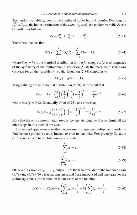
5.3 Label mixing and marginal distributions 113
The random variable Zk counts the number of zones hit by k bombs. Denoting byI (k)nj = Inj=k the indicator function of the event {nj = k}, the random variable Zk can
be written as follows
Zk = I (k)n1
+ I (k)n2
+ . . .+ I (k)ng
. (5.73)
Therefore, one has that
E(Zk) =g∑
j=1
E(I (k)nj
) =g∑
j=1
P(nj = k), (5.74)
where P(nj = k) is the marginal distribution for the jth category. As a consequenceof the symmetry of the multinomial distribution (5.68) the marginal distributionscoincide for all the variables ni, so that Equation (5.74) simplifies to
E(Zk) = gP(n1 = k). (5.75)
Marginalizing the multinomial distribution (5.68), it turns out that
P(n1 = k) =(
n
k
)(1
g
)k (1 − 1
g
)n−k
λk
k! e−λ, (5.76)
with λ = n/g = 0.93. Eventually, from (5.75), one arrives at
E(Zk) = g
(n
k
)(1
g
)k (1 − 1
g
)n−k
gλk
k! e−λ. (5.77)
Note that the only approximation used is the one yielding the Poisson limit; all theother steps in this method are exact.
The second approximate method makes use of Lagrange multipliers in order tofind the most probable vector. Indeed, one has to maximize P(z) given by Equation(5.72) and subject to the following constraints
n∑k=0
zk = g, (5.78)
n∑k=0
kzk = n. (5.79)
Of the n+1 variables z0, . . . ,zn, only n−1 of them are free, due to the two conditions(5.78) and (5.79). Two free parameters a and b are introduced and one searches thestationary values (the maximum in our case) of the function
L(z) = ln(P(z))+ a
(n∑
k=0
zk − g
)+ b
(n∑
k=0
kzk − n
), (5.80)
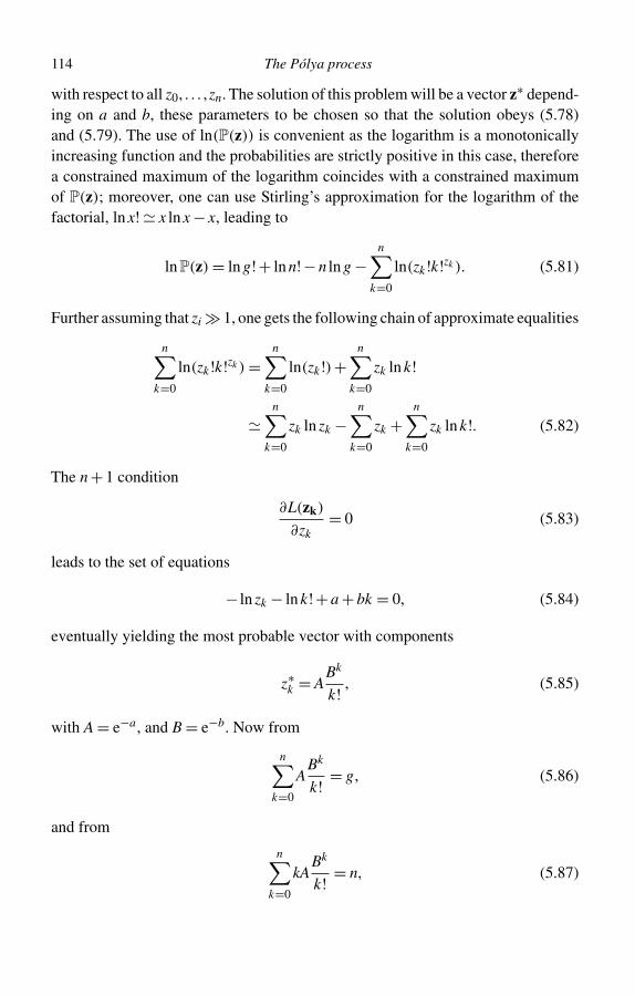
114 The Pólya process
with respect to all z0, . . . ,zn. The solution of this problem will be a vector z∗ depend-ing on a and b, these parameters to be chosen so that the solution obeys (5.78)and (5.79). The use of ln(P(z)) is convenient as the logarithm is a monotonicallyincreasing function and the probabilities are strictly positive in this case, thereforea constrained maximum of the logarithm coincides with a constrained maximumof P(z); moreover, one can use Stirling’s approximation for the logarithm of thefactorial, ln x! x ln x − x, leading to
lnP(z) = ln g!+ ln n!− n ln g −n∑
k=0
ln(zk !k!zk ). (5.81)
Further assuming that zi � 1, one gets the following chain of approximate equalities
n∑k=0
ln(zk !k!zk ) =n∑
k=0
ln(zk !)+n∑
k=0
zk ln k!
n∑
k=0
zk ln zk −n∑
k=0
zk +n∑
k=0
zk ln k!. (5.82)
The n + 1 condition
∂L(zk)
∂zk= 0 (5.83)
leads to the set of equations
− ln zk − ln k!+ a + bk = 0, (5.84)
eventually yielding the most probable vector with components
z∗k = A
Bk
k! , (5.85)
with A = e−a, and B = e−b. Now from
n∑k=0
ABk
k! = g, (5.86)
and from
n∑k=0
kABk
k! = n, (5.87)
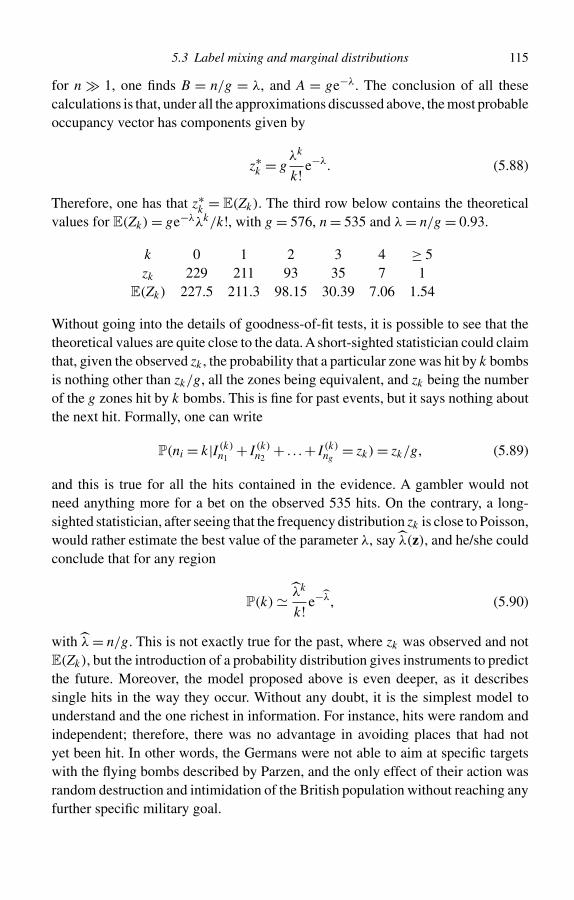
5.3 Label mixing and marginal distributions 115
for n � 1, one finds B = n/g = λ, and A = ge−λ. The conclusion of all thesecalculations is that, under all the approximations discussed above, the most probableoccupancy vector has components given by
z∗k = g
λk
k! e−λ. (5.88)
Therefore, one has that z∗k = E(Zk). The third row below contains the theoretical
values for E(Zk) = ge−λλk/k!, with g = 576, n = 535 and λ = n/g = 0.93.
k 0 1 2 3 4 ≥ 5zk 229 211 93 35 7 1
E(Zk) 227.5 211.3 98.15 30.39 7.06 1.54
Without going into the details of goodness-of-fit tests, it is possible to see that thetheoretical values are quite close to the data. A short-sighted statistician could claimthat, given the observed zk , the probability that a particular zone was hit by k bombsis nothing other than zk/g, all the zones being equivalent, and zk being the numberof the g zones hit by k bombs. This is fine for past events, but it says nothing aboutthe next hit. Formally, one can write
P(ni = k|I (k)n1
+ I (k)n2
+ . . .+ I (k)ng
= zk) = zk/g, (5.89)
and this is true for all the hits contained in the evidence. A gambler would notneed anything more for a bet on the observed 535 hits. On the contrary, a long-sighted statistician, after seeing that the frequency distribution zk is close to Poisson,would rather estimate the best value of the parameter λ, say λ(z), and he/she couldconclude that for any region
P(k) λk
k! e−λ, (5.90)
with λ = n/g. This is not exactly true for the past, where zk was observed and notE(Zk), but the introduction of a probability distribution gives instruments to predictthe future. Moreover, the model proposed above is even deeper, as it describessingle hits in the way they occur. Without any doubt, it is the simplest model tounderstand and the one richest in information. For instance, hits were random andindependent; therefore, there was no advantage in avoiding places that had notyet been hit. In other words, the Germans were not able to aim at specific targetswith the flying bombs described by Parzen, and the only effect of their action wasrandom destruction and intimidation of the British population without reaching anyfurther specific military goal.
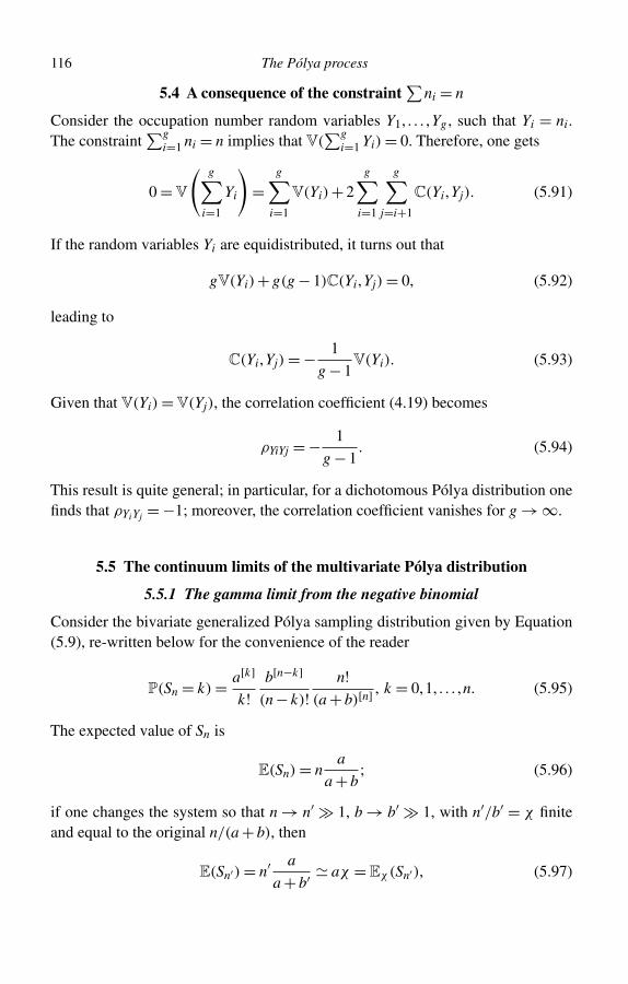
116 The Pólya process
5.4 A consequence of the constraint∑
ni = n
Consider the occupation number random variables Y1, . . . ,Yg , such that Yi = ni.The constraint
∑gi=1 ni = n implies that V(
∑gi=1 Yi) = 0. Therefore, one gets
0 = V
( g∑i=1
Yi
)=
g∑i=1
V(Yi)+ 2g∑
i=1
g∑j=i+1
C(Yi,Yj). (5.91)
If the random variables Yi are equidistributed, it turns out that
gV(Yi)+ g(g − 1)C(Yi,Yj) = 0, (5.92)
leading to
C(Yi,Yj) = − 1
g − 1V(Yi). (5.93)
Given that V(Yi) = V(Yj), the correlation coefficient (4.19) becomes
ρYiYj = − 1
g − 1. (5.94)
This result is quite general; in particular, for a dichotomous Pólya distribution onefinds that ρYiYj = −1; moreover, the correlation coefficient vanishes for g → ∞.
5.5 The continuum limits of the multivariate Pólya distribution
5.5.1 The gamma limit from the negative binomial
Consider the bivariate generalized Pólya sampling distribution given by Equation(5.9), re-written below for the convenience of the reader
P(Sn = k) = a[k]
k!b[n−k]
(n − k)!n!
(a + b)[n] , k = 0,1, . . . ,n. (5.95)
The expected value of Sn is
E(Sn) = na
a + b; (5.96)
if one changes the system so that n → n′ � 1, b → b′ � 1, with n′/b′ = χ finiteand equal to the original n/(a + b), then
E(Sn′) = n′ a
a + b′ aχ = Eχ(Sn′), (5.97)
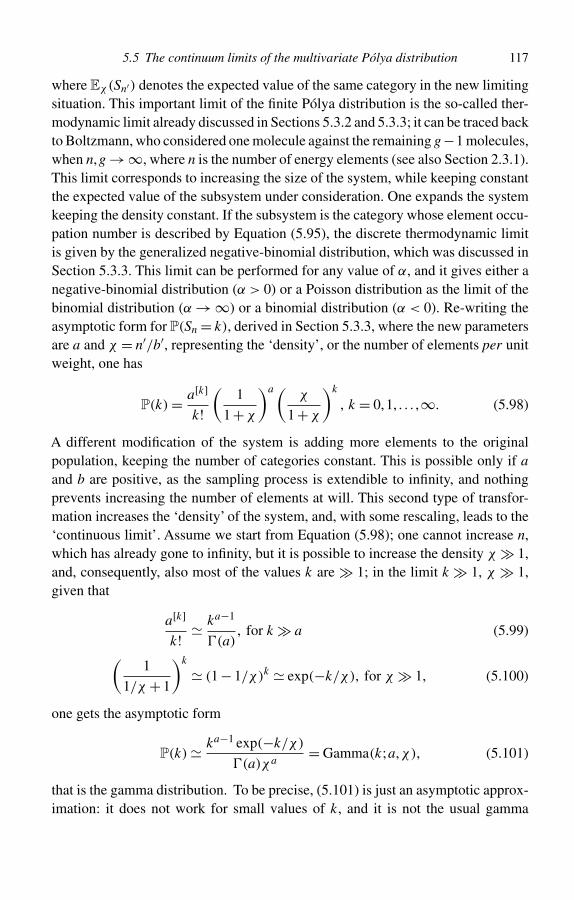
5.5 The continuum limits of the multivariate Pólya distribution 117
where Eχ(Sn′) denotes the expected value of the same category in the new limitingsituation. This important limit of the finite Pólya distribution is the so-called ther-modynamic limit already discussed in Sections 5.3.2 and 5.3.3; it can be traced backto Boltzmann, who considered one molecule against the remaining g −1 molecules,when n,g → ∞, where n is the number of energy elements (see also Section 2.3.1).This limit corresponds to increasing the size of the system, while keeping constantthe expected value of the subsystem under consideration. One expands the systemkeeping the density constant. If the subsystem is the category whose element occu-pation number is described by Equation (5.95), the discrete thermodynamic limitis given by the generalized negative-binomial distribution, which was discussed inSection 5.3.3. This limit can be performed for any value of α, and it gives either anegative-binomial distribution (α > 0) or a Poisson distribution as the limit of thebinomial distribution (α → ∞) or a binomial distribution (α < 0). Re-writing theasymptotic form for P(Sn = k), derived in Section 5.3.3, where the new parametersare a and χ = n′/b′, representing the ‘density’, or the number of elements per unitweight, one has
P(k) = a[k]
k!(
1
1 +χ
)a(χ
1 +χ
)k
, k = 0,1, . . . ,∞. (5.98)
A different modification of the system is adding more elements to the originalpopulation, keeping the number of categories constant. This is possible only if aand b are positive, as the sampling process is extendible to infinity, and nothingprevents increasing the number of elements at will. This second type of transfor-mation increases the ‘density’ of the system, and, with some rescaling, leads to the‘continuous limit’. Assume we start from Equation (5.98); one cannot increase n,which has already gone to infinity, but it is possible to increase the density χ � 1,and, consequently, also most of the values k are � 1; in the limit k � 1, χ � 1,given that
a[k]
k! ka−1
�(a), for k � a (5.99)(
1
1/χ + 1
)k
(1 − 1/χ)k exp(−k/χ), for χ � 1, (5.100)
one gets the asymptotic form
P(k) ka−1 exp(−k/χ)
�(a)χa= Gamma(k;a,χ), (5.101)
that is the gamma distribution. To be precise, (5.101) is just an asymptotic approx-imation: it does not work for small values of k, and it is not the usual gamma
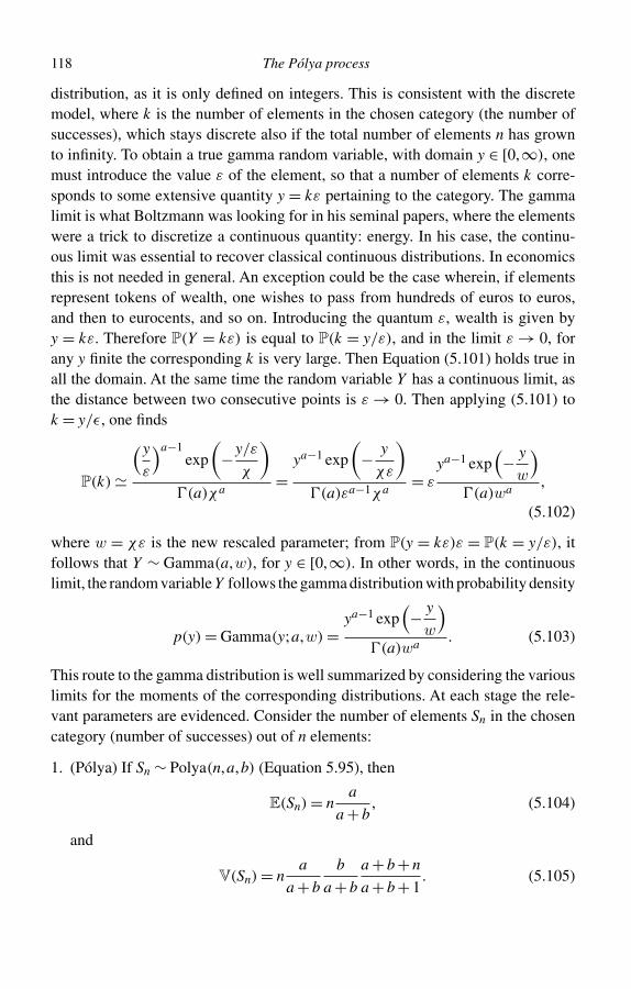
118 The Pólya process
distribution, as it is only defined on integers. This is consistent with the discretemodel, where k is the number of elements in the chosen category (the number ofsuccesses), which stays discrete also if the total number of elements n has grownto infinity. To obtain a true gamma random variable, with domain y ∈ [0,∞), onemust introduce the value ε of the element, so that a number of elements k corre-sponds to some extensive quantity y = kε pertaining to the category. The gammalimit is what Boltzmann was looking for in his seminal papers, where the elementswere a trick to discretize a continuous quantity: energy. In his case, the continu-ous limit was essential to recover classical continuous distributions. In economicsthis is not needed in general. An exception could be the case wherein, if elementsrepresent tokens of wealth, one wishes to pass from hundreds of euros to euros,and then to eurocents, and so on. Introducing the quantum ε, wealth is given byy = kε. Therefore P(Y = kε) is equal to P(k = y/ε), and in the limit ε → 0, forany y finite the corresponding k is very large. Then Equation (5.101) holds true inall the domain. At the same time the random variable Y has a continuous limit, asthe distance between two consecutive points is ε → 0. Then applying (5.101) tok = y/ε, one finds
P(k)
(y
ε
)a−1exp
(−y/ε
χ
)�(a)χa
=ya−1 exp
(− y
χε
)�(a)εa−1χa
= ε
ya−1 exp(− y
w
)�(a)wa
,
(5.102)
where w = χε is the new rescaled parameter; from P(y = kε)ε = P(k = y/ε), itfollows that Y ∼ Gamma(a,w), for y ∈ [0,∞). In other words, in the continuouslimit, the random variable Y follows the gamma distribution with probability density
p(y) = Gamma(y;a,w) =ya−1 exp
(− y
w
)�(a)wa
. (5.103)
This route to the gamma distribution is well summarized by considering the variouslimits for the moments of the corresponding distributions. At each stage the rele-vant parameters are evidenced. Consider the number of elements Sn in the chosencategory (number of successes) out of n elements:
1. (Pólya) If Sn ∼ Polya(n,a,b) (Equation 5.95), then
E(Sn) = na
a + b, (5.104)
and
V(Sn) = na
a + b
b
a + b
a + b + n
a + b + 1. (5.105)
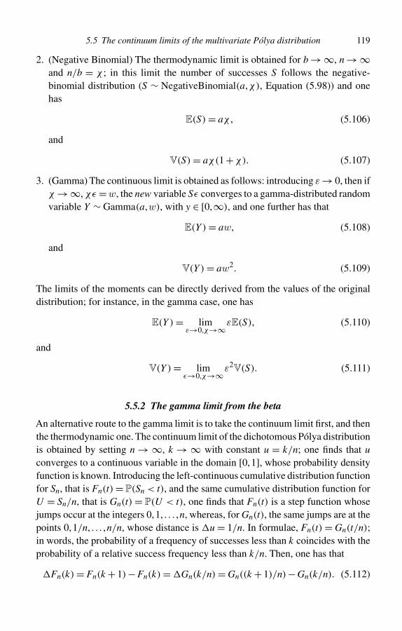
5.5 The continuum limits of the multivariate Pólya distribution 119
2. (Negative Binomial) The thermodynamic limit is obtained for b → ∞, n → ∞and n/b = χ ; in this limit the number of successes S follows the negative-binomial distribution (S ∼ NegativeBinomial(a,χ), Equation (5.98)) and onehas
E(S) = aχ , (5.106)
and
V(S) = aχ(1 +χ). (5.107)
3. (Gamma) The continuous limit is obtained as follows: introducing ε → 0, then ifχ → ∞, χε = w, the new variable Sε converges to a gamma-distributed randomvariable Y ∼ Gamma(a,w), with y ∈ [0,∞), and one further has that
E(Y ) = aw, (5.108)
and
V(Y ) = aw2. (5.109)
The limits of the moments can be directly derived from the values of the originaldistribution; for instance, in the gamma case, one has
E(Y ) = limε→0,χ→∞εE(S), (5.110)
and
V(Y ) = limε→0,χ→∞ε2V(S). (5.111)
5.5.2 The gamma limit from the beta
An alternative route to the gamma limit is to take the continuum limit first, and thenthe thermodynamic one. The continuum limit of the dichotomous Pólya distributionis obtained by setting n → ∞, k → ∞ with constant u = k/n; one finds that uconverges to a continuous variable in the domain [0,1], whose probability densityfunction is known. Introducing the left-continuous cumulative distribution functionfor Sn, that is Fn(t) = P(Sn < t), and the same cumulative distribution function forU = Sn/n, that is Gn(t) = P(U < t), one finds that Fn(t) is a step function whosejumps occur at the integers 0,1, . . . ,n, whereas, for Gn(t), the same jumps are at thepoints 0,1/n, . . . ,n/n, whose distance is u = 1/n. In formulae, Fn(t) = Gn(t/n);in words, the probability of a frequency of successes less than k coincides with theprobability of a relative success frequency less than k/n. Then, one has that
Fn(k) = Fn(k + 1)− Fn(k) = Gn(k/n) = Gn((k + 1)/n)− Gn(k/n). (5.112)
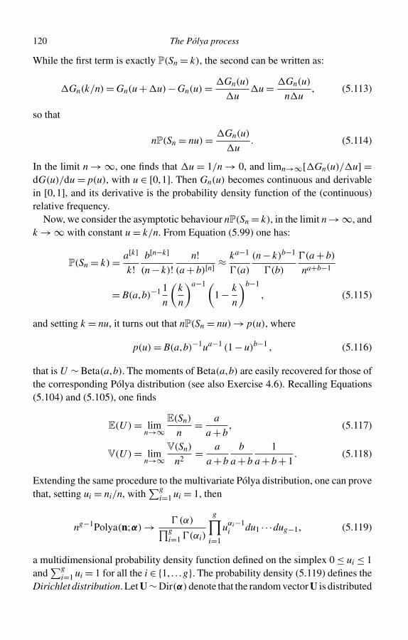
120 The Pólya process
While the first term is exactly P(Sn = k), the second can be written as:
Gn(k/n) = Gn(u + u)− Gn(u) = Gn(u)
u u = Gn(u)
n u, (5.113)
so that
nP(Sn = nu) = Gn(u)
u. (5.114)
In the limit n → ∞, one finds that u = 1/n → 0, and limn→∞[ Gn(u)/ u] =dG(u)/du = p(u), with u ∈ [0,1]. Then Gn(u) becomes continuous and derivablein [0,1], and its derivative is the probability density function of the (continuous)relative frequency.
Now, we consider the asymptotic behaviour nP(Sn = k), in the limit n → ∞, andk → ∞ with constant u = k/n. From Equation (5.99) one has:
P(Sn = k) = a[k]
k!b[n−k]
(n − k)!n!
(a + b)[n] ≈ ka−1
�(a)
(n − k)b−1
�(b)
�(a + b)
na+b−1
= B(a,b)−1 1
n
(k
n
)a−1(1 − k
n
)b−1
, (5.115)
and setting k = nu, it turns out that nP(Sn = nu) → p(u), where
p(u) = B(a,b)−1ua−1 (1 − u)b−1 , (5.116)
that is U ∼ Beta(a,b). The moments of Beta(a,b) are easily recovered for those ofthe corresponding Pólya distribution (see also Exercise 4.6). Recalling Equations(5.104) and (5.105), one finds
E(U ) = limn→∞
E(Sn)
n= a
a + b, (5.117)
V(U ) = limn→∞
V(Sn)
n2= a
a + b
b
a + b
1
a + b + 1. (5.118)
Extending the same procedure to the multivariate Pólya distribution, one can provethat, setting ui = ni/n, with
∑gi=1 ui = 1, then
ng−1Polya(n;α) → �(α)∏gi=1 �(αi)
g∏i=1
uαi−1i du1 · · ·dug−1, (5.119)
a multidimensional probability density function defined on the simplex 0 ≤ ui ≤ 1and
∑gi=1 ui = 1 for all the i ∈ {1, . . .g}. The probability density (5.119) defines the
Dirichlet distribution. Let U ∼ Dir(α) denote that the random vector U is distributed
5.5 The continuum limits of the multivariate Pólya distribution 121
according to the Dirichlet distribution of parameter vector α. As a consequenceof the Pólya label mixing property (Equation (5.36)), one immediately derivesthe aggregation property of the Dirichlet distribution. Note that U =U1, . . . ,Ug
is a sequence of random variables with values on the simplex∑g
i=1 ui with0 ≤ ui ≤ 1, ∀i ∈ {1, . . .g} whose joint distribution is Dir(α1, . . . ,αi, . . . ,αi+k , . . . ,αg).If one introduces UA =∑i+k
j=i Uj, then the new sequence (U1, . . . ,UA, . . . ,Ug) ∼Dir(α1, . . . ,αA, . . . ,αg), where αA = ∑i+k
j=i αj. The aggregation property imme-diately leads to the marginal distribution of the Dirichlet distribution, whoseprobability density function is nothing other than the beta distribution. If U ∼Dir(α1, . . . ,αg) then
Ui ∼ Beta(αi,α −αi). (5.120)
Here, a continuous variable was obtained introducing the relative frequency, whichis adimensional. Formally, the gamma limit of the beta distribution is straightfor-ward. If, in Equation (5.116), u is replaced by y/y0, and given that p(u) = g(y)y0,one gets:
g(y) = B(a,b)−1 1
y0
(y
y0
)a−1(1 − y
y0
)b−1
, (5.121)
for y ∈ [0,y0]; this is the probability density function of the so-called beta–Stacy dis-tribution Y ∼ betaStacy(a,b,y0). The beta–Stacy distribution, often used in modernBayesian statistics, is nothing other than the beta distribution rescaled on the intervaly ∈ [0,y0]. Now the gamma limit is obtained by letting y0 →∞, b →∞, and y0/b =χ remaining constant.Alittle thought is sufficient to see that, if no ‘quantum’is intro-duced, both y and y0 are integer numbers (they are nothing other than the old k andn), so that one ends with the same impasse as in Equation (5.101). In order to obtaina Gamma variable, with domain y ∈ [0,∞), one must restart from Equation (5.115)
P(Sn = k) �(a + b)
�(a)�(b)
1
n
(k
n
)a−1(1 − k
n
)b−1
, (5.122)
which works for k � 1 and n � 1. One introduces the value of the element again,so that total number of elements n corresponds to some extensive quantity nε = y0
and kε = y is the part pertaining to the category under scrutiny. Now if n → ∞,ε → 0, with nε = y0, then P(y = kε), with y ∈ [0,y0] converges to a continuousdistribution, and one finds the following probability density function:
g(y)ε B(a,b)−1 1
n
(k
n
)a−1(1 − k
n
)b−1
= B(a,b)−1 ε
y0
(y
y0
)a−1(1 − y
y0
)b−1
.
(5.123)
122 The Pólya process
Now, from Equations (5.99) and (5.100), and from the fact that for b � a one has
�(b + a)
�(b)ba= b[a]
ba→ 1, (5.124)
considering the limit y0 →∞, b →∞, with y0/b =w constant, one eventually finds
g(y) = Gamma(y;a,w) =ya−1 exp
(− y
w
)�(a)wa
, (5.125)
which coincides with p(y) in Equation (5.103).This alternative route to gamma is summarized by again considering the variouslimits and the moments of the corresponding distributions.At each stage the relevantparameters are indicated.
1. (Pólya) If Sn ∼ Polya(n,a,b) (Equation 5.95), then E(Sn) is given by Equation(5.104) and V(Sn) by Equation (5.105).
2. (Beta) The continuous limit is obtained as follows: if n → ∞, k → ∞ andk/n = u; then U ∼ beta(a,χ) and
E(U ) = a
a + b, (5.126)
V(U ) = a
a + b
b
a + b
1
a + b + 1. (5.127)
3. (Gamma) Finally, the thermodynamic limit is obtained as follows: introducingy = y0u, if b → ∞, y0 → ∞, with y0/b = w, the new variable y0U convergesto Y ∼ Gamma(a,w), with y ∈ [0,∞), and
E(Y ) = aw, (5.128)
V(Y ) = aw2. (5.129)
As before, the limits of the moments are directly derived by the previous values; inthe gamma case again, it is easy to check that
E(Y ) = limb→∞,y0→∞
y0E(U ), (5.130)
and
V(Y ) = limb→∞,y0→∞
y20V(U ). (5.131)
The scale factor of the gamma distribution is w, corresponding to the scale factor χ
of the negative-binomial distribution. Their intuitive meaning is that, if a categoryhas initial weight a, and the expected value of marginal variable is µ, then χ = µ/a
5.6 The fundamental representation theorem for the Pólya process 123
if the variable is the occupation number, or w = µ/a if the variable is the continuousmagnitude. In the example of Section 5.3.4, one has a = 1, b = g −1 and n/g = 5,that is the scale parameter of the negative-binomial approximation is equal to theaverage number of coins. When coins represent euros, NegativeBinomial(1,5) isjust Geometric(5) in the domain {0,1, . . . ,∞}. If an authority retires euros, andreplaces them with eurocents, whose distribution follows the same predictive prob-ability, now there are n′ = 100n coins in circulation, but the expected wealth isthe same. The new variable is closer to the continuous limit, and the numericalvalue of w is always equal to 5 euros = 500 cents. For ε → 0, the wealth isExponential(5)-distributed in the domain [0,∞).
5.5.3 Further remarks on the limits
The most important limit of the finite Pólya distribution is the thermodynamic limit,which corresponds to increasing the size (the number of categories) of the system,keeping the density constant, which is the expected value of the subsystem underconsideration. If the subsystem is a category whose occupation number is describedby Equation (5.95), the discrete thermodynamic limit is given by the generalizednegative-binomial distribution, which has been discussed in Section 5.3.3. Thislimit can be performed for any value of α, and it gives a usual negative-binomialdistribution (α > 0), a Poisson distribution (α →∞), or a binomial distribution (α <
0). If correlations are non-negative (α > 0), a continuous limit can be performed,whose meaning is increasing the density of elements. The continuum limit is auseful simplification of the high density case (large numbers of elements in fewcategories), or can be used to refine the degree of precision of finite magnitudes,reducing at will the ‘quanta’ assumed at the very beginning. This focus on theintroduction of continuous variables in an essentially discrete landscape can betraced back to Boltzmann’s deep conviction that the continuum is nothing other thana (sometimes) useful device to describe a world which is always finite and discrete.Among contemporary probability scholars, a similar deep conviction was sharedby E.T. Jaynes, who always underlined the importance of the limiting procedureleading to continuous quantities. His opinion can be summarized as follows: if onewishes to use continuous quantities, one must show the exact limiting procedurefrom the finite assumptions which are the necessary starting point.
5.6 The fundamental representation theorem for the Pólya process
The predictive form
P(Xm+1 = j|X(m)) = αj + mj
α + m, (5.132)
124 The Pólya process
whose historical root is in Laplace, has been justified from many points of viewin the past, without any appeal to urns and manipulation of balls. Given that, ina celebrated paper, Karl Pearson himself claimed that the fundamental problemin practical statistics is assigning probability to an event based on the empiricalevidence and the previous information, one can see that Equation (5.132) is apossible answer to the fundamental problem. It is usually justified (see Zabell,Further reading) following Johnson, a logician from Cambridge who was Keynes’teacher, under the postulate of sufficientness, which imposes that the predictiveform must depend only on the number of successes and the size of the sample, andnot on what happens in a failure. Johnson’s proof does not say anything in the caseof two categories, where the assumptions are trivial, and so it adds nothing to thebasic probability axioms. Followers of this approach are then always obliged tostate that the number of categories must be greater than two. Rudolph Carnap wentaround the obstacle, introducing an additional ‘linearity principle’ for the case ofonly two categories. A more satisfactory derivation, which works in any case, is dueto Costantini, later improved to encompass negative correlations. In the followingproof of the fundamental representation theorem in Costantini’s version (see Furtherreading, Chapter 4, Costantini (1979)), the symbol λ will be used instead of α,following Costantini, who used it just in memory of Carnap’s ‘λ-principle’. Theproof is based on the notion of relevance quotient, similar to the ‘coefficient ofinfluence’ introduced by Keynes. Here the proof is given in order to show also howit is possible to axiomatize a predictive probability, without introducing urn modelswhich can be used later just to interpret the probabilistic conditions.
Definition (Heterorelevance coefficient) The coefficient of heterorelevance ofcategory j with respect to i is
Qji(X
(m)) = P(Xm+2 = i|X(m),Xm+1 = j)
P(Xm+1 = i|X(m)), (5.133)
where P(Xm+1 = i|X(m)) gives the probability of observing category i at step m+1based on the observed evidence X(m). Note that Qj
i(X(m)) represent how a failure
j �= i at the (m + 1)th step influences the probability of observing the ith categoryat the (m + 2)th step. It is a measure for re-assessing the predictive probability fora category after a failure. Note that independence would imply Qj
i(X(m)) =1. In
terms of Qji(X
(m)), we can introduce the following conditions:
C1. Exchangeability (or symmetry) of Qji(X
(m)) with respect to the exchange of iand j, that is
Qji(X
(m)) = Qij(X
(m)). (5.134)
5.6 The fundamental representation theorem for the Pólya process 125
Indeed, C1 and (5.133) imply
P(Xm+1 = i,Xm+2 = j|X(m)) = P(Xm+1 = j,Xm+2 = i|X(m)), (5.135)
that is the recursive definition of exchangeability.
C2. Invariance of Qji(X
(m)), that is
Qji(X
(m)) =Qm. (5.136)
This means that, provided that i �= j, Qji(X
(m)) does not depend on either i and j,or on the evidence X(m); it is a function of m alone. If C2 holds true, then one canwrite
P(Xm+1 = i|X(m)) = p(i|mi,m), (5.137)
which represents Johnson’s sufficientness principle.
Theorem (Fundamental representation theorem for the Pólya process) If C2 holdstrue, that is Qj
i(X(m)) = Qm, then one has
P(Xm+1 = j|X(m)) = p(j|mj,m) = λpj + mj
λ+ m, (5.138)
where
λ = Q0
1 − Q0, (5.139)
and
pj = P(X1 = j). (5.140)
Proof Whatever the number g of categories, denote with a a given category,and with b its complement. Let p(a|m,s) represent the predictive probability thatthe (m + 1)th observation is in a after m successes and s trials. Equation (5.133)simplifies to
p(a|m,s + 1) = Qsp(a|m,s). (5.141)
For any evidence, denote with p(a|·) the predictive probability of the category, andwith p(b|·) = 1 − p(a|·) its complement. Note that predictive probabilities startingfrom ‘pure’ evidences such as (0,s) (all failures), or (s,s) (all successes), are easilywritten in terms of the initial probability pa = p(a|0,0) and of Q0, . . . ,Qs−1. Let usdenote by Q(r,t) the following product
Q(r,t) = QrQr+1 · . . . · Qt =t∏
i=r
Qi. (5.142)
126 The Pólya process
If the evidence is a sequence of only failures for the category under scrutiny, thenone has
p(a|0,s) = Q0Q1 · . . . · Qs−1p(a|0,0) = Q(0,s−1)pa; (5.143)
if the evidence is a sequence of all successes, then for the complementary categoryb they have been all failures, and one can write
p(b|0,s) = Q(0,s−1)pb. (5.144)
But, due to the fact that p(b|·) = 1 − p(a|·), one is led to
p(a|s,s) = 1 − p(b|0,s) = 1 − Q(0,s−1)(1 − pa) = 1 − Q(0,s−1) + Q(0,s−1)pa,(5.145)
where pa = 1 − pb has been used. Summarizing, one has
p(a|0,s) = Q(0,s−1)pa, (5.146)
p(a|s,s) = 1 − Q(0,s−1) + Q(0,s−1)pa. (5.147)
As for the generic predictive probability p(a|m,s), one is able to transport theinitial probability (pa,pb) along the borders of the allowed region of individualdescriptions, considering first the sequence
S1 = (a1, . . . ,am,bm+1, . . . ,bs), (5.148)
joining (0,0) to (m,s) through (m,m), and then the reversed sequence
S2 = (b1, . . . ,bs−m,as−m+1, . . . ,as), (5.149)
connecting (0,0) to (m,s) through (0,s − m).As for S1, the initial m successes give
p(a|m,m) = 1 − Q(0,m−1) + Q(0,m−1)pa. (5.150)
The next n − m failures give
p(a|m,s) = Q(m,s−1)p(a|m,m), (5.151)
leading to
p(a|m,s) = Q(m,s−1)(1 − Q(0,m−1) + Q(0,m−1)pa), (5.152)
and from
Q(0,m−1)Q(m,s−1) = Q(0,s−1), (5.153)
5.6 The fundamental representation theorem for the Pólya process 127
one can finally write
p(a|m,s) = Q(m,s−1) − Q(0,s−1) + Q(0,s−1)pa. (5.154)
By the same reasoning, for S2, one gets
p(b|s − m,s) = Q(s−m,s−1) − Q(0,s−1) + Q(0,s−1)pb. (5.155)
Considering the predictive distribution at (m,s), we have
p(a|m,s)+ p(b|s − m,s) = 1, (5.156)
so that the sum of Equations (5.154) and (5.155) leads to a recurrence relation onQ(m,s−1):
Q(m,s−1) − Q(0,s−1) + Q(0,s−1)pa + Q(s−m,s−1) − Q(0,s−1) + Q(0,s−1)pb = 1,(5.157)
from which, one finds
Q(m,s−1) + Q(s−m,s−1) − Q(0,s−1) = 1. (5.158)
The general solution of Equation (5.158) is
Q(m,s) = λ+ m
λ+ s + 1, (5.159)
and, eventually, one finds that
Qs = λ+ s
λ+ s + 1. (5.160)
Replacing (5.159) in (5.154), we get the thesis
p(a|m,s) = λ+ m
λ+ s− λ
λ+ s+ λpa
λ+ s= λpa + m
λ+ s, (5.161)
for m = 1, . . . ,s − 1. �
5.6.1 Remark on the recurrence formula
Considering that
Q(a,b) = QaQa+1 . . .Qb = Q(0,b)
Q(0,a−1)
, (5.162)
128 The Pólya process
the bidimensional equation (5.158) can be transformed into the unidimensionalrelation
Q(0,s−1)
Q(0,m−1)
+ Q(0,s−1)
Q(0,s−m−1)
− Q(0,s−1) = 1, (5.163)
and setting Q−1(0,a) = R(a), one gets
R(m − 1)+ R(s − m − 1) = 1 + R(s − 1). (5.164)
For instance, take the symmetric case m = s−m, that is s = 2m. Then R(2m−1) =2R(m − 1) − 1, which is satisfied only if R(x) is a linear function of x. PosingR(x) = a + bx, where
a = Q−10 = λ+ 1
λ, (5.165)
one gets a + b(2m − 1) = 2a + 2b(m − 1)− 1, and
b = a − 1 = 1
λ. (5.166)
Therefore, one has
R(s) = λ+ 1
λ+ s
λ= λ+ s + 1
λ, (5.167)
and
Q(0,s) = λ
λ+ s + 1. (5.168)
One finds that
R(s) = λ+ s + 1
λ, (5.169)
satisfies (5.164) for any 1 ≤ m ≤ s − 1, as is easily verified.
5.6.2 Remarks on the fundamental theorem
The main applications of Equation (5.1) were in the field of predictive inference.Therefore, the case α > 0 was mainly studied, which is the usual Pólya case. Ifα > 0, then, using αj = αpj, the ratio (αpj + mj)/(λ + m) is always positive, andthe n-step process can be extended to infinity; moreover, any frequency vector(mj,m) can be reached from (0,0) with positive probability (except in the trivialcase pj = 0, that is not considered here). Now one has that α = Q0/(1 − Q0), and
5.6 The fundamental representation theorem for the Pólya process 129
Q0 =α/(α+1), and Qs = (α+s)/(α+s+1); therefore a positive α implies Qs < 1.This is not surprising, because if the observations are positively correlated, after afailure the predictive probability decreases. If α → ∞, then one gets Q0 → 1, anda failure does not influence the predictive probability in the next trial. In the caseα → 0, it turns out that Q0 → 0; this means that if a category does not appear inthe first trial, in the second trial it becomes almost impossible to see it. Then, in thelimit α → 0, one expects to see ‘pure states’ almost exclusively. If α = 0 the firstcategory determines all the future process, which is no longer probabilistic afterthe first trial. Only occupation vectors of the form (0, . . . ,0,s,0, . . . ,0) are possible.For this reason, the value α = 0 was refused by Carnap. Remarkably, α = 0 leadsto the frequentist view of probability, where the predictive rule is
P(Xm+1 = j|X(m)) = mj
m. (5.170)
This difficulty is only overcome in the following limit m � α < ∞, when
λpj + mj
λ+ m mj
m. (5.171)
That the predictive form (αpj + mj)/(α + m) is richer of consequences than itsfrequentist counterpart is evident when writing
αpj + mj
α + m=
αpj + mmj
mα + m
, (5.172)
where α and m are understood as weights applied to pj (the prior probability) andmj/m (the empirical frequency distribution). Therefore, the predictive probabilityis a weighted average of the initial probability (with weight α) and of the frequencydistribution (with weight m). One can imagine that the predictive assignment resultsin two stages: the first step is choosing either the initial probability t with prob-ability α/(α + m) or the empirical distribution e with probability m/(α + m); thesecond step is selecting from the chosen distribution, with probability pj or mj/m,respectively. In formulae
P(Xm+1 = j|·) = P(Xm+1 = j|t, ·)P(t|·)+P(Xm+1 = j|e, ·)P(e|·), (5.173)
where
P(t|·) = α
α + m, P(e|·) = m
α + m, (5.174)
and
P(Xm+1 = j|t, ·) = pj, P(Xm+1 = j|e, ·) = mj
m. (5.175)
130 The Pólya process
Then a large value of α means a small influence of the empirical distribution,whereas a small value of α means a large influence of the already accommodatedunits on the choice of the new object leading to a sort of herding behaviour.
Some caution is needed in the case α < 0. The general form
|α|pj − mj
|α|− m, (5.176)
evidences that |α| is the maximum number of possible observations and that |α|pj
must be integer, in order to satisfy probability axioms. Equation (5.146) means thatthe prior probability pj multiplied by the coefficient Q(0,s−1) gives the probabilityof observing the jth category at the next step after having observed failures only.In the case under scrutiny, one has
Qs = |α|− s
|α|− s − 1> 1; (5.177)
therefore, as a consequence of Equation (5.146), one arrives at
Q(0,s) = |α||α|− s − 1
> 1. (5.178)
Thus p(j|0,s) = Q(0,s −1)pj increases with s. There must be an s∗ : p(j|0,s∗) = 1,and p(B|0,s∗) = 0, where B represents the set of all categories not coinciding withj. It is intuitive that s∗ = |α|pB = |α|(1 − pj), which must be integer. Now, if oneconsiders p(B|0,s) one reaches the same conclusion leading to the fact that |α|pj isinteger. The domain of definition of p(j|mj,s) is such that the possible frequencyvectors are those crossed by the sequences connecting (0,0) to (|α|pj, |α|(1−pj)).
5.7 Exercises
5.1 Prove that
E(X1 + X2) = E(X1)+E(X2). (5.179)
5.2 Prove that
V(X1 + X2) = V(X1)+V(X2)+ 2C(X1,X2). (5.180)
5.3 Prove that
E(I (k)i I (k)
j ) = P(Xi = k,Xj = k). (5.181)
5.4 Consider a dichotomous Pólya process with parameters α0 and α1 and definethe random variable Y (m) = +1 if X (m) = 1 and Y (m) = −1 if X (m) = 0. Inother words, one has
Y = 2X − 1. (5.182)
5.8 Summary 131
Then define the random variable S(m) (Pólya random walk) as
S(m) =m∑
i=1
Y (i). (5.183)
Write a program that simulates the Pólya random walk and discuss someinteresting cases.
5.5 In the previous exercise, a qualitative discussion was presented for the binomiallimit of the dichotomous Pólya distribution. But how close is the symmetricdichotomous Pólya to the binomial distribution when α0 = α1 = 100? Try toanswer this question by means of a Monte Carlo simulation.
5.6 A classical problem in probability theory is often stated as follows. Imaginethere are n persons in a room, with n < 365. What is the probability that atleast two of them have a common birthday? This problem and indeed manyother problems related to the birthday distribution can be solved by means ofthe method discussed in Section 5.3.8. How?
5.8 Summary
In this chapter, the Pólya process and the corresponding generalized multivariatePólya distribution were analyzed in detail. The Pólya process is an exchangeableprocess whose predictive probability is a mixture of a priori probability and of theobserved frequency for the category under scrutiny.
The generalized multivariate Pólya sampling distribution encompasses manywell-known distributions including the multinomial distribution and the multivari-ate hypergeometric distribution. In the thermodynamic limit, the generalized Pólyabecomes the generalized negative binomial, encompassing the Poisson distribution(α → ∞). For positive α, the continuous limit of the multivariate Pólya distribu-tion is the Dirichlet distribution and its marginal distribution is the beta distributionalready discussed in Section 4.4. The thermodynamic limit of the beta is the gammadistribution.
Due to exchangeability on the frequency vectors, from the multivariate gener-alized Pólya distribution one can derive the probability of partition vectors. Thisprobability can be marginalized and the mathematical expectation of any com-ponent of the partition vector can be obtained. Exemplified in Section 5.3.8, thisprocedure will often be used in the following chapters.
Based on Lagrange multipliers, an alternative method allows us to determine themost probable partition vector. Also this procedure will be used further in this book.
The invariance of the heterorelevance coefficient defined in Section 5.6 is asufficient condition for obtaining the predictive probability characterizing the Pólya
132 The Pólya process
process. This provides a complete characterization for this class of exchangeablestochastic processes.
Further reading
Pearson states the fundamental problem of practical statistics as follows:
An ‘event’has occurred p times out of p+q = n trials, where we have no a priori knowledgeof the frequency of the event in the total population of occurrences. What is the probabilityof its occurring r times in a further r + s = m trials?
The reader can consult the following paper:
K. Pearson, The Fundamental Problem of Practical Statistics, Biometrika, 13 (1), 1–16(1920).
Johnson’s original paper on the sufficientness postulate:
W.E. Johnson, Probability: the Deductive and Inductive Problem, Mind, 49, 409–423(1932).
is discussed in a paper by Zabell:
S.L. Zabell, W.E. Johnson’s “Sufficientness” Postulate, The Annals of Statistics, 10 (4),1090–1099 (1982).
Johnson’s paper was published posthumously. The term sufficientness postulatewas introduced by I.J. Good, who first used the expression sufficiency postulateand later used sufficientness to avoid confusion with the usual statistical meaningof sufficiency:
I.J. Good, The Estimation of Probabilities: An Essay on Modern Bayesian Methods, MITPress, Research Monograph No. 30 (1965).
Zabell completed the proof sketched in Johnson’s paper. Note that Johnson’ssufficientness postulate assumes that
P(Xm+1 = j|X1 = x1, . . . ,Xm = xm) = fj(mj); (5.184)
therefore, originally, it was not a condition on the heterorelevance coefficient. Notethat the postulate is vacuous for g = 2 and a further assumption of linearity isnecessary in the dichotomous case in order to derive the fundamental theorem.Costantini’s paper on the heterorelevance coefficient is listed in further reading inChapter 4.
According to Zabell, Carnap and his collaborators independently rediscoveredvarious results due to Johnson. The dichotomous case and the linearity assumptionare discussed in a book by Carnap and Stegmüller:
5.8 Summary 133
R. Carnap and W. Stegmüller, Induktive Logik und Wahrscheinlichkeit, Springer, Vienna(1959).
W. Brian Arthur used the Pólya distribution in economics. This application isdiscussed in the following book:
W. Brian Arthur, Increasing Returns and Path Dependence in the Economy, The Universityof Michigan Press, Ann Arbor MI (1994).
A website is available with applets and exercises on the Pólya urn scheme
http://www.math.uah.edu/stat.
6
Time evolution and finite Markov chains
Up to now, index set I for a stochastic process can indifferently denote eithersuccessive draws from an urn or a time step in a time evolution. In this chapter,a probabilistic dynamics for n objects divided into g categories will be defined.The simplest case is Markovian dynamics in discrete time, and so this chapter isdevoted to the theory of finite Markov chains.
After studying this chapter you should be able to:
• define Markov chains;• discuss some properties of Markov chains such as irreducibility, periodicity,
stationarity and reversibility;• determine the invariant distribution for Markov chains either by means of the
Markov equation or by using Monte Carlo simulations;• understand the meaning of statistical equilibrium for aperiodic irreducible
Markov chains;• use the detailed balance principle to compute the invariant distribution, if
possible;• exemplify the above properties using the Ehrenfest urn as a prototypical Markov
chain.
6.1 From kinematics to Markovian probabilistic dynamics
6.1.1 Kinematics
Consider a population composed of n elements and g categories which partitionthe variate under study. In economics, the n elements may represent economicagents and the g categories can be seen as strategies, but other interpretationsare possible. For instance, one can speak of n individuals working in g factoriesor n firms active in g economic sectors, and so on. In physics, the n elementsmay be particles and the g categories energy levels or, following Boltzmann, onecan consider n energy elements to be divided into g particles, etc. In any case,
134
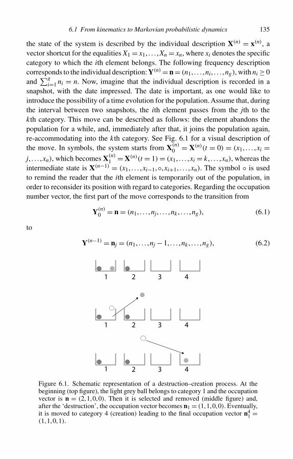
6.1 From kinematics to Markovian probabilistic dynamics 135
the state of the system is described by the individual description X(n) = x(n), avector shortcut for the equalities X1 = x1, . . . ,Xn = xn, where xi denotes the specificcategory to which the ith element belongs. The following frequency descriptioncorresponds to the individual description: Y(n) = n = (n1, . . . ,ni, . . . ,ng), with ni ≥ 0and
∑gi=1 ni = n. Now, imagine that the individual description is recorded in a
snapshot, with the date impressed. The date is important, as one would like tointroduce the possibility of a time evolution for the population. Assume that, duringthe interval between two snapshots, the ith element passes from the jth to thekth category. This move can be described as follows: the element abandons thepopulation for a while, and, immediately after that, it joins the population again,re-accommodating into the kth category. See Fig. 6.1 for a visual description ofthe move. In symbols, the system starts from X(n)
0 = X(n)(t = 0) = (x1, . . . ,xi =j, . . . ,xn), which becomes X(n)
1 = X(n)(t = 1) = (x1, . . . ,xi = k, . . . ,xn), whereas theintermediate state is X(n−1) = (x1, . . . ,xi−1,◦,xi+1, . . . ,xn). The symbol ◦ is usedto remind the reader that the ith element is temporarily out of the population, inorder to reconsider its position with regard to categories. Regarding the occupationnumber vector, the first part of the move corresponds to the transition from
Y(n)0 = n = (n1, . . . ,nj, . . . ,nk , . . . ,ng), (6.1)
to
Y(n−1) = nj = (n1, . . . ,nj − 1, . . . ,nk , . . . ,ng), (6.2)
1 2 3 4
1 2 3 4
1 2 3 4
Figure 6.1. Schematic representation of a destruction–creation process. At thebeginning (top figure), the light grey ball belongs to category 1 and the occupationvector is n = (2,1,0,0). Then it is selected and removed (middle figure) and,after the ‘destruction’, the occupation vector becomes n1 = (1,1,0,0). Eventually,it is moved to category 4 (creation) leading to the final occupation vector n4
1 =(1,1,0,1).
136 Time evolution and finite Markov chains
that is the destruction of an element in the jth category. The second part is thetransition from nj = (n1, . . . ,nj − 1, . . . ,nk , . . . ,ng) to
Y(n)1 = nk
j = (n1, . . . ,nj − 1, . . . ,nk + 1, . . . ,ng), (6.3)
that is a creation of an element in the kth category. The kinematics is modelledto describe the category changes of the n elements. At each time step, one canimagine that an element is selected, and temporarily abandons the system; after this‘destruction’, the same agent re-accommodates into the site system (‘creation’). Ifthe final category is different from the initial one a category change takes place. Sucha move can be straightforwardly generalized assuming that m agents are selected ina sequence, and then they re-accommodate in a sequence within the time intervalfrom t to t + 1. Then the size of the population shrinks as long as the selectionoccurs, and it gradually returns to the original size after all the accommodations.Due to this shrinking–enlarging of the population it is useful to define more preciselythe random variable called occupation number vector as Y(n) = (y(n)
1 , . . . ,y(n)g ) =
(N1,n, . . . ,Ng,n), with∑g
i=1 y(n)i = n.
6.1.2 Example: seven dice on a table
Consider seven different dice showing their upper face in the following sequence:X(7)
0 = (2,6,2,1,1,5,4). Then Y(7)0 = (2,2,0,1,1,1), because 1 and 2 appear twice,
4, 5, and 6 appear once, whereas 3 is not present. Now, the third die is removed,before being re-cast, the individual description becomes X(6) = (2,6,◦,1,1,5,4),and the frequency description is Y(6) = (2,1,0,1,1,1). After the third die has beencast, imagine it displays a 1; therefore, one has that X(7)
1 = (2,6,1,1,1,5,4), and
Y(7)1 = (3,1,0,1,1,1). In summary, one has:
X(7)0 = (2,6,2,1,1,5,4); Y(7)
0 = (2,2,0,1,1,1);6∑
i=1
y(7)i = 7
X(6) = (2,6,◦,1,1,5,4); Y(6) = (2,1,0,1,1,1);6∑
i=1
y(6)i = 6
X(7)1 = (2,6,1,1,1,5,4); Y(7)
1 = (3,1,0,1,1,1).6∑
i=1
y(7)i = 7. (6.4)
Note that X(7)1 differs from X(7)
0 in that the third element has changed from category 2to category 1. As far as the occupation number description is concerned: an elementwas removed (destroyed) from the second category and an element was added
6.1 From kinematics to Markovian probabilistic dynamics 137
(created) to the first category. If the same operation is repeated, that is a die is picked,and then it is re-cast, and the new situation is recorded (by means of an individualor a statistical vector), after at most 7 trials all possible situations can be reached.Of these situations the most extreme case is X(7) = (3,3,3,3,3,3,3), correspondingto Y(7) = (0,0,7,0,0,0). In fact starting from X(7)
0 = (2,6,2,1,1,5,4), Y(7)(0) =(2,2,0,1,1,1) one has to pick all 7 dice in a row, and always get the result 3.(Note that a possibility is considered, even if this possibility would appear veryimprobable.)
6.1.3 Individual and/or statistical descriptions
The individual description is a sequence as long as the size of the population n,whereas the statistical description is usually much shorter; in other words, one oftenhas g � n. For instance, if the number of dice in the previous example were 1010 (anorder of magnitude typical of economic populations), their statistical descriptionwould continue to be a 6-dimensional vector. Even if, in principle, nothing pre-vents following the time evolution of the individual description (see the exampleof the Ehrenfest urn model below), focusing on a statistical description is not onlypractical, but is also a consequence of the probabilistic dynamics. Indeed, if theprobabilistic time evolution is not distinguishing the individual names, a statisticaldescription is enough to study all the relevant properties of the evolving population.Further, consider that economic concepts such as the income distribution, the GDP,and so on are statistical in character. Hence, it is natural to define as the state of thesystem at time step t, its statistical distribution Y(n)
t . The superscript can be omitted,simply writing Yt when no confusion is possible. The state space is then the set ofg-ples summing up to n, denoted by Sn
g = Y U = {(n1, . . . ,ng), ni ≥ 0,∑
ni = n}. Thediscrete-time evolution is represented by the sequence Y0,Y1, . . . ,Ys, . . ., where Ys
is an element of Sng = Y U . A sequence is a possible history of the population, and it
can be conceived as a realization of a stochastic process, if the dynamics is proba-bilistic. If each change from Ys to Ys+1 is probabilistic, and the transition probabilityonly depends on the state Ys and not on the full history Ys−1,Ys−2, . . . ,Y0, the prob-abilistic dynamics is said to be a Markov chain, whose transition probability is amatrix of elements P(Yt+1 = n′|Yt = n) = w
(n,n′) , n′,n ∈Sn
g . If these matrix ele-ments do not depend on time t, the Markov chain is called homogeneous. Thischapter is devoted to the theory of homogeneous Markov chains.
6.1.4 A Markov chain for the seven dice
Referring to the previous example of dice casting, assume that at each time step adie is chosen at random (all dice being on a par); then it is cast, and the probability
138 Time evolution and finite Markov chains
of each result is 1/6 for any die. Let Y(7)0 = (2,2,0,1,1,1) = n. The probability
that a die is selected belonging to the ith category is then ni/n. The probability ofgetting the intermediate state Y(6) = (2,1,0,1,1,1) = n2 = (n1,n2 − 1, . . . ,n6) is2/7. Casting this die (it was the third one), the probability of obtaining a 1 is 1/6.Then, one finds P(Y(7)
1 = (3,1,0,1,1,1)| Y(7)0 = (2,2,0,1,1,1)) = (2/7)(1/6) =
1/21. By means of the same procedure, one can determine the transition probabilityP(Yt+1 = n′|Yt = n), where n′ = nj
i = (n1, . . . ,ni − 1, . . . ,nj + 1, . . . ,n6); this isgiven by
P(Yt+1 = nji|Yt = n) = ni
n
1
6, j �= i. (6.5)
If j �= i, a true change takes place, and this can occur in only one way (selecting adie displaying an i which results in a die displaying a j after being cast). But thedie could end in the same category as it was before being selected, in this case,n′ = n, and this can occur in 6 alternative ways, each of them through a differentdestruction ni, i = 1, . . . ,6. More formally, it is useful to write the two parts ofEquation (6.5) separately. If j �= i, then P(Yt+1 = nj
i|Yt = n) = P(ni|n)P(nji|ni),
where P(ni|n) = ni/n is the destruction term, transforming a vector Y(n) of size ninto a vector Y(n−1), whereas the creation term P(nj
i|ni) transforms a vector Y(n−1)
of size n − 1 into a vector Y(n). Then the probability of no change can be writtenas follows:
P(Yt+1 = n|Yt = n) =6∑
i=1
P(ni|n)P(nii|ni) =
6∑i=1
ni
n
1
6= 1
6. (6.6)
Given the rules of the game, all possible sequences of states are those sequences ofconsecutive occupation numbers differing by no more than two components, that is
|n′ − n| =g∑
i=1
|n′i − ni| ∈ {0,2}, (6.7)
where 2 denotes a true change and 0 no change. Then, given the initial state anypossible sequence Y1, . . . ,Yt|Y0 has probability
P(Y1 = y1|Y0 = y0)P(Y2 = y2|Y1 = y1) · · ·P(Yt = yt|Yt−1 = yt−1), (6.8)
where each term comes from (6.5) if |yt −yt−1|= 2, and from (6.6) if |yt −yt−1|= 0.Therefore, in this game, the probability of every event can be determined.
Interesting quantities are objects such as P(Yt = n′|Y0 = n) when t is verylarge, whose meaning is the probability of the states that can be observed aftermany moves. Formally, one can calculate P(Yt = n′|Y0 = n) adding the probability
6.2 The Ehrenfest urn model 139
of all sequences Y1, . . . ,Yt−1 connecting Y0 = n to Yt = n′. But a little thoughtis enough to see that, after a number of trials large compared with the numberof dice, all dice will be selected at least once, so that their initial state will becancelled. As they have been recast once at least, an observer that has turned his/herhead and has missed all values of Y1, . . . ,Yt−1, when turning to the table again,is going to observe seven dice which were cast, the number of castings beingirrelevant. It is quite reasonable to expect that the probability of the states willbe governed by a P(Yt = n′|Y0 = n) which does not depend on Y0, and thatlimt→∞ P(Yt = n′|Y0 = n) = π(n′) is the usual multinomial distribution whichdescribes casting of seven fair dice. In the following, it will be shown that the chainindeed reaches its equilibrium distribution π(n′).
Another interesting statistical property is the fraction of time in which the systemvisits any given state as time goes by. For instance, considering the state y =(6,0,0,0,0,0) where all the dice display a 1, its visiting fraction is the randomvariable counting the number of times in which all the dice show 1 divided bythe total number of trials. It can be shown that the fraction of visits to any stateconverges (in probabilistic terms) for t → ∞, and the limiting value is just π(n),its probability of being observed at a large but fixed time. This property (also calledergodicity), appearing rather commonsensical for probabilistic systems such asthe one under scrutiny, is very important in the foundations of classical statisticalmechanics based on Newton’s deterministic dynamics.
6.2 The Ehrenfest urn model
In the words of Kac, the Ehrenfest urn model is ‘probably one of the most instructivemodels in the whole of Physics’ (see Further reading at the end of the chapter). Itwas designed to support a probabilistic vindication of Boltzmann’s H -theorem, andto give a qualitative account of notions like reversibility, periodicity and tendencyto equilibrium (concepts that will be further explained below). The model, oftenreferred to as the ‘Ehrenfest dog-flea model’, is mentioned in many textbooks onprobability, stochastic processes and statistical physics. It is probably the simplestrandom walk with reflecting barriers where increments are dependent on the stateof the system and it is an example of a birth–death process which is a homoge-neous Markov chain. For a birth–death Markov chain only the following transitionprobabilities are non-vanishing: w(i, i + 1) (birth), w(i, i − 1) (death) and w(i, i).Considering fleas and dogs, in an informal way, one has g = 2 dogs and n fleas, ofwhich i are on the first dog and (n − i) on the second. At each discrete time step aninteger number between 1 and n is chosen at random, and the corresponding flea isforced to hop towards the other dog. This mechanism can be formalized as follows.A discrete stochastic process {Yt}t≥0 = Y0,Y1, . . . ,Yt , . . . is introduced whose values
140 Time evolution and finite Markov chains
are in Y U = (0, . . . , i, . . . ,n), representing the occupation number of, or the numberof balls in, the first urn (or the number of fleas on the first dog) at time t. The state ofthe system is thus represented by the ordered pair (i,n− i). From the rule describedin words, the transition probability is modified as follows
w(i, i + 1) = P(Yt+1 = i + 1|Yt = i) = n − i
n, i = 0, . . . ,n − 1
w(i, i − 1) = P(Yt+1 = i − 1|Yt = i) = i
n. i = 1, . . . ,n. (6.9)
Note that in all the other cases w(i, j) = P(Yt+1 = j|Yt = i) = 0 and that one has∑j w (i, j) = 1. Most of the mathematical complications of the model are a con-
sequence of the fact that the randomly chosen flea is forced to change dog. Thisimplies that, at each transition, if i was even it must change into an odd number, andvice versa. Thus, the parity is conserved after two transitions, and this constraint isnot cancelled by the time evolution. Therefore, the probability of finding an evennumber oscillates from a positive number (for even steps) to zero (for odd steps),and this holds forever. By means of a slight modification of the model, this peri-odicity can be avoided. It is enough to let the selected flea return to the dog fromwhich it came. Assume that a flea on the first dog is selected and then hops on to thesecond dog. The dog occupation vector passes from the initial state (i,n− i), to theintermediate state (i −1,n− i); eventually, there is the transition from (i −1,n− i)to (i − 1,n − i + 1), the final state. Using the physical jargon introduced above,this transition is equivalent to the destruction of a flea on the first dog, followedby the creation of a flea on the second. In statistical jargon this may describe thefact that an element changes category. Now, if the flea can also come back to theoriginal dog, instead, one has the transition (i,n − i) → (i − 1,n − i) → (i,n − i),that is the final state does coincide with the initial one. If the creation probabilityis symmetric, Equation (6.9) becomes
w(i, i + 1) = P(Yt+1 = i + 1|Yt = i) = n − i
n
1
2, i = 0, . . . ,n − 1
w(i, i) = P(Yt+1 = i|Yt = i) = 1
2, i = 0, . . . ,n
w(i, i − 1) = P(Yt+1 = i − 1|Yt = i) = i
n
1
2, i = 1, . . . ,n. (6.10)
Again, all the other cases are forbidden transitions and their probability is 0. Thisprocess is a simplification of the previous dice process. Equation (6.10) describes ncoins on the table, a coin is picked at random and then tossed, so that Yt = i denotesthat, after t moves, there are i coins displaying heads and n − i coins displayingtails. Repeating the previous considerations, one can show that the equilibrium
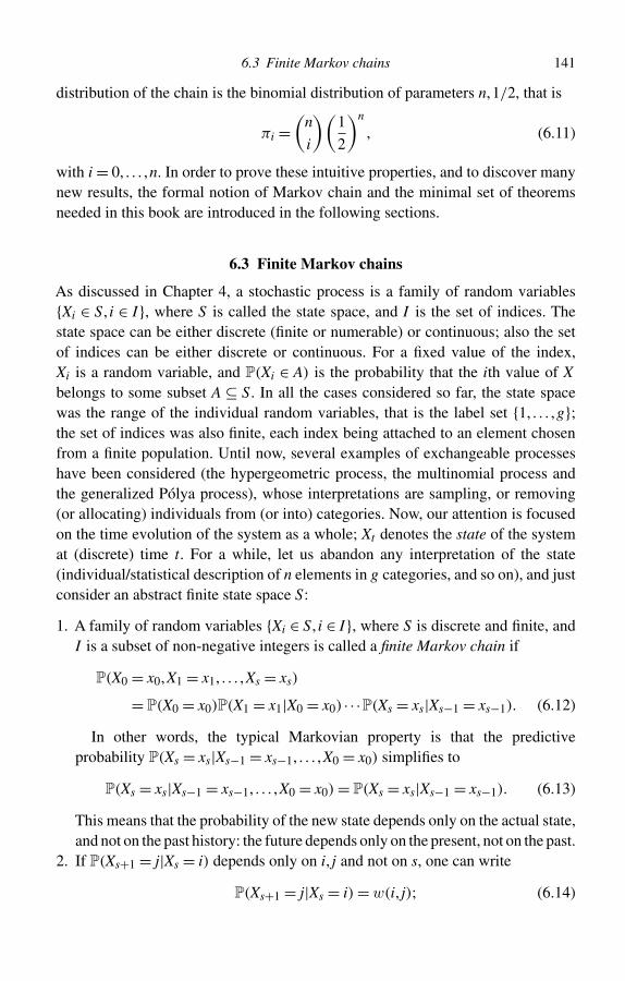
6.3 Finite Markov chains 141
distribution of the chain is the binomial distribution of parameters n,1/2, that is
πi =(
n
i
)(1
2
)n
, (6.11)
with i = 0, . . . ,n. In order to prove these intuitive properties, and to discover manynew results, the formal notion of Markov chain and the minimal set of theoremsneeded in this book are introduced in the following sections.
6.3 Finite Markov chains
As discussed in Chapter 4, a stochastic process is a family of random variables{Xi ∈ S, i ∈ I}, where S is called the state space, and I is the set of indices. Thestate space can be either discrete (finite or numerable) or continuous; also the setof indices can be either discrete or continuous. For a fixed value of the index,Xi is a random variable, and P(Xi ∈ A) is the probability that the ith value of Xbelongs to some subset A ⊆ S. In all the cases considered so far, the state spacewas the range of the individual random variables, that is the label set {1, . . . ,g};the set of indices was also finite, each index being attached to an element chosenfrom a finite population. Until now, several examples of exchangeable processeshave been considered (the hypergeometric process, the multinomial process andthe generalized Pólya process), whose interpretations are sampling, or removing(or allocating) individuals from (or into) categories. Now, our attention is focusedon the time evolution of the system as a whole; Xt denotes the state of the systemat (discrete) time t. For a while, let us abandon any interpretation of the state(individual/statistical description of n elements in g categories, and so on), and justconsider an abstract finite state space S:
1. A family of random variables {Xi ∈ S, i ∈ I}, where S is discrete and finite, andI is a subset of non-negative integers is called a finite Markov chain if
P(X0 = x0,X1 = x1, . . . ,Xs = xs)
= P(X0 = x0)P(X1 = x1|X0 = x0) · · ·P(Xs = xs|Xs−1 = xs−1). (6.12)
In other words, the typical Markovian property is that the predictiveprobability P(Xs = xs|Xs−1 = xs−1, . . . ,X0 = x0) simplifies to
P(Xs = xs|Xs−1 = xs−1, . . . ,X0 = x0) = P(Xs = xs|Xs−1 = xs−1). (6.13)
This means that the probability of the new state depends only on the actual state,and not on the past history: the future depends only on the present, not on the past.
2. If P(Xs+1 = j|Xs = i) depends only on i, j and not on s, one can write
P(Xs+1 = j|Xs = i) = w(i, j); (6.14)
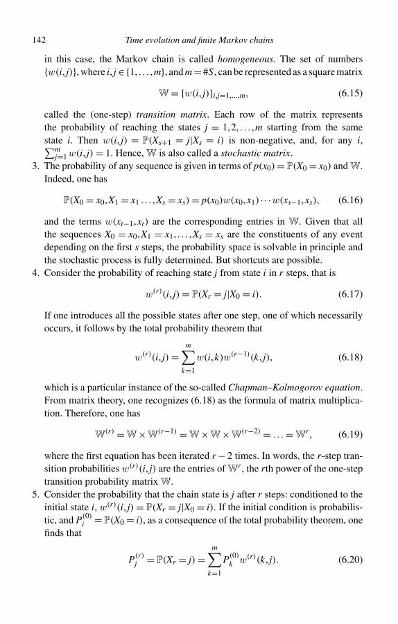
142 Time evolution and finite Markov chains
in this case, the Markov chain is called homogeneous. The set of numbers{w(i, j)}, where i, j ∈ {1, . . . ,m}, and m = #S, can be represented as a square matrix
W = {w(i, j)}i,j=1,...,m, (6.15)
called the (one-step) transition matrix. Each row of the matrix representsthe probability of reaching the states j = 1,2, . . . ,m starting from the samestate i. Then w(i, j) = P(Xs+1 = j|Xs = i) is non-negative, and, for any i,∑m
j=1 w(i, j) = 1. Hence, W is also called a stochastic matrix.3. The probability of any sequence is given in terms of p(x0) = P(X0 = x0) and W.
Indeed, one has
P(X0 = x0,X1 = x1 . . . ,Xs = xs) = p(x0)w(x0,x1) · · ·w(xs−1,xs), (6.16)
and the terms w(xt−1,xt) are the corresponding entries in W. Given that allthe sequences X0 = x0,X1 = x1, . . . ,Xs = xs are the constituents of any eventdepending on the first s steps, the probability space is solvable in principle andthe stochastic process is fully determined. But shortcuts are possible.
4. Consider the probability of reaching state j from state i in r steps, that is
w(r)(i, j) = P(Xr = j|X0 = i). (6.17)
If one introduces all the possible states after one step, one of which necessarilyoccurs, it follows by the total probability theorem that
w(r)(i, j) =m∑
k=1
w(i,k)w(r−1)(k, j), (6.18)
which is a particular instance of the so-called Chapman–Kolmogorov equation.From matrix theory, one recognizes (6.18) as the formula of matrix multiplica-tion. Therefore, one has
W(r) = W×W(r−1) = W×W×W(r−2) = . . . = Wr , (6.19)
where the first equation has been iterated r − 2 times. In words, the r-step tran-sition probabilities w(r)(i, j) are the entries of Wr , the rth power of the one-steptransition probability matrix W.
5. Consider the probability that the chain state is j after r steps: conditioned to theinitial state i, w(r)(i, j) = P(Xr = j|X0 = i). If the initial condition is probabilis-tic, and P(0)
i = P(X0 = i), as a consequence of the total probability theorem, onefinds that
P(r)j = P(Xr = j) =
m∑k=1
P(0)k w(r)(k, j). (6.20)
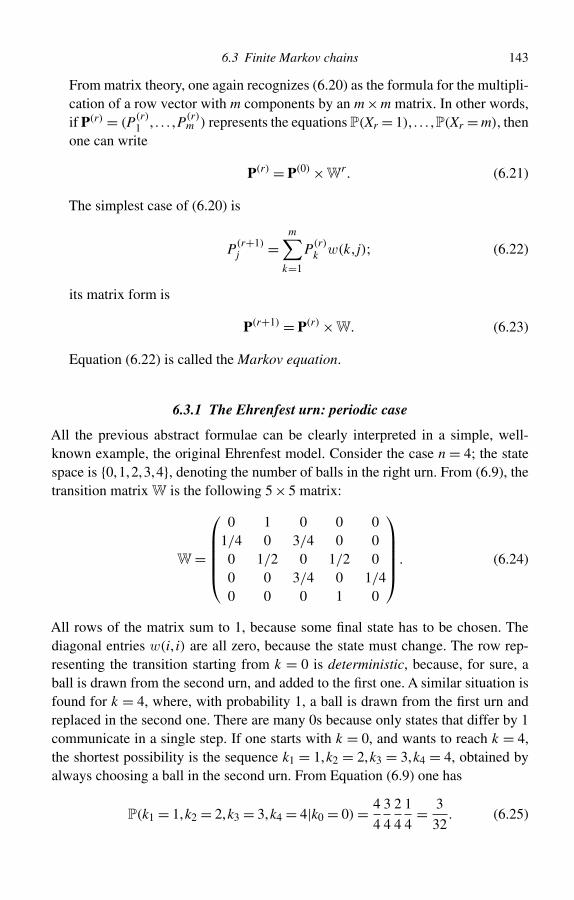
6.3 Finite Markov chains 143
From matrix theory, one again recognizes (6.20) as the formula for the multipli-cation of a row vector with m components by an m × m matrix. In other words,if P(r) = (P(r)
1 , . . . ,P(r)m ) represents the equations P(Xr = 1), . . . ,P(Xr = m), then
one can write
P(r) = P(0) ×Wr . (6.21)
The simplest case of (6.20) is
P(r+1)j =
m∑k=1
P(r)k w(k, j); (6.22)
its matrix form is
P(r+1) = P(r) ×W. (6.23)
Equation (6.22) is called the Markov equation.
6.3.1 The Ehrenfest urn: periodic case
All the previous abstract formulae can be clearly interpreted in a simple, well-known example, the original Ehrenfest model. Consider the case n = 4; the statespace is {0,1,2,3,4}, denoting the number of balls in the right urn. From (6.9), thetransition matrix W is the following 5 × 5 matrix:
W =
0 1 0 0 0
1/4 0 3/4 0 00 1/2 0 1/2 00 0 3/4 0 1/40 0 0 1 0
. (6.24)
All rows of the matrix sum to 1, because some final state has to be chosen. Thediagonal entries w(i, i) are all zero, because the state must change. The row rep-resenting the transition starting from k = 0 is deterministic, because, for sure, aball is drawn from the second urn, and added to the first one. A similar situation isfound for k = 4, where, with probability 1, a ball is drawn from the first urn andreplaced in the second one. There are many 0s because only states that differ by 1communicate in a single step. If one starts with k = 0, and wants to reach k = 4,the shortest possibility is the sequence k1 = 1,k2 = 2,k3 = 3,k4 = 4, obtained byalways choosing a ball in the second urn. From Equation (6.9) one has
P(k1 = 1,k2 = 2,k3 = 3,k4 = 4|k0 = 0) = 4
4
3
4
2
4
1
4= 3
32. (6.25)
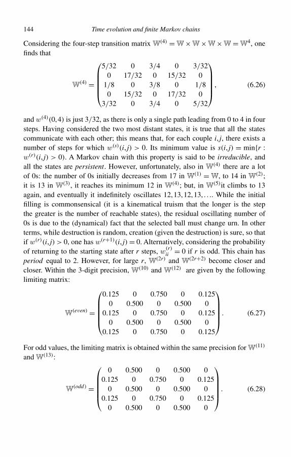
144 Time evolution and finite Markov chains
Considering the four-step transition matrix W(4) = W × W × W × W = W4, onefinds that
W(4) =
5/32 0 3/4 0 3/32
0 17/32 0 15/32 01/8 0 3/8 0 1/80 15/32 0 17/32 0
3/32 0 3/4 0 5/32
, (6.26)
and w(4)(0,4) is just 3/32, as there is only a single path leading from 0 to 4 in foursteps. Having considered the two most distant states, it is true that all the statescommunicate with each other; this means that, for each couple i, j, there exists anumber of steps for which w(s)(i, j) > 0. Its minimum value is s(i, j) = min{r :w(r)(i, j) > 0). A Markov chain with this property is said to be irreducible, andall the states are persistent. However, unfortunately, also in W(4) there are a lotof 0s: the number of 0s initially decreases from 17 in W(1) = W, to 14 in W(2);it is 13 in W(3), it reaches its minimum 12 in W(4); but, in W(5)it climbs to 13again, and eventually it indefinitely oscillates 12,13,12,13, . . .. While the initialfilling is commonsensical (it is a kinematical truism that the longer is the stepthe greater is the number of reachable states), the residual oscillating number of0s is due to the (dynamical) fact that the selected ball must change urn. In otherterms, while destruction is random, creation (given the destruction) is sure, so thatif w(r)(i, j) > 0, one has w(r+1)(i, j) = 0. Alternatively, considering the probabilityof returning to the starting state after r steps, w
(r)ii = 0 if r is odd. This chain has
period equal to 2. However, for large r, W(2r) and W(2r+2) become closer andcloser. Within the 3-digit precision, W(10) and W(12) are given by the followinglimiting matrix:
W(even) =
0.125 0 0.750 0 0.125
0 0.500 0 0.500 00.125 0 0.750 0 0.125
0 0.500 0 0.500 00.125 0 0.750 0 0.125
. (6.27)
For odd values, the limiting matrix is obtained within the same precision for W(11)
and W(13):
W(odd) =
0 0.500 0 0.500 0
0.125 0 0.750 0 0.1250 0.500 0 0.500 0
0.125 0 0.750 0 0.1250 0.500 0 0.500 0
. (6.28)
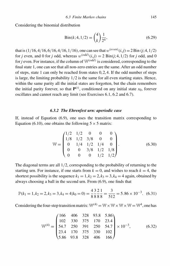
6.3 Finite Markov chains 145
Considering the binomial distribution
Bin(k;4,1/2) =(
4
k
)1
24, (6.29)
that is (1/16,4/16,6/16,4/16,1/16), one can see that w(even)(i, j)=2 Bin (j;4,1/2)
for j even, and 0 for j odd, whereas w(odd)(i, j) = 2 Bin(j;4,1/2) for j odd, and 0for j even. For instance, if the column of W(odd) is considered, corresponding to thefinal state 1, one can see that all non-zero entries are the same. After an odd numberof steps, state 1 can only be reached from states 0,2,4. If the odd number of stepsis large, the limiting probability 1/2 is the same for all even starting states. Hence,within the same parity all the initial states are forgotten, but the chain remembersthe initial parity forever, so that P(t), conditioned on any initial state x0, foreveroscillates and cannot reach any limit (see Exercises 6.1, 6.2 and 6.7).
6.3.2 The Ehrenfest urn: aperiodic case
If, instead of Equation (6.9), one uses the transition matrix corresponding toEquation (6.10), one obtains the following 5 × 5 matrix:
W =
1/2 1/2 0 0 01/8 1/2 3/8 0 00 1/4 1/2 1/4 00 0 3/8 1/2 1/80 0 0 1/2 1/2
. (6.30)
The diagonal terms are all 1/2, corresponding to the probability of returning to thestarting urn. For instance, if one starts from k = 0, and wishes to reach k = 4, theshortest possibility is the sequence k1 = 1,k2 = 2,k3 = 3,k4 = 4 again, obtained byalways choosing a ball in the second urn. From (6.9), one finds that
P(k1 = 1,k2 = 2,k3 = 3,k4 = 4|k0 = 0) = 4
8
3
8
2
8
1
8= 3
512= 5.86 × 10⁻³. (6.31)
Considering the four-step transition matrix: W(4) =W×W×W×W=W4, one has
W(4) =
166 406 328 93.8 5.86102 330 375 170 23.454.7 250 391 250 54.723.4 170 375 330 1025.86 93.8 328 406 166
× 10−3, (6.32)
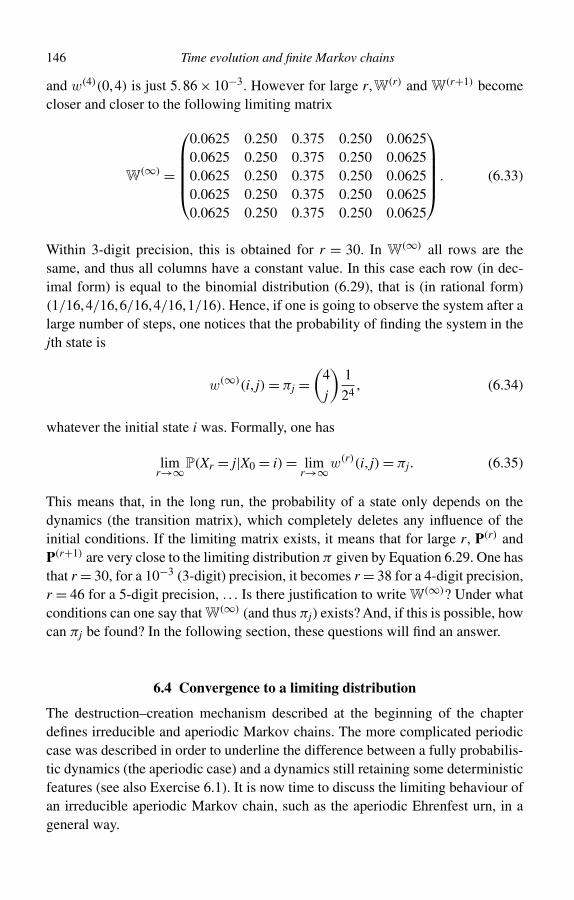
146 Time evolution and finite Markov chains
and w(4)(0,4) is just 5.86 × 10⁻³. However for large r,W(r) and W(r+1) becomecloser and closer to the following limiting matrix
W(∞) =
0.0625 0.250 0.375 0.250 0.06250.0625 0.250 0.375 0.250 0.06250.0625 0.250 0.375 0.250 0.06250.0625 0.250 0.375 0.250 0.06250.0625 0.250 0.375 0.250 0.0625
. (6.33)
Within 3-digit precision, this is obtained for r = 30. In W(∞) all rows are thesame, and thus all columns have a constant value. In this case each row (in dec-imal form) is equal to the binomial distribution (6.29), that is (in rational form)(1/16,4/16,6/16,4/16,1/16). Hence, if one is going to observe the system after alarge number of steps, one notices that the probability of finding the system in thejth state is
w(∞)(i, j) = πj =(
4
j
)1
24, (6.34)
whatever the initial state i was. Formally, one has
limr→∞P(Xr = j|X0 = i) = lim
r→∞w(r)(i, j) = πj. (6.35)
This means that, in the long run, the probability of a state only depends on thedynamics (the transition matrix), which completely deletes any influence of theinitial conditions. If the limiting matrix exists, it means that for large r, P(r) andP(r+1) are very close to the limiting distribution π given by Equation 6.29. One hasthat r = 30, for a 10−3 (3-digit) precision, it becomes r = 38 for a 4-digit precision,r = 46 for a 5-digit precision, . . . Is there justification to write W(∞)? Under whatconditions can one say that W(∞) (and thus πj) exists? And, if this is possible, howcan πj be found? In the following section, these questions will find an answer.
6.4 Convergence to a limiting distribution
The destruction–creation mechanism described at the beginning of the chapterdefines irreducible and aperiodic Markov chains. The more complicated periodiccase was described in order to underline the difference between a fully probabilis-tic dynamics (the aperiodic case) and a dynamics still retaining some deterministicfeatures (see also Exercise 6.1). It is now time to discuss the limiting behaviour ofan irreducible aperiodic Markov chain, such as the aperiodic Ehrenfest urn, in ageneral way.
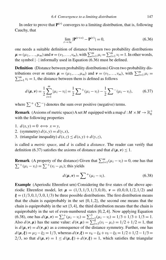
6.4 Convergence to a limiting distribution 147
In order to prove that P(r) converges to a limiting distribution, that is, followingCauchy, that
limr→∞|P(r+s) − P(r)| = 0, (6.36)
one needs a suitable definition of distance between two probability distributionsµ= (µ1, . . . ,µm) and ν = (ν1, . . . ,νm), with
∑mi=1 µi =∑m
i=1 νi = 1. In other words,the symbol | · | informally used in Equation (6.36) must be defined.
Definition (Distance between probability distributions) Given two probability dis-tributions over m states µ = (µ1, . . . ,µm) and ν = (ν1, . . . ,νm), with
∑mi=1 µi =∑m
i=1 νi = 1, the distance between them is defined as follows
d(µ,ν) = 1
2
m∑i=1
|µi − νi| = 1
2
∑+(µi − νi)− 1
2
∑−(µi − νi), (6.37)
where∑+ (
∑−) denotes the sum over positive (negative) terms.
Remark (Axioms of metric space) A set M equipped with a map d : M ×M → R+0
with the following properties
1. d(x,y) = 0 ⇐⇒ x = y,2. (symmetry) d(x,y) = d(y,x),3. (triangular inequality) d(x,z) ≤ d(x,y)+ d(y,z),
is called a metric space, and d is called a distance. The reader can verify thatdefinition (6.37) satisfies the axioms of distance and that d(µ,ν) ≤ 1.
Remark (A property of the distance) Given that∑m
i=1(µi − νi) = 0, one has that∑+(µi − νi) =∑+(νi −µi); this yields
d(µ,ν) =∑+(µi − νi). (6.38)
Example (Aperiodic Ehrenfest urn) Considering the five states of the above ape-riodic Ehrenfest model, let µ = (1/3,1/3,1/3,0,0), ν = (0,0,0,1/2,1/2) andξ = (1/3,0,1/3,0,1/3) be three possible distributions. The first distribution meansthat the chain is equiprobably in the set {0,1,2}, the second one means that thechain is equiprobably in the set {3,4}, the third distribution means that the chain isequiprobably in the set of even-numbered states {0,2,4}. Now applying Equation(6.38), one has d(µ,ν) =∑+
i (µi − νi) =∑3i=1(µi − νi) = 1/3 + 1/3 + 1/3 = 1.
Also d(ν,µ) has the same value: d(ν,µ) =∑4i=3(νi − µi) = 1/2 + 1/2 = 1, that
is d(µ,ν) = d(ν,µ) as a consequence of the distance symmetry. Further, one hasd(µ,ξ) = µ2 −ξ2 = 1/3, whereas d(ν,ξ) = ν4 −ξ4 +ν5 −ξ5 = 1/2+1/2−1/3 =2/3, so that d(µ,ν) = 1 ≤ d(µ,ξ) + d(ν,ξ) = 1, which satisfies the triangular
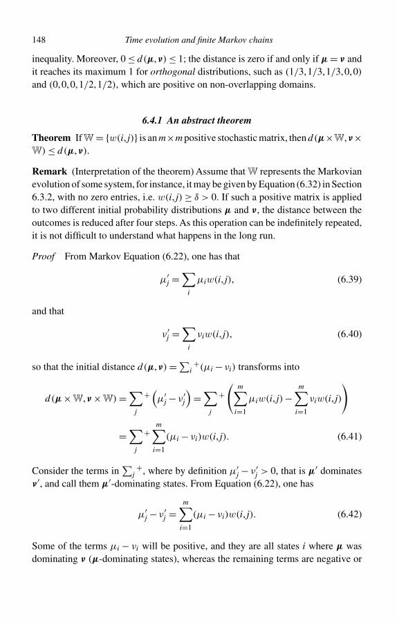
148 Time evolution and finite Markov chains
inequality. Moreover, 0 ≤ d(µ,ν) ≤ 1; the distance is zero if and only if µ = ν andit reaches its maximum 1 for orthogonal distributions, such as (1/3,1/3,1/3,0,0)
and (0,0,0,1/2,1/2), which are positive on non-overlapping domains.
6.4.1 An abstract theorem
Theorem If W = {w(i, j)} is an m×m positive stochastic matrix, then d(µ×W,ν×W) ≤ d(µ,ν).
Remark (Interpretation of the theorem) Assume that W represents the Markovianevolution of some system, for instance, it may be given by Equation (6.32) in Section6.3.2, with no zero entries, i.e. w(i, j) ≥ δ > 0. If such a positive matrix is appliedto two different initial probability distributions µ and ν, the distance between theoutcomes is reduced after four steps. As this operation can be indefinitely repeated,it is not difficult to understand what happens in the long run.
Proof From Markov Equation (6.22), one has that
µ′j =∑
i
µiw(i, j), (6.39)
and that
ν′j =∑
i
νiw(i, j), (6.40)
so that the initial distance d(µ,ν) =∑i+(µi − νi) transforms into
d(µ×W,ν ×W) =∑
j
+(µ′j − ν′
j
)=∑
j
+(
m∑i=1
µiw(i, j)−m∑
i=1
νiw(i, j)
)
=∑
j
+m∑
i=1
(µi − νi)w(i, j). (6.41)
Consider the terms in∑
j+, where by definition µ′
j − ν′j > 0, that is µ′ dominates
ν′, and call them µ′-dominating states. From Equation (6.22), one has
µ′j − ν′
j =m∑
i=1
(µi − νi)w(i, j). (6.42)
Some of the terms µi − νi will be positive, and they are all states i where µ wasdominating ν (µ-dominating states), whereas the remaining terms are negative or
6.4 Convergence to a limiting distribution 149
vanish. Therefore, one further has
µ′j − ν′
j =m∑
i=1
(µi − νi)w(i, j) ≤∑
i
+(µi − νi)w(i, j). (6.43)
Each term of∑+
i denotes the fraction of the µ-dominance which is transferred toa µ′-dominating state. Then summing on all µ′-dominating states, one arrives at∑
j
+(µ′j − ν′
j) ≤∑
j
+∑i
+(µi − νi)w(i, j). (6.44)
Inverting the summation order, one finds that the term∑i
+(µi − νi)∑
j
+w(i, j) (6.45)
takes into account how each ‘piece’ of the old distance µi −νi > 0 is transferred tothe new µ′-dominating states. Therefore, one gets that
d(µ×W,ν ×W) ≤∑
i
+(µi − νi)∑
j
+w(i, j) ≤∑
i
+(µi − νi)
m∑j=1
w(i, j)
=∑
i
+(µi − νi) = d(µ,ν). (6.46)
Given that∑
j+w(i, j) differs from
∑mj=1 w(i, j) = 1 in at least one term, one has
that∑
j+w(i, j) ≤ 1 − δ, and thus
d(µ×W,ν ×W) ≤ (1 − δ)d(µ,ν), (6.47)
with δ = mini,j(w(i, j)). �
Remark (Conceptual core) This is the conceptual core of the previous theorem:Markov evolution mixes all the states, so that, if some µ-dominance is present atthe beginning, given that all w(i, j) are positive, the quantity
∑i+(µi −νi) diffuses
not only towards µ′-dominated states, but also towards ν′-dominated states, andthus the dominating mass is reduced.
6.4.2 Applications to finite Markov chains
Considering the seven dice chain, or the aperiodic Ehrenfest model, W(n) is apositive stochastic matrix, where in general n stands for the size of the population(of dice, or of balls). Intuitively, after n steps all the states have positive probabilityof being reached from any initial state. The transition matrix for the dice chain
150 Time evolution and finite Markov chains
is 792 × 792 and it was not explicitly written, but from Equation (6.6) one cansee that P(Yt+1 = n|Yt = n) = 1/6 > 0 implies no periodicity at all. The periodiccase is different, where for no r, it is true that W(r) is positive. The rest of thebook is devoted to irreducible aperiodic chains of the kind described in Section6.1.4, for which there always exists an r such that W(r) is positive (an alternativedefinition is: W is regular if W(r) is positive for some r). If W(r) is positive, alsoW(r+1) = W × W(r) is positive. Moreover, if W(r) is positive, also P(r) = P(0)×W(r) is positive for all states, whatever P(0) may be.
Theorem (Main theorem for irreducible aperiodic Markov chains (Sinai)) For anyirreducible aperiodic Markov chain, that is a Markov chain whose transition matrixis regular, there exists a unique probability distribution π = (π1, . . . ,πm), πj > 0,such that:
1. πj is the long-term limit of the probability P(Xr = j) = P(r)j :
πj = limr→∞P(Xr = j); (6.48)
2. π is the (unique) invariant distribution of the chain, meaning that
π ×W = π ; (6.49)
3. πj is the long-term limit of the rows of the r-step transition matrix:
limr→∞w(r)(i, j) = πj. (6.50)
Proof For concrete systems governed by a regular transition matrix, one canconsider P(0),P(1) = P(0)× W, . . . ,P(n) = P(0)× W(n), and show that the sequence{P(n)}n∈N is a Cauchy one, meaning that
limn→∞d(P(n),P(n+p)) = 0. (6.51)
This equation clarifies the meaning of Equation (6.36). Now P(n) and P(n+p) standfor µ and ν in the theorem discussed above. The matrix being regular, assume thatW(r) is positive; it plays the role of W in the previous theorem. As a consequenceof Equations (6.21) and (6.47), one can write
d(P(n−r) ×W(r),P(n+p−r) ×W(r)) ≤ (1 − δ)d(P(n−r),P(n+p−r)), (6.52)
where δ = mini,j(w(r)(i, j)); in other words, the time evolution reduces the distance
with respect to r steps before. This consideration can be iterated, leading to
d(P(n),P(n+p)) ≤ (1 − δ)2d(P(n−2r),P(n+p−2r)), (6.53)
6.4 Convergence to a limiting distribution 151
and so on. If n = mr + s, s = 1,2, . . . ,m − 1, then one finds
d(P(n),P(n+p)) ≤ (1 − δ)md(P(n−mr),P(n+p−mr)) ≤ (1 − δ)m, (6.54)
as one always has that d(µ,ν) < 1. Hence, for any ε > 0 there is an n large enoughso that (1 − δ)m < ε for some m. Therefore, the sequence {P(n)}n∈N is a Cauchysequence and the limit
limr→∞P(r) = π , (6.55)
exists;1 in other words, the mixing property of the transition matrix produces alimiting distribution in the long run.
With Equation (6.55) point 1 of the theorem is proven. Now, consider thefollowing chain of equalities
π ×W = limt→∞P(t) ×W = lim
t→∞P(0) ×W(t) ×W = limt→∞P(0) ×W(t+1) = π ;
(6.56)
this means that
π ×W =π , (6.57)
which proves one part of point 2. A probability distribution satisfiying Equation(6.57) is said to be an invariant distribution of the chain. Therefore, the limitingdistribution is just the invariant distribution of the chain. That π is unique is givenby the fact that, if π and π ′ are both invariant, they do not change by multiplicationby W(r); hence, as a consequence of the abstract theorem d(π ×W(r),π ′ ×W(r)) =d(π ,π ′) ≤ (1−δ)d(π ,π ′), then d(π ,π ′) = 0, and as a consequence of the distanceproperties, one eventually gets π = π ′. This proves the uniqueness of the invariantdistribution in the case under scrutiny and completes the proof of point 2.
It is often useful and instructive to consider the initial distribution as degenerate,or deterministic, that is P(0) = (0, . . . ,0,1,0, . . . ,0) = δ(x − x0), in order to observehow the probability mass spreads as a consequence of the Markov dynamics. Themass is initially concentrated on a single state, then diffuses on all the availablestates as time goes by. In this case, one can write
P(r) = P(0) ×W(r) = w(r)(i, j), (6.58)
1 Strictly speaking, one needs the completeness for the metric space of probability distributions on m states.Completeness means that every Cauchy distribution has a limit. This is true if the distributions are real valued.
152 Time evolution and finite Markov chains
where i is the index of the only initial state. Therefore, as a consequence of Equation(6.55), one immediately has that
limr→∞w(r)(i, j) = πj; (6.59)
this shows that the equilibrium distribution does not depend on the initial one (thereis a complete memory loss) and completes the proof of point 3 and of the theorem.
�
Remark (Speed of convergence) Regarding the speed of convergence of P(0) =δ(x−x0) to π , the following considerations are possible. Given that π = π ×W(n),and d(P(n),π) = d(P(0) ×W(n),π ×W(n)) ≤ . . . ≤ (1−δ)m, where m is the integerpart of n/r, one knows that the distance diminishes each r steps, but one desiresa formula containing any step n. Now, assume that r = 4, as in the example ofSection 6.3.2, then one has d(P(31),π) ≤ (1− δ)7 as 31 = 7 ·4+3, and 7 ≥ 31/4−1 = 6.75. As a function of n, m + 1 is 1 for n = 1,2,3; it is 2 for n = 4,5,6,7.Therefore m ≥ (n/r) − 1 and given that (1 − δ) < 1, it increases if the exponentdecreases. Then (1 − δ)m ≤ (1 − δ)(n/r)−1 = (1 − δ)−1(1 − δ)n/r = (1 − δ)−1γ n,where γ = (1 − δ)1/r < 1. Finally, one finds
d(P(n),π) ≤ (1 − δ)−1γ n, (6.60)
and the speed of convergence is exponential, or it is faster than any power of n. SeeExercise 6.3 for further details.
6.5 The invariant distribution
6.5.1 On the existence of the invariant distribution
The invariant distribution exists (and is unique) not only for any regular (irre-ducible and aperiodic) Markov chain, but also in the irreducible and periodic case.For regular chains, it is also the equilibrium distribution, that is limr→∞ P(Xr =j|X0 = x0) = πj for any initial state x0. This is not possible for periodic chains,where the parity of the initial state is there forever. However, if there exists a prob-ability distribution on all the m states π satisfying the Markov Equation (6.22),one can conclude that, given that P(r) = π , also P(r+1) = π × W =π , and thisis true for all the future steps. For the aperiodic case this would be an artifi-cial way to prepare the initial state: if the initial state is such that P(0) = π ,then the Markov chain would be a stationary process (see Exercise 6.1). Inorder to find the invariant distribution π , one should check if the set of m
6.5 The invariant distribution 153
linear equations π1 =∑m
i=1 πiw(i,1),. . .
πj =∑mi=1 πiw(i, j),. . .
πm =∑mi=1 πiw(i,m) (6.61)
has a solution for πj > 0, with∑m
i=1 πj = 1. In matrix terms, it is the solutionof the equation π = π × W, where π is the left eigenvector of W correspondingto the eigenvalue 1. In very simple examples (see the exercises), this route canbe followed, but in our applications to physical and economic systems the statespace is very large, and the search for the invariant distribution will follow anothermethod. Regarding the meaning of Equation (6.61), writing the Markov equationexplicitly for the jth state, one has that
P(Xs+1 = j) =m∑
i=1
P(Xs = i)w(i, j) (6.62)
decribes the decomposition of the probability mass for the jth state at step s+1 as asum of all contributions at the previous step. If there exists a distribution P(Xs = i),i = 1, . . . ,m, such that the ‘traffic’ w(i, j) leaves it invariant, π is found. This is justa mathematical property, and nothing is said about the fact that a specific system,prepared in some state, will sooner or later be described by π .
In order to prove the existence of the invariant distribution, one can simply con-sider an irreducible Markov chain described by the one-step transition probabilitymatrix W and by the initial probability distribution P(0). As mentioned above, thehypothesis of aperiodicity is not necessary. For instance, if P(0) has all its mass onx0, P(1) will be positive on the nearest neighbours of x0 (the states with which x0
communicates), and, as time goes by, all entries of P(s) will become positive (ifthe matrix is regular, that is the chain is aperiodic), or they will have an oscillatorypresence of zero and positive entries, if the matrix is periodic. What would happenif one uses this abstract mean:
P(0)
(s) = 1
s
s−1∑r=0
P(r) = 1
s{P(0) + . . .+ P(s−1)} (6.63)
as initial probability? This is the time average of the first s probability distributionson the states. An intuitive meaning of this distribution is given below. However, atthe second step, from Markov Equation (6.22), one gets
P(1)
(s) = P(0)
(s)×W =1
s{P(1) + . . .+ P(s)}, (6.64)
154 Time evolution and finite Markov chains
so that
P(1)
(s)− P(0)
(s) = 1
s{P(s) − P(0)}, (6.65)
and
|P(1)(s)− P
(0)(s)| = 1
s|P(s) − P(0)| ≤ 2
s. (6.66)
This difference can be made as small as desired, provided that s → ∞. In other
words, lims→∞ P(0)
(s) does not vary during the time evolution. Therefore, theinvariant distribution
π = lims→∞
1
s{P(1) + . . .+ P(s)} (6.67)
does exist for periodic chains also.Now, consider the periodic Ehrenfest urn; if w(r)(i, j) is positive, then w(r+1)(i, j)
is zero, and, for large s, if r is even, w(r)(i, j) w(even)(i, j), while w(r+1)(i, j) w(odd)(i, j). Moreover, introducing the limiting matrix of the aperiodic case,
w(∞)(i, j) = 1
2(w(odd)(i, j)+w(even)(i, j)), (6.68)
and given that one of them is zero, either w(odd)(i, j) is 0 or it is equal to 2w(∞)ij ,
and the same is true for w(even).Assume that one considers a periodic and an aperiodic chain with the same space
state and both starting from the same initial state, say x0 = 0, and focus on the jthstate. Consider
Pj(0)
(s) = 1
s{P(0)
j + . . .+ P(s−1)j }. (6.69)
If j �= 0, then one starts with P(0)j = 0, but, after some steps, this probability will
be positive, as all states communicate with each other in both cases (both chainsare assumed to be irreducible). Note that starting with x0 = 0 amounts to settingP(t)
j = w(t)(0, j). Omitting the initial steps, whose weight goes to zero if s is large,
and considering two consecutive steps, in the aperiodic case, both w(t)(0, j) andw(t+1)(0, j) are positive and converge to w(∞)(0, j), whereas only one of them ispositive in the periodic case, but the positive term converges to 2w(∞)(0, j). Thenin the sum
1
s{P(0)
j + . . .+ P(s−1)j }, (6.70)
the correlation between time and values is lost, and the invariant distribution existsfor both the aperiodic and the periodic case.
6.5 The invariant distribution 155
6.5.2 The frequency meaning of the invariant distribution
An intuitive meaning of the invariant distribution is as follows. One is interestedin the time-fraction in which the system visits any given state as time goes by. Asusual (see Section 4.1.8), one can define I (r)
j as the indicator function I{Xr=j} of theevent Xr = j. Therefore the random variable
Jj,s = 1
s
s−1∑r=0
I (r)j (6.71)
denotes the relative frequency of visits to the state j after s steps. The expectedvalue of I (r)
j is
E(I (r)j ) = P(Xr = j) = P(r)
j . (6.72)
Therefore,
E(Jj,s) = 1
s
s−1∑r=0
E(I (r)j ) = 1
s{P(0)
j + . . .+ P(s−1)j } (6.73)
is just the expected relative frequency of visits to the jth state after s steps. Ifthere exists
πj = lims→∞
1
s{P(0)
j + . . .+ P(s−1)j }, (6.74)
then the expected relative frequency of visits is such that
lims→∞E(Jj,s) = πj. (6.75)
This link between a probability value πj (which is a measure) and the relativefrequency Jj,s (that is a random variable) can be made stronger by also consideringthe variance of Jj,s. Indeed, it is possible to prove that
√V(Jj,s)/E(Jj,s) vanishes
for large s, and this is the basis of the (weak) law of large numbers for irreducibleMarkov chains and the consequent ergodic theorem.
6.5.3 The law of large numbers for irreducible Markov chains
From Exercise 5.2, the variance of the sum of s random variables is given by
V
(s∑
i=1
Xi
)=
s∑i=1
V(Xi)+ 2s∑
i=1
s∑j=i+1
C(Xi,Xj), (6.76)
156 Time evolution and finite Markov chains
a formula consisting of s diagonal terms and s(s − 1) out-of-diagonal terms for agrand-total of s2 terms.
If the random variables Xi were independent (or uncorrelated), one would haveC(Xi,Xj) = 0, and only s terms would survive in Equation (6.76); if they wereexchangeable, then C(Xi,Xj) would not depend on i, j and they would be positive;as a consequence, all the s2 terms would be positive. When one is interested in thevariance of
∑si=1 Xi/s, one must divide Equation (6.76) by s2 and this is the rea-
son the variance of∑s
i=1 Xi/s vanishes for independent variables (self-averaging),and does not vanish for exchangeable variables (lack of self-averaging). In theMarkovian case, correlations decrease as a function of |j − i|, so that the varianceof∑s
i=1 Xi/s vanishes for s → ∞.Now, consider the variance of Jj,s defined in Equation (6.71). The following
calculations are valid only for an aperiodic irreducible Markov chain, but the resultcan be extended to the periodic case. Following Penrose [1], one has
V(Jj,s) = 1
s2V
(s∑
r=1
I (r)j
), (6.77)
and
V
(s∑
r=1
I (r)j
)=
s∑r=1
V(I (r)j )+
s∑r=1
s∑u=r+1
C(I (r)j , I (u)
j )
+s∑
r=1
r−1∑u=1
C(I (r)j , I (u)
j ) = v1 + v2 + v3, (6.78)
where the out-of-diagonal terms are divided into future (u > r) and past (u < r)covariances. Regarding v1 one finds that (see Exercise 4.4)
V(I (r)j ) = P(r)
j [1 − P(r)j ] ≤ 1/4; (6.79)
therefore,
v1 ≤ s/4. (6.80)
Regarding v2, one can use the result of Exercise 5.3 to find that
C(I (r)j , I (u)
j ) = P(Xr = j,Xu = j)−P(Xr = j)P(Xu = j)
= P(r)j [w(u−r)(j, j)− P(u)
j ], (6.81)
6.5 The invariant distribution 157
which is the covariance of the rth variable and the uth, with r < u ≤ s, distant u− rsteps. Further,
v2 =s∑
r=1
s∑u=r+1
P(r)j [w(u−r)(j, j)− P(u)
j ] =s∑
r=1
P(r)j
s∑u=r+1
[w(u−r)(j, j)− P(u)j ].
(6.82)
The correlation C(I (r)j , I (u)
j ) can also be negative; therefore, given that P(r)j ≤ 1,
|v2| ≤s∑
r=1
s∑u=r+1
|w(u−r)(j, j)− P(u)j |. (6.83)
Note that
|w(u−r)(j, j)− P(u)j | ≤ |w(u−r)(j, j)−πj|+ |πj − P(u)
j |, (6.84)
and both w(u−r)(j, j) and P(u)j converge to πj for large u and u− r. Therefore, when
s is large, most of the s(s − 1)/2 terms in the double sum will vanish. Eventually,using the inequality in (6.84), one finds
|v2| ≤s∑
r=1
s∑u=r+1
|w(u−r)(j, j)−πj|+s∑
r=1
s∑u=r+1
|πj − P(u)j |. (6.85)
For any r, the first summand on the right-hand side of inequality (6.85) sums s − rterms |w(u−r)(j, j)−πj| = |w(t)(j, j)−πj|, where t = u − r varies in 1, . . . ,s − r. Ifone also adds the remaining r terms, a new upper bound is obtained:
s∑r=1
s∑u=r+1
|w(u−r)(j, j)−πj| =s∑
r=1
s−r∑t=1
|w(t)(j, j)−πj|
≤s∑
r=1
s∑t=1
|w(t)(j, j)−πj| = ss∑
t=1
|w(t)(j, j)−πj|, (6.86)
as the first sum does not depend on r. Symmetrically adding r terms in the secondsummand, the final new upper bound for v2 is
|v2| ≤ ss∑
t=1
[|w(t)(j, j)−πj|+ |πj − P(t)j |]. (6.87)
158 Time evolution and finite Markov chains
From the limiting properties of w(t)(j, j) and P(t)j , it turns out that for any ε > 0
there exists a k such that for t > k one has2
|w(t)jj −πj|+ |πj − P(t)
j | < ε. (6.88)
But in Equation (6.87) all values of t between 1 and s are present, also small values,for which w(t)(j, j) and P(t)
j can be very different from πj. However, the sum inEquation (6.87) can be split into two parts
|v2|s
≤k∑
t=1
[|w(t)(j, j)−πj|+ |πj − P(t)j |]+
s∑t=k+1
[|w(t)(j, j)−πj|+ |πj − P(t)j |].
(6.89)
In the first part, each summand is not greater than 2, whereas, in the second, eachterm is not greater than ε; it follows that
|v2| ≤ sk∑
t=1
2 + ss∑
t=k+1
ε ≤ 2sk + s2ε. (6.90)
Returning to the variance of the relative frequency of visit, this is given by
V(Jj,s) = 1
s2(v1 + v2 + v3), (6.91)
where v3 = v2 and
|V(Jj,s)| ≤( |v1|
s2+ 2
|v2|s2
). (6.92)
From Equation (6.80), it is immediately apparent that
lims→∞
|v1|s2
= lims→∞
v1
s2≤ lim
s→∞1
4s= 0. (6.93)
To show that also
lims→∞
|v2|s2
= 0, (6.94)
it is sufficient to note that, from Equation (6.90), one has
|v2|s2
≤ 2k
s+ ε. (6.95)
2 It is assumed that s is large enough, as one is interested in s → ∞.
6.5 The invariant distribution 159
Then, if s ≥ 2k/ε in addition to s ≥ k, one gets
|v2|s2
≤ 2k
s+ ε ≤ ε + ε = 2ε, (6.96)
which suffices to prove (6.94). Therefore, from Equation (6.92), one finds that
lims→∞V(Jj,s) = 0. (6.97)
In order to see this more clearly, consider the previous aperiodic model, settingj = 0 and P(0)
0 = 1, P(0) = (1,0,0,0,0), in which case w(t)(j, j) = P(t)j ; if one chooses
ε = 0.01, then one finds that |w(t)(j, j)−πj|+ |πj −P(t)j | = 2|w(t)(j, j)−πj| < 0.01
for t = k > 14. Writing down the upper limit, one finds that |v2|/s2 ≤ 28/s + 0.01.If one requires that |v2|/s2 ≤ 2ε, one needs 28/s < 0.01, that is s > 2800.
Using the Bienaymé–Chebyshev inequality (see Exercise 6.4),
P(|Jj,s −E(Jj,s)| ≥ δ) ≤ V(Jj,s)
δ2, (6.98)
and recalling Equation (6.75) yields
lims→∞P(|Jj,s −πj| ≥ δ) = 0. (6.99)
This is the weak law of large numbers for irreducible Markov chains, stating that,given a difference δ > 0 between the observed relative frequency Ji,s and the valueπi, there exists ε > 0 and a number of steps s(δ,ε) such that the probability of exceed-ing δ is less than ε. Considering all states together, the vector Js = (J1,s, . . . ,Jm,s),with
∑mi=1 Ji,s = 1, represents the normalized histogram of the relative visiting fre-
quencies after s steps. One expects that lims→∞ d(Js,π) → 0. If one considers afunction X of the state i such that X (i) = xi, then X can be decomposed in normalform, that is
Xt =n∑
i=1
xiI(t)i . (6.100)
Its time average is the random variable
X s = 1
s
s∑t=1
Xt = 1
s
s∑t=1
m∑i=1
xiI(t)i = 1
s
m∑i=1
xi
s∑t=1
I (t)i =
m∑i=1
xiJi,s, (6.101)
where the sum on steps was transformed into a sum on values weighted by theirrelative frequency. Due to the fact that d(Js,π) → 0 for s → ∞, one expects that
160 Time evolution and finite Markov chains
X s =∑mi=1 xiJi,s will converge to
Eπ (X ) =m∑
i=1
xiπi. (6.102)
This is stronger than claiming that, for s → ∞, one has E(X s) → Eπ (X ). Thisproperty means that, repeating many times i = 1, . . . ,n a very long sequence
X (i)0 ,X (i)
1 , . . . ,X (i)s , the time averages X
(i)s are distributed around Eπ (X ). The (weak)
ergodic theorem states that
lims→∞P(|X s −Eπ (X )| ≥ δ) = 0. (6.103)
Equation (6.103) means that X s converges to its limiting expectation value Eπ (X )
with a variance which is vanishing for large s. This theorem will not be provedhere. As a final remark, note that equations such as (6.99) and (6.103) lie at thefoundation of the Markov chain Monte Carlo simulation method which will beused in the following sections.
6.6 Reversibility
Is there any property which allows an exact evaluation of the invariant distributionπ? In order to answer this question, consider the Markov equation once more,
P(Xs+1 = j) =m∑
i=1
P(Xs = i)w(i, j), (6.104)
and given that
m∑i=1
w(j, i) = 1, (6.105)
one finds
P(Xs = j) =m∑
i=1
P(Xs = j)w(j, i). (6.106)
Subtracting this equation from Equation (6.104), one gets the so-called discretemaster equation
P(Xs+1 = j)−P(Xs = j) =m∑
i=1
[P(Xs = i)w(i, j)−P(Xs = j)w(j, i)] . (6.107)
6.6 Reversibility 161
Equation (6.107) can be written in a shorter form, omitting the term i = j, whichvanishes
P(s+1)j − P(s)
j =∑i �=j
[P(s)
i w(i, j)− P(s)j w(j, i)
]. (6.108)
The master equation can be understood as follows: the difference P(s)j = P(s+1)
j −P(s)
j is the increment of the probability mass for the jth state, whereas P(s)i w(i, j)−
P(s)j w(j, i) is the net traffic (the net flux) along the road connecting the states i and
j. Note that P(s)i w(i, j) is the ith state mass flux entering the state j, and P(s)
j w(j, i) isjth state mass flux leaving towards state i. If, for any couple i, j, the total flux is zero
P(s)i w(i, j) = P(s)
j w(j, i), (6.109)
then P(s+1)j = P(s)
j = πj. In other words, if a distribution satisfies the detailed bal-ance conditions (6.109), it is the invariant distribution. Note that Equation (6.109)is not a necessary condition for the invariant distribution: for any πj, the globalbalance is zero, whereas detailed balance is a property valid for each pair of states.The master equation and the balance equations may seem intuitive in the ensembleinterpretation of probability (see Exercise 6.1). In this framework, P(s)
i w(i, j) is
proportional to the number of systems passing from i to j, and P(s)j w(j, i) is propor-
tional to the number of systems passing from j to i. If they are equal for all couples,the number of systems in the jth state does not change in time.
One may wonder whether there is some simple property which can help in show-ing that the invariant distribution satisfies detailed balance. This property exists,and it is called reversibility. The intuitive meaning is the following. Consider thesequence of events S1 = . . . , it−1, jt ,kt+1, . . ., where jt is a shortcut for Xt = j, as amovie; the movie is reversible if the observer is unable to say whether the movie isbeing run forward or backward. The reversed sequence is S2 = . . . ,kt−1, jt , it+1, . . .Under what conditions can one assume that the two sequences are equiprobable? Ifso, a filmgoer could not discern whether the movie is correctly projected, or whetherit is rewinding. One can show that, if a forward movie has the scene it jt+1, thenafter a lag s > t depending on the origin of reversal, rewinding shows js−t−1is−t .Referring to the example of Section 2.4.1, the scene could be ‘agent A is a bull attime 0 and becomes a bear at time 1’. At time step 10, the movie is stopped andreversed, and for a new observer the scene at time step 10 is the initial one. Thisfilmgoer will see that ‘agent A is a bear at time 9 and passes to a bull at time 10’.
6.6.1 Backward movies
If the direct movie is a homogeneous irreducible Markov chain, what can be said ofthe reversed one? Consider the sequence S = . . . , it−1, jt ,kt+1, . . ., where, as before,
162 Time evolution and finite Markov chains
jt is a shortcut for Xt = j. Starting from a generic t, consider
P(it−1|jt ,kt+1, . . .) = P(Xt−1 = i|Xt = j,Xt+1 = k, . . .), (6.110)
which is the predictive probability of the backward movie at time step t. One canshow that:
1. the reversed predictive probability still has the Markov property, that is
P(it−1|jt ,kt+1, . . .) = P(it−1|jt). (6.111)
Indeed, it is sufficient to consider P(it−1|jt ,kt+1); from Bayes’ rule one finds:
P(it−1|jt ,kt+1) = P(it−1, jt ,kt+1)/P(jt ,kt+1). (6.112)
If the direct chain is homogeneous, then
P(it−1, jt ,kt+1)
P(jt ,kt+1)= P(it−1)w(i, j)w(j,k)
P(jt)w(j,k)= P(it−1)w(i, j)
P(jt), (6.113)
which does not depend on kt+1, and therefore the reversed process of ahomogeneous Markov chain is still a Markov chain:
P(it−1|jt ,kt+1) = P(it−1|jt) = P(it−1)w(i, j)
P(jt); (6.114)
2. from Equation (6.114), if the direct chain is stationary, that is P(it−1) = πi, andP(jt) = πj, then the reversed chain is homogeneous, and
P(it−1|jt) = u(j, i) = πiw(i, j)
πj; (6.115)
3. finally, the reversed chain has the same transition matrix as the direct chain ifand only if P(it−1|jt) = u(j, i) is equal to P(it+1|jt) = w(j, i), that is
w(j, i) = u(j, i) = πiw(i, j)
πj, (6.116)
which is again the detailed balance condition. The condition P(it−1|jt) =P(it+1|jt) expresses reversibility in the clearest way: given that Xt = j, if themovie is run forward one sees Xt+1 = i with the same probability as one seesXt−1 = i, if the movie is run backward.
The above considerations are a proof of the following
Theorem (reversible Markov chains) A homogeneous irreducible Markov chain isreversible if and only if it is stationary and the stationary distribution satisfies thedetailed balance conditions.
6.6 Reversibility 163
Concerning search of the invariant distribution, one can conclude that if the chaincannot be reversible, then one cannot make use of Equation (6.109). For instance,for a moment jump to Exercise 6.1, case a). The proposed transition matrix issuch that the state b is always followed by c; hence, reversing the movie one willalways see the opposite transition c → b, and the chain, even if stationary, is notreversible. The case of the seven dice game (in Section 6.1.4) is different: thereis no logical way to distinguish a die displaying 1 which, when cast, becomes a 4from the reversed transition, in which a 4 becomes a 1. In the case of dice, after anumber of steps sufficient to forget the initial conditions, the matrix being regular,as a consequence of Sinai’s theorem, the chain becomes closer and closer to thestationary chain, which is described by the equilibrium distribution; therefore, onecan try to see if there exists a π(n) such that:
π(n)w(n,nji) = π(nj
i)w(nji,n), j �= i (6.117)
where w(n,nji) is given by Equation (6.5). Replacing (6.5) into Equation (6.117)
and simplifying one gets
π(n)ni = π(nji)(nj + 1). (6.118)
Given that nji = (n1, . . . ,ni −1, . . . ,nj +1, . . . ,ng), and thatπ(nj
i)/π(n)= ni/(nj +1),
one finds that π(n) ∼ (∏gi=1 ni!
)−1satisfies (6.117). The normalization condition∑
n∈Sngπ(n) = 1 leads to the symmetric multinomial distribution
π(n) = n!∏gi=1 ni!
g−n, (6.119)
written for any value of n and g. This distribution is regular, that is positive forall possible n ∈ Sn
g . The same distribution describes a single experiment, where n‘fair’ dice are cast and the frequency distribution of the g = 6 results is observed.In this case, one could ask ‘what is the meaning of the number π(n)?’, and theusual discussion on the meaning of probability would start (see Chapter 1). On thecontrary, in the case of the dice game, one could record the normalized histogramof the visiting frequencies, and compare it with π(n). Distinguishing between thehistogram and π(n), by the law of large numbers for irreducible Markov chains,one can determine how long the game has to go on so that the probability that theyare closer than the fixed distance is as close to 1 as desired. Therefore, as discussedabove, the chain contains a natural ‘frequency interpretation’ of the equilibriumprobability π(n). However, this is not the only interpretation physicists give toπ(n). If an observer is going to study the system after a long time during which thesystem was left running, the limit lims→∞ P(Xs = j) = πj means that the probability
164 Time evolution and finite Markov chains
distribution to be used is P(Xs = j) = πj, whatever past information could have beenavailable. In the ‘ensemble interpretation’, πj is the fraction of (fictitious) systemswhich at time s are in state j. Further, if the observer knows that πj is also ameasure of the relative visiting frequency for state j, πj can also be considered asthe fraction of ‘favourable cases’ of finding state j over all the ‘possible cases’.Nowadays, the ‘ensemble interpretation’ can be realized in practice, by setting up alarge number of parallel computer simulations running the same Markov chain, andwith the same initial condition (and different pseudo-random number sequences).The coincidence of ensemble averages and time (or ergodic) averages is an oldproblem in ergodic theory, which finds a satisfactory solution within the frameworkof finite Markov chains.
6.6.2 Stationarity, reversibility and equilibrium
Any irreducible chain has an invariant distribution π , and, if it is aperiodic, sooneror later, it will be described by π . For an aperiodic ‘concrete’ chain, starting fromthe initial state x0, with P(0) = δ(x − x0), there will be a relaxation time duringwhich P(t) moves step-by-step towards π until the chain reaches stationarity. Asan example, consider a system where 1000 fleas are present on dog A and 0 fleason dog B. For a long initial period, it is far more likely to observe a flea fluxfrom A to B than the converse. This is why the Ehrenfests introduced their model,to clarify the meaning of Boltzmann’s H -theorem and of irreversibility. Duringthe initial period, the Ehrenfest chain is non-stationary and cannot be reversible.The most probable event is always to choose a flea from dog A, as in the eventX1 = 999,X2 = 998, . . . ,X10 = 990, in any case a decreasing Xt , so that the backwardmovie shows a curiously increasing number of fleas on dog A, which contains allof them at the end of the movie. The situation is quite different after the chainhas reached stationarity. Assume that this happens when t ≥ 2000; then, one isentitled to believe that P(t) is the binomial distribution. However, imagine that theobserver measures O1 = X2000 = 500,X2001 = 501, . . . ,X2499 = 1000, and comparethis measure with the opposite O2 = X2000 = 1000,X2001 = 999, . . . ,X2499 = 500.Which of these sequences is more likely? In the periodic case, which is simpler,one finds that
P(O1) = π500500
1000
499
1000· · · 2
1000
1
1000= 1000!
500!500!2−1000 500!
1000500,
P(O2) = π10001000
1000
999
1000· · · 502
1000
501
1000= 2−1000 1000!
500!1
1000500, (6.120)
that is P(O1) = P(O2)! This is an alternative way of understanding reversibil-ity; the probability of a sequence is the same as the probability of the reversed
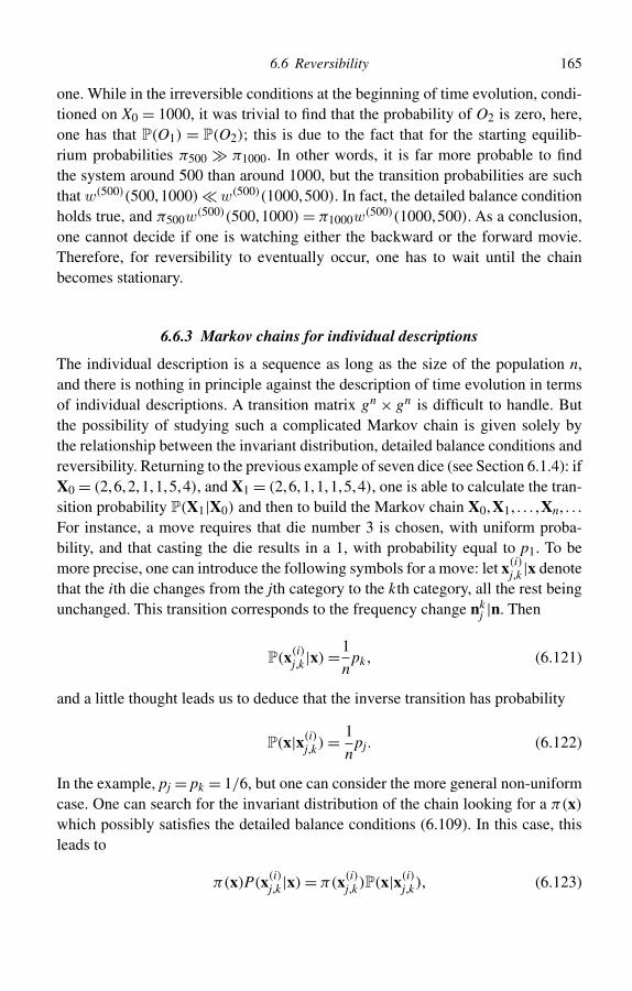
6.6 Reversibility 165
one. While in the irreversible conditions at the beginning of time evolution, condi-tioned on X0 = 1000, it was trivial to find that the probability of O2 is zero, here,one has that P(O1) = P(O2); this is due to the fact that for the starting equilib-rium probabilities π500 � π1000. In other words, it is far more probable to findthe system around 500 than around 1000, but the transition probabilities are suchthat w(500)(500,1000) � w(500)(1000,500). In fact, the detailed balance conditionholds true, and π500w
(500)(500,1000) = π1000w(500)(1000,500). As a conclusion,
one cannot decide if one is watching either the backward or the forward movie.Therefore, for reversibility to eventually occur, one has to wait until the chainbecomes stationary.
6.6.3 Markov chains for individual descriptions
The individual description is a sequence as long as the size of the population n,and there is nothing in principle against the description of time evolution in termsof individual descriptions. A transition matrix gn × gn is difficult to handle. Butthe possibility of studying such a complicated Markov chain is given solely bythe relationship between the invariant distribution, detailed balance conditions andreversibility. Returning to the previous example of seven dice (see Section 6.1.4): ifX0 = (2,6,2,1,1,5,4), and X1 = (2,6,1,1,1,5,4), one is able to calculate the tran-sition probability P(X1|X0) and then to build the Markov chain X0,X1, . . . ,Xn, . . .For instance, a move requires that die number 3 is chosen, with uniform proba-bility, and that casting the die results in a 1, with probability equal to p1. To bemore precise, one can introduce the following symbols for a move: let x(i)
j,k |x denotethat the ith die changes from the jth category to the kth category, all the rest beingunchanged. This transition corresponds to the frequency change nk
j |n. Then
P(x(i)j,k |x) =1
npk , (6.121)
and a little thought leads us to deduce that the inverse transition has probability
P(x|x(i)j,k) = 1
npj. (6.122)
In the example, pj = pk = 1/6, but one can consider the more general non-uniformcase. One can search for the invariant distribution of the chain looking for a π(x)
which possibly satisfies the detailed balance conditions (6.109). In this case, thisleads to
π(x)P(x(i)j,k |x) = π(x(i)
j,k)P(x|x(i)j,k), (6.123)
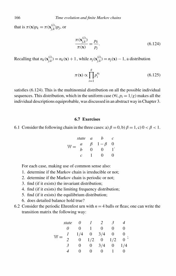
166 Time evolution and finite Markov chains
that is π(x)pk = π(x(i)j,k)pj, or
π(x(i)j,k)
π(x)= pk
pj. (6.124)
Recalling that nk(x(i)j,k) = nk(x)+ 1, while nj(x
(i)j,k) = nj(x)− 1, a distribution
π(x) ∝g∏
i=1
pnii (6.125)
satisfies (6.124). This is the multinomial distribution on all the possible individualsequences. This distribution, which in the uniform case (∀i, pi = 1/g) makes all theindividual descriptions equiprobable, was discussed in an abstract way in Chapter 3.
6.7 Exercises
6.1 Consider the following chain in the three cases: a) β = 0, b) β = 1, c) 0 < β < 1.
W =state a b c
a β 1 −β 0b 0 0 1c 1 0 0
.
For each case, making use of common sense also:1. determine if the Markov chain is irreducible or not;2. determine if the Markov chain is periodic or not;3. find (if it exists) the invariant distribution;4. find (if it exists) the limiting frequency distribution;5. find (if it exists) the equilibrium distribution;6. does detailed balance hold true?
6.2 Consider the periodic Ehrenfest urn with n = 4 balls or fleas; one can write thetransition matrix the following way:
W =
state 0 1 2 3 40 0 1 0 0 01 1/4 0 3/4 0 02 0 1/2 0 1/2 03 0 0 3/4 0 1/44 0 0 0 1 0
;
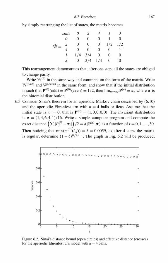
6.7 Exercises 167
by simply rearranging the list of states, the matrix becomes
W =
state 0 2 4 1 30 0 0 0 1 02 0 0 0 1/2 1/24 0 0 0 0 11 1/4 3/4 0 0 03 0 3/4 1/4 0 0
.
This rearrangement demonstrates that, after one step, all the states are obligedto change parity.
Write W(4) in the same way and comment on the form of the matrix. WriteW(odd) and W(even) in the same form, and show that if the initial distributionis such that P(0)(odd) = P(0)(even) = 1/2, then limn→∞ P(n) = π , where π isthe binomial distribution.
6.3 Consider Sinai’s theorem for an aperiodic Markov chain described by (6.10)and the aperiodic Ehrenfest urn with n = 4 balls or fleas. Assume that theinitial state is x0 = 0, that is P(0) = (1,0,0,0,0). The invariant distributionis π = (1,4,6,4,1)/16. Write a simple computer program and compute the
exact distance(∑ |P(t)
i −πi|)/2 = d(P(t),π) as a function of t = 0,1, . . . ,30.
Then noticing that min(w(4)(i, j)) = δ = 0.0059, as after 4 steps the matrixis regular, determine (1 − δ)(t/4)−1. The graph in Fig. 6.2 will be produced,
0 5 10 15 20 25 300
0.2
0.4
0.6
0.8
1
t
dist
ance
Figure 6.2. Sinai’s distance bound (open circles) and effective distance (crosses)for the aperiodic Ehrenfest urn model with n = 4 balls.
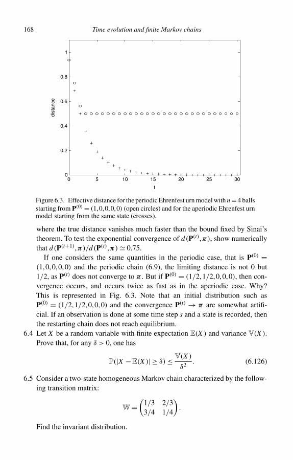
168 Time evolution and finite Markov chains
0 5 10 15 20 25 300
0.2
0.4
0.6
0.8
1
t
dist
ance
Figure 6.3. Effective distance for the periodic Ehrenfest urn model with n = 4 ballsstarting from P(0) = (1,0,0,0,0) (open circles) and for the aperiodic Ehrenfest urnmodel starting from the same state (crosses).
where the true distance vanishes much faster than the bound fixed by Sinai’stheorem. To test the exponential convergence of d(P(t),π), show numericallythat d(P(t+1),π)/d(P(t),π) 0.75.
If one considers the same quantities in the periodic case, that is P(0) =(1,0,0,0,0) and the periodic chain (6.9), the limiting distance is not 0 but1/2, as P(t) does not converge to π . But if P(0) = (1/2,1/2,0,0,0), then con-vergence occurs, and occurs twice as fast as in the aperiodic case. Why?This is represented in Fig. 6.3. Note that an initial distribution such asP(0) = (1/2,1/2,0,0,0) and the convergence P(t) → π are somewhat artifi-cial. If an observation is done at some time step s and a state is recorded, thenthe restarting chain does not reach equilibrium.
6.4 Let X be a random variable with finite expectation E(X ) and variance V(X ).Prove that, for any δ > 0, one has
P(|X −E(X )| ≥ δ) ≤ V(X )
δ2. (6.126)
6.5 Consider a two-state homogeneous Markov chain characterized by the follow-ing transition matrix:
W =(
1/3 2/33/4 1/4
).
Find the invariant distribution.
6.8 Summary 169
6.6 Evaluate W(t) for the transition probability matrix of Exercise 6.5 and fort = 2,5,10.
6.7 Consider a two-state homogeneous Markov chain characterized by the follow-ing transition matrix:
W =(
0 11 0
).
What happens to the powers Wt?
6.8 Summary
In this chapter, the following basic properties for irreducible Markov chains wereproved:
1. irreducibility leads to the existence of a (unique) invariant distribution π , whosemeaning is the limiting relative frequency of visiting times for any state (6.99);the ergodic theorem (6.103) is a consequence of this result;
2. aperiodicity further implies that the invariant distribution π is the equilib-rium distribution, that is lims→∞ P(Xs = j|X0 = x0) = πj, and the speed ofconvergence is geometric (exponential);
3. the main task in studying an irreducible Markov chain is to find the invariantdistribution π . One way is solving the eigenvalue problem discussed in Section6.5.1. However, given that the solution of the linear system (6.61) is practicallyimpossible in several applications to large physical and economic systems, thesearch for an invariant distribution must follow some other route;
4. the invariant distributionπ can be evaluated by means of a Monte Carlo computersimulation. As long as one sees that (hopefully) the histogram of relative visitingfrequencies stabilizes, one can apply Equation (6.99); this procedure is affectedby all the difficulties related to a frequency evaluation of probability. Also theMonte Carlo method soon becomes impractical for large systems;
5. given that a homogeneous irreducible Markov chain is reversible if and only if itis stationary and the stationary distribution satisfies the detailed balance condi-tions, imposing the detailed balance condition may help in finding the invariantdistribution. If the chain is irreducible, this is the unique invariant measure;moreover, if the chain is aperiodic, it is also the equilibrium distribution.
Further reading
The Ehrenfest urn model was introduced by Paul and Tatiana Ehrenfest in order tojustify Boltzmann’s ideas on statistical equilibrium.
170 Time evolution and finite Markov chains
P. Ehrenfest and T. Ehrenfest, Begriffliche Grundlagen der statistischen Auffassung inder Mechanik, in F. Klein and C. Müller (eds), Encyclopädie der Mathematischen Wis-senschaften mit Einschluß ihrer Anwendungen 4, 3–90, Teubner, Leipzig (1911). Englishtranslation in P. Ehrenfest and T. Ehrenfest, The Conceptual Foundations of the StatisticalApproach in Mechanics, Dover, New York (1990).
Marc Kac discusses this model in his book on the applications of probability theoryin physics:
M. Kac, Probability and Related Topics in Physical Science, Interscience, London (1959).
and it is now a standard subject in books on the application of probability theoryand stochastic processes to statistical physics.
H. Wio, An Introduction to Stochastic Processes and Nonequilibrium Statistical Physics,World Scientific, Singapore (1994).
Markov chains are named after Russian mathematician Andrey AndreyevichMarkov, who extended the weak law of large numbers and the central limit theorem(informally discussed below in Section 10.8) to the class of dependent random-variable sequences now carrying his name.
A.A. Markov, Rasprostranenie predel’nyh teorem ischisleniya veroyatnostej na summuvelichin svyazannyh v cep’, Zapiski Akademii Nauk po Fiziko-matematicheskomu otde-leniyu, VIII seriya, tom 25(3) (1908). English translation: A.A. Markov, Extension of theLimit Theorems of Probability Theory to a Sum of Variables Connected in a Chain, in R.A.Howard (ed.), Dynamic Probabilistic Systems, volume 1: Markov Chains, Wiley, New York(1971).
According to Basharin et al.,
G.P. Basharin, A.N. Langville and V.A. Naumov, The Life and Work of A. A. Markov, inA.N. Langville and W.J. Stewart (eds.), Proceedings of the 2003 conference on TheNumerical Solution of Markov Chains, Linear Algebra and its Applications, 386, 3–26(2004).
it was Bernstein
S. N. Bernstein, Sur l’extension du thèoréme du calcul de probabilités aux sommes dequantités dépendantes, Mathematische Annalen, 97, 1–59 (1926).
who used the name ‘Markov chains’ for the first time, to denote the processesdescribed in this chapter.
The reader can find an alternative and complete account on the theory of finiteMarkov chains in the classic book by Kemeny and Snell
J.G. Kemeny and J.L. Snell, Finite Markov Chains, Van Nostrand, Princeton, NJ (1960).
Hoel, Port and Stone present an exhaustive discussion on discrete Markov chainsin the first two chapters of their book on stochastic processes

References 171
P.G. Hoel, S.C. Port and C.J. Stone, Introduction to Stochastic Processes, Houghton Mifflin,Boston, MA (1972).
Our discussion of reversibility was inspired by
P. Suppes, Weak and Strong Reversibility of Causal Processes, in M.C. Gallavotti, P. Suppesand D. Costantini (eds.), Stochastic Causality, CSLI Publications, Stanford, CA (2001).
Finally, those interested in the extension of this theory to continuous state spacescan read the book by Meyn and Tweedie with profit
S.P. Meyn and R.L. Tweedie, Markov Chains and Stochastic Stability, Springer, Berlin(1993). S.P. Meyn and R.L. Tweedie, Markov Chains and Stochastic Stability, 2nd edition,Cambridge University Press, Cambridge, UK (2009).
References
[1] O. Penrose, Foundations of Statistical Mechanics, Pergamon Press, Oxford (1970).
7
The Ehrenfest–Brillouin model
Before studying this chapter, the reader is advised to (re-)read Section 6.1.4. In fact,the present chapter is devoted to a generalization of that example where random‘destructions’ are followed by ‘creations’ whose probability is no longer uniformover all the categories, but follows a rule due to L. Brillouin and directly related tothe Pólya distribution discussed in Chapter 5.
After reading this chapter, you should be able to:
• use random destructions (à la Ehrenfest) and Pólya distributed creations (à laBrillouin) to study the kinematics of a system of n elements moving within gcategories;
• define unary, binary, . . ., m-ary moves;• write the appropriate transition probabilities for these moves;• use detailed balance to find the invariant distribution for the Ehrenfest–Brillouin
Markov chain;• discuss some applications to economics, finance and physics illustrating the
generality of the Ehrenfest–Brillouin approach.
7.1 Merging Ehrenfest-like destructions and Brillouin-like creations
Statistical physics studies the macroscopic properties of physical systems at thehuman scale in terms of the properties of microscopic constituents. In 1996, Aokiexplicitly used such a point of view in economics, in order to describe macro vari-ables in terms of large collections of interacting microeconomic entities (agents,firms, and so on). These entities are supposed to change their state unceasingly,ruled by a Markov-chain probabilistic dynamics. All these situations are character-ized by a dynamical mechanism destroying an entity in a category and re-creatingan entity in another category. From an ontological point of view, in physics andeconomics, initial and final entities are usually the same, so that the destruction–creation mechanism can be interpreted just as a category change; this is the case
172
7.1 Merging Ehrenfest-like destructions and Brillouin-like creations 173
of the velocity change for a particle after a collision, or of the strategy variation ofan agent after a decision, and so on. On the contrary, in genetics, the destruction–creation mechanism can be interpreted as a death–birth process, where the twoentities are different, and even belong to different generations. In any case, in gen-eral, the elementary destruction–creation event depends on the present state of thewhole system. The state of the system, coinciding with the joint description of itsmicroscopic constituents, evolves as a consequence of these microscopic changes.If these features hold, the evolution is Markovian.
The Ehrenfest urn model can be seen as the starting point of this chapter. Oncethis model is considered as a ‘destruction–creation mechanism’, as in the aperi-odic version of Equation (6.5), it can be generalized in many ways, conservingthe original destruction mechanism, and using a more general creation term. If the‘creation probability’ is a function of the present occupation numbers, it can rep-resent correlations between agents, and the full transition probability still does notdepend on the time step leading to a homogeneous Markov chain. The ‘creationprobability’ introduced below is called ‘the Brillouin term’ for historical reasons.Both the Ehrenfests and Brillouin were physicists, and they essentially consideredparticles, cells and energy levels. However, nothing changes but the interpretationof quantities, when agents and strategies or firms and workers are considered.
As usual, consider a population made up of n entities (agents, particles, etc.) andg categories (cells, strategies, and so on). The state of the system is described bythe occupation number vector
n = (n1, . . . ,ni, . . . ,ng), (7.1)
with ni ≥ 0, and∑g
i=1 ni = n. Therefore, the state space is the set of g-ples summingup to n; this is denoted by
Sng = {n, ni ≥ 0,
∑ni = n}. (7.2)
The dynamical discrete-time evolution is given by the sequence of random variables
Y0 = n (0) ,Y1 = n (1) , . . . ,Yt = n (t) , . . . , (7.3)
where n (t) belongs to Sng . It is assumed that Equation (7.3) describes the realization
of a homogeneous Markov chain, whose one-step transition probability is a matrixwhose entries are given by
w(n,n′)= P(Yt+1 = n′|Yt = n), (7.4)
with n′,n ∈ Sng , not depending on time explicitly. How many entries has this
stochastic matrix?
174 The Ehrenfest–Brillouin model
7.2 Unary moves
The most elementary event considered here is: ‘an entity changes its state fromcategory i to category k’. Therefore, the state of the system changes from Yt = nto Yt+1 = nk
i , where n = (n1, . . . ,ni, . . . ,nk , . . . ,ng) denotes the initial state andnk
i = (n1, . . . ,ni −1, . . . ,nk +1, . . . ,ng) the final state, and the notation described inSection 6.1.1 is used. This transition can be split into two distinct parts. The first(the so-called ‘Ehrenfest’s term’) is the destruction of an entity belonging to the ithcategory, with probability
P(ni|n) = ni
n. (7.5)
The second part (the so-called ‘Brillouin’s term’) is the creation of a particle in thekth category given the vector ni = (n1,ni −1, . . . ,nk , . . . ,ng), whose probability is:
P(nki |ni) = αk + nk − δk,i
α + n − 1, (7.6)
with α =∑gi=1 αi, and α = (α1, . . . ,αg) is a vector of parameters; δk,i is the usual
Kronecker’s delta equal to 1 for k = i and zero otherwise. The meaning of αi isrelated to the probability of accommodation on the category i if it is empty. Twocases are interesting: all αi > 0, and all αi negative integers. In this second case,the size of the population is limited by the inequality n ≤ |α|, and categories withoccupation numbers ni = |αi| cannot accommodate further elements. The resultingtransition probability is:
P(nki |n) = P(ni|n)P(nk
i |ni) = ni
n
αk + nk − δk,i
α + n − 1. (7.7)
When all the αis are positive, if one starts from a given occupation vector n, byrepeated applications of (7.7), each possible vector of Sn
g can be reached withpositive probability. The cardinality of the state space is
#Sng =
(n + g − 1
n
). (7.8)
Moreover, all these states are persistent: in fact, given that αi > 0, an empty categorycan be occupied again. For negative integer αis, Equation (7.7) is understood toreturn zero if αk + nk − δk,i ≤ 0. The set of possible persistent states reduces to
Sng (|α|) =
{n :
g∑i=1
ni = n, ni ≤ |αi|}
, (7.9)
7.2 Unary moves 175
and starting from some initial state n ∈ Sng (|α|), all the states belonging to Sn
g (|α|)can be reached with positive probability.1 Therefore, the transition probability (7.7)describes an irreducible Markov chain. As a consequence of the discussion inChapter 6, there exists a unique invariant measure π(n) on the set of persistentstates. In addition, Equation (7.7) does not exclude the case n′ = nk
i = n, that is thecase k = j. Therefore, in all cases, the chain is aperiodic, due to the possibility for theselected element to immediately return into its original category. In other words, theinvariant measure π(n) is also the equilibrium distribution on the ergodic set and
limt→∞P(Yt = n|Y0 = n (0)) = π(n), (7.10)
irrespective of the initial state n0 = n(0).At a first glance, here, nothing is ‘irreversible’ in the transition mechanism. Then,
the search for the invariant distribution can be done by means of detailed balanceconditions. Indeed, using Equations (6.109) and (7.7) for i �= j, one finds that
π(nki )
π(n)= ni
nk + 1
αk + nk
αj + nj − 1, (7.11)
a relationship which is satisfied by the generalized g-dimensional Pólya distribution(see Chapter 5)
π(n) = Pólya(n;α) = n!α[n]
g∏i=1
α[ni]i
ni! , (7.12)
with∑g
i=1 ni = n and∑g
i=1 αi = α. If {αi > 0}, then creations are positively corre-lated with occupation numbers n. The equilibrium probability (7.12) can be relatedto a Pólya urn scheme with initial composition α and unitary prize. A simple sub-case of Equation (7.12) is the so-called Bose–Einstein distribution, which is thesymmetric g-dimensional Pólya distribution with αi = 1, and α = g. In this caseα
[ni]i becomes ni!, and
n!α[n] = n!
g[n] , (7.13)
so that one eventually finds
πBE(n) = Pólya(n;1) =(
n + g − 1
n
)−1
, (7.14)
1 For instance, if one starts from n =(n,0, . . . ,0),n ≤ |α|, and n > |α1| from Equation (7.7), it turns out that n1is forced to decrease until the value n1 = |α1| is reached, and n1 will never become greater than |α1| again.Therefore, all the states with n ≤ |α| and with some ni > |αi| are not persistent (they are called transient states).Hence, also in this unusual case after a finite number of steps the dynamics is restricted to the set Sn
g (|α|) ofEquation (7.9).
176 The Ehrenfest–Brillouin model
where α = 1 = (1, . . . ,1) is a vector containing g values equal to 1. In other words,if α = 1, all the occupation vectors have the same equilibrium probability, that isπBE does not depend on n. When {αi < 0} and αi are negative integers, creationsare negatively correlated with the occupation numbers n. The equilibrium proba-bility (7.12) becomes the g-dimensional hypergeometric distribution, that can bere-written as
π(n) = HD(n; |α|) =∏g
i=1
(|αi|ni
)(|α|
n
) , (7.15)
with∑g
i=1 ni = n, and ni ≤ |αi|. A remarkable example of Equation (7.15) is theso-called Fermi–Dirac distribution, which is obtained for αi = −1, and α = −g.Given that ni ∈ {0,1}, the numerator is 1, and one finds that
πFD(n) = Pólya(n;−1) =(
g
n
)−1
, (7.16)
which is uniform on all occupation vectors with ni ∈ {0,1}, as also πFD does notdepend on n. Note that both πBE and πFD are the only uniform distributions on theoccupation vectors in the two possible domains of α. They are at the basis of thestatistical description of quantum particles.
The correlation is large and positive for small α > 0, it is large and negative forsmall (integer) α < 0. The smallest possible value of α < 0 is α = −g, where nomore than one unit can occupy each category (this is known in physics as Pauli’sexclusion principle). Correlations vanish for |α| → ∞ from both sides, where thecreation probability becomes pk = αk/α independent of n. In this limit, Equation(7.12) becomes
π(n) = Pólya(n;±∞) = MD(n;p) = n!∏gi=1 ni!
g∏i=1
pnii , (7.17)
which is the multinomial distribution; if p1 = p2 = . . . = pn = 1/g, one gets thesymmetric multinomial distribution
πMB(n) = n!∏gi=1 ni!
g−n; (7.18)
in statistical physics, this is known as the Maxwell–Boltzmann distribution. The case|α| → ∞ coincides with an independent accommodation of the moving element;it was discussed in Sections 6.1.2 and 6.1.4. The equilibrium probability (7.18) is
7.3 From fleas to ants 177
such that all the individual descriptions X are equiprobable,2 and this distributionlies at the foundation of classical statistical mechanics.
It is interesting to observe that all the above distributions can be discussed ina unified way within the same probabilistic scheme, without introducing notionssuch as ‘(in-)distinguishable’particles or elements, which are sometimes used evenin probability (by Feller for instance) and in economics. The different behaviour ofthe microscopic entities is due to the vector parameter α leading to different kindsof inter-element correlation.
In statistical physics, the cases of Equations (7.14), (7.16) and (7.18) exhaustall the possibilities. In economics, the so-called ‘parastatistics’ are possible, whichseem forbidden in physics. This issue will be further discussed in Chapter 8.
7.3 From fleas to ants
The Ehrenfest–Brillouin model is more powerful than the Ehrenfest urn models dueto probabilistic creations depending on the state of the system. Ehrenfest’s fleas arerandomly selected, and they must change dog. The creation is then deterministic(it happens with probability 1). In the aperiodic version, the selected flea choosesthe new dog tossing a coin. Here, creation is probabilistic, but independent of thestate of the system. What is the meaning of a creation probability with the formof Equation (7.6)? Consider the case k �= i, just to avoid the term δk,i. Introducingpk = αk/α, the probability of occupying cell k given that the present occupationvector is Y(n−1) = ni, with
∑i y(n−1)
i = n − 1, can be re-written as
P(nki |ni) = αpk + nk
α + n − 1= α
α + n − 1pk + n − 1
α + n − 1
nk
n − 1. (7.19)
In selecting a category, the moving element uses two probability distributions,an ‘initial’ (or theoretical) distribution {pk}g
k=1 and an ‘empirical’ distribution{nk/(n−1)}g
k=1, given by the relative accommodation frequency of the n−1 otherelements. Equation (7.19) can be regarded as a weighted average (mixture) of thetwo distributions, where α is the weight of the initial distribution, and n − 1 isthe weight of the empirical one. The theoretical and empirical distributions are theextremes of a simplex, able to represent both independence (α � n) and strongcorrelation (α � n). This mixture can be seen as a randomization of two strategies,following Kirman’s ideas (see Further reading). One can interpret the moving ele-ments as economic agents and the categories as strategies followed by the agents.Assume that the choice is performed in two stages: first the choice of the distribution,followed by the choice of the category given the chosen distributions. Focusing on
2 This means that the distribution on the set of the gn possible individual descriptions is uniform.
178 The Ehrenfest–Brillouin model
a category/strategy, say the kth strategy, one can write for the creation term (7.19)
P(C = k) = P(C = k|Theor)P(Theor)+P(C = k|Emp)P(Emp), (7.20)
where C = k denotes a creation in the kth category given ni
P(C = k|Theor) = pk , (7.21)
and
P(C = k|Emp) = nk
n − 1, (7.22)
whereas
P(Theor) = α
α + n − 1, (7.23)
and
P(Emp) = n − 1
α + n − 1. (7.24)
If a moving agent chooses the theoretical distribution (behaving as a ‘fundamental-ist’), she is not influenced by her colleagues. In this case, one has a self-modificationof behaviour. If a moving agent chooses the empirical distribution (behaving as a‘chartist’), then he chooses a colleague at random and he selects her strategy. This isexactly the ant foraging behaviour model introduced by Kirman in the very specialcase of two symmetric sources of food. The ‘strange’ behaviour of the ants is suchthat one can find almost all of them at the same food source for a long time, andthe change from one source to the other is similar to an avalanche. On average,the two sources are exploited in the same way, and the equilibrium distributionis U-shaped. This behaviour is just the opposite of the Ehrenfest case, with fleashopping onto two dogs, where the equilibrium distribution is bell-shaped. The gen-eralization presented here admits g sources of food, and a general initial probabilitydistribution
(p1, . . . ,pk , . . . ,pg
)that may reflect objective differences (‘fundamen-
tals’) between the sources. The original Kirman’s model can be formulated as abirth–death Markov chain by means of the following general transition probabili-ties, which work in the case of fleas, as well. Focusing again on a single categoryand setting w(k,h) = P(Yt+1 = h|Yt = k), one has
w(k,k + 1) = n − k
n
(α/2)+ k
α + n − 1, (7.25)
w(k,k − 1) = k
n
(α/2)+ n − k
α + n − 1, (7.26)
7.3 From fleas to ants 179
and
w(k,k) = 1 −w(k,k + 1)−w(k,k − 1), (7.27)
with all the other transitions forbidden. The ‘normal’ behaviour of fleas is obtainedby letting α → ∞ (see Equation (6.10)), whereas the ‘strange’ ant behaviour isobtained setting α = 1. Following the discussion in the previous section, the equi-librium distribution for fleas is the binomial distribution of parameter p = 1/2; inother words, one has
πfleas(k) = Bin(k;n,1/2), (7.28)
whereas the equilibrium distribution for Kirman’s ants is
πants(k) = Pólya(k,n − k;1/2,1/2), (7.29)
a U-shaped distribution. In this case, in the continuous limit k � 1, n � 1, thefraction x = k/n is distributed according to the Beta distribution, whose probabil-ity density function Beta (x;1/2,1/2) is proportional to 1/
(√x(1 − x)
). Note that
E(Y ) = n/2 in both cases (they are both symmetric distributions), whereas thevariance depends on α and is given by
V(Y ) = n
4
(α + n
α + 1
), (7.30)
which is proportional to n2 for ants (and to n for fleas). Indeed, the ant model isnon-self-averaging (see Chapter 5).
Given that both ants and (aperiodic) fleas share the same probabilistic engine(Equations (7.25), (7.26) and (7.27)), their behaviour can be simulated with the sameprogram (code), where the weight of the initial distribution α can be continuouslychanged from large values α � 1 (see also Exercise 5.5 and Fig. A5.5) to Kirman’svalue α = 1 (see Exercise 7.2 below).
Another important difference between the cases α → ∞ (independent accom-modations) and α = 1 (strong herding behaviour) is given by the rate of approach toequilibrium. While fleas run very fast towards the equilibrium ‘fifty–fifty’situation,and after that oscillate around the expected value, ants stay for a long time at onefood source, and they suddenly rush to the other source, as an avalanche; moreover,they are seldom found in the expected ‘fifty–fifty’ situation. Later, it will be shownthat the number of steps needed for the expected value to reach its equilibriumvalue is roughly n(α + n − 1)/α, which gives exactly n for fleas, but n2 for ants.
In Kirman’s original formulation the weight of the theoretical distribution is δ andthe empirical weight is 1−δ, independent of the population size. In his framework,in order to get the beta distribution, it is necessary to assume that n → ∞, δ → 0 and
180 The Ehrenfest–Brillouin model
nδ → α. On the contrary, in the Equations (7.25), (7.26) and (7.27), the empiricalweight depends on the size of population from the beginning. It is quite reasonableto imagine that the weight of the ‘herding behaviour’ is just the size of the herd.This weight must be compared to α, the weight of ‘self-modification’.
7.4 More complicated moves
Unary moves are the smallest and simplest changes that can take place in a popula-tion.As briefly discussed above, the marginal Ehrenfest–Brillouin model belongs tothe family of birth–death Markov chains, admitting a continuous limit both in spaceand in time (see also Section 10.8 below). However, more complicated moves areneeded in many applications. For instance, in physics, interparticle collisions causea change of category (state) of two particles. A binary collision is represented bytwo particles in the initial categories (also called cells in this case) (i, j) and endingin the final categories (k, l). A binary transition can be represented by nkl
ij |n, where
n = (n1, . . . ,ni, . . . ,nj, . . . ,nk , . . . ,nl , . . . ,ng), (7.31)
and
nklij = (n1, . . . ,ni − 1, . . . ,nj − 1, . . . ,nk + 1, . . . ,nl + 1, . . . ,ng). (7.32)
A generalization of Equations (7.7) to binary moves is the following, for i, j,k, l alldifferent:
P(nklij |n) = P(nij|n)P(nkl
ij |nij) = 4ni
n
nj
n − 1
(αk + nk)(αl + nl)
(α + n − 2)(α + n − 1). (7.33)
Neglecting the coefficient 4, the first two terms give the probability of selecting aparticle in the ith cell, followed by the extraction of a particle in cell j in a hyperge-ometric process of parameter n, where n is the initial occupation vector. The thirdterm is an accommodation Pólya process with weights αk +nk for the kth cell whenthe total weight is α + n − 2, and the fourth is an accommodation Pólya processwith weights αl + nl and total weight given by α + n − 1. This mechanism is justthe same as for unary moves, considering that each destruction or creation step isconditioned to the current state of the population and that the population diminishesduring destructions, and increases during creations. The factor 4 is due to the fourpaths connecting n to nkl
ij . In fact, denote by D1 = i, D2 = j, C1 = k, C2 = l thesequence of the two extractions followed by the two accommodations. There are twodestruction sequences connecting n to nij, that is D1 = i,D2 = j and D1 = j,D2 = i,and there are two creation sequences from nij to nkl
ij , that is C1 = k, C2 = l andC1 = l, C2 = k. Due to the exchangeability of destructions {Dr} and creations {Cr},
7.5 Pólya distribution structures 181
the four paths D1, D2, C1, C2 are equiprobable. The coefficient is not 4 if some indexis repeated, but these subtleties can be omitted. The simplest route to the invariantdistribution is using the detailed balance conditions, and showing that the invariantdistribution of (7.33) is still the Pólya distribution (7.12). However, a more refinedapproach is possible, based on a deep property of the Pólya distribution.
7.5 Pólya distribution structures
Consider ten ‘fair’ coins on a table, which were ‘honestly’ tossed, but they arecovered and the result of the tosses is not known. Then a coin is removed fromthe table; whether it was ‘heads’ or ‘tails’ is unknown, all coins being on a par forbeing removed. What can be said about the probability distribution of the remainingcoins? In order to formally discuss this problem, note that one has a population often elements which can belong to two categories; focusing on the occupation vectorn = (nH,nT), with n = 10 = nH + nT, and defining k = nH, one has that
P10(k) =(
10
k
)2−10, k = 0,1, . . . ,10. (7.34)
Now an element is selected at random, and the probability P9(k) is desired, fork = 0,1, . . . ,9. Consider the case in which on the table there are 2 heads (and 7tails), whose probability is P9(2). This event is consistent with two hypotheses:either there were 3 heads on the table (an event with probability P10(3)) and a headwas removed (with conditional probability 3/10), or there were 2 heads on thetable (an event with probability P10(2)) and a tail was removed (with conditionalprobability 8/10). Then, one finds that
P9(2) = (3/10)P10(3)+ (8/19)P10(2); (7.35)
this result can be generalized to any number n of coins, leading to the followingequation
Pn−1(k) = Pn(k + 1)k + 1
n+Pn(k)
n − k
n. (7.36)
One can directly verify that if Pn(k) = Bin(k;n,p), then one has Pn−1(k) =Bin(k;n−1,p). In other words, hypergeometric sampling does conserve the struc-ture of the probability distribution. Returning to the problem discussed above, itssolution is
P9(2) =(
9
2
)2−9. (7.37)
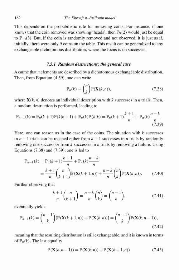
182 The Ehrenfest–Brillouin model
This depends on the probabilistic rule for removing coins. For instance, if oneknows that the coin removed was showing ‘heads’, then P9(2) would just be equalto P10(3). But, if the coin is randomly removed and not observed, it is just as if,initially, there were only 9 coins on the table. This result can be generalized to anyexchangeable dichotomous distribution, where the focus is on successes.
7.5.1 Random destructions: the general case
Assume that n elements are described by a dichotomous exchangeable distribution.Then, from Equation (4.59), one can write
Pn(k) =(
n
k
)P(X(k,n)), (7.38)
where X(k,n) denotes an individual description with k successes in n trials. Then,a random destruction is performed, leading to
Pn−1(k) = Pn(k + 1)P(k|k + 1)+Pn(k)P(k|k) = Pn(k + 1)k + 1
n+Pn(k)
n − k
n.
(7.39)
Here, one can reason as in the case of the coins. The situation with k successesin n − 1 trials can be reached either from k + 1 successes in n trials by randomlyremoving one success or from k successes in n trials by removing a failure. UsingEquations (7.38) and (7.39), one is led to
Pn−1(k) = Pn(k + 1)k + 1
n+Pn(k)
n − k
n
= k + 1
n
(n
k + 1
)P(X(k + 1,n))+ n − k
n
(n
k
)P(X(k,n)). (7.40)
Further observing that
k + 1
n
(n
k + 1
)= n − k
n
(n
k
)=(
n − 1
k
), (7.41)
eventually yields
Pn−1(k) =(
n − 1
k
)[P(X(k + 1,n))+P(X(k,n))] =
(n − 1
k
)P(X(k,n − 1)),
(7.42)
meaning that the resulting distribution is still exchangeable, and it is known in termsof Pn(k). The last equality
P(X(k,n − 1)) = P(X(k,n))+P(X(k + 1,n)) (7.43)
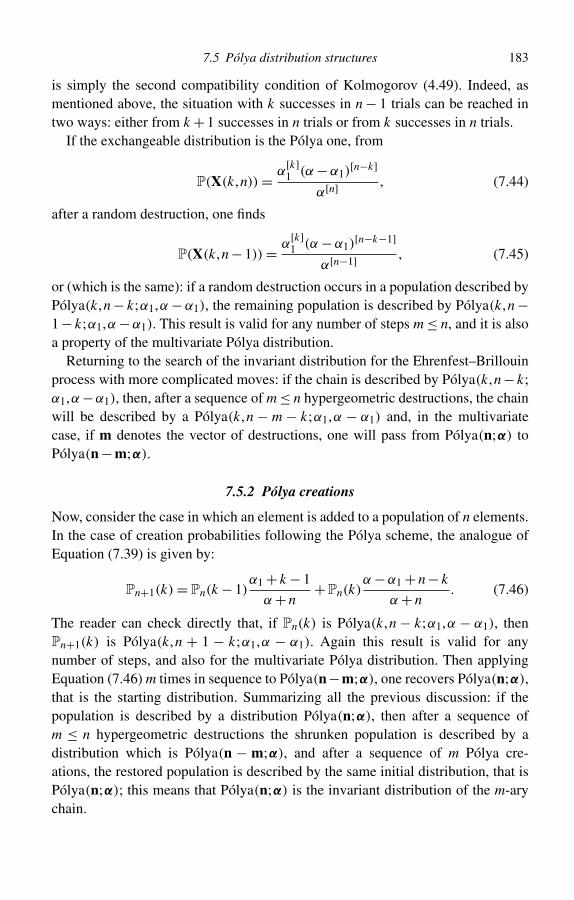
7.5 Pólya distribution structures 183
is simply the second compatibility condition of Kolmogorov (4.49). Indeed, asmentioned above, the situation with k successes in n − 1 trials can be reached intwo ways: either from k + 1 successes in n trials or from k successes in n trials.
If the exchangeable distribution is the Pólya one, from
P(X(k,n)) = α[k]1 (α −α1)
[n−k]
α[n] , (7.44)
after a random destruction, one finds
P(X(k,n − 1)) = α[k]1 (α −α1)
[n−k−1]
α[n−1] , (7.45)
or (which is the same): if a random destruction occurs in a population described byPólya(k,n − k;α1,α −α1), the remaining population is described by Pólya(k,n −1 − k;α1,α −α1). This result is valid for any number of steps m ≤ n, and it is alsoa property of the multivariate Pólya distribution.
Returning to the search of the invariant distribution for the Ehrenfest–Brillouinprocess with more complicated moves: if the chain is described by Pólya(k,n − k;α1,α −α1), then, after a sequence of m ≤ n hypergeometric destructions, the chainwill be described by a Pólya(k,n − m − k;α1,α − α1) and, in the multivariatecase, if m denotes the vector of destructions, one will pass from Pólya(n;α) toPólya(n − m;α).
7.5.2 Pólya creations
Now, consider the case in which an element is added to a population of n elements.In the case of creation probabilities following the Pólya scheme, the analogue ofEquation (7.39) is given by:
Pn+1(k) = Pn(k − 1)α1 + k − 1
α + n+Pn(k)
α −α1 + n − k
α + n. (7.46)
The reader can check directly that, if Pn(k) is Pólya(k,n − k;α1,α − α1), thenPn+1(k) is Pólya(k,n + 1 − k;α1,α − α1). Again this result is valid for anynumber of steps, and also for the multivariate Pólya distribution. Then applyingEquation (7.46) m times in sequence to Pólya(n−m;α), one recovers Pólya(n;α),that is the starting distribution. Summarizing all the previous discussion: if thepopulation is described by a distribution Pólya(n;α), then after a sequence ofm ≤ n hypergeometric destructions the shrunken population is described by adistribution which is Pólya(n − m;α), and after a sequence of m Pólya cre-ations, the restored population is described by the same initial distribution, that isPólya(n;α); this means that Pólya(n;α) is the invariant distribution of the m-arychain.
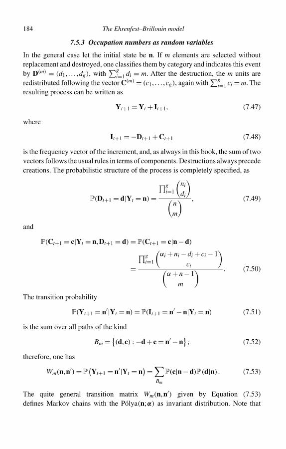
184 The Ehrenfest–Brillouin model
7.5.3 Occupation numbers as random variables
In the general case let the initial state be n. If m elements are selected withoutreplacement and destroyed, one classifies them by category and indicates this eventby D(m) = (d1, . . . ,dg), with
∑gi=1 di = m. After the destruction, the m units are
redistributed following the vector C(m) = (c1, . . . ,cg), again with∑g
i=1 ci = m. Theresulting process can be written as
Yt+1 = Yt + It+1, (7.47)
where
It+1 = −Dt+1 + Ct+1 (7.48)
is the frequency vector of the increment, and, as always in this book, the sum of twovectors follows the usual rules in terms of components. Destructions always precedecreations. The probabilistic structure of the process is completely specified, as
P(Dt+1 = d|Yt = n) =∏g
i=1
(ni
di
)(
n
m
) , (7.49)
and
P(Ct+1 = c|Yt = n,Dt+1 = d) = P(Ct+1 = c|n − d)
=∏g
i=1
(αi + ni − di + ci − 1
ci
)(
α + n − 1
m
) . (7.50)
The transition probability
P(Yt+1 = n′|Yt = n) = P(It+1 = n′ − n|Yt = n) (7.51)
is the sum over all paths of the kind
Bm = {(d,c) : −d + c = n′ − n}
; (7.52)
therefore, one has
Wm(n,n′) = P(Yt+1 = n′|Yt = n
)=∑Bm
P(c|n − d)P(d|n) . (7.53)
The quite general transition matrix Wm(n,n′) given by Equation (7.53)defines Markov chains with the Pólya(n;α) as invariant distribution. Note that
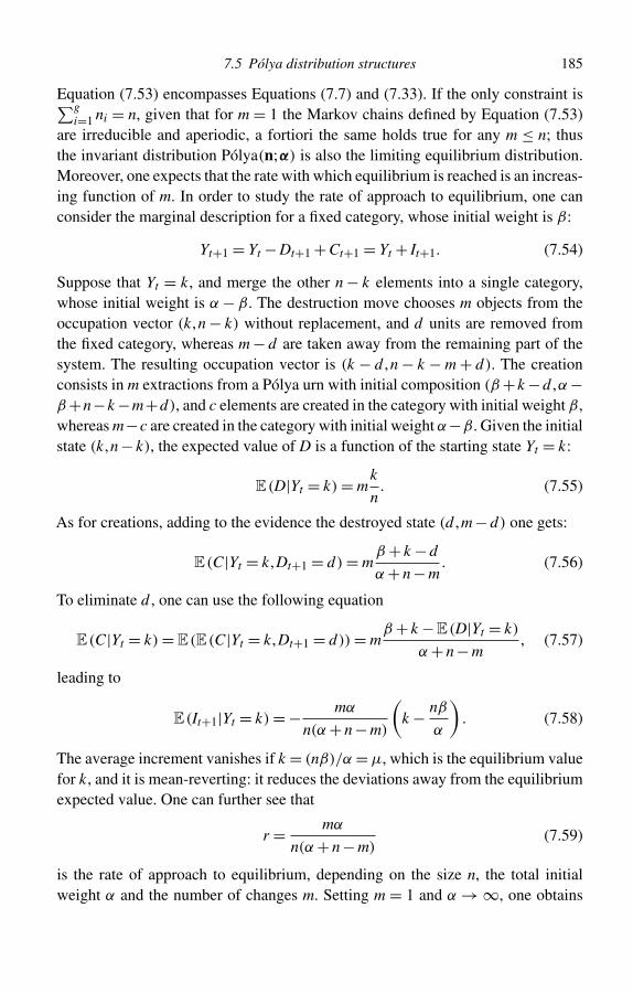
7.5 Pólya distribution structures 185
Equation (7.53) encompasses Equations (7.7) and (7.33). If the only constraint is∑gi=1 ni = n, given that for m = 1 the Markov chains defined by Equation (7.53)
are irreducible and aperiodic, a fortiori the same holds true for any m ≤ n; thusthe invariant distribution Pólya(n;α) is also the limiting equilibrium distribution.Moreover, one expects that the rate with which equilibrium is reached is an increas-ing function of m. In order to study the rate of approach to equilibrium, one canconsider the marginal description for a fixed category, whose initial weight is β:
Yt+1 = Yt − Dt+1 + Ct+1 = Yt + It+1. (7.54)
Suppose that Yt = k, and merge the other n − k elements into a single category,whose initial weight is α − β. The destruction move chooses m objects from theoccupation vector (k,n − k) without replacement, and d units are removed fromthe fixed category, whereas m − d are taken away from the remaining part of thesystem. The resulting occupation vector is (k − d ,n − k − m + d). The creationconsists in m extractions from a Pólya urn with initial composition (β + k −d ,α −β +n−k −m+d), and c elements are created in the category with initial weight β,whereas m−c are created in the category with initial weight α−β. Given the initialstate (k,n − k), the expected value of D is a function of the starting state Yt = k:
E(D|Yt = k) = mk
n. (7.55)
As for creations, adding to the evidence the destroyed state (d ,m − d) one gets:
E(C|Yt = k,Dt+1 = d) = mβ + k − d
α + n − m. (7.56)
To eliminate d , one can use the following equation
E(C|Yt = k) = E(E(C|Yt = k,Dt+1 = d)) = mβ + k − E(D|Yt = k)
α + n − m, (7.57)
leading to
E(It+1|Yt = k) = − mα
n(α + n − m)
(k − nβ
α
). (7.58)
The average increment vanishes if k = (nβ)/α = µ, which is the equilibrium valuefor k, and it is mean-reverting: it reduces the deviations away from the equilibriumexpected value. One can further see that
r = mα
n(α + n − m)(7.59)
is the rate of approach to equilibrium, depending on the size n, the total initialweight α and the number of changes m. Setting m = 1 and α → ∞, one obtains
186 The Ehrenfest–Brillouin model
r = 1/n, the value for the unary Ehrenfest aperiodic model. The rate is a linearfunction of m if m � n, and grows to 1 for m = n. Note that for m = n, and r = 1,the destruction completely empties the system, so that, all at once, the subsequentcreation probability is already the equilibrium one. In this limiting case Yt+1 does notdepend on Yt , and one expects a vanishing correlation C(Yt ,Yt+1) = 0. Therefore,one can derive the equation
E(It+1|Yt = k) = −r (k −µ) , (7.60)
or equivalently, adding k − µ to both sides and taking out of the expected valuewhat is known
E(Yt+1|Yt = k)−µ = (1 − r)(k −µ) . (7.61)
The expected increment acts as a restoring force, making the new expected positioncloser to the equilibrium value. Iterating Equation (7.61), one finds
E(Yt+s|Yt = k)−µ = (1 − r)s (k −µ) . (7.62)
Introducing the ‘centred variable’ Ut = Yt −µ, whose equilibrium value is µU = 0,and letting q = 1 − r, the evolution Equation (7.62) reduces to
E(Ut+s|Ut = u) = qsu, (7.63)
and taking the expectation on both sides
E(Ut+s) = qsE(Ut). (7.64)
All these equations show that the regression of Yt+1 on Yt , that is, by definition, theexpected value of Yt+1 conditioned on Yt , is linear, proportional to Yt .
This is a simple example (restricted to the first moment) of the general geometricalapproach to equilibrium for all Markov chains (see Chapter 6). Note that It+1 =Yt+1 − Yt = Ut+1 − Ut ; therefore, passing to the second centred moments, whichare the same for Y and U , one gets
C(Yt+1,Yt) = C(Ut+1,Ut) = E(Ut+1Ut)−E(Ut+1)E(Ut). (7.65)
Now, one has that
E(Ut+1)E(Ut) = qE2(Ut), (7.66)
as E(Ut+1) = qE(Ut). Moreover, one can write
E(Ut+1Ut) = E(E(Ut+1Ut|Ut = u)) = qE(U 2t ), (7.67)
7.5 Pólya distribution structures 187
as a consequence of Equation (7.63). Finally, replacing Equations (7.66) and (7.67)into Equation (7.65), one finds that
C(Yt+1,Yt) = C(Ut+1,Ut) = q[E(U 2t )−E2(Ut)] = qV(Ut). (7.68)
This is another way of showing the linear regression, as Equation (7.61) can bere-written in the following way:
E(Ut+1|Ut = u) = qu, (7.69)
that is the regression of Ut+1 on Ut is linear, and the angular coefficient b of theregression line of Ut+1 on Ut is a constant
b = C(Ut+1,Ut)
V(Ut)= q = 1 − r, (7.70)
and the equation of the regression line is
E(Ut+1|Ut = u)−E(Ut+1) = q(u −E(Ut)), (7.71)
obtained from E(Ut+1) = qE(Ut), subtracted from both sides of Equation (7.69).Although both C(Ut+1,Ut) and V(Ut) are difficult to calculate in the general case,their ratio is known also far from equilibrium.
When the chain reaches equilibrium, it becomes stationary and both E(Ut+1)
and E(Ut) vanish, and E(U 2t ) converges to V(Xt) → σ 2, where
σ 2 = nβ
α
(1 − β
α
)(α + n
α + 1
), (7.72)
and
C(Yt+1,Yt) = C(Ut+1,Ut) = (1 − r)σ 2 = qσ 2, (7.73)
and, iterating Equation (7.73), one finds
C(Yt+s,Yt) = (1 − r)sσ 2. (7.74)
Then the Bravais–Pearson autocorrelation function of the process once it attainsstationarity is
ρ (Yt+s,Yt) = ρ(s) = (1 − r)s. (7.75)
The variance of increments is
V(It+1) = E(U 2t+1)+E(U 2
t )− 2C(Ut+1,Ut) = 2σ 2 − 2(1 − r)σ 2 = 2rσ 2.(7.76)
188 The Ehrenfest–Brillouin model
Suppose two categories are considered, and call K and L the respective occu-pation variables; the two categories evolve in time against the rest of the system,which simulates a thermostat. In the thermodynamic limit, when the rest of the sys-tem is very large, K and L become uncorrelated and even independent (see Section7.6); this means that for any s:
C(Kt+s,Kt) = (1 − r)sσ 2K ,
C(Lt+s,Lt) = (1 − r)sσ 2L ,
C(Lt+s,Kt) = 0 for any s. (7.77)
Then considering the random variable V = K − L, one has
V(Vt) = σ 2K +σ 2
L = σ 2V , (7.78)
and
C(Vt+s,Vt) = C(Kt+s,Kt)+C(Lt+s,Lt) = (1 − r)s(σ 2K +σ 2
L ) = (1 − r)sσ 2V .
(7.79)
These equations lead to the following Bravais–Pearson autocorrelation function
ρ (Vt+s,Vt) = (1 − r)s. (7.80)
Summarizing all the previous results, Equation (7.47), with probability condi-tions (7.49), (7.50) and (7.53), defines a random walk on the set of states n ∈Sg
n ,whose degree of time correlation is triggered by m ≤ n, ceteris paribus. If mincreases, the Bravais–Pearson autocorrelation function ρ (Yt+1,Yt) diminishes,and, in the case m = n, it vanishes because the variables Yt become independent.This feature is important in applications, as this model is very flexible and canrepresent empirical time series with very different time-correlation behaviour (seeExercise 7.1, as well).
7.6 An application to stock price dynamics
The previous model can be applied to price increments (or returns) in a stock market.Consider a stock market with n agents, labelled from 1 to n, trading a single riskyasset, whose log-price at time step t is denoted by the random variable X (t). Duringeach time period, an agent may choose either to buy, or to sell or not to trade. Thequantity of shares requested by agent i is represented by the random variable �i,which can assume three values +1 (bullish behaviour: agent i wants to buy hopingthat the price will increase), 0 (neutral behaviour, agent i does not want either tosell or to buy) and −1 (bearish behaviour: agent i wants to sell fearing that the
7.6 An application to stock price dynamics 189
price will decrease). The aggregate excess demand for the risky asset at time t isthen given by
D (t) =n∑
i=1
�i (t) . (7.81)
Assume that the price log-return is proportional to D(t):
X (t) = X (t + 1)− X (t) = 1
ηD(t) = 1
η
n∑i=1
�i(t), (7.82)
where η is the excess demand needed to move the return of one unit. In the followingη = 1 for the sake of simplicity. In order to evaluate the distribution of returns, oneneeds the joint distribution of {�i (t)}i=1,...,n. There are three strategies (bullish,bearish, neutral) and n agents. The state of the system is denoted by the occupationvector n = (n+,n−,n0). This allows us to treat the number of active agents n+ +n−as a random variable. The excess demand is given by D(t) = n+(t) − n−(t). Theparameters α+ = a, α− = b and α0 = c = θ −a −b, with θ = a +b+ c, associatedto the three strategies, determine the transition probabilities of a Markov chain. Inthis framework, the financial interpretation should be clear. At each time step, afixed number m of agents has the possibility of changing strategy. The fraction m/nis the percentage of agents that, at each step, are involved in strategy changes. Forpositive initial weights the moving agent tends to join the majority (this is knownas herding behaviour); for negative weights, the selected agent tends to behave atodds with the current majority’s behaviour (this is known as contrarian behaviour);for very large weights agents are not influenced by their environment.
If the probabilistic dynamics follows Equation (7.47), with the usual prob-ability conditions (7.49), (7.50) and (7.53), the equilibrium distribution is thethree-dimensional Pólya distribution, that is (i ∈ {+,−,0}),
π (n) = π (n+,n−,n0) = n!θ [n]
∏i
α[ni]i
ni! , (7.83)
with the constraint n+ + n− + n0 = n. As mentioned before, the effective demand∑ni=1 �i (t) = n+(t)−n−(t) is a function of n. Now the ‘thermodynamic limit’ can
be introduced. In the limit α0 = c → ∞, n → ∞, with χ = n/θ kept constant, thePólya distribution factorizes, leading to
π (n+,n−,n0 = n − n+ − n−) → P(n+)P(n−) , (7.84)
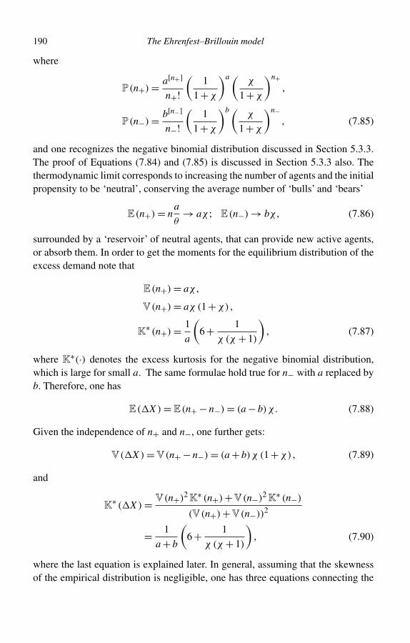
190 The Ehrenfest–Brillouin model
where
P(n+) = a[n+]
n+!(
1
1 +χ
)a(χ
1 +χ
)n+,
P(n−) = b[n−]
n−!(
1
1 +χ
)b(χ
1 +χ
)n−, (7.85)
and one recognizes the negative binomial distribution discussed in Section 5.3.3.The proof of Equations (7.84) and (7.85) is discussed in Section 5.3.3 also. Thethermodynamic limit corresponds to increasing the number of agents and the initialpropensity to be ‘neutral’, conserving the average number of ‘bulls’ and ‘bears’
E(n+) = na
θ→ aχ ; E(n−) → bχ , (7.86)
surrounded by a ‘reservoir’ of neutral agents, that can provide new active agents,or absorb them. In order to get the moments for the equilibrium distribution of theexcess demand note that
E(n+) = aχ ,
V(n+) = aχ (1 +χ) ,
K∗ (n+) = 1
a
(6 + 1
χ (χ + 1)
), (7.87)
where K∗(·) denotes the excess kurtosis for the negative binomial distribution,which is large for small a. The same formulae hold true for n− with a replaced byb. Therefore, one has
E( X ) = E(n+ − n−) = (a − b)χ . (7.88)
Given the independence of n+ and n−, one further gets:
V( X ) = V(n+ − n−) = (a + b)χ (1 +χ) , (7.89)
and
K∗ ( X ) = V(n+)2 K∗ (n+)+V(n−)2 K∗ (n−)
(V(n+)+V(n−))2
= 1
a + b
(6 + 1
χ (χ + 1)
), (7.90)
where the last equation is explained later. In general, assuming that the skewnessof the empirical distribution is negligible, one has three equations connecting the
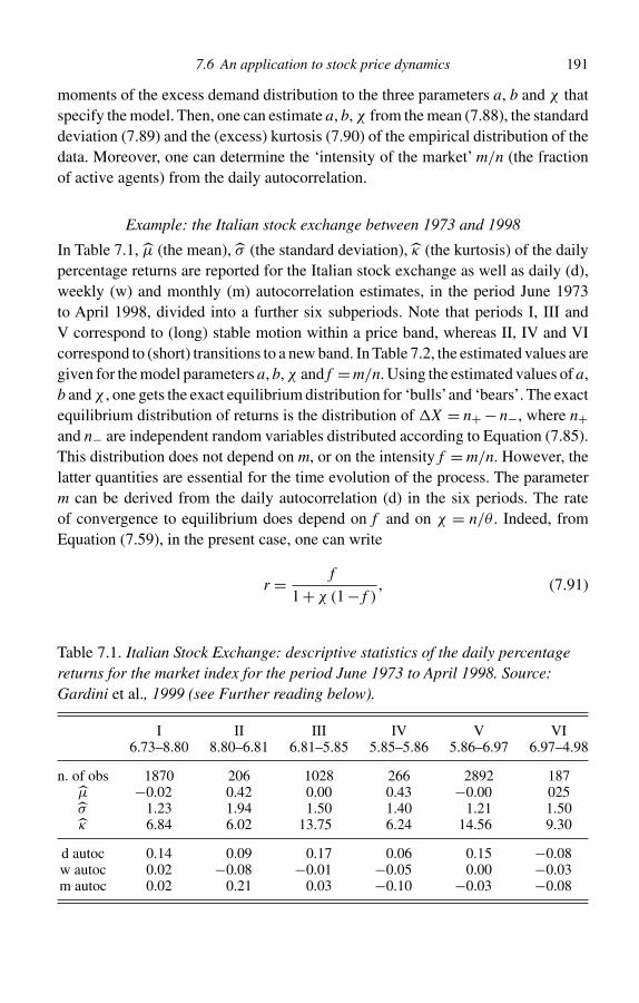
7.6 An application to stock price dynamics 191
moments of the excess demand distribution to the three parameters a, b and χ thatspecify the model. Then, one can estimate a, b, χ from the mean (7.88), the standarddeviation (7.89) and the (excess) kurtosis (7.90) of the empirical distribution of thedata. Moreover, one can determine the ‘intensity of the market’ m/n (the fractionof active agents) from the daily autocorrelation.
Example: the Italian stock exchange between 1973 and 1998
In Table 7.1, µ (the mean), σ (the standard deviation), κ (the kurtosis) of the dailypercentage returns are reported for the Italian stock exchange as well as daily (d),weekly (w) and monthly (m) autocorrelation estimates, in the period June 1973to April 1998, divided into a further six subperiods. Note that periods I, III andV correspond to (long) stable motion within a price band, whereas II, IV and VIcorrespond to (short) transitions to a new band. In Table 7.2, the estimated values aregiven for the model parameters a, b, χ and f = m/n. Using the estimated values of a,b and χ , one gets the exact equilibrium distribution for ‘bulls’and ‘bears’. The exactequilibrium distribution of returns is the distribution of X = n+ − n−, where n+and n− are independent random variables distributed according to Equation (7.85).This distribution does not depend on m, or on the intensity f = m/n. However, thelatter quantities are essential for the time evolution of the process. The parameterm can be derived from the daily autocorrelation (d) in the six periods. The rateof convergence to equilibrium does depend on f and on χ = n/θ . Indeed, fromEquation (7.59), in the present case, one can write
r = f
1 +χ (1 − f ), (7.91)
Table 7.1. Italian Stock Exchange: descriptive statistics of the daily percentagereturns for the market index for the period June 1973 to April 1998. Source:Gardini et al., 1999 (see Further reading below).
I II III IV V VI6.73–8.80 8.80–6.81 6.81–5.85 5.85–5.86 5.86–6.97 6.97–4.98
n. of obs 1870 206 1028 266 2892 187µ −0.02 0.42 0.00 0.43 −0.00 025σ 1.23 1.94 1.50 1.40 1.21 1.50κ 6.84 6.02 13.75 6.24 14.56 9.30
d autoc 0.14 0.09 0.17 0.06 0.15 −0.08w autoc 0.02 −0.08 −0.01 −0.05 0.00 −0.03m autoc 0.02 0.21 0.03 −0.10 −0.03 −0.08
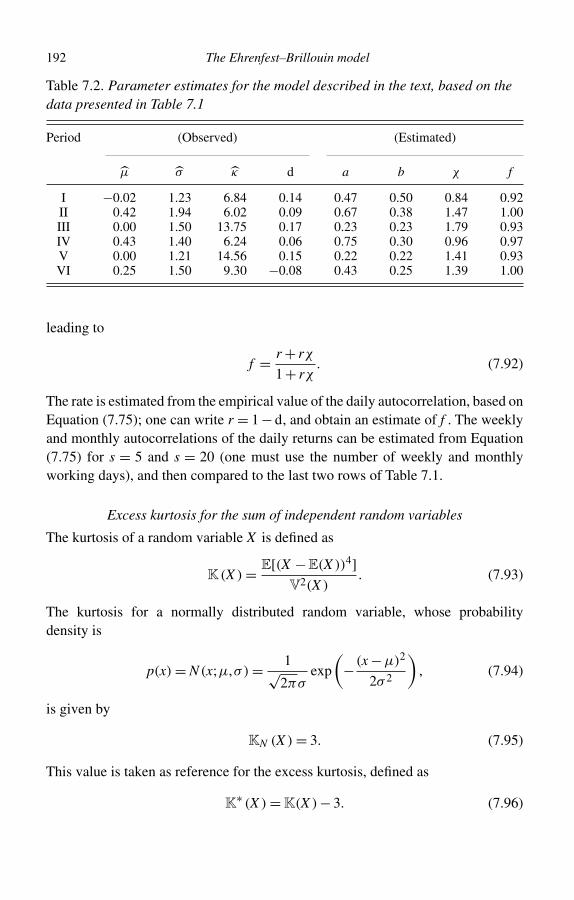
192 The Ehrenfest–Brillouin model
Table 7.2. Parameter estimates for the model described in the text, based on thedata presented in Table 7.1
Period (Observed) (Estimated)
µ σ κ d a b χ f
I −0.02 1.23 6.84 0.14 0.47 0.50 0.84 0.92II 0.42 1.94 6.02 0.09 0.67 0.38 1.47 1.00III 0.00 1.50 13.75 0.17 0.23 0.23 1.79 0.93IV 0.43 1.40 6.24 0.06 0.75 0.30 0.96 0.97V 0.00 1.21 14.56 0.15 0.22 0.22 1.41 0.93VI 0.25 1.50 9.30 −0.08 0.43 0.25 1.39 1.00
leading to
f = r + rχ
1 + rχ. (7.92)
The rate is estimated from the empirical value of the daily autocorrelation, based onEquation (7.75); one can write r = 1 − d, and obtain an estimate of f . The weeklyand monthly autocorrelations of the daily returns can be estimated from Equation(7.75) for s = 5 and s = 20 (one must use the number of weekly and monthlyworking days), and then compared to the last two rows of Table 7.1.
Excess kurtosis for the sum of independent random variables
The kurtosis of a random variable X is defined as
K(X ) = E[(X −E(X ))4]V2(X )
. (7.93)
The kurtosis for a normally distributed random variable, whose probabilitydensity is
p(x) = N (x;µ,σ) = 1√2πσ
exp
(−(x −µ)2
2σ 2
), (7.94)
is given by
KN (X ) = 3. (7.95)
This value is taken as reference for the excess kurtosis, defined as
K∗ (X ) = K(X )− 3. (7.96)
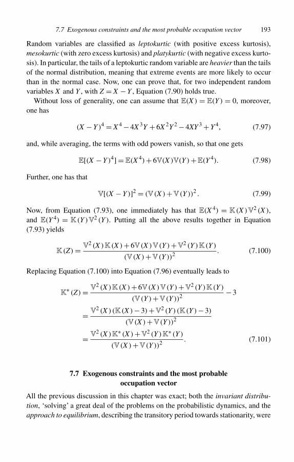
7.7 Exogenous constraints and the most probable occupation vector 193
Random variables are classified as leptokurtic (with positive excess kurtosis),mesokurtic (with zero excess kurtosis) and platykurtic (with negative excess kurto-sis). In particular, the tails of a leptokurtic random variable are heavier than the tailsof the normal distribution, meaning that extreme events are more likely to occurthan in the normal case. Now, one can prove that, for two independent randomvariables X and Y , with Z = X − Y , Equation (7.90) holds true.
Without loss of generality, one can assume that E(X ) = E(Y ) = 0, moreover,one has
(X − Y )4 = X 4 − 4X 3Y + 6X 2Y 2 − 4XY 3 + Y 4, (7.97)
and, while averaging, the terms with odd powers vanish, so that one gets
E[(X − Y )4] = E(X 4)+ 6V(X )V(Y )+E(Y 4). (7.98)
Further, one has that
V[(X − Y )]2 = (V(X )+V(Y ))2 . (7.99)
Now, from Equation (7.93), one immediately has that E(X 4) = K(X )V2 (X ),and E(Y 4) = K(Y )V2 (Y ). Putting all the above results together in Equation(7.93) yields
K(Z) = V2 (X )K(X )+ 6V(X )V(Y )+V2 (Y )K(Y )
(V(X )+V(Y ))2. (7.100)
Replacing Equation (7.100) into Equation (7.96) eventually leads to
K∗ (Z) = V2 (X )K(X )+ 6V(X )V(Y )+V2 (Y )K(Y )
(V(Y )+V(Y ))2− 3
= V2 (X )(K(X )− 3)+V2 (Y )(K(Y )− 3)
(V(X )+V(Y ))2
= V2 (X )K∗ (X )+V2 (Y )K∗ (Y )
(V(X )+V(Y ))2. (7.101)
7.7 Exogenous constraints and the most probableoccupation vector
All the previous discussion in this chapter was exact; both the invariant distribu-tion, ‘solving’ a great deal of the problems on the probabilistic dynamics, and theapproach to equilibrium, describing the transitory period towards stationarity, were
194 The Ehrenfest–Brillouin model
studied without approximations. This was possible because there were no exter-nal constraints to the motion of the system. A counterexample immediately comesfrom physics, for which the original Ehrenfest–Brillouin model was developed.Suppose that two particles collide, and that their final states are different from theinitial ones. The transition from the occupation state n to the occupation state nkl
ijis associated with the events D1 = i,D2 = j, representing the initial categories ofthe two selected particles, and C1 = k,C2 = l, representing the final categories ofthe colliding particles. Now, further assume that the collision is elastic, meaningthat the total energy of the two particles is the same before and after the collision.In other words, the transition can occur only if
ε(i)+ ε(j) = ε(l)+ ε(k), (7.102)
where ε(i) denotes the energy of a particle in the ith category, otherwise it isforbidden. In this case, it is useful to call the categories cells and divide the g cellsinto energy levels, grouping cells of equal energy. The parameters of the systemare n, the number of particles, and the set {gi,εi}i=1,...,d , where g =∑d
i=1 gi is thedecomposition of the g cells according to their energy. If cells are re-ordered withrespect to their energy in the following way (1, . . . ,g1,g1 +1, . . . ,g1 +g2,g1 +g2 +1, . . . ,
∑di=1 gi), with g0 = 0, the variable
Ni =∑i
k=1 gk∑j=1+∑i
k=1 gk−1
nj (7.103)
represents the occupation number of a level. The level-occupation vector N =(N1, . . . ,Nd ) is the so-called macrostate of the system, whereas the original cell-occupation vector (with cells numbered from 1 to g, as usual) n = (n1, . . . ,ng) is themicrostate of the system. The same procedure can be used for the initial weights,leading to
βi =∑i
k=1 gk∑j=1+∑i
k=1 gk−1
αj. (7.104)
If the system starts from a given microstate n and the energy is conserved, withunary moves, it cannot leave the initial macrostate N. On the contrary, binary movescan mimic elastic collisions, and the transition probability P(nkl
ij |n) still has the formof Equation (7.33), with a slight modification due to the existence of forbidden tran-sitions. In fact, the destruction term is given by the usual term 2(ni/n)[nj/(n − 1)]for i �= j, or by (ni/n)[(ni − 1)/(n − 1)] for i = j; if creation concerns cellsnot involved in the previous destructions, the creation term is proportional to
7.7 Exogenous constraints and the most probable occupation vector 195
2(αk +nk)(αl +nl) for l �= k, or to (αk +nk)(αk +nk +1) for l = k. These cumber-some notes are useful in order to write a program simulating the dynamics: at anystage of the move, one must use the current occupation number, possibly modifiedby previous partial moves. In order to normalize the creation probability, one mustconsider all final states reachable from nij adding two particles whose total energyis ε(l)+ ε(k) = ε(i)+ ε(j). Defining the term
Q(nklij |nij) = (2 − δlk)(αk + n′
k)(αl + n′l + δlk), (7.105)
where n′k and n′
l are the occupation numbers of nij, then one has
P(nklij |nij) = Q(nkl
ij |nij)∑k ′,l′ Q(nk ′l′
ij |nij), (7.106)
and, finally, the transition probability for the binary move is
P(nklij |n) = P(nij|n)P(nkl
ij |nij)
= (2 − δij)ni
n
nj − δij
n − 1
Q(nklij |nij)
Dδ[ε(l)+ ε(k)− (ε(i)+ ε(j))], (7.107)
where
D =∑k ′,l′
Q(nk ′l′ij |nij), (7.108)
and the sum is on the set
A(n, i, j) = {k ′, l′ : ε(l′)+ ε(k ′) = ε(i)+ ε(j)}. (7.109)
Therefore, not all the ‘first neighbours’ of the initial microstate n can be reachedin a single step, as the motion is confined to the so-called constant energy surface.Nevertheless, it is remarkable that, if P(nkl
ij |n) > 0, then also the inverse transition
is possible, that is P(n|nklij ) > 0. This is called microscopic reversibility. If one
considers all the states reachable from the initial state Y0 = n(0) by means ofrepeated applications of the transition probability (7.107), for all these states Yt =n(t), one finds that
∑gj=1 nj(t)ε(j) = ∑g
j=1 nj(0)ε(j) = E(n(0)) is a constant ofmotion. One can assume that all the states compatible with the constraint, i.e. theenergy surface or energy shell {n :
∑gj=1 njε(j) = E(n(0))}, can be reached by
means of binary collisions (if this is not the case, in principle, nothing preventsintroduction of m-ary collisions). In any case, the energy surface is a subset of theunconstrained state space Sn
g , which strongly depends on the values {gi,εi}i=1,2,...,d .Therefore, the transition matrix (7.107) rules a multidimensional random walk onthe energy surface which is an irreducible and aperiodic Markov chain.
196 The Ehrenfest–Brillouin model
In order to discuss the inverse transition, one can start from
nklij = n + k + l − i − j, (7.110)
where k, l, i and j indicate vectors which are zero everywhere except for thepositions k, l, i and j, respectively, where they are equal to 1. Now, consider thepath D1 = l,D2 = k, leading to nij = n−i − j, and the path C1 = j,C2 = i, leadingto n. Then, one has
P(nij|nklij ) = (2 − δlk)
nk
n
nl − δlk
n − 1, (7.111)
whereas
P(nijij|nij) = Q(nij
ij|nij)
D, (7.112)
where nijij = n and the denominator D coincides with the one in Equation (7.107).
In words, any path connecting n to nklij passes through the intermediate state nij
in both directions. In both cases the destructions end in nij, which is the startingstate for creations, all constrained to belong to the set A(n, i, j). Note that if onesets nkl
ij = n′, then nij = n′kl , and A(n,i, j) = A′(n′,k, l), as ε(l)+ ε(k) = ε(i)+ ε(j).
Given that the multiplicity factors are equal, one gets from Equation (7.107) andfrom the previous discussion
P(nklij |n)
P(n|nklij )
= ninj(αk + nk)(αl + nl)
(nk + 1)(nl + 1)(αi + ni − 1)(αj + nj − 1), (7.113)
for the case i �= j �= k �= l. Indeed, there exists a probability distribution whichsatisfies the detailed balance conditions, such that
π(nklij )
π(n)= P(nkl
ij |n)
P(n|nklij )
, (7.114)
where the right-hand side is given by Equation (7.113), and it is the following:
π(n) ∝g∏
j=1
α[nj]j
nj! . (7.115)
It is the usual generalized Pólya distribution now restricted to (or conditional on)all the states belonging to the energy surface. Note that one can check that Equation(7.115) works for all the possible cases, including those situations in which initialand final cells coincide. This is straightforward but boring.
7.7 Exogenous constraints and the most probable occupation vector 197
These last equations can be compared to the examples discussed at the beginningof the chapter. If ∀j, one has αj = 1 (the Bose–Einstein case), then one finds π(nkl
ij )=π(n) and one gets the uniform distribution restricted to the energy shell; if ∀j,αj = −1 (the Fermi–Dirac case), then one has π(nkl
ij ) = π(n) for all n : ni ∈ {0,1};finally, the case in which ∀j, one has αj → ∞ (the Maxwell–Boltzmann case) yields
π(n) ∝(∏g
j=1 nj!)−1
, which is uniform on all the allowed individual descriptions.
In other words, what was previously written in the abstract unconstrained case hereis valid, but within the energy shell. Further note that these results were obtainedwithout having a detailed description of the energy shell.
In all the three cases described above, all the parameters αj have the same value(all the cells are on a par, if allowed by the energy constraint); therefore, it is usefulto introduce the new parameter c = 1/αj. The creation factor αj + nj becomesproportional to 1 + cnj = c[(1/c)+ nj], and the three statistics relevant in physicsare obtained for c = 0,±1. For the Markov chain of macrostates N, the creationfactor becomes gi + cNi = c[(gi/c) + Ni]. From Equation (7.115), the invariantweight (to be normalized) of a macrostate is given by
W (N) =d∏
i=1
cNi(gi/c)[Ni]
Ni! , (7.116)
which becomes the usual weight for macrostates in statistical mechanics:
WBE(N) =d∏
i=1
gi[Ni]
Ni! =d∏
i=1
(gi + Ni − 1
Ni
), (7.117)
for c = 1 (Bose–Einstein case),
WFD(N) =d∏
i=1
gi[Ni]Ni! =
d∏i=1
(gi
Ni
), (7.118)
for c = −1 (Fermi–Dirac case) and
WMB(N) =d∏
i=1
giNi
Ni! , (7.119)
for c = 0 (Maxwell–Boltzmann case).In the unconstrained case, it is possible to eliminate the multivariate equilib-
rium distribution by marginalizing on a single category, and then obtain expected
198 The Ehrenfest–Brillouin model
values for the multivariate distribution; on the contrary, in the constrained case, theinitial symmetry of categories is broken by the energy function, and the marginalchain for a single category is very complicated. The only way to extract a uni-variate distribution from Equation (7.116) was envisaged by Boltzmann for thefirst time: it is the method of the most probable macrostate. In physics, the reasonto maximize the probability of the macrostate given in Equation (7.116) insteadof the microstate probability (7.115) is due to the assumed uniform distributionson the underlying microstates. Moreover, in physics, macrostates are obtained bymerging many energy levels, in order to obtain large values of Ni and gi so thatStirling’s approximation for factorials can be used. However, it is possible to use abetter procedure than applying Stirling’s approximation as one knows that Equation(7.116) is exact. The maximum of ln W (N) with the constraints
∑di=1 Ni = N = n
and∑d
i=1 Niεi = E is obtained by introducing Lagrange multipliers β, ν and byrequiring that (ln W (N) − βE+ νN ) = 0 (see also Section 5.3.8). The varia-tion is discrete. Considering the ith level, assume that Ni becomes Ni ± 1, so that Ei = ±εi and Ni = ±1. Now define W (Ni) as
W (Ni) = cNi(gi/c)[Ni]
Ni! ; (7.120)
considering that ln W (N) =∑di=1 ln W (Ni) one can calculate the variation of the
weight for a level if Ni becomes Ni ± 1 using (7.116):
+ ln W (Ni) = lnW (Ni + 1)
W (Ni)= ln
c(gi/c + Ni)
Ni + 1= ln
gi + cNi
Ni + 1, (7.121)
and
− ln W (Ni) = lnW (Ni − 1)
W (Ni)= ln
Ni
gi + c(Ni − 1)= − ln
gi + c(Ni − 1)
Ni.
(7.122)
Note that the term Ni + 1 in Equation (7.121) allows an accommodation in anempty cell, whereas the term Ni in Equation (7.122) forbids a destruction in anempty cell. These terms are important when Ni is small. But all this procedure isintended for macrostates where Ni � 1. In this case + ln W (Ni) and − ln W (Ni)
become equal in absolute value, Ni can be treated as a continuous variable and onecan write
d
dNiln W (Ni) = ln
gi + cNi
Ni= βεi − ν, (7.123)
7.7 Exogenous constraints and the most probable occupation vector 199
and deduce a simple analytical formula for the solution. If there exists a macrostateN∗ such that
ln(gi + cN ∗
i )
N ∗i
= βεi − ν, (7.124)
that is
N ∗i = gi
exp[βεi − ν]− c, (7.125)
then it is the most probable macrostate, which for c = 1,−1,0 represents the Bose–Einstein, the Fermi–Dirac and the Maxwell–Boltzmann case, respectively. Thetwo new parameters β,ν must be chosen so that
∑di=1 N ∗
i = N and∑d
i=1 N ∗i εi = E.
Returning to the exact formulae (7.121) and (7.122), considering the transitionP(Nkl
ij |N), the variation of ln W (N) is just ln W (Nklij ) − ln W (N), which contains
four terms if all levels are different, leading to
ln W (Nklij )− ln W (N)
= + ln W (Nk)+ + ln W (Nl)+ − ln W (Ni)+ − ln W (Nj)
= lnNi
gi + c(Ni − 1)
Nj
gj + c(Nj − 1)
gk + cNk
Nk + 1
gl + cNl
Nl + 1
= lnP(Nkl
ij |N)
P(N|Nklij )
= lnπ(Nkl
ij )
π(N), (7.126)
where the last equalities are a direct consequence of Equation (7.114) applied tomacrostates. In the limit of large occupation numbers, if the starting N is N∗, andapplying Equation (7.123), one finds that
ln W (N∗) = β(εk + εl − εi − εj) = 0, (7.127)
if Nklij has the same energy as N∗. This means that the probability is ‘flat’around N∗,
as all its first neighbours have nearly the same probability. In words, starting fromN∗, and considering any transition which satisfies the energy constraint (that is suchthat εk +εl = εi +εj), the final vector is still in the region of maximum probability.For macroscopic physical systems, where n is roughly 1023, the assumption ofstatistical mechanics is that the region of motion is overwhelmingly concentratedaround N∗, which then summarizes all the underlying dynamics and, at least, allequilibrium properties. Quite surprisingly, a formula similar to Equation (7.125)also holds true for small values of n. In fact, considering the expected flux
φklij =
∑N
P(Nklij |N)P(N), (7.128)
200 The Ehrenfest–Brillouin model
which is the probability that a transition i, j → k, l occurs whatever the initial stateN may be, and the reversed flux
φijkl =
∑N
P(Nijkl |N)P(N), (7.129)
then assuming that the two fluxes are equal, one has that φklij /φ
ijkl = 1. Now, one can
write
φklij /φ
ijkl = E[NiNj(gk + cNk)(gl + cNl)]
E[NkNl(gi + cNi)(gj + cNj)] . (7.130)
If one can approximate the expectation of the product with the product ofexpectations, then from φkl
ij /φijkl = 1 one gets
lnE[Ni]
gi + cE[Ni]E[Nj]
gj + cE[Nj]gk + cE[Nk ]
E[Nk ]gl + cE[Nl]
E[Nl] = 0; (7.131)
in other words, if for any energy level ln[E[Ni]/(gi + cE[Ni])] = ν −βεi then forany conservative collision the two fluxes equalize. Then Equation (7.125) can bere-written for expected values also
E[Ni] = gi
exp[βεi − ν]− c. (7.132)
Although both Equations (7.132) and (7.125) are approximate, in some applications(7.125) could be meaningless, whereas Equation (7.132) is always meaningful. Forinstance, consider a system with gi = 1 for all the values of i. This is strange inphysics, where gi is an increasing function of i, but it can be the case in economicsor in other fields. Then Equation (7.125) could still apply, because it was derivedonly for Ni � 1, while the usual Stirling’s approximation also needs gi � 1. In thisparticular case, macrostates and microstates do coincide. Further assume that c = 1.One knows from Equation (7.14) that the equilibrium distribution is flat, that is allthe states are equiprobable. Hence there is no N∗ at all! On the contrary, and thisis confirmed by computer simulation, E[Ni] can be derived from the time averageof occupation numbers for the ith level as time goes by, and an almost qualitativeagreement with Equation (7.132) is easily obtained even for n < 100. Note that ifthere exists N∗ such that π(N∗) ≈ 1, then E[Ni] =∑Niπ(N) ≈ N ∗
i , but E[Ni] alsoexists when there is no predominant macrostate N∗.
Finally, in order to justify the assumption leading from Equation (7.130) toEquation (7.131), note that if g random variables satisfy the constraint
∑g1 Xi = n,
then V(∑g
1 Xi) =∑g1 V(Xi) +∑j �=i C(Xi,Xj) = 0 (see also Section 5.4). Even if
all the variables Xi are not equidistributed, one finds that Equation (5.94) gives the
7.9 Summary 201
order of magnitude for the Bravais–Pearson correlation which is
ρ(Xi,Xj) = − 1
g − 1. (7.133)
Given that in any concrete case, the number g of levels involved in the dynamicsis far larger than n, the correlation between the occupation numbers is negligible,and the corresponding approximation works fairly well.
7.8 Exercises
7.1 Consider the aperiodic Ehrenfest urn discussed at length in Chapter 6, set n = 4and further consider a double selection, followed by a double independentcreation. A transition path is D1, D2, C1, C2 where D1,D2 are conditionedon the starting state k = 0, . . . ,4, whereas C1, C2 are independent. Therefore,one has P(C1,C2) = 1/4 uniformly on all the four possibilities. Show that thetransition matrix with m = 2 (binary moves) is different from the square of thematrix with m = 1 given by Equation (6.30).
7.2 Write a Monte Carlo program for the Ehrenfest–Brillouin model with unarymoves. In the dichotomous case, compare the results for α1 = α2 = 10 andα1 = α2 = 1/2.
7.9 Summary
In the general case of m-ary moves, the Ehrenfest–Brillouin model is a Markovchain specified by the transition probability (7.53) and by the initial occupationvector n(0) (or, in a more abstract way, by the initial probability distribution P(0)).It describes the probabilistic dynamics of n objects jumping within g categories.The transition probability factorizes into ‘random’ destruction terms, as in the caseof the Ehrenfest urn model, and creation terms following the generalized Pólyamechanism, as in the case of Brillouin’s model. Each term is computed accordingto the current occupation state of the system with destructions preceding creations.For instance, in the case of binary moves, first an object is randomly selected fromall the n objects and removed, then a second object is removed after being extractedfrom the remaining n−1 objects. Then the objects accommodate one after the otheraccording to the Pólya mechanism. Before the first accommodation n − 2 objectsare left in the system and before the second accommodation there are n−1 objects.
If no exogenous constraint is imposed on the ‘motion’ of the chain, then it ispossible to marginalize the multivariate Markov chain and follow the evolution ofa single category as in Equation (7.54). Otherwise, in the presence of constraints,the time evolution of the Ehrenfest–Brillouin Markov chain is limited to the subsetof all the possible occupation states satisfying the constraints. In the unconstrained
202 The Ehrenfest–Brillouin model
cases, the invariant distribution of this model is a multivariate Pólya distribution,whereas in the constrained cases, it is still a Pólya but re-normalized over the subsetof accessible states. In all the cases, this is also an equilibrium distribution.
The Ehrenfest–Brillouin model is remarkably general and flexible and it encom-passes many popular models used in physics, economics and finance. In particular,as invariant and equilibrium distributions one recovers the popular Bose–Einstein,Fermi–Dirac and Maxwell–Boltzmann distributions of statistical physics as wellas the equilibrium distribution for the celebrated Kirman’s ant model. Moreover,all the limits of the Pólya distribution described in Chapter 5 apply.
Further reading
There are many introductory books on statistical mechanics. Jancel’s book is aclassical one with emphasis on foundational problems:
R. Jancel, Foundations of Classical and Quantum Statistical Mechanics, Pergamon Press,Oxford, UK (1969).
The seminal paper by Brillouin is listed in further reading for Chapter 4, whereasthe encyclopaedia article written by P. and T. Ehrenfest is listed in Chapter 6.The Ehrenfest–Brillouin model was introduced in a series of papers written byD. Costantini and U. Garibaldi with applications to statistical physics in mind.
D. Costantini and U. Garibaldi, A Probabilistic Foundation of Elementary Particle Statistics.Part I, Studies in History and Philosophy of Modern Physics, 28, 483–506 (1997).
D. Costantini and U. Garibaldi, A Probabilistic Foundation of Elementary Particle Statistics.Part II, Studies in History and Philosophy of Modern Physics, 29, 37–59 (1998).
The most relevant paper, published by Synthese, is listed in further reading forChapter 4.
A. Kirman’s original paper including his ‘ant model’ was published in 1993:
A. Kirman, Ants, Rationality, and Recruitment, The Quarterly Journal of Economics, 108,137–156 (1993).
The data in Section 7.6 are taken from a paper by Gardini et al.
A. Gardini, G. Cavaliere and M. Costa, A New Approach to Stock Price Modeling andForecasting, Journal of the Italian Statistical Society, 8, 25–47 (1999).
whose results were later updated in
A. Gardini, G. Cavaliere and M. Costa, Fundamentals and Asset Price Dynamics, StatisticalMethods & Applications, 12, 211–226 (2003).
Note that market daily data are freely available from several websites. The modelof Section 7.6 was introduced in

7.9 Summary 203
U. Garibaldi, M.A. Penco and P. Viarengo, An Exact Physical Approach to MarketParticipation Models, in R. Cowan and N. Jonard (eds.), Heterogeneous Agents, Interac-tions and Economic Performance, Lecture Notes in Economics and Mathematical Systems,521, 91–103, Springer, Berlin (2003).
Variations on the theme of the Ehrenfest–Brillouin model were used byG. Bottazzi et al.
G. Bottazzi, G. Fagiolo, G. Dosi and A. Secchi, Modeling Industrial Evolution inGeographical Space, Journal of Economic Geography, 7, 651–672 (2007).
G. Bottazzi, G. Fagiolo, G. Dosi and A. Secchi, Sectoral and Geographical Specificities inthe Spatial Structure of Economic Activities, Structural Change and Economic Dynamics,19, 189–202 (2008).
to analyze industrial evolution in geographical space both theoretically andempirically.
8
Applications to stylized models in economics
This chapter is devoted to three models where n objects move within g categoriesaccording to some prescribed transition probabilities. The natural way of presentingthese models is in terms of transition probabilities over occupation states Y = n.Individual descriptions, occupation vectors as well as partition vectors can be givenan interpretation in terms of economic variables. The three models are irreducibleand aperiodic Markov chains; therefore they have a unique invariant distributionwhich is also the equilibrium distribution.
After reading this chapter you should be able to:
• intepret the random vectors discussed in the previous chapters of the book interms of economic variables;
• understand the role of the methods discussed in Section 5.3.8 and in Chapter6, in order to derive simple analytical results for comparison with Monte Carlosimulations and real data;
• understand three simple stylized economic models.
8.1 A model for random coin exchange
Consider g agents and n coins to be distributed among them. This problem wasconsidered in the example in Section 2.3.2 as well as in the exercises of Chapter 6.In this problem, knowing that the ith coin belongs to the jth agent is a marginalindividual description and the vector (random) variable X = (X1 = x1, . . . ,Xn =xn), where xi ∈ {1, . . . ,g} gives full information on the position of the coins. Thefrequency (random) vector Y = (Y1 = n1, . . . ,Yg = ng) contains information onthe number of coins belonging to each agent, with the constraint that
∑gi=1 ni = n.
Finally, the numbers of agents with zero coin, one coin, etc. are included in thepartition (random) vector Z = (Z0 = z0, . . . ,Zn = zn), with the two constraints that∑n
i=0 zi = g and∑n
i=0 izi = n. Usually, one considers a random interaction betweentwo agents who randomly meet; one of them is a loser with probability 1/2 andthe other is a winner. The winner receives a coin from the loser. If the loser has
204
8.1 A model for random coin exchange 205
no coins left, the move is not considered. After a little thought, one can avoid theproblem of empty steps considering the following description of the game. Givenan initial frequency vector n0:
1. at each step a loser is selected by chance from all the agents with at least onecoin;
2. the loser gives one of his/her coins to a winner randomly selected from all theagents.
Note that, with this mechanism, the winner may well coincide with the loser. Asfurther discussed in Exercises 8.1 and 8.2 below, this game can be described by afinite Markov chain with the following transition probability
P(n′|n) = 1 − δni ,0
g − z0(n)
1
g, (8.1)
where
1. after the move, the frequency vector n′ differs from n at most by the change ofposition of one coin. In other words if agent i is selected as a loser and agentj �= i as a winner, one has that n′
i = ni − 1 and n′j = nj + 1 and n′ = nj
i with adestruction in category i followed by a creation in category j;
2. the numerator 1 − δni ,0 means that the loser is selected from the agents with atleast one coin;
3. the denominator g − z0(n) is the number of agents with at least one coin, asz0(n) is the number of agents with no coins;
4. the term 1/g represents the probability of selecting one of the agents at random;5. the selections of the loser and of the winner are independent and the transition
probability (8.1) is the product of the probability of selecting a loser and theprobability of selecting a winner.
Exercises 8.1 and 8.2 below show how to determine the invariant probability dis-tribution for this finite Markov chain using the eigenvector method as well as theMonte Carlo method. However, both methods become cumbersome for a largestate space and in this particular case, the state space is a rapidly growing functionof both g and n. For instance, for n = 20 coins and g = 10 agents, one alreadyhas more than ten million possible occupation states. Fortunately enough, for thisMarkov chain, the invariant distribution can be determined by imposing the detailedbalance conditions.
8.1.1 The invariant distribution
Consider two subsequent states (n1, . . . ,ni, . . . ,nj, . . . ,ng) and (n1, . . . ,ni −1, . . . ,nj + 1, . . . ,ng) with ni > 0 and i �= j. If one tries to apply detailed balance,
206 Applications to stylized models in economics
one has that the ‘direct flux’ is given by
π(n)P(nji|n) = π(n)
1
g − z0(n)
1
g, (8.2)
whereas the ‘inverse flux’ is
π(nji)P(n|nj
i) = π(nji)
1
g − z0(nji)
1
g; (8.3)
equating the two fluxes leads to
π(n)1
g − z0(n)
1
g= π(nj
i)1
g − z0(nji)
1
g, (8.4)
which is always satisfied if
π(n) = C(g − z0(n)), (8.5)
where C is a suitable normalization constant. In other words, the invariant prob-ability distribution for this model is proportional to the number of agents with atleast one coin in their pocket. If n � g, and starting from a uniform distributionof coins among agents, then the number of agents without coins is z0 = 0, and itis very unlikely to see z0 > 0 as time goes by. In other words, a very long time isneeded to see a state in which some agent remains without coins. Setting z0 = 0 inEquation (8.5) leads to a π(n) uniform on all agent descriptions whose number is
W (g,n) =(
n + g − 1
n
). (8.6)
Therefore, if g � 1, one finds that the marginal description of an agent is thegeometric distribution discussed in Section 5.3.2. Given the assumed uniformity, thesame result can be obtained using the Lagrange multiplier method for the partitionvector. Note that the mode of the geometric distribution is just z0, that is the mostoccupied state is expected to be z0 contrary to the initial assumption! Indeed, it willbe seen that for n and g finite, one can get coin distributions which significantlydiffer from the asymptotic geometric case.
Returning to the invariant distribution (8.5), in order to determine the normaliza-tion constant C, one notices that the total number of occupation states is given byEquation (8.6) as already discussed many times. The number of agent descriptionswith k fixed agents possessing one coin at least (while all the other n−k agents willremain with zero coins) is given by the ways of allocating n − k coins to k agents:(
n − k + k − 1
n − k
)=(
n − 1
n − k
)=(
n − 1
k − 1
), (8.7)
8.1 A model for random coin exchange 207
in fact, the first k coins are used as placeholders, and there are n!/(k!(n−k)!) waysto choose these k agents. Therefore the number of agent descriptions with k agentspossessing one coin at least is
W (k,g,n) =(
n
k
)(n − 1
n − k
). (8.8)
For instance, in the case of maximum coin concentration (k = 1), Equation (8.8)gives W (1,g,n) = n, as any agent can be the richest. Now, the total number ofagent descriptions is just the sum of all the descriptions with k agents with at leastone coin in their pockets (all the other agents being without coins); in other words,one has
W (g,n) =(
n + g − 1
n
)=
g∑k=1
(n
k
)(n − 1
n − k
)=
g∑k=1
W (k,g,n); (8.9)
this equation represents the decomposition of the total number of states into allpossible values of k. Coming back to Equation (8.5), one can write the followingchain of equalities
1 =∑
n
π(n) = C∑
n
(g − z0(n)) = C∑
n
k(n)
= Cg∑
k=1
kW (k,g,n) = Cg∑
k=1
k
(n
k
)(n − 1
n − k
), (8.10)
so that one eventually finds
C =[ g∑
k=1
k
(n
k
)(n − 1
n − k
)]−1
. (8.11)
The fourth equality in Equation (8.10) is justified by the fact that W (k,g,n) is thenumber of terms with a given value of k(n).
8.1.2 The expected wealth distribution
The marginal method presented in Section 5.3.8 can be used to obtain the expectedwealth distribution (namely, the distributions of coins) in this case. The relevantrandom variable is the partition vector Z = (Z0 = z0, . . . ,Zn = zn) where z0 is thenumber of agents without coins, z1 is the number of agents with 1 coin, and so on,up to zn which gives the number of agents with n coins. As mentioned many times,
208 Applications to stylized models in economics
these numbers must satisfy the two following constraints:
n∑i=0
zi = g, (8.12)
andn∑
i=1
izi = n. (8.13)
As in Equation (5.72) of Section 5.3.8, thanks to agent symmetry, one has that
P(Z = z) = g!n∏
i=0
zi!P(Y = n) = g!
n∏i=0
zi!C(g − z0(n)). (8.14)
Using the approximate method of Lagrange multipliers in order to find the mostprobable vector is not easy in this case, but the exact marginalization method worksand, for each random variable Zi, one can determine its average value E(Zi).
As a consequence of Equations (5.74) and (5.75), the average number of agentswhose occupation number is equal to i is
E(Zi) = gP(n1 = i), (8.15)
as all the nis are equidistributed. The first step for deriving E(Zi) is studying theconditional average
E(Zi|k) = gP(n1 = i|k), (8.16)
whose meaning is the marginal wealth distribution of an agent conditioned to k =g − z0. From Equation (8.5), it is apparent that all agent descriptions with the samek have the same probability, and their number is W (k,g,n) given in Equation (8.8).Therefore, P(n1 = i|k) is given by the number of occupation vectors in which g −1agents share n− i coins divided by W (k,g,n). This calculation can be divided intothree parts. First, consider P(n1 = 0|k); one has:
P(n1 = 0|k) = W (k,g − 1,n)
W (k,g,n)=
(g − 1
k
)(n − 1
k − 1
)(
g
k
)(n − 1
k − 1
)
=
(g − 1
k
)(
g
k
) = (g − 1)!(g − 1 − k)!
(g − k)!g! = g − k
g, (8.17)
8.1 A model for random coin exchange 209
then, consider P(n1 = i|k) with k ≥ 2, and i > 0; as there are k −1 agents left withat least one coin, one has:
P(n1 = i|k) = W (k − 1,g − 1,n − i)
W (k,g,n)
=
(g − 1
k − 1
)(n − i − 1
k − 2
)(
g
k
)(n − 1
n − k
) = k
g
(n − i − 1
k − 2
)(
n − 1
k − 1
) ; (8.18)
note that the above formula is valid for n − i − 1 ≥ k − 2 and i = 1, . . . ,n − 1. Ifthese conditions are not satisfied, then P(n1 = i|k) = 0. Finally, for k = 1, one finds:
P(n1 = i|k = 1) = δi,n
g, (8.19)
for i > 0, as in this case all the coins are concentrated on a single agent. Eventually,from Equation (8.16) one finds
E(Z0|k) = g − kE(Zi|k > 1) = k
(n − i − 1
k − 2
)(
n − 1
k − 1
) , i = 1, . . . ,n − 1
E(Zi|k = 1) = δi,n, i = 1, . . . ,n;
(8.20)
and further E(Zi|k) = 0 for n− i−1 < k −2 and i = n. The average marginal wealthdistribution E(Zi) is related to the average marginal conditional wealth distributionE(Zi|k) by means of the following equation:
E(Zi) =g∑
k=0
P(k)E(Zi|k). (8.21)
Therefore, P(k) is still needed. However, this is immediately given by Equation(8.5), recalling that there are W (k,g,n) occupation vectors with the same value of k:
P(k) = CkW (k,g,n) = Ck
(g
k
)(n − 1
k − 1
). (8.22)
Note that one hasn∑
i=0
E(Zi)
g= 1; (8.23)
therefore, it is meaningful to compare E(Zi)/g to the histograms for the relativefrequency of agents with i coins in a Monte Carlo simulation of this model.
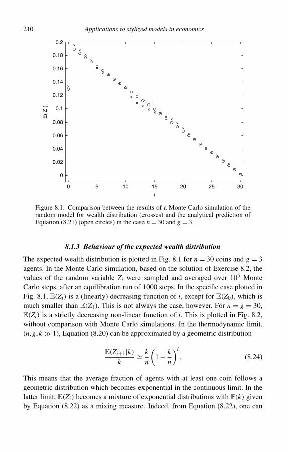
210 Applications to stylized models in economics
0 5 10 15 20 25 30
0
0.02
0.04
0.06
0.08
0.1
0.12
0.14
0.16
0.18
0.2
i
E(Z
i)
Figure 8.1. Comparison between the results of a Monte Carlo simulation of therandom model for wealth distribution (crosses) and the analytical prediction ofEquation (8.21) (open circles) in the case n = 30 and g = 3.
8.1.3 Behaviour of the expected wealth distribution
The expected wealth distribution is plotted in Fig. 8.1 for n = 30 coins and g = 3agents. In the Monte Carlo simulation, based on the solution of Exercise 8.2, thevalues of the random variable Zi were sampled and averaged over 105 MonteCarlo steps, after an equilibration run of 1000 steps. In the specific case plotted inFig. 8.1, E(Zi) is a (linearly) decreasing function of i, except for E(Z0), which ismuch smaller than E(Z1). This is not always the case, however. For n = g = 30,E(Zi) is a strictly decreasing non-linear function of i. This is plotted in Fig. 8.2,without comparison with Monte Carlo simulations. In the thermodynamic limit,(n,g,k � 1), Equation (8.20) can be approximated by a geometric distribution
E(Zi+1|k)
k k
n
(1 − k
n
)i
. (8.24)
This means that the average fraction of agents with at least one coin follows ageometric distribution which becomes exponential in the continuous limit. In thelatter limit, E(Zi) becomes a mixture of exponential distributions with P(k) givenby Equation (8.22) as a mixing measure. Indeed, from Equation (8.22), one can
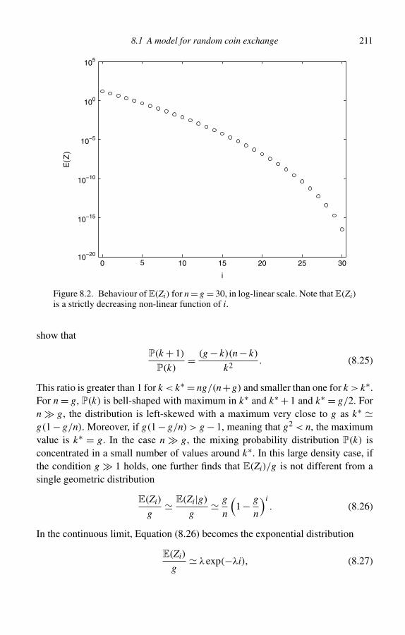
8.1 A model for random coin exchange 211
0 5 10 15 20 25 3010−20
10−15
10−10
10−5
100
105
i
E(Z
)
Figure 8.2. Behaviour of E(Zi) for n = g = 30, in log-linear scale. Note that E(Zi)is a strictly decreasing non-linear function of i.
show that
P(k + 1)
P(k)= (g − k)(n − k)
k2. (8.25)
This ratio is greater than 1 for k < k∗ = ng/(n+g) and smaller than one for k > k∗.For n = g, P(k) is bell-shaped with maximum in k∗ and k∗ + 1 and k∗ = g/2. Forn � g, the distribution is left-skewed with a maximum very close to g as k∗ g(1 − g/n). Moreover, if g(1 − g/n) > g − 1, meaning that g2 < n, the maximumvalue is k∗ = g. In the case n � g, the mixing probability distribution P(k) isconcentrated in a small number of values around k∗. In this large density case, ifthe condition g � 1 holds, one further finds that E(Zi)/g is not different from asingle geometric distribution
E(Zi)
g E(Zi|g)
g g
n
(1 − g
n
)i. (8.26)
In the continuous limit, Equation (8.26) becomes the exponential distribution
E(Zi)
g λexp(−λi), (8.27)
212 Applications to stylized models in economics
where λ = g/n. This final remark explains why simulations of this model in thecase n � g � 1 give an exponential wealth distribution.
8.2 The taxation–redistribution model
In the previous section, a stylized model for the redistribution of wealth was dis-cussed. In that model one coin out of n is taken from a randomly chosen agentwith at least one coin and redistributed to a randomly selected agent. Indebtednessis not possible. The model can be modified along the following lines. There arealways n coins to be distributed among g agents. A taxation is a step in which acoin is randomly taken out of n coins and a redistribution is a step in which thecoin is given to one of the g agents. In the language of Chapter 6, a taxation isequivalent to a destruction and a redistribution to a creation. As in the previousmodel, coins and agents do not disappear and the taxation–redistribution modelis conservative. This model considers only unary moves of the kind presented inFig. 6.1. Therefore, the initial state is n = (n1, . . . ,ni, . . . ,nj, . . . ,ng) and the final
state is nji = (n1, . . . ,ni −1, . . . ,nj +1, . . . ,ng). If a coin is randomly selected out of
n coins, the probability of selecting a coin belonging to agent i is ni/n. Therefore,in this model, agents are taxed proportionally to their wealth measured in termsof the number of coins in their pockets. The redistribution step is crucial as it canfavour agents with many coins (a rich gets richer mechanism) or agents with fewcoins (a taxation scheme leading to equality). This can be done by assuming thatthe probability of giving the coin taken from agent i to agent j is proportional towj +nj where nj is the number of coins in the pocket of agent j and wj is a suitableweight. Depending on the choice of wj, one can obtain very different equilibriumsituations. Based on the previous considerations, it is assumed that the transitionprobability is
P(nji|n) = ni
n
wj + nj − δi,j
w + n − 1, (8.28)
where w =∑gi=1 wi and the Kronecker symbol δi,j takes into account the case i = j.
If the condition wj �= 0 is satisfied, then also agents without coins can receive them.If all the agents are equivalent, one has wj = α uniformly, and w = gα = θ , so thatEquation (8.28) becomes
P(nji|n) = ni
n
α + nj − δi,j
θ + n − 1. (8.29)
This is the Ehrenfest–Brillouin model with unary moves discussed in Section 7.2,whose invariant and equilibrium distribution is the g-variate generalized Pólya
8.2 The taxation–redistribution model 213
distribution, given below for the convenience of the reader
π(n) = n!θ [n]
g∏i=1
α[ni]
ni! . (8.30)
In contrast to what is found in physics, here α is not limited to the values ±1 and∞. Indeed, the redistribution policy is characterized by the value of the parameterα. In parallel to physics, if α is small and positive, rich agents become richer, butfor α → ∞ the redistribution policy becomes random: any agent has the sameprobability of receiving the coin. Finally, the case α < 0 favours poor agents, but|α| is the maximum allowed wealth for each agent.
8.2.1 Marginal description and expected wealth distribution
As in the model described in the previous section, agents’ equivalence leads to asimple relationship between the joint probability distribution of partitions and theprobability of a given occupation vector. From Equations (5.72) and (8.30), one gets
P(Z = z) = g!∏ni=0 zi!P(Y = n) = g!∏n
i=0 zi!n!∏g
j=1 ni!g∏
j=1
α[ni]
θ [n]
= g!n!∏ni=0 zi!(i!)zi
g∏j=1
α[ni]
θ [n] , (8.31)
where, as usual, zi is the number of agents with i coins. In contrast to physics,where the constrained maximisation is necessary, the exact marginal method canbe used here. All the agents are characterized by the same weight α. Given thisequivalence, it is meaningful to focus on the behaviour of the random variableY = Y1 representing the number of coins of agent 1. If one begins from Yt = k, onecan define the following transition probabilities:
w(k,k + 1) = P(Yt+1 = k + 1|Yt = k) = n − k
n
α + k
θ + n − 1, (8.32)
meaning that a coin is randomly removed from one of the other n−k coins belongingto the other g − 1 agents and given to agent 1 according to the weight α and thenumber of coins k;
w(k,k − 1) = P(Yt+1 = k − 1|Yt = k) = k
n
θ −α + n − k
θ + n − 1, (8.33)
214 Applications to stylized models in economics
meaning that a coin is randomly removed from agent 1 and redistributed to one ofthe other agents according to the weight θ −α and the number of coins n − k; and
w(k,k) = P(Yt+1 = k|Yt = k) = 1 −w(k,k + 1)−w(k,k − 1), (8.34)
meaning that agent 1 is not affected by the move. These equations define a birth–death Markov chain corresponding to a random walk with semi-reflecting barriers.This chain was studied in detail in Section 7.5.3. However, the invariant (andequilibrium) distribution can be directly obtained by marginalizing Equation (8.30).This leads to the dichotomous Pólya distribution, as discussed in Section 5.3:
P(Y = k) = n!k!(n − k)!
α[k](θ −α)[n−k]
θ [n] . (8.35)
As a consequence of the equivalence of all agents, from Equations (5.74) and (5.75),one obtains
E(Zk) = gP(Y = k) = gn!
k!(n − k)!α[k](θ −α)[n−k]
θ [n] . (8.36)
Equation (8.36) gives the expected wealth distribution for the taxation–redistribution model. Following Section 5.5, in the continuous thermodynamiclimit, one can see that the equilibrium expected wealth distribution of the taxation–redistribution model is approximately described, for α > 0, by the gammadistribution of parameters α and n/αg.
8.2.2 Block taxation and the convergence to equilibrium
Consider the case in which taxation is done in a block: instead of extracting asingle coin from an agent at each step, m ≤ n coins are randomly taken fromvarious agents and then redistributed with the mechanism described above, that iswith a probability proportional to the residual number of coins and to an a-prioriweight. If n = (n1, . . . ,ng) is the initial occupation vector, m = (m1, . . . ,mg) (with∑g
i=1 mi = m) is the taxation vector and m′ = (m′1, . . . ,m′
g) (with∑g
i=1 m′i = m) is
the redistribution vector, one can write
n′ = n − m + m′. (8.37)
This is essentially the Ehrenfest–Brillouin model with m-ary moves studied inSection 7.5.3. The main results of that section are summarized below interpretedin the framework of the model. The block taxation–redistribution model still hasEquation (8.30) as its equilibrium distribution, as the block step is equivalent to msteps of the original taxation–redistribution model.
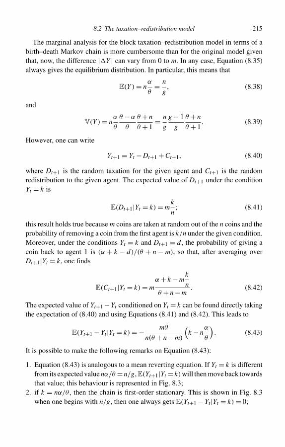
8.2 The taxation–redistribution model 215
The marginal analysis for the block taxation–redistribution model in terms of abirth–death Markov chain is more cumbersome than for the original model giventhat, now, the difference | Y | can vary from 0 to m. In any case, Equation (8.35)always gives the equilibrium distribution. In particular, this means that
E(Y ) = nα
θ= n
g, (8.38)
and
V(Y ) = nα
θ
θ −α
θ
θ + n
θ + 1= n
g
g − 1
g
θ + n
θ + 1. (8.39)
However, one can write
Yt+1 = Yt − Dt+1 + Ct+1, (8.40)
where Dt+1 is the random taxation for the given agent and Ct+1 is the randomredistribution to the given agent. The expected value of Dt+1 under the conditionYt = k is
E(Dt+1|Yt = k) = mk
n; (8.41)
this result holds true because m coins are taken at random out of the n coins and theprobability of removing a coin from the first agent is k/n under the given condition.Moreover, under the conditions Yt = k and Dt+1 = d , the probability of giving acoin back to agent 1 is (α + k − d)/(θ + n − m), so that, after averaging overDt+1|Yt = k, one finds
E(Ct+1|Yt = k) = mα + k − m
k
nθ + n − m
. (8.42)
The expected value of Yt+1 −Yt conditioned on Yt = k can be found directly takingthe expectation of (8.40) and using Equations (8.41) and (8.42). This leads to
E(Yt+1 − Yt|Yt = k) = − mθ
n(θ + n − m)
(k − n
α
θ
). (8.43)
It is possible to make the following remarks on Equation (8.43):
1. Equation (8.43) is analogous to a mean reverting equation. If Yt = k is differentfrom its expected value nα/θ = n/g, E(Yt+1|Yt = k)will then move back towardsthat value; this behaviour is represented in Fig. 8.3;
2. if k = nα/θ , then the chain is first-order stationary. This is shown in Fig. 8.3when one begins with n/g, then one always gets E(Yt+1 − Yt|Yt = k) = 0;
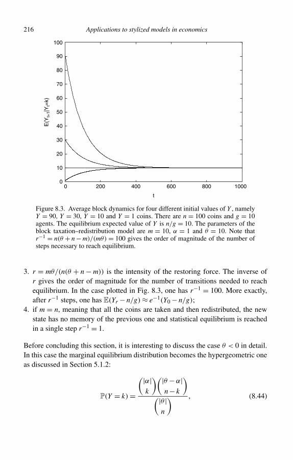
216 Applications to stylized models in economics
0 200 400 600 800 10000
10
20
30
40
50
60
70
80
90
100
t
E(Y
t+1|
Yt=
k)
Figure 8.3. Average block dynamics for four different initial values of Y , namelyY = 90, Y = 30, Y = 10 and Y = 1 coins. There are n = 100 coins and g = 10agents. The equilibrium expected value of Y is n/g = 10. The parameters of theblock taxation–redistribution model are m = 10, α = 1 and θ = 10. Note thatr−1 = n(θ + n − m)/(mθ) = 100 gives the order of magnitude of the number ofsteps necessary to reach equilibrium.
3. r = mθ/(n(θ + n − m)) is the intensity of the restoring force. The inverse ofr gives the order of magnitude for the number of transitions needed to reachequilibrium. In the case plotted in Fig. 8.3, one has r−1 = 100. More exactly,after r−1 steps, one has E(Yr − n/g) ≈ e−1(Y0 − n/g);
4. if m = n, meaning that all the coins are taken and then redistributed, the newstate has no memory of the previous one and statistical equilibrium is reachedin a single step r−1 = 1.
Before concluding this section, it is interesting to discuss the case θ < 0 in detail.In this case the marginal equilibrium distribution becomes the hypergeometric oneas discussed in Section 5.1.2:
P(Y = k) =
(|α|k
)(|θ −α|n − k
)(|θ |
n
) , (8.44)
8.3 The Aoki–Yoshikawa model for sectoral productivity 217
with α = θ/g and θ negative integers. The range of k is (0,1, . . . ,min(|α|,n)).If, for instance, |α| = 10n/g, one has that θ = 10n and r = 10m/(10n − n + m) (10m)/(9n). If m � n, this is not so far from the independent redistribution case. Onthe contrary, in the extreme case |α| = n/g, then one finds that r = m/(n−n+m) =1 and the occupation vector n = (n/g, . . . ,n/g) is obtained with probability 1.If an initial state containing individuals richer than |α| is considered, that is ifone considers Equation (8.43) for k > |α|, then E(Dt+1|Yt = k) is still mk/n butE(Ct+1|Yt = k,Dt+1 = d) = 0 unless k − d < |α|. More precisely, one has
E(Ct+1|Yt = k) =
m
|α|− k + mk
n|θ |− n + m
, if k − mk
n≤ |α|
0, if k − mk
n> |α|.
(8.45)
If the percent taxation is f = m/n, then one gets
E(Yt+1 − Yt|Yt = k)
=− f θ
θ − n(1 − f )
(kt − n
g
), if k(1 − f ) ≤ |α|
−k(1 − f ), if k(1 − f ) > |α|.(8.46)
As k(1 − f ) is the average value of Y after taxation, even if the agent is initiallyricher than |α|, he/she can participate in redistribution if the percentage of taxationis high enough.
8.3 The Aoki–Yoshikawa model for sectoral productivity
In their recent book Reconstructing Macroeconomics, Masanao Aoki and HiroshiYoshikawa presented a stylized model for the economy of a country, where there areg economic sectors and the ith sector is characterized by the amount of productionfactor ni, and by the level of productivity ai. In the following, this model will becalled the Aoki–Yoshikawa Model or AYM. For the sake of simplicity, ni can beinterpreted as the number of workers active in sector i, meaning that labour is theonly production factor. In the AYM, the total endowment of production factor inthe economy is exogenously given and set equal to n, so that:
g∑i=1
ni = n. (8.47)
The output of sector i is given by
Yi = aini, (8.48)
218 Applications to stylized models in economics
where, as above, ai is the productivity of sector i. In general, productivities differacross sectors and can be ordered from the smallest to the largest:
a1 < a2 < .. . < ag . (8.49)
The total output of the economy is
Y =g∑
i=1
Yi =g∑
i=1
aini; (8.50)
this quantity can be interpreted as the Gross Domestic Product or GDP. In theAYM,the GDP, Y , is assumed to be equal to an exogenously given aggregate demand D:
Y = D, (8.51)
so that a second constraint is necessary
g∑i=1
aini = D. (8.52)
Aoki and Yoshikawa are interested in finding the probability distribution of pro-duction factors (workers) across sectors. This is nothing other than the distributionof the occupation vector
n = (n1,n2, . . . ,ng), (8.53)
when statistical equilibrium is reached.The problem of the AYM coincides with a well-known problem in statistical
physics already discussed in Chapter 7: the problem of determining the allocationof n particles into g energy levels εi so that the number of particles is conserved∑
i
ni = n, (8.54)
and the total energy E is conserved∑i
εini = E, (8.55)
in conditions of statistical equilibrium. Even if this analogy is merely formal, it isvery useful and one can immediately see that the levels of productivity ai correspondto energy levels, whereas the demand D has a role analogous to the total energy E.
As mentioned before, after a first attempt in 1868, Ludwig Boltzmann solvedthis problem in 1877 using the most probable occupation vector, an approximate
8.3 The Aoki–Yoshikawa model for sectoral productivity 219
method also discussed in Section 5.3.8. One can introduce the individual descriptionvectors X(n) = (X1 = x1, . . . ,Xn = xn), with xi ∈ {1, . . . ,g}, where xi = j means thatthe ith worker is active in sector j; then, as discussed in Section 4.2.2, the number ofdistinct configurations belonging to a given occupation vector is W (X = x|Y = n) :
W (X = x|Y = n) = n!�
gi=1ni!
. (8.56)
When statistical equilibrium is reached, Boltzmann remarked that the probabilityπ(n) of an accessible occupation state is proportional to W (X = x|Y = n), in otherwords, this leads to
π(n) = KW (x|n) = Kn!
�gi=1ni!
, (8.57)
where K is a suitable normalization constant. Occupation vectors maximizing π(n)
must minimize �gi=1ni! subject to the two constraints (8.54) and (8.55). For large
systems, Stirling’s approximation can be used for the factorial:
log[�
gi=1ni!
] g∑i=1
ni(logni − 1), (8.58)
and the problem can be solved using Lagrange multipliers and finding theextremum of
L(n) = −g∑
i=1
ni(logni − 1)+ ν
( g∑i=1
ni − n
)−β
( g∑i=1
aini − D
), (8.59)
with respect to ni. This leads to
0 = ∂L
∂ni= − logni + ν −βai, (8.60)
or, equivalently, to
n∗i = eνe−βai , (8.61)
where, in principle, ν and β can be obtained from the constraints in Equations (8.47)and (8.52). An approximate evaluation of n∗
i is possible if ai = ia with i = 1, . . . ,g.This case is explicitly studied by Aoki and Yoshikawa. If g � 1, the sums in (8.47)and (8.52) can be replaced by infinite sums of the geometric series. In this case ν
and β can be derived and replaced in (8.61) and one gets the most probable vectorin terms of known parameters:
n∗i = n
r − 1
(r − 1
r
)i
, i = 1,2 . . . (8.62)
220 Applications to stylized models in economics
where r = D/na is the aggregate demand per agent divided by the smallestproductivity. In the limit r � 1, one gets
n∗i n
re−i/r . (8.63)
Equation (8.63) gives the occupation vectors maximizing the probability given inEquation (8.57); these occupation vectors represent events and not random vari-ables. However, if the economy is in the state n∗, and if a worker is selected atrandom, the probability of finding her/him in sector i is given by
P(Y = i|n∗) = n∗i
n na
Dexp(−na
Di)
. (8.64)
Therefore, the marginal probability that a worker is in sector i, given the occupationvector n∗, follows the exponential distribution.
All the results discussed above depend on the basic hypothesis for which Equation(8.57) holds true. This hypothesis is the equiprobability of all the individual descrip-tions X = x compatible with the constraints (8.47) and (8.52). This is the typicalassumption in classical statistical mechanics, where the uniform distribution onindividual descriptions (i.e. on the accessible portion of phase space) is the onlyone compatible with the underlying deterministic dynamics. For Boltzmann, thisassumption was not enough, and the dynamical part of his work (Boltzmann’sequation, as well as the related H -Theorem) was introduced in order to prove thatthe most probable n∗ summarizing the equilibrium distribution is actually reachedas a consequence of atomic/molecular collisions. Indeed, the equilibrium distribu-tion (if it exists) depends on the details of the dynamics according to which workerschange sector. In physics, Brillouin’s ideas and a generalized Ehrenfest urn modelvindicate Boltzmann’s attempt, which can also encompass quantum statistics. Theseresults were discussed in Chapter 7. The relationship of the Ehrenfest–Brillouinmodel to the AYM is the subject of the next subsection.
8.3.1 Markovian dynamics
As discussed in Chapter 7, if n denotes the present state of the system:
n = (n1, . . . ,ng), (8.65)
where ni is the number of workers in the ith sector with productivity ai, then aunary move means that either ni increases by one (creation) or ni decreases by one(destruction or annihilation). One can write
nj = (n1, . . . ,nj + 1, . . . ,ng) (8.66)
8.3 The Aoki–Yoshikawa model for sectoral productivity 221
for the creation of one unit and
nj = (n1, . . . ,nj − 1, . . . ,ng) (8.67)
for the annihilation of one unit. A unary move is an annihilation step followed bya creation step. It conserves the total number of workers, but does not fulfil thedemand constraint, except for the trivial case j = i. In order to fix the ideas, assumei < j so that one can write
nji = (n1, . . . ,ni − 1, . . . ,nj + 1, . . . ,ng), (8.68)
to denote a unary move. Under the hypothesis of different sector productivities, inorder to conserve demand, one should introduce binary moves at least, consistingof a sequence of two annihilations and two creations combined in a way that leavesthe total production level unaffected. In a generic binary move, a worker movesfrom sector i to join sector l and another worker leaves sector j to enter sectorm. The state following a binary move can be denoted by nlm
ij , where n′i = ni − 1,
n′j = nj − 1, n′
l = nl + 1 and n′m = nm + 1. After the move, the difference in the
total product Y is am +al −ai −aj. When sector productivities are all different andincommensurable, this difference vanishes only if the two workers come back totheir sectors (l = i and m = j) or if they mutually exchange their sectors (l = j andm = i). Indeed one has to take into account that ai ∈ R, ∀i and that ni ∈ N, ∀i. Inboth cases, binary moves do not change the total number of workers per sector andany initial distribution of workers is conserved. The same applies to moves wherer workers leave their sectors to join other sectors. If all the sectors have differentreal productivities, in order to fulfil the demand bound, workers have to rearrangeso that the nis do not vary.
In order to avoid this boring situation, one can assume that ai = ia where, asbefore, i ∈ {1, . . . ,g}. This means that all the productivities are multiples of thelowest productivity a1 = a. In this case, binary transitions can conserve demand,but only a subset of occupation vectors can be reached from a given initial state ful-filling the demand constraint (8.52). As an example, consider a case in which thereare three sectors with respective productivities a1 = a, a2 = 2a and a3 = 3a andn = 3 workers. The initial demand is set equal to D = 6a. For instance, this situationis satisfied by an initial state in which all the three workers are in sector 2. There-fore, imagine that the initial occupation vector is n = (0,3,0). An allowed binarymove leads to state n13
22 = (1,1,1) where two workers leave sector 2 to join sectors1 and 3, respectively. This state also fulfils the demand bound as a1n1 + a2n2+a3n3 = 6a.
After defining binary moves and proper constraints on accessible states, it ispossible to define a stochastic dynamics on theAYM using an appropriate transition

222 Applications to stylized models in economics
probability. Following Chapter 7, a possible and suitable choice, for i �= j �= l �= m, is:
P(Yt+1 = nlmij |Yt = n) = Alm
ij (n)ninj(1 + cnl)(1 + cnm)δ(am + al − ai − aj),
(8.69)
where Almij (n) is the normalization factor and c is a model parameter, whose meaning
will be explained in the following. This equation can be justified by consideringa binary move as a sequence of two annihilations and two creations. Forget thedemand constraint for a while. When a worker leaves sector i, he/she does so withprobability
P(ni|n) = ni
n, (8.70)
proportional to the number of workers in sector i before the move. In other words,the worker is selected at random among all the workers. When he/she decides tojoin sector l, this happens with probability
P(nl |n) = 1 + cnl
g + cn. (8.71)
Note that the probability of any creation or destruction is a function of the actualoccupation number, that is the occupation number seen by the moving agent. There-fore, in general, the worker will not choose the arrival sector independently fromits occupation before the move, but he/she will be likely to join more populatedsectors if c > 0 or he/she will prefer to stay away from full sectors if c < 0. Finally,he/she will be equally likely to join any sector if c = 0. Further notice that, if c ≥ 0,there is no restriction in the number of workers who can occupy a sector, whereasfor negative values of c, only situations in which 1/|c| is integer and no more than1/|c| workers can be allocated in each sector are of interest.
This model is nothing other than the Ehrenfest–Brillouin model with constrainedbinary moves described in Section 7.7 with no degeneracy of the productivity levels,that is gi = 1 for all the values of i. As discussed in Section 7.7, the general invariantand equilibrium distribution for the model is
π(n) ∝g∏
i=1
(1/c)[ni]
ni! . (8.72)
Equation (8.72) defines a generalized Pólya distribution (with positive, negative orzero prize) whose domain is just ‘all the states n compatible with the constraints’or, equivalently, ‘all the states n reachable from the initial state n0 by means ofthe transition probability (8.69)’. In Chapter 7, the reader has seen that the valuesc = 0,±1 are the only ones appearing in the applications of (8.69) to physics.
8.4 General remarks on statistical equilibrium in economics 223
Outside physics, there is no reason to be limited by these three possibilities. In thecase c = 0, Equation (8.72) becomes
π(n) ∝ 1∏gi=1 ni!
, (8.73)
meaning that workers’ configurations are uniformly distributed. As mentionedabove, this is the only case considered in the book by Aoki and Yoshikawa. Fur-ther note that for all the other values of c no equilibrium probability distribution isuniform either for sector occupations (this is indeed the case only for c = ±1) orfor individual descriptions (as in the case c = 0).
Finally, applying the results of Chapter 7 to the present case, one can also showthat the general solution of the conditional maximum problem for π(n) is:
n∗i = 1
e−νeβai − c, (8.74)
which coincides with (8.61) in the case c = 0. In the presence of degeneracy inthe levels of productivity, Equation 8.74 would become equal to Equation 7.125.Then, according to the different laws for gi as a function of i, one would havean even greater richness of distributional forms. The case with no degeneracy inproductivity levels and ai = ia is studied in Exercise 8.3 by means of a MonteCarlo simulation.
8.4 General remarks on statistical equilibrium in economics
In all the simple models presented in this chapter, as well as in some of the examplesdiscussed in Chapter 7, it is assumed that the distribution to be compared withempirical data is an equilibrium distribution in the sense defined in Chapter 6.
In economics, distributional problems appear at least in the following frame-works:
1. economic growth (and its dependence on firms’ sizes);2. allocation of resources (in particular the distribution of wealth).
Our presentation emphasizes the positive (rather than the normative) aspect of dis-tributional problems. However, there is a general policy problem worth mentioningwhich was highlighted by Federico Caffè in his lectures [1]. When introducing the1938 paper by A. Bergson [2], Caffè wrote
. . . when, in economic reasoning, the social wealth distribution is assumed ‘given’, thismeans that the existing distribution is accepted, without evaluating whether it is good orbad, acceptable or unacceptable . . . this must be explicitly done further clarifying that theconclusions are conditioned on the acceptability of the distributional set-up.
224 Applications to stylized models in economics
Two main probabilistic methods were used to derive/justify observed empiricaldistributions:
1. the statistical equilibrium method (discussed in this book). According to thisapproach, the time evolution of an economic system is represented by an ape-riodic, irreducible Markov chain and the distribution of relevant quantities isgiven by the invariant distribution of the Markov chain.
2. The diffusive (possibly non-equilibrium) method. According to this approach,the time evolution of an economic system is represented by a random walk (seealso Sections 9.8 and 10.8).
The random walk method can be described in a nutshell as follows. Let x(t) =log(s(t)), where s(t) is a ‘size’ (wealth, firm size and so on), then one can write
x(t) = x(0)+t−1∑m=0
ξ(m), (8.75)
where ξ(m) are independent and identically distributed random variables with prob-ability density with finite expected value E(ξ) and variance V(ξ). For large t, onehas that p(x, t) approaches the normal distribution
p(x, t) N (x; tE(ξ), tV(ξ)); (8.76)
for fixed t, x is normal and s is log-normal, but limt→∞ p(x, t) does not exist!The statistical equilibrium method has been challenged from at least two points
of view. Some scholars do not believe that economic systems can achieve any sortof equilibrium, including statistical equilibrium and, on the contrary, they claimthat such systems are strongly out-of-equilibrium. Other scholars and, in particular,post-Keynesian economists, do not believe that the behaviour of macroeconomicsystems can be explained in terms of the behaviour of interacting individuals. Inother words, they challenge the micro-foundation of macroeconomics, possiblyincluding a probabilistic microfoundation in terms of statistical equilibrium. Ourprovisional reply to these objections is that the concept of statistical equilibrium mayprove useful even in economics and may be helpful to describe/justify empiricaldistributional properties. In other words, before rejecting the usefulness of thisconcept, it is worth studying its implications and understand what happens even insimple models. As argued by John Angle,1 it may well be the case that the economicdynamics is fast enough to let relevant variables reach statistical equilibrium evenin the presence of shocks moving the economic system out of this equilibrium.
Another common objection is that in economics, at odds with physics, there isno conservation of wealth or of the number of workers or of any other relevant
1 Personal communication.
8.6 Summary 225
quantity. This might be true, but the example discussed in Section 7.6 shows howto study a market where the number of participants is not fixed, but yet statisticalequilibrium is reached. In other words, the absence of conserved quantities in itselfis not a major obstacle.
The last objection we consider does not deny the usefulness of statistical equi-librium, but of a probabilistic dynamical description. When considering largemacroeconomic aggregates or a long time evolution, fluctuations may become irrel-evant and only the deterministic dynamics of expected values is important. In otherwords, stochastic processes may be replaced by difference equations or even bydifferential equations for empirical averages. To answer this objection, in manyparts of this book we have directed the attention of the reader to the phenomenonof lack of self-averaging, which is often there in the presence of correlations (seeSection 5.2.1). In other words, when correlations are there, it is not always possibleto neglect fluctuations and a description of economic systems in terms of randomvariables and stochastic processes becomes necessary.
8.5 Exercises
8.1 Consider a homogeneous Markov chain whose space state is given by occu-pation vectors of n objects in g categories with the following transitionmatrix
P(nji|n) = 1 − δni ,0
g − z0(n)
1
g; (8.77)
this means that an object is selected at random from any category containingat least one object and randomly moves to any one of the other categories.Explicitly consider the case n = g = 3; write and diagonalize the transitionmatrix in order to find the stationary (or invariant) distribution.
8.2 Write a Monte Carlo simulation implementing the chain described by thetransition probability (8.77) in the case n = g = 3.
8.3 Write a Monte Carlo program for the Aoki–Yoshikawa model described inSection 8.3 and based on the Ehrenfest–Brillouin model with constrained binarymoves (see also Section 7.4).
8.6 Summary
In this chapter, three applications were presented for the methods introduced inprevious chapters. There are always n objects to be allocated into g categories,but the objects change category according to a probabilistic dynamics. In all threecases, it is natural to study occupation vectors from the beginning of the analysis.
226 Applications to stylized models in economics
The first model is an example of random distribution of wealth. There are gagents with n coins. Two of the agents are selected at random, one is the loser andthe other is the winner. If the loser has at least one coin, he/she gives a coin tothe winner. Note that the loser and the winner may coincide. Otherwise, nothinghappens: indebtedness is not possible. This is an aperiodic and irreducible Markovchain and the equilibrium wealth distribution can be obtained by means of the exactmarginalization method.
In the second model, again, n coins are to be divided into g agents. A coinis randomly selected among all the coins and it is redistributed according to aprobability depending on the number of coins in the pocket of each agent and onan a-priori weight. Also in this case, the model is an aperiodic and irreducibleMarkov chain, and the marginalization method leads to the equilibrium wealthdistribution. This model can be interpreted as a stylized version of a taxation–redistribution policy.
The third model takes into account n workers active in g economic sectors.These sectors are characterized by different levels of productivity for input labour.A randomly selected worker moves from one sector to another based on a prob-ability depending on the number of workers and an a-priori weight. This modelis the Ehrenfest–Brillouin model of Chapter 7 reinterpreted in terms of macro-economic variables. However, in macroeconomics there is no reason to limitoneself to the three cases sensible in physics (Bose–Einstein, Fermi–Dirac andMaxwell–Boltzmann).
Finally, it is interesting to briefly discuss the possibility of empirically validatingor falsifying this class of models. With reference to the sectoral productivity model,in principle, both the empirical transition probabilities between sectors and the dis-tribution of workers across sectors can be measured and compared with Equations(8.69) and (8.72), respectively. However, a priori, one can notice that these mod-els have some unrealistic features. For instance, leaving one productive sector foranother sector may take time because it is necessary to learn a new job (even if thisis not always the case). Moreover, the version of the model presented in Section8.3 does not explicitly take into account unemployment. Indeed, unemploymentcould be added by including a class with zero productivity. In any case, it is inter-esting to study what happens in stylized models leading to analytic solutions beforeconsidering more realistic models where only Monte Carlo simulations are possible.
Further reading
The random model for distribution of wealth was named the BDY game:
E. Scalas, U. Garibaldi and S. Donadio, Statistical Equilibrium in Simple Exchange Games I:Methods of Solution and Application to the Bennati-Dragulescu-Yakovenko (BDY) Game,The European Physical Journal B, 53, 267–272 (2006).
8.6 Summary 227
E. Scalas, U. Garibaldi and S. Donadio, Erratum: Statistical Equilibrium in SimpleExchange Games I, The European Physical Journal B, 60, 271–272 (2007).
by the authors of the present book from the initials of Bennati,
E. Bennati, Un metodo di simulazione statistica nell’analisi della distribuzione del reddito,Rivista Internazionale di Scienze Economiche e Commerciali, 8, 735–756 (1988).
E. Bennati, La simulazione statistica nell’analisi della distribuzione del reddito. Modellirealistici e metodo di Montecarlo, ETS Editrice, Pisa (1988).
Dragulescu and Yakovenko.
A. Dragulescu and V.M.Yakovenko, Statistical Mechanics of Money, The European PhysicalJournal B, 17, 723–729 (2000).
These authors discussed versions of this model. Previous work on the BDY modelwas performed by means of Monte Carlo simulations in the limit n � g � 1 leadingto the exponential distribution with probability density function given by Equation(8.27), sometimes incorrectly called the ‘Gibbs–Boltzmann’ distribution.
The taxation–redistribution model was introduced in the second paper of a seriesdevoted to statistical equilibrium in simple exchange games
U. Garibaldi, E. Scalas and P. Viarengo, Statistical Equilibrium in Simple Exchange GamesII: The Redistribution Game, The European Physical Journal B, 60, 241–246 (2007).
The model on sectoral productivity of Aoki and Yoshikawa was discussed indetail in their book Reconstructing Macroeconomics:
M.Aoki and H. Yoshikawa, Reconstructing Macroeconomics. A Perspective from StatisticalPhysics and Combinatorial Stochastic Processes, Cambridge University Press, CambridgeUK (2007).
and its dynamic version was the subject of a paper written by the authors of thisbook:
E. Scalas and U. Garibaldi, A Dynamic Probabilistic Version of the Aoki–Yoshikawa SectoralProductivity Model, Economics: The Open-Access, Open-Assessment E-Journal, 3, 2009-15 (2009).
http://www.economics-ejournal.org/economics/journalarticles/2009-15.
Distributional properties of (macro)economic variables are discussed in thebooks by Aitchison and Brown,
J. Aitchison and J.A.C. Brown, The Lognormal Distribution, Cambridge University Press,Cambridge, UK (1957).
228 Applications to stylized models in economics
Steindl
J. Steindl, Random Processes and the Growth of Firms - A Study of the Pareto Law, CharlesGriffin and Company, London (1965).
and Champernowne and Cowell,
D.G. Champernowne and F.A. Cowell, Economic Inequality and Income Distribution,Cambridge University Press, Cambridge, UK (1999).
as well as in the paper by Angle
J. Angle, The Surplus Theory of Social Stratification and the Size Distribution of PersonalWealth, Social Forces, 65, 293–326 (1986).
Duncan K. Foley has discussed statistical equilibrium in economics in his papers.The reader is referred to:
D.K. Foley, A Statistical Equilibrium Theory of Markets, Journal of Economic Theory, 62,321–345 (1994).
References
[1] F. Caffè, Lezioni di politica economica, Bollati-Boringhieri (1978).[2] A. Bergson, A Reformulation of Certain Aspects of Welfare Economics, Quarterly
Journal of Economics, 52, 310–334 (1938).
9
Finitary characterization of the Ewenssampling formula
This chapter is devoted to a finitary characterization of the so-called Ewens samplingformula. This formula emerges as a limiting case for the partition distributioncoming out of the Pólya sampling distribution studied in Chapter 5 when the numberof categories diverges (g → ∞), but their weights vanish αi → 0 leaving θ =limg→∞
∑gi=1 αi finite.
After reading this chapter you should be able to:
• understand the example of the Chinese restaurant;• use an appropriate language to describe grouping of elements into clusters;• derive the Ewens sampling formula using the methods described in Chapters 5
and 6, and in Section 5.3.8;• interpret cluster dynamics in terms of economic variables.
9.1 Infinite number of categories
Up to now, the case of n objects to be allocated into d categories has been discussed.It must be stressed that an occupation vector n = (n1, . . . ,nd ) is a partition of then elements into k clusters, where k is the number of non-empty categories. Theseclusters are identified by the names of the corresponding categories. But, whathappens if the number of categories is infinite? And what happens if the namesof the categories are not known in advance? The situation with an infinite numberof categories can naturally take ‘innovations’ into account. Consider for instancethe case in which the n elements are agents who work in k firms. The occupationvector n = (n1, . . . ,nk) with
∑ki=1 ni = n represents the distribution of agents into
the k firms. Assume that, at a certain point, an agent decides to leave his/her firm(say the firm labelled by j) and create a new one (a one-person firm). The newsituation is represented by the vector n′ = (n1, . . . ,nj − 1, . . . ,nk ,nk+1 = 1). Now,there are k +1 firms (occupied categories) with a new distribution of agents amongthem. How can this new firm be named, before its birth? In other words, what does
229
230 Finitary characterization of the Ewens sampling formula
k + 1 mean in the symbol nk+1? Another case might be when a one-person firmdisappears as the worker leaves it and joins an existing firm.
It is essential to introduce the size distribution of these categories. If n is finite andd → ∞, the partition vector is z = (z0,z1, . . . ,zn), where z0 = d − k diverges and zi
is the number of clusters whose size is i. Now, one has∑n
i=1 zi = k and∑n
i=1 izi = nwith k not fixed and varying from 1 (all the elements together in the same cluster)to n (all the elements are singletons, that is all the elements belong to a differentcluster). It turns out that the methods developed in the previous chapters can beused to quantitatively discuss these problems and to derive useful distributions thatcan be compared with empirical data.
9.1.1 Example: The Chinese restaurant process
In order to visualize the situation described above, it is useful to refer to the so-calledChinese restaurant process. There is a Chinese restaurant; usually, it is describedas having an infinite number of tables each one with infinite capacity. A customercomes in and decides where to sit, all the tables being equivalent. This table islabelled 1. Then, a second customer arrives and decides where to sit. The secondcustomer can sit at the same table as the previous one or choose a new table. In the lat-ter case the new table is labelled 2.After the accommodation of the second customer,the restaurant may have either k = 2 tables occupied by 1 person (a1 = 1,a2 = 1) ork = 1 table occupied by 2 persons (a1 = 2). Here, ai denotes the occupation numberof the ith table. In the former case, there are 2 clusters of size 1 (z1 = 2), in thelatter case, there is 1 cluster of size 2 (z1 = 0,z2 = 1). Again, when a third customercomes in, he/she can join a table occupied by the previous two customers or a newtable (table 3). After the third customer sits down the possibilities are as follows:
1. all the three customers sit at the same table, then, k = 1, a1 = 3 and z1 = 0,z2 =0,z3 = 1;
2. two customers sit at the same table and another one occupies a different table;then k = 2 and one has either a1 = 2,a2 = 1 or a1 = 1,a2 = 2 and z1 = 1,z2 = 1;
3. the three customers sit at separate tables; in this case k = 3 and a1 = 1,a2 =1,a3 = 1 with z1 = 3.
The process is then iterated for the desired number of times. For instance, thefollowing configuration is compatible with the allocation of n = 10 agents in theChinese restaurant process: k = 4 tables are occupied, a1 = 3,a2 = 5,a3 = 1,a4 = 1and z1 = 2,z2 = 0,z3 = 1,z4 = 0,z5 = 1,z6 = 0,z7 = 0,z8 = 0,z9 = 0,z10 = 0.Note that in the scheme proposed above, tables are numbered (labelled) accordingto the order of occupation (time-ordered description) and there is no limit to theaccommodation process.
If the restaurant owner knows that no more than n customers are going to arrive,there is an alternative way of describing the accommodation process, compatible
9.1 Infinite number of categories 231
with the fact that all empty tables are on a par for incoming customers. The ownercan choose g tables and label them from 1 to g with g ≥ n. In this case, theaccommodation process can be described as usual. The customer decides eitherto join an occupied table, or to sit at a new table chosen equiprobably among theempty ones. Alternatively, tables are not labelled in advance. When a customeroccupies a new table, she/he draws a label (without replacement) from 1 to g andtags the table at which she/he sits. After a little thought, the reader should recog-nize that these alternatives, respectively called site process and label process, areequivalent for the description of clustering. For instance, if n = 3 and g = 4, a pos-sible situation is that two customers sit at the same table and another one occupiesa different table, meaning that z1 = 1 and z2 = 1. Considering the sequences ofaccommodation, there are two possible time-ordered occupation vectors, denotedby a = (a1 = 2,a2 = 1) corresponding to the fact that the first table was occupiedby two customers, and a = (a1 = 1,a2 = 2) meaning that the second table wasoccupied twice. The vector a = (a1, . . . ,ak) with ai > 0 has as many componentsas the number k of distinct clusters, and
∑ki=1 ai = n. Note that k is not a fixed
number, but it varies. Considering the site description, a possible occupation vectoris n = (n1 = 2,n2 = 1,n3 = 0,n4 = 0) and every permutation of the site names isallowed for a total of 6 vectors. The vector n = (n1, . . . ,ng) has as many componentsas the number of sites, and
∑gi=1 ni = n. Note that the set of non-zero components of
n coincides with the set of components of the vector a, so that∏k
i=1 ak ! =∏gi=1 ni!.
The site occupation vector behaves as a usual occupation vector of elements on cat-egories; remember that, from now on, g represents the number of sites (or labels)introduced in order to describe the accommodation into clusters and not the numberof nominal categories (called d in this chapter), which diverges.
9.1.2 Infinite number of categories and the Ehrenfest–Brillouin process
When the number of nominal categories is d � n for fixed n, the frequency descrip-tion n = (n1, . . . ,nd ) has almost all terms equal to zero, and some caution isnecessary.
In order to understand what happens, it is useful to consider the case in whichd is large but finite, and assume that there are k ≤ n distinct clusters (categoriesinitially occupied). Relabel them, and set n = (n1, . . . ,nk ,nk+1), where the (k +1)thcategory collects all the g−k categories empty at present. One can see that n1, . . . ,nk
are positive, whereas nk+1 = 0. In this setting, the transition probability for thesymmetric Ehrenfest–Brillouin model (7.7) becomes
P(nji|n) =
ni
n
α + nj
θ + n − 1, for j ≤ k
ni
n
θ − kα
θ + n − 1, for j = k + 1
(9.1)
232 Finitary characterization of the Ewens sampling formula
where θ = dα, and θ − kα is the total weight of the d − k categories empty atpresent. If the weight α of each category is finite, for large d both θ and θ − kα
diverge, so that P(nji|n) → 0 for j ≤ k, and P(nj
i|n) → 1 for j = k + 1. In otherwords, elements jump to a new category with probability one. The a-priori weightsdominate on the empirical observations, so that no correlations are present. Pioneerbehaviour dominates, new categories are always chosen and one expects to observen singletons, that is n clusters occupied by a single object, that is z = (z1 = n,z2 =0, . . . ,zn = 0) with probability one.
An alternative and, now, significant situation is obtained if weight distribu-tion is uniform as before, that is αi = θ/d , for every i, and the total weight θ
remains constant, that is limd→∞∑d
i αi = θ < ∞. Now, the initial weight θ andthe number of elements are both finite, and interesting results are expected. Inthis limit limd→∞ αi = limd→∞ θ/d = 0, and one can study the stochastic processcharacterized by the following transition probability
P(nji|n) =
ni
n
nj
θ + n − 1, for j ≤ k
ni
n
θ
θ + n − 1, for j = k + 1;
(9.2)
the process defined by Equation (9.2) is discussed below. Note that, due to theabsence of the constant in the creation term, all the k non-empty categories willempty sooner or later, or better they will reach the equilibrium value 0 with a rateθ/(n(θ + n − 1)). All the mass will be transferred to new categories and the deadones will never appear again. In other words, there is an incessant migration ofobjects into new categories and there is no equilibrium distribution. In order todefine an irreducible and aperiodic Markov chain, it is necessary to look for newvariables.
9.2 Finitary derivation of the Ewens sampling formula
9.2.1 Hoppe’s urn and the auxiliary urn process for the label process
In the accommodation process, consider n individual random variables U1, . . ., Un,whose range is a set of allowed possibilities (categories, strategies, and so on).The cluster description of the n elements is based on the elementary fact that twoelements belong to the same cluster if and only if Ui = Uj. Given that in the clusterdescription labels are nothing else but tools for distinguishing clusters, a sequenceof n random variables X1, . . . ,Xn is introduced, where X1 = 1 (the first observedcategory, by definition) whatever U1; then, one has X2 = 1 if U2 = U1, whereasX2 = 2 (the second observed category) if U2 �= U1, and so on. Therefore, the rangeof X is the first, the second, . . ., the kth category appearing in the sequence. The
9.2 Finitary derivation of the Ewens sampling formula 233
statement ‘the fourth agent belongs to the first cluster’ means that U4 = U1, while‘the fourth agent belongs to the second cluster’ means that either U4 = U2 �= U1,or U4 = U3 �= U2 = U1, in which cases the agent enters an already existing cluster(herding behaviour), or U4 �= U3 = U2 = U1, in which case the agent is foundingthe second cluster (pioneer behaviour). In other words, the label j denotes the jthlabel that has been introduced. To be more specific, the current occupation vectorwith respect to time labels has components aj,m = #{Xi = j, i = 1, . . . ,m}, and km
is the number of present labels, with∑km
j=1 aj,m = m. The conditional predictivedistribution of Xm+1 is taken from Equation (9.2), leading to (for m = 0,1, . . . ,n−1):
P(Xm+1 = j|aj,m,m) =
aj,m
m + θ, j ≤ km
θ
m + θ, j = km + 1
(9.3)
with P(X1 = 1) = 1 by definition. This sampling process can be modelled by anurn process, Hoppe’s urn, that can be traced back to A. De Moivre, according toZabell. Initially, the urn contains a single black ball (the mutator) whose weight isθ . The following rules define the drawing process:
1. Whenever the black ball is drawn, a new colour is registered, the black ball isreplaced in the urn together with a ball (of weight 1) of the newly registeredcolour. ‘New’ means not yet present in the urn.
2. If a coloured ball is drawn, it is replaced in the urn, together with a ball (ofweight 1) of the same colour, as in the Pólya scheme.
The probability of a sequence is obtained from Equation (9.3) and is given by(understanding the subscript n in an and in kn):
P(X1 = 1,X2 = x2, . . . ,Xn = xn) = θk
θ [n]k∏
i=1
(ai − 1)!; (9.4)
the proof of Equation (9.4) is left to the reader as a useful exercise. Given anoccupation vector an = (a1, . . . ,ak), with
∑ki=1 ai = n, all the possible correspond-
ing sequences have the same probability. For instance, if n = 4, the sequencesX1 = 1,X2 = 2,X3 = 3,X4 = 2 and X1 = 1,X2 = 2,X3 = 2,X4 = 3 are equiproba-ble. However, the sequences are not fully exchangeable according to the definitiongiven in Chapter 4. For instance, the probability of the sequence X1 = 2, X2 = 1,X3 = 3, X4 = 2 is 0 due to the definition of time-ordered labels. Therefore, onecannot use Equation (4.59) to determine the probability of an occupation vector. Inother words, Equation (4.59) cannot be used if the occupation number is given in a
234 Finitary characterization of the Ewens sampling formula
time-ordered way. In particular, all the sequences where 1 is not the first label areforbidden, as well as all the sequences where 3 appears before 2, 4 before 3 and 2,and so on. Taking this into account, if there are a1 elements belonging to category 1,only a1 −1 can be freely chosen out of n−1 elements. Then, only a2 −1 elementsin category 2 are free to be chosen out of the n−a1 −1 remaining elements, and soon. These considerations lead to the following equation for the weight W (X(n)|a):
W (X(n)|a) =(
n − 1
a1 − 1
)(n − a1 − 1
a2 − 1
)· · ·(
ak−1 + ak − 1
ak−1 − 1
), (9.5)
leading in its turn to
P(a) = W (X(n)|a) · θk
θ [n]k∏
i=1
(ai − 1)!
= n!ak(ak + ak−1) . . . (ak + ak−1 + . . .+ a1)
θk
θ [n] , (9.6)
called by Donnelly ‘the size-biased permutation of the Ewens sampling formula’(see the discussion on this name below).
Next, the site-label process informally introduced in Section 9.1.1 is studied.At odds with the time-label process, facing the same individual random variablesU1, . . . ,Un, a new set of n random variables X ∗
1 , . . . ,X ∗n is introduced, whose range
is a set of g > n labels L = {1, . . . ,g}. Now, when U1 is observed, a label is randomlychosen from the set L (without replacement) and the element is labelled by l1 ∈ L,that is X ∗
1 = l1. As for X ∗2 , if U2 = U1, it will be labelled by l1 otherwise a second
draw is made from L and a new label, say l2, is assigned to X ∗2 , and so on. Continuing
with this procedure, all the coincident values of Ui have the same label, whereasdifferent values correspond to different labels. Comparing the site-label processto Hoppe’s urn scheme, one can see that while X1 = 1 with certainty, X ∗
1 = i withprobability 1/g; and when the second label appears in Hoppe’s scheme, a new labelwill be drawn from L. The predictive probability for the label process is
P(X ∗m+1 = j|mj,m) =
mj
m + θ, for mj > 0
1
g − km
θ
m + θ, for mj = 0
(9.7)
where km is the number of labels already drawn; indeed, as before, new labels areselected when the black ball of weight θ is drawn, but then, independently, thename of the category is randomly selected among all the remaining labels. Theprobability of a sequence can be directly obtained from (9.7). However, it is easier
9.2 Finitary derivation of the Ewens sampling formula 235
to note that every sequence X1 = 1,X2 = x2, . . . ,Xn = xn corresponds to g!/(g −k)!label sequences (see also the discussion in Section 9.1.1). Moreover, a little thoughtshould convince the reader that the site-label process is exchangeable in the usualsense, and Equation (4.59) holds true. Therefore, one finds
P(X ∗1 = x∗
1, . . . ,X ∗n = x∗
n) = P(X1 = 1,X2 = x2 . . . ,Xn = xn)
g(g − 1) . . . (g − k + 1). (9.8)
In other words, the non-fully exchangeable sequence X1 = 1, X2 = x2 . . ., Xn = xn ispartitioned into g!/(g − k)! exchangeable sequences X ∗
1 , . . . ,X ∗n . Using Equations
(4.59), (9.4) and (9.8), the distribution of the occupation vectors defined on the gstates of the label urn turns out to be
P(Y∗n = n) = n!∏g
i=1 ni!P(X∗(n) = x∗(n)) = (g − k)!
g!n!∏
i∈A ni
θk
θ [n] , (9.9)
where A is the set of k labels representing the existing clusters and in Equation (9.4)one can set
k∏i=1
(ai − 1)! =∏i∈A
(ni − 1)!. (9.10)
9.2.2 The Ewens sampling formula
Equation (9.9) can be written in a way that directly leads to the Ewens samplingformula. In Section 5.3.8, the fact that
∏gi=1 ni! =∏n
i=0(i!)zi was discussed (seeEquation (5.71)). Similarly,
∏i∈A
ni =n∏
i=1
izi , (9.11)
where, as usual, zi is the number of clusters with i elements. Replacing Equation(9.11) into Equation (9.9) leads to
P(Y∗n = n) = (g − k)!
g!n!
θ [n]n∏
i=1
(θ
i
)zi
. (9.12)
Note that, in this framework, z0 = g − k gives the number of empty sites (inactivelabels). Again, thanks to the exchangeability of occupation vectors with respect tolabels, using Equation (5.70), from Equation (9.12) one immediately obtains the
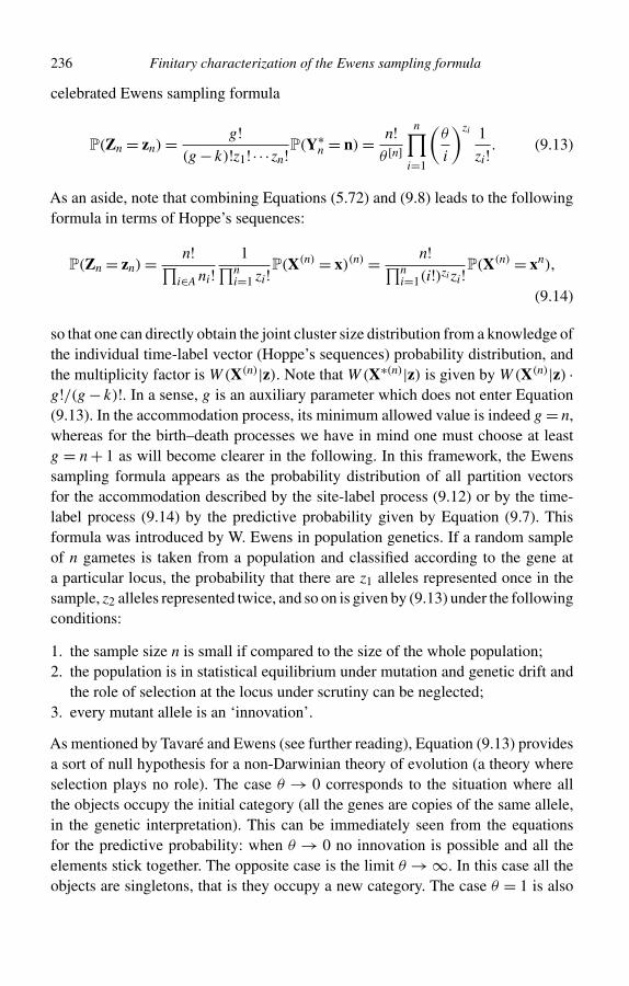
236 Finitary characterization of the Ewens sampling formula
celebrated Ewens sampling formula
P(Zn = zn) = g!(g − k)!z1! · · ·zn!P(Y∗
n = n) = n!θ [n]
n∏i=1
(θ
i
)zi 1
zi! . (9.13)
As an aside, note that combining Equations (5.72) and (9.8) leads to the followingformula in terms of Hoppe’s sequences:
P(Zn = zn) = n!∏i∈A ni!
1∏ni=1 zi!P(X(n) = x)(n) = n!∏n
i=1(i!)zi zi!P(X(n) = xn),
(9.14)
so that one can directly obtain the joint cluster size distribution from a knowledge ofthe individual time-label vector (Hoppe’s sequences) probability distribution, andthe multiplicity factor is W (X(n)|z). Note that W (X∗(n)|z) is given by W (X(n)|z) ·g!/(g − k)!. In a sense, g is an auxiliary parameter which does not enter Equation(9.13). In the accommodation process, its minimum allowed value is indeed g = n,whereas for the birth–death processes we have in mind one must choose at leastg = n + 1 as will become clearer in the following. In this framework, the Ewenssampling formula appears as the probability distribution of all partition vectorsfor the accommodation described by the site-label process (9.12) or by the time-label process (9.14) by the predictive probability given by Equation (9.7). Thisformula was introduced by W. Ewens in population genetics. If a random sampleof n gametes is taken from a population and classified according to the gene ata particular locus, the probability that there are z1 alleles represented once in thesample, z2 alleles represented twice, and so on is given by (9.13) under the followingconditions:
1. the sample size n is small if compared to the size of the whole population;2. the population is in statistical equilibrium under mutation and genetic drift and
the role of selection at the locus under scrutiny can be neglected;3. every mutant allele is an ‘innovation’.
As mentioned by Tavaré and Ewens (see further reading), Equation (9.13) providesa sort of null hypothesis for a non-Darwinian theory of evolution (a theory whereselection plays no role). The case θ → 0 corresponds to the situation where allthe objects occupy the initial category (all the genes are copies of the same allele,in the genetic interpretation). This can be immediately seen from the equationsfor the predictive probability: when θ → 0 no innovation is possible and all theelements stick together. The opposite case is the limit θ → ∞. In this case all theobjects are singletons, that is they occupy a new category. The case θ = 1 is also
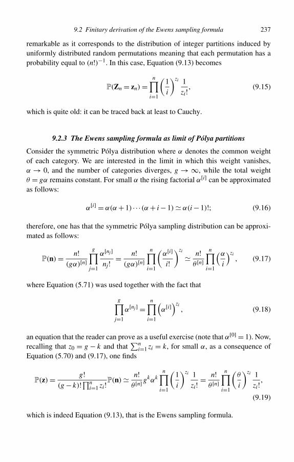
9.2 Finitary derivation of the Ewens sampling formula 237
remarkable as it corresponds to the distribution of integer partitions induced byuniformly distributed random permutations meaning that each permutation has aprobability equal to (n!)−1. In this case, Equation (9.13) becomes
P(Zn = zn) =n∏
i=1
(1
i
)zi 1
zi! , (9.15)
which is quite old: it can be traced back at least to Cauchy.
9.2.3 The Ewens sampling formula as limit of Pólya partitions
Consider the symmetric Pólya distribution where α denotes the common weightof each category. We are interested in the limit in which this weight vanishes,α → 0, and the number of categories diverges, g → ∞, while the total weightθ = gα remains constant. For small α the rising factorial α[i] can be approximatedas follows:
α[i] = α(α + 1) · · ·(α + i − 1) α(i − 1)!; (9.16)
therefore, one has that the symmetric Pólya sampling distribution can be approxi-mated as follows:
P(n) = n!(gα)[n]
g∏j=1
α[nj]
nj! = n!(gα)[n]
n∏i=1
(α[i]
i!)zi
n!θ [n]
n∏i=1
(α
i
)zi, (9.17)
where Equation (5.71) was used together with the fact that
g∏j=1
α[nj] =n∏
i=1
(α[i])zi
, (9.18)
an equation that the reader can prove as a useful exercise (note that α[0] = 1). Now,recalling that z0 = g − k and that
∑ni=1 zi = k, for small α, as a consequence of
Equation (5.70) and (9.17), one finds
P(z) = g!(g − k)!∏n
i=1 zi!P(n) n!θ [n] gkαk
n∏i=1
(1
i
)zi 1
zi! = n!θ [n]
n∏i=1
(θ
i
)zi 1
zi! ,
(9.19)
which is indeed Equation (9.13), that is the Ewens sampling formula.
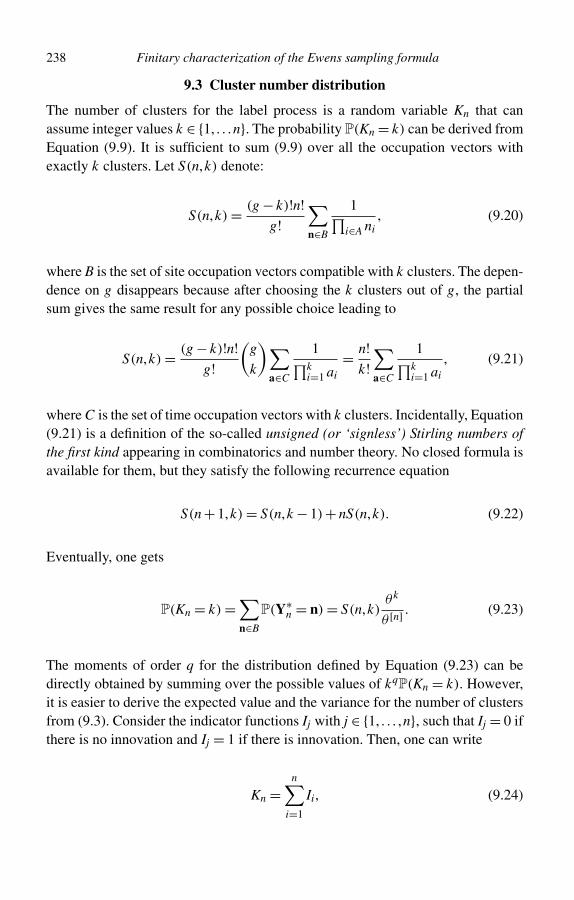
238 Finitary characterization of the Ewens sampling formula
9.3 Cluster number distribution
The number of clusters for the label process is a random variable Kn that canassume integer values k ∈ {1, . . .n}. The probability P(Kn = k) can be derived fromEquation (9.9). It is sufficient to sum (9.9) over all the occupation vectors withexactly k clusters. Let S(n,k) denote:
S(n,k) = (g − k)!n!g!
∑n∈B
1∏i∈A ni
, (9.20)
where B is the set of site occupation vectors compatible with k clusters. The depen-dence on g disappears because after choosing the k clusters out of g, the partialsum gives the same result for any possible choice leading to
S(n,k) = (g − k)!n!g!
(g
k
)∑a∈C
1∏ki=1 ai
= n!k!∑a∈C
1∏ki=1 ai
, (9.21)
where C is the set of time occupation vectors with k clusters. Incidentally, Equation(9.21) is a definition of the so-called unsigned (or ‘signless’) Stirling numbers ofthe first kind appearing in combinatorics and number theory. No closed formula isavailable for them, but they satisfy the following recurrence equation
S(n + 1,k) = S(n,k − 1)+ nS(n,k). (9.22)
Eventually, one gets
P(Kn = k) =∑n∈B
P(Y∗n = n) = S(n,k)
θ k
θ [n] . (9.23)
The moments of order q for the distribution defined by Equation (9.23) can bedirectly obtained by summing over the possible values of kqP(Kn = k). However,it is easier to derive the expected value and the variance for the number of clustersfrom (9.3). Consider the indicator functions Ij with j ∈ {1, . . . ,n}, such that Ij = 0 ifthere is no innovation and Ij = 1 if there is innovation. Then, one can write
Kn =n∑
i=1
Ii, (9.24)
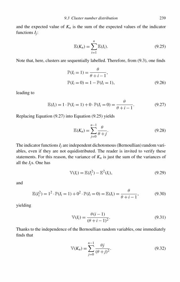
9.3 Cluster number distribution 239
and the expected value of Kn is the sum of the expected values of the indicatorfunctions Ij:
E(Kn) =n∑
i=1
E(Ii). (9.25)
Note that, here, clusters are sequentially labelled. Therefore, from (9.3), one finds
P(Ii = 1) = θ
θ + i − 1,
P(Ii = 0) = 1 −P(Ii = 1), (9.26)
leading to
E(Ii) = 1 ·P(Ii = 1)+ 0 ·P(Ii = 0) = θ
θ + i − 1. (9.27)
Replacing Equation (9.27) into Equation (9.25) yields
E(Kn) =n−1∑j=0
θ
θ + j. (9.28)
The indicator functions Ij are independent dichotomous (Bernoullian) random vari-ables, even if they are not equidistributed. The reader is invited to verify thesestatements. For this reason, the variance of Kn is just the sum of the variances ofall the Ijs. One has
V(Ii) = E(I2i )−E2(Ii), (9.29)
and
E(I2i ) = 12 ·P(Ii = 1)+ 02 ·P(Ii = 0) = E(Ii) = θ
θ + i − 1, (9.30)
yielding
V(Ii) = θ(i − 1)
(θ + i − 1)2. (9.31)
Thanks to the independence of the Bernoullian random variables, one immediatelyfinds that
V(Kn) =n−1∑j=0
θ j
(θ + j)2. (9.32)
240 Finitary characterization of the Ewens sampling formula
9.4 Ewens’ moments and site-label marginals
Returning to the site-label process, assume that n elements are classified into g > nsites. As in Section 5.3.8, one can introduce the indicator function IY ∗
j =i = I (i)Y ∗
j,
which is one if and only if site j exactly contains i elements. As an immediateconsequence of Equation (5.74), the number of clusters of size i is then given by
Zi =g∑
j=1
I (i)Y ∗
j, (9.33)
and
E(Zi) =g∑
j=1
P(Y ∗j = i) = gP(Y ∗
1 = i), (9.34)
due to the equidistribution of the g categories. Note that P(Y ∗1 = i) is the marginal
of (9.9) and can be obtained from the auxiliary urn model of the label process.In the Chinese restaurant example, the site marginal description is simply the
occupation number of a table fixed in advance. Indeed, after n accommodations,the occupation number of the table can be 1, . . . ,n, but also 0.
Consider the sequence X∗f = (X ∗
1 = 1, . . . ,X ∗i = 1,X ∗
i+1 �= 1, . . .X ∗n �= 1); its
probability is
P(X ∗1 = 1, . . . ,X ∗
i = 1,X ∗i+1 �= 1, . . . ,X ∗
n �= 1) = θ
g
(i − 1)!θ [n−i]
θ [n] . (9.35)
This equation can be justified as follows. Based on (9.7), one finds that
P(X ∗1 = 1,X ∗
2 = 1, . . . ,X ∗i = 1) = 1
g
1
θ + 1· · · (i − 1)
θ + i − 1= θ
g
(i − 1)!θ [i] , (9.36)
then, the next predictive step leads to
P(X ∗1 = 1, . . . ,X ∗
i = 1,X ∗i+1 �= 1)
= P(X ∗i+1 �= 1|X ∗
1 = 1, . . . ,X ∗i = 1)P(X ∗
1 = 1, . . . ,X ∗i = 1)
= (1 −P(X ∗i+1 = 1|X ∗
1 = 1, . . . ,X ∗i = 1))P(X ∗
1 = 1, . . . ,X ∗i = 1)
=(
1 − i
θ + i
)θ
g
(i − 1)!θ [i] = θ
θ + i
θ
g
(i − 1)!θ [i] , (9.37)
9.4 Ewens’ moments and site-label marginals 241
and the second next predictive step to
P(X ∗1 = 1, . . . ,X ∗
i = 1,X ∗i+1 �= 1,Xi+2 �= 1)
=(
1 − i
θ + i + 1
)θ
θ + i
θ
g
(i − 1)!θ [i] = θ + 1
θ + i + 1
θ
θ + i
θ
g
(i − 1)!θ [i] ; (9.38)
iterating this procedure leads to (9.35). Due to exchangeability, the probability ofany sequence with the same number of 1s as X∗
f is the same. This yields
P(Y ∗1 = i) = n!
i!(n − i)!P(X∗f ) = θ
gi
θ [n−i]/(n − i)!θ [n]/n! , (9.39)
and, as a consequence of Equation (9.34), one can derive the expected cluster sizes
E(Zi) = θ
i
θ [n−i]/(n − i)!θ [n]/n! . (9.40)
From Equations (9.34) and (9.40), one can compute
P(Y ∗i = 0) = g −E(Kn)
g, (9.41)
which is an increasing function of g; this is also the probability of finding an emptytable after a random selection among them.
Regarding the second moments of the cluster size, the derivation is similar. Forthe sake of simplicity, denote by R a sequence of n− i− j individual values differentfrom both 1 and 2 (again, the choice of the category/cluster labels is arbitrary). Usingthe method outlined above, one can prove that
P(X ∗1 = 1, . . . ,X ∗
i = 1,X ∗i+1 = 2, . . . ,X ∗
i+j = 2,R)
= θ2
g(g − 1)
(i − 1)!(j − 1)!θ [n−i−j]
θ [n] . (9.42)
As before, due to exchangeability, one finds
P(Y ∗1 = i,Y ∗
2 = j) = n!i!j!(n − i − j)!
θ2
g(g − 1)
(i − 1)!(j − 1)!θ [n−i−j]
θ [n]
= 1
g(g − 1)
θ2
ij
θ [n−i−j]/(n − i − j)!θ [n]/n! , (9.43)
242 Finitary characterization of the Ewens sampling formula
where, thanks to equidistribution, 1 and 2 can be replaced by any couple of labels.Now, consider the random variable Z2
i ; from Equations (5.74) and (9.33), it isgiven by
Z2i =
g∑l=1
I (i)Y ∗
l
g∑k=1
I (i)Y ∗
k=
g∑l=1
I (i)Y ∗
l+
g∑l=1
g∑k=l+1
I (i)Y ∗
lI (i)Y ∗
k
= Zi +g∑
l=1
g∑k=l+1
I (i)Y ∗
lI (i)Y ∗
k, (9.44)
as (I (i)Y ∗
l)2 = I (i)
Y ∗l
. Using the result of Exercise 5.3, one finds
E
(Z2
i
)= E(Zi)+
g∑l=1
g∑k=l+1
P(Y ∗
l = i,Y ∗k = i
)= E(Zi)+ g (g − 1)P
(Y ∗
1 = i,Y ∗2 = i
), (9.45)
for integer i ≤ n/2; otherwise, the second term vanishes. Replacing Equation (9.43)into Equation (9.45) with i = j leads to
E
(Z2
i
)=E(Zi)+
(θ
i
)2 n!(n − 2i)!
θ [n−2i]
θ [n], if i integer ≤ n
2E(Zi) otherwise.
(9.46)
In a similar way, one can derive that
E(ZiZj
)= θ2
ij
n!(n − i − j)!
θ [n−i−j]
θ [n], i + j ≤ n. (9.47)
In the limit n � θ , one has
θ [n]
n! ≈ nθ−1
(θ − 1)! , (9.48)
then the above-mentioned moments of Zi can be approximated as follows:
E(Zi) ≈ θ
i
(1 − i
n
)θ−1
, (9.49)
E
(Z2
i
)≈ E(Zi)+
(θ
i
)2(1 − 2i
n
)θ−1
, (9.50)
9.5 Alternative derivation of the expected number of clusters 243
and
E(ZiZj
)≈ θ2
ij
(1 − i + j
n
)θ−1
, (9.51)
and so on. In the continuous limit n →∞, if the fractional size x = i/n is introduced,Equation (9.49) converges to the so-called frequency spectrum introduced by Ewensin his 1972 paper and defined by
f (x) = θ
x(1 − x)θ−1 , (9.52)
with x ∈ (0,1]. The interval open to the left means nothing else but that the minimumfractional size is 1/n. The meaning of
f (x)dx = θ
x(1 − x)θ−1 dx (9.53)
is the average fraction of clusters whose fractional size is between x and x + dx,whereas θ (1 − x)θ−1 dx is the average mass fraction allocated to clusters whosefractional size is between x and x + dx.
9.5 Alternative derivation of the expected number of clusters
The distribution of cluster sizes can be directly derived from Equation (9.3), withoutan extensive analysis of the label process.Alittle thought reveals that, given a clustersize frequency Zn = zn, if one samples an element, all elements being on a par, andone observes the size of the cluster to which this element belongs, the probabilitythat the first observed cluster Y1 contains i elements is just
P(Y1 = i|Zn = zn) = izi
n; (9.54)
therefore, as a consequence of the total probability theorem, one finds
P(Y1 = i) =∑zn
P(Y1 = i|Zn = zn)P(Zn = zn) = iE(Zi)
n. (9.55)
This leads to
E(Zi) = n
iP(Y1 = i); (9.56)
in other words, the probabilistic study of the first cluster is sufficient to get theexpected distribution of the cluster size. Consider the fundamental sequence Xf =
244 Finitary characterization of the Ewens sampling formula
(X1 = 1, . . . ,Xi = 1,Xi+1 > 1, . . . ,Xn > 1). Considering that the marginal eventXj > 1 is the complement of Xj = 1, the very same method used to derive Equation(9.35) leads to
P(X1 = 1, . . . ,Xi = 1,Xi+1 > 1, . . . ,Xn > 1) = θ(i − 1)!θ [n−i]
θ [n] ; (9.57)
then, one finds that
P(Y1 = i) =(
n − 1
i − 1
)P(Xf ), (9.58)
due to the fact that X1 = 1 and the other i − 1 variables corresponding to the firstcluster can always be chosen among n − 1 variables. Eventually, this leads to
P(Y1 = i) = θ
n
θ [n−i]/(n − i)!θ [n]/n! , (9.59)
in agreement with Equation (9.39). Combining Equation (9.56) with Equation(9.59), Equation (9.40) is recovered. Given that (θ + 1)[n−1] = θ [n]/θ , Equation(9.59) can be re-written as follows
P(Y1 = i) =(
n − 1
i − 1
)1[i−1]θ [n−i]
(θ + 1)[n−1] , (9.60)
which is nothing other than the Polya(i −1,n−1;1,θ). In the continuum limit, theprobability density function of the fractional size of the first cluster (i/n) is thendistributed according to Beta(1,θ).
9.6 Sampling and accommodation
Before introducing a Markovian probabilistic model leading to equilibrium clus-ter distributions given by the equations discussed in the previous sections of thischapter, it is useful to further discuss the meaning of the two processes discussedso far.
9.6.1 Sampling from a random distribution
Consider a system of n elements, and imagine that the only available information isthat they are grouped in some number of clusters, say Kn, and there are Z1,n clusterswith one element, Z2,n clusters with two elements, and so on, so that
∑ni=1 Zi,n = Kn.
9.6 Sampling and accommodation 245
The only certain piece of information is that∑n
i=1 iZi,n = n. Further assume thatP(Zn = zn) is given by Equation (9.13). Now, Zn is no more completely unknown,it is still indeterminate, but its uncertainty is ruled by the sampling formula dueto Ewens. While in statistics this uncertainty is based on Bayesian roots, in thecase under scrutiny, it has a realistic root, as the system will be allowed to changein time, and P(Zn = zn) is proportional to the time fraction in which the clusterstatistical distribution is given by Zn = zn. Sampling from this random distributionmeans taking a snapshot of the moving population, and then observing all theelements in a sequence. The sequence X1, . . . ,Xn describes the elements sampledwithout replacement. If the sampling hypothesis is that all sequences conditionedto the present partition value zn are equiprobable, the probability of any sequence isgiven by Equation (9.4) and the predictive sampling probability is then (9.3).1 Thismeans that the first element observed belongs to the first cluster with probability 1,the second element either belongs to the first cluster with probability 1/(1 + θ) orit belongs to a new cluster (the second one) with probability θ/(1 + θ), and so on.After observing m agents, the (m+1)th belongs to a not yet observed (new) clusterwith probability θ/(m + θ), whereas the total probability of an already observedcluster is m/(m + θ).
Another type of sampling from the partition value z corresponding to k clustersis the so-called species sampling. It amounts to classifying the size of the k clustersin the order in which they appear if all the elements are equiprobably drawn withoutreplacement. The distribution of the first pick was derived in the previous section.The cluster sizes are represented by the time-label frequency vector a. A littlethought leads to the following equation
P(a|z) = a1
n
a2
n − a1· · · ak−1
ak−1 + ak
ak
ak
n∏i=1
zi!; (9.61)
indeed, if all the clusters had different sizes and∏n
i=1 zi! = 1, these terms woulddescribe the probability of drawing an element of the jth cluster from a population inwhich the elements belonging to the already observed clusters have been removed;if there were more than a single cluster of size i, the first time one selects a clusterof this size, the total probability mass is proportional to izi, the second time itis proportional to i(zi − 1), and so on. Equation (9.61) is called the size biasedpermutation of z, as all the clusters belonging to z appear in (9.61), but their orderof appearance is biased due to their size, meaning that different permutations havedifferent probabilities. Given that P(a) = P(a|z)P(z), if P(a|z) is given by (9.61)
1 This duality between predictive inferences and sampling from a random distribution is well known in the realmof Bayesian statistics, and it is based on de Finetti’s representation theorem for exchangeable sequences (seeSection 4.3).
246 Finitary characterization of the Ewens sampling formula
and P(z) is the Ewens sampling formula (9.13), it should be clear why Equation(9.6) was called the size-biased permutation of the Ewens sampling formula byDonnelly.
9.6.2 The accommodation process
Now change perspective and consider a population of n agents that can chooseamong a large number of possible strategies/choices. The names of these strategiesare not interesting, and one wishes to study the way in which agents partition intogroups, it being understood that two units belong to the same cluster if and onlyif Xi = Xj. The operational frame is the one of the Chinese restaurant described inSection 9.1.1. Agents choose sequentially, and each agent’s choice is conditionedby the previous accommodation. Even if the possible strategies/choices are infinite,no more than n can be exploited by a finite population of n elements; therefore,we describe the possible choices by considering a system of g > n labels or sites.Considering the conceptual difference between a cluster and a site, it is sufficientto say that when a cluster dies, it disappears forever, whereas a site can be occupiedagain. The only meaning of these labels is that of distinguishing between differentclusters, and, ceteris paribus, the labels are set equiprobable. Then, the first agentchooses the jth site with uniform probability 1/g. The second has two possibilities:if his/her choice is the same as the first (‘herding’), he/she accommodates in thesame site; if it is different (‘innovation’), he/she accommodates in a site labelled,say, by i, with i �= j, with probability 1/(g − 1) uniform on the remaining emptysites. It is assumed that the choice is probabilistic, and influenced by the previousresults with the weight of ‘innovation’ set equal to θ .
Hoppe’s predictive probability (9.3) is a description of a sampling sequence interms of time labels (the time of appearance of the clusters in sampling). On thecontrary, the accommodation probability (9.7) is a description of a physical process,and it uses site labels that can be regarded as usual permanent categories.
The essential difference between the two types of label is given by the factor1/(g − Km) for the probability of innovations. In the case of time labels the nameof a new cluster is already determined, whereas for sites it must be chosen. In thiscase one can pass from time labels to site labels by fixing the Kn cluster labelsindependently on anything. If g labels are available, each of the g(g − 1) · · ·(g −Kn +1) = g!/(g −Kn)! site descriptions is equally likely. These considerations leadto Equation (9.8).
As the clustering structure of the accommodation process is the same as (9.3),one can conclude that the size of the first cluster (also known as the size-biasedpick) is ruled by Equation (9.59), the statistical cluster distribution has probabilitygiven by Equation (9.13) and the average number of clusters of size i is given by
9.7 Markov chains for cluster and site dynamics 247
(9.40). In this framework, all these distributions have an objective meaning: if onebuilds an ensemble of independent accommodation processes with the same initialconditions, the frequency of any event in the ensemble is roughly proportionalto the corresponding probability. Note that Zn is ‘random’, or, better, ruled by(9.13), because it is generated by a random mechanism (the accommodation process,agents’ choices).
9.7 Markov chains for cluster and site dynamics
9.7.1 Ehrenfest–Brillouin with infinite categories
At the beginning of this chapter, we were looking for random variables suitablefor building an irreducible and aperiodic Markov chain in the case of an infinitenumber of categories. This is why the site-label process was introduced. In theChinese restaurant example, suppose that the n customers, once accommodated,are free to move from one table to another. If they join an already occupied table,their behaviour can be called ‘herding’; if they move to an empty table, they arecalled ‘pioneers’. Note that, in the usual accommodation process, whose probabilityis proportional to αi +ni, if an element moves to a non-empty category, it cannot beidentified either as a follower of the herd or as a follower of the initial distribution.On the contrary, when the number of categories becomes infinite and their weightvanishes, the two behaviours cannot give rise to the same choice. Indeed, the domainof the initial distribution is infinite and this means that the probability of choosingany finite number of fixed tables is zero. Consequently, with probability 1, a followerof the theoretical distribution is compelled to choose an empty table and, therefore,he/she is a pioneer, that is the founder of a new cluster.
The model outlined above has several possible interpretations in economics. Ifoccupied tables represent firms, the elements may be agents who move from onefirm to another, or create new firms. Elements may also be agents who choose differ-ent strategies (clusters). Another possible interpretation is that elements representfirms, and clusters economic sectors. It is possible to interpret elements as firmsand clusters as regional sites as well, and so on. Considering the interpretation interms of workers in firms, if the number of sites g > n there is always room foropening a new firm. Among the g sites, there will always be k ≤ n < g living firmswhile the g − k empty ones are ready to be occupied by pioneers.
In order to represent these features by means of a homogeneous Markov chain, themain route is introducing the ‘label-site process’, simplifying a method suggestedby Kelly. This method is very similar to the Ehrenfest–Brillouin model, and isthe subject of the next section. A second way is to abandon once and for all thelabels of the categories and directly to study partition vectors. The Markov chain
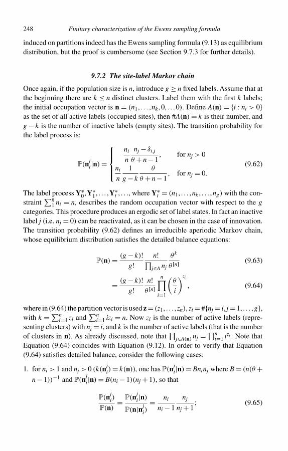
248 Finitary characterization of the Ewens sampling formula
induced on partitions indeed has the Ewens sampling formula (9.13) as equilibriumdistribution, but the proof is cumbersome (see Section 9.7.3 for further details).
9.7.2 The site-label Markov chain
Once again, if the population size is n, introduce g ≥ n fixed labels. Assume that atthe beginning there are k ≤ n distinct clusters. Label them with the first k labels;the initial occupation vector is n = (n1, . . . ,nk ,0, . . .0). Define A(n) = {i : ni > 0}as the set of all active labels (occupied sites), then #A(n) = k is their number, andg − k is the number of inactive labels (empty sites). The transition probability forthe label process is:
P(nji|n) =
ni
n
nj − δi,j
θ + n − 1, for nj > 0
ni
n
1
g − k
θ
θ + n − 1, for nj = 0.
(9.62)
The label process Y∗0,Y∗
1, . . . ,Y∗t , . . ., where Y∗
t = (n1, . . . ,nk , . . . ,ng) with the con-straint
∑g1 ni = n, describes the random occupation vector with respect to the g
categories. This procedure produces an ergodic set of label states. In fact an inactivelabel j (i.e. nj = 0) can be reactivated, as it can be chosen in the case of innovation.The transition probability (9.62) defines an irreducible aperiodic Markov chain,whose equilibrium distribution satisfies the detailed balance equations:
P(n) = (g − k)!g!
n!∏j∈A nj
θk
θ [n] (9.63)
= (g − k)!g!
n!θ [n]
n∏i=1
(θ
i
)zi
, (9.64)
where in (9.64) the partition vector is used z = (z1, . . . ,zn), zi = #{nj = i, j = 1, . . . ,g},with k =∑n
i=1 zi and∑n
i=1 izi = n. Now zi is the number of active labels (repre-senting clusters) with nj = i, and k is the number of active labels (that is the numberof clusters in n). As already discussed, note that
∏j∈A(n) nj =∏n
i=1 izi . Note thatEquation (9.64) coincides with Equation (9.12). In order to verify that Equation(9.64) satisfies detailed balance, consider the following cases:
1. for ni > 1 and nj > 0 (k(nji) = k(n)), one has P(nj
i|n) = Bninj where B = (n(θ +n − 1))−1 and P(nj
i|n) = B(ni − 1)(nj + 1), so that
P(nji)
P(n)= P(nj
i|n)
P(n|nji)
= ni
ni − 1
nj
nj + 1; (9.65)
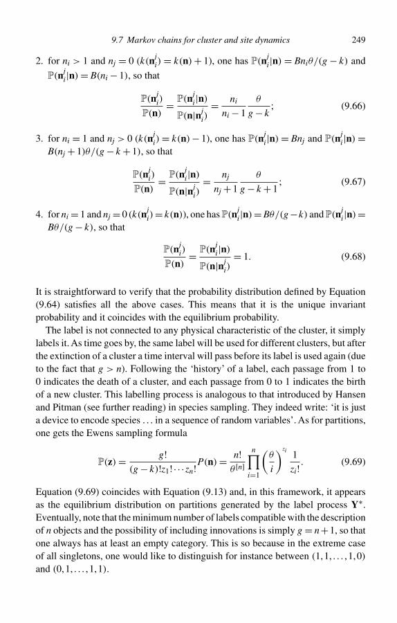
9.7 Markov chains for cluster and site dynamics 249
2. for ni > 1 and nj = 0 (k(nji) = k(n) + 1), one has P(nj
i|n) = Bniθ/(g − k) and
P(nji|n) = B(ni − 1), so that
P(nji)
P(n)= P(nj
i|n)
P(n|nji)
= ni
ni − 1
θ
g − k; (9.66)
3. for ni = 1 and nj > 0 (k(nji) = k(n)− 1), one has P(nj
i|n) = Bnj and P(nji|n) =
B(nj + 1)θ/(g − k + 1), so that
P(nji)
P(n)= P(nj
i|n)
P(n|nji)
= nj
nj + 1
θ
g − k + 1; (9.67)
4. for ni = 1 and nj = 0 (k(nji)= k(n)), one has P(nj
i|n)= Bθ/(g−k) and P(nji|n)=
Bθ/(g − k), so that
P(nji)
P(n)= P(nj
i|n)
P(n|nji)
= 1. (9.68)
It is straightforward to verify that the probability distribution defined by Equation(9.64) satisfies all the above cases. This means that it is the unique invariantprobability and it coincides with the equilibrium probability.
The label is not connected to any physical characteristic of the cluster, it simplylabels it. As time goes by, the same label will be used for different clusters, but afterthe extinction of a cluster a time interval will pass before its label is used again (dueto the fact that g > n). Following the ‘history’ of a label, each passage from 1 to0 indicates the death of a cluster, and each passage from 0 to 1 indicates the birthof a new cluster. This labelling process is analogous to that introduced by Hansenand Pitman (see further reading) in species sampling. They indeed write: ‘it is justa device to encode species . . . in a sequence of random variables’. As for partitions,one gets the Ewens sampling formula
P(z) = g!(g − k)!z1! · · ·zn!P(n) = n!
θ [n]n∏
i=1
(θ
i
)zi 1
zi! . (9.69)
Equation (9.69) coincides with Equation (9.13) and, in this framework, it appearsas the equilibrium distribution on partitions generated by the label process Y∗.Eventually, note that the minimum number of labels compatible with the descriptionof n objects and the possibility of including innovations is simply g = n+1, so thatone always has at least an empty category. This is so because in the extreme caseof all singletons, one would like to distinguish for instance between (1,1, . . . ,1,0)
and (0,1, . . . ,1,1).
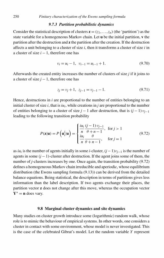
250 Finitary characterization of the Ewens sampling formula
9.7.3 Partition probabilistic dynamics
Consider the statistical description of clusters z = (z1, . . . ,zn) (the ‘partition’) as thestate variable for a homogeneous Markov chain. Let u be the initial partition, v thepartition after the destruction and z the partition after the creation. If the destructionaffects a unit belonging to a cluster of size i, then it transforms a cluster of size i ina cluster of size i − 1, therefore one has
vi = ui − 1, vi−1 = ui−1 + 1. (9.70)
Afterwards the created entity increases the number of clusters of size j if it joins toa cluster of size j − 1, therefore one has
zj = vj + 1, zj−1 = vj−1 − 1. (9.71)
Hence, destructions in i are proportional to the number of entities belonging to aninitial cluster of size i, that is iui, while creations in j are proportional to the numberof entities belonging to a cluster of size j − 1 after destruction, that is (j − 1)vj−1
leading to the following transition probability
P(z|u) = P(
uji|u)
=
iui
n
(j − 1)vj−1
θ + n − 1, for j > 1
iui
n
θ
θ + n − 1, for j = 1
(9.72)
as iui is the number of agents initially in some i-cluster, (j−1)vj−1 is the number ofagents in some (j −1)-cluster after destruction. If the agent joins some of them, thenumber of j-clusters increases by one. Once again, the transition probability (9.72)defines a homogeneous Markov chain irreducible and aperiodic, whose equilibriumdistribution (the Ewens sampling formula (9.13)) can be derived from the detailedbalance equations. Being statistical, the description in terms of partitions gives lessinformation than the label description. If two agents exchange their places, thepartition vector z does not change after this move, whereas the occupation vectorY∗ = n does vary.
9.8 Marginal cluster dynamics and site dynamics
Many studies on cluster growth introduce some (logarithmic) random walk, whoserole is to mimic the behaviour of empirical systems. In other words, one considers acluster in contact with some environment, whose model is never investigated. Thisis the case of the celebrated Gibrat’s model. Let the random variable Y represent
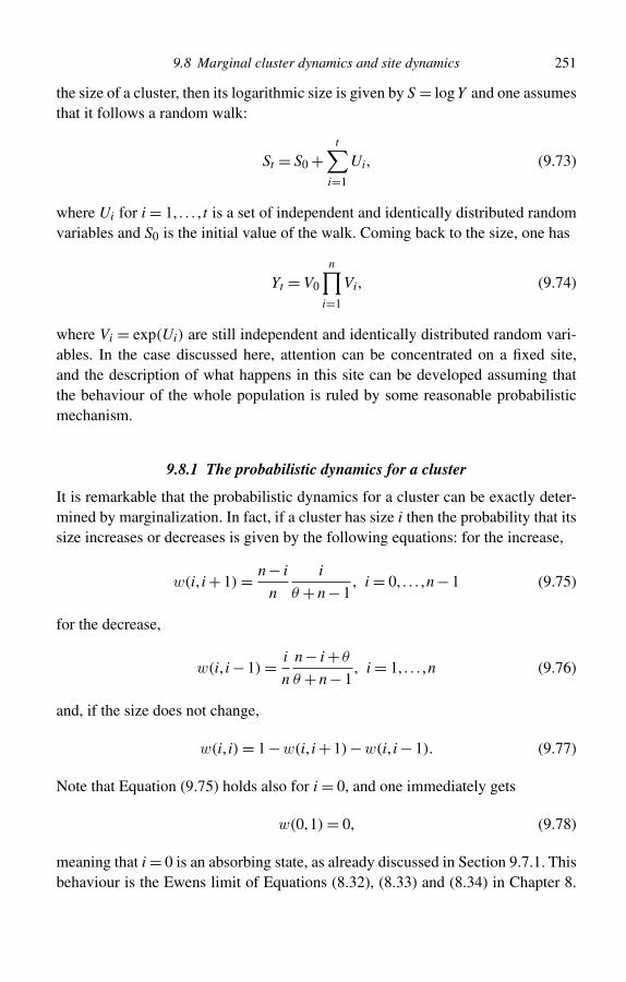
9.8 Marginal cluster dynamics and site dynamics 251
the size of a cluster, then its logarithmic size is given by S = logY and one assumesthat it follows a random walk:
St = S0 +t∑
i=1
Ui, (9.73)
where Ui for i = 1, . . . , t is a set of independent and identically distributed randomvariables and S0 is the initial value of the walk. Coming back to the size, one has
Yt = V0
n∏i=1
Vi, (9.74)
where Vi = exp(Ui) are still independent and identically distributed random vari-ables. In the case discussed here, attention can be concentrated on a fixed site,and the description of what happens in this site can be developed assuming thatthe behaviour of the whole population is ruled by some reasonable probabilisticmechanism.
9.8.1 The probabilistic dynamics for a cluster
It is remarkable that the probabilistic dynamics for a cluster can be exactly deter-mined by marginalization. In fact, if a cluster has size i then the probability that itssize increases or decreases is given by the following equations: for the increase,
w(i, i + 1) = n − i
n
i
θ + n − 1, i = 0, . . . ,n − 1 (9.75)
for the decrease,
w(i, i − 1) = i
n
n − i + θ
θ + n − 1, i = 1, . . . ,n (9.76)
and, if the size does not change,
w(i, i) = 1 −w(i, i + 1)−w(i, i − 1). (9.77)
Note that Equation (9.75) holds also for i = 0, and one immediately gets
w(0,1) = 0, (9.78)
meaning that i = 0 is an absorbing state, as already discussed in Section 9.7.1. Thisbehaviour is the Ewens limit of Equations (8.32), (8.33) and (8.34) in Chapter 8.
252 Finitary characterization of the Ewens sampling formula
Hence, given that E( Y |Y = i) = w(i, i + 1) − w(i, i − 1), with Y = Yt+1 − Yt ,one finds
E( Y |Y = i) = − i
n
θ
θ + n − 1= −ri, (9.79)
where r is the rate of approach of the conditional expected value to equilibriumfor unary moves (see Section 8.2.2). Note that (9.79) is a particular case of (8.43)when the equilibrium mean is zero. In other words, each particular existing clusteris driven towards extinction with the rate defined by Equation (9.79). The matrixw(i, j) drives the evolution of the represented cluster. All the states except for i = 0are transient, and the state i = 0 is absorbing. In order to study the time behaviourof a cluster, one can use w(s)(i, j), that is the transition probability from i to j after ssteps. Then w(s)(i,0) is the probability that a cluster of size i will die after s steps.If the random variable Di denotes the number of time steps from size i to death,one can write
P(Di ≤ s) = w(s)(i,0). (9.80)
Therefore, the difference w(s)(i,0) − w(s−1)(i,0) gives the probability of dyingexactly at the sth step for a cluster of size i. In symbols, one can write
P(Di = s) = P(Di ≤ s)−P(Di ≤ s − 1) = w(s)(i,0)−w(s−1)(i,0), (9.81)
as the event {Di ≤ s} is the union of two disjoint events: {Di ≤ s} = {Di = s}∪{Di ≤s − 1}. The variable τi given by
τi = E(Di) =∞∑
s=1
s(w(s)(i,0)−w(s−1)(i,0)) (9.82)
is the expected duration time of a cluster of size i. Note that from (9.75), (9.76)and (9.77), one has w(s)(i,0)−w(s−1)(i,0) = w(s−1)(i,1)/n, as dying at the sth stepis the same as reaching size 1 at the (s − 1)th step and then dying with transitionprobability w(1,0) = 1/n from (9.75). Hence, one finds
τi =∞∑
s=1
sw(s−1)(i,1)
n, (9.83)
where w(0)(i,1) = δi,1. The expected duration time of a new cluster (of size 1,τ1) is the expected life of a newborn cluster. It can be exactly computed fromEquation (9.83), but an alternative derivation is possible. In fact considering that
9.8 Marginal cluster dynamics and site dynamics 253
r = θ/(θ +n−1) is the innovation rate, that is the expected number of new clustersat each step, and using E(Kn), the stationary expected number of clusters, theaverage life of a new cluster is just
τ1 = E(Kn)
r, (9.84)
where E(Kn) is given by Equation (9.28). A recurrence relation exists for τi, so thatit can be found avoiding the sum in Equation (9.83). In fact if a cluster has size i (andits expected duration time is τi), at the following step there are three possibilities,and three possible expected duration times, all increased by the duration of the step(= 1). Therefore
τi = w(i, i + 1){τi+1 + 1}+w(i, i){τi + 1}+w(i, i + 1){τi−1 + 1}, (9.85)
that is
τi = 1 +w(i, i + 1)τi+1 +w(i, i)τi +w(i, i − 1)τi−1, (9.86)
and replacing Equations (9.75), (9.76) and (9.77), reordering and defining τi =τi − τi−1, i ≥ 2 with τ0 = 0 leads to
τi = τi−1n − i + 1 + θ
n − i + 1− n(n − 1 + θ)
(i − 1)(n − i + 1), τ1 = E(Kn)
u. (9.87)
9.8.2 The probabilistic dynamics for a site
If a site is considered instead of a cluster, there is the possibility of rebirth. When asite is empty, an agent occupying another site can decide to move to the empty site. Ifthe site contains i agents, the probabilistic dynamics is given by the same equationsas before, namely Equations (9.75), (9.76) and (9.77). All the other occupied sitesare merged in a single one (the thermostat), whose weight is n − i, plus θ , thatis the weight of the empty sites. Note that the cluster dynamics described in theprevious section does not depend on the number of clusters Kn and thus it can beexactly discussed. Considering the site dynamics, if the site is empty, i = 0, onecan introduce the rebirth term and its complement
w(0,1) = 1
g − Kn
θ
θ + n − 1,
w(0,0) = 1 −w(0,1); (9.88)
in this way, the state Y ∗ = 0 is no longer absorbing. Note that w(0,1) depends on Kn
and g, so that this term contains an exogenous random variable. This is not essential
254 Finitary characterization of the Ewens sampling formula
for the equilibrium distribution of the cluster size. Starting from a cluster whosesize is i, the history of the cluster (that ends when the size reaches i = 0) must bedistinguished from that of the site, that sooner or later reactivates. Then, the birth–death chain defined by Equations (9.75), (9.76), (9.77) and (9.88) is irreducibleand aperiodic, and its stationary and equilibrium distribution satisfies the detailedbalance condition
P(Y ∗ = i + 1)i + 1
n
n − i − 1 + θ +α
θ + n − 1= P(Y ∗ = i)
n − i
n
i −α
θ + n − 1, (9.89)
for i = 1, . . . ,n − 1, and
P(Y ∗ = 1)w(1,0) = P(Y ∗ = 0)w(0,1), (9.90)
thus leading to
P(Y ∗ = i + 1)
P(Y ∗ = i)= n − i
i + 1
i
θ + n − i − 1= E(Zi+1)
E(Zi), (9.91)
where E(Zi) is just the expected cluster size given by (9.40) in the Ewens population,whereas P(Y ∗ = i) is the marginal distribution of the Ewens population (Equation(9.39)). The term P(Y ∗ = 0) depends on g and Kn. If, in Equation (9.88), Kn isreplaced by E(Kn), at best, the chain mimics what happens at the fixed site if itshistory is drawn from the exact joint dynamics of the whole population. But whatis essential from the cluster point of view is that w(0,1) is positive. If for instanceg � n, each fixed site is going to be empty for a long period of time. If one chooses asite at random, all sites being equiprobable, the site will be empty with probability(g − E(Kn))/g and E(Kn)/g is the probability of finding a living cluster. Then,randomly choosing a cluster, all clusters being equiprobable, and observing, itssize is described by
P(Y ∗ = i|i > 0) = E(Zi)
E(Kn), i = 1, . . . ,n, (9.92)
it being understood that any observation concerns living clusters (non-empty sites).
9.8.3 A simple example on workers and firms
Consider a population of n workers following an aggregation dynamics driven byEquations (9.2), and therefore, at equilibrium, described by the Ewens samplingformula parameters n and θ . Given that En(Zi,n) = (n/i) · Polya(i − 1,n − 1;1,θ),in order to simplify calculations suppose that θ = 1. Then one gets Polya(i −1,n−
9.8 Marginal cluster dynamics and site dynamics 255
1;1,1) = 1/n, and E(Zi,n) = 1/i. Now Polya(i − 1,n − 1;1,1) is the probabilitydistribution of the first pick, whose meaning is: if one samples a worker at random,that is all workers are on a par, and one asks the size of the firm to which theworker belongs, then the answer will be uniformly distributed on {1, . . . ,n}. Onecan assume that the worker spends his time in all possible firm sizes uniformly.For instance, there is the same probability of finding him alone (as a singleton) asof finding him employed in a monopolistic firm of size n. The expected numberof firms for size 1,2, . . . ,n is 1,1/2,1/3, . . . ,1/n, that is one expects a singleton inevery snapshot of the population, a couple every two snapshots, ..:, a monopolisticsize n every n snapshots. Hence the expected mass of workers in firms of size iis iE(Zi,n) = 1, which is uniform, and explains why the first pick (sampling a sizebiased by the number of workers) is uniform. On the contrary, if one chooses a firm,equiprobably drawn among the existing ones, and observes its size, one finds thatthis random variable is distributed as E(Zi,n)/E(Kn) = i−1/E(Kn), with E(Kn) =∑n
i=1 i−1, and the odds of a singleton against the monopoly are n : 1. If one sam-ples the site-labels, the denominator is g, and one finds that 1 − E(Kn)/g is theprobability of finding an empty site, while i−1/g is the absolute probability for thesize i. Following the link given by Equation (9.55), i−1/E(Kn) is the equilibriumprobability for the marginal chain of a firm as long as it is alive. It can be inter-preted as the visiting time relative frequency for the size i during the life of thecluster.
Suppose that n = 10: the expected number of firms is E(Kn) = 2.93. Assume thatthe first pick gives a1 = 4, whose probability is P(a1 = 4) = 1/10. What can wesay about a2? It is not difficult to show that in general P(a2|a1) = Polya(a2 −1,n−a1 −1;1,θ), that is: the second pick has the same distribution as the first, within therestricted domain n − a1; and this holds true for all k clusters. Hence the sequencea1 = 4,a2 = 6 has probability 1/10 · 1/6 = 1/60. If one considers the permutationa1 = 6,a2 = 4, its probability is 1/10 · 1/4 = 1/40, which is greater than 1/60,due to the intuitive fact that the order of appearance is positively correlated withthe size of the cluster. Both permutations are the only possibilities belonging to(z4 = z6 = 1), whose probability is given by Equation (9.13), and is just equal to(1/4) · (1/6) = 1/24 = 1/40 + 1/60.
Considering the continuum limit n → ∞, the probability of a size-biasedsequence x1,x2, . . . ,with xi = ai/n, is obtained considering that residual fractionsx1,x2/(1 − x1), . . . ,xi+1/(1 − x1 − . . .− xi) are all distributed according to the dis-tribution Beta(1,θ). This way of assigning probability to the sequence is calledthe Residual Allocation Model (RAM), as all residuals are independent; moreover,being also identically distributed as Beta(1,θ), the distribution is called GEM byTavaré and Ewens (see further reading), after Griffiths, Engen and McCloskey.
256 Finitary characterization of the Ewens sampling formula
9.9 The two-parameter Ewens process
9.9.1 Definition of the process
Hansen and Pitman generalized the Ewens sampling formula described in thischapter. Their generalization can be discussed in a rather elementary way with thetools developed above. Equation (9.2) is modified as follows
P(Xn+1 = j|X1 = x1, . . . ,Xn = xn) =
nj −α
θ + n, for j ≤ k
θ +αk
θ + n, for j = k + 1
(9.93)
with 0 ≤ α < 1 and θ + α > 0. In Equation (9.93), if the parameter α is positive,the probability of choosing a new cluster increases proportionally to the number ofexisting clusters Kn = k, whereas for each existing cluster, the probability of beingoccupied decreases with respect to the Ewens case. This process can be modelledby means of a two-parameter Hoppe’s urn, as described by Zabell in his 1992 paperPredicting the Unpredictable (see further reading):
Imagine an urn containing both colored and black balls, from which balls are both drawnand then replaced. Each time a colored ball is drawn, it is put back into the urn, togetherwith a new ball with the same color having a unit weight, each time a black ball is selected,it is put back into the urn, together with two new balls, one black and having weight α, andone of a new color, having weight 1 −α. Initially the urn contains a single black ball (themutator).
In other words, if an already observed colour is drawn, the updating mechanism isPólya (the weight of the colour increases by one), while a new colour receives aninitial weight equal to 1−α. If α = 0 the model reduces to a conventional Hoppe’surn. The case α > 0 implies an increasing weight α for the mutator every time itis drawn (a new colour appears). However, the model can be extended to α < 0,in which case the weight of the mutator decreases every time it is drawn. If θ =k|α|, after k colours have appeared no new colour can be drawn. Hence, samplingcoincides with a k-dimensional Pólya sampling with uniform initial weights equalto |α|. The only difference is that in the k-dimensional Pólya sampling the namesof the categories are known in advance, and the initial weights are not forced to beuniform.
The method described in Section 9.5 applied to the predictive probability (9.93)immediately leads to the distribution of the first cluster picked:
P(Y1 = i) = θ(1 −α)[i−1]
n(i − 1)!(θ +α)[n−i]/(n − i)!
θ [n]/n! , (9.94)
9.9 The two-parameter Ewens process 257
that can also be written similarly to Equations (9.58) and (9.59) as
P(Y1 = i) =(
n − 1
i − 1
)(1 −α)[i−1](θ +α)[n−i]
(1 + θ)[n−1] . (9.95)
Equation (9.95) is a generalization of Equation 9.60 and is simply the dichotomousPólya distribution of initial weights 1 −α and θ +α for i − 1 hits over n − 1 trials.In the continuum limit, the density of the fractional size for the first cluster (i/n)is then distributed according to Beta(1 − α,θ + α). This result is not surprising atall. Indeed, the two-parameter Pólya urn described above coincides with the usualdichotomous Pólya urn with initial weights 1 − α and θ + α and unitary prize,when the first drawn colour is taken into account. If one finds i − 1 times the firstdrawn colour in the successive n − 1 draws, then the final size of the first colourdrawn from the urn is i. As before, one can find E(Zi) multiplying (9.95) by n/i.Regarding Markovian dynamics, referring to the methods developed in Section 9.8,the first moment of the equilibrium cluster size distribution is obtained from theequilibrium marginal distribution for a site. The only difference is that the first twoEquations (9.75) and (9.76) are replaced by
w(i, i + 1) = n − i
n
i −α
θ + n − 1, (9.96)
and by
w(i, i − 1) = i
n
n − i + θ +α
θ + n − 1, (9.97)
respectively.
9.9.2 Expected number of clusters
A typical example of the usefulness of the finite approach to the two-parameterEwens distribution is the exact calculation of the equilibrium average number ofclusters as a function of α,θ ,n. Let us consider the balance between death and birth.If the system is described by {Zi,n}, considering unary changes, a cluster dies if andonly if the extracted unit belongs to a singleton, hence the probability of a death isz1,n/n. A new cluster is born if the extracted unit is a pioneer, and, given that thepioneering probability depends on the actual number of present clusters, we mustdistinguish the case in which the accommodating unit comes from a singleton,where the actual number of clusters is Kn−1 = Kn − 1, from the alternative one,
258 Finitary characterization of the Ewens sampling formula
where the actual number of clusters is Kn−1 = Kn. HenceP(death|zn) = z1,n
n,
P(birth|zn) = z1,n
n
θ + (kn − 1)α
n − 1 + θ+(
1 − z1,n
n
) θ + knα
n − 1 + θ.
(9.98)
Now
z1,n
n
θ + (kn − 1)α
n − 1 + θ+(
1 − z1,n
n
) θ + knα
n − 1 + θ
= 1
n(n − 1 + θ)
(z1,n(θ + (kn − 1)α − θ − knα)+ n(θ + knα)
)= 1
n(n − 1 + θ)
(−z1,nα + n(θ + knα))
. (9.99)
The unconditional death (and birth) probabilities are:P(death) =∑zn
P(death|zn)P(zn) = E(Z1,n)
n,
P(birth) = 1
n(n − 1 + θ)
(−E(Z1,n)α + n(θ +E(Kn)α))
,(9.100)
and the equilibrium balance implies
E(Z1,n) = −E(Z1,n)α
n − 1 + θ+ θ +E(Kn)α
n − 1 + θ, (9.101)
that gives
E(Kn) = E(Z1,n)n − 1 + θ +α
nα− θ
α. (9.102)
Introducing in (9.102) the value
E(Z1,n) = θn(θ +α)[n−1]
θ [n] = n(θ +α)[n−1]
(θ + 1)[n−1] , (9.103)
from (9.95), we find
E(Kn) = θ
α
((θ +α)[n]
θ [n] − 1
). (9.104)
9.10 Summary 259
The fact that E(Kn) in (9.104) is exactly equal to∑n
i=1 E(Zi,n) from (9.95) iseasy to check numerically. Further it is easy to show that for small α,
(θ +α)[n]
θ [n] = (θ +α)
θ
(θ +α + 1)
θ + 1. . .
(θ +α + n − 1)
θ + n − 1
=(
1 + α
θ
)(1 + α
θ + 1
). . .
(1 + α
θ + n − 1
)= 1 +
n∑i=1
α
θ + i − 1+ o(α). (9.105)
Hence
E(Kn) = θ
α
n∑i=1
α
θ + i − 1+ o(α) =
n∑i=1
θ
θ + i − 1+ o(α), (9.106)
where
n∑i=1
θ
θ + i − 1= E0,θ (Kn) (9.107)
is the well-known expected number of clusters in the one-parameter Ewens case.In the opposite limit α → 1, we have
E(Kn) → θ
((θ + 1)[n]
θ [n] − 1
)= θ
(θ + n
θ− 1
)= n, (9.108)
as the population is composed of all singletons with probability one.For large n, (9.104) can be approximated by
E(Kn) θ
α
(�(θ)
�(θ +α)nα − 1
) �(θ + 1)
�(θ +α)
nα
α. (9.109)
9.10 Summary
In this chapter the problem of allocating n elements into d � n categories/clusterswas discussed. This problem allows us to take into account innovations, namelywhen an element joins an empty category: in practice, this can be interpreted as anovelty not seen before.
It turns out that the joint distribution of cluster sizes is described by the so-called Ewens sampling formula. Two derivations of this formula were presented.The first makes use of the so-called site label process, in which, every time a new
260 Finitary characterization of the Ewens sampling formula
category/cluster appears, a label is assigned randomly drawn from a predefinedset. The second directly uses the order of appearance in order to time-label a newcluster.
It is possible to modify the Ehrenfest–Brillouin Markov chain discussed inChapter 7 in order to take innovations into account. When the resulting modelis properly interpreted it turns out that a cluster sooner or later disappears. It is theninteresting to study the distribution of lifetimes for a cluster of given size as well asits expected lifetime. On the contrary, a site can resuscitate leading to an aperiodicand irreducible Markov chain, with the Ewens sampling formula being the jointprobability distribution for the size of the sites. Suitable birth–death chains describethe marginal probabilistic dynamics evolution for a cluster and for a site.
Finally, a generalization of the Ewens distribution to two parameters is possible.Both parameters rule the probability of innovations which, in this case, also dependson the total number of clusters.
Further reading
Ewens introduced his sampling formula in a 1972 paper
W.J. Ewens, The Sampling Theory of Selectively Neutral Alleles, Theoretical PopulationBiology, 3, 87–112 (1972).
There is a tutorial paper written byTavaré and Ewens that summarizes many relevantresults including some of the equations derived in this chapter
S. Tavaré and W.J. Ewens, Multivariate Ewens Distribution in N.L. Johnson, S. Kotz andN. Balakrishnan (eds), Discrete Multivariate Distributions, Wiley, New York (1997).
Donnelly’s paper introducing the size-biased permutation of the Ewens samplingformula appeared in 1986
P. Donnelly, Partition Structures, Pólya Urns, the Ewens Sampling Formula and the Agesof Alleles, Theoretical Population Biology, 30, 271–288 (1986).
One year later, Hoppe published his own paper on the sampling theory of neutralalleles
F.M. Hoppe, The Sampling Theory of Neutral Alleles and an Urn Model in PopulationGenetics, Journal of Mathematical Biology, 25, 123–159 (1987).
where his urn model was discussed.All the above papers concern the one-parameter Ewens sampling formula and are
devoted to its applications in biology. The two-parameter generalization discussedin Section 9.9 was introduced by Hansen and Pitman
B. Hansen and J. Pitman, Prediction Rules for Exchangeable Sequences Related to SpeciesSampling, Statistics and Probability Letters, 46, 251–256 (2000).
9.10 Summary 261
but Zabell anticipated it in his 1992 work on predictive inferences
S. Zabell, Predicting the Unpredictable, Synthese, 90, 205–232 (1992).
Aoki applied these methods to the formation of clusters in economics
M. Aoki, New Approaches to Macroeconomic Modeling: Evolutionary Stochastics Dynam-ics, Multiple Equilibria and Externalities as Field Effects, Cambridge University Press,Cambridge, UK (1996).
M. Aoki, Cluster Size Distribution of Economic Agents of Many Types in a Market, Journalof Mathematical Analysis and Applications, 249, 32–52 (2000).
M. Aoki, Modeling Aggregate Behavior and Fluctuations in Economics, CambridgeUniversity Press, Cambridge, UK (2002).
The finitary version discussed in this chapter was studied in a series of papersco-authored by Garibaldi
U. Garibaldi, D. Costantini and P. Viarengo, A Finite Characterization of Ewens SamplingFormula, Advances in Complex Systems, 7, 265–284 (2003).
U. Garibaldi, D. Costantini and P. Viarengo, A Finitary Characterization of Ewens SamplingFormula in T. Lux, S. Reitz and E. Samanidou (eds), Nonlinear Dynamics and Heteroge-neous Interacting Agents, Lecture Notes in Economics and Mathematical Systems, 550,Springer, Berlin (2005).
U. Garibaldi, D. Costantini and P. Viarengo, The Two-parameter Ewens Distribution: aFinitary Approach, Journal of Economic Interaction and Coordination, 2, 147–161 (2007).
Readers interested in Gibrat’s model may consult his book
R. Gibrat, Les Inégalités Économiques, Librairie du Recueil Sirey, Paris (1931).
A recent account of his ideas is also available
M. Armatte, Robert Gibrat and the Law of Proportional Effect in W.J. Samuels (ed.), Euro-pean Economists of the Early 20th Century vol. I, Edward Elgar Publishing, Northampton,UK (1998).
Random walks and multiplicative processes are dealt with in many textbooksalready quoted in previous chapters.
10
The Zipf–Simon–Yule process
This chapter is devoted to a modification of the Chinese restaurant example inwhich the probability of choosing a new table is a fixed parameter u and no longerdepends on the number of previous customers. This leads to a non-exchangeableaccommodation process. The final sections of this chapter deal with the continuouslimit of finite birth-and-death chains.
After reading this chapter, you should be able to:
• understand why Zipf’s process is not exchangeable;• understand the meaning of Simon’s regression;• derive the Yule distribution in various ways;• write a Monte Carlo program for cluster dynamics leading to cluster-size
distributions with power-law tails;• discuss the continuous limit of discrete birth-and-death Markov chains.
10.1 The Ewens sampling formula and firm sizes
To understand the rationale for this chapter, it is useful to compare the Ewens sam-pling formula with empirical data on firm sizes. In Section 9.7.1, various economicinterpretations of the model under scrutiny were given. Indeed, one can considerthe elements as workers and the clusters as firms. For the dynamics discussed inSection 9.8.2, and for n � θ , one finds that E(Zi) is given by Equation (9.49). Onecan further note that, by definition,
n∑i=1
E(Zi) = E(Kn), (10.1)
and that, in the limit of large n, due to Equation (9.28), one finds
E(Kn) =n−1∑i=0
θ
θ + i≈ θ ln
n + θ
θ+ γ , (10.2)
262
10.2 Hoppe’s vs. Zipf’s urn 263
where γ is Euler’s constant. Note that E(Zi) is the expected number of firms of size iwhen the size of the population is n. The meaning of E(Kn) in the firm size problemis the equilibrium expected number of firms, which increases logarithmically withtotal number of individual agents n. For a comparison with empirical data, E(Zi)
and E(Kn) are the theoretical quantities to be compared with empirical values.In particular, E(Zi)/E(Kn) is the expected fraction of firms of size i. From themarginal point of view, this ratio gives the time fraction spent by a firm in thestate corresponding to size i. A remarkable case of Equation (9.49) is found whenθ = 1. If θ = 1, then E(Zi) = 1/i. In other words, the expected firm size follows apower law. This looks promising, but it is deceiving. In the case of USA firms, forinstance, the rough number of firms is k = 5.5 · 106 and the number of workers isabout n = 105 ·106. In the Ewens model, given n, the only parameter to be fixed isθ , whose best estimate can be found from the empirical value of k. Inverting (10.2),one gets θ = 1.24 · 106, and in that region the normalized Equation (9.49) cannotbe distinguished from
E(Zi) ≈ θ
iexp(−iθ/n). (10.3)
This can be represented by the log-series distribution
L(i) = − 1
log(1 − y)
yi
i, y = 1,2, . . . (10.4)
where the parameter is y = exp(−θ/n). In this limit, the normalizing constant givenin Equation (10.2) becomes
E(Kn) = θ lnn
θ. (10.5)
It follows that the size distribution is approximately proportional to θ/i for smallsizes, but has an exponential tail for large sizes. This is sufficient to exclude a Ewens-like dynamics producing equilibrium probabilities whose tail follows a power law.Therefore, it is necessary to define a new cluster dynamics leading to a power-lawdistribution of cluster sizes.
10.2 Hoppe’s vs. Zipf’s urn
Consider the label process for Hoppe’s urn. Using the indicator functions Inj=0
which is 1 when Y ∗j = nj = 0 and 0 for Y ∗
j = nj > 0 and its complement
264 The Zipf–Simon–Yule process
Inj>0 = 1 − Inj=0, Equation (9.7) can be written in a single line
P(X ∗n+1 = j|nj,n) = n
n + θ
nj
nInj>0 + θ
n + θ
1
g − KnInj=0, (10.6)
where all the parameters and variables have the same meaning as in Chapter 9.Once more, note that at the beginning of this process, the probability of selectingone of the g categories/sites is given by 1/g and this is automatically included inEquations (9.7) and (10.6). In the right-hand side of Equation (10.6), the first termdescribes herding as it gives the probability of joining an already existing clusterof size j, whereas the second term describes innovation because it is the probabilityof founding a new cluster in an empty site as a pioneer. In Chapter 9, it was shownthat the label process is exchangeable. For example, the probability of the sequenceX ∗
1 = i,X ∗2 = j,X ∗
3 = i (with i �= j) is
P(X ∗1 = i,X ∗
2 = j,X ∗3 = i) = 1
g(g − 1)
θ2
θ(θ + 1)(θ + 2), (10.7)
and it coincides with the probability of any permutation of the values, that is withthe probability of the sequences X ∗
1 = i,X ∗2 = i,X ∗
3 = j and X ∗1 = j,X ∗
2 = i,X ∗3 = i.
The label process for Zipf’s urn can be defined in a similar way. One can write forn > 0
P(X ∗n+1 = j|nj,n) = (1 − u)
nj
nInj>0 + u
1
g − KnInj=0, (10.8)
where 0 < u < 1 is the probability of innovation which is now independent of nand its complement 1 − u is the probability of herding, whereas for n = 0, one has
P(X ∗1 = j) = 1
g. (10.9)
A direct application of Equation (10.8) on the sequences X ∗1 = i,X ∗
2 = j,X ∗3 =
i and X ∗1 = i,X ∗
2 = i,X ∗3 = j immediately shows that this process is no longer
exchangeable. Indeed, one has
P(X ∗1 = i,X ∗
2 = j,X ∗3 = i) = 1
2
u(1 − u)
g(g − 1), (10.10)
whereas
P(X ∗1 = i,X ∗
2 = i,X ∗3 = j) = u(1 − u)
g(g − 1). (10.11)
10.3 Expected cluster size dynamics and the Yule distribution 265
Given that the process of individual sequences is not exchangeable, the methodsintroduced in Section 5.3.8 and used in Chapters 7, 8 and 9 cannot be applied inorder to derive the distribution of cluster sizes. In 1955, Simon, aware or not ofthe problem, studied the expected cluster dynamics as a way to circumvent thisproblem and obtain quantitative results. His method is described in the next sectionusing the terminology developed in the previous chapters.
10.3 Expected cluster size dynamics and the Yule distribution
Simon refers to the sequential construction of a text adding a new word at each step.This is equivalent to considering a new customer entering the Chinese restaurantand choosing an existing table (a word already written in the text) or a new table(a new word not yet used in the text). Here, instead of using site labels as in theprevious section, it is useful to refer to time labels. Equation (10.8) modifies to
P(Xn+1 = j|nj,n) = (1 − u)nj
nIj≤Kn + uIj=Kn+1. (10.12)
Simon assumes that you are writing a text using the following rules. You havealready written n words. If zi,n is the number of words appearing i times in the text,the probability of using one of these words at the next step is proportional to izi,n;the probability of using a new word not yet present in the text is constant and equalto u with 0 < u < 1. Note that the first word in the text is new with probability 1.Moreover, if u = 0, no innovation is possible and P(Zn,n = 1) = 1, in other words,there is only a cluster containing n repetitions of the same word. On the contrary,if u = 1, every word included in the text is a new word not yet used; therefore, inthis case, the text is made up of n distinct words meaning that there are n clusterseach containing 1 element, so that one has P(Z1,n = n) = 1. If Yn+1 = i denotesthe event that the (n + 1)th word is among the words that occurred i times, andYn+1 = 0 means that the (n+1)th word is a new one, Equation (10.12) leads to thefollowing probabilities conditioned on the partition vector Zn = zn:
P(Yn+1 = i|Zn = zn) = (1 − u)izi,n
n,
P(Yn+1 = 0|Zn = zn) = u, n > 0
P(Y1 = 0) = 1.
(10.13)
The evolution of the partition vector is as follows. If Yn+1 = i, it implies that acluster of size i is destroyed and a cluster of size i + 1 is created meaning thatzi,n+1 = zi,n −1 and zi+1,n+1 = zi+1,n +1. If Yn+1 = 0, it means that a cluster of size1 is created, that is z1,n+1 = z1,n + 1. Consider now the random variable difference
266 The Zipf–Simon–Yule process
Zi,n+1 −Zi,n; it can assume two values, one has Zi,n+1 −Zi,n = 1 if a cluster of size(i − 1) is destroyed and a cluster of size i is created, and Zi,n+1 − Zi,n = −1 if acluster of size i is destroyed and a cluster of size i +1 is created. As a consequenceof Equation (10.13), one has for i = 2, . . . ,n
P(Zi,n+1 − Zi,n = 1|Zn = zn) = (1 − u)(i − 1)zi−1,n
n, (10.14)
and
P(Zi,n+1 − Zi,n = −1|Zn = zn) = (1 − u)izi,n
n. (10.15)
Therefore, considering that E(Zi,n|Zn = zn) = zi,n for any i, one finds that
E(Zi,n+1|Zn = zn)− zi,n = (1 − u)
((i − 1)zi−1,n
n− izi,n
n
), (10.16)
an equation valid for i = 2, . . . ,n. For i = 1, as a consequence of Equation (10.13),one finds that
E(Z1,n+1|Zn = zn)− z1,n = u − (1 − u)z1,n
n. (10.17)
Defining the unconditional expected value of Zi+1,n
zi+1,n = E(Zi+1,n) =∑zn−1
E(Zi+1,n|Zn = zn)P(Zn = zn), (10.18)
one can derive the following equations by taking the expectations of (10.16) and(10.17):
zi,n+1 − zi,n = (1 − u)
((i − 1)zi−1,n
n− izi,n
n
), (10.19)
and
z1,n+1 − z1,n = u − (1 − u)z1,n
n. (10.20)
In principle, the recurrence Equations (10.19) and (10.20) can be directly solved.However, Simon suggests looking for solutions such that zi,n ∝ n corresponding toa steady growth of the clusters, that is, the fraction of clusters of size i tends to aconstant value as n grows. With Simon’s Ansatz, one has that
zi,n+1
zi,n= n + 1
n, (10.21)
10.3 Expected cluster size dynamics and the Yule distribution 267
equivalent to
zi,n+1 − zi,n = zi,n
n, (10.22)
for i = 1, . . . ,n. Replacing Equation (10.22) for i = 1 into Equation (10.20) gives
z∗1,n = nu
2 − u= ρ
1 +ρnu, (10.23)
where ρ > 1 is a parameter defined as
ρ = 1
1 − u. (10.24)
If Equation (10.22) is replaced into Equation (10.19), the recurrence equationsimplifies to
z∗i,n = (1 − u)(i − 1)
1 + (1 − u)iz∗
i−1,n = i − 1
ρ + iz∗
i−1,n. (10.25)
The iteration of (10.25) leads to a closed-form solution for z∗i,n:
z∗i,n = i − 1
ρ + i
i − 2
ρ + i − 1· · · 1
ρ + 2z∗
1,n = �(i)�(ρ + 2)
�(ρ + i + 1)z∗
1,n
= (ρ + 1)�(i)�(ρ + 1)
�(ρ + i + 1)z∗
1,n = ρB(i,ρ + 1)nu, (10.26)
where Equation (10.23) and the definition of Euler’s beta function (4.101) wereused. Direct replacement shows that Equation (10.26) is a solution of Equation(10.19). Note that the ratio zi,n/n on the left-hand side of Equation (10.22) is not afrequency. The expected number of clusters (of words in the text) is given by
E(Kn) =n∑
i=1
E(Zi,n) =n∑
i=1
z∗i,n = nu
n∑i=1
ρB(i,ρ + 1), (10.27)
and, summing up to infinity, it is possible to prove that
∞∑i=1
ρB(i,ρ + 1) = 1. (10.28)
Therefore, from Equation (10.13) one has that E(Kn) = 1 + (n − 1)u ≈ ν for largen, meaning that there is a constant flow of new words. In other words, Simon’s
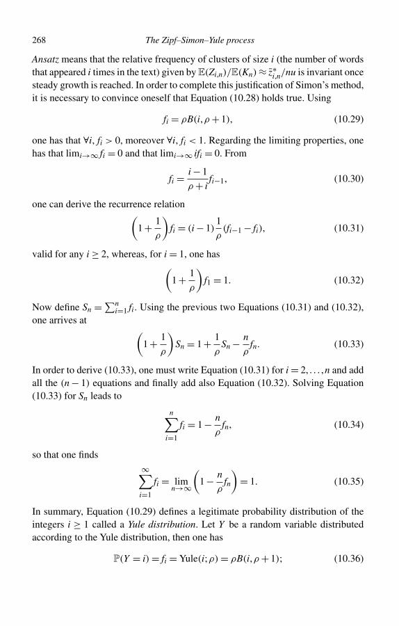
268 The Zipf–Simon–Yule process
Ansatz means that the relative frequency of clusters of size i (the number of wordsthat appeared i times in the text) given by E(Zi,n)/E(Kn) ≈ z∗
i,n/nu is invariant oncesteady growth is reached. In order to complete this justification of Simon’s method,it is necessary to convince oneself that Equation (10.28) holds true. Using
fi = ρB(i,ρ + 1), (10.29)
one has that ∀i, fi > 0, moreover ∀i, fi < 1. Regarding the limiting properties, onehas that limi→∞ fi = 0 and that limi→∞ ifi = 0. From
fi = i − 1
ρ + ifi−1, (10.30)
one can derive the recurrence relation(1 + 1
ρ
)fi = (i − 1)
1
ρ(fi−1 − fi), (10.31)
valid for any i ≥ 2, whereas, for i = 1, one has(1 + 1
ρ
)f1 = 1. (10.32)
Now define Sn =∑ni=1 fi. Using the previous two Equations (10.31) and (10.32),
one arrives at (1 + 1
ρ
)Sn = 1 + 1
ρSn − n
ρfn. (10.33)
In order to derive (10.33), one must write Equation (10.31) for i = 2, . . . ,n and addall the (n − 1) equations and finally add also Equation (10.32). Solving Equation(10.33) for Sn leads to
n∑i=1
fi = 1 − n
ρfn, (10.34)
so that one finds∞∑
i=1
fi = limn→∞
(1 − n
ρfn
)= 1. (10.35)
In summary, Equation (10.29) defines a legitimate probability distribution of theintegers i ≥ 1 called a Yule distribution. Let Y be a random variable distributedaccording to the Yule distribution, then one has
P(Y = i) = fi = Yule(i;ρ) = ρB(i,ρ + 1); (10.36)
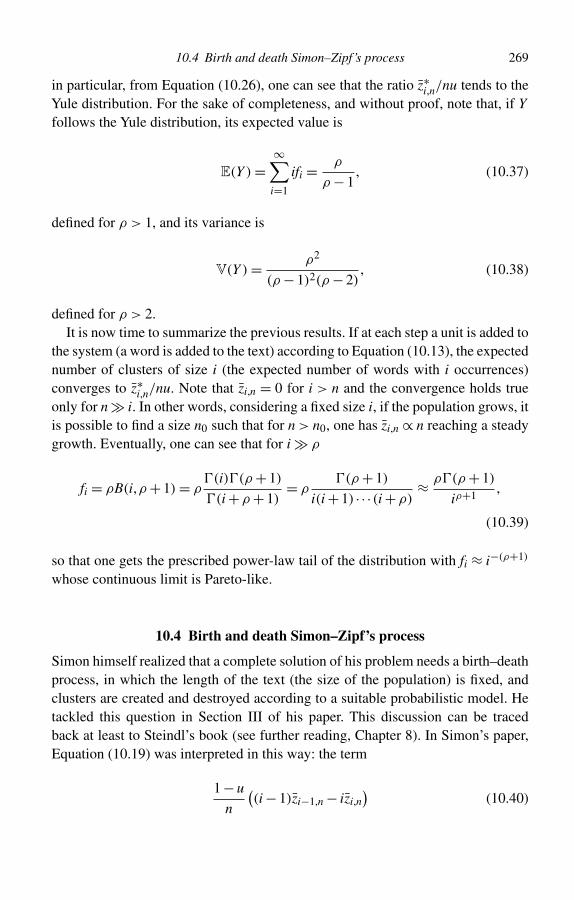
10.4 Birth and death Simon–Zipf’s process 269
in particular, from Equation (10.26), one can see that the ratio z∗i,n/nu tends to the
Yule distribution. For the sake of completeness, and without proof, note that, if Yfollows the Yule distribution, its expected value is
E(Y ) =∞∑
i=1
ifi = ρ
ρ − 1, (10.37)
defined for ρ > 1, and its variance is
V(Y ) = ρ2
(ρ − 1)2(ρ − 2), (10.38)
defined for ρ > 2.It is now time to summarize the previous results. If at each step a unit is added to
the system (a word is added to the text) according to Equation (10.13), the expectednumber of clusters of size i (the expected number of words with i occurrences)converges to z∗
i,n/nu. Note that zi,n = 0 for i > n and the convergence holds trueonly for n � i. In other words, considering a fixed size i, if the population grows, itis possible to find a size n0 such that for n > n0, one has zi,n ∝ n reaching a steadygrowth. Eventually, one can see that for i � ρ
fi = ρB(i,ρ + 1) = ρ�(i)�(ρ + 1)
�(i +ρ + 1)= ρ
�(ρ + 1)
i(i + 1) · · ·(i +ρ)≈ ρ�(ρ + 1)
iρ+1,
(10.39)
so that one gets the prescribed power-law tail of the distribution with fi ≈ i−(ρ+1)
whose continuous limit is Pareto-like.
10.4 Birth and death Simon–Zipf’s process
Simon himself realized that a complete solution of his problem needs a birth–deathprocess, in which the length of the text (the size of the population) is fixed, andclusters are created and destroyed according to a suitable probabilistic model. Hetackled this question in Section III of his paper. This discussion can be tracedback at least to Steindl’s book (see further reading, Chapter 8). In Simon’s paper,Equation (10.19) was interpreted in this way: the term
1 − u
n
((i − 1)zi−1,n − izi,n
)(10.40)
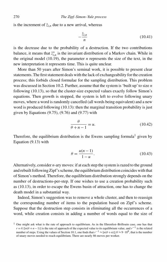
270 The Zipf–Simon–Yule process
is the increment of zi,n due to a new arrival, whereas
− zi,n
n(10.41)
is the decrease due to the probability of a destruction. If the two contributionsbalance, it means that z∗
i,n is the invariant distribution of a Markov chain. While inthe original model (10.19), the parameter n represents the size of the text, in thenew interpretation it represents time. This is quite unclear.
More than 50 years after Simon’s seminal work, it is possible to present clearstatements. The first statement deals with the lack of exchangeability for the creationprocess; this forbids closed formulae for the sampling distribution. This problemwas discussed in Section 10.2. Further, assume that the system is ‘built up’ to size nfollowing (10.13), so that the cluster-size expected values exactly follow Simon’sequations. Then growth is stopped, the system is left to evolve following unarymoves, where a word is randomly cancelled (all words being equivalent) and a newword is produced following (10.13): then the marginal transition probability is justgiven by Equations (9.75), (9.76) and (9.77) with
θ
θ + n − 1= u. (10.42)
Therefore, the equilibrium distribution is the Ewens sampling formula1 given byEquation (9.13) with
θ = u(n − 1)
1 − u. (10.43)
Alternatively, consider n-ary moves: if at each step the system is razed to the groundand rebuilt following Zipf’s scheme, the equilibrium distribution coincides with thatof Simon’s method. Therefore, the equilibrium distribution strongly depends on thenumber of destructions-per-step. If one wishes to use a creation probability suchas (10.13), in order to escape the Ewens basin of attraction, one has to change thedeath model in a substantial way.
Indeed, Simon’s suggestion was to remove a whole cluster, and then to reassignthe corresponding number of items to the population based on Zipf’s scheme.Suppose that the destruction step consists in eliminating all the occurrences of aword, while creation consists in adding a number of words equal to the size of
1 One might ask what is the rate of approach to equilibrium. As in the Ehrenfest–Brillouin case, one has thatr = θ/[n(θ +n−1)] is the rate of approach of the expected value to its equilibrium value, and r−1 is the relatednumber of steps. Using the values of Section 10.1, one finds that r−1 ≈ [n(θ +n)]/θ ≈ 9 ·109, that is the numberof unary moves needed to reach equilibrium. There are nearly 86 moves per worker.

10.5 Marginal description of the Simon–Zipf process 271
the destroyed cluster. First, one eliminates a cluster, all clusters being equivalent,and then one puts back the corresponding number of items into the populationfollowing Equation (10.13). At each step, the size of the population first diminishesby a random size m equal to the size of the destroyed cluster, and then returnsto its natural size n via m accommodations. Using the interpretation in terms offirms, at each step a firm dies, and all its workers either join existing firms orfound new ones with individual probability 1−u or u, respectively. Newborn firmsaccommodate in some empty site, and they are labelled by their site. The Markovchain of the site process is ergodic, but an analytic solution is cumbersome becausethe transition matrix is very complex, due to the lack of exchangeability for thecreation process. In Section II of his paper, Simon suggests that this approachis reasonable. Consider Equation (10.16) and compare it with (10.17). If all zi,n
are equal to their equilibrium expected value zi,n the increment of zi,n is given by(10.22). On the contrary, if zi−1,n = zi−1,n but zi,n = zi,n + εi,n, then, its expectedincrement E(zi,n+1 − zi,n) differs from the expected increment by a restoring term
−(1 − u)iεi,n
n. (10.44)
In words, on average, a fluctuation away from the expected value is smoothed bynew arrivals.
10.5 Marginal description of the Simon–Zipf process
If a cluster of size i is considered, belonging to a population whose dynamics isdescribed by the mechanism described in the previous section, one can see thatthe time evolution cannot be a simple function of i, n − i and u. In fact, the deathmechanism deeply differs from the Ewens case; it amounts to ‘killing’ a wholecluster, with equal probability for all the k active clusters (with 1 ≤ k ≤ n). Twocases are possible: the first is to assume that a destruction occurs at each step; inthe second case, one sets the probability of removing each existing cluster equal to1/n, so that the probability of removals is k/n ≤ 1, with the proviso that if no killingoccurs the system is left in the initial state. The second version can be interpretedsupposing that each cluster is represented by its elder worker. If at each step a unitis chosen, killing occurs when the elder worker is chosen. With this assumption theprobability of being killed, that is moving from size i to size 0, is
w(i,0) = 1
n. (10.45)
If another cluster dies, the cluster of size i can increase up to the (random) sizeof the destroyed cluster. When n � 1, as the probability of joining the cluster
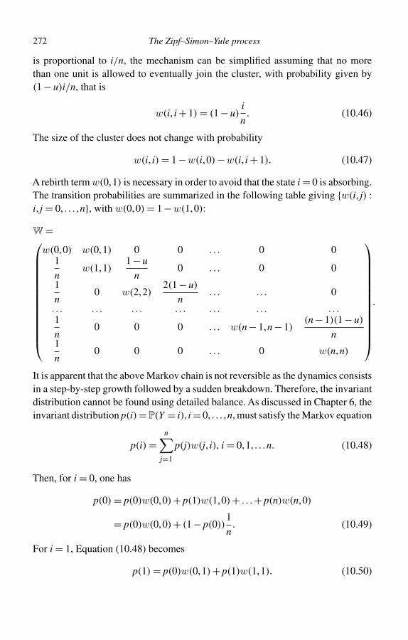
272 The Zipf–Simon–Yule process
is proportional to i/n, the mechanism can be simplified assuming that no morethan one unit is allowed to eventually join the cluster, with probability given by(1 − u)i/n, that is
w(i, i + 1) = (1 − u)i
n. (10.46)
The size of the cluster does not change with probability
w(i, i) = 1 −w(i,0)−w(i, i + 1). (10.47)
A rebirth term w(0,1) is necessary in order to avoid that the state i = 0 is absorbing.The transition probabilities are summarized in the following table giving {w(i, j) :i, j = 0, . . . ,n}, with w(0,0) = 1 −w(1,0):
W =
w(0,0) w(0,1) 0 0 . . . 0 01
nw(1,1)
1 − u
n0 . . . 0 0
1
n0 w(2,2)
2(1 − u)
n. . . . . . 0
. . . . . . . . . . . . . . . . . . . . .1
n0 0 0 . . . w(n − 1,n − 1)
(n − 1)(1 − u)
n1
n0 0 0 . . . 0 w(n,n)
.
It is apparent that the above Markov chain is not reversible as the dynamics consistsin a step-by-step growth followed by a sudden breakdown. Therefore, the invariantdistribution cannot be found using detailed balance. As discussed in Chapter 6, theinvariant distribution p(i)= P(Y = i), i = 0, . . . ,n, must satisfy the Markov equation
p(i) =n∑
j=1
p(j)w(j, i), i = 0,1, . . .n. (10.48)
Then, for i = 0, one has
p(0) = p(0)w(0,0)+ p(1)w(1,0)+ . . .+ p(n)w(n,0)
= p(0)w(0,0)+ (1 − p(0))1
n. (10.49)
For i = 1, Equation (10.48) becomes
p(1) = p(0)w(0,1)+ p(1)w(1,1). (10.50)
10.5 Marginal description of the Simon–Zipf process 273
For 1 ≤ i < n the generic term is
p(i) = p(i − 1)w(i − 1, i)+ p(i)w(i, i); (10.51)
it can be re-written as
p(i)(1 −w(i, i)) = p(i − 1)w(i − 1, i). (10.52)
Using Equations (10.45), (10.46) and (10.47) leads to
p(i)
(1
n+ (1 − u)
i
n
)= p(i − 1)
(1 − u)(i − 1)
n. (10.53)
This equation coincides with (10.25). The explicit form of p(i) is
p(i) = θi−1
ϕ + θi. . .
θ1
ϕ + θ2
θ0
ϕ + θ1
ϕ
ϕ + θ0, (10.54)
where θi = w(i, i + 1) and ϕ = 1/n. The equation
p(0) = ϕ
ϕ + θ0(10.55)
can be interpreted as the probability (the fraction of time) that the label is idle.Conditioning on the time fraction in which the cluster is alive, that is introducing
πi = P(Y = i|i > 0) = p(i)
1 − p(0)= p(i)
ϕ + θ0
θ0, (10.56)
one obtains
πi = θi−1
ϕ + θi. . .
θ1
ϕ + θ2
ϕ
ϕ + θ1, (10.57)
a result that does not depend on the rebirth term θ0. Note that
θi−1
ϕ + θi=
i − 1
nρ
1
n+ i
nρ
= i − 1
ρ + i, (10.58)
274 The Zipf–Simon–Yule process
so that
π1 = 1
1 + (1 − u)= ρ
ρ + 1,
π2 = ρ
ρ + 1
1
ρ + 2,
π3 = ρ
ρ + 1
1
ρ + 2
2
ρ + 3, . . . (10.59)
Therefore, it turns out that
πi = ρ�(i)�(ρ + 1)
�(ρ + i + 1)= ρB(i,ρ + 1) i = 1, . . . ,n − 1; (10.60)
this is exactly the value of the Yule distribution (10.29). The term πn is different,as θn = 0; therefore, one finds
πn = θn−1
ϕ + θnπn−1 = n − 1
ρπn−1 �= n − 1
ρ + nπn−1. (10.61)
This is not surprising as the support of πi is finite, while for the Yule distributionfi given by Equation (10.29) it is unlimited. The equilibrium distribution of themarginal chain is then the right-censored Yule distribution
πi = fi = ρB(i,ρ + 1), for i = 1, . . . ,n − 1
πn =∞∑
i=n
fi = �(n)�(ρ + 1)
�(ρ + n), (10.62)
where the last term contains all the mass in the tail of the Yule distribution. Thechain described above has the same structure as the so-called problem of runs,because at each step the state, if it moves, either increases its size by one or it jumpsdown to zero. The cluster suffers a ‘sudden death’ which is not the consequence ofsubsequent departures of all its units.
10.6 A formal reversible birth-and-death marginal chain
In Section 10.3 the following recurrence equation was derived:
zi(1 + (1 − u)i) = zi−1(1 − u)(i − 1), (10.63)
10.6 A formal reversible birth-and-death marginal chain 275
for the equilibrium expected number of clusters of size i. If zi/(nu) is interpretedas the equilibrium distribution of the marginal process for a cluster (firm) Pi, then
Pi
Pi−1= zi
zi−1(10.64)
implies that
Pi(1 + (1 − u)i) = Pi−1(1 − u)(i − 1). (10.65)
A probabilistic dynamics compatible with (10.65) is the following: at each step acluster (firm) can lose or gain a unit (worker) at most (unary moves). The increment–decrement probability is
w(i, i + 1) = ψi = A(1 − u)i
n,
w(i, i − 1) = φi = A1 + (1 − u)i
n. (10.66)
Then (10.65) can be interpreted as the balance equation of the chain, with theadditional normalization constant A. This chain produces the right-truncated Yuledistribution
πi = P(Y = i|i ≤ n) = fiFn
, i = 1, . . . ,n (10.67)
as equilibrium probability, where Fn = ∑ni=1 fi. Whereas in the previous case,
the marginal chain is obtained from a microscopic dynamics, in this case, thedestruction–creation mechanism does not look ‘agent-based’ in a clear way. Thefactor 1/n in w(i, i − 1) reflects the possibility that one of the zi firms may bedestroyed, while the two factors (1−u)i/n account for the addition of a moving unit.In fact, in the model in which a firm is destroyed (closed) with probability 1/n, thecorresponding workers open new firms with probability u, and with probability 1−uthey join existing firms proportionally to the size of these firms; it is reasonable to set
P( Zi = 1) = (1 − u)(i − 1)zi−1
n,
P( Zi = −1) = zi
n+ (1 − u)
izi
n, (10.68)
if, for n → ∞, one assumes that at most one free worker joins a cluster of size i ora cluster of size i −1. If he/she joins a cluster of size i −1, one has that zi → zi +1,while if he/she joins a cluster of size i, one has that zi → zi − 1. In the limit

276 The Zipf–Simon–Yule process
n → ∞, it is reasonable to assume that these three events are separate. Then onehas E( Zi) = 0 if (10.63) holds. In (10.66), the increasing term ψi is proportionalto the size of the cluster and to the probability of a herding choice, whereas thedecreasing term φi is still proportional to the size of the cluster and to the probabilityof a herding choice, plus a term taking the probability of death into account.
10.7 Monte Carlo simulations
In order to simulate the dynamics of clusters, one can consider a system of n ele-ments which can be found in g = n + 1 sites, assuming that the initial state isY∗ = (1,1, . . . ,1,0). At each step a cluster is removed. If k is the number of activeclusters, for each cluster, the probability of removal is simply given by 1/k. If mis the size of the removed cluster, these items are returned to the system followingZipf’s scheme. Accommodations are such that elements either join existing clus-ters (proportionally to their size) or move to free sites with innovation probabilityu. However, they cannot join the cluster which was just destroyed. The herdingprobabilities of joining already existing clusters sum up to 1 − u. A Monte Carloprogram written in R is listed below.
# Program clusters.R# Number of objectsn<-50# Number of sitesg<-n+1# Number of stepsT<-2000# Probability of innovationu<-0.5# Initial stateY<-rep(c(1), times=n)Y<-c(Y,0)# Array of resultsA<-Y# Main cyclefor (t in 1:T) {# destruction# sites with at least one itemindexp<-which(Y>0)# number of clustersKp<-length(indexp)# a cluster is selected and removed

10.7 Monte Carlo simulations 277
R<-sample(1:Kp,1)irem<-indexp[R]# size of the removed clusterm<-Y[irem]# the cluster is removedY[irem]<-0# empty sitesindex0<-which(Y==0)# number of empty sitesK0<-length(index0)# update of active sitesindexp<-which(Y>0)# update of cluster numberKp<-length(indexp)#number of items in the systemN<-n-m# creationfor (i in 1:m) {# when all the sites are empty, a new site is filled# with uniform probability. It never coincides with the# previously destroyed site!if (N==0) {Y[irem]<-1index0<-which(Y==0)K0<-length(index0)F<-sample(1:K0,1)icre<-index0[F]Y[icre]<-1Y[irem]<-0} # end if on N==0if (N>0) {rand<-runif(1)if (rand<=u) { # innovation# a new cluster is created# update of empty clustersY[irem]<-1index0<-which(Y==0)K0<-length(index0)# an empty site is selected and filledF<-sample(1:K0,1)
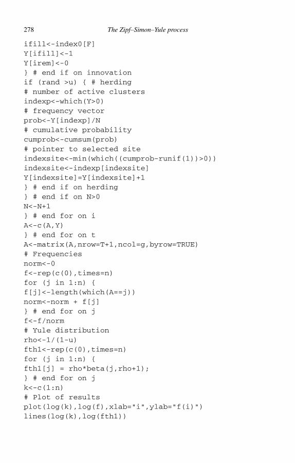
278 The Zipf–Simon–Yule process
ifill<-index0[F]Y[ifill]<-1Y[irem]<-0} # end if on innovationif (rand >u) { # herding# number of active clustersindexp<-which(Y>0)# frequency vectorprob<-Y[indexp]/N# cumulative probabilitycumprob<-cumsum(prob)# pointer to selected siteindexsite<-min(which((cumprob-runif(1))>0))indexsite<-indexp[indexsite]Y[indexsite]=Y[indexsite]+1} # end if on herding} # end if on N>0N<-N+1} # end for on iA<-c(A,Y)} # end for on tA<-matrix(A,nrow=T+1,ncol=g,byrow=TRUE)# Frequenciesnorm<-0f<-rep(c(0),times=n)for (j in 1:n) {f[j]<-length(which(A==j))norm<-norm + f[j]} # end for on jf<-f/norm# Yule distributionrho<-1/(1-u)fth1<-rep(c(0),times=n)for (j in 1:n) {fth1[j] = rho*beta(j,rho+1);} # end for on jk<-c(1:n)# Plot of resultsplot(log(k),log(f),xlab="i",ylab="f(i)")lines(log(k),log(fth1))
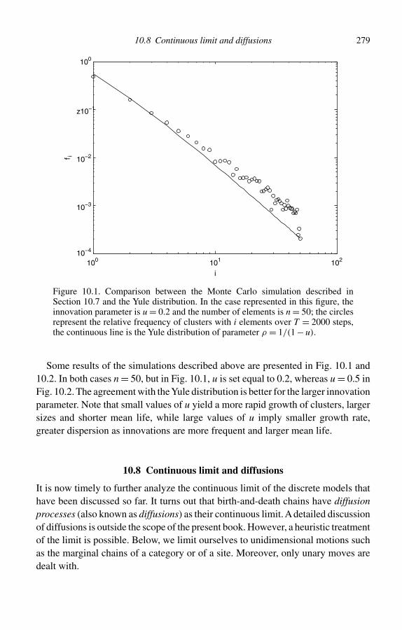
10.8 Continuous limit and diffusions 279
100 101 10210−4
10−3
10−2
z10−1
100
i
f i
Figure 10.1. Comparison between the Monte Carlo simulation described inSection 10.7 and the Yule distribution. In the case represented in this figure, theinnovation parameter is u = 0.2 and the number of elements is n = 50; the circlesrepresent the relative frequency of clusters with i elements over T = 2000 steps,the continuous line is the Yule distribution of parameter ρ = 1/(1 − u).
Some results of the simulations described above are presented in Fig. 10.1 and10.2. In both cases n = 50, but in Fig. 10.1, u is set equal to 0.2, whereas u = 0.5 inFig. 10.2. The agreement with theYule distribution is better for the larger innovationparameter. Note that small values of u yield a more rapid growth of clusters, largersizes and shorter mean life, while large values of u imply smaller growth rate,greater dispersion as innovations are more frequent and larger mean life.
10.8 Continuous limit and diffusions
It is now timely to further analyze the continuous limit of the discrete models thathave been discussed so far. It turns out that birth-and-death chains have diffusionprocesses (also known as diffusions) as their continuous limit. A detailed discussionof diffusions is outside the scope of the present book. However, a heuristic treatmentof the limit is possible. Below, we limit ourselves to unidimensional motions suchas the marginal chains of a category or of a site. Moreover, only unary moves aredealt with.
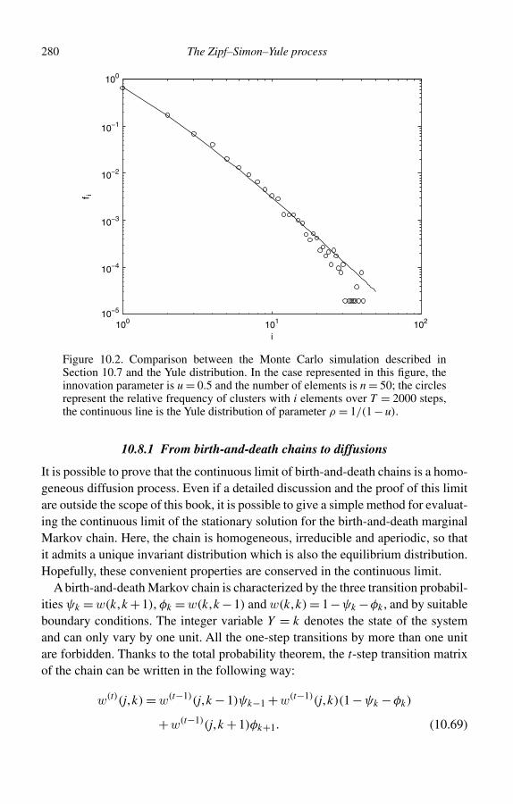
280 The Zipf–Simon–Yule process
100 101 10210−5
10−4
10−3
10−2
10−1
100
i
f i
Figure 10.2. Comparison between the Monte Carlo simulation described inSection 10.7 and the Yule distribution. In the case represented in this figure, theinnovation parameter is u = 0.5 and the number of elements is n = 50; the circlesrepresent the relative frequency of clusters with i elements over T = 2000 steps,the continuous line is the Yule distribution of parameter ρ = 1/(1 − u).
10.8.1 From birth-and-death chains to diffusions
It is possible to prove that the continuous limit of birth-and-death chains is a homo-geneous diffusion process. Even if a detailed discussion and the proof of this limitare outside the scope of this book, it is possible to give a simple method for evaluat-ing the continuous limit of the stationary solution for the birth-and-death marginalMarkov chain. Here, the chain is homogeneous, irreducible and aperiodic, so thatit admits a unique invariant distribution which is also the equilibrium distribution.Hopefully, these convenient properties are conserved in the continuous limit.
A birth-and-death Markov chain is characterized by the three transition probabil-ities ψk = w(k,k +1), φk = w(k,k −1) and w(k,k) = 1−ψk −φk , and by suitableboundary conditions. The integer variable Y = k denotes the state of the systemand can only vary by one unit. All the one-step transitions by more than one unitare forbidden. Thanks to the total probability theorem, the t-step transition matrixof the chain can be written in the following way:
w(t)(j,k) = w(t−1)(j,k − 1)ψk−1 +w(t−1)(j,k)(1 −ψk −φk)
+w(t−1)(j,k + 1)φk+1. (10.69)
10.8 Continuous limit and diffusions 281
In order to connect this chain to diffusion processes, a physical analogy is useful.Assume that Y (t − 1) = k represents the position of a diffusing particle on a one-dimensional lattice. At the next time step t, the particle can jump only to the twonearest-neighbour sites denoted by Y = k − 1 and Y = k + 1 or stay at its currentposition. If x represents the distance between lattice sites and t is the timeinterval between jumps, introducing the probability density p(x, t|x0,0) such thatw(t)(x0,x) = p(x, t|x0,0) x, Equation (10.69) can be re-written as
p(x, t|x0,0) x = p(x − x, t − t|x0,0) x ·ψ(x − x)
+ p(x, t − t|x0,0) x · (1 −ψ(x)−φ(x))
+ p(x + x, t − t|x0,0) x ·φ(x + x), (10.70)
where p(x, t|x0,0) x replaces w(t)(j,k). Note that the factor x can be simplifiedleading to
p(x, t|x0,0) = p(x − x, t − t|x0,0)ψ(x − x)
+ p(x, t − t|x0,0)(1 −ψ(x)−φ(x))
+ p(x + x, t − t|x0,0)φ(x + x). (10.71)
It is now interesting to see what happens if x and t vanish. This cannot bearbitrarily done. First of all, it is necessary to assume that the infinitesimal meanµ(x) and variance σ 2(x) of the process exist, so that
µ(x) = lim t→0
1
t[E((X (t + t)− X (t)|X (t) = x)], (10.72)
and
σ 2(x) = lim t→0
1
t[V((X (t + t)− X (t)|X (t) = x)]. (10.73)
Then, one observes that, if the diffusing particle is in position X (t) = x at time t,the difference X (t + t) − X (t) is equal to x with probability ψ(x), equal to 0with probability 1 −ψ(x)−φ(x) and equal to − x with probability φ(x), so that
E(X (t + t)− X (t)|X (t) = x) = (ψ(x)−φ(x)) x, (10.74)
and
V(X (t + t)− X (t)|X (t) = x) = [ψ(x)+φ(x)− (ψ(x)−φ(x))2]( x)2.(10.75)
282 The Zipf–Simon–Yule process
Comparing Equations (10.74) and (10.75) to (10.72) and (10.73) for finite, butsmall, t, one gets
µ(x) t ≈ (ψ(x)−φ(x)) x, (10.76)
and
σ 2(x) t ≈ [ψ(x)+φ(x)− (ψ(x)−φ(x))2]( x)2. (10.77)
These equations become exact in the so-called diffusive limit, with x → 0 and t → 0, but with the ratio ( x)2/ t = A kept constant (or converging to a constant):
µ(x) = lim x, t→0
(ψ(x)−φ(x)) x
t, (10.78)
and
σ 2(x) = lim x, t→0
[ψ(x)+φ(x)− (ψ(x)−φ(x))2]( x)2
t. (10.79)
Now, replacing
( x)2 = A t, (10.80)
ψ(x) ≈ 1
2A[σ 2(x)+µ(x) x], (10.81)
φ(x) ≈ 1
2A[σ 2(x)−µ(x) x], (10.82)
into Equation (10.71), expanding p(x, t − t|x0,0) and p(x ± x, t − t|x0,0) in aTaylor series around (x, t) as well as µ(x ± x) and σ 2(x ± x) in Taylor seriesaround x, and keeping the terms up to order t (including ( x)2), straightforwardbut tedious calculations lead to the Fokker–Planck equation, also known as theKolmogorov forward equation
∂
∂tp(x, t|x0,0) = − ∂
∂x[µ(x)p(x, t|x0,0)]+ 1
2
∂2
∂x2[σ 2(x)p(x, t|x0,0)]. (10.83)
In particular, in Section 10.9, the stationary solution of Equation (10.83) isderived, coinciding with the continuous limit of the stationary probability ofthe birth-and-death Markov chain. When the stationary condition is reached,p(x) = limt→∞ p(x, t|x0,0), one has
limt→∞
∂
∂tp(x, t|x0,0) = 0, (10.84)
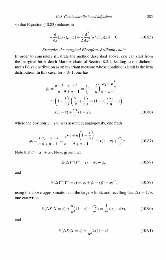
10.8 Continuous limit and diffusions 283
so that Equation (10.83) reduces to
− d
dx[µ(x)p(x)]+ 1
2
d2
dx2[σ 2(x)p(x)] = 0. (10.85)
Example: the marginal Ehrenfest–Brillouin chain
In order to concretely illustrate the method described above, one can start fromthe marginal birth–death Markov chain of Section 8.2.1, leading to the dichoto-mous Pólya distribution as an invariant measure whose continuous limit is the betadistribution. In this case, for n � 1, one has
ψi = n − i
n
α1 + i
θ + n − 1=(
1 − i
n
) α1 + ni
nθ + n − 1
(
1 − i
n
)(α1
n+ i
n
)= (1 − x)
(α1
n+ x)
= x(1 − x)+ α1
n(1 − x), (10.86)
where the position x = i/n was assumed; analogously, one finds
φi = i
n
α2 + n − i
θ + n − 1= i
n
α2 + n
(1 − i
n
)θ + n − 1
x(1 − x)+ α2
nx. (10.87)
Note that θ = α1 +α2. Now, given that
E( Y ∗|Y ∗ = i) = ψi −φi, (10.88)
and
V( Y ∗|Y ∗ = i) = ψi +φi − (ψi −φi)2, (10.89)
using the above approximations in the large n limit, and recalling that x = 1/n,one can write
E( X |X = x) ≈ α1
n2(1 − x)− α2
n2x = 1
n2(α1 − θx), (10.90)
and
V( X |X = x) ≈ 1
n22x(1 − x). (10.91)
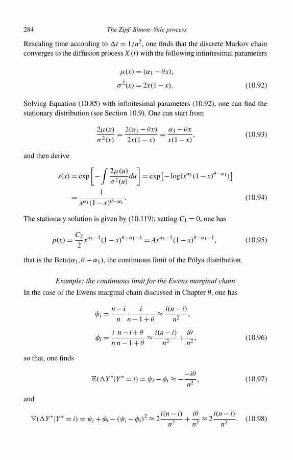
284 The Zipf–Simon–Yule process
Rescaling time according to t = 1/n2, one finds that the discrete Markov chainconverges to the diffusion process X (t) with the following infinitesimal parameters
µ(x) = (α1 − θx),
σ 2(x) = 2x(1 − x). (10.92)
Solving Equation (10.85) with infinitesimal parameters (10.92), one can find thestationary distribution (see Section 10.9). One can start from
2µ(x)
σ 2(x)= 2(α1 − θx)
2x(1 − x)= α1 − θx
x(1 − x), (10.93)
and then derive
s(x) = exp
[−∫
2µ(u)
σ 2(u)du
]= exp
[− log(xα1(1 − x)θ−α1)]
= 1
xα1(1 − x)θ−α1. (10.94)
The stationary solution is given by (10.119); setting C1 = 0, one has
p(x) = C2
2xα1−1(1 − x)θ−α1−1 = Axα1−1(1 − x)θ−α1−1, (10.95)
that is the Beta(α1,θ −α1), the continuous limit of the Pólya distribution.
Example: the continuous limit for the Ewens marginal chain
In the case of the Ewens marginal chain discussed in Chapter 9, one has
ψi = n − i
n
i
n − 1 + θ≈ i(n − i)
n2,
φi = i
n
n − i + θ
n − 1 + θ≈ i(n − i)
n2+ iθ
n2, (10.96)
so that, one finds
E( Y ∗|Y ∗ = i) = ψi −φi ≈ −−iθ
n2, (10.97)
and
V( Y ∗|Y ∗ = i) = ψi +φi − (ψi −φi)2 ≈ 2
i(n − i)
n2+ iθ
n2≈ 2
i(n − i)
n2. (10.98)
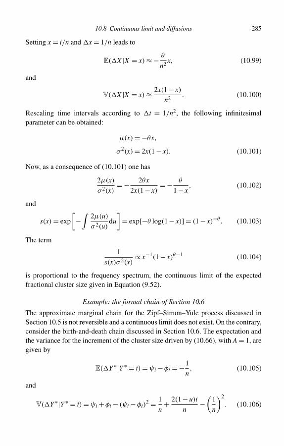
10.8 Continuous limit and diffusions 285
Setting x = i/n and x = 1/n leads to
E( X |X = x) ≈ − θ
n2x, (10.99)
and
V( X |X = x) ≈ 2x(1 − x)
n2. (10.100)
Rescaling time intervals according to t = 1/n2, the following infinitesimalparameter can be obtained:
µ(x) = −θx,
σ 2(x) = 2x(1 − x). (10.101)
Now, as a consequence of (10.101) one has
2µ(x)
σ 2(x)= − 2θx
2x(1 − x)= − θ
1 − x, (10.102)
and
s(x) = exp
[−∫
2µ(u)
σ 2(u)du
]= exp[−θ log(1 − x)] = (1 − x)−θ . (10.103)
The term
1
s(x)σ 2(x)∝ x−1(1 − x)θ−1 (10.104)
is proportional to the frequency spectrum, the continuous limit of the expectedfractional cluster size given in Equation (9.52).
Example: the formal chain of Section 10.6
The approximate marginal chain for the Zipf–Simon–Yule process discussed inSection 10.5 is not reversible and a continuous limit does not exist. On the contrary,consider the birth-and-death chain discussed in Section 10.6. The expectation andthe variance for the increment of the cluster size driven by (10.66), with A = 1, aregiven by
E( Y ∗|Y ∗ = i) = ψi −φi = −1
n, (10.105)
and
V( Y ∗|Y ∗ = i) = ψi +φi − (ψi −φi)2 = 1
n+ 2(1 − u)i
n−(
1
n
)2
. (10.106)
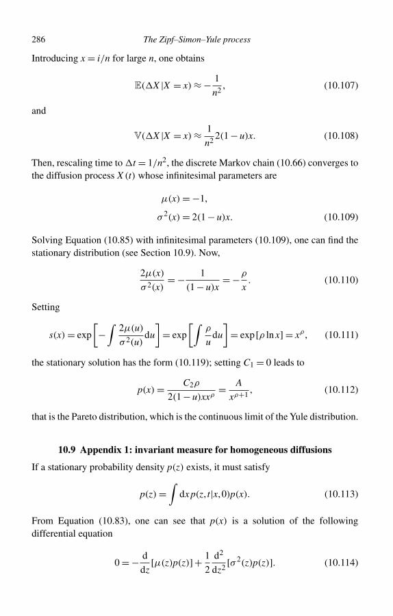
286 The Zipf–Simon–Yule process
Introducing x = i/n for large n, one obtains
E( X |X = x) ≈ − 1
n2, (10.107)
and
V( X |X = x) ≈ 1
n22(1 − u)x. (10.108)
Then, rescaling time to t = 1/n2, the discrete Markov chain (10.66) converges tothe diffusion process X (t) whose infinitesimal parameters are
µ(x) = −1,
σ 2(x) = 2(1 − u)x. (10.109)
Solving Equation (10.85) with infinitesimal parameters (10.109), one can find thestationary distribution (see Section 10.9). Now,
2µ(x)
σ 2(x)= − 1
(1 − u)x= −ρ
x. (10.110)
Setting
s(x) = exp
[−∫
2µ(u)
σ 2(u)du
]= exp
[∫ρ
udu
]= exp[ρ ln x] = xρ , (10.111)
the stationary solution has the form (10.119); setting C1 = 0 leads to
p(x) = C2ρ
2(1 − u)xxρ= A
xρ+1, (10.112)
that is the Pareto distribution, which is the continuous limit of the Yule distribution.
10.9 Appendix 1: invariant measure for homogeneous diffusions
If a stationary probability density p(z) exists, it must satisfy
p(z) =∫
dx p(z, t|x,0)p(x). (10.113)
From Equation (10.83), one can see that p(x) is a solution of the followingdifferential equation
0 = − d
dz[µ(z)p(z)]+ 1
2
d2
dz2[σ 2(z)p(z)]. (10.114)
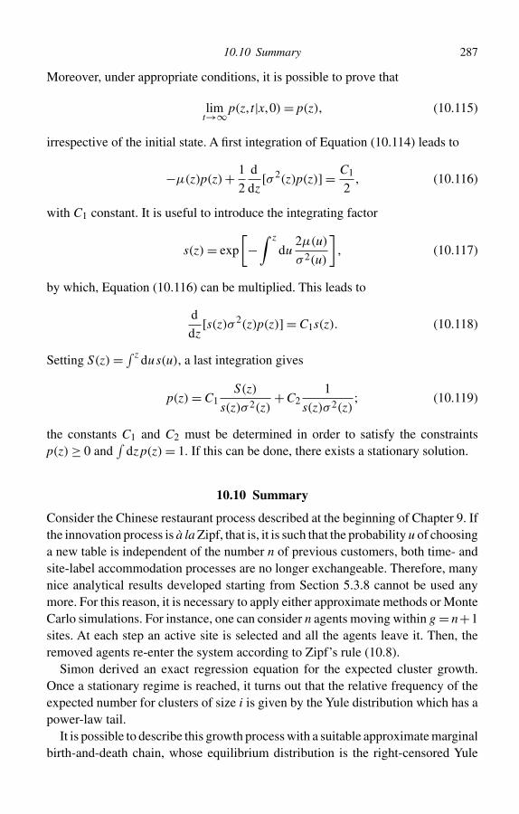
10.10 Summary 287
Moreover, under appropriate conditions, it is possible to prove that
limt→∞p(z, t|x,0) = p(z), (10.115)
irrespective of the initial state. A first integration of Equation (10.114) leads to
−µ(z)p(z)+ 1
2
d
dz[σ 2(z)p(z)] = C1
2, (10.116)
with C1 constant. It is useful to introduce the integrating factor
s(z) = exp
[−∫ z
du2µ(u)
σ 2(u)
], (10.117)
by which, Equation (10.116) can be multiplied. This leads to
d
dz[s(z)σ 2(z)p(z)] = C1s(z). (10.118)
Setting S(z) = ∫ z dus(u), a last integration gives
p(z) = C1S(z)
s(z)σ 2(z)+ C2
1
s(z)σ 2(z); (10.119)
the constants C1 and C2 must be determined in order to satisfy the constraintsp(z) ≥ 0 and
∫dz p(z) = 1. If this can be done, there exists a stationary solution.
10.10 Summary
Consider the Chinese restaurant process described at the beginning of Chapter 9. Ifthe innovation process is à la Zipf, that is, it is such that the probability u of choosinga new table is independent of the number n of previous customers, both time- andsite-label accommodation processes are no longer exchangeable. Therefore, manynice analytical results developed starting from Section 5.3.8 cannot be used anymore. For this reason, it is necessary to apply either approximate methods or MonteCarlo simulations. For instance, one can consider n agents moving within g = n+1sites. At each step an active site is selected and all the agents leave it. Then, theremoved agents re-enter the system according to Zipf’s rule (10.8).
Simon derived an exact regression equation for the expected cluster growth.Once a stationary regime is reached, it turns out that the relative frequency of theexpected number for clusters of size i is given by the Yule distribution which has apower-law tail.
It is possible to describe this growth process with a suitable approximate marginalbirth-and-death chain, whose equilibrium distribution is the right-censored Yule
288 The Zipf–Simon–Yule process
distribution. A formal birth- and death-chain can also be written whose equilibriumdistribution is the right-truncated Yule distribution. In both cases, the dynamics ison the size of a cluster.
The final part of this chapter is devoted to the relationship between birth-and-death chain and diffusion processes for the Ehrenfest–Brillouin and Ewens marginalchains. It is also shown that the continuous limit of the formal Zipf-Simon-Yulechain leads to the continuous Pareto distribution.
Further reading
In 1925, G. Udny Yule published his paper on a mathematical theory of evolutionbased on the conclusions of Dr. J.C. Willis
G.U. Yule, A Mathematical Theory of Evolution, Based on the Conclusions of Dr. J.C. Willis,Philosophical Transactions of the Royal Society of London. Series B, Containing Papers ofa Biological Character, 213, 21–87 (1925).
It contains a detailed discussion of what later became known as theYule distribution.Thirty years later, Herbert Simon published his paper discussing a class of skewdistribution functions, where he recovered the Yule distribution in the solution ofhis regression equations
H. Simon, On a Class of Skew Distribution Functions, Biometrika, 42, 425–440 (1955).
These results are critically discussed in two recent papers on which this chapter isbased:
D. Costantini, S. Donadio, U. Garibaldi and P. Viarengo, Herding and Clustering: Ewensvs. Simon–Yule Models, Physica A, 355, 224–231 (2005).
U. Garibaldi, D. Costantini, S. Donadio and P. Viarengo, Herding and Clustering inEconomics: The Yule-Zipf-Simon Model, Computational Economics, 27, 115–134 (2006).
The continuous limit of birth-and-death Markov chains is discussed both in thebook by Cox and Miller:
D.R. Cox and H.D. Miller, The Theory of Stochastic Processes, Wiley, New York (1965).
and in the treatise by Karlin and Taylor:
S. Karlin and H.M. Taylor, A Second Course in Stochastic Processes, Academic Press, NewYork (1981).
This limit leads to diffusion processes (also known as diffusions). A rigorousdiscussion of diffusion can be found in the two volumes written by Rogers andWilliams:
L.C.G. Rogers and D. Williams, Diffusions, Markov Processes and Martingales: Volume 1,Foundations, Cambridge University Press, Cambridge, UK (2000).
L.C.G. Rogers and D. Williams, Diffusions, Markov Processes and Martingales: Volume 2,Itô Calculus, Cambridge University Press, Cambridge, UK (2000).
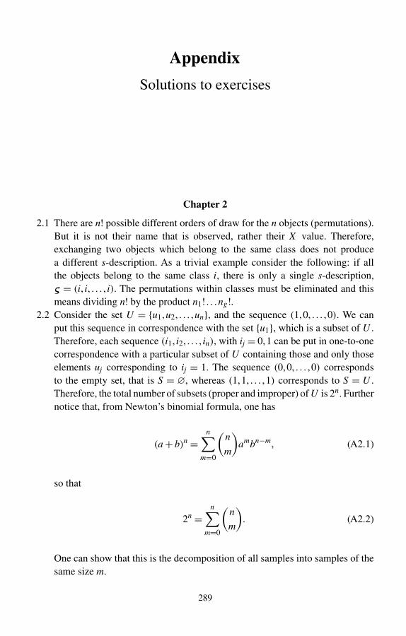
Appendix
Solutions to exercises
Chapter 2
2.1 There are n! possible different orders of draw for the n objects (permutations).But it is not their name that is observed, rather their X value. Therefore,exchanging two objects which belong to the same class does not producea different s-description. As a trivial example consider the following: if allthe objects belong to the same class i, there is only a single s-description,ς = (i, i, . . . , i). The permutations within classes must be eliminated and thismeans dividing n! by the product n1! . . .ng !.
2.2 Consider the set U = {u1,u2, . . . ,un}, and the sequence (1,0, . . . ,0). We canput this sequence in correspondence with the set {u1}, which is a subset of U .Therefore, each sequence (i1, i2, . . . , in), with ij = 0,1 can be put in one-to-onecorrespondence with a particular subset of U containing those and only thoseelements uj corresponding to ij = 1. The sequence (0,0, . . . ,0) correspondsto the empty set, that is S = ∅, whereas (1,1, . . . ,1) corresponds to S = U .Therefore, the total number of subsets (proper and improper) of U is 2n. Furthernotice that, from Newton’s binomial formula, one has
(a + b)n =n∑
m=0
(n
m
)ambn−m, (A2.1)
so that
2n =n∑
m=0
(n
m
). (A2.2)
One can show that this is the decomposition of all samples into samples of thesame size m.
289
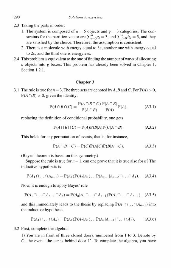
290 Solutions to exercises
2.3 Taking the parts in order:1. The system is composed of n = 5 objects and g = 3 categories. The con-
straints for the partition vector are∑n
i=0 zi = 3, and∑n
i=0 izi = 5, and theyare satisfied by the choice. Therefore, the assumption is consistent.
2. There is a molecule with energy equal to 3ε, another one with energy equalto 2ε, and the third one is energyless.
2.4 This problem is equivalent to the one of finding the number of ways of allocatingn objects into g boxes. This problem has already been solved in Chapter 1,Section 1.2.1.
Chapter 3
3.1 The rule is true for n = 3. The three sets are denoted by A, B and C. For P(A)> 0,P(A ∩ B) > 0, given the identity:
P(A ∩ B ∩ C) = P(A ∩ B ∩ C)
P(A ∩ B)
P(A ∩ B)
P(A)P(A), (A3.1)
replacing the definition of conditional probability, one gets
P(A ∩ B ∩ C) = P(A)P(B|A)P(C|A ∩ B). (A3.2)
This holds for any permutation of events, that is, for instance,
P(A ∩ B ∩ C) = P(C)P(A|C)P(B|A ∩ C). (A3.3)
(Bayes’ theorem is based on this symmetry.)Suppose the rule is true for n−1, can one prove that it is true also for n? The
inductive hypothesis is
P(A1 ∩ . . .∩ An−1) = P(A1)P(A2|A1) . . .P(An−1|An−2 ∩ . . .∩ A1). (A3.4)
Now, it is enough to apply Bayes’ rule
P(A1 ∩ . . .∩ An−1 ∩ An) = P(An|A1 ∩ . . .∩ An−1)P(A1 ∩ . . .∩ An−1), (A3.5)
and this immediately leads to the thesis by replacing P(A1 ∩ . . . ∩ An−1) intothe inductive hypothesis
P(A1 ∩ . . .∩ An) = P(A1)P(A2|A1) . . .P(An|An−1 ∩ . . .∩ A1). (A3.6)
3.2 First, complete the algebra:
1) You are in front of three closed doors, numbered from 1 to 3. Denote byC1 the event ‘the car is behind door 1’. To complete the algebra, you have
Solutions to exercises 291
to introduce Cc1, i.e. ‘the car is not behind door 1’. It is better to distinguish
between door 2 and door 3: hence you also introduce C2 and C3, with themeaning Ci = ‘the car is behind door i’. Now, {Ci}3
i=1 is a decomposition of�, which allows you to freely speak about the positions of the car. The sameprocedure can be applied to your choice: let Di = ‘you say that the car is behinddoor i’. Now Ci and Dj are logically independent, that is they belong to differentdecompositions of �, whereas, for instance, C1 and C2 ∪ C3 have an oppositetruth value; if C1 is true C2 ∪ C3 is false, and if C1 is false, C2 ∪ C3 is true.Now let the quiz master enter the game, let him/her open one door with no carbehind it and let Mi = ‘behind door i there is no car’. Based on the discussionin Example 3.6.3, all a priori possible constituents are then the 27 conjunctions{Di ∩ Cj ∩ Mk ; i, j,k = 1,2,3} describing all possible states of affairs after thequiz master opened one door. Indeed, some of them are impossible (empty),and must be discarded. Thanks to the symmetry of this problem one can justconsider the case wherein D1 = ‘you say that the car is behind door 1’ is true.The following analysis is conditioned on D1 and the constituents are reducedto the following set of nine elements: {Ci ∪ Mj; i, j = 1,2,3}. These elementsare discussed below.1. Ci ∩ M1 = ∅, i = 1,2,3, as the quiz master never opens a door selected by
you; this eliminates 3 elements;2. Ci ∩Mi = ∅, i = 2,3 as the quiz master does not lie, he/she shows an empty
room, and this eliminates 2 more elements.Therefore conditioned on D1, the non-empty constituents are four:1. C1 ∩ M2, C1 ∩ M3, corresponding to a correct guess;2. C2 ∩ M3, C3 ∩ M2, corresponding to a wrong guess.Conditioned on D1, observe that C1 = (C1 ∩ M2) ∪ (C1 ∩ M3), whereas C2 =C2 ∩ M3, and C3 = C3 ∩ M2. In other words, if C2|D1 is sure then M3 is sure,and the same is valid by permuting 2 and 3. In case C1|D1, corresponding toa win, the quiz master has two possible choices, in the other cases he/she canchoose only one door.
2) It is now possible to give probability values to all the non-empty constituents.From Bayes’ theorem, one gets
P(Ci|D1) = P(Ci ∩ D1)/P(D1) = P(D1|Ci)P(Ci)/P(D1). (A3.7)
It is usually assumed that all rooms are equivalent and that this is commonknowledge, leading to the uniform probability assignment P(Ci) = 1/3 for i =1,2,3. Another usual assumption is P(D1|Ci) = P(D1) as no information flowsfrom the chosen room. Therefore, P(Ci|D1) = P(Ci), and the two decomposi-tions {Ci} and {Dj} are not only logically, but also probabilistically independent,
292 Solutions to exercises
and P(Ci ∩ Dj) = P(Ci)P(Dj). For a complete characterization a probabilityvalue must be assumed for P(Mi|D1 ∩C1), that is the choice of the quiz masterwhen the guess is correct. Assuming P(M2|D1 ∩C1) = P(M3|D1 ∩C1) = 1/2,the four constituents have the following probability:1.
P(C1 ∩ M2|D1) = P(C1|D1)P(M2|D1 ∩ C1) = (1/3)(1/2) = 1/6, (A3.8)
P(C1 ∩ M3|D1) = P(C1|D1)P(M3|D1 ∩ C1) = (1/3)(1/2) = 1/6, (A3.9)
corresponding to the right guess, and two door choices for the quiz master;and
2.P(C2 ∩ M3|D1) = P(C2|D1)P(M3|D1 ∩ C2) = (1/3) · 1 = 1/3, (A3.10)
P(C3 ∩ M2|D1) = P(C3|D1)P(M2|D1 ∩ C3) = (1/3) · 1 = 1/3, (A3.11)
corresponding to the two wrong guesses, with only a possible action for thequiz master.
Note that the posterior probability of C1 is equal to the prior:
P(C1|D1) = P(C1 ∩ M2|D1)+P(C1 ∩ M3|D1) = 1/3 = P(C1). (A3.12)
In other words: the winning probability does not change as a consequence ofthe quiz master action!
3) It is true that, after the action of the quiz master, the possibilities reduce from3 to 2 and this is perhaps the reason why many people wrongly believe thatthe quiz master action changes the initial probability of winning from 1/3 to1/2. However, odds change from 1 : 1 : 1 to 1 : 0 : 2 (assuming the quiz masteropens door 2 after your choice of door 1). In other words, if you are allowed tochange your initial choice, changing enhances your odds of winning. In fact,assume that, conditioned on D1, the quiz master opens door 2, meaning that M2
holds true. Then the space reduces to two constituents, C1 ∩ M2 and C3 ∩ M2,whose union is M2. Hence the posterior probability of {Ci}3
i=1 is
P(C1|M2 ∩ D1) = P(C1 ∩ M2|D1)/P(M2|D1) = (1/6)/(1/2) = 1/3,(A3.13)
P(C2|M2 ∩ D1) = 0, (A3.14)
P(C3|M2 ∩ D1) = P(C3 ∩ M2|D1)/P(M2|D1) = (1/3)/(1/2) = 2/3.(A3.15)
As for the meaning of these formulae: given D1, the quiz master chooses M2
or M3 with the same probability, given that C2 and C3 are equiprobable, and if
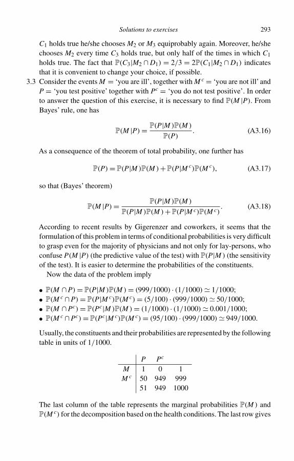
Solutions to exercises 293
C1 holds true he/she chooses M2 or M3 equiprobably again. Moreover, he/shechooses M2 every time C3 holds true, but only half of the times in which C1
holds true. The fact that P(C3|M2 ∩ D1) = 2/3 = 2P(C1|M2 ∩ D1) indicatesthat it is convenient to change your choice, if possible.
3.3 Consider the events M = ‘you are ill’, together with M c = ‘you are not ill’ andP = ‘you test positive’ together with Pc = ‘you do not test positive’. In orderto answer the question of this exercise, it is necessary to find P(M |P). FromBayes’ rule, one has
P(M |P) = P(P|M )P(M )
P(P). (A3.16)
As a consequence of the theorem of total probability, one further has
P(P) = P(P|M )P(M )+P(P|M c)P(M c), (A3.17)
so that (Bayes’ theorem)
P(M |P) = P(P|M )P(M )
P(P|M )P(M )+P(P|M c)P(M c). (A3.18)
According to recent results by Gigerenzer and coworkers, it seems that theformulation of this problem in terms of conditional probabilities is very difficultto grasp even for the majority of physicians and not only for lay-persons, whoconfuse P(M |P) (the predictive value of the test) with P(P|M ) (the sensitivityof the test). It is easier to determine the probabilities of the constituents.
Now the data of the problem imply
• P(M ∩ P) = P(P|M )P(M ) = (999/1000) · (1/1000) 1/1000;• P(M c ∩ P) = P(P|M c)P(M c) = (5/100) · (999/1000) 50/1000;• P(M ∩ Pc) = P(Pc|M )P(M ) = (1/1000) · (1/1000) 0.001/1000;• P(M c ∩ Pc) = P(Pc|M c)P(M c) = (95/100) · (999/1000) 949/1000.
Usually, the constituents and their probabilities are represented by the followingtable in units of 1/1000.
P Pc
M 1 0 1M c 50 949 999
51 949 1000
The last column of the table represents the marginal probabilities P(M ) andP(M c) for the decomposition based on the health conditions. The last row gives
294 Solutions to exercises
the marginal probabilities P(P) and P(Pc) for the decomposition based on thetest results. Coming back to Equation (A3.18), one finds
P(M |P) = P(M ∩ P)
P(M ∩ P)+P(M c ∩ P)= 1
1 + 50≈ 2%, (A3.19)
quite different from P(P|M ) = 99.9%. Given the constituent table, any condi-tional probability can be computed by dividing each entry by the row or columncorresponding to the conditioning event.
Until now, the focus was on the test results for a person. Following a methodtypical of statistical physics, one can build an ensemble which represents theindividual situation by introducing a large number (1000 in this case) of copiesof the unique real system. The number of systems with a certain property isset proportional to the probability of that property in the real system. In theparticular case of this exercise, the table could represent an ensemble of 1000persons that have been tested for the disease and classified with frequenciesproportional to the probabilities. Once the ensemble is built, if the patient ispositive, its probability space is limited to the first column and its probabilityof being ill is given by the number of ill persons in that column divided by thetotal number of persons testing positive.
3.4 Taking the parts in order:1. Let us consider the decomposition of {A(1)
j }j=1,...,g , associated to the descrip-
tion of the first object drawn. The event A(1)j is the disjoint union of all
the sampling sequences (they are n!/(n1! · · ·nj! · · ·ng !)) beginning with j.Their number is given by all sampling sequences belonging to n(j) =(n1, . . . ,nj − 1, . . . ,ng), i.e. (n − 1)!/(n1! · · ·(nj − 1)! · · ·ng !).
Therefore, the probability P(A(1)j ) is
P
(A(1)
j
)= (n − 1)!
n1! · · ·(nj − 1)! · · ·ng !n1! . . .nj! · · ·ng !
n! = nj
n. (A3.20)
The same result holds true for all the other n − 1 objects.2. Now consider A(1)
j ∩ A(2)k , k �= j, which is the disjoint union of all sam-
pling sequences beginning with j,k. Their number is given by all samplingsequences belonging to n(j,k) = (n1, . . . ,nj − 1, . . . ,nk − 1, . . . ,ng) and theyare (n − 2)!/(n1! · · ·(nj − 1)! · · ·(nk − 1)! · · ·ng !). The probability is then
P
(A(1)
j ∩ A(2)k
)= njnk
n(n − 1). (A3.21)
Solutions to exercises 295
Hence, one has
P
(A(1)
j ∩ A(2)k
)= nj
n
nk
n − 1>
nj
n
nk
n= P
(A(1)
j
)P
(A(2)
k
), (A3.22)
for k �= j. Considering j = k, by the same reasoning, one finds
P
(A(1)
j ∩ A(2)j
)= nj
n
nj − 1
n − 1<
nj
n
nj
n= P
(A(1)
j
)P
(A(2)
j
), (A3.23)
that is the joint probability of the two events of the same type is smallerthan the product of the two probabilities. This means that the two events arenegatively correlated.
3. The predictive probability at the second step is
P
(A(2)
k |A(1)j
)=
P
(A(1)
j ∩ A(2)k
)P
(A(1)
j
) , (A3.24)
and the previous results show that
P
(A(2)
k |A(1)j
)= nk − δk,j
n − 1, (A3.25)
where the term δk,j unifies all the possible cases, including k = j. The generalresult in Equation (3.20) can be obtained by repeated application of themultiplication rule leading to
P
(A(m+1)
j |A(1)ω1
. . .A(m)ωm
)= nj − mj
n − m. (A3.26)
In the dichotomous case g = 2, if n = (k,n−k), and m = (h,m−h), Equation(3.20) becomes
P
(A(m+1)
1 |A(1)ω1
. . .A(m)ωm
)= k − h
n − m. (A3.27)
296 Solutions to exercises
Considering the sequence with all k ‘successes’ before the n − k ‘failures’,and applying Equation (A3.27) as well as Bayes’ rule for m = 0, . . . ,n − 1,gives
P({ω}|(k,n − k)) = k
n
k − 1
n − 1· · · 1
n − k + 1
n − k
n − k
n − k − 1
n − k − 1· · · 1
1
= k!n!/(n − k)! =
(n
k
)−1
(A3.28)
as expected.3.5 Assume that there are two alternative and exhaustive hypotheses: H0 =
‘the observed motions have a common cause’, and H1 = ‘the observedmotions are the result of a random assembly of celestial bodies’. Theevidence is E = ‘all the 43 motions are concordant’. Further assumethat before any observation is made P(H0) = P(H1) = 1/2. It meansthat one could bet 1 : 1 on H0. To obtain P(H0|E), one can setP(E|H0) = 1; P(E|H1) can be estimated considering that all motions are inde-pendent and the probability of being in one of the two possible directions withrespect to a chosen body is 1/2. Therefore, P(E|H1) = 2−42. Note that theexponent is 42 and not 43 as one is interested in the relative motion of celestialbodies. Now, using Bayes’ theorem for both hypotheses and dividing:
P(H0|E)
P(H1|E)= P(E|H0)P(H0)
P(E|H1)P(H1)= P(E|H0)
P(E|H1)= 242. (A3.29)
Now 242 = 22+40 = 4 · (210)4 ≥ 4 · (103)4 = 4 · 1012, where 210 = 1024
is approximated by 103. This application of Bayes’ theorem was criticizedbecause the decomposition {H0,H1} is a rough one; also the interpretation ofP(Hi) was challenged. Also the estimate of P(E|H1) is too rough in this case,as the problem is a tridimensional one, whereas, above, the options are reducedto alternatives (that is dichotomous choices).
Moreover, no frequency interpretation is available for P(Hi), and, as a conse-quence, for P(Hi|E). However, an interpretation in terms of betting is possible,as put forward by Laplace himself, as well as a ‘rational belief’ interpretation.In any case, this is a very nice example of plausible reasoning.
Chapter 4
4.1 An equivalence relation xRy, with x,y ∈ A satisfies:1. (identity) any element is in relation with itself, ∀x ∈ A, xRx;2. (symmetry) ∀x,y ∈ A if xRy then yRx; and
Solutions to exercises 297
3. (transitivity) ∀x,y,z ∈ A if xRy and yRz, then xRz.One can represent the relation of the problem as a binary function defined onall ordered couples of the elements of the set as follows: R(ωi,ωj) = 1 if therelation holds true (if ωi and ωj belong to the inverse image of a given label,otherwise R(ωi,ωj) = 0; this is valid for i, j = 1, . . . ,#�. In other words, onesets
R(ωi,ωj) ={
1 if f (ωi) = f (ωj) = b0 if f (ωi) �= f (ωj)
. (A4.1)
Identity and symmetry are obvious, as R(ωi,ωi) = 1; and if R(ωi,ωj) = 1then R(ω2,ω1) = 1. Transitivity holds as R(ωi,ωj) = 1 means f (ωi) = f (ωj),R(ωj,ωk) = 1 means f (ωj) = f (ωk) leading to f (ωi) = f (ωk) finally yieldingR(ωi,ωk) = 1.
4.2 The result straightforwardly follows from the definition; E(a+bX ) =∑x(a+bx)PX (x) = a
∑x PX (x)+ b
∑x xPX (x); therefore
E(a + bX ) = a + bE(X ). (A4.2)
4.3 All the three results are direct consequences of the definition. For the firstquestion, one can use the result of Exercise 4.2.1. One has the following chain of equalities:
V(X ) = E[(X −E(X ))2] = E[X 2 − 2X E(X )+E2(X )] = E(X 2)−E2(X ).(A4.3)
2. The variance is also known as the second centred moment, hence it is notaffected by change of the origin: V(X + a) = V(X ). Indeed, setting Y =X +a, E[Y ] = E[X ]+a, and Y− E[Y ] = X − E[X ], yielding V(Y ) = V(X ).
3. Note that V(bX ) = b2V(X ), as (bX − E[bX ])2 = b2(X − E[X ])2.Hence in synthesis:
V(a + bX ) = b2V(X ) = b2(E(X 2)−E2(X )). (A4.4)
4.4 The first three properties can be proved by showing that the first and the right-hand side of the equations always coincide. As for the intersection, IA∩B(ω)
is 1 if and only if ω ∈ A and ω ∈ B. In this case both IA(ω) and IB(ω) are 1and their product is 1. In all the other possible cases, IA(ω)IB(ω) vanishes.For what concerns the union, its indicator function is one if and only if ω ∈ Aor ω ∈ B. Now, if ω ∈ A and ω /∈ B as well as if ω /∈ A and ω ∈ B, the sumIA(ω) + IB(ω) − IA(ω)IB(ω) is 1 as either IA(ω) or IB(ω) are 1 and the otherterms vanish. If ω ∈ A and ω ∈ B, then again the right-hand side of the equalityis 1 as IA(ω) = 1 and IB(ω) = 1. In the remaining case, ω /∈ A and ω /∈ B, all
298 Solutions to exercises
the three terms vanish. Similarly, in the case of the complement, IAc(ω) is 1 ifω /∈ A and is 0 if ω ∈ A.
The fact that the expected value of the indicator function of an eventA coincides with the probability of A is an immediate consequence of thedefinitions
E(IA(ω)) =∑ω∈�
IA(ω)P(ω) =∑ω∈A
P(ω) = P(A). (A4.5)
Finally, the variance of the indicator function is given by
V(IA) = E[I2A]−P2(A), (A4.6)
but I2A = IA so that
V(IA) = P(A)−P2(A) = P(A)(1 −P(A)). (A4.7)
4.5 Let k = 0,1, . . . ,n represent the composition (k,n − k) of the urn. Introducingthe partition �=∪n
k=0{k}, one has P(X2 = x2|X1 = x1)=∑k P(X2 = x2,k|X1 =x1), and P(X2 = x2,k|X1 = x1)= P(X2 = x2|k,X1 = x1)P(k|X1 = x1) as a conse-quence of the definition of conditional probability. Note that P(X2 = x2|X1 = x1)
is the expected value of P(X2 = x2|k,X1 = x1), but the weights are not P(k),rather P(k|X2 = x1), that is the posterior distribution of the urn composition afterthe observation X1 = x1. In other words, P(X2 = x2|X1 = x1) is the expectedvalue of P(X2 = x2|k,X1 = x1), but the weights are updated due to the occur-rence of X1 = x1. Replacing P(k|X1 = x1) = AP(x1|k)P(k), with A = 1/P(x1),one recovers P(X2 = x2|k,X1 = x1)P(k|X1 = x1) = AP(X2 = x2|k,X1 =x1)P(X1 = x1|k)P(k) = AP(X1 = x1,X2 = x2|k)P(k) leading to (4.73).
Note that P(X2 = x2|k,X1 = x1) depends on the chosen sampling model. Ifsampling is Bernoullian, then one has P(X2 = x2|k,X1 = x1)= P(x2|k) meaningthat the composition of the urn determines the probability whatever X1 = x1; ifsampling is hypergeometric, X1 = x1 is important.Assume that x1 = 1, and that kis the number of type-1 balls: in the Bernoullian case P(X2 = 1|k,X1 = 1)= k/n,whereas in the hypergeometric case P(X2 = 1|k,X1 = 1) = (k −1)/(n−1), andP(X2 = 1|k,X1 = 2) = k/(n − 1).
4.6 The reader should take care to avoid confusing Euler’s beta function
B(a,b) = �(a)�(b)
�(a + b)=∫ 1
0θa−1(1 − θ)b−1dθ (A4.8)
with the beta density
beta(θ ;a,b) = B(a,b)−1θa−1(1 − θ)b−1, (A4.9)
Solutions to exercises 299
defined for θ ∈ [0,1]. Based on the definition of B(a,b), one has that
B(a + 1,b) =∫ 1
0θ · θa−1(1 − θ)b−1dθ , (A4.10)
so that the expected value is
E(�) = B(a,b)−1∫ 1
0θ · θa−1(1 − θ)b−1dθ
= B(a,b)−1B(a + 1,b) = �(a + b)
�(a)�(b)
�(a + 1)�(b)
�(a + b + 1)= a
a + b. (A4.11)
Similarly, the integral for E(�2) is given by
B(a + 2,b) =∫ 1
0θ2 · θa−1(1 − θ)b−1dθ ; (A4.12)
therefore, one obtains
E(�2) = B(a,b)−1∫ 1
0θ2 · θa−1(1 − θ)b−1dθ
= �(a + b)
�(a)�(b)
�(a + 2)�(b)
�(a + b + 2)= a(a + 1)
(a + b + 1)(a + b). (A4.13)
Finally, one arrives at
V(�) = E(�2)−E2(�) = a(a + 1)
(a + b + 1)(a + b)−(
a
a + b
)2
= a(a + 1)(a + b)− a2(a + b + 1)
(a + b + 1)(a + b)2= ab
(a + b + 1)(a + b)2. (A4.14)
Chapter 5
5.1 Assume that the two random variables are defined on the same probabilityspace, and let PX1,X2(x1,x2) be the joint probability distribution defined in
300 Solutions to exercises
Section 4.1.7. One has the following chain of equalities
E(X1 + X2) =∑x1,x2
(x1 + x2)PX1,X2(x1,x2)
=∑x1,x2
(x1PX1,X2(x1,x2)+ x2PX1,X2(x1,x2))
=∑x1,x2
x1PX1,X2(x1,x2)+∑x1,x2
x2PX1,X2(x1,x2)
=∑x1
x1
∑x2
PX1,X2(x1,x2)∑x2
x2
∑x1
PX1,X2(x1,x2)
=∑x1
x1PX1(x1)+∑x2
x2PX2(x2) = E(X1)+E(X1). (A5.1)
The extension of this result to the sum of n random variables can bestraightforwardly obtained by repeated application of the above result.
5.2 Using the properties of the expectation (see Exercise 5.1 above and Exercise5.2), of the variance (see Exercise 5.3) and of the covariance (Equation (4.18)in Section 4.1.7) one has that
V(X1 + X2) = E[(X1 + X2 −E(X1 + X2))2] = E[(X1 + X2)
2]− [E(X1 + X2)]2
= E(X 21 + X 2
2 + 2X1X2)−E2(X1)−E2(X2)− 2E(X1)E(X2)
= E(X 21 )−E2(X1)+E(X 2
2 )−E2(X2)+ 2[E(X1X2)−E(X1)E(X2)]= V(X1)+V(X2)+ 2C(X1,X2). (A5.2)
The extension of this result to n random variables is straightforward as well.In order to represent the square of the sum of n terms, consider an n×n squarematrix, whose entries are the products (Xi − E(Xi))(Xj − E(Xj)). The sumof the n diagonal terms is
∑ni=1 (Xi − E(Xi))
2, the other m(m − 1) terms are∑i �=j (Xi − E(Xi))(Xj − E(Xj)). The expected value of the sum is the sum of
the expected values. Therefore, the covariance matrix is a symmetric matrixwith variances on the diagonal and covariances out of the diagonal.
5.3 The random variable I (k)i I (k)
j differs from zero only when Xi = k and Xj = k,in which case it takes the value 1; in all the other cases it is 0. Therefore, oneimmediately gets
E(I (k)i I (k)
j ) = 1 ·P(Xi = k,Xj = k)+ 0 · · · · = P(Xi = k,Xj = k). (A5.3)
5.4 There is not a unique solution to this problem and there may be severalmethods of optimizing the code for the simulation of Pólya processes. The
Solutions to exercises 301
code below uses the predictive probability to create a dichotomous Pólyasequence, calculates the random walk as a function of m and then plots theresult. The program is written in R, which is a free software environmentfor statistical computing and graphics. The software can be retrieved fromhttp://www.r-project.org.
# Program polyarw.R
n <-1000 # number of iterations
alpha0 <- 10 # parameter of category 0 (failure)
alpha1 <- 10 # parameter of category 1 (success)
alpha <- alpha0 + alpha1 # parameter alpha
m0 <- 0 # number of failures
m1 <- 0 # number of successes
X <- rep(c(0), times=n) # defining the vector of jumps
for (m in 0:n-1) { # main cycle
if ( runif(1) < (alpha1+m1)/(alpha+m)){ # predictive probability
# for success
X[m+1] <-1 # upward jump
m1<- m1+1 # update of success number
} # end if
else { # else failure
X[m+1]<--1 # downward jump
m0 <- m0+1 # update of failure number
} # end else
} # end for
S <- cumsum(X) # implementing eq. (5.160)
t <- c(1:n) # time steps
plot(t,S,xlab="m",ylab="S(m)") # plot
In Fig. A5.1, a simulation for the case α0 = 1, α1 = 1 is plotted. Figure A5.2contains a realization of the Pólya random walk for α0 = α1 = 10. Finally, Fig.A5.3 shows a simulation of α0 = α1 = 100. Even if the a priori probabilities docoincide in the three cases p0 = p1 = 1/2, the behaviour of the random walkis very different. For small α (Fig. A5.1), it is almost deterministic. The initialchoice gives a great advantage to the selected category (see the discussionin Section 5.6.2). In Fig. A5.3, by direct visual inspection, one can see thatthe behaviour of the Pólya random walk for α0 = α1 = 100 is very close tothat of a standard random walk where the variables X (m) are independent andidentically distributed with equal probability of success and failure (as in cointosses). It would not be easy for a statistician to distinguish between the casespresented in Fig. A5.3 and A5.4, the latter being a realization of a standardrandom walk.
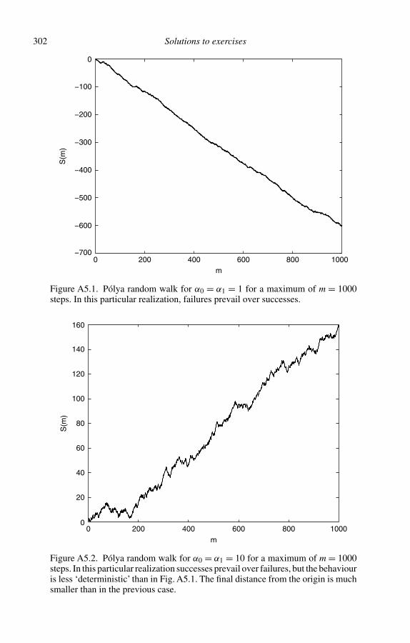
302 Solutions to exercises
0 200 400 600 800 1000−700
−600
−500
−400
−300
−200
−100
0
m
S(m
)
Figure A5.1. Pólya random walk for α0 = α1 = 1 for a maximum of m = 1000steps. In this particular realization, failures prevail over successes.
0 200 400 600 800 10000
20
40
60
80
100
120
140
160
m
S(m
)
Figure A5.2. Pólya random walk for α0 = α1 = 10 for a maximum of m = 1000steps. In this particular realization successes prevail over failures, but the behaviouris less ‘deterministic’ than in Fig. A5.1. The final distance from the origin is muchsmaller than in the previous case.
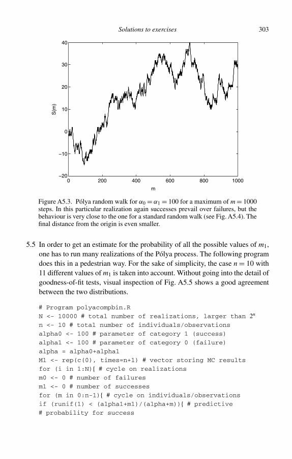
Solutions to exercises 303
0 200 400 600 800 1000−20
−10
0
10
20
30
40
m
S(m
)
Figure A5.3. Pólya random walk for α0 = α1 = 100 for a maximum of m = 1000steps. In this particular realization again successes prevail over failures, but thebehaviour is very close to the one for a standard random walk (see Fig. A5.4). Thefinal distance from the origin is even smaller.
5.5 In order to get an estimate for the probability of all the possible values of m1,one has to run many realizations of the Pólya process. The following programdoes this in a pedestrian way. For the sake of simplicity, the case n = 10 with11 different values of m1 is taken into account. Without going into the detail ofgoodness-of-fit tests, visual inspection of Fig. A5.5 shows a good agreementbetween the two distributions.
# Program polyacompbin.R
N <- 10000 # total number of realizations, larger than 2n
n <- 10 # total number of individuals/observations
alpha0 <- 100 # parameter of category 1 (success)
alpha1 <- 100 # parameter of category 0 (failure)
alpha = alpha0+alpha1
M1 <- rep(c(0), times=n+1) # vector storing MC results
for (i in 1:N){ # cycle on realizations
m0 <- 0 # number of failures
m1 <- 0 # number of successes
for (m in 0:n-1){ # cycle on individuals/observations
if (runif(1) < (alpha1+m1)/(alpha+m)){ # predictive
# probability for success
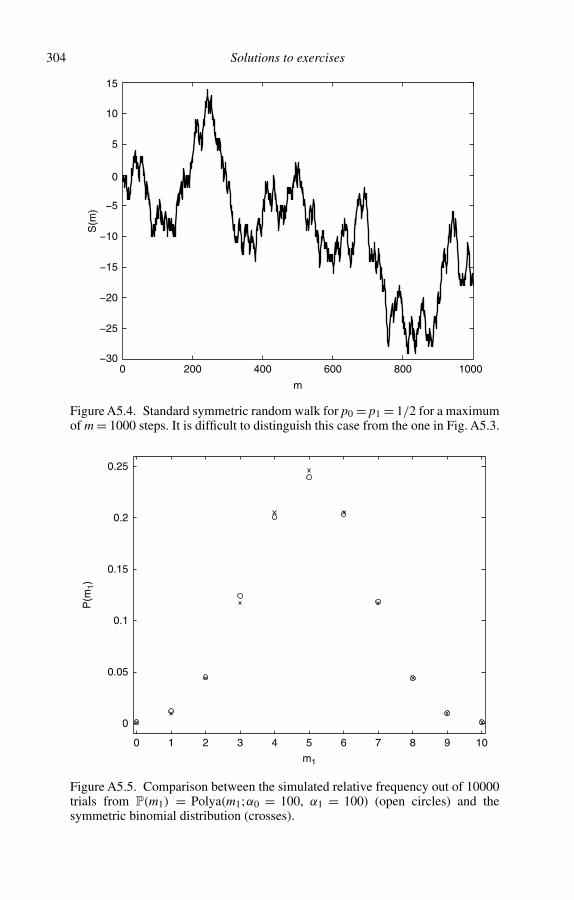
304 Solutions to exercises
0 200 400 600 800 1000−30
−25
−20
−15
−10
−5
0
5
10
15
m
S(m
)
Figure A5.4. Standard symmetric random walk for p0 = p1 = 1/2 for a maximumof m = 1000 steps. It is difficult to distinguish this case from the one in Fig. A5.3.
0 1 2 3 4 5 6 7 8 9 10
0
0.05
0.1
0.15
0.2
0.25
m1
P(m
1)
Figure A5.5. Comparison between the simulated relative frequency out of 10000trials from P(m1) = Polya(m1;α0 = 100, α1 = 100) (open circles) and thesymmetric binomial distribution (crosses).
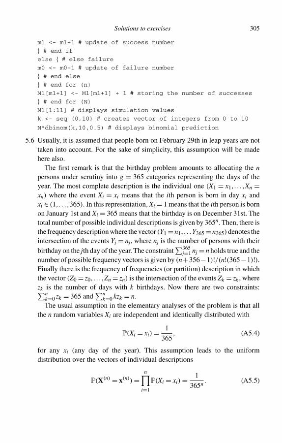
Solutions to exercises 305
m1 <- m1+1 # update of success number
} # end if
else { # else failure
m0 <- m0+1 # update of failure number
} # end else
} # end for (n)
M1[m1+1] <- M1[m1+1] + 1 # storing the number of successes
} # end for (N)
M1[1:11] # displays simulation values
k <- seq (0,10) # creates vector of integers from 0 to 10
N*dbinom(k,10,0.5) # displays binomial prediction
5.6 Usually, it is assumed that people born on February 29th in leap years are nottaken into account. For the sake of simplicity, this assumption will be madehere also.
The first remark is that the birthday problem amounts to allocating the npersons under scrutiny into g = 365 categories representing the days of theyear. The most complete description is the individual one (X1 = x1, . . . ,Xn =xn) where the event Xi = xi means that the ith person is born in day xi andxi ∈ (1, . . . ,365). In this representation, Xi = 1 means that the ith person is bornon January 1st and Xi = 365 means that the birthday is on December 31st. Thetotal number of possible individual descriptions is given by 365n. Then, there isthe frequency description where the vector (Y1 = n1, . . .Y365 = n365)denotes theintersection of the events Yj = nj, where nj is the number of persons with theirbirthday on the jth day of the year. The constraint
∑365j=1 nj = n holds true and the
number of possible frequency vectors is given by (n+356−1)!/(n!(365−1)!).Finally there is the frequency of frequencies (or partition) description in whichthe vector (Z0 = z0, . . . ,Zn = zn) is the intersection of the events Zk = zk , wherezk is the number of days with k birthdays. Now there are two constraints:∑n
k=0 zk = 365 and∑n
k=0 kzk = n.The usual assumption in the elementary analyses of the problem is that all
the n random variables Xi are independent and identically distributed with
P(Xi = xi) = 1
365, (A5.4)
for any xi (any day of the year). This assumption leads to the uniformdistribution over the vectors of individual descriptions
P(X(n) = x(n)) =n∏
i=1
P(Xi = xi) = 1
365n. (A5.5)
306 Solutions to exercises
Now, due to exchangeability, using Equation (4.59) leads to
P(Y(n) = n) = n!n1! . . .n356!P(X(n) = x(n)) = n!
n1! . . .n356!1
365n. (A5.6)
Not only are the individual variables exchangeable, but also the frequencies,all the days being on a par. Therefore, a second application of Equation (4.59)yields
P(Z(n) = z(n)) = 365!z0! . . .zn!P(Y(n) = n(n)), (A5.7)
as in Equation (5.72). Applying (5.71) also, one gets
P(Z(n) = z(n)) = 365!z0! . . .zn!
n!(0!z0) · . . . · (n!zn)
1
365n. (A5.8)
Equation (A5.8) can be used to answer all the questions related to birthdaycoincidences. For instance, the probability of no common birthday in a groupof n persons means that Z1 = n and Z0 = 365 − n, all the other Zi being 0. Infact, this is satisfied by any frequency vector including n times 1 (for the daysof the n different birthdays) and 365 − n times 0 for the other days. Therefore,one is led to insert the partition vector Z(n) = (365−n,n,0, . . . ,0) into Equation(A5.8)
P(365 − n,n,0, . . . ,0) = 365!(365 − n)!n!n! 1
365n= 365!
(365 − n)!1
365n. (A5.9)
The event at least one common birthday is the complement of no common birth-day and its probability is just 1−P(365−n,n,0, . . . ,0). This answers the initialquestion.
This solution can be found with more elementary methods, as well. However,Equation (A5.8) can be used to solve other problems. For instance, considerthe probability of the event exactly two birthdays coincide meaning that all theother birthdays are on different days of the year. This means that the frequencydescription has ni = 2 for 1 value of i, nj = 1 for n − 2 values of j and nk = 0for 365−n+1 values of k because only n−1 days are birthdays. This leads tothe partition vector Z(n) = (365 − n + 1,n − 2,1,0 . . . ,0) whose probability is
P(365 − n + 1,n − 2,1,0 . . . ,0) = 365!(365 − n + 1)!(n − 2)!1!
n!2!
1
365n. (A5.10)
Solutions to exercises 307
In particular, for n ≥ 23, it is convenient to bet 1:1 on the presence of a commonbirthday at least.
Chapter 6
6.1 Solution of case a)Note that β = 0 is associated to a deterministic system following the cyclea → b → c → a with probability 1 forever. Then the answer to point 1 isyes, as all states are persistent, the chain is periodic (point 2), and the invariantdistribution (point 3) is π = (1/3,1/3,1/3), which is also the limiting frequencydistribution (point 4). In fact, considering blocks of three steps, each stateoccurs with the same frequency, and in the long run the initial steps, whateverthey are, do not matter for the relative visiting frequency. That the invariantdistribution is π = (1/3,1/3,1/3) can be shown by building an ensemble ofsystems (three are sufficient), one starting from x0 = a, one from x0 = b andone from x0 = c. In the ‘ensemble’ representation, very common in statisticalphysics, the probability of a state is given by the number of systems in that statedivided by the total number of systems.At the second step, all the systems makea clockwise step, and the number of systems in any state is 1 again. If one is notconfident regarding intuition, π is the solution of π = π × W. The answer topoint 5 is negative; indeed, given x0 = a then P(3t) = δ(x,a), P(3t+1) = δ(x,b),and P(3t+2) = δ(x,c), where δ(x, i) is the degenerate probability distributionall concentrated on the ith state, i.e. the probability of state i is 1. This simpleexample illustrates the root of ergodic properties in physics. If the state space isfinite and the dynamics is deterministic the motion is periodic on all persistentstates. The relative frequency of visits converges to the invariant distribution,therefore, instead of taking the time average over the whole trajectory, one canuse the ‘ensemble average’ on π , which is necessarily uniform. Building anensemble proportional to π is an artificial device to introduce a distribution thatthe deterministic dynamics leaves invariant. But one knows that any particularsystem whose initial conditions are known cannot be described by π in thelong run. As for point 6, even if the ensembles were described by the invariantπ = (1/3,1/3,1/3), each system of the ensemble moves clockwise for sure,whereas the backward movie is always counterclockwise. Here, there is noreversibility and no detailed balance.Solution of case b)Now, consider the case β = 1. If the chain reaches state a, it stops thereforever, and a is said to be an equilibrium state in a physics sense. Giventhat all states communicate with a, sooner or later the system stops there.In this simple case, after two steps, one is sure that the system is in a.
308 Solutions to exercises
Then, the limiting and the equilibrium distribution exist in some sense, as,for t ≥ 2, for any initial state P(Xt = j) = δ(j,a), but it is not positive(regular) on all states. States b and c are not persistent (they are called tran-sient) and the chain is reducible. There is no reversibility and no detailedbalance.Solution of case c)In order to fix ideas, let β = 1/2. The possibility of not immediately leavinga state destroys the periodicity of the chain. In fact, W(4) is positive. A littlethought is enough to understand that, in the long run, state a is visited twicemore than states b and c, which, in turn, have the same number of visits. Hence,the limiting visiting frequency distribution is (1/2,1/4,1/4). This result canbe confirmed by solving the Markov equation π = π × W. The chain beingaperiodic, it reaches the limiting distribution π = (1/2,1/4,1/4) after 42 stepswithin 3-digit precision, whatever the initial state. When the chain becomesstationary, the total balance between entering and exiting probabilities vanishes.For instance πb = πa/2 − πb = 0, that is at each step the mass πa/2 entersfrom state a and compensates the mass πb which leaves for state c. Detailedbalance does not hold: in fact, the backward movie is essentially different fromthe direct one. Then there is no reversibility and no detailed balance.
6.4 First note that the events {|X − E(X )| ≥ δ} and {(X − E(X ))2 ≥ δ2} coincide.If VX denotes the set of allowed values of X , one has that
V(X )
δ2=∑
x∈VX
(x −E(X ))2
δ2P(X = x)
=∑
(x−E(X ))2≥δ2
(x −E(X ))2
δ2P(X = x)+
∑(x−E(X ))2<δ2
(x −E(X ))2
δ2P(X = x)
≥∑
(x−E(X ))2≥δ2
(x −E(X ))2
δ2P(X = x) =
∑|x−E(X )|≥δ
(x −E(X ))2
δ2P(X = x)
≥∑
|x−E(X )|≥δ
P(X = x) = P(|X −E(X )| ≥ δ), (A6.1)
where the first equality is the definition of variance, whereas the second equalityis the division of the sum into complementary terms; the first inequality isdue to the fact that all the terms added in the variance are non-negative; thethird equality uses the coincidence discussed above; the second inequality is aconsequence of the fact that, for the summands, one has (x − E(X ))/δ2 ≥ 1;finally, the last equality is by definition.
Solutions to exercises 309
6.5 In order to solve this problem, one has to find a normalized left eigenvector ofW with eigenvalue 1. This leads to the following linearly dependent equations
π1 = 1
3π1 + 3
4π2, (A6.2)
π2 = 2
3π1 + 1
4π2, (A6.3)
corresponding to
π1 = 9
8π2. (A6.4)
Imposing the normalization condition leads to
9
8π2 +π2 = 1, (A6.5)
so that π1 = 9/17 and π2 = 8/17 give the invariant probabilities of state 1 and2, respectively, which are also the equilibrium ones, being the chain irreversibleand aperiodic.
6.6 A little algebra shows that
W(2) = W2 =(
0.611 0.3890.438 0.563
),
W(5) = W5 =(
0.524 0.4770.536 0.464
),
W(10) = W10 =(
0.530 0.4710.529 0.471
).
These results can be compared with π1 = 9/17 0.529 and π2 = 8/17 0.471.6.7 It turns out that
W2k =(
1 00 1
),
and
W2k−1 =(
0 11 0
),
for any integer k ≥ 1. Therefore the powers of this matrix do not converge.
Chapter 7
7.1 Let k denote the number of fleas on the left dog and n − k the number of fleason the right dog. Here, n = 4 and k can vary from 0 to 4. If Y(4)
0 = (0,4), then
310 Solutions to exercises
one has k0 = 0, and D1,D2 are forced to be moves from left to right, therefore,one has Y(2) = (0,2) for sure. There is 1 path C1,C2 leading to k = 2, the pathsC1,C2 leading to k = 1 are 2, and 1 returning to k = 0. Therefore, the first rowof the binary move matrix W(2) is b0j = (1/4,1/2,1/4,0,0). If k = 1, that is
Y(4)0 = (1,3), there are three possible transitions D1,D2, with probability
P(D1 = r,D2 = r) = (3/4) · (2/3) = 1/2P(D1 = r,D2 = l) = (1/4) · (3/3) = 1/4P(D1 = l,D2 = r) = (3/4) · (1/3) = 1/4
, (A7.1)
where r denotes a move to the right and l a move to the left. Note that D1 = r,D2 = r brings us to Y(2) = (1,1), and the uniformity of C1,C2 gives probability(1/4,1/2,1/4) to the final states (1,3), (2,2), (3,1), respectively. Both D1 =r,D2 = l and D1 = l,D2 = r bring us to Y(2) = (0,2), which ends in (0,4),(1,3), (2,2)with probability (1/4,1/2,1/4). Then grouping the distinct patternsto each final vector, one finds b10 = (1/2)(1/4) = 1/8, b11 = (1/2)(1/2) +(1/2)(1/4) = 3/8, b12 = (1/2)(1/4)+ (1/2)(1/2) = 3/8, b13 = (1/2)(1/4) =1/8, b14 = 0. Note that this very cumbersome calculation is highly simplifiedby the independent and symmetric creation terms, and by the small size ofthe population (n = 4). Instead of going on with a detailed description of thetransitions, the matrix can be completed using the detailed balance Equations(7.113) and (7.114). First, one can check that the previous results are correct. Forinstance b10/b01 = (1/8)/(1/2) = 1/4, which is exactly the ratio π1/π4, whenπk = Bin(k|4,1/2). Considering that the symmetry implies that bi,j = b4−i,4−j,the third row can be calculated from b2,j = bj,2πj/π2. Therefore, one getsb2,0 = b0,2π0/π2 = (1/4)(1/6) = 1/24, b2,1 = b1,2π1/π2 = (3/8)(4/6) = 1/4,b2,3 = b3,2π3/π2 = (3/8)(4/6) = 1/4 and b2,4 = b4,2π4/π2 = (1/4)(1/6) =1/24, where b3,2 = b1,2, b4,2 = b0,2 and b2,2 = 1 − 1/12 − 1/2 = 5/12 bynormalization. Finally, the matrix W(2) = { bij} is the following
W(2) =
1/4 1/2 1/4 0 01/8 3/8 3/8 1/8 0
1/24 6/24 10/24 6/24 1/240 1/8 3/8 3/8 1/80 0 1/4 1/2 1/4
, (A7.2)
which is different from both the unary matrix (6.30), and from its square W(2).However, the approach to equilibrium is such that W
(t)(2) is equal to W(∞) up to
3-digit precision for t = 13 (instead of t = 30).As for the comparison of the two chains, with transition matrices W and W(2)
corresponding to unary/binary moves (m = 1 versus m = 2), it is interesting
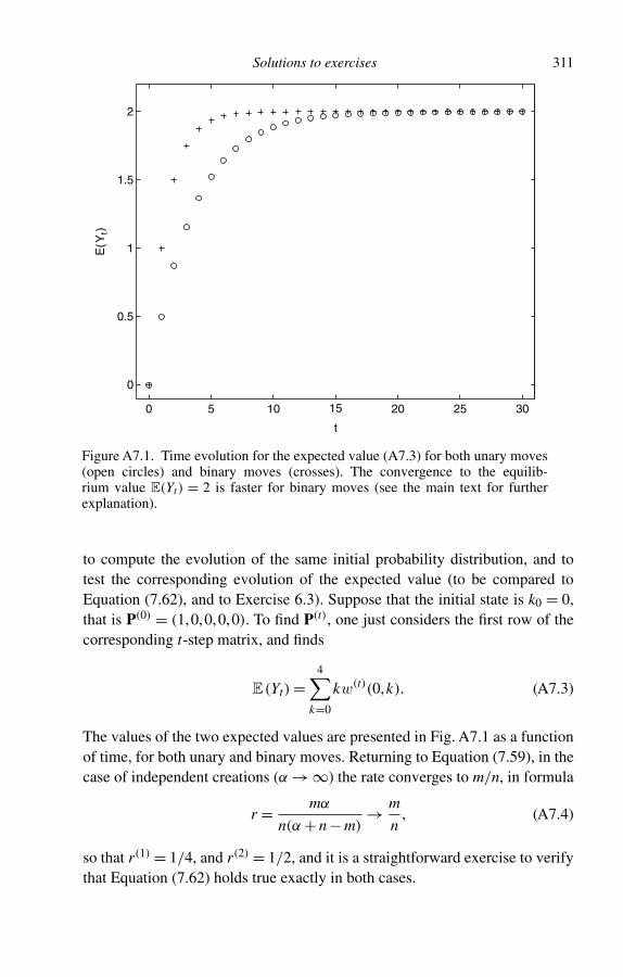
Solutions to exercises 311
0 5 10 15 20 25 30
0
0.5
1
1.5
2
t
E(Y
t)
Figure A7.1. Time evolution for the expected value (A7.3) for both unary moves(open circles) and binary moves (crosses). The convergence to the equilib-rium value E(Yt) = 2 is faster for binary moves (see the main text for furtherexplanation).
to compute the evolution of the same initial probability distribution, and totest the corresponding evolution of the expected value (to be compared toEquation (7.62), and to Exercise 6.3). Suppose that the initial state is k0 = 0,that is P(0) = (1,0,0,0,0). To find P(t), one just considers the first row of thecorresponding t-step matrix, and finds
E(Yt) =4∑
k=0
kw(t)(0,k). (A7.3)
The values of the two expected values are presented in Fig. A7.1 as a functionof time, for both unary and binary moves. Returning to Equation (7.59), in thecase of independent creations (α → ∞) the rate converges to m/n, in formula
r = mα
n(α + n − m)→ m
n, (A7.4)
so that r(1) = 1/4, and r(2) = 1/2, and it is a straightforward exercise to verifythat Equation (7.62) holds true exactly in both cases.
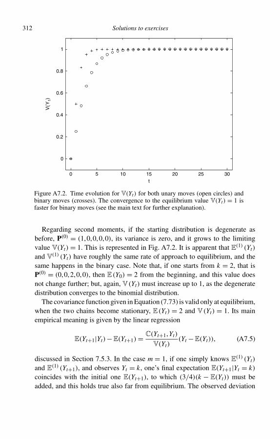
312 Solutions to exercises
0 5 10 15 20 25 30
0
0.2
0.4
0.6
0.8
1
t
V(Y
t)
Figure A7.2. Time evolution for V(Yt) for both unary moves (open circles) andbinary moves (crosses). The convergence to the equilibrium value V(Yt) = 1 isfaster for binary moves (see the main text for further explanation).
Regarding second moments, if the starting distribution is degenerate asbefore, P(0) = (1,0,0,0,0), its variance is zero, and it grows to the limitingvalue V(Yt) = 1. This is represented in Fig. A7.2. It is apparent that E(1) (Yt)
and V(1) (Yt) have roughly the same rate of approach to equilibrium, and thesame happens in the binary case. Note that, if one starts from k = 2, that isP(0) = (0,0,2,0,0), then E(Y0) = 2 from the beginning, and this value doesnot change further; but, again, V(Yt) must increase up to 1, as the degeneratedistribution converges to the binomial distribution.
The covariance function given in Equation (7.73) is valid only at equilibrium,when the two chains become stationary, E(Yt) = 2 and V(Yt) = 1. Its mainempirical meaning is given by the linear regression
E(Yt+1|Yt)−E(Yt+1) = C(Yt+1,Yt)
V(Yt)(Yt −E(Yt)), (A7.5)
discussed in Section 7.5.3. In the case m = 1, if one simply knows E(1) (Yt)
and E(1) (Yt+1), and observes Yt = k, one’s final expectation E(Yt+1|Yt = k)
coincides with the initial one E(Yt+1), to which (3/4)(k − E(Yt)) must beadded, and this holds true also far from equilibrium. The observed deviation
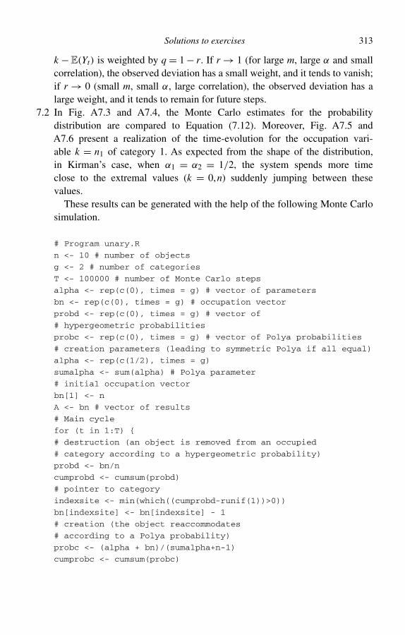
Solutions to exercises 313
k − E(Yt) is weighted by q = 1 − r. If r → 1 (for large m, large α and smallcorrelation), the observed deviation has a small weight, and it tends to vanish;if r → 0 (small m, small α, large correlation), the observed deviation has alarge weight, and it tends to remain for future steps.
7.2 In Fig. A7.3 and A7.4, the Monte Carlo estimates for the probabilitydistribution are compared to Equation (7.12). Moreover, Fig. A7.5 andA7.6 present a realization of the time-evolution for the occupation vari-able k = n1 of category 1. As expected from the shape of the distribution,in Kirman’s case, when α1 = α2 = 1/2, the system spends more timeclose to the extremal values (k = 0,n) suddenly jumping between thesevalues.
These results can be generated with the help of the following Monte Carlosimulation.
# Program unary.R
n <- 10 # number of objects
g <- 2 # number of categories
T <- 100000 # number of Monte Carlo steps
alpha <- rep(c(0), times = g) # vector of parameters
bn <- rep(c(0), times = g) # occupation vector
probd <- rep(c(0), times = g) # vector of
# hypergeometric probabilities
probc <- rep(c(0), times = g) # vector of Polya probabilities
# creation parameters (leading to symmetric Polya if all equal)
alpha <- rep(c(1/2), times = g)
sumalpha <- sum(alpha) # Polya parameter
# initial occupation vector
bn[1] <- n
A <- bn # vector of results
# Main cycle
for (t in 1:T) {
# destruction (an object is removed from an occupied
# category according to a hypergeometric probability)
probd <- bn/n
cumprobd <- cumsum(probd)
# pointer to category
indexsite <- min(which((cumprobd-runif(1))>0))
bn[indexsite] <- bn[indexsite] - 1
# creation (the object reaccommodates
# according to a Polya probability)
probc <- (alpha + bn)/(sumalpha+n-1)
cumprobc <- cumsum(probc)
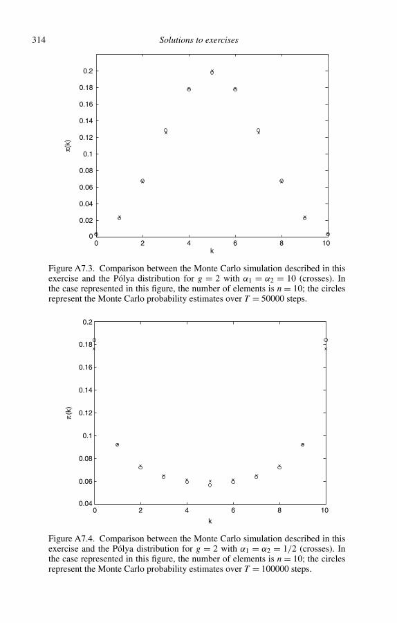
314 Solutions to exercises
0 2 4 6 8 100
0.02
0.04
0.06
0.08
0.1
0.12
0.14
0.16
0.18
0.2
k
π(k)
Figure A7.3. Comparison between the Monte Carlo simulation described in thisexercise and the Pólya distribution for g = 2 with α1 = α2 = 10 (crosses). Inthe case represented in this figure, the number of elements is n = 10; the circlesrepresent the Monte Carlo probability estimates over T = 50000 steps.
0 2 4 6 8 100.04
0.06
0.08
0.1
0.12
0.14
0.16
0.18
0.2
k
π(k)
Figure A7.4. Comparison between the Monte Carlo simulation described in thisexercise and the Pólya distribution for g = 2 with α1 = α2 = 1/2 (crosses). Inthe case represented in this figure, the number of elements is n = 10; the circlesrepresent the Monte Carlo probability estimates over T = 100000 steps.
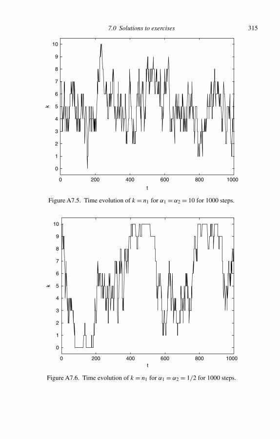
7.0 Solutions to exercises 315
0 200 400 600 800 1000
0
1
2
3
4
5
6
7
8
9
10
t
k
Figure A7.5. Time evolution of k = n1 for α1 = α2 = 10 for 1000 steps.
0 200 400 600 800 1000
0
1
2
3
4
5
6
7
8
9
10
t
k
Figure A7.6. Time evolution of k = n1 for α1 = α2 = 1/2 for 1000 steps.
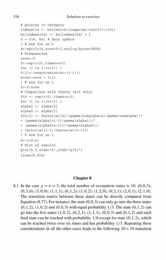
316 Solutions to exercises
# pointer to category
indexsite <- min(which((cumprobc-runif(1))>0))
bn[indexsite] <- bn[indexsite] + 1
A = c(A, bn) # data update
} # end for on t
A<-matrix(A,nrow=T+1,ncol=g,byrow=TRUE)
# Frequencies
norm<-0
f<-rep(c(0),times=n+1)
for (j in 1:(n+1)) {
f[j]<-length(which(A==(j-1)))
norm<-norm + f[j]
} # end for on j
f<-f/norm
# Comparison with theory (g=2 only)
fth <- rep(c(0),times=n+1)
for (i in 1:(n+1)) {
alpha1 <- alpha[2]
alpha0 <- alpha[1]
fth[i] <- factorial(n)/(gamma(sumalpha+n)/gamma(sumalpha))*
+ (gamma(alpha1+i-1)/gamma(alpha1))*
+ (gamma(alpha0+n-i+1)/gamma(alpha0))/
+ factorial(i-1)/factorial(n-i+1)
} # end for on i
k<-c(0:n)
# Plot of results
plot(k,f,xlab="k",ylab="p(k)")
lines(k,fth)
Chapter 8
8.1 In the case g = n = 3, the total number of occupation states is 10: (0,0,3);(0,3,0); (3,0,0); (1,1,1); (0,1,2); (1,0,2); (1,2,0); (0,2,1); (2,0,1); (2,1,0).The transition matrix between these states can be directly computed fromEquation (8.77). For instance, the state (0,0,3) can only go into the three states(0,1,2), (1,0,2) and (0,0,3) with equal probability 1/3. The state (0,1,2) cango into the five states (1,0,2), (0,2,1), (1,1,1), (0,0,3) and (0,1,2) and eachfinal state can be reached with probability 1/6 except for state (0,1,2), whichcan be reached twice over six times and has probability 1/3. Repeating theseconsiderations in all the other cases leads to the following 10 × 10 transition
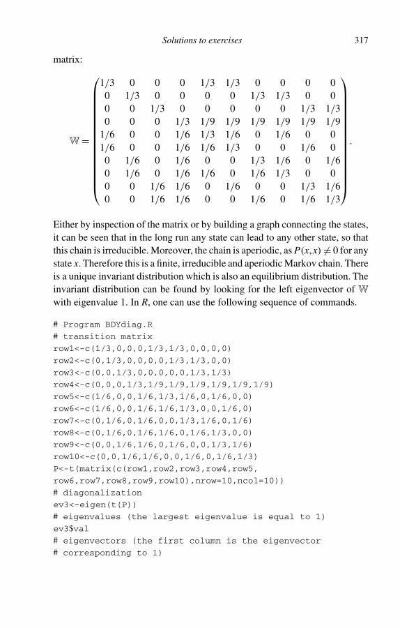
Solutions to exercises 317
matrix:
W =
1/3 0 0 0 1/3 1/3 0 0 0 00 1/3 0 0 0 0 1/3 1/3 0 00 0 1/3 0 0 0 0 0 1/3 1/30 0 0 1/3 1/9 1/9 1/9 1/9 1/9 1/9
1/6 0 0 1/6 1/3 1/6 0 1/6 0 01/6 0 0 1/6 1/6 1/3 0 0 1/6 00 1/6 0 1/6 0 0 1/3 1/6 0 1/60 1/6 0 1/6 1/6 0 1/6 1/3 0 00 0 1/6 1/6 0 1/6 0 0 1/3 1/60 0 1/6 1/6 0 0 1/6 0 1/6 1/3
.
Either by inspection of the matrix or by building a graph connecting the states,it can be seen that in the long run any state can lead to any other state, so thatthis chain is irreducible. Moreover, the chain is aperiodic, as P(x,x) �= 0 for anystate x. Therefore this is a finite, irreducible and aperiodic Markov chain. Thereis a unique invariant distribution which is also an equilibrium distribution. Theinvariant distribution can be found by looking for the left eigenvector of W
with eigenvalue 1. In R, one can use the following sequence of commands.
# Program BDYdiag.R
# transition matrix
row1<-c(1/3,0,0,0,1/3,1/3,0,0,0,0)
row2<-c(0,1/3,0,0,0,0,1/3,1/3,0,0)
row3<-c(0,0,1/3,0,0,0,0,0,1/3,1/3)
row4<-c(0,0,0,1/3,1/9,1/9,1/9,1/9,1/9,1/9)
row5<-c(1/6,0,0,1/6,1/3,1/6,0,1/6,0,0)
row6<-c(1/6,0,0,1/6,1/6,1/3,0,0,1/6,0)
row7<-c(0,1/6,0,1/6,0,0,1/3,1/6,0,1/6)
row8<-c(0,1/6,0,1/6,1/6,0,1/6,1/3,0,0)
row9<-c(0,0,1/6,1/6,0,1/6,0,0,1/3,1/6)
row10<-c(0,0,1/6,1/6,0,0,1/6,0,1/6,1/3)
P<-t(matrix(c(row1,row2,row3,row4,row5,
row6,row7,row8,row9,row10),nrow=10,ncol=10))
# diagonalization
ev3<-eigen(t(P))
# eigenvalues (the largest eigenvalue is equal to 1)
ev3$val# eigenvectors (the first column is the eigenvector
# corresponding to 1)
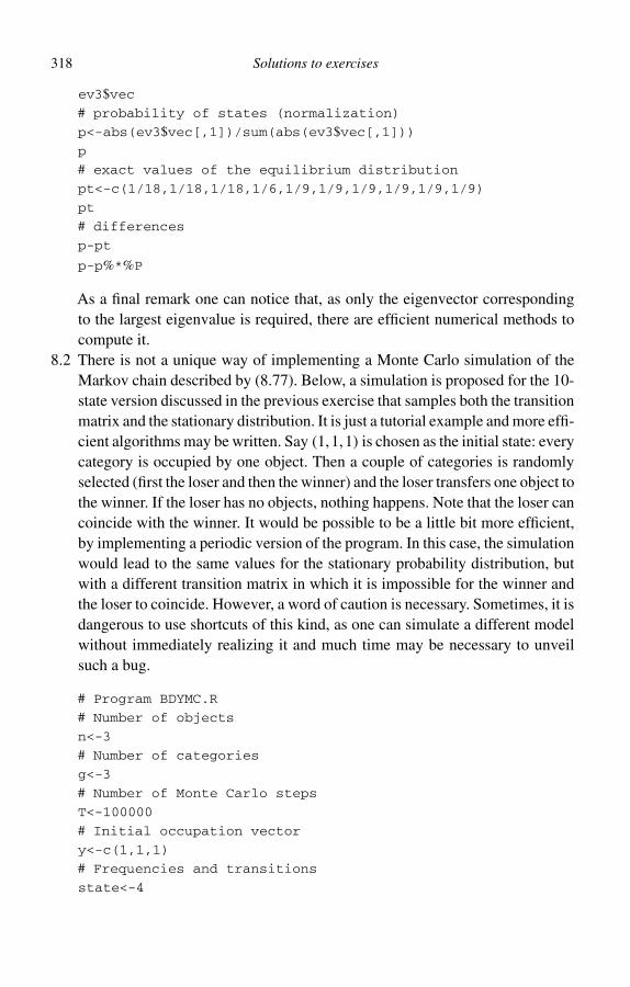
318 Solutions to exercises
ev3$vec# probability of states (normalization)
p<-abs(ev3$vec[,1])/sum(abs(ev3$vec[,1]))p
# exact values of the equilibrium distribution
pt<-c(1/18,1/18,1/18,1/6,1/9,1/9,1/9,1/9,1/9,1/9)
pt
# differences
p-pt
p-p%*%P
As a final remark one can notice that, as only the eigenvector correspondingto the largest eigenvalue is required, there are efficient numerical methods tocompute it.
8.2 There is not a unique way of implementing a Monte Carlo simulation of theMarkov chain described by (8.77). Below, a simulation is proposed for the 10-state version discussed in the previous exercise that samples both the transitionmatrix and the stationary distribution. It is just a tutorial example and more effi-cient algorithms may be written. Say (1,1,1) is chosen as the initial state: everycategory is occupied by one object. Then a couple of categories is randomlyselected (first the loser and then the winner) and the loser transfers one object tothe winner. If the loser has no objects, nothing happens. Note that the loser cancoincide with the winner. It would be possible to be a little bit more efficient,by implementing a periodic version of the program. In this case, the simulationwould lead to the same values for the stationary probability distribution, butwith a different transition matrix in which it is impossible for the winner andthe loser to coincide. However, a word of caution is necessary. Sometimes, it isdangerous to use shortcuts of this kind, as one can simulate a different modelwithout immediately realizing it and much time may be necessary to unveilsuch a bug.
# Program BDYMC.R
# Number of objects
n<-3
# Number of categories
g<-3
# Number of Monte Carlo steps
T<-100000
# Initial occupation vector
y<-c(1,1,1)
# Frequencies and transitions
state<-4
Solutions to exercises 319
freq<-c(0,0,0,0,0,0,0,0,0,0)
transmat<-matrix(0,nrow=10,ncol=10)
# Loop of Monte Carlo steps
for (i in 1:T) {# Random selection of the winner
# Generate a uniformly distributed integer between 1 and 3
indexw<-ceiling(3*runif(1))
# Random selection of the loser
# Generate a uniformly distributed integer between 1 and 3
indexl<-ceiling(3*runif(1))
# Verify if the loser has objects
while(y[indexl]==0) indexl<-ceiling(3*runif(1))
# Dynamic step
y[indexl]<-y[indexl]-1
y[indexw]<-y[indexw]+1
# frequencies
if (max(y)==1) newstate<-4
if (max(y)==3) {if(y[3]==3) newstate<-1
if(y[2]==3) newstate<-2
if(y[1]==3) newstate<-3
# end if
}if (max(y)==2) {if(y[1]==2) { if(y[2]==1) newstate<-10
else newstate<-9
# end if
}if(y[1]==1) { if(y[2]==2) newstate<-7
else newstate<-6
# end if
}if(y[1]==0) { if(y[2]==1) newstate<-5
else newstate<-8
# end if
}# end if
}# Updates
freq[newstate]<-freq[newstate]+1
transmat[newstate,state]<-transmat[newstate,state]+1
state<-newstate
# end for
}
320 Solutions to exercises
# Normalization
freq<-freq/T
freq
for (j in 1:10) transmat[j,]<-transmat[j,]/sum(transmat[j,])
transmat
# Differences
pt<-c(1/18,1/18,1/18,1/6,1/9,1/9,1/9,1/9,1/9,1/9)
pt-freq
row1<-c(1/3,0,0,0,1/3,1/3,0,0,0,0)
row2<-c(0,1/3,0,0,0,0,1/3,1/3,0,0)
row3<-c(0,0,1/3,0,0,0,0,0,1/3,1/3)
row4<-c(0,0,0,1/3,1/9,1/9,1/9,1/9,1/9,1/9)
row5<-c(1/6,0,0,1/6,1/3,1/6,0,1/6,0,0)
row6<-c(1/6,0,0,1/6,1/6,1/3,0,0,1/6,0)
row7<-c(0,1/6,0,1/6,0,0,1/3,1/6,0,1/6)
row8<-c(0,1/6,0,1/6,1/6,0,1/6,1/3,0,0)
row9<-c(0,0,1/6,1/6,0,1/6,0,0,1/3,1/6)
row10<-c(0,0,1/6,1/6,0,0,1/6,0,1/6,1/3)
P<-t(matrix(c(row1,row2,row3,row4,row5,
row6,row7,row8,row9,row10),nrow=10,ncol=10))
P-transmat
8.3 In Fig. A8.1, the Monte Carlo estimate of n∗i as the time average of the occu-
pation numbers ni(t) for T = 10000 Monte Carlo steps is compared to thetheoretical prediction given by Equation (8.62). This figure can be generatedby the following program.
# Program binary.R
# This program simulates the Ehrenfest-Brillouin model with
# binary moves and the constraint on energy (or demand).
# The energy (or demand) quantum is e = 1.
n <- 30 # number of particles
c <- 0 # c=1 for BE, c=0 for MB. (c = -1 for FD)
T <- 10000; # number of Monte Carlo steps
# We are only interested in the transitions
# between energy (or productivity) levels!
# Initial occupation vector. We start with all
# particles (workers) in a given cell of a given level.
# This fixes the energy (or production) of the system)
level <- 3
E <- level*n # total initial energy (production)
dmax <- E-(n-1) # the maximum level that can be occupied
q <- 0; # power for degeneracy of levels (0 for the original AYM)
i <- c(1:dmax) # number of levels
g <- iˆq; # degeneracy of levels
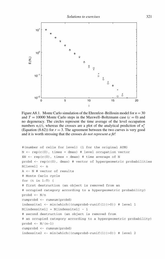
Solutions to exercises 321
0 5 10 15 2010−2
10−1
100
101
i
E(N
i)
Figure A8.1. Monte Carlo simulation of the Ehrenfest–Brillouin model for n = 30and T = 10000 Monte Carlo steps in the Maxwell–Boltzmann case (c = 0) andno degeneracy. The circles represent the time average of the level occupationnumbers ni(t), whereas the crosses are a plot of the analytical prediction of n∗
i(Equation (8.62)) for r = 3. The agreement between the two curves is very goodand it is worth stressing that the crosses do not represent a fit!
#(number of cells for level) (1 for the original AYM)
N <- rep(c(0), times = dmax) # level occupation vector
EN <- rep(c(0), times = dmax) # time average of N
probd <- rep(c(0), dmax) # vector of hypergeometric probabilities
N[level] <- n
A <- N # vector of results
# Monte Carlo cycle
for (t in 1:T) {
# first destruction (an object is removed from an
# occupied category according to a hypergeometric probability)
probd <- N/n
cumprobd <- cumsum(probd)
indexsite1 <- min(which((cumprobd-runif(1))>0)) # level 1
N[indexsite1] = N[indexsite1] - 1
# second destruction (an object is removed from
# an occupied category according to a hypergeometric probability)
probd <- N/(n-1)
cumprobd <- cumsum(probd)
indexsite2 <- min(which((cumprobd-runif(1))>0)) # level 2
322 Solutions to exercises
N[indexsite2] <- N[indexsite2] - 1
en <- indexsite1 + indexsite2 # energy (productivity) of the
# destroyed (removed) particles (workers)
en2 <- floor(en/2)
probc <- rep(c(0), times = en2) # probability of creation
# creation (the two particles reaccommodate
# according to a Polya probability)
for (j in 1:en2) {
probc[j] = 2*(g[j]+c*N[j])*(g[en-j]+c*N[en-j])
if (j==en-j) {
probc[j] <- probc[j]/2
} # end if
} # end for on j
cumprobc <- cumsum(probc/sum(probc))
indexsite3 <- min(which((cumprobc-runif(1))>0)) # level 3
N[indexsite3] <- N[indexsite3]+1
indexsite4 = en - indexsite3 # level 4
N[indexsite4] = N[indexsite4]+1
EN=EN+N/T # the average of N is stored
A = c(A, N); # data update
} # end for on t
A<-matrix(A,nrow=T+1,ncol=dmax,byrow=TRUE)
k=c(1:dmax)
plot(k,log(EN),xlab="i",ylab="N(i)")
ENth = (n*((level-1)/level)ˆk)/(level-1)
lines(k,log(ENth))

Author index
Aitchison J., 228Angle J., 228Aoki M., 217–219, 223, 227, 261Armatte M., 261
Bach A., 25Basharin G.P., 170Bennati E., 227Bergson A., 223Bernoulli D., 3Bernoulli J., 2, 3, 6, 32, 55Bernstein S.N., 170Bertrand J.L.F., 7, 8Billingsley P., 56, 57Boltzmann L., 19, 20, 25, 31, 39, 103, 105, 169,
218–220, 226, 227Bottazzi G., 203Brillouin L., 25, 39, 79–80, 94, 95, 172,
220, 226Brown J.A.C., 228
Caffè F., 223Carnap R., 12, 86, 124, 128, 129, 132Cauchy A.-L., 237Cavaliere G., 203Champernowne D.G., 228Church A., 41Costa M., 203Costantini D., 80, 94, 95, 124, 132, 203, 261Cowell F.A., 228Cox D.R., 288
Daboni L., 95de Finetti B., 2, 11, 12, 78, 86, 91, 245De Moivre A., 233Devlin K., 13Donnelly P., 261Doob J.L., 95Dosi G., 203Dragulescu A., 227Dubins L.E., 56, 57
Ehrenfest P., 31, 103, 139, 169, 172, 220, 226Ehrenfest T., 31, 103, 139, 169, 172, 220, 226Ewens W.J., 229, 236, 243, 245, 261
Fagiolo G., 203Feller W., 25Fermat P., 2, 13Fomin S.V., 94
Gardini A., 203Garibaldi U., 95, 203, 228, 261Gibbs J.W., 227Gibrat R., 261Gigerenzer G., 293Good I.J., 132Graberg D., 50
Hansen B., 261Hasenöhrl F., 25Hoel P.G., 170Hoppe F.M., 233, 261Hume D., 85Huygens C., 2, 10
Jacobs K., 95Jancel R., 203Jaynes E.T., xi, 8, 10, 12, 13, 123Jeffreys H., 12Johnson W.E., xii, 12, 86, 123, 124, 132
Kac M., 169, 170Karlin S., 95, 288Kemeny J.G., 170Kendall M.G., 25Keynes J.M., xii, 7, 12, 80, 86, 124Kirman A., 203Kolmogorov A.N., 9, 10, 12, 17, 35, 41, 46, 48,
54–56, 60, 73, 74, 87, 88, 91, 94
Laplace P.S., 3, 6, 8, 12, 32, 54, 56, 81, 83–85, 93,94, 296
323

324 Author index
Méré Chevalier de, 2Markov A.A., 169Maxwell J.C., 20, 31, 39, 226Merris R., 25Meyn S.P., 171Mill J.S., 66Miller H.D., 288Montmort P.-R., 68Mueser P.R., 50
Parzen E., 13Pascal B., 2, 13Pearson K., 124, 132Penco M.A., 203Pitman J., 261Pollard D., 56, 57Port S.C., 170
Ramsey F.P., 2, 11Rogers L.C.G., 288Ross S.M., 95
Savage L.J., 56, 57Scalas E., 228Schilling R.L., 56, 57Secchi A., 203Simon H., 265, 288
Sinai Ya.G., 25Snell J.L., 170Stegmüller W., 132Steindl J., 228Stone C.J., 170Stuart A., 25
Tavaré S., 236, 261Taylor H.M., 95, 288Tweedie R.L., 171
Viarengo P., 203, 261von Kries J., 7von Mises R., 9, 13, 41, 104
Wedlin A., 95Williams D., 288Willis J.C., 288Wio H., 169Wittgenstein L., 27
Yakovenko V.M., 227Yoshikawa H., 217–219, 223, 227Yule G.U., 288
Zabell S.L., 124, 132, 233, 256, 261
Subject index
σ -algebra, 56, 72n-exchangeable stochastic processes, 75, 76
Absorbing states for a Markov chain, 251–253, 272Aoki–Yoshikawa model for sectoral productivity,
217–219, 223, 227Aperiodic Markov chain, 146, 150, 152, 164
Bayes’ rule, 50Bayes’ theorem, 51Beta distribution, 92, 93, 283Beta–binomial distribution, 99Beta–Stacy distribution, 121Bienaymé–Chebyshev inequality, 159, 168Binomial distribution, 86, 99, 108, 109Binomial stochastic process, 106, 107Birth–death Markov chain, 139, 215Birth–death Simon–Zipf process, 269Birthday problem, 131Boolean algebra, 42, 55Boolean lattice
See Boolean algebra, 42Borel σ -algebra, 72Bravais–Pearson correlation coefficient, 66
Categorical random variables, 71Chapman–Kolmogorov equation, 142Chebyshev inequality, 159, 168Chinese restaurant process, 230Coefficient of variation, 101Complementary cumulative distribution
function, 60Conditional probability, 48Continuous random variables, 72Correlated random variables, 66Correlation, 65Countable additivity, 56, 72Countable random variables, 72Covariance, 58, 65, 66Cumulative distribution function, 60
De Morgan’s laws, 45Derangements, 70
Detailed balance, 134, 161, 162, 165, 166, 169, 172,175, 181, 196, 205, 248, 250, 254, 272, 307,308, 310
Diffusion process, 279Dirichlet distribution, 120Discrete random variables, 72Distance between probability distributions, 147Distribution
Beta, 92, 93, 283Beta–binomial, 99Beta–Stacy, 121Binomial, 86, 99, 108, 109Dirichlet, 120Gamma, 116, 117, 214Geometric, 104, 106, 107, 131Hypergeometric, 85, 86, 99, 109Joint, 65Leptokurtic, 193Log-normal, 224Log-series, 263Marginal, 65Marginalization of the Pólya, 104Mesokurtic, 193Multinomial, 108Negative binomial, 106–109, 116, 131, 190Normal, 192, 224Pólya, 96, 98, 283Pareto, 288Platykurtic, 193Poisson, 108, 109Uniform, 99Yule, 265, 288
Ehrenfest urn, 31, 103, 139, 143, 145, 147, 166, 167,169, 172, 220, 226
Ehrenfest–Brillouin model, x, 172, 180, 183, 194,201, 202, 203, 212, 214, 220, 222, 225, 226,231, 247, 260, 270, 283, 320
Equilibrium, statistical, x, xiii, 134, 139, 140, 146,152, 163, 164, 166, 168, 169, 175, 176, 178,179, 185–187, 189–191, 193, 197, 199–202,204, 212, 214–216, 218–220, 222, 223, 226,227, 232, 236, 244, 248–250, 252, 254, 257,
325
326 Subject index
263, 270, 271, 274, 275, 280, 287, 307,310, 312
Ergodic theorem for irreducible and aperiodicMarkov chains, 155
Ewens sampling formula, 229, 232Excess kurtosis, 190–192Exchangeable processes, 77Existence of the invariance distribution for
Markov chains, 153Expectation, 63Expected value, 58, 63, 93Expected value for the sum of m random
variables, 100
Falling factorial, 99Finite Markov chains, 134, 137, 139, 141, 149Finite random variable, 58, 60Finite stochastic process, 58, 73Fokker–Planck equation, 282Frequency spectrum, 243, 285Frequentism, 15Fundamental representation theorem for the Pólya
process, 123, 125Fundamental theorem of mathematical expectation, 64
Gamma distribution, 116, 117, 214Geometric distribution, 104, 106, 107, 131
Homogeneous Markov chain, 137, 139, 142Hoppe’s urn, 232–234, 256, 263Hypergeometric distribution, 85, 86, 99, 109Hypergeometric stochastic process, 75–78, 83, 85, 86,
90, 91
Image, 59Inclusion–exclusion formula, 68Independence of experiments, 53Independent events, 53Independent random variables, 66Indicator function, 67, 93Individual descriptions, Markov chain for, 165Invariant distribution for Markov chains, 150–153Inverse image, 59, 93Irreducible Markov chain, 144, 146, 150, 152, 164
Johnson’s sufficientness postulate, xii, 124, 125, 132Joint distribution, 65
Kolmogorov forward equation, 282Kolmogorov’s axioms for probability, 46Kolmogorov’s compatibility conditions, 74Kurtosis, 192
Label mixing, 104Lack of self-averaging, 225Lagrange multipliers, xi, 113, 131, 198, 206, 208, 219Laplace’s rule of succession, 83Law of large numbers for irreducible Markov
chains, 155Leptokurtic distribution, 193Log–normal distribution, 224Log–series distribution, 263
Logicism, 10Lower factorial
See falling factorial, 99
Map, 59Marginal distribution, 65Marginalization method, xiMarginalization of the Pólya distribution, 104Markov chain, 134, 137, 139, 141, 142, 149
Birth–death, 139, 215Existence of the invariant distribution, 150–152Limiting distributions, 150, 151Uniqueness of the invariant distribution, 150, 151
Markov chain for individual descriptions, 165Markov chains with a finite state space, 134, 137, 139,
141, 149Markov equation, 143Matching problem, 68Mathematical expectation, 63, 93Measurable functions, 59Measurable maps, 59Measurable space, 59Mesokurtic distribution, 193Metric space, 147Montmort’s matching problem, 68Monty Hall quiz, 49, 54Multinomial distribution, 108Multinomial stochastic process, 79Multiplication theorem, 49
Negative binomial distribution, 106–109, 116,131, 190
Neo-Bayesianism, 10Normal distribution, 192, 224Numerical random variables, 71
Pólya distribution, 96, 98, 283Pólya stochastic process, 79, 96Pólya stochastic process: fundamental representation
theorem, 123, 125Pareto distribution, 288Pauli’s exclusion principle, 78, 176Periodic Markov chain, 307Persistent states for a Markov chain, 144, 174,
175, 307Pigeonhole principle, 69Platykurtic distribution, 193Pochhammer symbol, 79, 98Poisson distribution, 108, 109Predictive law, 74Principle of indifference, 3, 8Principle of non-sufficient reason, 3Probability axioms, 46Probability, classical, 12Probability density function, 72Probability distribution, 60Probability of complement, 47Probability of empty set, 47Probability of the intersection of independent
events, 53Probability of union, 47
Subject index 327
Probability space, 46Product rule, 49Properties of indicator functions, 67, 93
Random variableCategorical, 71Continuous, 72Correlated, 66Countable, 72Discrete, 72Finite, 58, 60Independent, 66Numerical, 71Real, 72Relation between correlation and independence, 66Uncorrelated, 66
Random walkRandom walk with reflecting barriers, 139
Real random variables, 72Regular matrix, 150, 152, 153, 163, 167Retrodiction, 49Reversible Markov chain, 160, 162, 164Rising factorial, 79, 98, 237
Sampling stochastic processes, 74Self-averaging, 225Self-averaging sequence, 102Set function, 59Space
Measurable, 59Metric, 147
Standard deviation, 58, 65, 102, 110, 191Stationary Markov chain, 162, 164Statistical equilibrium, x, xiii, 134, 139, 140, 146,
152, 163, 164, 166, 168, 169, 175, 176, 178,179, 185–187, 189–191, 193, 197, 199–202,204, 212, 214–216, 218–220, 222, 223, 226,227, 232, 236, 244, 248–250, 252, 254, 257,263, 270, 271, 274, 275, 280, 287, 307, 310,312
Stirling’s approximation, 114, 198, 200, 219Stochastic matrix, 142, 148, 149, 173Stochastic process
n-Exchangeable, 75, 76Binomial, 106, 107Birth–death Simon–Zipf process, 269Chinese restaurant process, 230Definition in terms of a predictive law, 74Diffusion process, 279Exchangeable process, 77Finite, 58, 73Hypergeometric, 75–78, 83, 85, 86, 90, 91Multinomial, 79Pólya, 79, 96Sampling, 74
Subjectivism, 10Sufficientness postulate, 132
TheoremH -theorem, 220Theorem on reversible Markov chains, 162Bayes’ rule, 50Bayes’ theorem, 51Bernoulli, 3, 32de Finetti, 11, 245de Finetti representation theorem, finitary version,
78, 86, 91De Morgan’s laws, 45Ergodic theorem for irreducible and aperiodic
Markov chains, 155Expected value for the sum of m random
variables, 100Fundamental representation theorem for the Pólya
process, 123, 125Fundamental theorem of mathematical
expectation, 64Johnson’s representation theorem, 123Kolmogorov representation for stochastic
processes, 73Law of large numbers for irreducible Markov
chains, 155Multiplication theorem, 49Probability of complement, 47Probability of empty set, 47Probability of the intersection of independent
events, 53Probability of union, 47Product rule, 49Sinai’s theorem on irreducible and aperiodic
Markov chains, 150Theorem on positive stochastic matrices, 148Total probability, 50Variance of the sum of m random variables, 100
Total probability, 50Transient states for a Markov chain, 175, 252, 308Transition matrix, 142–146, 149–151, 162, 163, 165,
166, 168, 169, 184, 201, 225, 271, 280, 310,316, 317, 318
Transition probability, 137, 138, 140, 142, 153, 165,169, 172–174, 178, 184, 189, 194, 195, 201,204, 205, 212, 222, 225, 226, 231, 232, 248,250, 252, 280
Uncorrelated random variables, 66Uniform distribution, 99Unsigned Stirling numbers of the first kind, 238Upper factorial
See rising factorial, 79
Variance, 58, 64, 93Variance of the sum of m random variables, 100
Weak law of large numbers for irreducible Markovchains, 155
Yule distribution, 265, 288
Zipf’s urn, 262–264Zipf–Simon–Yule process, 262