Type Inference with Non-structural Subtyping∗

Jens Palsberg† Mitchell Wand‡§ Patrick O’Keefe¶

November 27, 2004

Abstract

We present an O(n3) time type inference algorithm for a typesystem with a largest type >, a smallest type⊥, and the usual orderingbetween function types. The algorithm infers type annotations ofleast shape, and it works equally well for recursive types. For theproblem of typability, our algorithm is simpler than the one of Kozen,Palsberg, and Schwartzbach for type inference without ⊥. This maybe surprising, especially because the system with ⊥ is strictly morepowerful.

∗Formal Aspects of Computing, 9:49–67, 1997.†Massachusetts Institute of Technology, NE43–340, 545 Technology Square, Cambridge,

MA 02139, USA. E-mail: palsberg@theory.lcs.mit.edu.‡Work supported by the National Science Foundation under grants CCR-9304144 and

CCR-9404646.§College of Computer Science, Northeastern University, 360 Huntington Avenue,

161CN, Boston, MA 02115, USA. E-mail: wand@ccs.neu.edu.¶151 Coolidge Avenue #211, Watertown, MA 02172, USA. E-mail:

pmo@world.std.com.

1

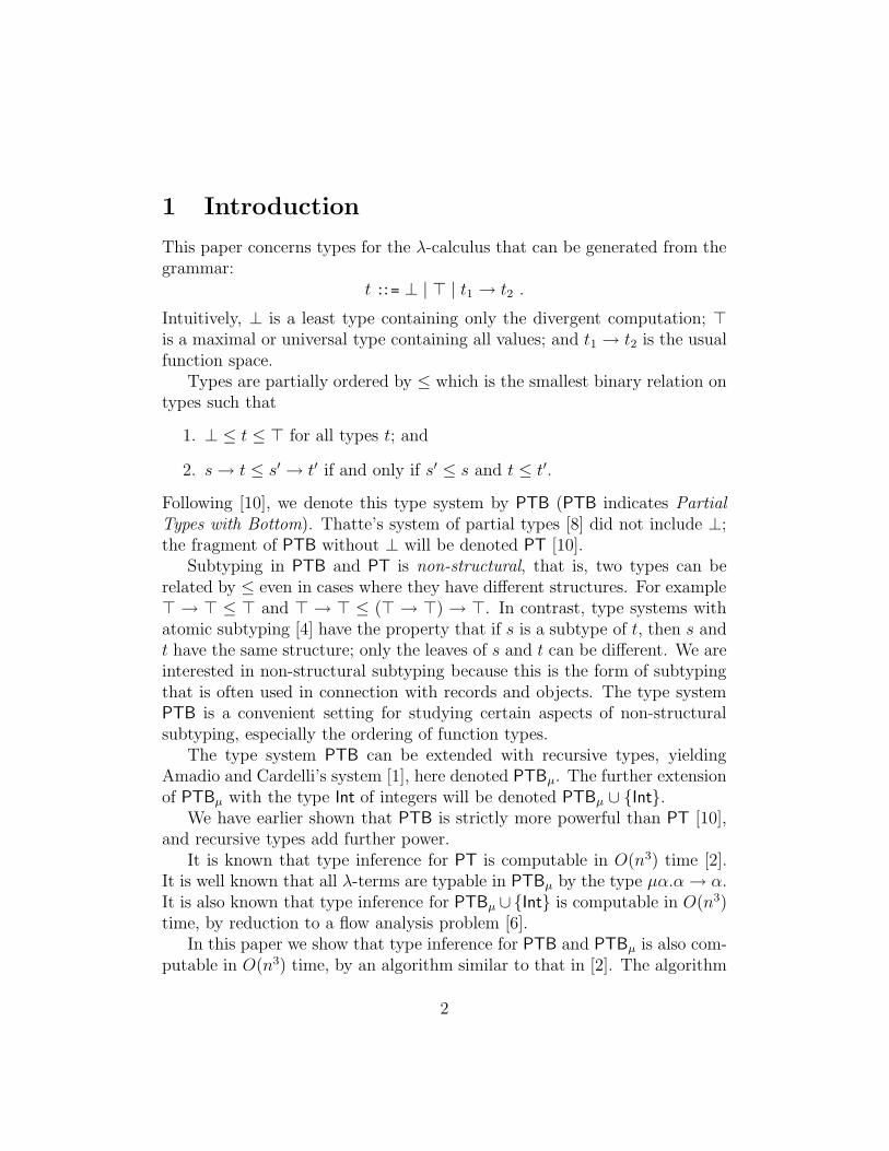
1 Introduction

This paper concerns types for the λ-calculus that can be generated from thegrammar:

t ::= ⊥ | > | t1 → t2 .

Intuitively, ⊥ is a least type containing only the divergent computation; >is a maximal or universal type containing all values; and t1 → t2 is the usualfunction space.

Types are partially ordered by ≤ which is the smallest binary relation ontypes such that

1. ⊥ ≤ t ≤ > for all types t; and

2. s→ t ≤ s′ → t′ if and only if s′ ≤ s and t ≤ t′.

Following [10], we denote this type system by PTB (PTB indicates Partial

Types with Bottom). Thatte’s system of partial types [8] did not include ⊥;the fragment of PTB without ⊥ will be denoted PT [10].

Subtyping in PTB and PT is non-structural, that is, two types can berelated by ≤ even in cases where they have different structures. For example> → > ≤ > and > → > ≤ (> → >) → >. In contrast, type systems withatomic subtyping [4] have the property that if s is a subtype of t, then s andt have the same structure; only the leaves of s and t can be different. We areinterested in non-structural subtyping because this is the form of subtypingthat is often used in connection with records and objects. The type systemPTB is a convenient setting for studying certain aspects of non-structuralsubtyping, especially the ordering of function types.

The type system PTB can be extended with recursive types, yieldingAmadio and Cardelli’s system [1], here denoted PTBµ. The further extensionof PTBµ with the type Int of integers will be denoted PTBµ ∪ {Int}.

We have earlier shown that PTB is strictly more powerful than PT [10],and recursive types add further power.

It is known that type inference for PT is computable in O(n3) time [2].It is well known that all λ-terms are typable in PTBµ by the type µα.α→ α.It is also known that type inference for PTBµ ∪{Int} is computable in O(n3)time, by reduction to a flow analysis problem [6].

In this paper we show that type inference for PTB and PTBµ is also com-putable in O(n3) time, by an algorithm similar to that in [2]. The algorithm

2

infers type annotations of least shape. A type is a tree (which can be infiniteif we consider recursive types), so its shape is the set of paths from the root.In general, there can be several types of least shape. For example, the λ-termλx.λy.(λf.f(fx))(λv.vy) can be typed such that

x : ⊥

y : ⊥

f : ⊥ → ⊥

v : ⊥ .

These type annotations are of least shape. If we replace the type of y by>, then we obtain another type annotation of least shape. The above λ-term and the two typings themselves are not particularly interesting, but itis the smallest example we have found for which there are more than oneleast-shape typing.

By contrast, in the type system PT, every typable λ-term has exactlyone type annotation of least shape. The algorithm by Kozen, Palsberg, andSchwartzbach [2] infers this least-shape type annotation.

The type inference algorithm by Palsberg and O’Keefe [6] for PTBµ∪{Int}does in general not infer type annotations of least shape. It remains open ifour result can be extended to PTBµ ∪ {Int}.

For the problem of typability, our algorithm is simpler than the one ofKozen, Palsberg, and Schwartzbach for type inference without ⊥. This maybe surprising, especially because the system with ⊥ is strictly more powerful.In our view, the simpler algorithm motivates having > and ⊥ together in atype system.

Our algorithm proceeds by first calculating a compact representation ofthe shape of a type for each subterm, and then assigning ⊥ or > to each leaf.Our method for choosing between ⊥ and > is simple and it seems possiblethat it can be generalized to work for richer type systems.

In the following section we define the type inference problem and summa-rize some known results that will be helpful in the later sections. In Section3 we define an automaton that will be used when defining possible solutionsto the type inference problem, and in Section 4 we define a useful notion ofupper bound. In Section 5 we prove our main theorem, which characterizesa least-shape solution, and in Section 6 we present our type inference algo-rithm. Finally, in Section 7 we give an example of how our type inference

3

algorithm works.

2 The type system

2.1 Type rules

If E is a λ-term, t is a type, and A is a type environment, i.e. a partialfunction assigning types to variables, then the judgement

A ` E : t

means that E has the type t in the environment A. Formally, this holdswhen the judgement is derivable using the following four rules:

A ` x : t (provided A(x) = t)

A[x← s] ` E : t

A ` λx.E : s→ t

A ` E : s→ t A ` F : s

A ` EF : t

A ` E : s s ≤ t

A ` E : t

The first three rules are the usual rules for simple types and the last rule isthe rule of subsumption.

The type system has the subject reduction property, that is, if A ` E : t isderivable and E β-reduces to E ′, then A ` E ′ : t is derivable. This is provedby straightforward induction on the structure of the derivation of A ` E : t[5].

This system types λ-terms which are not typable in the simply-typed λ-calculus. For example, consider λf.(fK(fI)), where K and I are the usualcombinators. This is not typable in the ordinary calculus, since K and I

have different types, but it is typable under partial typing: assign f the type> → (> → >). Both the K and I can be coerced to type >, and the result(fI), of type > → >, can be coerced to > to form the second argument ofthe first f . Therefore the entire λ-term has type (> → (> → >))→ >.

Similarly, some self-application is possible: (λx.xx) has type (> → t)→ t

for all t, since the final x can be coerced to >.

4

However, not all λ-terms are typable in this system. Any λ-term typablein PTB is strongly normalizing [10]. To indicate the flavor of those stronglynormalizing λ-terms which are not typable in this system, we have earlier[10] showed that (λx.xxx)(λy.y) is not typable in PTB. We also showed that(λf.f(fx))(λv.vy) is typable in PTB but not in PT. This demonstrates that⊥ adds power to a type system.

2.2 Constraints

Given a λ-term E, the type inference problem can be rephrased in terms ofsolving a system of type constraints. Assume that E has been α-convertedso that all bound variables are distinct. Let XE be the set of λ-variables xoccurring in E, and let YE be a set of variables disjoint from XE consistingof one variable [[F ]] for each occurrence of a subterm F of E. (The notation[[F ]] is ambiguous because there may be more than one occurrence of F inE. However, it will always be clear from context which occurrence is meant.)We generate the following system of inequalities over XE ∪ YE:

• for every occurrence in E of a subterm of the form λx.F , the inequality

x→ [[F ]] ≤ [[λx.F ]] ;

• for every occurrence in E of a subterm of the form GH, the inequality

[[G]] ≤ [[H]]→ [[GH]] ;

• for every occurrence in E of a λ-variable x, the inequality

x ≤ [[x]] .

Denote by T (E) the system of constraints generated from E in this fashion.For every λ-term E, let Tmap(E) be the set of total functions from XE ∪ YE

to the set of types. The function ψ ∈ Tmap(E) is a solution of T (E) if andonly if it is a solution of each constraint in T (E). Specifically, for V, V ′, V ′′ ∈XE ∪ YE:

The constraint: has solution ψ if:V → V ′ ≤ V ′′ ψ(V )→ ψ(V ′) ≤ ψ(V ′′)V ≤ V ′ → V ′′ ψ(V ) ≤ ψ(V ′)→ ψ(V ′′)

V ≤ V ′ ψ(V ) ≤ ψ(V ′)

5

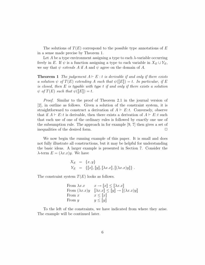
The solutions of T (E) correspond to the possible type annotations of Ein a sense made precise by Theorem 1.

Let A be a type environment assigning a type to each λ-variable occurringfreely in E. If ψ is a function assigning a type to each variable in XE ∪ YE,we say that ψ extends A if A and ψ agree on the domain of A.

Theorem 1 The judgement A ` E : t is derivable if and only if there exists

a solution ψ of T (E) extending A such that ψ([[E]]) = t. In particular, if E

is closed, then E is typable with type t if and only if there exists a solution

ψ of T (E) such that ψ([[E]]) = t.

Proof. Similar to the proof of Theorem 2.1 in the journal version of[2], in outline as follows. Given a solution of the constraint system, it isstraightforward to construct a derivation of A ` E: t. Conversely, observethat if A ` E: t is derivable, then there exists a derivation of A ` E: t suchthat each use of one of the ordinary rules is followed by exactly one use ofthe subsumption rule. The approach in for example [9, 7] then gives a set ofinequalities of the desired form. 2

We now begin the running example of this paper. It is small and doesnot fully illustrate all constructions, but it may be helpful for understandingthe basic ideas. A larger example is presented in Section 7. Consider theλ-term E = (λx.x)y. We have

XE = {x, y}

YE = {[[x]], [[y]], [[λx.x]], [[(λx.x)y]]} .

The constraint system T (E) looks as follows.

From λx.x x→ [[x]] ≤ [[λx.x]]From (λx.x)y [[λx.x]] ≤ [[y]]→ [[(λx.x)y]]From x x ≤ [[x]]From y y ≤ [[y]]

To the left of the constraints, we have indicated from where they arise.The example will be continued later.

6

2.3 A representation of types

We will use a standard representation of types that will be convenient inSections 3–6. Intuitively, a type is a binary tree where its interior nodes arelabeled with → and its leaves are labeled with > or ⊥. A path from the rootof a type can be thought of as a string of 0’s and 1’s. Starting at the root,as long as the nodes along the path are labeled with an arrow, a 0 in thepath selects the left subtree, a 1 selects the right subtree. In the followingwe formalize this intuition, along the lines of for example [3, 6].

Let Σ = {→,⊥,>} be the ranked alphabet where → is binary and ⊥,>are nullary. A type is a finite tree over Σ. A path from the root of such a treeis a string over {0, 1}, where 0 indicates “left subtree” and 1 indicates “rightsubtree”. This set of types is the same as the one defined by the grammarin Section 1. A set S of strings is prefix closed if αβ ∈ S implies α ∈ S. Werepresent a type by a term, which is a function mapping each path from theroot of the type to the symbol at the end of the path, as follows.

Definition 2 A term is a partial function

t : {0, 1}∗ → Σ

with domain D(t) such that D(t) is non-empty and prefix-closed, and suchthat if t(α) =→, then {i | αi ∈ D(t)} = {0, 1}; and if t(α) ∈ {⊥,>}, then{i | αi ∈ D(t)} = ∅. The set of all such terms is denoted TΣ. The setof terms with finite domain is denoted FΣ. They represent finite trees, byKonig’s Lemma. In our application, FΣ is the set of types.

For s, t ∈ TΣ, define→TΣ: TΣ×TΣ → TΣ and ⊥TΣ ,>TΣ ∈ TΣ with domains

D(s→TΣ t) = {ε} ∪ {0α | α ∈ D(s)} ∪ {1α | α ∈ D(t)}

D(⊥TΣ) = {ε}

D(>TΣ) = {ε}

by

(s→TΣ t)(0α) = s(α)

(s→TΣ t)(1α) = t(α)

(s→TΣ t)(ε) = →

⊥TΣ(ε) = ⊥

>TΣ(ε) = > .

7

For t ∈ TΣ and α ∈ {0, 1}∗, define the partial function t↓α : {0, 1}∗ → Σ by

t↓α(β) = t(αβ) .

If t ↓α has non-empty domain, then it is a term, and is called the subtermof t at position α.

For x ⊆ {0, 1}∗ and α ∈ {0, 1}∗, define x ↓ α = {β | αβ ∈ x}. Noticethat the notation ↓ is overloaded. Which definition is being used will beclear from context. 2

The following properties are immediate from the definitions:

(i) (s→TΣ t)↓0 = s

(ii) (s→TΣ t)↓1 = t

(iii) (t↓α)↓β = t↓αβ

Following [3], we henceforth omit the superscript TΣ on the operators→TΣ, ⊥TΣ , >TΣ .

We will say that a term s has smaller shape than a term t if D(s) ⊆ D(t).Our type inference algorithm will infer types that are of least shape.

Terms are ordered by the subtype relation ≤, as follows.

Definition 3 The parity of α ∈ {0, 1}∗ is the number mod 2 of 0’s in α.The parity of α is denoted πα. A string α is said to be even if πα = 0 andodd if πα = 1. Let ≤0 be the partial order on Σ given by

⊥ ≤0 → and → ≤0 >

and let ≤1 be its reverse

> ≤1 → and → ≤1 ⊥ .

For s, t ∈ TΣ, define s ≤ t if s(α) ≤πα t(α) for all α ∈ D(s) ∩ D(t). 2

Kozen, Palsberg, and Schwartzbach [3] showed that the relation ≤ isequivalent to the order defined by Amadio and Cardelli [1]. The relation ≤is a partial order with ⊥ ≤ t ≤ > for all t ∈ TΣ, and s → t ≤ s′ → t′ if andonly if s′ ≤ s and t ≤ t′ [1, 3]. Moreover, on FΣ, ≤ coincides with the typeordering defined in Section 1 [3].

8

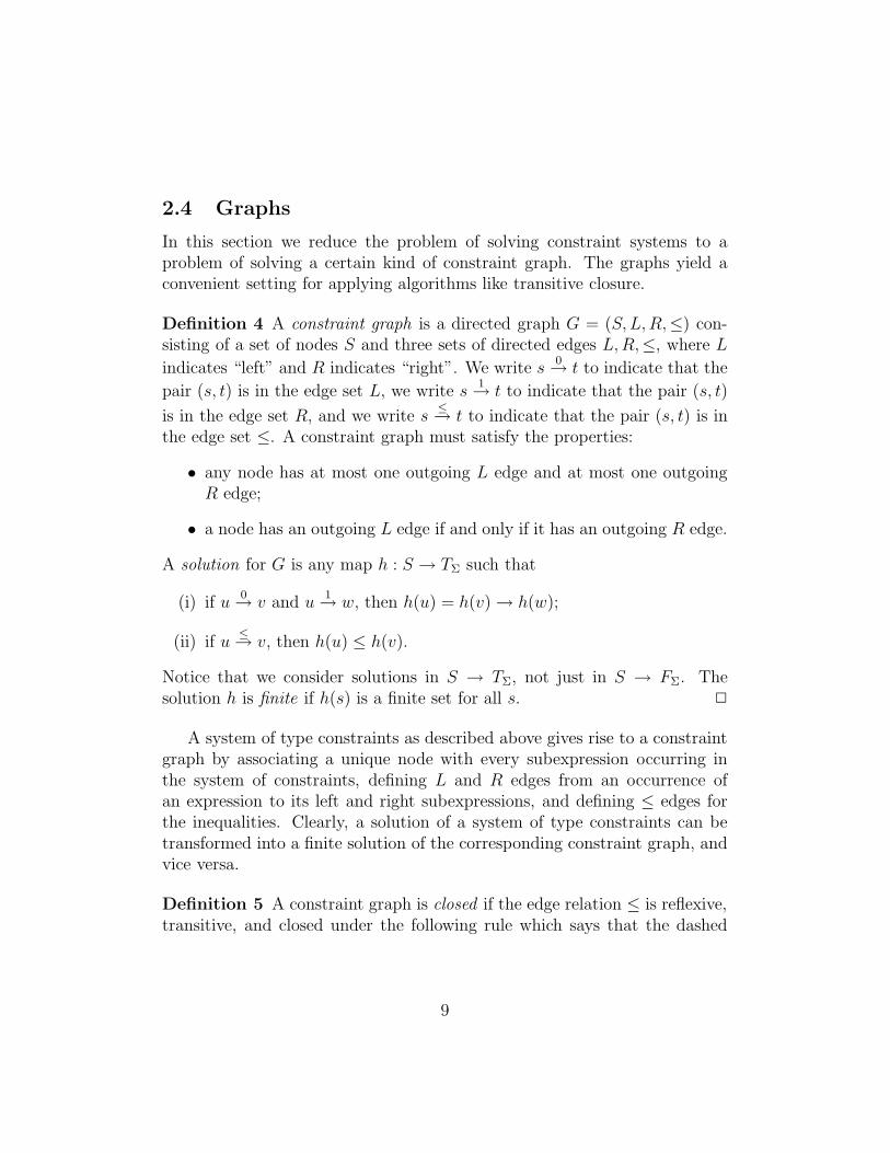
2.4 Graphs

In this section we reduce the problem of solving constraint systems to aproblem of solving a certain kind of constraint graph. The graphs yield aconvenient setting for applying algorithms like transitive closure.

Definition 4 A constraint graph is a directed graph G = (S, L,R,≤) con-sisting of a set of nodes S and three sets of directed edges L,R,≤, where L

indicates “left” and R indicates “right”. We write s0→ t to indicate that the

pair (s, t) is in the edge set L, we write s1→ t to indicate that the pair (s, t)

is in the edge set R, and we write s≤→ t to indicate that the pair (s, t) is in

the edge set ≤. A constraint graph must satisfy the properties:

• any node has at most one outgoing L edge and at most one outgoingR edge;

• a node has an outgoing L edge if and only if it has an outgoing R edge.

A solution for G is any map h : S → TΣ such that

(i) if u0→ v and u

1→ w, then h(u) = h(v)→ h(w);

(ii) if u≤→ v, then h(u) ≤ h(v).

Notice that we consider solutions in S → TΣ, not just in S → FΣ. Thesolution h is finite if h(s) is a finite set for all s. 2

A system of type constraints as described above gives rise to a constraintgraph by associating a unique node with every subexpression occurring inthe system of constraints, defining L and R edges from an occurrence ofan expression to its left and right subexpressions, and defining ≤ edges forthe inequalities. Clearly, a solution of a system of type constraints can betransformed into a finite solution of the corresponding constraint graph, andvice versa.

Definition 5 A constraint graph is closed if the edge relation ≤ is reflexive,transitive, and closed under the following rule which says that the dashed

9

edges exist whenever the solid ones do:

�-

-BBBBBN

��

��

���

BBBBBN

��

��

���≥

≤

≤

1010

The closure of a constraint graph G is the smallest closed graph containingG as a subgraph. 2

Lemma 6 A constraint graph and its closure have the same set of solutions.

Proof. Any solution of the closure of G is also a solution of G, since Ghas fewer constraints. Conversely, the closure of G can be constructed fromG by iterating the closure rules, and it follows inductively that any solutionof G satisfies the additional constraints added by this process. 2

Consider again the running example E = (λx.x)y. We use the followingabbreviations

The symbol: abbreviates:→1 x→ [[x]]→2 [[y]]→ [[(λx.x)y]]

The constraint graph generated from T (E) looks as follows.

- -

-

��

����

AAAAAU

AAAAAU

��

����

6

→1 →2

≤ ≤

≤

≤

[[λx.x]]

0 1 0 1

x [[x]] [[y]] [[(λx.x)y]]

y

10

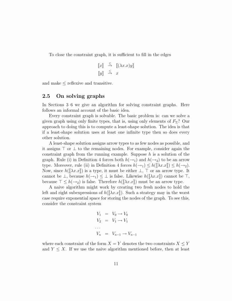
To close the constraint graph, it is sufficient to fill in the edges

[[x]]≤→ [[(λx.x)y]]

[[y]]≤→ x

and make ≤ reflexive and transitive.

2.5 On solving graphs

In Sections 3–6 we give an algorithm for solving constraint graphs. Herefollows an informal account of the basic idea.

Every constraint graph is solvable. The basic problem is: can we solve agiven graph using only finite types, that is, using only elements of FΣ? Ourapproach to doing this is to compute a least-shape solution. The idea is thatif a least-shape solution uses at least one infinite type then so does everyother solution.

A least-shape solution assigns arrow types to as few nodes as possible, andit assigns > or ⊥ to the remaining nodes. For example, consider again theconstraint graph from the running example. Suppose h is a solution of thegraph. Rule (i) in Definition 4 forces both h(→1) and h(→2) to be an arrowtype. Moreover, rule (ii) in Definition 4 forces h(→1) ≤ h([[λx.x]]) ≤ h(→2).Now, since h([[λx.x]]) is a type, it must be either ⊥, > or an arrow type. Itcannot be ⊥, because h(→1) ≤ ⊥ is false. Likewise h([[λx.x]]) cannot be >,because > ≤ h(→2) is false. Therefore h([[λx.x]]) must be an arrow type.

A naive algorithm might work by creating two fresh nodes to hold theleft and right subexpressions of h([[λx.x]]). Such a strategy may in the worstcase require exponential space for storing the nodes of the graph. To see this,consider the constraint system

V1 = V0 → V0

V2 = V1 → V1

. . .

Vn = Vn−1 → Vn−1

where each constraint of the form X = Y denotes the two constraints X ≤ Y

and Y ≤ X. If we use the naive algorithm mentioned before, then at least

11

2n nodes will be generated. Moreover, care needs to be taken to ensure thatthe naive algorithm terminates in cases where an infinite type is required.

To sidestep these problems we shift the focus from the question

“which nodes have to be assigned an arrow type?”

to the question

“what set of paths have to be in the type for a given node?”

The first question is easy to answer, but it has to be repeated and answeredmany times before a solution is constructed. The second question seems moredifficult, but it turns out that we can encode the necessary paths using timeand space which is polynomial in the size of the graph. The basic idea is touse a nondeterministic automaton, as shown in the following section.

3 An automaton

We now present the key construction (Definition 7) that we will use to effi-ciently solve constraint graphs. Given a closed constraint graph, the idea isto construct an automaton that

• keeps track of upper and lower bounds in the graph, and

• accepts paths that must exist in every solution of the graph.

In the following sections we will use the automaton to construct a solution ofleast shape. Each state in the automaton is a pair of nodes from the graph.Moreover, we ensure that if a state (u′, v′) is reachable from a state of the

form (u, u), then u′≤→ v′ is in the graph (Lemma 8). The language accepted

by the automaton is a set of paths. If s is a node in the constraint graph andwe take (s, s) as the start state of the automaton, then the accepted pathsmust be in the domain of every type for s (Lemma 9). The present sectionincludes three useful results (Lemmas 10, 11, 12) about the automaton; theywill be applied in later sections.

Definition 7 Let a constraint graph G = (S, L,R,≤) be given. The au-tomaton M is defined as follows. The input alphabet of M is {0, 1}. The

12

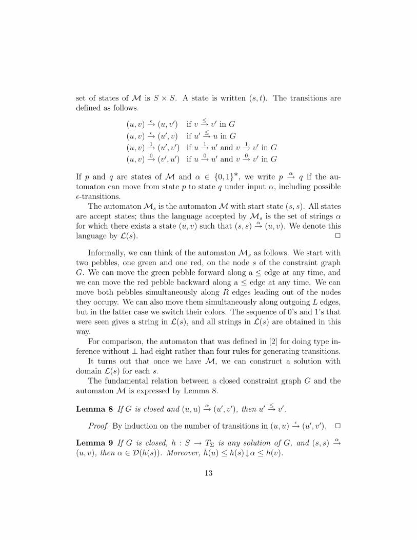
set of states of M is S × S. A state is written (s, t). The transitions aredefined as follows.

(u, v)ε→ (u, v′) if v

≤→ v′ in G

(u, v)ε→ (u′, v) if u′

≤→ u in G

(u, v)1→ (u′, v′) if u

1→ u′ and v

1→ v′ in G

(u, v)0→ (v′, u′) if u

0→ u′ and v

0→ v′ in G

If p and q are states of M and α ∈ {0, 1}∗, we write pα→ q if the au-

tomaton can move from state p to state q under input α, including possibleε-transitions.

The automatonMs is the automatonM with start state (s, s). All statesare accept states; thus the language accepted by Ms is the set of strings αfor which there exists a state (u, v) such that (s, s)

α→ (u, v). We denote this

language by L(s). 2

Informally, we can think of the automatonMs as follows. We start withtwo pebbles, one green and one red, on the node s of the constraint graphG. We can move the green pebble forward along a ≤ edge at any time, andwe can move the red pebble backward along a ≤ edge at any time. We canmove both pebbles simultaneously along R edges leading out of the nodesthey occupy. We can also move them simultaneously along outgoing L edges,but in the latter case we switch their colors. The sequence of 0’s and 1’s thatwere seen gives a string in L(s), and all strings in L(s) are obtained in thisway.

For comparison, the automaton that was defined in [2] for doing type in-ference without ⊥ had eight rather than four rules for generating transitions.

It turns out that once we have M, we can construct a solution withdomain L(s) for each s.

The fundamental relation between a closed constraint graph G and theautomatonM is expressed by Lemma 8.

Lemma 8 If G is closed and (u, u)α→ (u′, v′), then u′

≤→ v′.

Proof. By induction on the number of transitions in (u, u)ε→ (u′, v′). 2

Lemma 9 If G is closed, h : S → TΣ is any solution of G, and (s, s)α→

(u, v), then α ∈ D(h(s)). Moreover, h(u) ≤ h(s)↓α ≤ h(v).

13

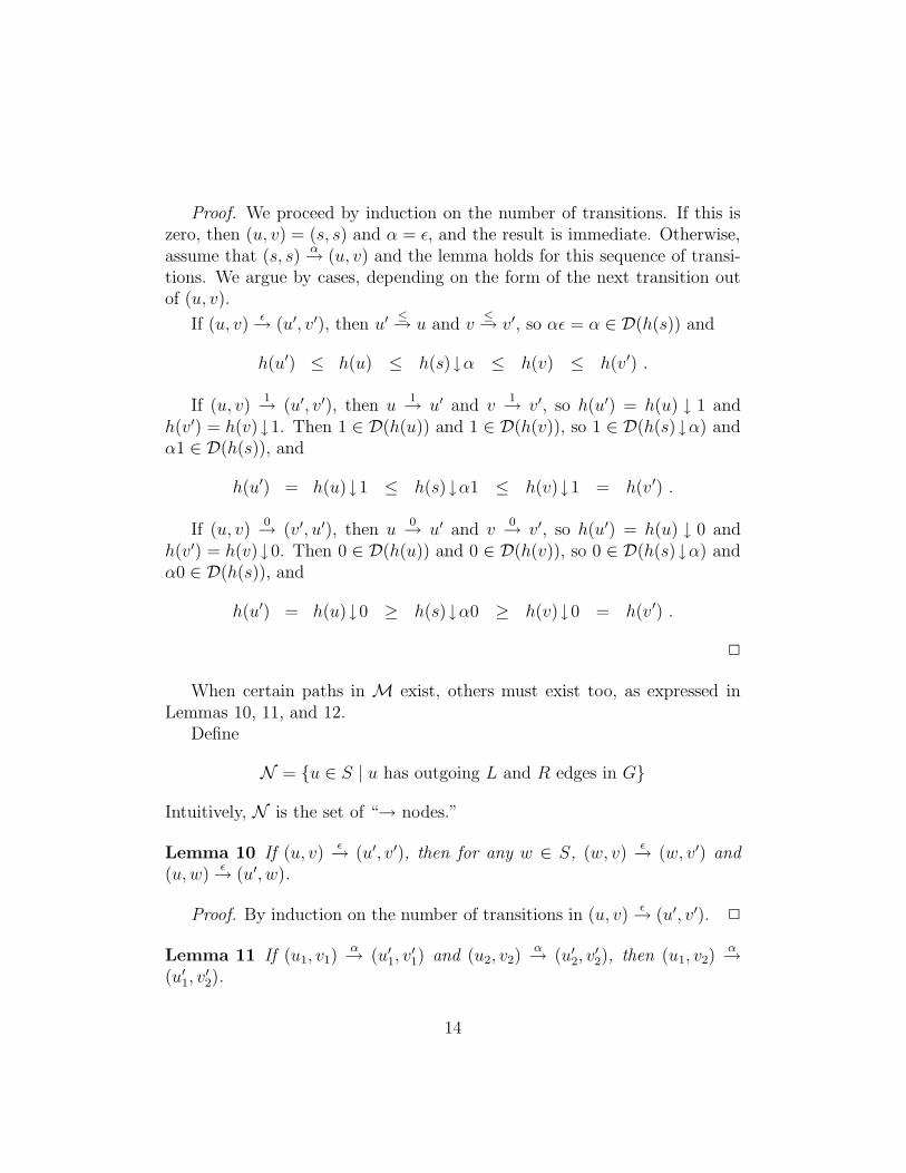
Proof. We proceed by induction on the number of transitions. If this iszero, then (u, v) = (s, s) and α = ε, and the result is immediate. Otherwise,assume that (s, s)

α→ (u, v) and the lemma holds for this sequence of transi-

tions. We argue by cases, depending on the form of the next transition outof (u, v).

If (u, v)ε→ (u′, v′), then u′

≤→ u and v

≤→ v′, so αε = α ∈ D(h(s)) and

h(u′) ≤ h(u) ≤ h(s)↓α ≤ h(v) ≤ h(v′) .

If (u, v)1→ (u′, v′), then u

1→ u′ and v

1→ v′, so h(u′) = h(u) ↓ 1 and

h(v′) = h(v)↓1. Then 1 ∈ D(h(u)) and 1 ∈ D(h(v)), so 1 ∈ D(h(s)↓α) andα1 ∈ D(h(s)), and

h(u′) = h(u)↓1 ≤ h(s)↓α1 ≤ h(v)↓1 = h(v′) .

If (u, v)0→ (v′, u′), then u

0→ u′ and v

0→ v′, so h(u′) = h(u) ↓ 0 and

h(v′) = h(v)↓0. Then 0 ∈ D(h(u)) and 0 ∈ D(h(v)), so 0 ∈ D(h(s)↓α) andα0 ∈ D(h(s)), and

h(u′) = h(u)↓0 ≥ h(s)↓α0 ≥ h(v)↓0 = h(v′) .

2

When certain paths in M exist, others must exist too, as expressed inLemmas 10, 11, and 12.

Define

N = {u ∈ S | u has outgoing L and R edges in G}

Intuitively, N is the set of “→ nodes.”

Lemma 10 If (u, v)ε→ (u′, v′), then for any w ∈ S, (w, v)

ε→ (w, v′) and

(u, w)ε→ (u′, w).

Proof. By induction on the number of transitions in (u, v)ε→ (u′, v′). 2

Lemma 11 If (u1, v1)α→ (u′

1, v′

1) and (u2, v2)

α→ (u′

2, v′

2), then (u1, v2)

α→

(u′1, v′

2).

14

Proof. We proceed by induction on the length of α. In the base case,consider α with length 0. We then have α = ε, so by Lemma 10,

(u1, v2)ε→ (u′

1, v2)

ε→ (u′

1, v′

2) .

In the induction step, consider first

(u1, v1)α1→ (u′

1, v′

1)

(u2, v2)α1→ (u′

2, v′

2) .

In both cases, let us make explicit the 1-transition, that is, find x1, y1, x2, y2 ∈N and x′

1, y′

1, x′

2, y′

2∈ S such that

(u1, v1)α→ (x1, y1)

1→ (x′

1, y′

1)

ε→ (u′

1, v′

1)

(u2, v2)α→ (x2, y2)

1→ (x′

2, y′

2)

ε→ (u′

2, v′

2)

and x1

1→ x′

1, y1

1→ y′

1, x2

1→ x′

2, y2

1→ y′

2. From the induction hypothesis

and Lemma 10 we get

(u1, v2)α→ (x1, y2)

1→ (x′

1, y′

2)

ε→ (u′

1, y′

2)

ε→ (u′

1, v′

2) .

Consider then

(u1, v1)α0→ (u′

1, v′

1)

(u2, v2)α0→ (u′

2, v′

2) .

Again, let us make explicit the 0-transition, that is, find x1, y1, x2, y2 ∈ Nand x′

1, y′

1, x′

2, y′

2∈ S such that

(u1, v1)α→ (x1, y1)

0→ (y′

1, x′

1)

ε→ (u′

1, v′

1)

(u2, v2)α→ (x2, y2)

0→ (y′

2, x′

2)

ε→ (u′

2, v′

2)

and x1

0→ x′

1, y1

0→ y′

1, x2

0→ x′

2, y2

0→ y′

2. From the induction hypothesis

and Lemma 10 we get

(u1, v2)α→ (x2, y1)

0→ (y′

1, x′

2)

ε→ (u′

1, x′

2)

ε→ (u′

1, v′

2) .

2

15

Lemma 12 Suppose i ∈ {0, 1}, ui→ v, and α ∈ L(v). If G is closed, then

L(v)↓α = L(u)↓ iα.

Proof. Clearly, L(v)↓α ⊆ L(u)↓ iα. To prove the converse, suppose

(u, u)i→ (u1, v1)

α→ (x, y)

β→ (x′, y′) .

From (u, u)i→ (v, v) and Lemma 11 we get

(u, u)i→ (u1, v)

(u, u)i→ (v, v1) .

From Lemma 8 we get u1

≤→ v

≤→ v1, hence

(v, v)ε→ (u1, v1)

α→ (x, y)

β→ (x′, y′) ,

so L(v)↓α ⊇ L(u)↓ iα. 2

Consider again the running example E = (λx.x)y. The constraint graphgenerated from T (E) has 8 nodes, so the automaton M has 82 = 64 states.The following picture shows some of the states reachable from the state([[λx.x]], [[λx.x]]).

-�

ZZ

ZZ

ZZ~

��

��

��=

��

��

��=

ZZ

ZZ

ZZ~

(→1, [[λx.x]]) ([[λx.x]],→2)

(→1,→2)

([[y]], x) ([[x]], [[(λx.x)y]])

([[λx.x]], [[λx.x]])

0 1

ε ε

ε ε

It turns out that L(x) = L(y) = {ε} and L([[λx.x]]) = {ε, 0, 1}.

16

4 Upper bounds

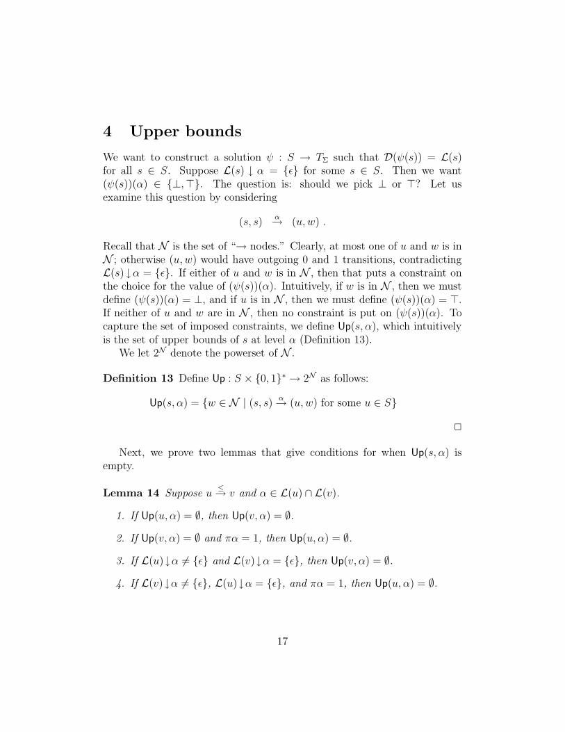
We want to construct a solution ψ : S → TΣ such that D(ψ(s)) = L(s)for all s ∈ S. Suppose L(s) ↓ α = {ε} for some s ∈ S. Then we want(ψ(s))(α) ∈ {⊥,>}. The question is: should we pick ⊥ or >? Let usexamine this question by considering

(s, s)α→ (u, w) .

Recall that N is the set of “→ nodes.” Clearly, at most one of u and w is inN ; otherwise (u, w) would have outgoing 0 and 1 transitions, contradictingL(s)↓α = {ε}. If either of u and w is in N , then that puts a constraint onthe choice for the value of (ψ(s))(α). Intuitively, if w is in N , then we mustdefine (ψ(s))(α) = ⊥, and if u is in N , then we must define (ψ(s))(α) = >.If neither of u and w are in N , then no constraint is put on (ψ(s))(α). Tocapture the set of imposed constraints, we define Up(s, α), which intuitivelyis the set of upper bounds of s at level α (Definition 13).

We let 2N denote the powerset of N .

Definition 13 Define Up : S × {0, 1}∗ → 2N as follows:

Up(s, α) = {w ∈ N | (s, s)α→ (u, w) for some u ∈ S}

2

Next, we prove two lemmas that give conditions for when Up(s, α) isempty.

Lemma 14 Suppose u≤→ v and α ∈ L(u) ∩ L(v).

1. If Up(u, α) = ∅, then Up(v, α) = ∅.

2. If Up(v, α) = ∅ and πα = 1, then Up(u, α) = ∅.

3. If L(u)↓α 6= {ε} and L(v)↓α = {ε}, then Up(v, α) = ∅.

4. If L(v)↓α 6= {ε}, L(u)↓α = {ε}, and πα = 1, then Up(u, α) = ∅.

17

Proof. To prove (1), suppose Up(v, α) 6= ∅. Choose w ∈ N and u′ ∈ Ssuch that (v, v)

α→ (u′, w). Choose also u1, v1 ∈ S such that (u, u)

α→ (u1, v1).

From u≤→ v and Lemma 11 we then get

(u, u)ε→ (u, v)

α→ (u1, w) ,

contradicting Up(u, α) = ∅.To prove (2), suppose Up(u, α) 6= ∅. Since πα = 1, we can write α = β0γ

where β ∈ {0, 1}∗ and γ ∈ {1}∗. Choose x1, y1, w ∈ N and x2, y2, u′ ∈ S

such that

(u, u)β→ (x1, y1)

0→ (y2, x2)

γ→ (u′, w)

and x1

0→ x2 and y1

0→ y2. Choose p1, q1 ∈ N and p2, q2, u

′′, v′′ ∈ S such that

(v, v)β→ (p1, q1)

0→ (q2, p2)

γ→ (u′′, v′′)

and p1

0→ p2 and q1

0→ q2. From u

≤→ v and Lemma 11 we then get

(v, v)ε→ (u, v)

β→ (x1, q1)

0→ (q2, x2)

γ→ (u′′, w) ,

contradicting Up(v, α) = ∅.To prove (3), suppose Up(v, α) 6= ∅. Choose w ∈ N and u′ ∈ S such

that (v, v)α→ (u′, w). Choose also x, y ∈ N such that (u, u)

α→ (x, y). From

u≤→ v and Lemma 11 we get

(v, v)ε→ (u, v)

α→ (x, w) ,

contradicting L(v)↓α = {ε}.To prove (4), suppose Up(u, α) 6= ∅. Since πα = 1, we can write α = β0γ

where β ∈ {0, 1}∗ and γ ∈ {1}∗. Choose x1, y1, w ∈ N and x2, y2, u′ ∈ S

such that

(u, u)β→ (x1, y1)

0→ (y2, x2)

γ→ (u′, w)

and x1

0→ x2 and y1

0→ y2. Since L(v) ↓ α 6= {ε}, choose p1, q1, u

′′, v′′ ∈ Nand p2, q2 ∈ S such that

(v, v)β→ (p1, q1)

0→ (q2, p2)

γ→ (u′′, v′′)

18

and p1

0→ p2 and q1

0→ q2. From u

≤→ v and Lemma 11 we then get

(u, u)ε→ (u, v)

β→ (x1, q1)

0→ (q2, x2)

γ→ (u′′, w) ,

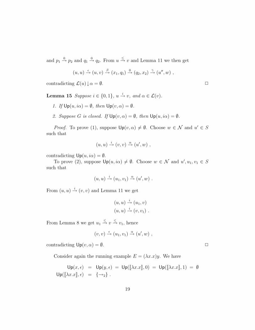
contradicting L(u)↓α = ∅. 2

Lemma 15 Suppose i ∈ {0, 1}, ui→ v, and α ∈ L(v).

1. If Up(u, iα) = ∅, then Up(v, α) = ∅.

2. Suppose G is closed. If Up(v, α) = ∅, then Up(u, iα) = ∅.

Proof. To prove (1), suppose Up(v, α) 6= ∅. Choose w ∈ N and u′ ∈ Ssuch that

(u, u)i→ (v, v)

α→ (u′, w) ,

contradicting Up(u, iα) = ∅.To prove (2), suppose Up(u, iα) 6= ∅. Choose w ∈ N and u′, u1, v1 ∈ S

such that

(u, u)i→ (u1, v1)

α→ (u′, w) .

From (u, u)i→ (v, v) and Lemma 11 we get

(u, u)i→ (u1, v)

(u, u)i→ (v, v1) .

From Lemma 8 we get u1

≤→ v

≤→ v1, hence

(v, v)ε→ (u1, v1)

α→ (u′, w) ,

contradicting Up(v, α) = ∅. 2

Consider again the running example E = (λx.x)y. We have

Up(x, ε) = Up(y, ε) = Up([[λx.x]], 0) = Up([[λx.x]], 1) = ∅

Up([[λx.x]], ε) = {→2} .

19

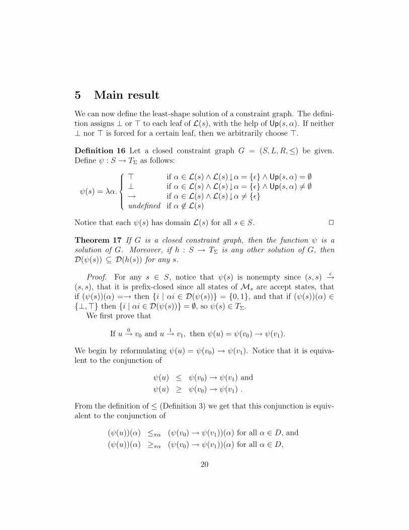
5 Main result

We can now define the least-shape solution of a constraint graph. The defini-tion assigns ⊥ or > to each leaf of L(s), with the help of Up(s, α). If neither⊥ nor > is forced for a certain leaf, then we arbitrarily choose >.

Definition 16 Let a closed constraint graph G = (S, L,R,≤) be given.Define ψ : S → TΣ as follows:

ψ(s) = λα.

> if α ∈ L(s) ∧ L(s)↓α = {ε} ∧ Up(s, α) = ∅⊥ if α ∈ L(s) ∧ L(s)↓α = {ε} ∧ Up(s, α) 6= ∅→ if α ∈ L(s) ∧ L(s)↓α 6= {ε}undefined if α 6∈ L(s)

Notice that each ψ(s) has domain L(s) for all s ∈ S. 2

Theorem 17 If G is a closed constraint graph, then the function ψ is a

solution of G. Moreover, if h : S → TΣ is any other solution of G, then

D(ψ(s)) ⊆ D(h(s)) for any s.

Proof. For any s ∈ S, notice that ψ(s) is nonempty since (s, s)ε→

(s, s), that it is prefix-closed since all states of Ms are accept states, thatif (ψ(s))(α) =→ then {i | αi ∈ D(ψ(s))} = {0, 1}, and that if (ψ(s))(α) ∈{⊥,>} then {i | αi ∈ D(ψ(s))} = ∅, so ψ(s) ∈ TΣ.

We first prove that

If u0→ v0 and u

1→ v1, then ψ(u) = ψ(v0)→ ψ(v1).

We begin by reformulating ψ(u) = ψ(v0) → ψ(v1). Notice that it is equiva-lent to the conjunction of

ψ(u) ≤ ψ(v0)→ ψ(v1) and

ψ(u) ≥ ψ(v0)→ ψ(v1) .

From the definition of ≤ (Definition 3) we get that this conjunction is equiv-alent to the conjunction of

(ψ(u))(α) ≤πα (ψ(v0)→ ψ(v1))(α) for all α ∈ D, and

(ψ(u))(α) ≥πα (ψ(v0)→ ψ(v1))(α) for all α ∈ D,

20

where D = D(ψ(u)) ∩ D(ψ(v0) → ψ(v1)). Since ≤πα is a partial order, wecan fold the second conjunction into the single condition

(ψ(u))(α) = (ψ(v0)→ ψ(v1))(α) for all α ∈ D.

To prove that u0→ v0 and u

1→ v1 implies this condition, notice first that

(ψ(u))(ε) = (ψ(v0)→ ψ(v1))(ε) =→. Then, let i ∈ {0, 1} and iα ∈ D(ψ(u))∩D(ψ(v0)→ ψ(v1)). It is sufficient to prove

(ψ(u))(iα) = (ψ(vi))(α) .

There are three cases. Suppose (ψ(vi))(α) =→. Then L(vi) ↓ α 6= {ε}.From Lemma 12 we get L(u) ↓ iα 6= {ε}, so (ψ(u))(iα) =→. Supposethen (ψ(vi))(α) = ⊥. Then L(vi) ↓ α = {ε} and Up(vi, α) 6= ∅. FromLemma 15.1 we get Up(u, iα) 6= ∅. From Lemma 12 we get L(u)↓ iα = {ε},so (ψ(u))(iα) = ⊥. Suppose finally (ψ(vi))(α) = >. Then L(vi) ↓ α = {ε}and Up(vi, α) = ∅. From Lemma 15.2 we get Up(u, iα) = ∅. From Lemma 12we get L(u)↓ iα = {ε}, so (ψ(u))(iα) = >.

We then prove that

If u≤→ v, then ψ(u) ≤ ψ(v).

Suppose α ∈ D(ψ(u)) ∩ D(ψ(v)) = L(u) ∩ L(v). We then need to prove(ψ(u))(α) ≤πα (ψ(v))(α). There are two cases.

Suppose first πα = 0. If (ψ(u))(α) = ⊥, then the result is immediate.If (ψ(u))(α) = >, then L(u) ↓α = {ε} and Up(u, α) = ∅. By Lemma 14.1,Up(v, α) = ∅. Hence, L(v) ↓ α = {ε}, so (ψ(v))(α) = >, from which theresult follows. If (ψ(u))(α) =→, then there are two cases. If L(v)↓α 6= {ε},then (ψ(v))(α) =→, from which the result follows. If L(v) ↓α = {ε}, thenit follows from Lemma 14.3 that Up(v, α) = ∅. Hence, (ψ(v))(α) = >, fromwhich the result follows.

Suppose then πα = 1. If (ψ(v))(α) = ⊥, then the result is immediate.If (ψ(v))(α) = >, then L(v) ↓ α = {ε} and Up(v, α) = ∅. By Lemma 14.2,Up(u, α) = ∅. Hence, L(u) ↓ α = {ε}, so (ψ(u))(α) = >, from which theresult follows. If (ψ(v))(α) =→, then there are two cases. If L(u)↓α 6= {ε},then (ψ(u))(α) =→, from which the result follows. If L(u) ↓α = {ε}, thenit follows from Lemma 14.4 that Up(u, α) = ∅. Hence, (ψ(u))(α) = >, fromwhich the result follows.

21

To show that ψ is a solution of least shape, we need to show that for anyother solution h : S → TΣ of G, D(ψ(s)) ⊆ D(h(s)) for any s. This followsdirectly from Lemma 9. 2

Consider for the last time the running example E = (λx.x)y. We get

ψ(x) = ψ([[x]]) = ψ(y) = ψ([[y]]) = ψ([[(λx.x)y]]) = >

ψ([[λx.x]]) = > → > .

6 An Algorithm

We have shown that the type inference problem for PTB can be reduced tosolving constraint graphs. Using the characterization of Theorem 17, we geta straightforward type inference algorithm.

Theorem 18 One can decide in time O(n3) whether a constraint graph of

size n has a finite solution.

Proof. By Theorem 17, there exists a finite solution if and only if theconstructed solution ψ has the property that ψ(s) is finite for all s ∈ D(ψ)).To determine this, we need only check whether any L(s) contains an infinitepath. We first form the constraint graph, then close it; this gives a graphwith n vertices and O(n2) edges. This can be done in time O(n3). We thenform the automaton M, which has n2 states but only O(n3) transitions, atmost O(n) from each state. We then check for a cycle with at least one non-εtransition reachable from some (s, s). This can be done in linear time in thesize of the graph using depth-first search. The entire algorithm requires timeO(n3). 2

A λ-term of size n yields a constraint graph with O(n) nodes and O(n)edges. Allowing types to be represented succinctly by the automataMs, weget our main result.

Corollary 19 The type inference problem for PTB is solvable in O(n3) time.

Recursive types are just regular trees [1]. The least-shape solution wehave constructed, although possibly infinite, is a regular tree for every nodein the constraint graph. Thus, we get the following result.

22

Corollary 20 For PTBµ, we can infer a least-shape type annotation in O(n3)time.

It remains open how to extend this result to PTBµ ∪ {Int}.

7 Example

We now give an example of how our type inference algorithm works. Considerthe λ-term E = (λx.xx)(λy.y) which was also treated in [6]. We give eachof the two occurrences of x a label so that the λ-term reads (λx.x1x2)(λy.y).The constraint system T (E) looks as follows:

From λx.x1x2 x→ [[x1x2]] ≤ [[λx.x1x2]]From λy.y y → [[y]] ≤ [[λy.y]]From E [[λx.x1x2]] ≤ [[λy.y]]→ [[E]]From x1x2 [[x1]] ≤ [[x2]]→ [[x1x2]]From x1 x ≤ [[x1]]From x2 x ≤ [[x2]]From y y ≤ [[y]]

To the left of the constraints, we have indicated from where they arise.We will use the following abbreviations:

The symbol: abbreviates:→1 x→ [[x1x2]]→2 y → [[y]]→3 [[λy.y]]→ [[E]]→4 [[x2]]→ [[x1x2]]

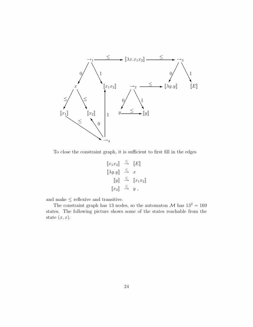
The constraint graph derived from T (E) looks as follows:

23

- -

��

��

���

AAAAAAU

��

��

��

AAAAAU

��

��

��

AAAAAU

6 AAAAAU

��

��

��

QQ

QQ

QQ

QQQs

JJ

JJJ]

-

-

→1

→2

→3

→4

[[λx.x1x2]]

[[x1x2]] [[λy.y]] [[E]]

[[x1]] [[y]][[x2]]

x

y

≤

≤ ≤

≤ ≤

≤

≤

00

0

0

1 1

1

1

To close the constraint graph, it is sufficient to first fill in the edges

[[x1x2]]≤→ [[E]]

[[λy.y]]≤→ x

[[y]]≤→ [[x1x2]]

[[x2]]≤→ y ,

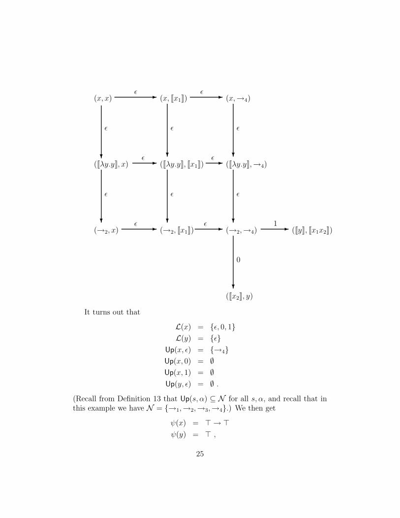
and make ≤ reflexive and transitive.The constraint graph has 13 nodes, so the automaton M has 132 = 169

states. The following picture shows some of the states reachable from thestate (x, x).

24

- -

- -

- - -

?

?

? ?

? ?

?

(x, x) (x, [[x1]]) (x,→4)

([[λy.y]], x) ([[λy.y]], [[x1]]) ([[λy.y]],→4)

(→2, x) (→2, [[x1]]) (→2,→4) ([[y]], [[x1x2]])

([[x2]], y)

ε

ε ε

ε ε

ε ε ε

ε ε

ε ε 1

0

It turns out that

L(x) = {ε, 0, 1}

L(y) = {ε}

Up(x, ε) = {→4}

Up(x, 0) = ∅

Up(x, 1) = ∅

Up(y, ε) = ∅ .

(Recall from Definition 13 that Up(s, α) ⊆ N for all s, α, and recall that inthis example we have N = {→1,→2,→3,→4}.) We then get

ψ(x) = > → >

ψ(y) = > ,

25

and it turns out that E is typable.For comparison, we can apply the algorithm of [6] for type inference for

PTB extended with recursive types to E. The result is that both x and y getannotated by the infinite type µα.α→ α [6].

References

[1] Roberto M. Amadio and Luca Cardelli. Subtyping recursive types. ACM

Transactions on Programming Languages and Systems, 15(4):575–631,1993. Also in Proc. POPL’91.

[2] Dexter Kozen, Jens Palsberg, and Michael I. Schwartzbach. Efficientinference of partial types. Journal of Computer and System Sciences,49(2):306–324, 1994. Preliminary version in Proc. FOCS’92, 33rd IEEESymposium on Foundations of Computer Science, pages 363–371, Pitts-burgh, Pennsylvania, October 1992.

[3] Dexter Kozen, Jens Palsberg, and Michael I. Schwartzbach. Efficientrecursive subtyping. Mathematical Structures in Computer Science,5(1):113–125, 1995. Preliminary version in Proc. POPL’93, TwentiethAnnual SIGPLAN–SIGACT Symposium on Principles of ProgrammingLanguages, pages 419–428, Charleston, South Carolina, January 1993.

[4] John Mitchell. Coercion and type inference. In Eleventh Symposium on

Principles of Programming Languages, pages 175–185, 1984.

[5] John C. Mitchell. Type inference with simple subtypes. Journal of

Functional Programming, 1:245–285, 1991.

[6] Jens Palsberg and Patrick M. O’Keefe. A type system equivalent to flowanalysis. ACM Transactions on Programming Languages and Systems,17(4):576–599, July 1995. Preliminary version in Proc. POPL’95, 22ndAnnual SIGPLAN–SIGACT Symposium on Principles of ProgrammingLanguages, pages 367–378, San Francisco, California, January 1995.

[7] Jens Palsberg and Michael I. Schwartzbach. Safety analysis versus typeinference for partial types. Information Processing Letters, 43:175–180,1992.

26

[8] Satish Thatte. Type inference with partial types. In Proc. Interna-

tional Colloquium on Automata, Languages, and Programming 1988,pages 615–629. Springer-Verlag (LNCS 317), 1988.

[9] Mitchell Wand. Type inference for record concatenation and multipleinheritance. Information and Computation, 93(1):1–15, 1991.

[10] Mitchell Wand, Patrick M. O’Keefe, and Jens Palsberg. Strong nor-malization with non-structural subtyping. Mathematical Structures in

Computer Science, 5(3):419–430, 1995.

27