Two-Parameter Rayleigh Distribution: Different

Methods of Estimation

Sanku Dey∗, Tanujit Dey†, and Debasis Kundu‡

∗Department of Statistics, St. Anthony’s College, Shillong, Meghalaya, India. Email:

sanku dey2k2003@yahoo.co.in†Department of Mathematics, Jones Hall, The College of William & Mary, Williamsburg, Virginia, USA.

Email: tdey@wm.edu‡Department of Mathematics and Statistics, Indian Institute of Technology, Kanpur, India. Email:

kundu@iitk.ac.in

1

2

Abstract

In this paper we have considered different methods of estimation of the unknown

parameters of a two-parameter Rayleigh distribution both from the frequentists and

Bayesian view points. First we briefly describe different frequentists approaches, namely

maximum likelihood estimators, moments estimators, L-moment estimators, percentile

based estimators and least squares estimators, and compare them using extensive nu-

merical simulations. We have also considered Bayesian inferences of the unknown pa-

rameters. It is observed that the Bayes estimates and the associated credible intervals

cannot be obtained in explicit forms, and we have suggested to use importance sam-

pling technique to compute the Bayes estimates and the associated credible intervals.

We analyze one data set for illustrative purposes.

Key Words and Phrases: Maximum likelihood estimators; method of moment estimators;

L-moment estimators; least squares estimators; weighted least squares estimators; percentile

based estimators; Bayes estimators, asymptotic distribution; simulation consistent estima-

tors.

3

1 Introduction

Lord Rayleigh (1880) introduced the Rayleigh distribution in connection with a problem in

the field of acoustics. Since then, extensive work has taken place related to this distribution

in different areas of science and technology. It has some nice relations with some of the well

known distributions like Weibull, chi-square or extreme value distributions. An important

characteristic of the Rayleigh distribution is that its hazard function is an increasing function

of time. It means that when the failure times are distributed according to the Rayleigh

law, an intense aging of the equipment/ item takes place. Estimations, predictions and

inferential issues for one parameter Rayleigh distribution have been extensively studied by

several authors. Interested readers may have a look at the book by Johnson, Kotz and

Balakrishnan (1994) for an excellent exposure of the Rayleigh distribution, and see also

Abd-Elfattah, Hassan and Ziedean (2006), Dey and Das (2007), Dey (2009) for some recent

references.

In this paper we consider two-parameter Rayleigh distribution; one scale and one location

parameter, and it has the following probability density function (PDF)

f(x;λ, µ) = 2λ(x− µ)e−λ(x−µ)2 ; x > µ, λ > 0. (1)

The corresponding cumulative distribution function (CDF) for x > µ, is as follows;

F (x;λ, µ) = 1− e−λ(x−µ)2 . (2)

Here λ and µ are the scale and location parameters respectively. Interestingly, although ex-

tensive work has been done on one-parameter Rayleigh distribution, not much attention has

been paid to two-parameter Rayleigh distribution, although Johnson, Kotz and Balakrish-

nan (1994) briefly mentioned about the two-parameter Rayleigh distribution in their book.

Recently, Khan, Provost and Singh (2010) considered two-parameter Rayleigh distribution

and discussed some inferential issues.

4

The main aim of this paper is to consider different estimation procedures of the two-

parameter Rayleigh distribution both from the Bayesian and frequentist points of view. We

first consider the most natural frequentist’s estimators namely the maximum likelihood esti-

mators (MLEs). The MLEs of the two-parameter Rayleigh distribution cannot be obtained

in explicit forms. They can be obtained by solving a one dimensional optimization process.

We have provided a very simple iterative technique which can be used to compute the MLEs

of the unknown parameters. The two-parameter Rayleigh distribution does not satisfy the

standard regularity conditions of Cramer. In fact, some elements of the expected Fisher in-

formation matrix are not finite. Therefore, the standard asymptotic normality results of the

maximum likelihood estimators do not hold here. We provide the asymptotic distribution

of the MLEs, based on the results of Smith (1995).

Although, the MLEs do not have explicit forms, the method of moment estimators

(MMEs) can be obtained in explicit forms. We provide the MMEs and study their asymp-

totic properties. We also consider other estimators, namely least squares estimators, weighted

least squares estimators, percentile estimators and L-moment estimators. We further con-

sider the Bayes estimators of the unknown parameters under the assumptions of independent

gamma and uniform priors on the scale and shape parameters respectively. It is observed

that the Bayes estimators under the squared error loss function cannot be obtained in closed

forms. We have suggested use of importance sampling procedure to compute simulation con-

sistent Bayes estimate and the associated credible interval. We compare the performances

of the different methods using extensive computer simulations. Finally, we analyze a data

set for illustrative purposes.

Rest of the paper is organized as follows. In Section 2, we provide the MLEs of the

unknown parameters and discuss their asymptotic properties. The MMEs and their asymp-

totic properties are presented in Section 3. Percentile estimators and least squares estimators

5

are provided in Section 4 and Section 5 respectively. L-moment estimators are provided in

Section 6. Bayes estimators are presented in Section 7. In Section 8 we present the Monte

Carlo simulation results. The analysis of a real data set is provided in Section 9, and finally

conclusions appear in Section 10.

2 Maximum Likelihood Estimators

Let x1, · · · , xn be a random sample of size n from (1), then the log-likelihood function l(µ, λ)

without the additive constant for µ < x(1) = min{x1, · · · , xn} can be written as

l(µ, λ) = C + n lnλ+n∑

i=1

ln(xi − µ)− λn∑

i=1

(xi − µ)2. (3)

The two normal equations become

∂

∂λl(µ, λ) =

n

λ−

n∑

i=1

(xi − µ)2 = 0 (4)

∂

∂µl(µ, λ) = −

n∑

i=1

(xi − µ)−1 + 2λn∑

i=1

(xi − µ) = 0. (5)

From (4), we obtain the MLE of λ as a function of µ, say λ̂(µ), as

λ̂(µ) =n∑n

i=1(xi − µ)2. (6)

Substituting λ̂(µ) in (3), we obtain the profile log-likelihood function of µ without the addi-

tive constant as

g(µ) = −n ln(n∑

i=1

(xi − µ)2) +n∑

i=1

ln(xi − µ) =n∑

i=1

ln

[(xi − µ)∑ni=1(xi − µ)2

]. (7)

Therefore, the MLE of µ, say µ̂MLE, can be obtained by maximizing (7) with respect to µ.

It can be shown that the maximum of (7) can be obtained as a fixed point solution of the

following equation

h(µ) = µ, (8)

6

where

h(µ) = 2n∑

i=1

(xi − µ)2 ×n∑

i=1

(xi − µ)×n∑

i=1

(xi − µ)−1. (9)

Once µ̂MLE is obtained, the MLE of λ, λ̂MLE = λ̂(µ̂MLE) can be easily obtained. Observe

that very simple iterative technique namely h(µ(j)) = µ(j+1), where µ(j) is the j − th iterate,

can be used to solve (8).

Now we want to study the variances and distributional properties of µ̂MLE and λ̂MLE.

Since they are not in explicit forms, it is expected that the exact distributions of the MLEs

will not be possible to obtain. We therefore, mainly rely on the asymptotic properties of the

MLEs. The two-parameter Rayleigh distribution does not satisfy the standard regularity

conditions of Cramer. Note that

E

(∂2

∂µ2l(µ, λ)

)= 2nλ+ E

(n∑

i=1

(Xi − µ)2

)= ∞. (10)

From Theorem 3 of Smith (1985) it follows that (µ̂MLE − µ) is asymptotically normally

distributed with mean 0 and V (µ̂MLE −µ) = O

(1

n lnn

), and (λ̂MLE −λ) is asymptotically

normally distributed with mean 0 and V (λ̂MLE − λ) = −[E

(∂2l

∂λ2

)]−1

=λ2

n. Moreover, µ̂

and λ̂ are asymptotically independent. Although, the exact asymptotic variance of µ̂ cannot

be obtained in explicit form, from Corollary of Theorem 3 of Smith (1985), it follows that

V (µ̂− µ) can be well approximated by the inverse of the observed information, and in this

case it is

V (µ̂MLE − µ) ≈ 1

2µ+ 1n

∑ni=1(xi − µ)−2

. (11)

Therefore, 100(1− α)% approximate confidence intervals of λ and µ can be obtained as

λ̂MLE ± zα/2λ̂MLE√

nand µ̂MLE ± zα/2

(1

2µ̂MLE + 1n

∑ni=1(xi − µ̂MLE)−2

)1/2

, (12)

respectively, where zα/2 is the α/2-th percentile point of the standard normal distribution.

7

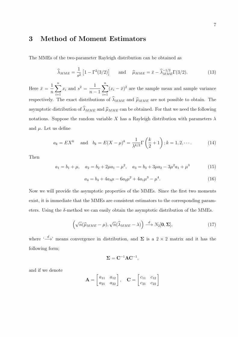
3 Method of Moment Estimators

The MMEs of the two-parameter Rayleigh distribution can be obtained as

λ̂MME =1

s2[1− Γ2(3/2)

]and µ̂MME = x̄− λ̂

−1/2MMEΓ(3/2). (13)

Here x̄ =1

n

n∑

i=1

xi and s2 =1

n− 1

n∑

i=1

(xi − x̄)2 are the sample mean and sample variance

respectively. The exact distributions of λ̂MME and µ̂MME are not possible to obtain. The

asymptotic distribution of λ̂MME and µ̂MME can be obtained. For that we need the following

notations. Suppose the random variable X has a Rayleigh distribution with parameters λ

and µ. Let us define

ak = EXk and bk = E(X − µ)k =1

λk/2Γ

(k

2+ 1

); k = 1, 2, · · · . (14)

Then

a1 = b1 + µ, a2 = b2 + 2µa1 − µ2, a3 = b3 + 3µa2 − 3µ2a1 + µ3 (15)

a4 = b4 + 4a3µ− 6a2µ2 + 4a1µ

3 − µ4. (16)

Now we will provide the asymptotic properties of the MMEs. Since the first two moments

exist, it is immediate that the MMEs are consistent estimators to the corresponding param-

eters. Using the δ-method we can easily obtain the asymptotic distribution of the MMEs.

(√n(µ̂MME − µ),

√n(λ̂MME − λ)

)d−→ N2[0,Σ], (17)

where ‘d−→’ means convergence in distribution, and Σ is a 2 × 2 matrix and it has the

following form;

Σ = C−1AC−1,

and if we denote

A =

[a11 a12a21 a22

], C =

[c11 c12c21 c22

]

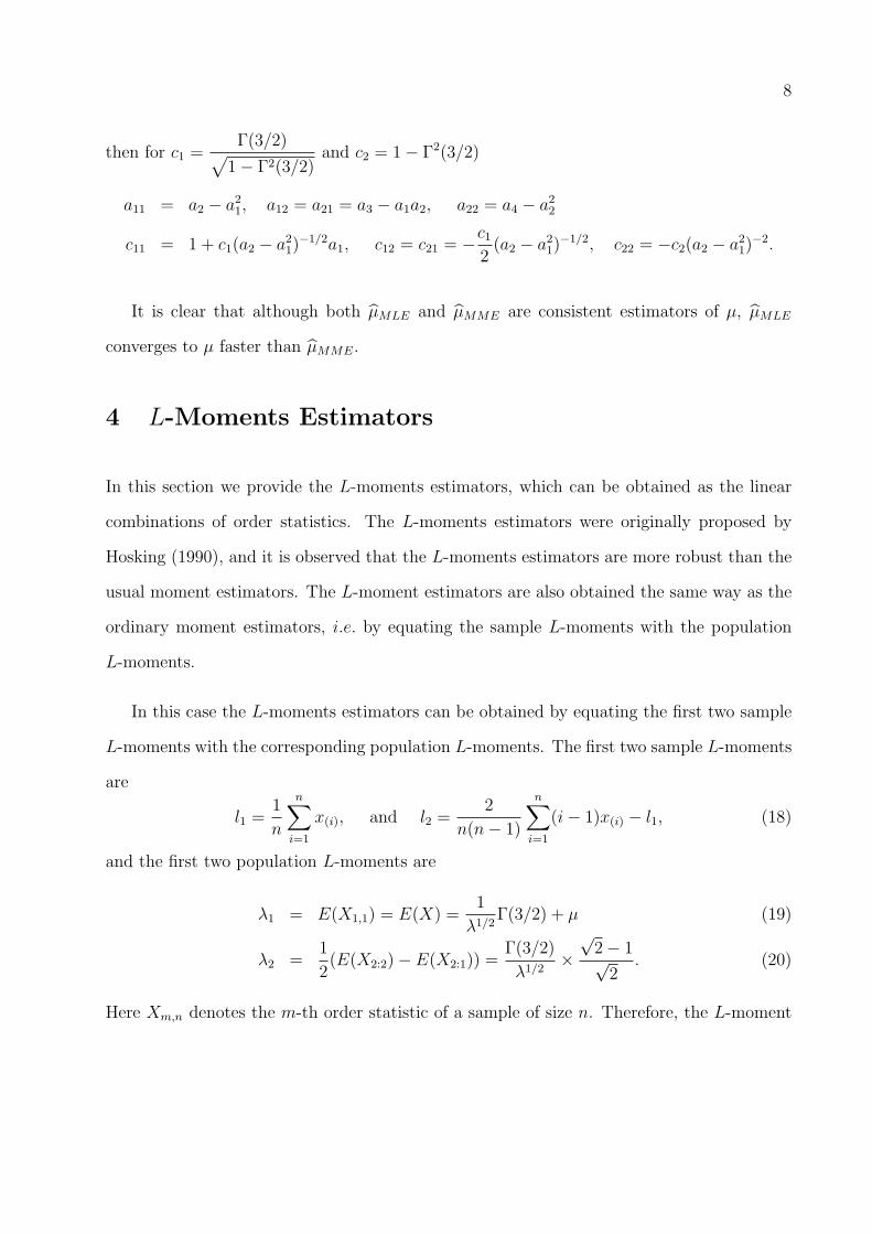
8

then for c1 =Γ(3/2)√

1− Γ2(3/2)and c2 = 1− Γ2(3/2)

a11 = a2 − a21, a12 = a21 = a3 − a1a2, a22 = a4 − a22

c11 = 1 + c1(a2 − a21)−1/2a1, c12 = c21 = −c1

2(a2 − a21)

−1/2, c22 = −c2(a2 − a21)−2.

It is clear that although both µ̂MLE and µ̂MME are consistent estimators of µ, µ̂MLE

converges to µ faster than µ̂MME.

4 L-Moments Estimators

In this section we provide the L-moments estimators, which can be obtained as the linear

combinations of order statistics. The L-moments estimators were originally proposed by

Hosking (1990), and it is observed that the L-moments estimators are more robust than the

usual moment estimators. The L-moment estimators are also obtained the same way as the

ordinary moment estimators, i.e. by equating the sample L-moments with the population

L-moments.

In this case the L-moments estimators can be obtained by equating the first two sample

L-moments with the corresponding population L-moments. The first two sample L-moments

are

l1 =1

n

n∑

i=1

x(i), and l2 =2

n(n− 1)

n∑

i=1

(i− 1)x(i) − l1, (18)

and the first two population L-moments are

λ1 = E(X1,1) = E(X) =1

λ1/2Γ(3/2) + µ (19)

λ2 =1

2(E(X2:2)− E(X2:1)) =

Γ(3/2)

λ1/2×

√2− 1√2

. (20)

Here Xm,n denotes the m-th order statistic of a sample of size n. Therefore, the L-moment

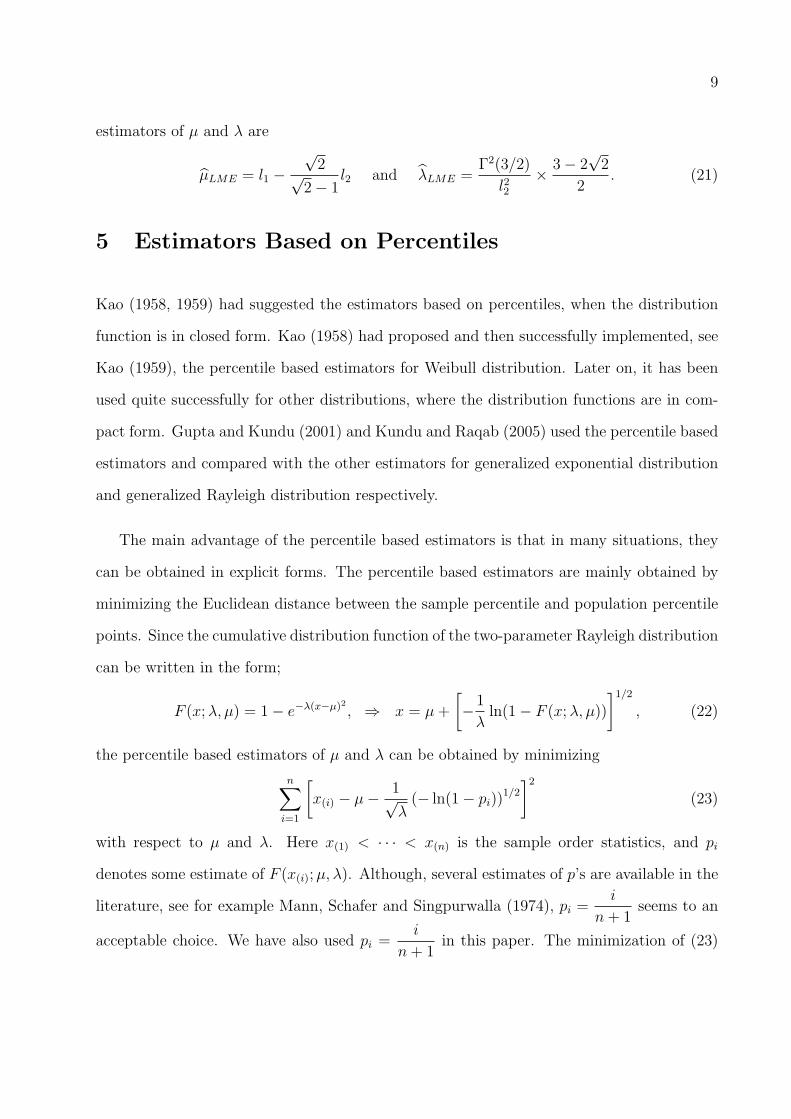
9

estimators of µ and λ are

µ̂LME = l1 −√2√

2− 1l2 and λ̂LME =

Γ2(3/2)

l22× 3− 2

√2

2. (21)

5 Estimators Based on Percentiles

Kao (1958, 1959) had suggested the estimators based on percentiles, when the distribution

function is in closed form. Kao (1958) had proposed and then successfully implemented, see

Kao (1959), the percentile based estimators for Weibull distribution. Later on, it has been

used quite successfully for other distributions, where the distribution functions are in com-

pact form. Gupta and Kundu (2001) and Kundu and Raqab (2005) used the percentile based

estimators and compared with the other estimators for generalized exponential distribution

and generalized Rayleigh distribution respectively.

The main advantage of the percentile based estimators is that in many situations, they

can be obtained in explicit forms. The percentile based estimators are mainly obtained by

minimizing the Euclidean distance between the sample percentile and population percentile

points. Since the cumulative distribution function of the two-parameter Rayleigh distribution

can be written in the form;

F (x;λ, µ) = 1− e−λ(x−µ)2 , ⇒ x = µ+

[−1

λln(1− F (x;λ, µ))

]1/2, (22)

the percentile based estimators of µ and λ can be obtained by minimizing

n∑

i=1

[x(i) − µ− 1√

λ(− ln(1− pi))

1/2

]2(23)

with respect to µ and λ. Here x(1) < · · · < x(n) is the sample order statistics, and pi

denotes some estimate of F (x(i);µ, λ). Although, several estimates of p’s are available in the

literature, see for example Mann, Schafer and Singpurwalla (1974), pi =i

n+ 1seems to an

acceptable choice. We have also used pi =i

n+ 1in this paper. The minimization of (23)

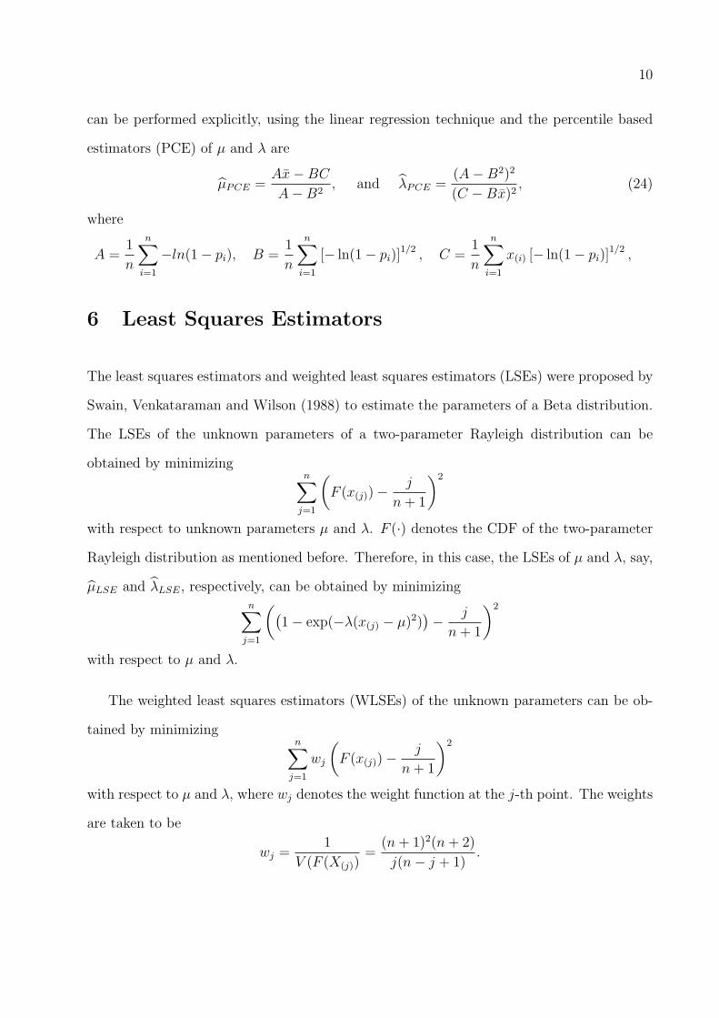
10

can be performed explicitly, using the linear regression technique and the percentile based

estimators (PCE) of µ and λ are

µ̂PCE =Ax̄− BC

A−B2, and λ̂PCE =

(A−B2)2

(C − Bx̄)2, (24)

where

A =1

n

n∑

i=1

−ln(1− pi), B =1

n

n∑

i=1

[− ln(1− pi)]1/2 , C =

1

n

n∑

i=1

x(i) [− ln(1− pi)]1/2 ,

6 Least Squares Estimators

The least squares estimators and weighted least squares estimators (LSEs) were proposed by

Swain, Venkataraman and Wilson (1988) to estimate the parameters of a Beta distribution.

The LSEs of the unknown parameters of a two-parameter Rayleigh distribution can be

obtained by minimizingn∑

j=1

(F (x(j))−

j

n+ 1

)2

with respect to unknown parameters µ and λ. F (·) denotes the CDF of the two-parameter

Rayleigh distribution as mentioned before. Therefore, in this case, the LSEs of µ and λ, say,

µ̂LSE and λ̂LSE, respectively, can be obtained by minimizingn∑

j=1

((1− exp(−λ(x(j) − µ)2)

)− j

n+ 1

)2

with respect to µ and λ.

The weighted least squares estimators (WLSEs) of the unknown parameters can be ob-

tained by minimizingn∑

j=1

wj

(F (x(j))−

j

n+ 1

)2

with respect to µ and λ, where wj denotes the weight function at the j-th point. The weights

are taken to be

wj =1

V (F (X(j))=

(n+ 1)2(n+ 2)

j(n− j + 1).

11

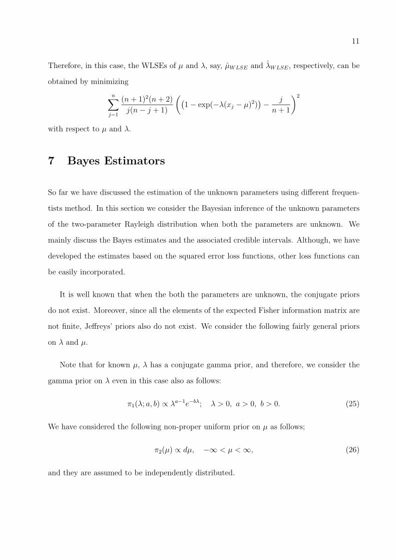
Therefore, in this case, the WLSEs of µ and λ, say, µ̂WLSE and λ̂WLSE, respectively, can be

obtained by minimizing

n∑

j=1

(n+ 1)2(n+ 2)

j(n− j + 1)

((1− exp(−λ(xj − µ)2)

)− j

n+ 1

)2

with respect to µ and λ.

7 Bayes Estimators

So far we have discussed the estimation of the unknown parameters using different frequen-

tists method. In this section we consider the Bayesian inference of the unknown parameters

of the two-parameter Rayleigh distribution when both the parameters are unknown. We

mainly discuss the Bayes estimates and the associated credible intervals. Although, we have

developed the estimates based on the squared error loss functions, other loss functions can

be easily incorporated.

It is well known that when the both the parameters are unknown, the conjugate priors

do not exist. Moreover, since all the elements of the expected Fisher information matrix are

not finite, Jeffreys’ priors also do not exist. We consider the following fairly general priors

on λ and µ.

Note that for known µ, λ has a conjugate gamma prior, and therefore, we consider the

gamma prior on λ even in this case also as follows:

π1(λ; a, b) ∝ λa−1e−bλ; λ > 0, a > 0, b > 0. (25)

We have considered the following non-proper uniform prior on µ as follows;

π2(µ) ∝ dµ, −∞ < µ < ∞, (26)

and they are assumed to be independently distributed.

12

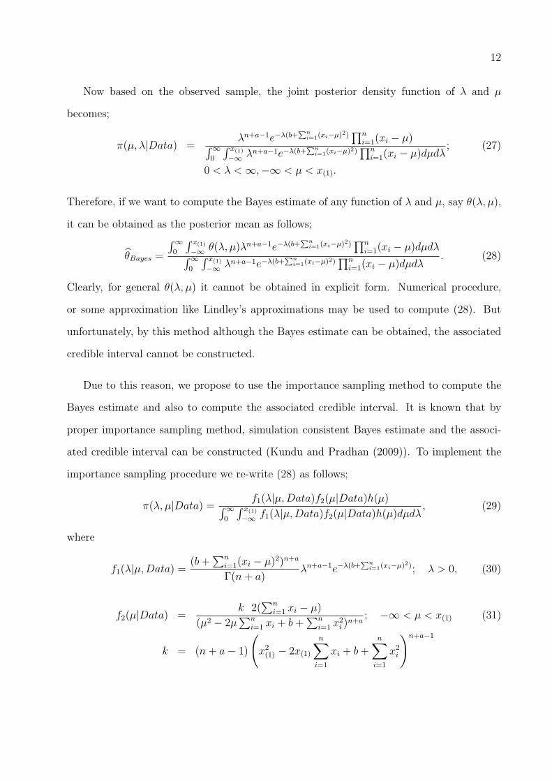
Now based on the observed sample, the joint posterior density function of λ and µ

becomes;

π(µ, λ|Data) =λn+a−1e−λ(b+

∑ni=1(xi−µ)2)

∏ni=1(xi − µ)∫

∞

0

∫ x(1)

−∞λn+a−1e−λ(b+

∑ni=1(xi−µ)2)

∏ni=1(xi − µ)dµdλ

; (27)

0 < λ < ∞,−∞ < µ < x(1).

Therefore, if we want to compute the Bayes estimate of any function of λ and µ, say θ(λ, µ),

it can be obtained as the posterior mean as follows;

θ̂Bayes =

∫∞

0

∫ x(1)

−∞θ(λ, µ)λn+a−1e−λ(b+

∑ni=1(xi−µ)2)

∏ni=1(xi − µ)dµdλ∫

∞

0

∫ x(1)

−∞λn+a−1e−λ(b+

∑ni=1(xi−µ)2)

∏ni=1(xi − µ)dµdλ

. (28)

Clearly, for general θ(λ, µ) it cannot be obtained in explicit form. Numerical procedure,

or some approximation like Lindley’s approximations may be used to compute (28). But

unfortunately, by this method although the Bayes estimate can be obtained, the associated

credible interval cannot be constructed.

Due to this reason, we propose to use the importance sampling method to compute the

Bayes estimate and also to compute the associated credible interval. It is known that by

proper importance sampling method, simulation consistent Bayes estimate and the associ-

ated credible interval can be constructed (Kundu and Pradhan (2009)). To implement the

importance sampling procedure we re-write (28) as follows;

π(λ, µ|Data) =f1(λ|µ,Data)f2(µ|Data)h(µ)∫

∞

0

∫ x(1)

−∞f1(λ|µ,Data)f2(µ|Data)h(µ)dµdλ

, (29)

where

f1(λ|µ,Data) =(b+

∑ni=1(xi − µ)2)n+a

Γ(n+ a)λn+a−1e−λ(b+

∑ni=1(xi−µ)2); λ > 0, (30)

f2(µ|Data) =k 2(

∑ni=1 xi − µ)

(µ2 − 2µ∑n

i=1 xi + b+∑n

i=1 x2i )

n+a; −∞ < µ < x(1) (31)

k = (n+ a− 1)

(x2(1) − 2x(1)

n∑

i=1

xi + b+n∑

i=1

x2i

)n+a−1

13

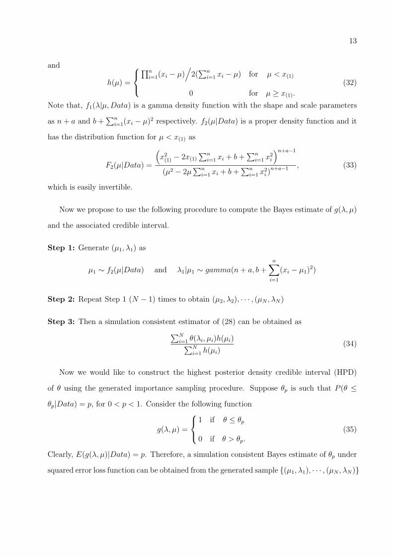
and

h(µ) =

∏ni=1(xi − µ)

/2(∑n

i=1 xi − µ) for µ < x(1)

0 for µ ≥ x(1).

(32)

Note that, f1(λ|µ,Data) is a gamma density function with the shape and scale parameters

as n+ a and b+∑n

i=1(xi − µ)2 respectively. f2(µ|Data) is a proper density function and it

has the distribution function for µ < x(1) as

F2(µ|Data) =

(x2(1) − 2x(1)

∑ni=1 xi + b+

∑ni=1 x

2i

)n+a−1

(µ2 − 2µ∑n

i=1 xi + b+∑n

i=1 x2i )

n+a−1 , (33)

which is easily invertible.

Now we propose to use the following procedure to compute the Bayes estimate of g(λ, µ)

and the associated credible interval.

Step 1: Generate (µ1, λ1) as

µ1 ∼ f2(µ|Data) and λ1|µ1 ∼ gamma(n+ a, b+n∑

i=1

(xi − µ1)2)

Step 2: Repeat Step 1 (N − 1) times to obtain (µ2, λ2), · · · , (µN , λN)

Step 3: Then a simulation consistent estimator of (28) can be obtained as

∑Ni=1 θ(λi, µi)h(µi)∑N

i=1 h(µi)(34)

Now we would like to construct the highest posterior density credible interval (HPD)

of θ using the generated importance sampling procedure. Suppose θp is such that P (θ ≤

θp|Data) = p, for 0 < p < 1. Consider the following function

g(λ, µ) =

1 if θ ≤ θp

0 if θ > θp.(35)

Clearly, E(g(λ, µ)|Data) = p. Therefore, a simulation consistent Bayes estimate of θp under

squared error loss function can be obtained from the generated sample {(µ1, λ1), · · · , (µN , λN)}

14

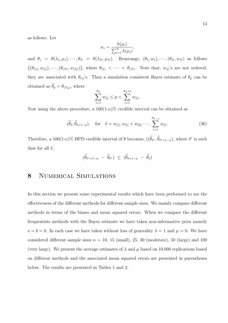
as follows. Let

wi =h(µi)∑Ni=1 h(µi)

,

and θ1 = θ(λ1, µ1), · · · , θN = θ(λN , µN). Rearrange, (θ1, w1), · · · , (θN , wN) as follows

{(θ(1), w[1]), · · · , (θ(N), w[N ])}, where θ(1) < · · · < θ(N). Note that, w[i]’s are not ordered,

they are associated with θ(i)’s. Then a simulation consistent Bayes estimate of θp can be

obtained as θ̂p = θ(Np), whereNp∑

i=1

w[i] ≤ p <

Np+1∑

i=1

w[i].

Now using the above procedure, a 100(1-α)% credible interval can be obtained as

(θ̂δ, θ̂δ+1−α), for δ = w[1], w[1] + w[2], · · · ,N1−α∑

i=1

w[i]. (36)

Therefore, a 100(1-α)% HPD credible interval of θ becomes, ((θ̂δ∗ , θ̂δ∗+1−α), where δ∗ is such

that for all δ,

(θ̂δ∗+1−α − θ̂δ∗) ≤ (θ̂δ+1−α − θ̂δ)

8 Numerical Simulations

In this section we present some experimental results which have been performed to see the

effectiveness of the different methods for different sample sizes. We mainly compare different

methods in terms of the biases and mean squared errors. When we compare the different

frequentists methods with the Bayes estimate we have taken non-informative prior namely

a = b = 0. In each case we have taken without loss of generality λ = 1 and µ = 0. We have

considered different sample sizes n = 10, 15 (small), 25, 30 (moderate), 50 (large) and 100

(very large). We present the average estimates of λ and µ based on 10,000 replications based

on different methods and the associated mean squared errors are presented in parentheses

below. The results are presented in Tables 1 and 2.

15

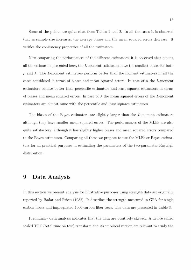
Some of the points are quite cleat from Tables 1 and 2. In all the cases it is observed

that as sample size increases, the average biases and the mean squared errors decrease. It

verifies the consistency properties of all the estimators.

Now comparing the performances of the different estimators, it is observed that among

all the estimators presented here, the L-moment estimators have the smallest biases for both

µ and λ. The L-moment estimators perform better than the moment estimators in all the

cases considered in terms of biases and mean squared errors. In case of µ the L-moment

estimators behave better than percentile estimators and least squares estimators in terms

of biases and mean squared errors. In case of λ the mean squared errors of the L-moment

estimators are almost same with the percentile and least squares estimators.

The biases of the Bayes estimators are slightly larger than the L-moment estimators

although they have smaller mean squared errors. The performances of the MLEs are also

quite satisfactory, although it has slightly higher biases and mean squared errors compared

to the Bayes estimators. Comparing all these we propose to use the MLEs or Bayes estima-

tors for all practical purposes in estimating the parameters of the two-parameter Rayleigh

distribution.

9 Data Analysis

In this section we present analysis for illustrative purposes using strength data set originally

reported by Badar and Priest (1982). It describes the strength measured in GPA for single

carbon fibers and impregnated 1000-carbon fiber tows. The data are presented in Table 3.

Preliminary data analysis indicates that the data are positively skewed. A device called

scaled TTT (total time on test) transform and its empirical version are relevant to study the

16

Table 1: Average estimates of µ and their associated MSE’s.n µ̂MLE µ̂MME µ̂LME µ̂PCE µ̂LSE µ̂BAY ES

10 0.1073 0.0384 0.0113 -0.0620 -0.0328 0.0264(0.0382) (0.0433) (0.0422) (0.0542) (0.0579) (0.0245)

15 0.0713 0.0211 0.0034 -0.0534 -0.0204 0.0248(0.0211) (0.0267) (0.0256) (0.0329) (0.0324) (0.0111)

25 0.0507 0.0153 0.0054 -0.0359 -0.0028 0.0210(0.0117) (0.0167) (0.0159) (0.0194) (0.0182) (0.0051)

30 0.0420 0.0110 0.0003 -0.0357 -0.0113 0.0205(0.0088) (0.0127) (0.0117) (0.0147) (0.0125) (0.0038)

50 0.0226 0.0019 -0.0034 -0.0292 -0.0056 0.0152(0.0042) (0.0082) (0.0075) (0.0094) (0.0077) (0.0022)

100 0.0156 0.0003 -0.0015 -0.0182 -0.0027 0.0137(0.0021) (0.0041) (0.0037) (0.0045) (0.0036) (0.0018)

shape of the hazard function of a distribution function. For a family with survival function

S(y) and distribution function F (y) with positive supports, the scaled TTT transform is

defined for 0 < u < 1, as φF (u) = H−1F (u)/H−1

F (1), where H−1F (u) =

∫ F−1(u)

0

S(y)dy. The

empirical version of the scaled TTT transform for j = 1, . . . , n, is given by

φn(j/n) = H−1n (j/n)/H−1

n (1) =

(j∑

i=1

x(i) + (n− j)x(j)

)/(n∑

i=1

x(i)

),

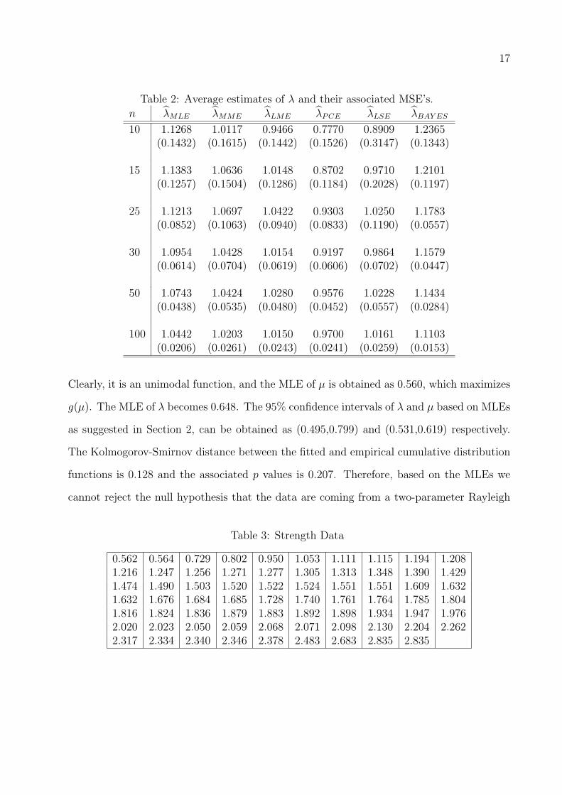
see Aarset (1987). Aarset (1987) showed that the scaled TTT transform is concave (convex)

if the hazard function is increasing (decreasing). To check the shape of the empirical hazard

function, we have plotted the scaled TTT transform in Figure 1. Since it is a concave func-

tion, it indicates that the hazard function of the distribution will be an increasing function.

Therefore, Rayleigh distribution can be used to analyze this data set.

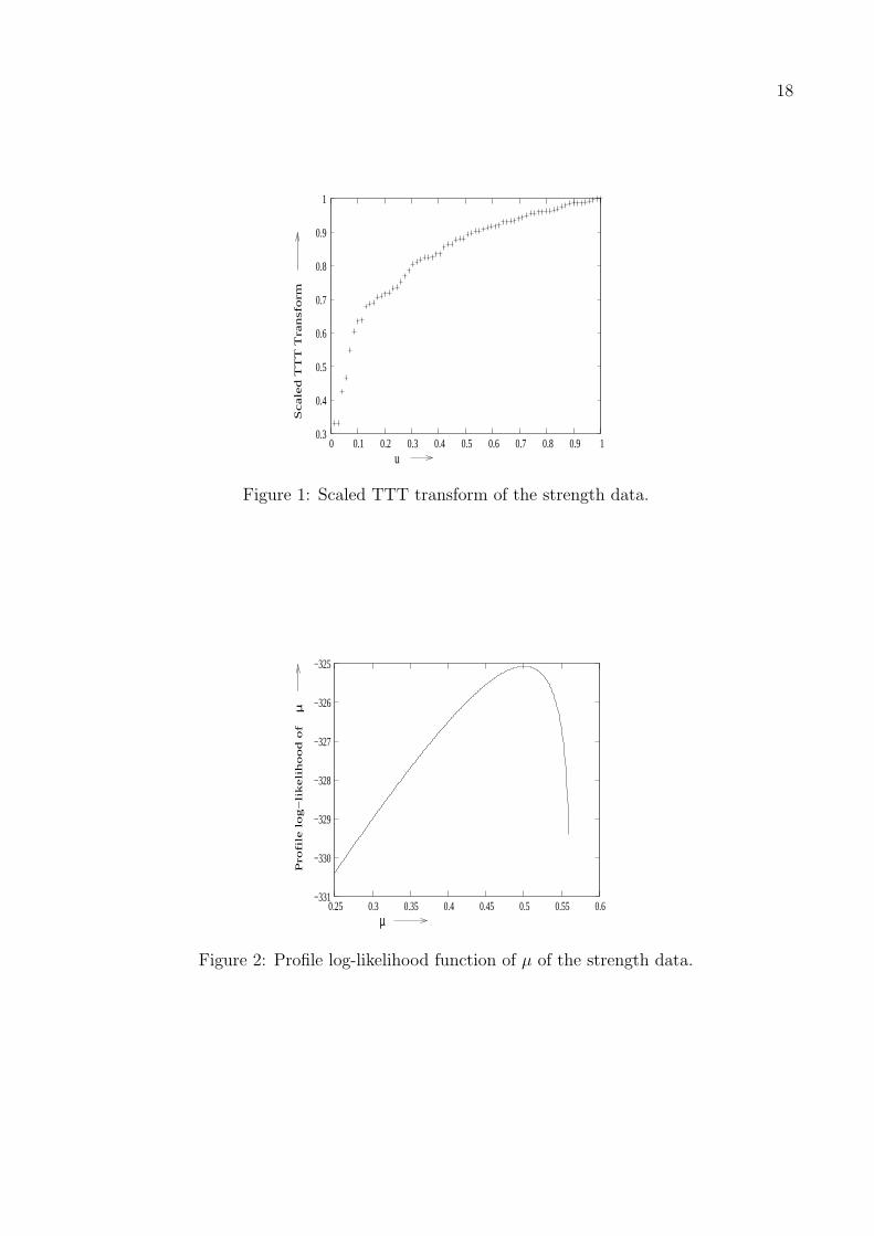
First we would like to compute the maximum likelihood estimators of the unknown

parameters. The profile log-likelihood g(µ) of µ as provided in (7) is provided in Figure 2.

17

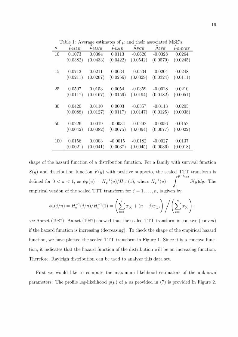
Table 2: Average estimates of λ and their associated MSE’s.

n λ̂MLE λ̂MME λ̂LME λ̂PCE λ̂LSE λ̂BAY ES

10 1.1268 1.0117 0.9466 0.7770 0.8909 1.2365(0.1432) (0.1615) (0.1442) (0.1526) (0.3147) (0.1343)

15 1.1383 1.0636 1.0148 0.8702 0.9710 1.2101(0.1257) (0.1504) (0.1286) (0.1184) (0.2028) (0.1197)

25 1.1213 1.0697 1.0422 0.9303 1.0250 1.1783(0.0852) (0.1063) (0.0940) (0.0833) (0.1190) (0.0557)

30 1.0954 1.0428 1.0154 0.9197 0.9864 1.1579(0.0614) (0.0704) (0.0619) (0.0606) (0.0702) (0.0447)

50 1.0743 1.0424 1.0280 0.9576 1.0228 1.1434(0.0438) (0.0535) (0.0480) (0.0452) (0.0557) (0.0284)

100 1.0442 1.0203 1.0150 0.9700 1.0161 1.1103(0.0206) (0.0261) (0.0243) (0.0241) (0.0259) (0.0153)

Clearly, it is an unimodal function, and the MLE of µ is obtained as 0.560, which maximizes

g(µ). The MLE of λ becomes 0.648. The 95% confidence intervals of λ and µ based on MLEs

as suggested in Section 2, can be obtained as (0.495,0.799) and (0.531,0.619) respectively.

The Kolmogorov-Smirnov distance between the fitted and empirical cumulative distribution

functions is 0.128 and the associated p values is 0.207. Therefore, based on the MLEs we

cannot reject the null hypothesis that the data are coming from a two-parameter Rayleigh

Table 3: Strength Data

0.562 0.564 0.729 0.802 0.950 1.053 1.111 1.115 1.194 1.2081.216 1.247 1.256 1.271 1.277 1.305 1.313 1.348 1.390 1.4291.474 1.490 1.503 1.520 1.522 1.524 1.551 1.551 1.609 1.6321.632 1.676 1.684 1.685 1.728 1.740 1.761 1.764 1.785 1.8041.816 1.824 1.836 1.879 1.883 1.892 1.898 1.934 1.947 1.9762.020 2.023 2.050 2.059 2.068 2.071 2.098 2.130 2.204 2.2622.317 2.334 2.340 2.346 2.378 2.483 2.683 2.835 2.835

18

u

Sca

led

TT

T T

ran

sfo

rm

0.3

0.4

0.5

0.6

0.7

0.8

0.9

1

0 0.1 0.2 0.3 0.4 0.5 0.6 0.7 0.8 0.9 1

Figure 1: Scaled TTT transform of the strength data.

µ

Pro

file

lo

g−

like

lih

oo

d o

fµ

−331

−330

−329

−328

−327

−326

−325

0.25 0.3 0.35 0.4 0.45 0.5 0.55 0.6

Figure 2: Profile log-likelihood function of µ of the strength data.

19

distribution.

To compute the Bayes estimates we have assumed non-informative priors namely a = b =

c = d = 0. Based on 1,000 importance sampling we obtain the Bayes estimates of µ and λ

as 0.543 and 0.629 respectively. The 95% symmetric credible intervals of λ and µ are (0.445,

0.798) and (0.530, 0.562) respectively. The Kolmogorov-Smirnov distance between the fitted

and empirical cumulative distribution functions is 0.130 and the associated p values is 0.191.

Therefore, Bayes estimates also provide satisfactory goodness of fit of the two-parameter

Rayleigh distribution to the strength data.

10 Conclusions

In this paper we have considered different estimation procedures for estimating the unknown

location and scale parameters of a two-parameter Rayleigh distribution. We have mainly

considered the maximum likelihood estimators, the method of moment estimators, the L-

moment estimators, percentile estimators, least squares estimators and the Bayes estimators.

It is not possible to compare different methods theoretically, and we have used some simu-

lations to compare different estimators. We have compared different estimators mainly with

respect to biases and mean squared errors. It is observed that the Bayes estimators with

non-informative priors work very well in terms of biases and mean squared errors, although

it is quite involved computationally. The performances of the maximum likelihood estima-

tors are also quite satisfactory. We recommend use of the MLEs or Bayes estimators for all

practical purposes.

20

Acknowledgments

The authors would like to thank the editors and the reviewers who helped to substantially

improve the paper. The authors are thankful to Professor R.G. Surles for providing the

strength data.

References

[1] Abd-Elfattah, A. M., Hassan, A. S. & Ziedan, D. M. (2006). Efficiency of maximum

likelihood estimators under different censored sampling schemes for Rayleigh distribution.

Interstat, March issue, 1.

[2] Aarset, M.V. (1987). How to identify a bathtub shaped hazard rate?. IEEE Transactions

on Reliability, 36, 106 - 108.

[3] Badar, M.G. & Priest, A.M. (1982). Statistical aspects of fiber and bundle strength in

hybrids composite. Progress in Science and Engineering Composites (T. Hayakashi, K.

Kawata & S. Umekawa eds.), ICCM-IV, Tokyo, 1129 - 1136.

[4] Dey, S. (2009). Comparison of Bayes Estimators of the parameter and reliability function

for Rayleigh distribution under different loss functions. Malaysian Journal of Mathemat-

ical Sciences, 3, 247 - 264.

[5] Dey, S. & Das, M.K. (2007). A Note on Prediction Interval for a Rayleigh Distribution:

Bayesian Approach. American Journal of Mathematical and Management Science, 1&2,

43 - 48.

[6] Gupta, R.D. & Kundu, D. (2001). Generalized exponential distributions: different meth-

ods of estimation. Journal of Statistical Computation and Simulation, 69, 315 - 338.

21

[7] Hosking, J.R.M. (1990). L-moment: analysis and estimation of distributions using linear

combinations of order statistics. Journal of Royal Statistical Society, Ser. B, 52, 105 -

124.

[8] Johnson, N.L., Kotz, S. & Balakrishnan, N. (1994). Continuous Univariate Distribution

(Volume 1). John Wiley & Sons, New York.

[9] Kao, J.H.K. (1958). Computer methods for estimating Weibull parameters in reliability

studies. Trans. IRE Reliability Quality Control, 13, 15 - 22.

[10] Kao, J.H.K. (1959). A graphical estimation of mixed Weibull parameters in life testing

electron tube. Technometrics, 1, 389 - 407.

[11] Khan, H.M.R., Provost, S.B. & Singh, A. (2010). Predictive inference from a two-

parameter Rayleigh life model given a doubly censored sample. Communications in

Statistics - Theory and Methods, 39, 1237 - 1246.

[12] Kundu, D. & Raqab, M.Z. (2005). Generalized Rayleigh distribution: different methods

of estimation. Computational Statistics and Data Analysis, 49, 187 - 200.

[13] Rayleigh, J.W.S. (1880). On the resultant of a large number of vibrations of the some

pitch and of arbitrary phase. Philosophical Magazine, 5-th Series, 10, 73 - 78.

[14] Smith, R.L. (1995). Maximum likelihood estimation in a class of non-regular cases.

Biometrika, 72, 67 - 90.

[15] Swain, J.J., Venkataraman, S. & Wilson, J.R. (1988). Least squares estimation of dis-

tribution functions in Johnson’s translation system. Journal of Statistical Computation

and Simulation, 29, 271 - 297.