Two Models of FX Market Interventions: The Cases of … · Two Models of FX Market Interventions:...
36
Banco de México Documentos de Investigación Banco de México Working Papers N° 2016-14 Two Models of FX Market Interventions: The Cases of Brazil and Mexico August 2016 La serie de Documentos de Investigación del Banco de México divulga resultados preliminares de trabajos de investigación económica realizados en el Banco de México con la finalidad de propiciar el intercambio y debate de ideas. El contenido de los Documentos de Investigación, así como las conclusiones que de ellos se derivan, son responsabilidad exclusiva de los autores y no reflejan necesariamente las del Banco de México. The Working Papers series of Banco de México disseminates preliminary results of economic research conducted at Banco de México in order to promote the exchange and debate of ideas. The views and conclusions presented in the Working Papers are exclusively the responsibility of the authors and do not necessarily reflect those of Banco de México. Martín Tobal Banco de México Renato Yslas Banco de México
-
Upload
truongdiep -
Category
Documents
-
view
214 -
download
0
Transcript of Two Models of FX Market Interventions: The Cases of … · Two Models of FX Market Interventions:...
Banco de México
Documentos de Investigación
Banco de México
Working Papers
N° 2016-14
Two Models of FX Market Interventions: The Cases of
Brazil and Mexico
August 2016
La serie de Documentos de Investigación del Banco de México divulga resultados preliminares de
trabajos de investigación económica realizados en el Banco de México con la finalidad de propiciar elintercambio y debate de ideas. El contenido de los Documentos de Investigación, así como lasconclusiones que de ellos se derivan, son responsabilidad exclusiva de los autores y no reflejannecesariamente las del Banco de México.
The Working Papers series of Banco de México disseminates preliminary results of economicresearch conducted at Banco de México in order to promote the exchange and debate of ideas. Theviews and conclusions presented in the Working Papers are exclusively the responsibility of the authorsand do not necessarily reflect those of Banco de México.
Mart ín TobalBanco de México
Renato YslasBanco de México
Two Models of FX Market Intervent ions: The Cases ofBrazi l and Mexico*
Abstract: This paper empirically compares the implications of two distinct models of FXintervention, within the context of Inflation Targeting Regimes. For this purpose, it applies the VARmethodology developed by Kim (2003) to the cases of Mexico and Brazil. Our results can besummarized in three points. First, FX interventions have had a short-lived effect on the exchange rate inboth economies. Second, the Brazilian model of FX intervention entails higher inflationary costs andthis result cannot be entirely explained by differences in the level of pass-through. Third, each model isassociated with a different interaction between exchange rate and interest rate setting (conventionalmonetary policies).Keywords: Foreign exchange intervention; Exchange rate pass-through; Exchange rate regime;Monetary policy coordination.JEL Classification: F31; E31; E52.
Resumen: Este documento compara empíricamente las implicaciones de dos modelos distintos deintervención cambiaria, en un contexto de regímenes de metas de inflación. Con este fin, el documentoaplica la metodología VAR desarrollada por Kim (2003) a los casos de México y Brasil. Los resultadospueden resumirse fácilmente en tres puntos. Primero, las intervenciones cambiarias han tenido efectos decorta duración sobre el tipo de cambio en ambas economías. Segundo, el modelo de intervencióncambiaria brasileño acarrea mayores costos de inflación e, interesantemente, este resultado no puede serenteramente explicado por diferencias en el nivel de traspaso de tipo de cambio a precios. Tercero, cadauno de los modelos posee implicaciones distintas para la interacción entre política de tipo de cambio ytasa de interés (política monetaria convencional).Palabras Clave: Intervención cambiaria; Traspaso del tipo de cambio; Régimen Cambiario;Coordinación de la política monetaria.
Documento de Investigación2016-14
Working Paper2016-14
Mart ín Toba l yBanco de México
Renato Ys las z
Banco de México
*The opinions expressed in this publication are those of the authors. They do not purport to reflect the opinionsor views of Banco de México or its Board of Governors. We would like to thank for valuable comments João Barata Ribeiro Blanco Barroso, Fernando Tenjo, Daniel Chiquiar, Alberto Ortiz, Nicolás Magud, Fabricio Orrego, Julio Carrillo, Fernando Avalos, Santiago Garcia-Verdú, Victoria Nuguer and other participants of the Meeting of the Central Bank Joint Research of the Americas. Please address e-mail correspondence to: [email protected] y Dirección General de Investigación Económica, Banco de México. Email: [email protected]. z Dirección General de Estabilidad Financiera, Banco de México. Email: [email protected].
1
1. Introduction
Historically, Latin America has seen a wide range of choices in terms of exchange rate and
monetary policy regimes. Since the early 2000s a number of countries have opted for an
Inflation Targeting Regime and devoted interest rate setting to meet the target. During this
period, the goal of monetary policy has been almost exclusively to keep inflation under
control. However, inflation targets and interest rate setting have come with varying degrees
of exchange rate flexibility: Latin-American economies currently perform foreign exchange
(FX) interventions under substantially different models. This paper investigates whether a
country's choice of FX intervention model constrains their impact on the exchange rate, the
country's inflation rate, and the nature of interaction between exchange rate and conventional
monetary policies (interest rate setting). For this purpose, it uses the vector autoregression
(VAR) model developed by Kim (2003) to compare the cases of Mexico and Brazil, two
inflation targeting countries with distinct models of FX intervention.
When asked about the exchange rate policies followed by Mexico and Brazil, most
economists would probably classify them as managed floating policies (see Ilzetzki et al.,
2008; Tobal, 2013 and IMF, 2015 for alternative exchange rate regime classifications).1
However, as illustrated in Figures 1-2, using a single category for both countries would hide
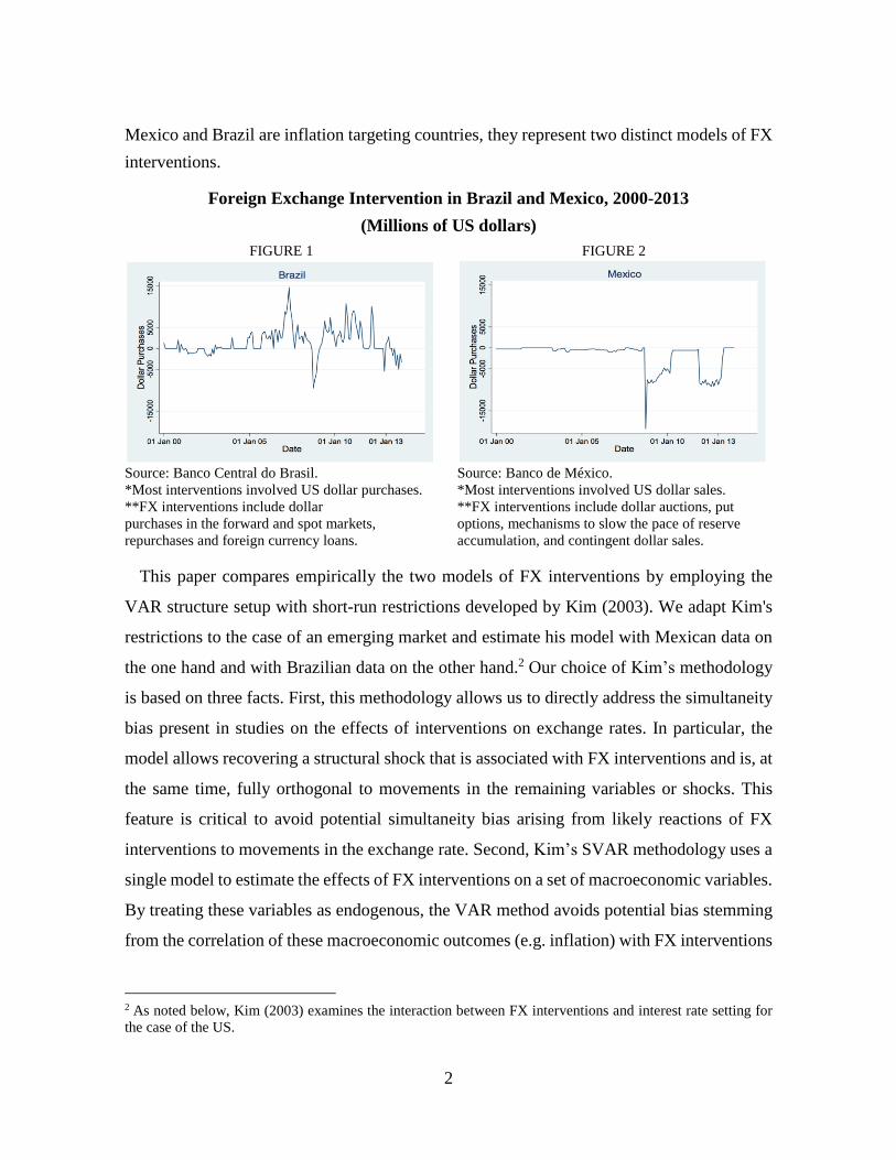
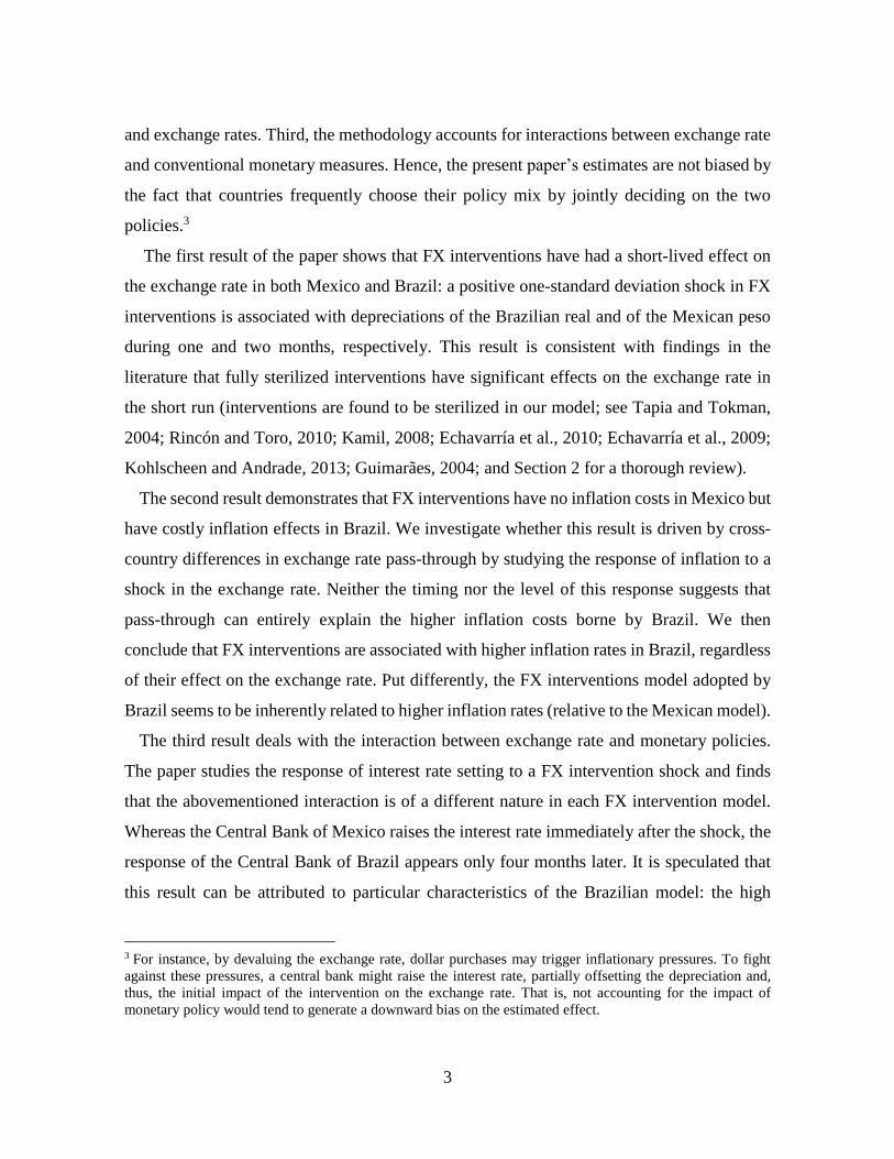
substantial differences across the two emerging markets. Figure 1 shows that the majority of
Brazilian interventions have involved net dollar purchases and, importantly, they have been
performed on a regular basis. On the other hand, the majority of Mexican interventions have
involved net dollar sales and interventions have been more sporadic (mostly in the aftermath
of the 2008-2009 financial crisis). Moreover, whereas Mexico has followed a pre-established
rule, Brazil has primarily used discretionary interventions. In summary, although both
1 The IMF Annual Report on Exchange Arrangements and Exchange Restrictions (2015) classifies both
economies as inflation-targeters. As for their exchange rate regimes, there exists some variation. Ilzetzki et al.
(2008) extend Reinhart and Rogoff´s classification of de facto exchange rate regimes for the period 2000-2010
and find that, over this period, both Brazil and Mexico had managed floating regimes. In a different paper,
Tobal (2013) conducts a survey and assembles a unique database on foreign currency risk and exchange rate
regimes. Using this information, he constructs an alternative classification based on self-report perceptions of
regimes for seventeen Latin America and the Caribbean economies. According to this database, Brazil and
Mexico had pegged float exchange rate regimes over the period 2000-2012. In an expanded classification that
accounts for regulatory measures, Tobal (2013) reclassifies the Brazilian regime as foreign exchange controls
over 2000 Q1 – 2005 Q2 to capture the existence of two regulated FX markets. Finally, in the IMF annual report
(2015), the Brazilian and Mexican regimes are classified as floating and free floating, respectively.
2
Mexico and Brazil are inflation targeting countries, they represent two distinct models of FX
interventions.
Foreign Exchange Intervention in Brazil and Mexico, 2000-2013
(Millions of US dollars)
FIGURE 1 FIGURE 2
Source: Banco Central do Brasil. Source: Banco de México.
*Most interventions involved US dollar purchases. *Most interventions involved US dollar sales.
**FX interventions include dollar **FX interventions include dollar auctions, put
purchases in the forward and spot markets, options, mechanisms to slow the pace of reserve
repurchases and foreign currency loans. accumulation, and contingent dollar sales.
This paper compares empirically the two models of FX interventions by employing the
VAR structure setup with short-run restrictions developed by Kim (2003). We adapt Kim's
restrictions to the case of an emerging market and estimate his model with Mexican data on
the one hand and with Brazilian data on the other hand.2 Our choice of Kim’s methodology
is based on three facts. First, this methodology allows us to directly address the simultaneity
bias present in studies on the effects of interventions on exchange rates. In particular, the
model allows recovering a structural shock that is associated with FX interventions and is, at
the same time, fully orthogonal to movements in the remaining variables or shocks. This
feature is critical to avoid potential simultaneity bias arising from likely reactions of FX
interventions to movements in the exchange rate. Second, Kim’s SVAR methodology uses a
single model to estimate the effects of FX interventions on a set of macroeconomic variables.
By treating these variables as endogenous, the VAR method avoids potential bias stemming
from the correlation of these macroeconomic outcomes (e.g. inflation) with FX interventions
2 As noted below, Kim (2003) examines the interaction between FX interventions and interest rate setting for
the case of the US.
3
and exchange rates. Third, the methodology accounts for interactions between exchange rate
and conventional monetary measures. Hence, the present paper’s estimates are not biased by
the fact that countries frequently choose their policy mix by jointly deciding on the two
policies.3
The first result of the paper shows that FX interventions have had a short-lived effect on
the exchange rate in both Mexico and Brazil: a positive one-standard deviation shock in FX
interventions is associated with depreciations of the Brazilian real and of the Mexican peso
during one and two months, respectively. This result is consistent with findings in the
literature that fully sterilized interventions have significant effects on the exchange rate in
the short run (interventions are found to be sterilized in our model; see Tapia and Tokman,
2004; Rincón and Toro, 2010; Kamil, 2008; Echavarría et al., 2010; Echavarría et al., 2009;
Kohlscheen and Andrade, 2013; Guimarães, 2004; and Section 2 for a thorough review).
The second result demonstrates that FX interventions have no inflation costs in Mexico but
have costly inflation effects in Brazil. We investigate whether this result is driven by cross-
country differences in exchange rate pass-through by studying the response of inflation to a
shock in the exchange rate. Neither the timing nor the level of this response suggests that
pass-through can entirely explain the higher inflation costs borne by Brazil. We then
conclude that FX interventions are associated with higher inflation rates in Brazil, regardless
of their effect on the exchange rate. Put differently, the FX interventions model adopted by
Brazil seems to be inherently related to higher inflation rates (relative to the Mexican model).
The third result deals with the interaction between exchange rate and monetary policies.
The paper studies the response of interest rate setting to a FX intervention shock and finds
that the abovementioned interaction is of a different nature in each FX intervention model.
Whereas the Central Bank of Mexico raises the interest rate immediately after the shock, the
response of the Central Bank of Brazil appears only four months later. It is speculated that
this result can be attributed to particular characteristics of the Brazilian model: the high
3 For instance, by devaluing the exchange rate, dollar purchases may trigger inflationary pressures. To fight
against these pressures, a central bank might raise the interest rate, partially offsetting the depreciation and,
thus, the initial impact of the intervention on the exchange rate. That is, not accounting for the impact of
monetary policy would tend to generate a downward bias on the estimated effect.
4
frequency with which the interventions are performed in this country may make it harder to
change the interest rate in response to every inflationary pressure. In particular, the high
frequency of the FX interventions may make it harder to accompany each of them with
increases in the interest rate to offset its inflationary consequences. One implication is that,
within the context of the Brazilian model, the relationship between conventional monetary
policy and inflation rate becomes substantially noisier. At the same time, the later response
of the interest rate to FX interventions in Brazil partially explains the second result, according
to which these interventions entail higher inflationary costs.
As more thoroughly explained in Section 2, this paper makes two main contributions to
studies that investigate the effectiveness of FX interventions in Mexico and Brazil. First, we
base our study on a single model for conventional monetary policy, FX interventions, and
exchange rate. From a methodological point of view, this contribution is relevant because FX
interventions, monetary policy, and exchange rate interact with each other and not accounting
for this interaction may generate sizable bias (Kim, 2003). Second, we compare the two
countries and assess the implications of choosing different models of FX interventions.
The rest of the paper is organized as follows. Section 2 reviews the related literature and
highlights the contributions of this paper to the literature. Section 3 explains the data, the
methodology, and the identifying assumptions employed in the analysis. Section 4 discusses
the empirical results and Section 5 examines the robustness of the results. Finally, section 6
concludes.
2. Related Literature
This paper relates to a set of studies investigating whether sterilized FX interventions are
effective in influencing the level and volatility of the exchange rate. To investigate this issue,
the literature has primarily employed single equation econometric models such as GARCH
specifications, cross-country studies, and event study approaches. Overall, the literature is
not conclusive on the effectiveness of FX interventions. Whereas some papers support the
idea that FX interventions are effective solely in the short run, others find no evidence of
significant effects (see Sarno and Taylor, 2001; Neely, 2005 and Menkhoff, 2013) for
literature reviews).
5
For the particular case of Latin America, most studies show that FX interventions affect
the level of the exchange rate in the short-run but are mixed about their effects on volatility
(see Tapia and Tokman, 2004; Domaç and Mendoza, 2004; Kamil, 2008; Rincón and Toro,
2010; Adler and Tovar, 2011; Kohlscheen and Andrade, 2013; Broto, 2013; García-Verdú
and Zerecero, 2014 and García-Verdú and Ramos-Francia, 2014). For Brazil, Stone et al.
(2009) show that measures aimed at providing liquidity to the FX market affect the level and
volatility of the Brazilian Real/US dollar rate.4 Kohlscheen and Andrade (2013) use intraday
data to demonstrate that a central bank’s offer to buy currency swaps appreciates the
exchange rate in Brazil.5 For Mexico, Domaç and Mendoza (2004) find that dollar sales by
the Central Bank appreciate the peso and have a negative impact on its volatility, while dollar
purchases are found to be not statistically significant. In contrast, Broto (2013) employs a
larger period (July 21, 1996–June 6, 2011) to show that both foreign currency purchases and
sales are associated with lower exchange rate volatility. García-Verdú and Zerecero (2014)
investigate the effects of dollar auctions without a minimum price on liquidity and orderly
conditions. They show that, when these conditions are measured by bid-ask spreads, the
aforementioned auctions improve liquidity and promote order in the FX market.6 García-
Verdú and Ramos-Francia (2014) take a lower frequency approach and use intraday data to
investigate the consequences of FX interventions. Their result show that the effects of FX
interventions on exchange rate risk-neutral densities are statistically little.7
In contrast with the studies on the effectiveness of FX interventions mentioned above, this
paper does not employ a uni-equational econometric model for the exchange rate. Instead,
we analyze this issue in a unifying framework for FX interventions, monetary policy,
exchange rate, and inflation (among other variables). This is relevant because, as argued by
Kim (2003), the two types of policies and the exchange rate interact with each other.
4 Stone et al. (2009) study measures taken in the aftermath of the 2008-2009 financial crisis. They find that spot
dollar sales and the announcements on futures market intervention appreciate the local currency. 5 Note that by selling a currency swap to the Central Bank, the financial institution receives the equivalent of
the exchange rate variation plus a local onshore US interest rate. This reduces its demand for foreign currency,
consequently appreciating the exchange rate. 6 The interventions considered by García-Verdú and Zerecero (2014) lasted five minutes. They show that this
modality of intervention is associated with a lower bid-ask spread of the peso/dollar exchange rate. 7 García-Verdú and Ramos-Francia (2014) use options data to estimate the exchange rate risk-neutral densities.
6
The paper also relates closely to a strand of literature that estimates a rich set of
macroeconomic relationships and interactions between FX interventions and conventional
monetary policy (see Kim, 2003; Guimarães, 2004; and Echavarría et al., 2009). To estimate
these relationships, the literature employs structural VAR frameworks with short-run
restrictions. For instance, Kim (2003) uses monthly data to show that net purchases of foreign
currency substantially depreciate the exchange rate in the US. He also finds that even if these
purchases are sterilized, they have significant effects on monetary variables in the medium
run. Following Kim's framework (2003), Echavarría et al. (2009) jointly analyze the effects
of FX intervention and conventional monetary policy on the exchange rate, interest rate, and
other macroeconomic variables for Colombia. They show that foreign currency purchases
devalue the nominal exchange rate over 1 month.8
In line with the VAR literature on FX interventions outlined above, this paper estimates
the effects of interventions on a broader set of macroeconomic variables (including inflation
and interest rates). In contrast with Kim (2003), Guimarães (2004), and Echavarría et al.
(2009), we estimate these effects for two countries (Brazil and Mexico) that follow different
models of intervention and analyze the implications of such differences in terms of inflation
costs and interactions between FX intervention and conventional monetary policies.
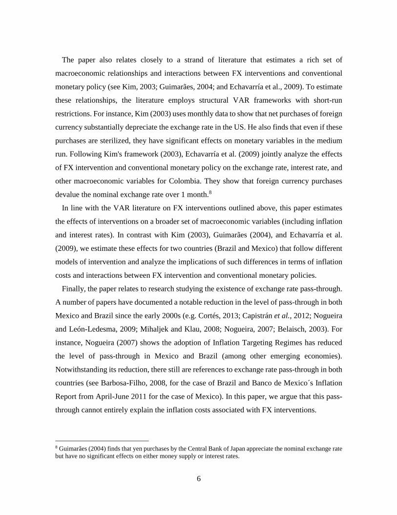
Finally, the paper relates to research studying the existence of exchange rate pass-through.
A number of papers have documented a notable reduction in the level of pass-through in both
Mexico and Brazil since the early 2000s (e.g. Cortés, 2013; Capistrán et al., 2012; Nogueira
and León-Ledesma, 2009; Mihaljek and Klau, 2008; Nogueira, 2007; Belaisch, 2003). For
instance, Nogueira (2007) shows the adoption of Inflation Targeting Regimes has reduced
the level of pass-through in Mexico and Brazil (among other emerging economies).
Notwithstanding its reduction, there still are references to exchange rate pass-through in both
countries (see Barbosa-Filho, 2008, for the case of Brazil and Banco de Mexico´s Inflation
Report from April-June 2011 for the case of Mexico). In this paper, we argue that this pass-
through cannot entirely explain the inflation costs associated with FX interventions.
8 Guimarães (2004) finds that yen purchases by the Central Bank of Japan appreciate the nominal exchange rate
but have no significant effects on either money supply or interest rates.
7
3. Data and Methodology
3.1. Variable Definition and Structural VAR with Short Run Restrictions
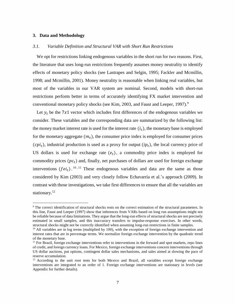
We opt for restrictions linking endogenous variables in the short run for two reasons. First,
the literature that uses long-run restrictions frequently assumes money neutrality to identify
effects of monetary policy shocks (see Lastrapes and Selgin, 1995; Fackler and Mcmillin,
1998; and Mcmillin, 2001). Money neutrality is reasonable when linking real variables, but
most of the variables in our VAR system are nominal. Second, models with short-run
restrictions perform better in terms of accurately identifying FX market intervention and
conventional monetary policy shocks (see Kim, 2003, and Faust and Leeper, 1997).9
Let 𝑦𝑡 be the 7𝑥1 vector which includes first differences of the endogenous variables we
consider. These variables and the corresponding data are summarized by the following list:
the money market interest rate is used for the interest rate (𝑖𝑡), the monetary base is employed
for the monetary aggregate (𝑚𝑡), the consumer price index is employed for consumer prices
(𝑐𝑝𝑖𝑡), industrial production is used as a proxy for output (𝑖𝑝𝑡), the local currency price of
US dollars is used for exchange rate (𝑒𝑡) , a commodity price index is employed for
commodity prices (𝑝𝑐𝑡) and, finally, net purchases of dollars are used for foreign exchange
interventions (𝑓𝑒𝑖𝑡) . 10 , 11 These endogenous variables and data are the same as those
considered by Kim (2003) and very closely follow Echavarría et al.’s approach (2009). In
contrast with those investigations, we take first differences to ensure that all the variables are
stationary.12
9 The correct identification of structural shocks rests on the correct estimation of the structural parameters. In
this line, Faust and Leeper (1997) show that inferences from VARs based on long run assumptions might not
be reliable because of data limitations. They argue that the long-run effects of structural shocks are not precisely
estimated in small samples, and this inaccuracy transfers to impulse-response exercises. In other words,
structural shocks might not be correctly identified when assuming long-run restrictions in finite samples. 10 All variables are in log terms (multiplied by 100), with the exception of foreign exchange intervention and
interest rates that are in percentage terms. We normalize foreign exchange intervention by the quadratic trend
of the monetary base. 11 For Brazil, foreign exchange interventions refer to interventions in the forward and spot markets, repo lines
of credit, and foreign currency loans. For Mexico, foreign exchange interventions concern interventions through
US dollar auctions, put options, contingent dollar sales mechanisms, and sales aimed at slowing the pace of
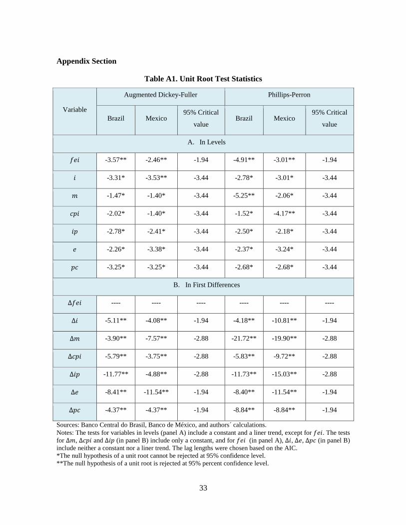
reserve accumulation. 12 According to the unit root tests for both Mexico and Brazil, all variables except foreign exchange
interventions are integrated to an order of 1. Foreign exchange interventions are stationary in levels (see
Appendix for further details).
8
The period under interest is defined to comprise the “Inflation Targeting” period and we
use monthly data (“high-frequency information”) to capture the impact of FX market
interventions on the exchange rate. The sample period is thus defined as 2000M1-2013M12.
The data come from different sources: the Banco Central do Brasil, the International
Financial Statistics of the IMF, and the Banco de México.
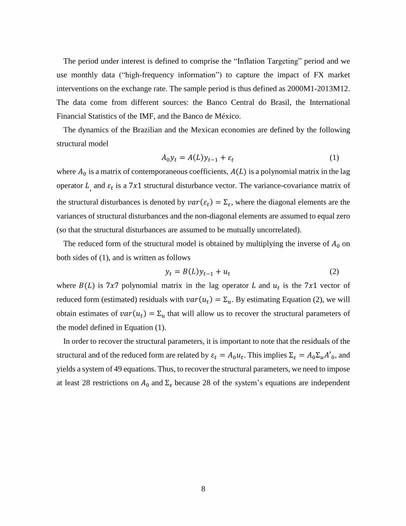
The dynamics of the Brazilian and the Mexican economies are defined by the following
structural model
𝐴0𝑦𝑡 = 𝐴(𝐿)𝑦𝑡−1 + 𝜀𝑡 (1)
where 𝐴0 is a matrix of contemporaneous coefficients, 𝐴(𝐿) is a polynomial matrix in the lag
operator 𝐿, and 𝜀𝑡 is a 7𝑥1 structural disturbance vector. The variance-covariance matrix of
the structural disturbances is denoted by 𝑣𝑎𝑟(𝜀𝑡) = Σ𝜀, where the diagonal elements are the
variances of structural disturbances and the non-diagonal elements are assumed to equal zero
(so that the structural disturbances are assumed to be mutually uncorrelated).
The reduced form of the structural model is obtained by multiplying the inverse of 𝐴0 on
both sides of (1), and is written as follows
𝑦𝑡 = 𝐵(𝐿)𝑦𝑡−1 + 𝑢𝑡 (2)
where 𝐵(𝐿) is 7𝑥7 polynomial matrix in the lag operator 𝐿 and 𝑢𝑡 is the 7𝑥1 vector of
reduced form (estimated) residuals with 𝑣𝑎𝑟(𝑢𝑡) = Σ𝑢. By estimating Equation (2), we will
obtain estimates of 𝑣𝑎𝑟(𝑢𝑡) = Σ𝑢 that will allow us to recover the structural parameters of
the model defined in Equation (1).
In order to recover the structural parameters, it is important to note that the residuals of the
structural and of the reduced form are related by 𝜀𝑡 = 𝐴0𝑢𝑡. This implies Σ𝜀 = 𝐴0Σ𝑢𝐴′0, and
yields a system of 49 equations. Thus, to recover the structural parameters, we need to impose
at least 28 restrictions on 𝐴0 and Σ𝜀 because 28 of the system’s equations are independent
9
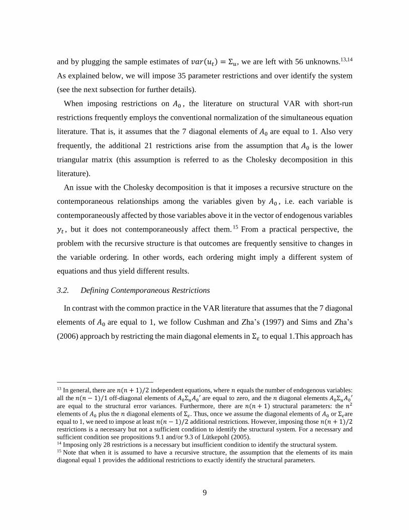
and by plugging the sample estimates of 𝑣𝑎𝑟(𝑢𝑡) = Σ𝑢, we are left with 56 unknowns.13,14
As explained below, we will impose 35 parameter restrictions and over identify the system
(see the next subsection for further details).
When imposing restrictions on 𝐴0 , the literature on structural VAR with short-run
restrictions frequently employs the conventional normalization of the simultaneous equation
literature. That is, it assumes that the 7 diagonal elements of 𝐴0 are equal to 1. Also very
frequently, the additional 21 restrictions arise from the assumption that 𝐴0 is the lower
triangular matrix (this assumption is referred to as the Cholesky decomposition in this
literature).
An issue with the Cholesky decomposition is that it imposes a recursive structure on the
contemporaneous relationships among the variables given by 𝐴0 , i.e. each variable is
contemporaneously affected by those variables above it in the vector of endogenous variables
𝑦𝑡 , but it does not contemporaneously affect them. 15 From a practical perspective, the
problem with the recursive structure is that outcomes are frequently sensitive to changes in
the variable ordering. In other words, each ordering might imply a different system of
equations and thus yield different results.
3.2. Defining Contemporaneous Restrictions
In contrast with the common practice in the VAR literature that assumes that the 7 diagonal
elements of 𝐴0 are equal to 1, we follow Cushman and Zha’s (1997) and Sims and Zha’s
(2006) approach by restricting the main diagonal elements in Σ𝜀 to equal 1.This approach has
13 In general, there are 𝑛(𝑛 + 1)/2 independent equations, where 𝑛 equals the number of endogenous variables:
all the 𝑛(𝑛 − 1)/1 off-diagonal elements of 𝐴0Σ𝑢𝐴0′ are equal to zero, and the 𝑛 diagonal elements 𝐴0Σ𝑢𝐴0′ are equal to the structural error variances. Furthermore, there are 𝑛(𝑛 + 1) structural parameters: the 𝑛2
elements of 𝐴0 plus the 𝑛 diagonal elements of Σ𝜀. Thus, once we assume the diagonal elements of 𝐴0 or Σ𝜀are
equal to 1, we need to impose at least 𝑛(𝑛 − 1)/2 additional restrictions. However, imposing those 𝑛(𝑛 + 1)/2
restrictions is a necessary but not a sufficient condition to identify the structural system. For a necessary and
sufficient condition see propositions 9.1 and/or 9.3 of Lütkepohl (2005). 14 Imposing only 28 restrictions is a necessary but insufficient condition to identify the structural system. 15 Note that when it is assumed to have a recursive structure, the assumption that the elements of its main
diagonal equal 1 provides the additional restrictions to exactly identify the structural parameters.
10
the advantage of simplifying some formulas used in the inference and does not alter the
economic substance of the system (Sims and Zha, 2006).16
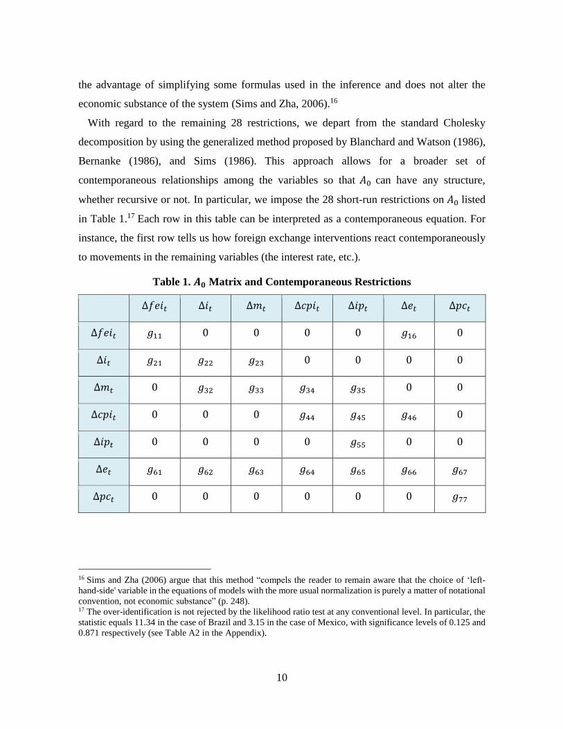
With regard to the remaining 28 restrictions, we depart from the standard Cholesky
decomposition by using the generalized method proposed by Blanchard and Watson (1986),
Bernanke (1986), and Sims (1986). This approach allows for a broader set of
contemporaneous relationships among the variables so that 𝐴0 can have any structure,
whether recursive or not. In particular, we impose the 28 short-run restrictions on 𝐴0 listed
in Table 1.17 Each row in this table can be interpreted as a contemporaneous equation. For
instance, the first row tells us how foreign exchange interventions react contemporaneously
to movements in the remaining variables (the interest rate, etc.).
Table 1. 𝑨𝟎 Matrix and Contemporaneous Restrictions
Δ𝑓𝑒𝑖𝑡 Δ𝑖𝑡 Δ𝑚𝑡 Δ𝑐𝑝𝑖𝑡 Δ𝑖𝑝𝑡 Δ𝑒𝑡 Δ𝑝𝑐𝑡
Δ𝑓𝑒𝑖𝑡 𝑔11 0 0 0 0 𝑔16 0
Δ𝑖𝑡 𝑔21 𝑔22 𝑔23 0 0 0 0
Δ𝑚𝑡 0 𝑔32 𝑔33 𝑔34 𝑔35 0 0
Δ𝑐𝑝𝑖𝑡 0 0 0 𝑔44 𝑔45 𝑔46 0
Δ𝑖𝑝𝑡 0 0 0 0 𝑔55 0 0
Δ𝑒𝑡 𝑔61 𝑔62 𝑔63 𝑔64 𝑔65 𝑔66 𝑔67
Δ𝑝𝑐𝑡 0 0 0 0 0 0 𝑔77
16 Sims and Zha (2006) argue that this method “compels the reader to remain aware that the choice of ‘left-
hand-side' variable in the equations of models with the more usual normalization is purely a matter of notational
convention, not economic substance” (p. 248). 17 The over-identification is not rejected by the likelihood ratio test at any conventional level. In particular, the
statistic equals 11.34 in the case of Brazil and 3.15 in the case of Mexico, with significance levels of 0.125 and
0.871 respectively (see Table A2 in the Appendix).
11
Note in the first row of Table 1 we assume that foreign exchange interventions react
contemporaneously solely to the exchange rate. This assumption is consistent with the
evidence provided by the leaning-against-the-wind literature and follows closely Kim (2003)
and Echavarría et al. (2009)’s approach for the cases of the US and Colombia, respectively.18
The second row introduces the contemporaneous responses of Δ𝑖𝑡 . The 𝑔21 and 𝑔23
parameters are left free to allow for the possibility that interventions are not fully sterilized
and, interestingly, to capture their contemporaneous interaction with monetary policy. The
contemporaneous response of Δ𝑖𝑡 toward output and prices is assumed to be null (𝑔24 and
𝑔25 = 0, which is based on Kim’s argument that information on output and prices is not
available within a month).19 The contemporaneous response to the exchange rate is set to 0
because both Mexico and Brazil (formally) conduct monetary policy under inflation targets.
Furthermore, in line with Echavarría et al. (2009) but in contrast with Kim (2003), 𝑔27 is
assumed to equal 0. Kim (2003) assumes otherwise in order to solve the standard “price
puzzle” that characterizes the US economy. The Appendix shows this puzzle appears only
for Brazil and, to tackle this issue, Section 4 shows that allowing for 𝑔27 to be different from
0 does not alter any of our qualitative results.
The third row in Table 2 denotes the conventional money demand equation and the fourth
and fifth rows (contemporaneously) determine price and output (see Sims and Zha (2006),
Kim (1999), Kim and Roubini (2000), Kim (2003), and Echavarría et al. (2009) for other
papers using the same money demand specification). The 𝑔41, 𝑔42, 𝑔43, 𝑔47, 𝑔51, 𝑔52, 𝑔53,
𝑔54 , 𝑔56 , and 𝑔57 parameters are set to 0 because, as argued by Kim (2003), inertia,
adjustment costs, and planning delays preclude firms from changing either prices or output
immediately in response to monetary policy and financial signals. On the other hand, we take
an agnostic approach with regard to contemporaneous “exchange rate pass-through.” That is,
we let prices contemporaneously respond to the exchange rate and thus leave the 𝑔46
parameter free. Section 4 shows that changing this assumption does not alter our qualitative
results. See Section 2 for comments about pass-through in Cortés (2013), Capistrán et al.
18 See, for instance, Adler and Tovar (2011) for a reference in this literature in which the main goal of
interventions is to stabilize the exchange rate. 19 This assumption has been widely used in the monetary literature of the business cycles. See Gordon and
Leeper (1994); Kim and Roubini (2000) and Sims and Zha (2006) for references.
12
(2012), Nogueira and León-Ledesma (2009), Barbosa-Filho (2008), Mihaljek and Klau
(2008), Nogueira (2007), and Belaisch (2003).
In the sixth row, we let the exchange rate respond contemporaneously to all of the variables.
These assumptions are in line with Echavarría et al. (2009) but contrast with Kim (2003).
Our and Echavarría et al. (2009)’s argument for the case of Colombia is that commodity
prices are more relevant in determining the local currency in developing countries than in
determining the US dollar.
Finally, in the seventh row, we assume that commodity prices are contemporaneously
exogenous. This assumption arises from the fact that the economic conditions of Brazil and
Mexico do not have such a strong impact on the IMF’s price index of commodities as the
economic conditions of the US. Brazil, for instance, is a large exporter of sugar, coffee, beef,
poultry meat, soybeans, soybean meal, and iron ore. However, these products represent only
0.16 percent of non-fuel commodities, which in turn represent only an average of 0.37 percent
for the commodity price index used in this paper. Along the same lines, Mexico produces
only a small world share of its main export commodity: crude petroleum.20
4. Results
We add a constant, 4 lags, the US federal funds rate, and a dummy variable for 2008:10-
2009:6 to the reduced-form in Equation (2) and estimate the resulting model.21
4.1. Impulse Responses to FX Intervention Shocks
Figures 3-8 and 11-18 report the responses of the endogenous variables to a one standard
deviation shock in FX interventions. The figures that appear on the right refer to the impulse
responses for Mexico and those on the left refer to Brazil. In order to facilitate the comparison
we use the same scale in all figures.
20 These data refer to the IMF’s Commodity Price Index calculated between 2004 and 2013
(http://www.imf.org/external/np/res/commod/index.aspx). 21 The dummy variable is included to account for the potential effect of the most recent financial crisis. The
resulting reduced form of the model is written as follows: 𝑦𝑡 = 𝑎 + 𝐵(𝐿)𝑦𝑡−1 + 𝐷𝑥𝑡 + 𝑑 + 𝑢𝑡 where 𝑎 is a
vector of constants, 𝐵(𝐿) is a polynomial matrix in the lag operator, 𝐷 is the matrix of coefficients associated
with the exogenous variables, 𝑥𝑡 is the vector of exogenous variables, 𝑑 is a dummy variable that equals 1 for
2008:10-2009:6, and 𝑢𝑡 is the vector of reduced form residuals.
13
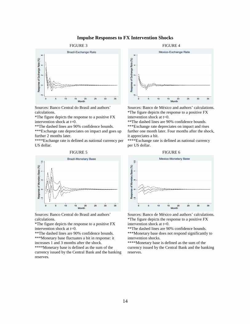
Figures 3-4 provide information on the effectiveness of FX market interventions. These
figures show that net dollar purchases are associated with a significant impact on the
exchange rate. In both Brazil and Mexico, the sign of the response is as expected since a
positive shock in FX intervention generates a depreciation of the Brazilian real and of the
peso (Figures 3 and 4, respectively). In both countries the effect is short-lived: whereas in
Mexico this effect lasts two months, in Brazil the effect lasts only one month.
Figures 5-6 refer to the reaction of monetary bases to the positive FX intervention shock.
Note that there are some fluctuations right after the shock in Brazil. However, the
contemporaneous response of the monetary base is not significant in either Mexico or Brazil.
This result, along with the evidence displayed in Figures 11-12, shows that FX interventions
are not associated with an immediate expansion in the monetary conditions (i.e. an increase
in the monetary base and a fall in the interest rate). Hence, we conclude that the interventions
are fully sterilized in both Mexico and Brazil.
Putting together Figures 3-6 allows us to link our results with the empirical literature. In
particular, the results presented in this paper are consistent with the findings that fully
sterilized interventions have significant effects on the exchange rate in the short run (see
Tapia and Tokman, 2004; Rincón and Toro, 2010; Kamil, 2008; Echavarría et al., 2010;
Echavarría et al., 2009; Kohlscheen and Andrade, 2013; Guimarães, 2004; and Section 2 for
a review of this literature). This consistency with the empirical literature provides external
validity to the identification strategy we have pursued.
14
Impulse Responses to FX Intervention Shocks
FIGURE 3 FIGURE 4
Sources: Banco Central do Brasil and authors’ Sources: Banco de México and authors’ calculations.
calculations. *The figure depicts the response to a positive FX
*The figure depicts the response to a positive FX intervention shock at t=0.
intervention shock at t=0. **The dashed lines are 90% confidence bounds.
**The dashed lines are 90% confidence bounds. ***Exchange rate depreciates on impact and rises
***Exchange rate depreciates on impact and goes up further one month later. Four months after the shock,
further 2 months later. it appreciates a bit.
****Exchange rate is defined as national currency per ****Exchange rate is defined as national currency
US dollar. per US dollar.
FIGURE 5 FIGURE 6
Sources: Banco Central do Brasil and authors’ Sources: Banco de México and authors’ calculations.
calculations. *The figure depicts the response to a positive FX
*The figure depicts the response to a positive FX intervention shock at t=0.
intervention shock at t=0. **The dashed lines are 90% confidence bounds.
**The dashed lines are 90% confidence bounds. ***Monetary base does not respond significantly to
***Monetary base fluctuates a bit in response: it intervention shocks.
increases 1 and 3 months after the shock. ****Monetary base is defined as the sum of the
****Monetary base is defined as the sum of the currency issued by the Central Bank and the banking
currency issued by the Central Bank and the banking reserves.
reserves.
15
Impulse Responses to FX Intervention Shocks (continuation)
FIGURE 7 FIGURE 8
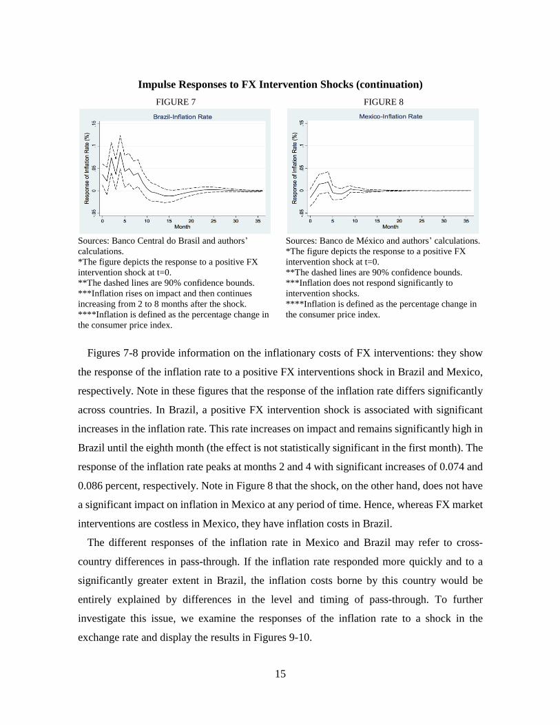
Sources: Banco Central do Brasil and authors’ Sources: Banco de México and authors’ calculations.
calculations. *The figure depicts the response to a positive FX
*The figure depicts the response to a positive FX intervention shock at t=0.
intervention shock at t=0. **The dashed lines are 90% confidence bounds.
**The dashed lines are 90% confidence bounds. ***Inflation does not respond significantly to
***Inflation rises on impact and then continues intervention shocks.
increasing from 2 to 8 months after the shock. ****Inflation is defined as the percentage change in
****Inflation is defined as the percentage change in the consumer price index.
the consumer price index.
Figures 7-8 provide information on the inflationary costs of FX interventions: they show
the response of the inflation rate to a positive FX interventions shock in Brazil and Mexico,
respectively. Note in these figures that the response of the inflation rate differs significantly
across countries. In Brazil, a positive FX intervention shock is associated with significant
increases in the inflation rate. This rate increases on impact and remains significantly high in
Brazil until the eighth month (the effect is not statistically significant in the first month). The
response of the inflation rate peaks at months 2 and 4 with significant increases of 0.074 and
0.086 percent, respectively. Note in Figure 8 that the shock, on the other hand, does not have
a significant impact on inflation in Mexico at any period of time. Hence, whereas FX market
interventions are costless in Mexico, they have inflation costs in Brazil.
The different responses of the inflation rate in Mexico and Brazil may refer to cross-
country differences in pass-through. If the inflation rate responded more quickly and to a
significantly greater extent in Brazil, the inflation costs borne by this country would be
entirely explained by differences in the level and timing of pass-through. To further
investigate this issue, we examine the responses of the inflation rate to a shock in the
exchange rate and display the results in Figures 9-10.
16
Response of Inflation Rate to Exchange Rate Shocks
FIGURE 9 FIGURE 10
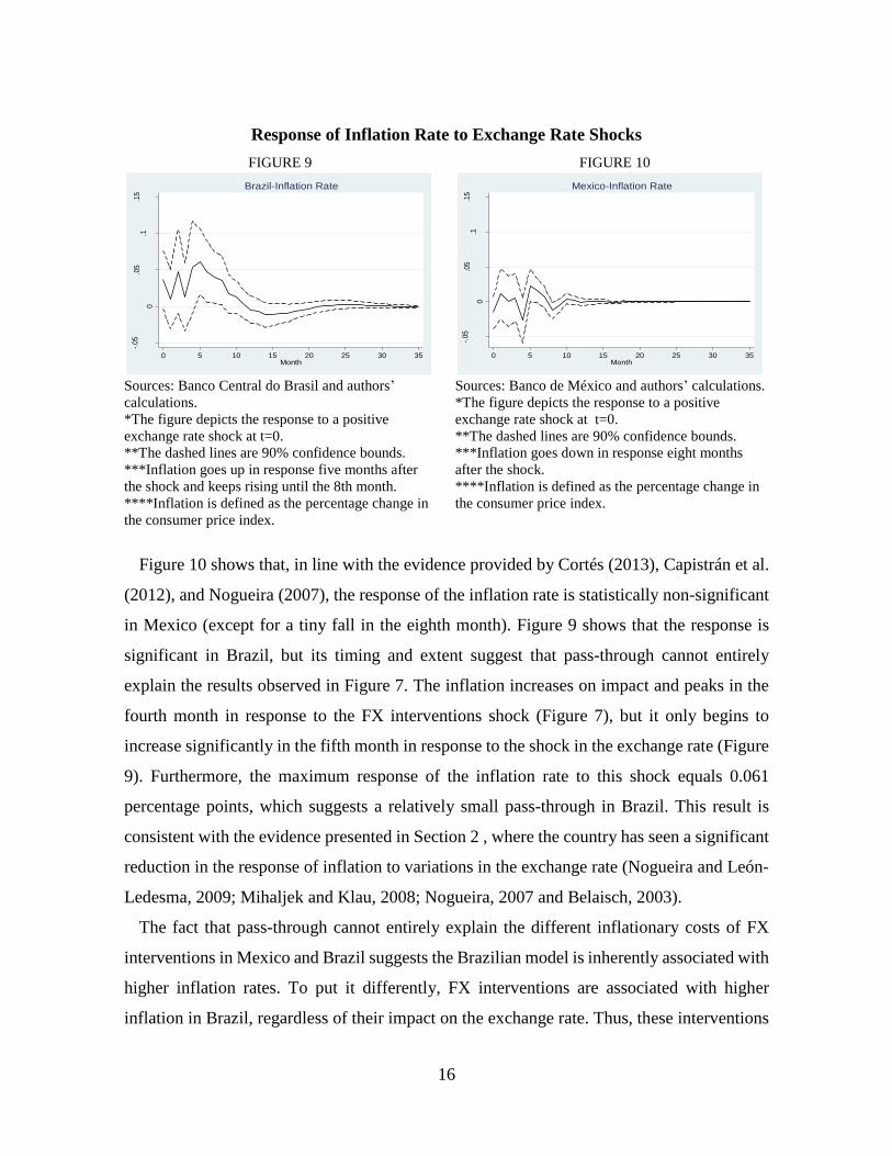
Sources: Banco Central do Brasil and authors’ Sources: Banco de México and authors’ calculations.
calculations. *The figure depicts the response to a positive
*The figure depicts the response to a positive exchange rate shock at t=0.
exchange rate shock at t=0. **The dashed lines are 90% confidence bounds.
**The dashed lines are 90% confidence bounds. ***Inflation goes down in response eight months
***Inflation goes up in response five months after after the shock.
the shock and keeps rising until the 8th month. ****Inflation is defined as the percentage change in
****Inflation is defined as the percentage change in the consumer price index.
the consumer price index.
Figure 10 shows that, in line with the evidence provided by Cortés (2013), Capistrán et al.
(2012), and Nogueira (2007), the response of the inflation rate is statistically non-significant
in Mexico (except for a tiny fall in the eighth month). Figure 9 shows that the response is
significant in Brazil, but its timing and extent suggest that pass-through cannot entirely
explain the results observed in Figure 7. The inflation increases on impact and peaks in the
fourth month in response to the FX interventions shock (Figure 7), but it only begins to
increase significantly in the fifth month in response to the shock in the exchange rate (Figure
9). Furthermore, the maximum response of the inflation rate to this shock equals 0.061
percentage points, which suggests a relatively small pass-through in Brazil. This result is
consistent with the evidence presented in Section 2 , where the country has seen a significant
reduction in the response of inflation to variations in the exchange rate (Nogueira and León-
Ledesma, 2009; Mihaljek and Klau, 2008; Nogueira, 2007 and Belaisch, 2003).
The fact that pass-through cannot entirely explain the different inflationary costs of FX
interventions in Mexico and Brazil suggests the Brazilian model is inherently associated with
higher inflation rates. To put it differently, FX interventions are associated with higher
inflation in Brazil, regardless of their impact on the exchange rate. Thus, these interventions
-.05
.05
0.1
.15
Re
spo
nse
of
Infla
tion
Ra
te (
%)
0 5 10 15 20 25 30 35Month
Brazil-Inflation Rate
0
-.05
.05
.1.1
5
Re
spo
nse
of
Infla
tion R
ate
(%
)
0 5 10 15 20 25 30 35Month
Mexico-Inflation Rate

17
must cause an inflation increase through alternative mechanisms. A probable mechanism
refers to the discretionary nature of the net dollar purchases performed by the central bank.
Because one would expect expectations on inflation to be more unstable in a discretionary
model, FX interventions may increase these expectations, thereby increasing inflation.
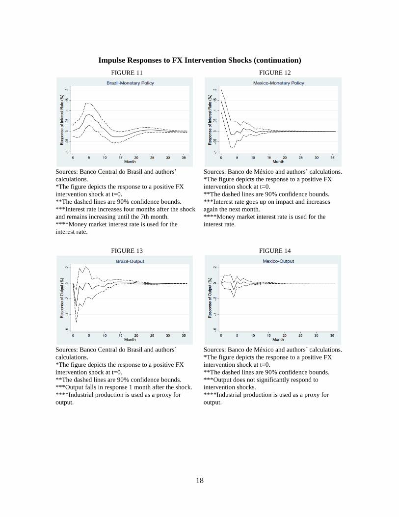
Before proceeding to the next subsection, we compare the interaction between exchange
rate and conventional monetary policies across the two FX interventions models. Figures 11
and 12 display the responses of the interest rate to the FX interventions shock in Brazil and
Mexico, respectively. Note in these figures that the nature of the interaction between the
policies is of a different nature in each country. Whereas the interest rate increases
immediately in response to the shock in Mexico, the Central Bank of Brazil raises this rate
only four months after the shock. In other words, we observe a “late” response of interest rate
setting in Brazil relative to Mexico. This result is not surprising given that the Brazilian
model entails FX interventions that are performed on a more regular basis. Because
interventions are relatively more frequent in Brazil than in Mexico, it may make it more
difficult for Brazil to raise the interest rate during each intervention. Thus, we observe in
Figure 12 a later response of the interest rate to the FX interventions shock.
The fact that interest rate setting responds later in Brazil may partially explain the results
observed in Figures 7-8. Whatever the mechanism through which the Brazilian inflation
increases is, the later response of monetary policy does not help reduce the different
responses of the inflation rate to the FX interventions shock.
18
Impulse Responses to FX Intervention Shocks (continuation)
FIGURE 11 FIGURE 12
Sources: Banco Central do Brasil and authors’ Sources: Banco de México and authors’ calculations.
calculations. *The figure depicts the response to a positive FX
*The figure depicts the response to a positive FX intervention shock at t=0.
intervention shock at t=0. **The dashed lines are 90% confidence bounds.
**The dashed lines are 90% confidence bounds. ***Interest rate goes up on impact and increases
***Interest rate increases four months after the shock again the next month.
and remains increasing until the 7th month. ****Money market interest rate is used for the
****Money market interest rate is used for the interest rate.
interest rate.
FIGURE 13 FIGURE 14
Sources: Banco Central do Brasil and authors´ Sources: Banco de México and authors´ calculations.
calculations. *The figure depicts the response to a positive FX
*The figure depicts the response to a positive FX intervention shock at t=0.
intervention shock at t=0. **The dashed lines are 90% confidence bounds.
**The dashed lines are 90% confidence bounds. ***Output does not significantly respond to
***Output falls in response 1 month after the shock. intervention shocks.
****Industrial production is used as a proxy for ****Industrial production is used as a proxy for
output. output.

19
Impulse Responses to FX Intervention Shocks (continuation)
FIGURE 15 FIGURE 16
Sources: Banco Central do Brasil and authors´ Sources: Banco de México and authors´ calculations.
calculations. *The figure depicts the response to a positive FX
*The figure depicts the response to a positive FX intervention shock at t=0.
intervention shock at t=0. **The dashed lines are 90% confidence bounds.
**The dashed lines are 90% confidence bounds. ***Commodity prices go up in response 4 months
***Commodity prices fall in response 1 month after after the shock.
the shock, and goes down further 7 months later. ***IMF´s commodity price index is used for
***IMF´s commodity price index is used for commodity prices.
commodity prices.
FIGURE 17 FIGURE 18
Sources: Banco Central do Brasil and authors´ Sources: Banco de México and authors´ calculations.
calculations. *The figure depicts the response to a positive FX
*The figure depicts the response to a positive FX intervention shock at t=0.
intervention shock at t=0. **The dashed lines are 90% confidence bounds.
**The dashed lines are 90% confidence bounds. ***Dollar purchases increase on impact and reduce
***Dollar purchases increase on impact and then in the next month.
fluctuate in the next four months.
4.2. Variance Decomposition
Tables 2-3 display the forecast error variance decomposition of inflation for Brazil and
Mexico, respectively. Each column in these tables refers to one of the seven shocks and
20
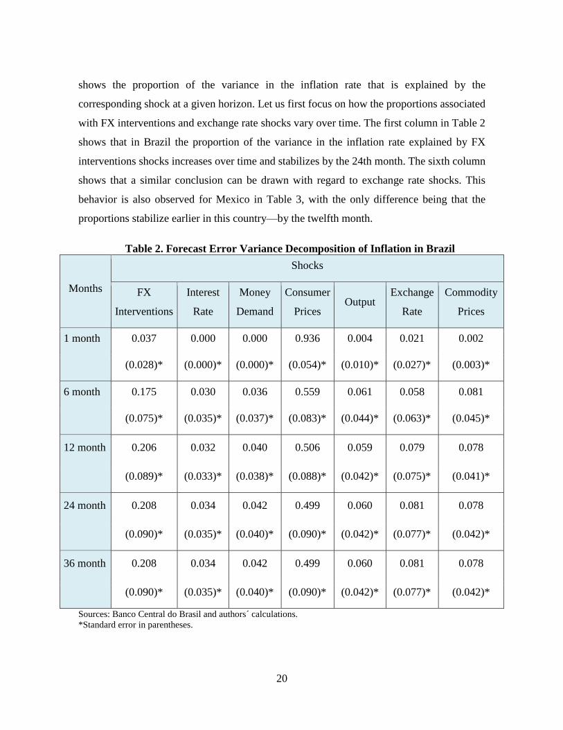
shows the proportion of the variance in the inflation rate that is explained by the
corresponding shock at a given horizon. Let us first focus on how the proportions associated
with FX interventions and exchange rate shocks vary over time. The first column in Table 2
shows that in Brazil the proportion of the variance in the inflation rate explained by FX
interventions shocks increases over time and stabilizes by the 24th month. The sixth column
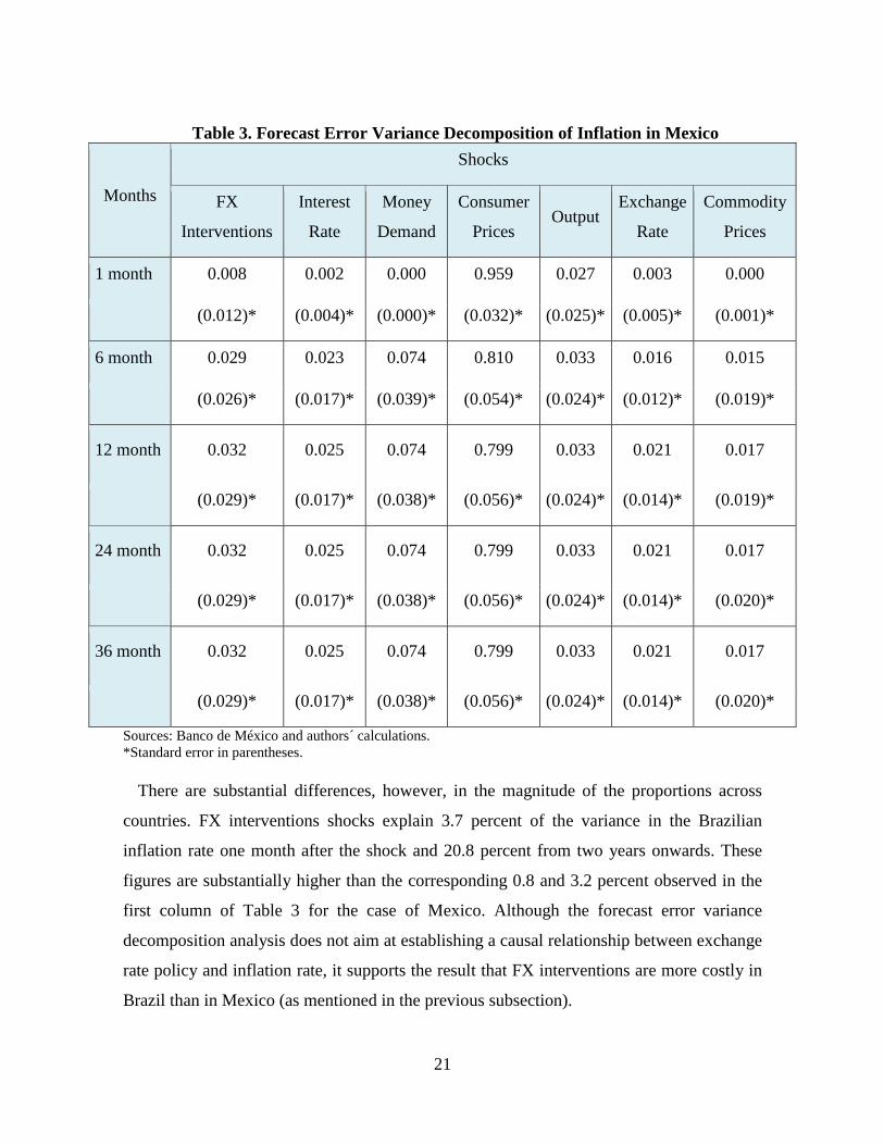
shows that a similar conclusion can be drawn with regard to exchange rate shocks. This
behavior is also observed for Mexico in Table 3, with the only difference being that the
proportions stabilize earlier in this country—by the twelfth month.
Table 2. Forecast Error Variance Decomposition of Inflation in Brazil
Months
Shocks
FX
Interventions
Interest
Rate
Money
Demand
Consumer
Prices Output
Exchange
Rate
Commodity
Prices
1 month 0.037 0.000 0.000 0.936 0.004 0.021 0.002
(0.028)* (0.000)* (0.000)* (0.054)* (0.010)* (0.027)* (0.003)*
6 month 0.175 0.030 0.036 0.559 0.061 0.058 0.081
(0.075)* (0.035)* (0.037)* (0.083)* (0.044)* (0.063)* (0.045)*
12 month 0.206 0.032 0.040 0.506 0.059 0.079 0.078
(0.089)* (0.033)* (0.038)* (0.088)* (0.042)* (0.075)* (0.041)*
24 month 0.208 0.034 0.042 0.499 0.060 0.081 0.078
(0.090)* (0.035)* (0.040)* (0.090)* (0.042)* (0.077)* (0.042)*
36 month 0.208 0.034 0.042 0.499 0.060 0.081 0.078
(0.090)* (0.035)* (0.040)* (0.090)* (0.042)* (0.077)* (0.042)*
Sources: Banco Central do Brasil and authors´ calculations.
*Standard error in parentheses.
21
Table 3. Forecast Error Variance Decomposition of Inflation in Mexico
Months
Shocks
FX
Interventions
Interest
Rate
Money
Demand
Consumer
Prices Output
Exchange
Rate
Commodity
Prices
1 month 0.008 0.002 0.000 0.959 0.027 0.003 0.000
(0.012)* (0.004)* (0.000)* (0.032)* (0.025)* (0.005)* (0.001)*
6 month 0.029 0.023 0.074 0.810 0.033 0.016 0.015
(0.026)* (0.017)* (0.039)* (0.054)* (0.024)* (0.012)* (0.019)*
12 month 0.032 0.025 0.074 0.799 0.033 0.021 0.017
(0.029)* (0.017)* (0.038)* (0.056)* (0.024)* (0.014)* (0.019)*
24 month 0.032 0.025 0.074 0.799 0.033 0.021 0.017
(0.029)* (0.017)* (0.038)* (0.056)* (0.024)* (0.014)* (0.020)*
36 month 0.032 0.025 0.074 0.799 0.033 0.021 0.017
(0.029)* (0.017)* (0.038)* (0.056)* (0.024)* (0.014)* (0.020)*
Sources: Banco de México and authors´ calculations.
*Standard error in parentheses.
There are substantial differences, however, in the magnitude of the proportions across
countries. FX interventions shocks explain 3.7 percent of the variance in the Brazilian
inflation rate one month after the shock and 20.8 percent from two years onwards. These
figures are substantially higher than the corresponding 0.8 and 3.2 percent observed in the
first column of Table 3 for the case of Mexico. Although the forecast error variance
decomposition analysis does not aim at establishing a causal relationship between exchange
rate policy and inflation rate, it supports the result that FX interventions are more costly in
Brazil than in Mexico (as mentioned in the previous subsection).
22
As for the proportions explained by shocks in the exchange rate, the figures are notably
small in both countries. For Brazil, these proportions equal 2.1 and 8.1 percent at 1 and at 24
months, respectively. For Mexico, the proportions equal 0.3 and 2.1. These numbers support
the idea that the level of pass-through is small in both economies.
Certainly, the level of pass-through is greater for Brazil than it is for Mexico in absolute
terms. However, the proportion explained by exchange rate shocks is smaller relative to the
corresponding proportion associated with FX interventions shocks for the case of Brazil. For
instance, the difference between the figures that appear in the sixth and first columns equals
1.6 and 12.7 percent at 1 and 24 months for Brazil and 0.5 and 1.1 percent for Mexico. This
result supports the result that differences in the level of pass-through cannot entirely explain
the fact that FX interventions have higher inflationary costs in Brazil than in Mexico.
5. Robustness
This subsection examines the robustness of our results by changing identifying restrictions.
We focus on two cases: the contemporaneous response of the interest rate to commodity
prices and the response of consumer prices to the exchange rate (concerning the 𝑔27 and 𝑔46
parameters, respectively). Three reasons motivate this analysis. First, by imposing these
restrictions, our model departs from either Kim’s (2003) setup and/or Echavarría et al.’s
(2009) approach. Second, the restriction on 𝑔27 is connected to the empirical finding that
some economies present a “price puzzle,” i.e. prices do not always respond in the expected
direction to conventional monetary policy. This finding is relevant to our study because the
original set of contemporaneous restrictions we have imposed generates a “price puzzle” for
the case of Brazil.22 Third, the restriction on 𝑔46 is connected to contemporaneous pass-
through and, therefore, is at the core of our main results.
22 The result that inflation increases in response to a monetary policy tightening in Brazil comes from at least
two main sources. First, this response might be part of a more general problem identified in the SVAR literature,
according to which the forward-looking nature of central banks may not be fully captured: given that that central
banks react in advance to inflationary pressures, SVAR models that do not include information about
prospective pressures may be unable to identify “true” monetary policy shocks. To solve for this so-called “price
puzzle”, some authors include commodity prices in the VAR estimations under the argument that these prices
reflect inflationary pressures that are not incorporated in other variables (Sims, 1992; Christiano et al., 1999;
Kim, 1999, 2003 and Sims and Zha, 2006). The present paper shows the result of this exercise in the appendix.
23
The review of the two identifying restrictions yields the three alternative models that are
described by the following conditions: 𝑔27 ≠ 0; 𝑔46 = 0; and 𝑔46 = 0 and 𝑔27 ≠ 0. For the
sake of brevity, we present solely the response of ∆𝑐𝑝𝑖𝑡 to a shock in ∆𝑖𝑡 for the first case
and the responses of ∆𝑐𝑝𝑖𝑡 and ∆𝑖𝑡 to the FX interventions shock for the three cases.
Presenting these responses allows us to show that the “price puzzle” disappears when 𝑔27 ≠
0 and to examine the robustness of the model to changes in the two identifying restrictions.
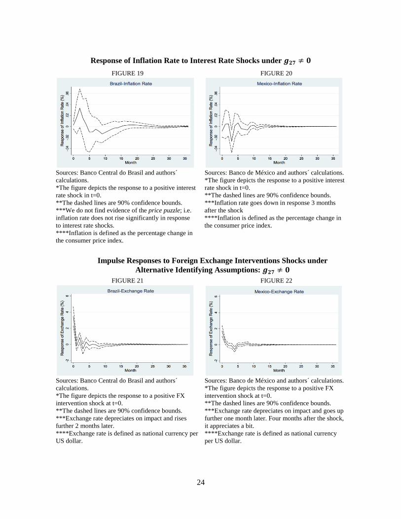
Figures 19-38 show the responses for the three alternative models.
Note in Figure 19 that when 𝑔27 ≠ 0, the “price puzzle” disappears in Brazil; thus a rise in
the interest rate is not associated with an increase in the inflation rate.23 In both this model
and in the remaining two setups, the consideration of alternative identifying restrictions
modifies neither the qualitative results nor the significance of the responses. In particular, in
the three alternatives we observe that (i) FX interventions are effective in both countries and
their effects on the exchange rate are short-lived; (ii) the inflation rises in response to the
shock in Brazil but does not respond significantly in Mexico; and (iii) the central bank
increases the interest rate immediately after the shock in Mexico but it does not do that in
Brazil.
Second, the unexpected response of inflation rates to monetary policy may also be due to idiosyncratic features
of the Brazilian economy. As discussed below, the fact that Brazil intervenes frequently in the FX market is
likely to introduce noise in the relationship between the interest rate and inflation. This fact may make it more
difficult to raise the interest rate during each intervention to offset inflationary pressures. 23 However, leaving 𝑔27 free does not solve completely the puzzle; we do not observe a fall in the inflation rate
in response to a contractionary monetary policy shock as would be predicted by standard economic theory.
24
Response of Inflation Rate to Interest Rate Shocks under 𝒈𝟐𝟕 ≠ 𝟎
FIGURE 19 FIGURE 20
Sources: Banco Central do Brasil and authors´ Sources: Banco de México and authors´ calculations.
calculations. *The figure depicts the response to a positive interest
*The figure depicts the response to a positive interest rate shock in t=0.
rate shock in t=0. **The dashed lines are 90% confidence bounds.
**The dashed lines are 90% confidence bounds. ***Inflation rate goes down in response 3 months
***We do not find evidence of the price puzzle; i.e. after the shock
inflation rate does not rise significantly in response ****Inflation is defined as the percentage change in
to interest rate shocks. the consumer price index.
****Inflation is defined as the percentage change in
the consumer price index.
Impulse Responses to Foreign Exchange Interventions Shocks under
Alternative Identifying Assumptions: 𝒈𝟐𝟕 ≠ 𝟎
FIGURE 21 FIGURE 22
Sources: Banco Central do Brasil and authors´ Sources: Banco de México and authors´ calculations.
calculations. *The figure depicts the response to a positive FX
*The figure depicts the response to a positive FX intervention shock at t=0.
intervention shock at t=0. **The dashed lines are 90% confidence bounds.
**The dashed lines are 90% confidence bounds. ***Exchange rate depreciates on impact and goes up
***Exchange rate depreciates on impact and rises further one month later. Four months after the shock,
further 2 months later. it appreciates a bit.
****Exchange rate is defined as national currency per ****Exchange rate is defined as national currency
US dollar. per US dollar.
25
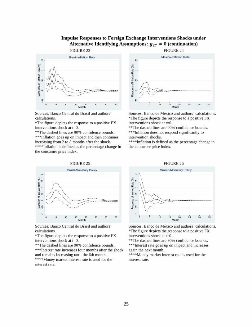
Impulse Responses to Foreign Exchange Interventions Shocks under
Alternative Identifying Assumptions: 𝒈𝟐𝟕 ≠ 𝟎 (continuation)
FIGURE 23 FIGURE 24
Sources: Banco Central do Brasil and authors´ Sources: Banco de México and authors´ calculations.
calculations. *The figure depicts the response to a positive FX
*The figure depicts the response to a positive FX interventions shock at t=0.
interventions shock at t=0. **The dashed lines are 90% confidence bounds.
**The dashed lines are 90% confidence bounds. ***Inflation does not respond significantly to
***Inflation goes up on impact and then continues intervention shocks.
increasing from 2 to 8 months after the shock. ****Inflation is defined as the percentage change in
****Inflation is defined as the percentage change in the consumer price index.
the consumer price index.
FIGURE 25 FIGURE 26
Sources: Banco Central do Brasil and authors´ Sources: Banco de México and authors´ calculations.
calculations. *The figure depicts the response to a positive FX
*The figure depicts the response to a positive FX interventions shock at t=0.
interventions shock at t=0. **The dashed lines are 90% confidence bounds.
**The dashed lines are 90% confidence bounds. ***Interest rate goes up on impact and increases
***Interest rate increases four months after the shock again the next month.
and remains increasing until the 6th month. ****Money market interest rate is used for the
****Money market interest rate is used for the interest rate.
interest rate.
26
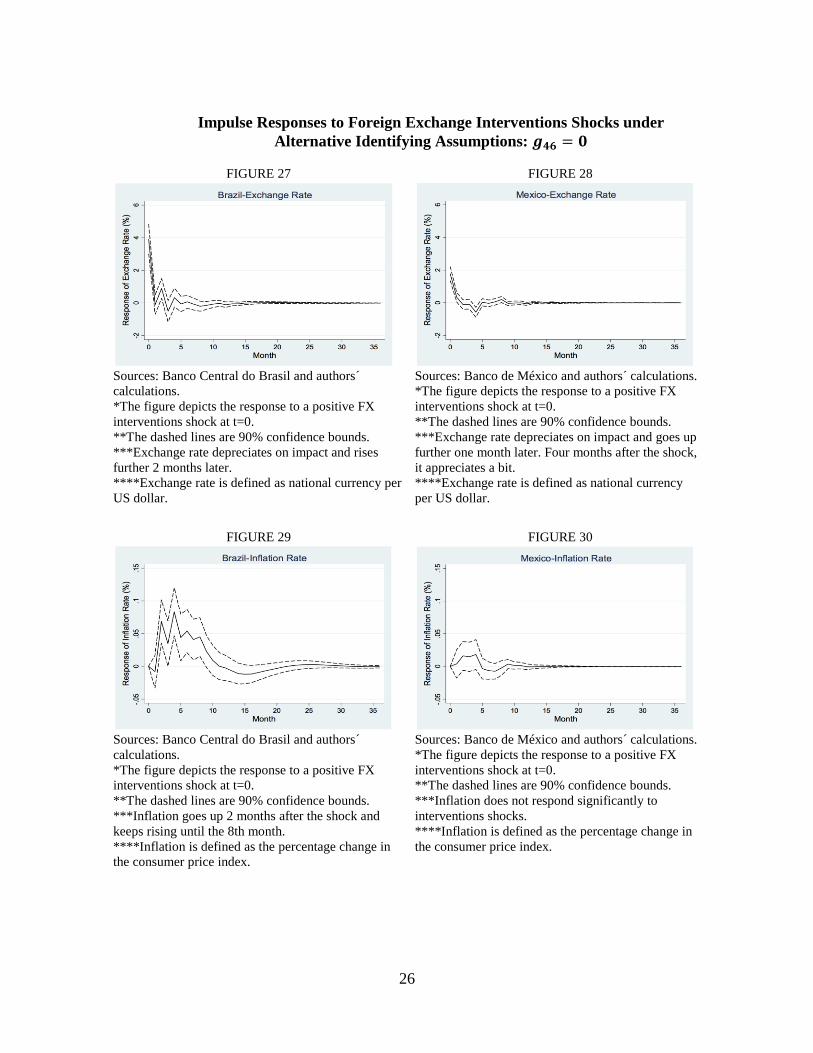
Impulse Responses to Foreign Exchange Interventions Shocks under
Alternative Identifying Assumptions: 𝒈𝟒𝟔 = 𝟎
FIGURE 27 FIGURE 28
Sources: Banco Central do Brasil and authors´ Sources: Banco de México and authors´ calculations.
calculations. *The figure depicts the response to a positive FX
*The figure depicts the response to a positive FX interventions shock at t=0.
interventions shock at t=0. **The dashed lines are 90% confidence bounds.
**The dashed lines are 90% confidence bounds. ***Exchange rate depreciates on impact and goes up
***Exchange rate depreciates on impact and rises further one month later. Four months after the shock,
further 2 months later. it appreciates a bit.
****Exchange rate is defined as national currency per ****Exchange rate is defined as national currency
US dollar. per US dollar.
FIGURE 29 FIGURE 30
Sources: Banco Central do Brasil and authors´ Sources: Banco de México and authors´ calculations.
calculations. *The figure depicts the response to a positive FX
*The figure depicts the response to a positive FX interventions shock at t=0.
interventions shock at t=0. **The dashed lines are 90% confidence bounds.
**The dashed lines are 90% confidence bounds. ***Inflation does not respond significantly to
***Inflation goes up 2 months after the shock and interventions shocks.
keeps rising until the 8th month. ****Inflation is defined as the percentage change in
****Inflation is defined as the percentage change in the consumer price index.
the consumer price index.
27
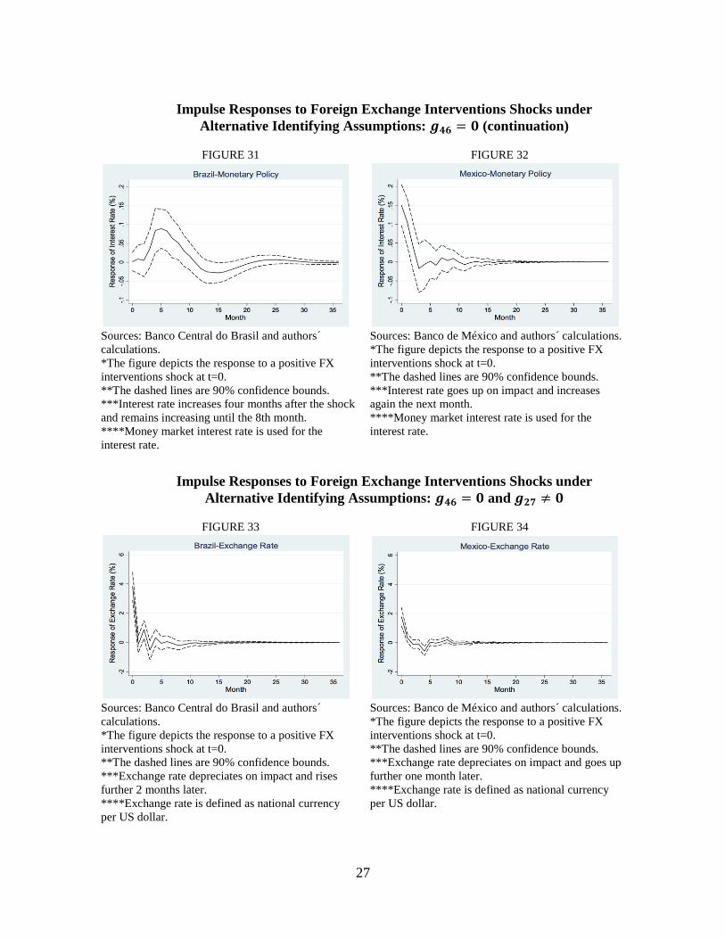
Impulse Responses to Foreign Exchange Interventions Shocks under
Alternative Identifying Assumptions: 𝒈𝟒𝟔 = 𝟎 (continuation)
FIGURE 31 FIGURE 32
Sources: Banco Central do Brasil and authors´ Sources: Banco de México and authors´ calculations.
calculations. *The figure depicts the response to a positive FX
*The figure depicts the response to a positive FX interventions shock at t=0.
interventions shock at t=0. **The dashed lines are 90% confidence bounds.
**The dashed lines are 90% confidence bounds. ***Interest rate goes up on impact and increases
***Interest rate increases four months after the shock again the next month.
and remains increasing until the 8th month. ****Money market interest rate is used for the
****Money market interest rate is used for the interest rate.
interest rate.
Impulse Responses to Foreign Exchange Interventions Shocks under
Alternative Identifying Assumptions: 𝒈𝟒𝟔 = 𝟎 and 𝒈𝟐𝟕 ≠ 𝟎
FIGURE 33 FIGURE 34
Sources: Banco Central do Brasil and authors´ Sources: Banco de México and authors´ calculations.
calculations. *The figure depicts the response to a positive FX
*The figure depicts the response to a positive FX interventions shock at t=0.
interventions shock at t=0. **The dashed lines are 90% confidence bounds.
**The dashed lines are 90% confidence bounds. ***Exchange rate depreciates on impact and goes up
***Exchange rate depreciates on impact and rises further one month later.
further 2 months later. ****Exchange rate is defined as national currency
****Exchange rate is defined as national currency per US dollar.
per US dollar.

28
Impulse Responses to Foreign Exchange Interventions Shocks under
Alternative Identifying Assumptions: 𝒈𝟒𝟔 = 𝟎 and 𝒈𝟐𝟕 ≠ 𝟎 (continuation)
FIGURE 35 FIGURE 36
Sources: Banco Central do Brasil and authors´ Sources: Banco de México and authors´ calculations.
calculations. *The figure depicts the response to a positive FX
*The figure depicts the response to a positive FX interventions shock at t=0.
interventions shock at t=0. **The dashed lines are 90% confidence bounds.
**The dashed lines are 90% confidence bounds. ***Inflation does not respond significantly to
***Inflation goes up 2 months after the shock and interventions shocks.
keeps rising until the 8th month. ****Inflation is defined as the percentage change in
****Inflation is defined as the percentage change in the consumer price index.
the consumer price index.
FIGURE 37 FIGURE 38
Sources: Banco Central do Brasil and authors´ Sources: Banco de México and authors´ calculations.
calculations. *The figure depicts the response to a positive FX
*The figure depicts the response to a positive FX interventions shock at t=0.
interventions shock at t=0. **The dashed lines are 90% confidence bounds.
**The dashed lines are 90% confidence bounds. ***Interest rate goes up on impact and increases
***Interest rate increases four months after the shock again the next month.
and remains increasing until the 8th month. ****Money market interest rate is used for the
****Money market interest rate is used for the interest rate.
interest rate.
29
6. Conclusions
This paper has provided evidence of three major results. First, FX interventions have been
successful in having a short-run impact on the exchange rate in both Mexico and Brazil. This
outcome is consistent with an existing literature that investigates the effects of FX
interventions in Latin-America. Second, we have found that different FX intervention models
generates differential inflationary costs, with the costs being higher in a model that involves
interventions that are discretionary and of a higher-frequency. Third, the evidence suggests
that this second result cannot not be entirely driven by cross-country differences in the level
of exchange rate pass-through.
Indeed, the higher inflationary costs associated with the Brazilian model seem to be at least
partially associated with the implicit interaction between FX interventions and interest rate
setting (conventional monetary policy). In particular, adopting a model that entails
interventions on a regular basis seems to make it more difficult to compensate them with
increases in the interest rate. That is, this intervention model makes the relationship between
interest rates and inflation significantly noisier.
30
7. References
Adler, G. and C. E. Tovar (2011). Foreign Exchange Intervention: A Shield against
Appreciation Winds? IMF Working Paper, WP/11/165, International Monetary Fund.
Barbosa-Filho, N. (2008). Inflation Targeting in Brazil: 1999-2006. International Review of
Applied Economics, 22(2), pp. 187-200.
Belaisch, A. (2003). Exchange Rate Pass-through in Brazil. IMF Working Paper, WP/3/141,
International Monetary Fund.
Bernanke, B. S. (1986). Alternative Explanations of the Money-Income Correlation.
Carnegie-Rochester Conference Series on Public Policy, 25(1), pp. 49-99.
Blanchard, O. J. and M. W. Watson (1986). Are Business Cycles all Alike? in Robert J.
Gordon (ed.), The American Business Cycle: Continuity and Change, University of
Chicago Press, pp. 123-180.
Broto, C. (2013). The Effectiveness of Forex Interventions in Four Latin American
Countries. Emerging Markets Review, 17, pp. 224-240.
Capistrán, C., R. Ibarra and M. Ramos-Francia (2012). El Traspaso de Movimientos del Tipo
de Cambio a los Precios. Un Análisis para la Economía Mexicana. El Trimestre
Económico, 79 (4), pp. 813-838.
Christiano, L. J., M. Eichenbaum and C. L. Evans (1999). Monetary Policy Shocks: What
Have We Learned and to What End? Handbook of macroeconomics, 1, 65-148.
Cortés Espada, J. F. (2013). Estimación del Traspaso del Tipo de Cambio a los Precios en
México. Monetaria, 35(2), pp. 311-344.
Cushman, D. O. and T. Zha (1997). Identifying Monetary Policy in a Small Open Economy
under Flexible Exchange Rates. Journal of Monetary Economics, 39(3), pp. 433-448.
Domaç, I. and A. Mendoza (2004). Is there Room for Foreign Exchange Interventions under
an Inflation Targeting Framework? Evidence from Mexico and Turkey. World Bank Policy
Research Working Paper, 3288, World Bank.
Echavarría, J. J., E. López and M. Misas (2009). Intervenciones Cambiarias y Política
Monetaria en Colombia. Un Análisis de VAR Estructural. Borradores de Economía, 580,
Banco de la República.
Echavarría, J. J., D. Vásquez, and M. Villamizar (2010). Impacto de las Intervenciones
Cambiarias sobre el Nivel y la Volatilidad de la Tasa de Cambio en Colombia. Ensayos
Sobre Política Económica, 28(62), pp. 12-69.
Fackler, J. S. and W. D. McMillin (1998). Historical Decomposition of Aggregate Demand
and Supply Shocks in a Small Macro Model. Southern Economic Journal, 64(3), pp. 648-
664.
Faust, J. and E. M. Leeper (1997). When Do Long-Run Identifying Restrictions Give
Reliable Results? Journal of Business and Economic Statistics, 15(3), pp. 345-353.
31
García-Verdú, S. and M. Ramos-Francia (2014). Interventions and Expected Exchange Rates
in Emerging Market Economies. The Quarterly Journal of Finance, 4(01), 1450002.
García-Verdú, S. and M. Zerecero (2014). On Central Bank Interventions in the
Mexican Peso/Dollar Foreign Exchange Market. Banco de México Working Papers, 2014-
19, Banco de México.
Gordon, D. B. and E. M. Leeper (1994). The Dynamic Impacts of Monetary Policy: An
Exercise in Tentative Identification. Journal of Political Economy, 102(6), pp. 1228-1247.
Guimarães, R. F. (2004). Foreign Exchange Intervention and Monetary Policy in Japan:
Evidence from Identified VARs. Money, Macro, and Finance (MMF) Research Group
Conference 2004-8, Cass Business School, London.
International Monetary Fund (Ed.) (2015), Annual Report on Exchange Arrangements and
Exchange Restrictions, 2005. International Monetary Fund.
Ilzetzki, E., C. Reinhart and K. Rogoff (2008). Exchange Rate Arrangements entering the
21st Century: Which Anchor will Hold? University of Maryland and Harvard University.
Kamil, H. (2008). Is Central Bank Intervention Effective under Inflation Targeting Regimes?
The Case of Colombia. IMF Working Papers, WP/08/88, International Monetary Fund.
Kim, S. (1999). Do Monetary Policy Shocks Matter in the G-7 Countries? Using Common
Identifying Assumptions about Monetary Policy across Countries. Journal of International
Economics, 48(2), pp. 387-412.
Kim, S. (2003). Monetary Policy, Foreign Exchange Intervention, and the Exchange Rate in
a Unifying Framework. Journal of International Economics, 60(2), pp. 355-386.
Kim, S. and N. Roubini (2000). Exchange Rate Anomalies in the Industrial Countries: A
Solution with a Structural VAR Approach. Journal of Monetary Economics, 45(3), pp.
561-586.
Kohlscheen, E. and S. C. Andrade (2013). Official Interventions through
Derivatives: Affecting the Demand for Foreign Exchange. Banco Central do Brasil
Working Papers, 317, Banco Central do Brasil.
Lastrapes, W. D. and G. Selgin (1995). The Liquidity Effect: Identifying Short-Run Interest
Rate Dynamics using Long-Run Restrictions. Journal of Macroeconomics, 17(3), pp. 387-
404.
Lütkepohl, H. (2005), New Introduction to Multiple Time Series Analysis, Springer-Verlag,
Germany, 764 pages.
McMillin, W. D. (2001). The Effects of Monetary Policy Shocks: Comparing
Contemporaneous versus Long-Run Identifying Restrictions. Southern Economic Journal,
67(3), pp. 618-636.
Menkhoff, L. (2013). Foreign Exchange Intervention in Emerging Markets: A Survey of
Empirical Studies. World Economy, 36(9), pp. 1187-1208.
32
Mihaljek, D. and M. Klau (2008). Exchange Rate Pass-through in Emerging Market
Economies: What Has Changed and Why? in Bank for International Settlements (ed.),
Transmission Mechanisms for Monetary Policy in Emerging Market Economies, BIS
Papers Series, 35, pages 103-130, Bank for International Settlements.
Neely, C. J. (2005). An Analysis of Recent Studies of the Effect of Foreign Exchange
Intervention. Federal Reserve Bank of St. Louis Review, 87(6), pp. 685-717.
Nogueira, R. P. Jr. (2007). Inflation Targeting and Exchange Rate Pass-through. Economia
Aplicada, 11(2), pp. 189-208.
Nogueira, R. P. Jr. and M. Leon-Ledesma (2009). Fear of Floating in Brazil: Did Inflation
Targeting Matter? North American Journal of Economics and Finance, 20(3), pp. 255-
266.
Rincón, H. and J. Toro (2010). Are Capital Controls and Central Bank Intervention Effective?
Borradores de Economía, 625, Banco de la República.
Sarno, L. and M. P. Taylor. (2001). Official Intervention in the Foreign Exchange Market: Is
it Effective and, if so, How Does It Work? Journal of Economic Literature, 39(3), pp. 839-
868.
Sims, C. A. (1986). Are Forecasting Models Usable for Policy Analysis? Federal Reserve
Bank of Minneapolis Quarterly Review, 10(1), pp. 2-16.
Sims, C. A. (1992). Interpreting the Macroeconomic Time Series Facts: The Effects of
Monetary Policy. European Economic Review, 36(5), 975-1000.
Sims, C. A. and T. Zha (2006). Does Monetary Policy Generate Recessions? Macroeconomic
Dynamics, 10(2), pp. 231-272.
Stone, M. R., W. C. Walker and Y. Yasui (2009). From Lombard Street to Avenida Paulista:
Foreign Exchange Liquidity Easing in Brazil in Response to the Global Shock of 2008–
09. IMF Working Papers, WP/09/259, International Monetary Fund.
Tapia, M. and A. Tokman (2004). Effects of Foreign Exchange Intervention under Public
Information: The Chilean Case. Economía: Journal of the Latin American and Caribbean
Economic Association, 4(2), pp. 215-256.
Tobal, M. (2013). Currency Mismatch: New Database and Indicators for Latin America and
the Caribbean. CEMLA Research Papers, 12, available at
http://www.cemla.org/PDF/investigacion/inv-2013-11-12.pdf.
33
Appendix Section
Table A1. Unit Root Test Statistics
Variable
Augmented Dickey-Fuller Phillips-Perron
Brazil Mexico 95% Critical
value Brazil Mexico
95% Critical
value
A. In Levels
𝑓𝑒𝑖 -3.57** -2.46** -1.94 -4.91** -3.01** -1.94
𝑖 -3.31* -3.53** -3.44 -2.78* -3.01* -3.44
𝑚 -1.47* -1.40* -3.44 -5.25** -2.06* -3.44
𝑐𝑝𝑖 -2.02* -1.40* -3.44 -1.52* -4.17** -3.44
𝑖𝑝 -2.78* -2.41* -3.44 -2.50* -2.18* -3.44
𝑒 -2.26* -3.38* -3.44 -2.37* -3.24* -3.44
𝑝𝑐 -3.25* -3.25* -3.44 -2.68* -2.68* -3.44
B. In First Differences
∆𝑓𝑒𝑖 ---- ---- ---- ---- ---- ----
∆𝑖 -5.11** -4.08** -1.94 -4.18** -10.81** -1.94
∆𝑚 -3.90** -7.57** -2.88 -21.72** -19.90** -2.88
∆𝑐𝑝𝑖 -5.79** -3.75** -2.88 -5.83** -9.72** -2.88
∆𝑖𝑝 -11.77** -4.88** -2.88 -11.73** -15.03** -2.88
∆𝑒 -8.41** -11.54** -1.94 -8.40** -11.54** -1.94
∆𝑝𝑐 -4.37** -4.37** -1.94 -8.84** -8.84** -1.94
Sources: Banco Central do Brasil, Banco de México, and authors´ calculations.
Notes: The tests for variables in levels (panel A) include a constant and a liner trend, except for 𝑓𝑒𝑖. The tests
for ∆𝑚, ∆𝑐𝑝𝑖 and ∆𝑖𝑝 (in panel B) include only a constant, and for 𝑓𝑒𝑖 (in panel A), ∆𝑖, ∆𝑒, ∆𝑝𝑐 (in panel B)
include neither a constant nor a liner trend. The lag lengths were chosen based on the AIC.
*The null hypothesis of a unit root cannot be rejected at 95% confidence level.
**The null hypothesis of a unit root is rejected at 95% percent confidence level.
34
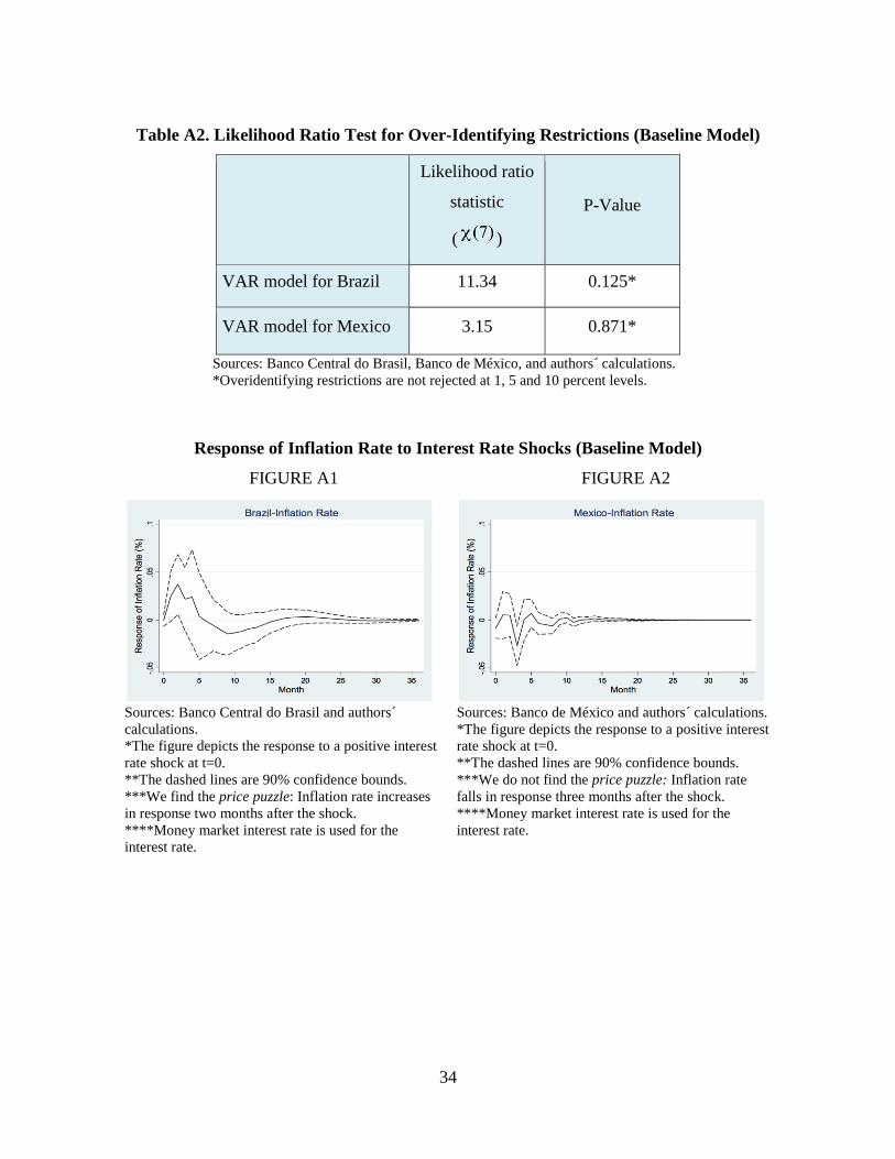
Table A2. Likelihood Ratio Test for Over-Identifying Restrictions (Baseline Model)
Likelihood ratio
statistic
( )
P-Value
VAR model for Brazil 11.34 0.125*
VAR model for Mexico 3.15 0.871*
Sources: Banco Central do Brasil, Banco de México, and authors´ calculations.
*Overidentifying restrictions are not rejected at 1, 5 and 10 percent levels.
Response of Inflation Rate to Interest Rate Shocks (Baseline Model)
FIGURE A1 FIGURE A2
Sources: Banco Central do Brasil and authors´ Sources: Banco de México and authors´ calculations.
calculations. *The figure depicts the response to a positive interest
*The figure depicts the response to a positive interest rate shock at t=0.
rate shock at t=0. **The dashed lines are 90% confidence bounds.
**The dashed lines are 90% confidence bounds. ***We do not find the price puzzle: Inflation rate
***We find the price puzzle: Inflation rate increases falls in response three months after the shock.
in response two months after the shock. ****Money market interest rate is used for the
****Money market interest rate is used for the interest rate.
interest rate.