Journal of Computational Physics167,177–195 (2001)

doi:10.1006/jcph.2000.6666, available online at http://www.idealibrary.com on

Two-Dimensional Riemann Solver for EulerEquations of Gas Dynamics

M. Brio,∗ A. R. Zakharian,† and G. M. Webb‡∗Department of Mathematics,†ACMS, Department of Mathematics, University of Arizona,

and‡Lunar and Planetary Laboratory, University of Arizona, Tucson, Arizona 85721E-mail: brio@math.arizona.edu, armis@acms.arizona.edu, cosray@lpl.arizona.edu

Received June 15, 1999; revised February 22, 2000

We construct a Riemann solver based on two-dimensional linear wave contri-butions to the numerical flux that generalizes the one-dimensional method due toRoe (1981,J. Comput. Phys.43, 157). The solver is based on a multistate Riemannproblem and is suitable for arbitrary triangular grids or any other finite volume tes-sellations of the plane. We present numerical examples illustrating the performanceof the method using both first- and second-order-accurate numerical solutions. Thenumerical flux contributions are due to one-dimensional waves and multidimensionalwaves originating from the corners of the computational cell. Under appropriate CFLrestrictions, the contributions of one-dimensional waves dominate the flux, whichexplains good performance of dimensionally split solvers in practice. The multidi-mensional flux corrections increase the accuracy and stability, allowing a larger timestep. The improvements are more pronounced on a coarse mesh and for large CFLnumbers. For the second-order method, the improvements can be comparable to theimprovements resulting from a less diffusive limiter.c© 2001 Academic Press

Key Words:Godunov-type schemes; conservation laws; two-dimensional Riemannproblem.

1. INTRODUCTION

In the past decade there have been numerous investigations of the use of linear solversto account for the multidimensional nature of hyperbolic problems. The main advantagesof such methods are an improved stability, resolution properties, and preservation of thedirectionally unsplit nature of the schemes [4, 11]. In particular, the adaptations of one-dimensional solvers in preferred directions were studied in [5, 12, 16–18]. The use ofLax–Wendroff type construction to include the cross derivative terms, which are in turndiscretized by using a one-dimensional solver, was done by LeVeque [11]. Collela [4] usedthe corner transport upwinding method based on the predictor–corrector time integration in

177

0021-9991/01 $35.00Copyright c© 2001 by Academic Press

All rights of reproduction in any form reserved.

178 BRIO, ZAKHARIAN, AND WEBB

which predictor and corrector steps use different coordinate directions. Theoretical studiesof two-dimensional Riemann problems for both scalar equations and Euler’s equations werecarried out in [3, 13, 20]. Genuine two-dimensional solvers were considered in [1] using theself-similar form of Euler’s equations, leading to a mixed hyperbolic–elliptic problem. In[8] the formulas were derived for the linear 2-D Riemann problem for a subsonic case of gasdynamics and rectangular initial conditions. The Method of Transport that does not use aRiemann problem was introduced in [6, 7]. It relies on the assumption that flux contributionsof separate waves can be decoupled and uses multidimensional waves transported frominfinitely many propagation directions.

Our motivation to use a multistate Riemann problem came from previous studies of theweak shock reflection problem, a problem that may be interpreted as a multistate Riemannproblem [2, 10].

In this paper, we construct a Riemann solver based on two-dimensional linear wavecontributions to the numerical flux. The resulting numerical flux can be viewed as a one-dimensional flux normal to the cell boundaries plus the correction terms resulting from thewaves emanating from the corners, which are computed using a multistate linear Riemannsolver. The formulas generalize results obtained in [8] for arbitrary angles and for all thewaves.

For small CFL numbers the contributions of one-dimensional waves dominate the flux,which explains a good performance of direction-split solvers in practice. The multidimen-sional flux corrections increase the stability, allowing large time steps and accuracy, althoughthe improvements are often marginal. The overall efficiency may increase or decrease de-pending on the problem, on grids, and on the choice of the multidimensional method.

In the following section, the finite volume formulation on a hexagonal and rectangulargrid is discussed. A detailed construction of the two-dimensional linear Riemann solveris described for the Euler equations of gas dynamics in Section 3. Numerical examplesillustrating the performance of the method, including a second-order-accurate version onregular rectangular as well as hexagonal Delaunay–Voronoi dual meshes, are presented inSection 4.

In the Appendix we derive the analytical solution to a multistate linear Riemann problemfor the Euler equations of gas dynamics.

2. THE FINITE VOLUME FLUX COMPUTATION

In this section we describe the use of the linear multistate Riemann solver in the simplecase involving three-state initial data in a cell-centered finite volume method on a hexagonalgrid. An example of such a grid, a regular Delaunay–Voronoi dual mesh, is shown in Fig. 1.Consider an integral form of a system of hyperbolic conservation laws

d

dt

∫A

u dS+∫0

f · n dl = 0, (1)

whereu is one of the conserved variables,A and0 represent the volume and the boundaryof the control region, andn is the outward normal to the cell. Integrating in time and overthe computational cell, shown in Fig. 1, gives the finite volume approximation,

un+1i j = un

i j −1

A

∑k

∫ 1t

0dt∫0k

f · n dl, (2)

MULTIDIMENSIONAL RIEMANN SOLVER 179

FIG. 1. Control volume of a dual Delaunay–Voronoi hexagonal mesh.

whereuni j represents the cell average at timetn and0k is the length of the edge of the compu-

tational cell. The cell averages are assumed to be given, while the fluxes are approximatedusing the values on the edge computed as solutions to the 3- and 2-state linear Riemannproblems.

The initial data needed to determine the values of the flux densityf along one of the edgesconsist of four states, as shown in Fig. 2.

The circles in this figure represent positions of the sonic wave fronts based on the aver-age sound speed of the three surrounding states. The centers of the sonic circles are shiftedby the position vector−u1t to account for the advection with average velocityu. Thus,the numerical flux across the sections of the edge, denoted bye1, e3, results from multidi-mensional waves originating from the corners of the computational cell. These fluxes areapproximated using solutions to the 3-state linear Riemann problems described in the Ap-pendix. For example, in Fig. 2, the flux across the sectione1 is computed asf(u∗(x, y, t)),whereu∗(x, y, t) is the solution of the 3-state Riemann problem with the initial data fromthe cellsO1, O2, andO3. The flux across the sectione2 is determined only by the statesO2 andO3 and can be computed using a 1-D Riemann solver. The resulting numerical flux

FIG. 2. Flux computation using three-state Riemann problems.

180 BRIO, ZAKHARIAN, AND WEBB

can be viewed as a one-dimensional flux across the cell boundaries plus the correctionsresulting from the waves emanating from the corners.

The linear system that is solved in the linearization cell, shown in Fig. 2 in dashed lines,is of the form

Ut + AUx + BUy = 0, (3)

whereU is the perturbed state vector and the matricesA andB are the Jacobian matrices ofthe physical fluxes. They are evaluated at an intermediate stateU . This stateU is a convexcombination of the surrounding states shown in Fig. 2,

U = ω1U1+ ω2U2+ ω3U3, (4)

with 0≤ ωi ≤ 1, i = 1, 2, 3, andω1+ ω2+ ω3 = 1. In the numerical experiments pre-sented in Section 4 we used uniform weighting. The Roe-type weights [9] did not produceany difference in our examples. To integrate the flux density function in each section, wehave found the midpoint quadrature rule to be adequate in practice.

The procedure for the flux computation based on piecewise constant initial data, results inthe scheme that is only first-order accurate in space. To extend the scheme to second order,we employ a MUSCL-type [19] approach, in particular the variant of the two-dimensionalvan Leer–Hancock scheme as described in [9]. First, the gradients in each computationalcell are estimated and the values of the primitive variables, density, velocity, and pressure(denoted byw) are reconstructed as, e.g.,

w(x, y) = w(xc, yc)+ φ∇w dr , (5)

at cell boundaries, wheredr is the distance from the cell center to the point on the edge,andφ is a limiter described below. Then the gradients∇w = (∇wx,∇wy) in each cell arepredicted using the discretization of the Green’s formula

∇w ∼= 1

A

∫A

n∇w dS= 1

A

∫0

nw dl ∼= 1

A

∑e⊂0|e|wene, (6)

where summation is over a cell boundary,|e| is the edge length, and the valueswe on theedge are averages of the neighboring cells as illustrated in Fig. 1,

we = wi, j + wi, j−1

2. (7)

Alternatively, the gradient can be computed using the path of integration going throughthe surrounding cell centers. Both approaches are centered with respect to the cell centerand result in second-order-accurate approximation of the gradient [9]. We used the latterapproach in the numerical examples in Section 4. To avoid developing oscillations in thesolution, the gradients are multiplied by the limiter. Here we use a minmod-type limiter asdefined in [14]:

φ = min

1

mink

( |wk −maxpath(wk)||wk −maxcell(wk)|

)mink

( |wk −minpath(wk)||wk −mincell(wk)|

).

MULTIDIMENSIONAL RIEMANN SOLVER 181

Here indexk runs over the components of the primitive variable state vector, so there is onelimiter for all variables. The minimum and maximum over the path are found by examiningthe values on the edge used in the gradient evaluation sum in (6); the maximum and minimumover the cell are found by comparing values at the cell corners that are approximated usinglinear interpolation (5) without the limiter,φ = 1. For the configuration shown in Fig. 2predicted values are calculated at the cell face center for the 1-D Riemann problem, andat the cell corners for 3-state 2-D Riemann problems. For the second-order-accurate timeintegration, the solution is first updated to timet + 1t

2 using the first-order scheme

un+1/2i j = un

i j −1t

2A

∑k

0k8nk, (8)

where8k denotes approximation to the flux through thekth edge. Then these values are usedin the prediction and limitation procedure described above. The final solution is obtainedusing fluxes computed from the Riemann problems based on these predicted values,

un+1i j = un

i j −1t

A

∑k

0k8n+1/2k . (9)

3. THE MULTISTATE LINEAR RIEMANN SOLVER

Consider two-dimensional Euler equations linearized with respect to a constant back-ground state,U = (ρ, u, p), where the corresponding variables denote density, velocityu = (u, v), and pressure of the gas in a moving framex′ = x − ut, y′ = y− vt .

The linearized Euler equations can be written in the moving frame as (dropping theprimes)

ρt + ρ∇ · u = 0,

ut +∇ p/ρ = 0, (10)

pt + ρc2s∇ · u = 0,

wherecs denotes the background sound speed.The multistate piecewise constant initial data can be written as a superposition of data

concentrated in a single wedge of arbitrary angle. Therefore it is sufficient to work out theformulas for one of the wedges shown in Fig. 2.

The solution can be thought of, in Fourier space, in terms of the eigenvalues and theeigenvectors of the matrixik1 A+ ik2B, for Eq. (3), withk1 andk2 being the dual Fouriervariables ofx and y; or it can be thought of directly in physical space using well-knownsolution to the two-dimensional wave equation. Here we describe the latter approach.

Eliminating the velocity from the last two equations of the system (10) shows that thepressure satisfies the wave equation

ptt − c2s1p = 0,

p(x, y, 0) = p0(x, y),

pt (x, y, 0) = −ρc2s∇ · u(x, y, 0).

182 BRIO, ZAKHARIAN, AND WEBB

FIG. 3. Structure of a linear three-state 2-D Riemann problem.

The solution is given as a convolution in space of the initial data with the two-dimensionalfree space Green’s function for the wave equation

p(x, y, t) = 1

2π cs

∂

∂t

∫ξ

∫η

p0(ξ, η)dξ dη√c2

st2− (x − ξ)2− (y− η)2

− ρcs

2π

∫ξ

∫η

∇ · u0 dξ dη√c2

st2− (x − ξ)2− (y− η)2 , (11)

where integration is over the area(x − ξ)2− (y− η)2 ≤ c2st2.

The first integral in Eq. (11) gives an expression for the perturbation resulting from theinitial piecewise constant pressure distribution. It is evaluated explicitly in the Appendix.The resulting expression depends on the number of crossings of the sonic circle, centeredat the point of evaluation(x, y), with the discontinuity lines in the initial data as shown inFig. 3. The second integral gives an expression for the pressure perturbation resulting frominitial divergence of the piecewise constant velocity field. Note that the divergence at theorigin, pointO in Fig. 3, is zero since the velocity jumps stay finite across the discontinuitylines, while the surrounding area shrinks to zero.

Once the pressure is determined, the density can be computed noting that the first andthe last equations of the system (10) imply

ρ(x, y, t) = ρ0+ (p(x, y, t)− p0)/

c2s. (12)

The first term represents the advection of the initial density resulting from the entropy wave,while the second term is due to the acoustic waves.

Finally, the velocity can be computed by taking the gradient of the pressure followed bythe integration in time,

u(x, y, t) = u(x, y, 0)− 1

ρ

∫ t

0∇ p dt. (13)

MULTIDIMENSIONAL RIEMANN SOLVER 183

This equation accounts for both vorticity and acoustic mode contributions tou. To get backto the original frame of reference,x and y in the above formulas need to be replaced byx − ut andy− vt , respectively.

4. NUMERICAL EXAMPLES

In this section, through numerical experiments, we illustrate the performance of theproposed method and compare it with other schemes. The experiments were done on regularrectangular and hexagonal grids. The flux integrals in (2) were approximated using themidpoint rule that requires single evaluation of the integrand. A constant ratio of specificheats,γ = 1.4, is used in all examples.

The first example is a two-dimensional Riemann problem with initial data consisting oftwo weak shocks and two slip lines,

ρ = 0.5313, p = 0.4, u = 0.0, v = 0.0 if x > 0, y > 0

ρ = 1.0, p = 1.0, u = 0.0, v = 0.7276 ifx > 0, y < 0

ρ = 1.0, p = 1.0, u = 0.7276, v = 0.0 if x < 0, y > 0

ρ = 0.8, p = 1.0, u = 0.0, v = 0.0 if x < 0, y < 0.

At a later time, the solution was obtained using a second-order Roe-type method, withdimensional Strang splitting and superbee limiter on a 400× 400 grid. It contains a Mach

FIG. 4. Density, 400× 400 hexagonal grid, CFL= 0.5, 1-D solver,t = 0.52.

184 BRIO, ZAKHARIAN, AND WEBB

FIG. 5. Density, 400× 400 hexagonal grid, CFL= 0.5, 2-D wave solver,t = 0.52.

reflection shown in Fig. 9. This case was analyzed in [6], where it was demonstrated that thevan Leer flux vector splitting method may produce a curved shock connected with two othershocks, resembling regular shock reflection, while the multidimensional solver proposed in[6] is able to resolve the solution as a Mach reflection using the same number of grid points.

Similarly, we have observed a difference when using solver based on one-dimensionalRiemann problems (2-state solver) computed in the directions normal to the cell edges andthe solver based on the multistate Riemann problem. Figures 4 and 5 show the first-ordersolutions at timet = 0.52 obtained using each method with CFL= 0.5, where

C F L = max[max(|u| + c)1t/1x,max(|v| + c)1t/1y]. (14)

Computations in this case were done on a 400× 400 equilateral hexagonal mesh, givingapproximately the same1x as on the rectangular grid of size 400× 400 on the domain ofsize [0, 2]× [0, 2]. Note that for such a hexagonal mesh1y = 21x/

√3. In the solution

shown in Fig. 5, the region along thex = y line is better resolved and is closer to the solutionobtained using a second-order-accurate scheme. The same result, an improved resolution,is apparent when the first-order scheme on a rectangular grid of size 400× 400 is used, asshown in Figs. 6 and 7. In this case the difference is more pronounced. This can be attributedto larger corrections because of a 4-state Riemann problem used at the cell corners on therectangular grid as opposed to the 3-state configuration of the hexagonal case.

MULTIDIMENSIONAL RIEMANN SOLVER 185

FIG. 6. Density, rectangular grid, CFL= 0.6, 1-D solver,t = 0.52, enlarged.

The difference between the two becomes more visible with increasing CFL numbers.The 2-state solver is stable up to CFL= 0.6, while the multistate solver can be run withCFL up to 1.0. Figure 8 shows the solution obtained using multistate solver with CFL=1.0, and Fig. 9 is the solution obtained with the second-order method described above.

The second example is a radially symmetric Riemann problem in the form of a dense,high-pressure circle of gas with zero initial velocity,

ρ = 2, p = 15 if r ≤ 0.13

ρ = 1, p = 1 otherwise.

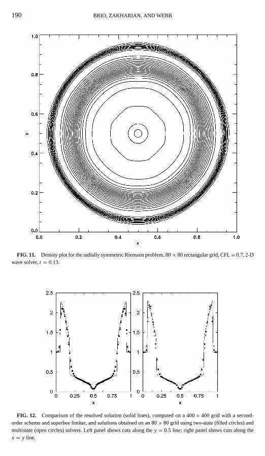
We have used a second-order scheme with the minmod-type limiter as outlined inSection 2. Figure 10 shows contour plots of the density att = 0.13 computed using a2-state linear solver on an 80× 80 rectangular grid. The Courant number in this example is0.7, which is the maximum for the 2-state solver. Figure 11 shows the solution to the sameproblem computed using multistate solver with CFL= 0.7 (maximum CFL in this case is1.0). Figure 12 shows 1-D cuts along they = 0.5 andx = y lines compared with the highlyresolved solution. It shows that the solution is more isotropic, and the radius of curvatureof the shock at angles not aligned with grid lines is more uniform.

The next example is a two-dimensional Riemann problem that produces double Machreflection and a shock propagating at the angle to the grid lines. Initial data in the four

186 BRIO, ZAKHARIAN, AND WEBB

FIG. 7. Density, rectangular grid, CFL= 0.6, 2-D wave solver,t = 0.52, enlarged.

quadrants are given by, e.g., [11],

ρ = 1.5, p = 1.5, u = 0.0, v = 0.0 if x > 0, y > 0

ρ = 0.5323, p = 0.3, u = 0.0, v = 1.206 ifx > 0, y < 0

ρ = 0.5323, p = 0.3, u = 1.206, v = 0.0 if x < 0, y > 0

ρ = 0.1379, p = 0.029, u = 1.206, v = 1.206 ifx < 0, y < 0.

Solutions for this case were computed on a 400× 400 rectangular grid to timet = 0.6using a second-order-accurate scheme and CFL= 0.5. Figures 13 and 14 demonstrate thedifference in the resolution and position of the mushroom cap that forms due to the interac-tion of the dense stream and postshock flow behind the oblique shock. The solution obtainedusing the multistate solver is closer to the high-resolution solutions in [11] computed withthe less diffusive monotonized central-difference and superbee limiters. Note that for thesecond-order scheme the change in the amount of the numerical diffusion due to differentlimiters may be comparable to the difference between the methods with and without 2-Dwave corrections.

The multistate solver adds two additional flux calculations per cell edge. In addition,for second-order accuracy in time, the multistage integration was used. The number ofexpensive function evaluations used in the multistate solver varies depending on the problem.Overall efficiency (CPU time required to achieve the same quality of the solution) ranged

MULTIDIMENSIONAL RIEMANN SOLVER 187

FIG. 8. Density, rectangular grid, CFL= 1.0, 1-D solver,t = 0.52, enlarged.

from 100% improvement in the first example to 50% decrease for the third example. Incomparison, CLAWPACK is based on Lax–Wendroff-type time differencing with transversewave propagation and requires three one-dimensional Riemann problems per interface, withonly a single time update. It is also more cost efficient. Solvers that do not require solutionof the Riemann problems, such as kinetic and flux-vector splitting schemes, are generallyseveral times less expensive. In addition, for such solvers, increased cost of only 20% dueto multidimensional corrections was reported by Fey [6].

5. CONCLUSIONS

In this paper we have obtained an exact solution of the multistate Riemann problem intwo dimensions for the linearized Euler equations of gas dynamics and have utilized it inthe construction of a numerical scheme. The numerical flux in our scheme generalizes theone-dimensional flux by introducing multidimensional wave contributions from the cornersof the computational cell. These waves are computed using a multistate linearized Riemannproblem and the formulas are suitable for finite volume applications on arbitrary grids.

The numerical experiments demonstrate that the additional information improves stabilityand reduces numerical diffusion of the scheme. The effect becomes more pronounced forlarge CFL numbers. The method also reduces anisotropy of the numerical diffusion and thegrid alignment of the numerical solution.

188 BRIO, ZAKHARIAN, AND WEBB

FIG. 9. Density, rectangular grid, second-order resolved solution,t = 0.52, enlarged.

APPENDIX

In this appendix we describe in more detail solution of a linear multistate Riemannproblem. In particular we calculate the integrals in the expression (11) for the pressure,p. Since the problem is linear, the solution can be written as a superposition of the dataconcentrated in a single sector of arbitrary angle. Therefore it is sufficient to work out theformulas for one of the sectors.

First we note that for the regionS1, shown in Fig. 3, the initial value problem reduces tothe one-dimensional wave equation for both pressure and velocity, and the solution can bewritten as

p(r , t) = p(r , 0)+ 1

2[sign[sin(φ − φi )]1pi + ρcs(ni ·1ui )],

u(r , t) = u(r , 0)+ 1

2ni

[1pi

ρcs+ sign[sin(φ − φi )](ni ·1ui )

], (1)

ρ(r , t) = ρ(r , 0)+ (p(r , t)− p(r , 0))/

c2s,

where indexi corresponds to the line of discontinuityl i = (cos(φi ), sin(φi )) in the ini-tial data,1pi = pi+1− pi , and1ui = ui+1− ui . Position vectorr = (x, y) = (r cos(φ),r sin(φ)) refers to the origin at the pointO, ni = (−sin(φi ), cos(φi )) is the unit normal to

MULTIDIMENSIONAL RIEMANN SOLVER 189

FIG. 10. Density plot for the radially symmetric Riemann problem, 80× 80 rectangular grid, CFL= 0.7, 1-Dsolver,t = 0.13.

the linel i . For regionS2 (see Fig. 3), the solution is a superposition of the correspondingone-dimensional waves.

For regionS3 the solution to the wave equation for pressure can be written as

p(x, y, t) = 1

2π cs

∂

∂t

∫ξ

∫η

p0(ξ, η)dξ dη√c2

st2− (x − ξ)2− (y− η)2 (2)

− ρcs

2π

∫ξ

∫η

∇ · u0 dξ dη√c2

st2− (x − ξ)2− (y− η)2 , (3)

where integration is over the area(x − ξ)2− (y− η)2 ≤ c2st2. Consider the first integral in

the expression above, converted to polar coordinates,

1

2π cs

∂

∂t

∫ξ

∫η

p0(ξ, η)√c2

st2− (x − ξ)2− (y− η)2 dξ dη

= p0(x, y)+ 1

2π cs

∂

∂t

∫ξ

∫η

p0(ξ, η)− p0(x, y)√c2

st2− (x − ξ)2− (y− η)2 dξ dη

= p0(x, y)+ 1

2π cs

∂

∂t

∫ 2π

0

∫ r+

0

1p0(φ′)r ′√−r ′2+ 2 cos(φ′ − φ)rr ′ + c2

st2− r 2dr ′ dφ′,

190 BRIO, ZAKHARIAN, AND WEBB

FIG. 11. Density plot for the radially symmetric Riemann problem, 80× 80 rectangular grid, CFL= 0.7, 2-Dwave solver,t = 0.13.

FIG. 12. Comparison of the resolved solution (solid lines), computed on a 400× 400 grid with a second-order scheme and superbee limiter, and solutions obtained on an 80× 80 grid using two-state (filled circles) andmultistate (open circles) solvers. Left panel shows cuts along they = 0.5 line; right panel shows cuts along thex = y line.

MULTIDIMENSIONAL RIEMANN SOLVER 191

FIG. 13. Density, double Mach reflection problem, 400× 400 rectangular grid, 1-D solver,t = 0.6.

wherer+ is the distance between the evaluation point(x, y) and the sonic wave front,

r+ = r cos(φ′ − φ)+√

c2st2− r 2 sin2(φ − φ′)).

Integration with respect tor ′ gives∫ r+

0

r ′√−r ′2+ 2 cos(φ′ − φ)rr ′ + c2st2− r 2

dr ′

=√

c2st2− r 2+ r cos(φ′ − φ)

(π

2+ arctan

r cos(φ′ − φ)√c2

st2− r 2

).

Dropping the term that is independent of the time and integrating with respect toφ′ weget

∫ φi+1

φi

(√c2

st2− r 2+ (r cos(φ′ − φ)) arctanr cos(φ′ − φ)√

c2st2− r 2

)dφ′

= r sin(φ − φ′) arctanr cos(φ′ − φ)√

c2st2− r 2

∣∣∣∣∣φi+1

φi

+ cst arctan

(√1− r 2

c2st2

tan(φ − φ′))∣∣∣∣∣

φi+1

φi

.

192 BRIO, ZAKHARIAN, AND WEBB

FIG. 14. Density, double Mach reflection problem, 400× 400 rectangular grid, 2-D wave solver,t = 0.6.

The second term is discontinuous atφ − φ′ = ±π2 and therefore if it is within the limits

of integration, it will contributeπ2 to the definite integral. Thus, the interval of integrationis split into regions where both the initial data and antiderivative are continuous. Finally,taking the time derivative and summing over all initial states the integral in Eq. (2) becomes

1

2π

m∑i=1

1pi Fi ,

whereFi is

Fi = π

2(1+ sign[cos(φi − φ)])sign[sin(φ − φi )] − arctan

(√1− r 2

c2st2

tan(φ − φi )

).

The integral (3) in the expression for the pressure is a line integral along each ofl i and canbe computed as

ρcs

2π

∫ξ

∫η

∇ · u0 dξ dη√c2

st2− (x − ξ)2− (y− η)2

= ρcs

2π(ni ·1ui )

∫ r+(φi )

0

1√−r ′2+ 2 cos(φi − φ)rr ′ + c2

st2− r 2dr ′

MULTIDIMENSIONAL RIEMANN SOLVER 193

FIG. 15. Density, solution to the linear 2-D Riemann problem,t = 0.15.

= ρcs

2π(ni ·1ui )

(π

2+ arctan

r cos(φi − φ)√c2

st2− r 2

)

= ρcs

2π(ni ·1ui )Gi ,

whereGi is

Gi = arctan

(l i · r√

c2st2− r 2

)+ π

2.

Combining formulas for (2) and (3) we obtain the pressure:

p(r , t) = p(r , 0)+ 1

2π

m∑i=1

1pi Fi + ρcs

2π

m∑i=1

(ni ·1ui )Gi .

To find velocity we take the gradient of the expression forp followed by integration intime. Applying this to the first integral (2) results in the expression (3), which was computedabove, with∇ · u0 replaced by∇ p0. That evaluates to the term proportional to1pi Gi .

194 BRIO, ZAKHARIAN, AND WEBB

FIG. 16. Comparison of the exact and numerical solutions to the linear 2-D Riemann problem,t = 0.05.

Noting that the gradient and time integration of (3) can be carried out using an explicitformula forGi , we obtain the expression

u(r , t) = u(r , 0)+ 1

2π

m∑i=1

(ni · wi

l i · wi

),

where

wi = (ni ·1ui )Fi + 1pi

ρcsGi

(ni ·1ui ) log(

r

cst +√

c2st2−r 2

) .

The logarithmic term is due to the vorticity mode present in the initial data. Finally, thedensity can be determined as in (1).

The example in Fig. 15 shows the exact solution to the linear Riemann problem fordensity att = 0.15, with the initial data consisting of three states,

ρ = 2.0, p = 6.0, u = 1.2, v = 0.18 if y > 0 andy >√

3x

ρ = 1.0, p = 2.2, u = −2.3, v = 1.0 if x > 0 and|y| < √3x

ρ = 4.0, p = 8.5, u = 0.3, v = 0.38 if y < 0 andy < −√3x.

Figure 16 is the exact solution of the pressure and velocity att = 0.05 along the linex =0.03 for the same problem together with the numerical solution obtained usingMacCormack’s scheme applied to the linearized Euler equations of gas dynamics.

MULTIDIMENSIONAL RIEMANN SOLVER 195

ACKNOWLEDGMENT

The work of G.M.W. was supported in part by NASA Grant NAG5-5180.

REFERENCES

1. R. Abgrall, Approximation du probl`eme de Riemann vraiment multidimensionnel des `equations d’Euler parune methode de type Roe, I: La lin`earisation,C.R. Acad. Sci. Ser. I319, 499 (1994); 499–504; II: Solution duprobleme de Riemann approch`e,C.R. Acad. Sci. Ser. I319, 625.

2. M. Brio and J. K. Hunter, Mach reflection for the two-dimensional Burgers equation,Physica D60, 194(1992).

3. T. Chang and L. Hsiao,The Riemann Problem and Interaction of Waves in Gas Dynamics(Wiley, New York,1989).

4. P. Collela, Multidimensional upwind methods for hyperbolic conservation laws,J. Comput. Phys.87, 171(1990).

5. S. F. Davis, A rotationally biased upwind difference schenme for Euler equations,J. Comput. Phys.56, 65(1984).

6. M. Fey, Multidimensional upwinding. 1. The method of transport for solving the Euler equations,J. Comput.Phys.143, 159 (1998).

7. M. Fey, Multidimensional upwinding. 2. Decomposition of the Euler equations into advection equation,J. Comput. Phys.143, 181 (1998).

8. H. Gilquin, J. Laurens, and C. Rosier, Multi-dimensional Riemann problems for linear hyperbolic systems,Notes Numer. Fluid Mech.43, 284 (1993).

9. E. Godlewski and P.-A. Raviart,Numerical Approximation of Hyperbolic Systems of Conservation Laws(Springer-Verlag, New York, 1996).

10. S. Canic, B. L. Keyfitz, and D. H. Wagner, A bifurcation diagram for oblique shock interactions in the unsteadytransonic small disturbance equation, inProceedings of the Fifth International Conference on HyperbolicProblems: Theory, Numerics, Applications, edited by J. Glimmet al. (World Scientific, Singapore, 1994).

11. R. J. LeVeque, Wave propagation algorithms for multidimensional hyperbolic systems,J. Comput. Phys.131,327 (1997).

12. D. W. Levy, K. G. Powell, and B. van Leer, Use of rotated Riemann solver for two-dimensional Euler equations,J. Comput. Phys.106, 201 (1993).

13. W. B. Lindquist, The scalar Riemann problem in two spatial dimensions: piecewise smoothness of solutionsand its breakdown,SIAM J. Math. Anal.17, 1178 (1986).

14. D. De Zeeuw and K. Powell, An adaptively refined cartesian mesh solver for the Euler equations,J. Comput.Phys.104, 56 (1993).

15. P. L. Roe, Approximate Riemann solvers, parameter vectors and difference schemes,J. Comput. Phys.43,357 (1981).

16. P. L. Roe, Discrete models for the numerical analysis of time-dependent multidimensional gas dynamics,J. Comput. Phys.63, 458 (1986).

17. P. L. Roe,Linear Advection Schemes on Triangular Meshes, Tech. Rep. CoA, Rep. No. 8720 (Cranfield,1987).

18. C. B. Rumsey, B. van Leer, and P. L. Roe, A multidimensional flux function with applications to the Eulerand Navier–Stokes equations,J. Comput. Phys.105, 306 (1993).

19. B. van Leer, Towards the ultimate conservative difference scheme: V. A second order sequel to Godunov’smethod,J. Comput. Phys.32, 101 (1979).

20. D. H. Wagner, The Riemann problem in two space dimensions for a single conservation law,SIAM J. Math.Anal.14, 534 (1983).