Two-Dimensional king Correlations: The SMJ Analysis*tracy/selectedPapers/1… · ·...
57
ADVANCES IN APPLIED MATHEMATICS 4,46- 102 (1983) Two-Dimensional king Correlations: The SMJ Analysis* JOHNPALMER Department of Mathematics, University of Arizona, Tucson, Arizona 85721 AND CRAIG TRACY Department of Muthematics, Dartmouth College, Hanover, New Hampshire 03755 INTRODUCTION In this paper we make rigorous the analysis by Sato, Miwa, and Jimbo (henceforth, SMJ) [25-281 of the two-dimensional, zero external field Ising correlations. We also make use of this analysis to complete the verification of the Osterwalder-Schrader axioms (see [8]) for the correlations scaled from below T, by establishing rotational invariance in this case (Theorem 6.6). In [3, 31, 321Wu, McCoy, Tracy, and Barouch (WMTB) discovered that the scaled two point functions for the two-dimensional Ising model are expressible in terms of a Painled function of the third kind. This discovery was made by using results from the thesis of Myers [21] (which was in part based upon earlier work by Latta [16]) who established a connection between a linear integral equation arising in the problem of electromagnetic scattering from a strip and a differential equation of Painleve type. A summary of the Latta-Myers method can be found in Appendix B of WMTB. Later in [ 191McCoy, Tracy, and Wu improved the mathematical foundations of the two point function analysis, and developed connection formulas for a family of solutions to the Painleve equation. In an impressive seriesof papers, SMJ generalized the two point function result to the higher correlations, and these authors found what we believe is certainly the natural setting for these results. For an overview of this work, the reader will find [12] helpful. They were aware that all the Painleve transcendents arise naturally in the integration of the simplest of the Schlesinger equations for monodromy preserving deformations of linear *Supported in part by the National Science Foundation under Grant MCS-8102536. 46 0196-8858,‘83 $7.50 Copyright @ 1983 by Academic Press, Inc. All rights of reproduction in any form reserved.
Transcript of Two-Dimensional king Correlations: The SMJ Analysis*tracy/selectedPapers/1… · ·...
ADVANCES IN APPLIED MATHEMATICS 4,46- 102 (1983)
Two-Dimensional king Correlations: The SMJ Analysis*
JOHNPALMER
Department of Mathematics, University of Arizona, Tucson, Arizona 85721
AND
CRAIG TRACY
Department of Muthematics, Dartmouth College, Hanover, New Hampshire 03755
INTRODUCTION
In this paper we make rigorous the analysis by Sato, Miwa, and Jimbo (henceforth, SMJ) [25-281 of the two-dimensional, zero external field Ising correlations. We also make use of this analysis to complete the verification of the Osterwalder-Schrader axioms (see [8]) for the correlations scaled from below T, by establishing rotational invariance in this case (Theorem 6.6).
In [3, 31, 321 Wu, McCoy, Tracy, and Barouch (WMTB) discovered that the scaled two point functions for the two-dimensional Ising model are expressible in terms of a Painled function of the third kind. This discovery was made by using results from the thesis of Myers [21] (which was in part based upon earlier work by Latta [16]) who established a connection between a linear integral equation arising in the problem of electromagnetic scattering from a strip and a differential equation of Painleve type. A summary of the Latta-Myers method can be found in Appendix B of WMTB. Later in [ 191 McCoy, Tracy, and Wu improved the mathematical foundations of the two point function analysis, and developed connection formulas for a family of solutions to the Painleve equation.
In an impressive series of papers, SMJ generalized the two point function result to the higher correlations, and these authors found what we believe is certainly the natural setting for these results. For an overview of this work, the reader will find [12] helpful. They were aware that all the Painleve transcendents arise naturally in the integration of the simplest of the Schlesinger equations for monodromy preserving deformations of linear
*Supported in part by the National Science Foundation under Grant MCS-8102536.
46 0196-8858,‘83 $7.50 Copyright @ 1983 by Academic Press, Inc. All rights of reproduction in any form reserved.

PALMER AND TRACY 47
differential equations (for a useful account of this connection see Flaschka and Newell [7]). There is no obvious candidate for an ordinary differential equation to associate with the Ising model. However, it is a relatively straightforward calculation that the Clifford algebra which plays a decisive role in the Onsager-Kaufman [14, 15, 221 analysis of the Ising model scales to the Clifford algebra associated with the free Dirac field in two space-time dimensions. This free field satisfies the Dirac equation; and by making inspired use of this observation, SMJ succeed in showing that the differen- tial equation encountered in the two point function analysis arises as a particular case of a monodromy preserving deformation for a space of (multivalued) solutions to the Euclidean Dirac equation. More specifically, they introduce a family of single valued solutions to the Dirac equation in Minkowski space whose analytic continuation to the Euclidean domain is multivalued with branch points at a,, . . . a, E R*. The solutions they write down have monodromy which is formally determined by the commutation relations between the spin fields and the Dirac field. When the branch points a,, . . . , a, are moved, this monodromy remains unchanged. They develop a local operator product expansion which enables them to calculate the Fourier series expansion of the Minkowski wave functions about the points which “map” into a,, . . . , a, under analytic continuation. Under the analytic continuation to the Euclidean region, these Fourier coefficients suggest that the Euclidean solutions have restricted singularities at the branch points a,, . . . , a, and that the lowest order coefficients are com- putable in terms of scaled correlations and their derivatives (involving both “order” and “disorder” variables).
In [26] SMJ provide a penetrating analysis of monodromy preserving deformations of families of solutions to the Euclidean Dirac equation. One of the principal conclusions of their work is that the low order Fourier coefficients satisfy a total system of differential equations (the deformation equations). In the case of just two points a, and u2, they reproduce the WMTB result in this manner.
In this paper our principal results concern the construction of the Euclidean wave functions. In [27] there do not seem to be any convergence results that would help make analytical sense of the construction for the Minkowski wave functions which is proposed. We believe the same can be said for the local operator product expansions in the Minkowski regime, and for the control of the analytic continuation to the Euclidean region. Here we circumvent these difficulties by first defining lattice analogues of the Euclidean wave functions. We then use results from [23] and [24] to control the convergence to continuum wave functions in the scaling limit. Because these functions are multivalued, the direct definition in the Euclidean region naturally leads to more than one analytical expression. In our approach, it is only the control of the convergence of the lattice wave

48 ISING CORRELATIONS
functions which guarantees that these many expressions for the continuum wave functions piece together consistently (Theorem 4.2). We avoid the local operator product formalism by scaling lattice formulas for normal ordered products and using results from [23] to establish an effective expression of continuity in the resulting limits (Theorem 4.1). The local Fourier expansion coefficients may then be computed directly, although at the cost of additional complications compared with the analogous SMJ calculation in the Minkowski regime (Theorem 5.1).
The first five sections of this paper are devoted to a proof of Theorem 5.1. Many of the details in the proofs are fussy rather than delicate but there are a few matters of independent interest we would like to mention. The first is that the lattice wave functions we define do satisfy a linear difference equation everywhere except on the branch cuts to the right of the points a,,..., a,. This is a simple calculation everywhere except on the horizontal rays to the left of the points a,, . . . , a,. At such points this result depends on the “local” character of the induced rotation for the transfer matrix. This property is ultimately responsible for the fact that the scaled wave functions satisfy the Euclidean Dirac equation on the horizontal rays to the left of the points a,,. . . , a, even though the lattice wave functions seem abruptly glued together along these rays in our definition.
The proper identification of the low order Fourier coefficients requires some identities for the derivatives of the scaled correlations (see Theorem 4.3). In SMJ such identities are deduced using the result that a particular integral operator kernel reduces to a product kernel in right coordinates in the continuum limit. Here we deduce these identities by scaling difference identities on the lattice. These difference identities (see Theorem 2.0) are of some interest since they are the sort of identities needed to make the connection between the Clifford algebra formalism developed here and the Montroll, Potts, Ward [20] formulas for the correlations in the Pfaffian formulation.
In the final section of this paper, we provide a review of some of the results in SMJ [26, 271. We make no claim to originality here since virtually every argument can be found somewhere in either SMJ [26] or SMJ [27]. We should perhaps mention here that we find the level of mathematical rigor in SMJ [26] and SMJ [27] rather different. We do not imagine that we have in any way improved on the mathematics in SMJ [26]. On the other hand, our confusion about the status of the work in SMJ [27] directly inspired the present effort. What we have done in the final section is present a simplified account of SMJ [26] leading as directly as possible to the deformation equations and the differential equation (6.26) for the logarithm of the correlation function. Recently Kadanoff and Kohmoto [13] have given a similar presentation of these results. However, partly because we did not understand their calculation of the diagonal elements Akk in the two point

ISING CORRELATIONS 49
function analysis, and partly because we wished to emphasize more mathematical aspects of the subject we feel justified in presenting our account. In particular, the connection between the deformation equations for F and G and the complete integrability of the extended holonomic system dW = 02w is not mentioned in the Kadanoff-Kohmoto paper. We believe this connection provides an important clue for determining “boundary conditions” that might single out the particular solution of the deformation equations which is of interest. The problem of “boundary conditions” for the deformation equations is unsettled except for the two point case (see MTW [19]). The reader interested in this problem should be aware of the construction in SMJ [26] of solutions to the extended system dW = Q2w with generalized monodromy but the same deformation equa- tions. For reasons of space and simplicity, this is not described in Section 6 of this paper. We recommend that the reader start with Section 6 of this paper or Kadanoff and Kohmoto [ 131 for orientation before proceeding with the developments in Sections 1-5.
In conclusion, we would like to mention some lines of research since the pioneering work of Myers, where Painleve transcendents have been intro- duced to solve applied problems: (i) Bariev [2] has evaluated the scaled spontaneous magnetization of the half plane Ising model in terms of Painleve transcendents of the third kind; (ii) Jimbo, Miwa, Mori, and Sato [ 1 l] express the density matrix of the one dimensional impenetrable boson model of Lenard [17] and Schultz [29] in terms of a certain Painleve transcendent of the fifth kind; (iii) these authors also note that the solutions of the same Painleve equation with different boundary conditions can be used to compute properties of random matrices which are of interest in the statistical theory of energy levels; (iv) Creamer, Thacker, and Wilkinson [6] employing the quantum inverse method express the density matrix of the delta function gas of Lieb and Liniger [ 181 as a perturbation expansion in powers of l/c (c is the coupling constant), and the explicit evaluation of the (l/c) term involves the fifth Painleve transcendent mentioned in (ii) as does the (l/c)* term in the later work of Jimbo and Miwa [lo] and of Creamer [5]; (v) starting with Ablowitz and Segur [l], several authors have made use of the second Painlevi: transcendent in the asymptotic analysis of the Korteweg-deVries (and related) equations; and finally, (vi) in the area where it all began, Jimbo, Kashiwara, and Miwa [9] employed these functions to study the electromagnetic scattering from a disk.
1
We begin with a description of the Fock representations in terms of which we will characterize the Ising correlations. Let W denote a complex Hilbert

50 PALMER AND TRACY
space with complex structure i and distinguished conjugation P. Suppose Q is a self-adjoint idempotent on W such that QP + PQ = 0. Let P,= (l/2)( I f. P), Q * = (l/2)( I f Q) and W, = Q * W. The Q-Fock represen- tation of the Clifford relation on (W, P) is W 3 w + F(w) = a*(Q+w) + u(Q _ w), where ~7 = Pu and a*( .) and a( ‘) are the standard creation and annihilation operators on A( W,), the complex alternating tensor algebra over W, [4]. One may easily check that F( u)P( w) + I;( w)F( U) = (u, Pw)l; these are the generator relations for the Clifford algebra C(W, P).
The complex structure i maps P- W onto P, W. If we let X = P, W, then themapI$(-iI): P+W@P-W + X $ X establishes a real orthogonal equivalence between W and X @ X. The complex structure i becomes
0 [ I
-’ on%@ XandPbecomes A 1 0 [ I -y . Since iQ commutes with both
P and i it follows that iQ has the matrix representation [ 1 t i onX@X. Since iQ is a complex structure it follows that A must be a complex structure on x. The matrix representation of Q is thus - i(iQ) = [ _ i t].
Now consider the real orthogonal map D = 2 -r12[: -:I. Then D is a
unitary map from (XeX,i) to (~CCYC,~~(-~)), DPD*=[y i]
and DQD* = 0’ [ 1 -“I . We will refer to (X $ X, A $ (-A)) as the Q representation of W since Q is diagonal in this representation.
DEFINITION. G( W, Q) will denote the set of bounded operators on A( W,) such that gP( w) = P(‘(T(g)w)g for some bounded invertible P- orthogonal T(g) on W (a P-orthogonal is a map which preserves the complex bilinear form ( * , P * )).
Because the {F(w) ] w E W} generates an irreducible algebra on A( W,) [30], the map g is determined up to multiplication by a constant by T(g). We shall refer to T(g) as the rotation induced by g. The semigroup G( W, Q) is of interest to us because both the transfer matrix and the spin operator for the two-dimensional Ising model may be realized as elements of G( W, Q) for suitable (W, Q). We turn next to the characterization of the Ising correlations given in [24].
Let Z denote the set of all integers,and write Z ,,2 = Z + (l/2). We let X be the real Hilbert space Z2(Z,,,, W2) and W the complexification of X which may naturally be identified with Z2(Z,,,, C’). The distinguished conjugation on W is ordinary complex conjugation. The interaction con- stant K = J/kT, where T > 0 denotes the temperature, k the Boltzmann constant, and J a coupling constant. In this paper, J will be considered fixed, and we will parametrize “temperature” dependent quantities by T to conform with usage in physics. The critical point for the Ising model occurs at K, = (1/2)ln(l + a) and the corresponding temperature will be de- noted by T,. Define the dual interaction constant K* by sh 2K*sh 2K = 1,
ISING CORRELATIONS 51
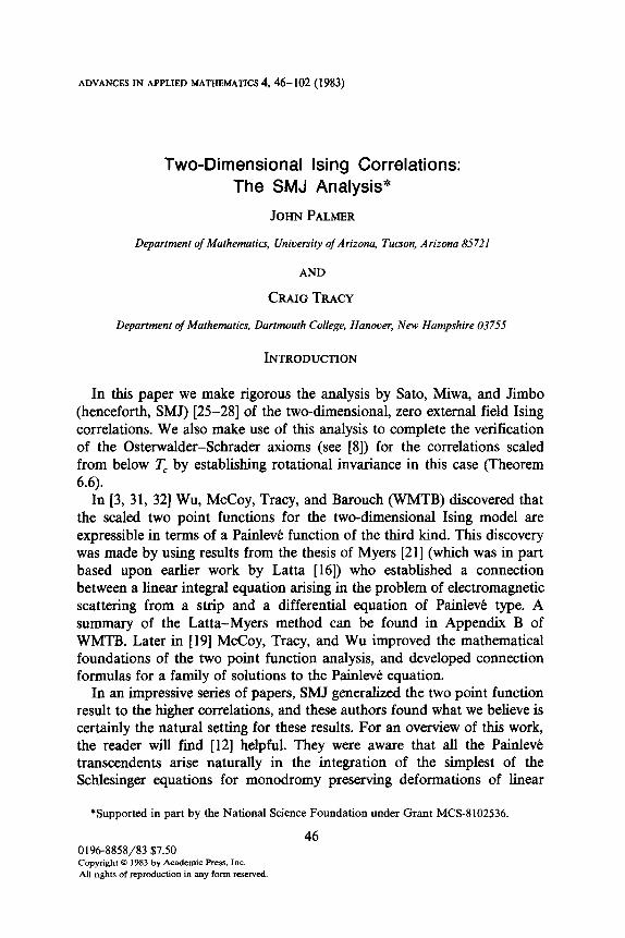
and let s1 = sh2K*, c, = ch2K*, s2 = sh2K, and c2 = ch2K. We write P = kK*/J. When T > T, it follows that P < T, and vice versa.
ForfE Wlet
j-(e) = (1/2n) c f(k)eike. kaZ,/,
The rotation, T, induced by the transfer matrix is defined by
?y(8) = [
ClC2 - cam e s,sine - i(c, - c,cod)
s,sin 8 + i( c2 - c,c0s e) cam e I 9
ClC2 -
fie) = T(e)f(e) (1.1)
For future reference we include here the action of T on the complex orthonormal basis
Te,(k) = - (1/2)e,(k - 1) + c1c2e,(k) - (1/2)e,(k + 1)
-(i/2)(c, - s,)e,(k - 1) + ic,e,(k)
-(iP)(c, + Sl)e2(k + l),
Te,(k) = -(1/2)e,(k - 1) + c,c2e2(k) - (1/2)e,(k + 1)
+(i/2)(c, + s,)e,(k - 1) - ic,e,(k)
+(i/2)(c, - s,)e,(k + 1).
0.2)
Following Onsager [22] we introduce functions y( 0) > 0 and a( 0) (called 6*(w) by Onsager) defined by
thy(e) = clc2 - COST,
shy(8)ei@) = (c2 - C,COS e) + is,sinf3 (1.3)
Substituting (1.3) in (1.1) one finds
T(e) = exp y(e) ie-!acBj +~a(e) [ 1 11 .
The map Q on W is multiplication by
Q(e) = [ -ie!iate, iei;e)]
in the Fourier transform variables. If we let T,= Q + T, then V = I $ T,

52 PALMER AND TRACY
@(T+@ T,) 63 * * * on A( IV,) is an element of G( IV, Q) such that T(V) = T. The map V will be referred to as the transfer matrix.
We define a family of real orthogonal maps sm on W by
s,ej(k) = sgn(m - k)ej(k), m E E, k E E,,,.
In [24] it was shown that for T < c there exists an element a,,, E G( IV, Q) such that T(u,,,) = s,. The map am is uniquely determined by this condition and the further no~~~tions ui = I and (a,& 1) > 0. Here 1 denotes the vacuum vector 1 @ 0 $ 0 . . e E A(W+). We refer to a, as a spin operator on A( IV+).
Suppose now that a E H2, we define a(a) = V”*UJ-~~. Since Vb is an unbounded operator when b < 0, it requires some care to define o(a) as an operator. In this paper we will be interested in “time ordered” products of the operators a(a). In such products the power of the transfer matrix V sandwiched between two spin operators is always nonnegative, and the transfer matrices on the ends of such products encounter the vacuum state with the result I’*1 = 1. For our purposes then the symbol a(a) may be understood as a convenient notational device. In Section 2 we will show that, in any case, a(a) does extend naturally to an element of G(W, Q).
At this point it is convenient to introduce the time ordering symbol ‘5, Suppose ~,(a,) (1 = 1,. . . , r) is a collection of operators on A (IV,) depend- ing on the parameters a, E BP*, and write ?(a[) for the j’th component of a,. If all the second components are distinct (that is n2(u,) * 7c2( a,) unless E=m)thenwewrite
“j;pl(%> * * * %W = ‘Ps(,)(%(i)) * * * %&,fr,h
where the permutation, s, of (1,. . . , r) is chosen so that rr~(us~,~) < rr2(usC29 * + * < ~2(%(r)).
In [24] it was proved that the “plus” state infinite volume correlations below the critical temperature are given by
ht, . . * q&T, = @J(q) *** u(a,)L l)T, 0.4)
with 1 the vacuum in A(W+). To simplify notation we will commonly omit the vacuum vector 1, writing (Al, 1) = (A).
The reader should note that the right-hand side of (1.4) depends on the temperature, since both the transfer matrix and Q depend on T through (1.1) and (1.3). Since the spin operators a, and u, commute, it follows that the time ordered product in (1.4) is unambiguous even when there are coincidences among the second coordinates nz( a,) (I = 1,. . . , r). In such circumstances (1.4) still represents the spin correlations.
Now let pk = ~~(e,(k)) and qk = $%F(ez(k)), and define iu - (W QP, + 4sh .KhJ~~+,,2 tk f Zl,d. If a E Zlj2 x 2 then f as ab&i 7

ISING CORRELATIONS 53
we introduce the notation P(Q) = Pp,,l/ -‘*. The infinite volume corre- lations for the Ising model above the critical temperature are given by [24]
+a, * - . %,)T>T, = (%b,) . * * PWL IL*. (1.5)
The vacuum expectation on the right is evaluated at temperature T* -c T,. As above, because p,,,~,, = p,,prn (this needs to be checked!) the time ordered product is unambiguous even when there are coincidences among the coordinates 7r1(u,). The spin correlations continue to be represented by (1 S) in such circumstances.
We now introduce the lattice analogues of free Fermi fields at imaginary times. The reason for introducing linear combinations of pk and qk rather than working directly with ( pk, qk) has to do with a simplification in the analysis of the monodromy for the associated Euclidean Dirac equation that will appear later. Suppose x E h ,,2 x H, we define
4+> = F(Wj(x,)), j = f 1, (1.6)
wherefj(k) = 2-‘I*[-je,(k) + e,(k)]. Let v,f(x) = (1/2Kf(x, + 1, xd -t-(x, - 1, x2) and VAX) =
(1/2)(f(x,, x2 + 1) -f(x,, x2 - 1)). Then ‘,(X) [ 1 G-I(X) satisfies the following
lattice version of the Euclidean Dirac equation:
where
This is most easily checked by computing
representation of W making use of iF
0 -i]v2[ J:rl,] in the Q r) = F(R @ (-R)e) and
sh y( O)eia(@ = ( c2 - c,cos 8) + is,sin 0. As may be easily verified, the com- plex structure A is multiplication by form variables for X = 12(h,,,,
[ $,, -“@,
3 in the Fourier trans-
BP*), and the rztation T, induced by the transfer matrix, becomes multiplication by
[ ‘-‘(‘, ’
I on%@ XintheQ
representation of IV. One should also note ihat $&) 2-‘/‘[fi(x) @fj(x)] in the Q representation.
goes to Ofi =
We are now prepared to define the lattice order-disorder correlations whose scaled versions play a decisive role in the SMJ analysis of the Ising correlations.

54 PALMER AND TRACY
Let s denote an integer from 1 to r. Suppose that x, a, E Z,,, x Z and a,EZ2forI= l,..., r, I * s. Suppose that the second coordinates ~~(a[) (I= l,..., r) are all distinct, and for convenience suppose ~~(a,) < T*(Q) . . . < ~~(a,). We define
There is no need to specify the order in the product l-‘llLsu(u,), since this is controlled by the time ordering symbol. We will be interested in w,!(x, a) as a function of (x, j) with s = 1,. . . , r and a = (a,, . . . , a,) held fixed. In particular, it is interesting to see what happens when am agrees with ?r2(u,) for some a, (I = l,..., r). Since #j(k,O)u, = sgn(l- k)u,rl;.(k,O) and lC;.(k,O)pL, = -sgn(s - k)~&~(k,O) (k * s) it follows that the natural extension of w,?(x, a) to points where am agrees with rz( a,), for some a,, is a two-valued function. The definition of w,!(x, a) was split into two parts so that the “branch cuts” for w;(x, a) lie on the horizontal rays to the right of each of the points a,. If x makes a local circuit of a, starting on the horizontal ray to the right of a, and moving counterclockwise, then when it returns to its starting point w,T(x, a) has changed by a sign. Since we do not have a notion of continuity on the lattice this monodromy property may not seem significant. However, the reader should note that as a consequence of (1.6) the function y?(x, a) satisfies an elliptic difference equation as a function of (x, j), at least away from the points where V*(X) agrees with some rrr(ur). Actually, one may show that w,T(x, a) satisfies the same difference equation even when v~(x) = ~~(a,) as long as n,(x) < a,(~[). In the notation of Lemma 2.2 of [24] this follows from the fact that the only nonzero matrix elements of the commutator [s(l), T] connect the vectors {ej(l f 1/2)[j = 1,2}. This implies that y!(x, a) jumps in a highly “regular” fashion from one site to the next as x makes the local circuit of a, described above. One should also observe that as the points a,, . . . , a, are varied the monodromy of the solutions wjs(x, a) to the difference equation (1.6) remains fixed. In the continuum limit it is this monodromy preserving property that SMJ exploit [26, 271 to demonstrate that the scaled n-point functions satisfy nonlinear Pfaffian systems of differential equations. One might pursue a similar analysis on the lattice, but this will not be attempted here (a slightly different choice for wf(x, a) seems appropriate for such an analysis). Instead we will scale the functions wj(x, a) to their continuum limits using results from [23] and [24] to control the convergence. To avoid introducing extra notation we will use w,!( x, a) to denote the scaled counter- part of the lattice wave functions w;(x, a) when there is no cause for

ISING CORRELATIONS 55
confusion. Our principal results concern the following properties of the scaled functions WY”< x, a):
(1) The functions w;(x, a) satisfy the Euclidean Dirac equation in the variables (x, i) except at the points a,, where they have branch cuts and fixed monodromy as a, and s vary.
(2) The order of growth of $(x, a) is restricted at each singularity a, and the functions w,!(x, a) are exponentially small for x near 00.
(3) Let (r,, 6,) denote polar coordinates in W2 centered at a,. The “Fourier coefficients” of wy( r,, e,, a) in the 0, variables are Bessel functions of r, multiplied by functions of a = (a,, . . . , a,). The functions of a.~ R2’ which multiply the most singular (at r, = 0) Bessel functions are expressible in terms of scaled correlations for ~(a,), ~(a,) (m = 1,. . . , r) and their a, derivatives.
The precise statement of results will be given later. Conditions (1) and (2) will single out an r-dimensional family of solutions to the Euclidean Dirac equation [26] and (3) will permit us to show that {wi(x, a)]s = 1,. . . , r} is a basis for this finite-dimensional vector space. The general analysis of monodromy preserving deformations of the Euclidean Dirac equation in [26] coupled with the identification of n-point functions in (3) above determines Pfaffian systems of differential equations for the scaled n-point correlations.
Since the analysis we have just sketched is identical to that presented by SMJ [26,27], it might be useful for the reader to understand what contribu- tions we believe we have made to this analysis. In large measure what is novel in this paper concerns the definition of the functions wy(x, a) and the rigorous calculation of the local expansions in terms of scaled correlations. In [27] the wavefunction wy(x, a) is introduced as a multivalued analytic continuation of a single valued entity defined in the Minkowski region for x and a. A local operator product expansion is developed to compute the Fourier expansion coefficients in the Minkowski regime, and the results are analytically continued to the Euclidean region. While the intuition behind the two-valued nature of the analytic continuation is instructive, and the calculation of the expansion coefficients is simpler than the calculation presented here, we believe that a complete definition of the single valued Minkowski entity (valid almost everywhere in space-time) together with a rigorous account of the operator product expansion, the analytic continua- tion of the wave functions, and the validity of analytically continuing the Fourier coefficients would be a considerable undertaking.
By working directly with the “Euclidean” wave functions w;(x, a) we avoid problems associated with analytic continuation and we are able to exploit formulas from [23] and [24] which are valid almost everywhere.

56 PALMER AND TRACY
2
In this section we develop identities for the Ising correlation functions that we shall use later to obtain formulas for the derivatives of the scaled correlations. These identities will play an important role in properly identi- fying the low-order expansion coefficients of the wavefunctions y!( x, a). To state our main result we introduce some notation. Let P(k) = (ch K)p, + i(sh K)qk and Q(k) = (ch K)q, - i(sh K)p,. The difference identities we require are all consequences of the following result.
THEOREM 2.0. The map VuJ - ’ extend from an operator densely defined on the span of the product vectors lIj, k F( ej( k))l to a bounded operator on A( W+). The operator V - ‘uJ = (Vu,,V - ‘)* is a bounded operator on A( W,). Furthermore
(1) u1 = W/2)P(V%9
(2) 11.1/z = -iQ(1/Wm (3) Va,V - ’ = exp[ - 2K*iQ( 1/2)P( - l/2)10,, (4) v-I/t _ ,,*v = P*( - l/2)(7,.
Prooj The first identity may be easily verified by consulting the finite dimensional representation for pk and qk in the discussion following (1.4) in [24]. The argument needed to extend this identity to the infinite-dimensional situation is easily supplied (see below).
To prove (2) observe first that P,,~ = P(1/2)u,. It is a simple calculation to check that q(1/2)p(1/2) = Q(1/2)P(1/2). Thus P,,~ = P(1/2)(iQ(1/2) P(1/2)u,) = -iQ(1/2)u,.
Let T = T(V) be the rotation induced by the transfer matrix. Then V-‘lIj ,F(ej(k))l = Il,,,F(T-‘e/k))1 (the order of the terms in the product is irrelevant except that this order should be the same on both sides of the equality). We shall find a useful expression for Vu,,V - ’ by computing the induced rotation of u,VuOV -‘. This induced rotation is sTsT - ’ and it has a simple form because the commutator [s, T] has only a small number of non zero matrix elements in the basis {ej(k)}. We take advantage of this by writing sTsT -’ = I + K, from which we deduce that K = [s, T]sT -‘.
From (1.2) one easily computes
[s, T]e,(k) = -e,( - l/2) - i(c, - s,)e2( - l/2), k = l/2,
= e,(W) + i(c, + s,)e,(l/% k = -l/2, = 0, k z l/2, - l/2,
[s, T]e,(k) = -e2(- l/2) + i(c, + s,)e,( - l/2), k = l/2,
= -M/2) - i(c, - s&-,(1/2), k = - l/2, = 0, k * l/2, - l/2.
ISING CORRELATIONS 57
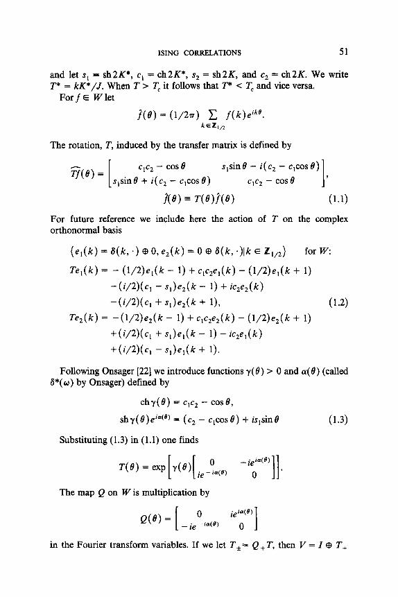
Since T is a P-orthogonal map we may determine its inverse by comput- ing its transpose. One finds that K is zero except on the subspace of vectors spanned by { ei( f l/2) lj = 1,2}. The induced rotation I + K is thus the identity on the complement of this subspace. The element of the Clifford group with induced rotation I + K may thus be expressed in terms of p( + l/2), and q( it l/2), and we proceed next with the calculation of this element along the lines of Theorem 1.1 of [23]. If U denotes the restriction of sTsT-’ to the span of {ej(& 1/2))j = 1,2) then the matrix of U in the (ordered) basis (e,(1/2), e,(1/2), e,(- l/2), e2(- l/2)) is
CI(C, - 4 -is, Cl icdc, - 3) -is, cdc, + s,> ic,(c, + 4 -Cl
-Cl -ic,(c, + s,) dc, + Sl) is, .
-ic,(c, - s,) Cl is, dc, - s,) _
Let
c,(c, - Sl> 0 Cl 0
0 c,(c, + s,> 0 G= -cl
-cl 0 dc, + 3) 0 ’
0 Cl 0 CI(C, - s,> _
0 -s, 0 c,(c* - s,) 0 0
H= -s, dc, + 4 0 -c,(c, + $1 0 SI
_ -+I - 5) 0 SI 0
Then the matrix U relative to the real orthogonal decomposition, span {ej( f l/2)} $ span{iej(* l/2)}, is G -z . Let A, denote the complex structure on the span of {ej( &- H/2)} I dl etermined b A,e,( f l/2) = e2( f l/2) and R,e,(f l/2) = -e,( f l/2). Let Q, = I0 -to be the
[ I
i I associated idempotent. We write D, = 2 -‘I2 : !i and make the trans-
0 formation to the Q, representation
The R matrix associated with U and A, is then
R= u:,-’ - 1 4 2u2; ’
u2;‘u2, 1 - u,;’

58 PALMER AND TRACY
Let I= [A ~1, J = [i -iI and define R, = [y L] and R, = [y -iI.
One may verify without difficulty that
i
- (UC,)4 R= -[(
Kc1 - Wc,lR* Cl + Wc,lR, I h/CI)RI *
According to Theorem 1.1 of [23], an element of the Clifford algebra with induced rotation U is given by 8 exp( l/2& Rf, A fk, where the sum is over any i-complex orthonormal basis of W, f = Pf, and 8 is the Q, normal ordering map from the Grassmann algebra over W onto the Clifford algebra, C(W, P) (see [23]). In the Q, representation i = A, @ (-A,). Thus if uj (j = l,..., 8) is the standard basis for WE, we may choose f, = u,,f2 = u3,f3 =& = u5, andf, =& = u,. One finds
exp(1/2)cRf, A fk = 1 - (1 - cc’ >f, *f* - (w&2 *A + fi A Jz> k
+ (1 + ci-‘)f, A&.
Making use of the fact that F(f,) = (l/2)( p(1/2) - iq(1/2)) and F(:(fi) = (l/2)( p( - l/2) - iq( - l/2)) it follows that
eexP(l/2)CRfk A fk = 1 + (2C,)-‘(P(1/2)P(-1/2) - q(i/2)q(-1/2)) k
+ (j/N1 + ~I/clMV2M- l/2). (2.1)
Now multiply the right hand side of (2.1) by c, and express the resulting element of the Clifford algebra in terms of P(k) and Q(k). One obtains
c, + is,Q(l/2)P( - l/2) = ch2K* + sh2K*iQ(1/2)P( - l/2)
= exp[2K*iQ(l/2)P(-l/2)].
We have then
= (const.)a0exp[2K*iQ(l/2)P( - l/2)]. (2.2)
By comparing the squares of both sides of this last equation we find (const.) = f 1. In Section 3 we will compute a normal ordered form for the right-hand side which will establish that (const.) = + 1.

ISING CORRELATIONS 59
Since I/ is a bounded self adjoint operator, F’ -I is a densely defined self-adjoint operator, and VuJ -’ extends to a bounded operator, it follows that V - ruJ = (VuJ - I)* is a bounded operator (i.e., the range of eO,Y is contained in the domain of I’ - ‘). If we take the adjoint of both sides of (2.2) we find
Vl/-‘u,V = exp[2K*iQ*(1/2)P*(- 1/2)]0,. (2.3)
Next we compute V-‘P(- 1/2)Vusing V-*F(x)V= F(T-lx):
PP(-1/2)V= c,P*( - l/2) + is,Q*( l/2). (2.4)
Combining (2.3) and (2.4) it follows that
V’P( - 1/2)u*V = P( - l/2)00.
This finishes the proof of Theorem 2.0. [7
Repeated application of Theorem 2.0 (3) shows that a(a) = P%,,V -+ is a bounded operator for any choice of integers a,, a2. Thus o(a) E WK Q).
In this section we compute normal ordered forms for the wave function wjs(x, a) and for the identities established in Section 2. These forms will be useful in establishing scaling limit results, and will prove essential for the identification of local expansion coefficients. We begin with the definition of a normal ordered product from [23]:
DEFINITION. If g is a factorable element of G(W, Q) (ea in our case) and w, E W (I= 1,. . . , m) then n[w, . . * w,g] is defined inductively by
+ C-1) “-l”fW* . -. wmdf’(Q-w,), &I = g (note: we use n[ *] instead of : : to avoid a sea of dots). It is useful to introduce the notation T(a) for the operator on 12(Zlj2, C*) whose action on the basis elements ej(k) is given by T(a)ej(k) = Pej(k f al). We also write V(a) = I’(Z’(a)). The quantities we are interested in may all be expressed in terms of the following “elementary” forms:

60 PALMER AND TRACY
DEFINITION. Suppose u, 1) E W = 12(Z,,2, C*), then we write
Nij(U(U, u) = ( ~~~~~ai~uu~ui~l~[r~uj~~u~uj~]~~ju(u~))
cyI4%)>
,
&(ulu, 0) =
( sn[T(ui)UT(ui)ou(ui)l~,u~u~~)
(upG4) * .
For brevity we will often suppress the dependence on “a ” writing Nij(u, u). We turn now to calculation of normal forms for wj(x, a). In fact, it will prove useful to give not one formula but 2r different formulas for w,!(x, a). Each of the formulas will single out a “branch point” a,, and will have advantages for the analysis of the local behavior of WJ(X, a) for x near a,. For each point a, there are two situations we distinguish. If x is near u,(l f s), then either rC;.(x)u(u,) or u(u,)#~(x) occurs in the vacuum expectation defining w,T(x, a). If x is near a,, then either $j(x)p(u,) or ~(u,)+~(x) occurs in the product defining $(x, a). The formulas we give will depend on which of these factors occurs. The following lemma will yield normal forms for each of these factors.
LEMMA 3.0. Suppose w,, y E W. Then if T < T, we have
(1) F(w,)o,,, = n[u,u,J, where u, = (Q++ smQ-)-‘w,,
(2) u,F(w,) = n[u,u,J, where u2 = (Q-+ s,Q+)-‘w2,
(3) J’(wl)n[u2uml = n[u,u24 + (Q+u2, fW,, where ul = tQ++ s,,,Q->-‘w,,
(4) nb2~,l~(wl) = -n[u,u,u,] + (Q-u2,R,)um, where u, = (Q-+ ~rnQ+> -‘w,.
Proof: If u E W, then by definition n[uu,,,] = F(Q+u)u,,, + u,,J(Q-u) = F((Q++ s,Q-)u)u,. Thus to write F(w)u, in normal ordered form, we must solve w = (Q, + s,Q_)u for u. This proves (1) and (2) follows in a similar fashion.
Next we consider (3). Again by definition
~blv,l = ~(Q+ul)nb42~ml - ~b2~mlf’(Q-d (3-l)
Using the Clifford relations for F( .) and u,,,F( u) = F( s,u)u~, one finds:
nb2u&‘(Q-ul) = P(Q+u2b2(Q-ul) + s2’(Q-u2>~F(Q-ul)
= F(Q+u,)hQ-+m - %nQ-u,>V(Q-~2)
= -%,,Q-u,)n[u,e,1 + (Q+u~,c,Q-~,)~,.

ISING CORRELATIONS 61
Substituting this in (3.1) one finds
n t wwnl = F((Q+ + ~,Q-h)+w,,l - (Q+u,~G&+J~- (3.2)
Since P and Q anticommute, Q+u, = Q-4. Thus (Q+u,,s,Q-u,) = (Q+u,, (Q++ s,Q->uA since (Q+u,, Q-E,) = 0. If we substitute this in (3.2), and let w, = (Q++ s,QJu,, we obtain (3). Precisely the same considerations lead to (4). 0
We consider the application of this lemma to the products \c;.(x)u(u,) and Gj(x)p(a,). Since qj(x) = F(T”zfj(x,)), we may write
J/i(x)u(u) = P(T”“fi(x,))V(a)uJ(u)-‘.
If we move V(a) past F(a) in this last equality, we obtain
Ic;.(x)u(u) = Y(u)P(T(x - u)fj)u&qu)-‘.
Now let
y*(x) = (Q,+ s,Q,)-'T(x)&
Then it follows from Lemma 3.0 that
qj(x)u(u) = v(u)n[w,-(x - u)uo]V(u)-’
= n[T(u)wj-(x - u)u(u)].
(3.3)
(3.4)
Now consider qj(x)p(u). Since ~(a) = V(u)P(- 1/2)u,V(u)-’ it is useful to observe that Lemma (3.0) implies P( - l/2)0,, = n[uua], where
u = fi(Q++ s,Q-)-‘((ch K)e,( - l/2) + i(sh K)e,( - l/2)).
(3.5)
Proceeding as above:
qj(x)p(u) = n[T(u)wj-(x - u) - T(u)uu(u)]
+(T(x - u)Q-rj, E)u(u). (3.6)
If we substitute (3.4) and (3.6) in the formulas for w;(x, a) and analogous results for u(u)#~(x) and ~(u)$~(x), we obtain:
THEOREM 3.1. Suppose T < T, and rz(u,) c q(u2) . . . < ~~(a,), then
l)ifZ<s
$(x9 4 = N,,( 9-(x - a,), U)’ 7Tzb-*I G x2 G ?T2(4,
$(x3 a) = N,,(+$+(x - 4, u), r2h) d x2 f ~2b++d~

62 PALMER AND TRACY
3)iflP.V
Mgx, u) = -iv&, y-(x - a,)), 7r2b,-A G X2 G ~22(4
w;(s, u) = -Ns,(u, wj’(x - u,)), T2h) G x2 G 772h+J
We now apply Lemma 3.0 to the identities in Section 2. First define
o = &(Q++ s,Q-)-‘((ch K)e,(1/2) - i(sh K)e,(1/2)). (3.7)
The following result is an elementary consequence of Lemma 3.0:
(c, - i+Q(1/2)P(-1/2))0, = aa + is,n[uuu,,].
Since the vacuum expectation of the normal ordered product, n(n), is zero, and (VuJ -‘) = (ua), this identity also demonstrates that the normaliza- tion in Theorem 2.0 is correct for VuJ - ‘.
It is useful to introduce the notation
e: = fi(Q++ s,Q-)-‘ej(f l/2). (3-g)
The foilowing theorem summarizes the difference identities we will later need, and is a straightforward consequence of Theorem (2.0) and Lemma (3.0).
THEOREM 3.2. Suppose T < T,, then
(1) 01 - u. = in[e:e:u,],
(2) PI/2 - P-~/~ = -nKio + u>d, (3) VuoV-' - a0 = is,n[uvu,],
(4) P-l/2 - v-Q.4 _ ,,2V = 2i(sh K)n[e;u,].
In the remainder of this section we compute U, TV, and e,* in coordinates that are convenient for scaling. It will suffice to illustrate the method for ej* .
ISING CORRELATIONS 63
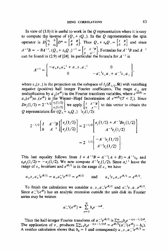
In view of (3.8) it is useful to work in the Q representation where it is easy to compute the inverse of (Q, + sQ J. In the Q representation the spin
operator is D[; z]D* = [i z]. Thus Q++ s,,Q-= [i :] and since
A-‘B = -BA-‘, (Q++ s,,Q-)-’ = . Formulas forA-‘B and A-’
can be found in (2.9) of [24]. In formula for A-’ is
A-’ = -a+s+a~’ + a-s-a:’ 0
0 -a;‘s+a++ al’s_a- I ,
where s+(s) is the projection on the subspace of I,(H ,,2, W) with vanishing negative (positive) half integer Fourier coefficients. The maps u,+ are multiplication by a +( eie) in the Fourier transform variables, where el”(‘) = a+(e’8)a -(eie) is the Wiener-Hopf factorization of e’*(‘)(T < T,). Since Dej(l/2) = 2-‘12 eJ(1’2) [e (,,*)I we apply [i :::I to this vector to obtain the
Q representation foi (Q, + sOQ J -‘ej( l/2):
This last equality follows from I + A - ‘I3 = A-‘( A + B) = A - ‘s, and sOej(1/2) = -ej(1/2). We now compute A-‘ej(1/2). Since CZ,” leave the range of s, invariant and eie12 is in the range of s, we have
a,s+a, e -1 i9/2 = a+a;leiB/2 = ei@/2 and -1 a+ w+e
it?/2 = eiO/2
To finish the calculation we consider a-s~a~‘e’~/~ and ~~‘s~a~e’~~~. Since a 5 ‘(eie) has an analytic extension outside the unit disk its Fourier series may be written
ayl(eie) = $ b,e-‘“@. n=cJ
Thus the half-integer Fourier transform of a 1 ‘eie12 is CF=,-,b,e - i(” - ‘12)‘. The application of s- produces Cz,= ,b,e - i(n - 1/W = ei@/2(azl(eia) - b,). A residue calculation shows that b, = 1 and consequently a -s _ a 1 ‘eie/’ =
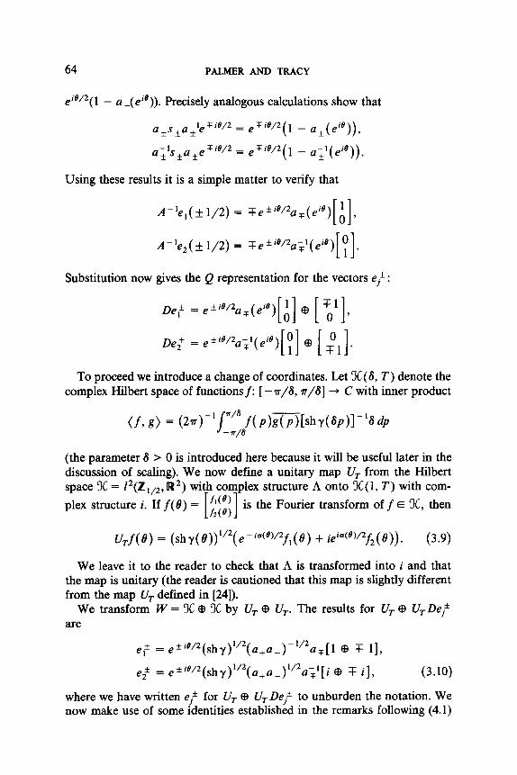
64 PALMER AND TRACY
eie/*(l - u - (e”)). Precisely analogous calculations show that
-I Tie/* _ a*s,a* e - erie/*(l - a,(eie)),
a;‘s,a,e Tie/* _ - eri@/*(l - a;l(ei@)).
Using these results it is a simple matter to verify that
A-‘e,( f l/2) = 7e*“/*ar(eie) A , [ 1 A-‘e,(+1/2) = ?e*ie/2u;‘(eie) y . [ 1
Substitution now gives the Q representation for the vectors ej* :
De,* = e +ie/2aT(eie)[A] cB [i,‘],
To proceed we introduce a change of coordinates. Let X (6, T) denote the complex Hilbert space of functions f: [ -n/6, r/S] --) C with inner product
(the parameter 8 > 0 is introduced here because it will be useful later in the discussion of scaling). We now define a unitary map U, from the Hilbert space X = 1*(Z ,,*, R*) with complex structure A onto X(1, T) with com- plex structure i. If f(e) = ;:I:; [ 1 is the Fourier transform off E X, then
U,f(d) = (shy(0))“2(e-iu(e)/2f,(t9) + iei”(“)/*f2(8)). (3.9)
We leave it to the reader to check that A is transformed into i and that the map is unitary (the reader is cautioned that this map is slightly different from the map Ur defined in [24]).
We transform W = X @ 3c by U, @ U,. The results for UT @ UTDej* are
* e1 = e*“/*(shY)“*(a+a-)- *‘*a,[1 GB T 11,
e2 * =e iie/2(shy)1’2(a+a-) “*a;‘[i 0 T i], (3.10)
where we have written ej* for UT @ UT Dej* to unburden the notation. We now make use of some identities established in the remarks following (4.1)
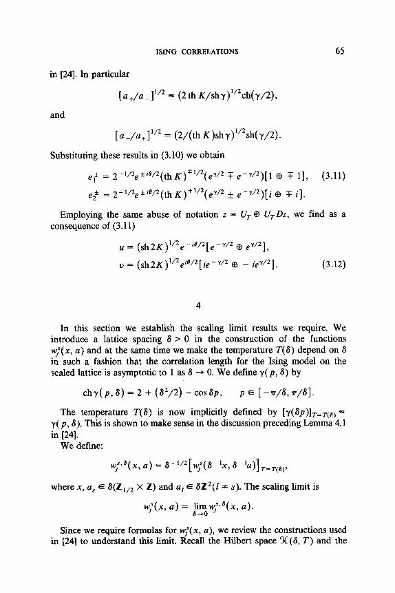
ISING CORRELATIONS 65
in [24]. In particular
and
[a+/~]“* = (2thK/shy)“*ch(y/2),
[u-/u+]“* = (2/(th K)shy)“*sh(y/2).
Substituting these results in (3.10) we obtain
e; = 2-‘/2efie/*(thK)~‘/*(e7/* T e-Y/*)[1 $ T 11, (3.11)
e: = 2-We*W*(th~) *“*(e7/* f eeY/*)[i $ T i].
Employing the same abuse of notation z = Ur Q UTDz, we find as a consequence of (3.11)
u = (sh2~)‘~*e-‘8/2[e-7/* @ eq
i) = (sh2K)1/2eie/*[ie-7/* $ - ied*]. (3.12)
4
In this section we establish the scaling limit results we require. We introduce a lattice spacing 6 > 0 in the construction of the functions wJ!(x, a) and at the same time we make the temperature T(S) depend on 6 in such a fashion that the correlation length for the Ising model on the scaled lattice is asymptotic to 1 as 6 + 0. We define y( p, S) by
chy(p, S) = 2 + (6*/2) - cosSp, P E [-e, @I.
The temperature T(6) is now implicitly defined by [y(6~)]r-r~~) = y( p, 8). This is shown to make sense in the discussion preceding Lemma 4.1 in [24].
We define:
w+“(x, u) = 6-‘/*[w;(6-‘x,6-‘u)]._T(B), J
where x, a, E 6(Z,,, x Z) and a, E SZ*(1* s). The scaling limit is
wJT(x, u) = frncw;p*(x, u).
Since we require formulas for w,!(x, a), we review the constructions used in [24] to understand this limit. Recall the Hilbert space X(6, T) and the

66 PALMER AND TRACY
unitary map U;. from X to X( 1, T) introduced in Section 2. The principal reason for introducing these coordinates is the simplifi~t~on which results for the kernels of A-’ and A-‘& In the following, we shall write M for A-‘BandNforA-‘.Define
M(f?, 6’) = i sh[tyW - ~(@‘%‘2f sin[(B + 8”)/2] ’
N(6,6’) = -i WYW + Yww~l sin[(B - 6’)/23 *
Then it is a consequence of 4.2 in [24] that the action of M and N in the X( 1, T) representation of X is
The integral defining N is understood in the principal vahxe sense (note: the map i f I
-y on X is transformed into the map which takes f( 8) to f( - 13 >
on X(1, T)). We introduce a unitary scale transformation from X (1, 2’) to X( S, 2’) by
f( 8) + f(&p)( p E [ - lr/6,lr/&]). Under similarity transformation by this scaling operator, the kernels of M and N become (relative to the measure t2~shy~~p))-‘~dp~
WP,P’) = i Sh[(Y@P) - Y@P’N/21 Sia%P + P’bQl ’
N(p, p’) = -i sh[frtW + r@~‘hd sin[a(p - p’)/2] ’
where ip 1 G rr/S and Ip’ 1 G T/S. To obtain the correct temperature dependence in the kernels for M and N
we define ~~~~~~~, p3 and N Ttsj(p, p’) to be the kernels M(p, p’) and N(p, p’> evaluated at T = T(6) (that is, y(6p) and y(6p’) are replaced by y(p, S) and yfp’, 8)). For s, t > 0 we let ~~(~~ denote the Schmidt class operator on X( 6) def = X(S, Z’(S)) with kernel e-S7(p*6)/8MTcaj(p, p’) e -sYfP’~8)/6. The action of M!,(s) on f E X(S) is obtained by integrating this kernel against f(p’)(Znsh y( p’, ii))-‘6 dp’ from -n/6 to n/8. For s, t > 0 fet &(s, I) denote the bounded operator on X(S) with kernel e -~~~~~~~~~~~~~~~p, pye -iyCP’,6)/6. The action of Ns(s, t) on fE X(S) is

ISING CORRELATIONS 67
given by integrating this kernel against f( p’)(2~ sh y( p’, 6)) - ‘8 dp’ from -T/S to a/S.
Let X(0) denote the Hilbert space of functions F: W --) C with complex structure i and inner product
(f, g> = $” f(P)g(p)(2sw(p))-‘dp, -CO
where w(p)* = 1 + p*. Define an isometric injection i,: X(S) + X(0) by
bf(p) = i8bMp)~ IPI Q r/a, = 0, IPI ’ w/s,
where i,(p) = (Sw(p)/shy(p, S))‘/*. Observe that ig: X(0) + X(S) is multiplication by x8( p)i,( p)-‘, where
X8(P) = 19 IPI G r/s, = 0, IPI ‘m/6’
Since lim 6+0a-‘shy(p, 6) = w(p), the space X(0) will provide a conve- nient arena for describing scaling results. Let s, t > 0. We define a Schmidt class operator M(s) and a bounded operator N(s, t) on X(0) by
Qw(J”)f(pt)(2aw(p’))-‘dp’.
The integral defining N(s, t) is understood in the principal value sense. The significance of these operators is that i,$&(s)i~ converges in Schmidt norm to M(s) as S + 0, and the difference xJV(s, t)xs - i&(s, t)ig converges to zero in operator norm as S + 0 (see Lemmas (4.2) and (4.3) in [24]). Before we state our principal result on scaling, it will be convenient to introduce some further terminology. Let W(S) = x(S) CI!J X(S) and W(0) = X(0) $ X(0). The reader should note that the complex structure on these spaces relative to which F( *) is linear, is i d (-i). Let
Q&,, E2) = Q+,-W(P.8)/6 + Q-,-Wh8)/6
and
Q(&,, e2) = Q+e- W’(P) + Q e-W’(P)a -
We will say a measurable function f: W -+ C* is (E,, E*) almost in W(0) if
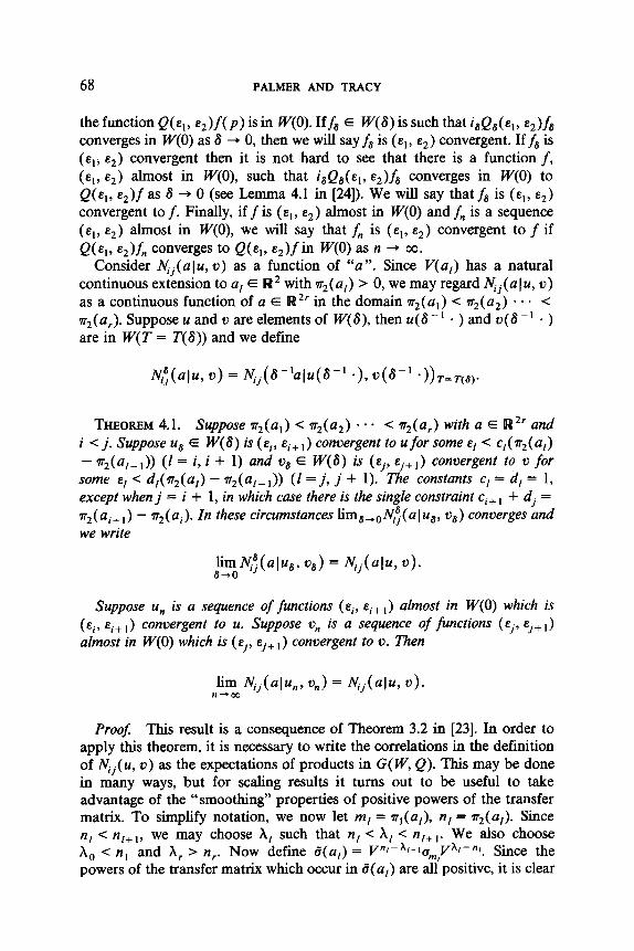
68 PALMER AND TRACY
the function Q( e,, eZ)f( p) is in W(0). If fs E W( 8) is such that isQs( E,, E*)& converges in W(0) as 6 + 0, then we will say fs is (E,, E*) convergent. If fs is (E,, e2) convergent then it is not hard to see that there is a function f, (E,, e2) almost in W(O), such that isQg(e,, eZ)fs converges in W(0) to Q(E,, e2)f as 6 + 0 (see Lemma 4.1 in [24]). We will say that f8 is (E,, Ed) convergent to f. Finally, if f is (E,, a*) almost in W(0) and f, is a sequence (E,, Ed) almost in W(O), we will say that f, is (E,, E*) convergent to f if Q(E,, eZ)fn converges to Q(e,, eZ)f in W(0) as n * co.
Consider Nij(a] U, u) as a function of “u “. Since V(a,) has a natural continuous extension to a, E W 2 with v2( a,) > 0, we may regard Ni j( a ] U, V) as a continuous function of a E W2’ in the domain rr2(u,) < g2(u2) . . . < rr2(ur). Suppose u and v are elements of W(S), then ~(6~’ . ) and v(S-’ . ) are in W( T = T( 8)) and we define
A$(ulu, u) = ~j(6-‘ulu(6-’ *>, u(S-’ ‘&-T(6).
THEOREM 4.1. suppose r2(ul) < r2(u2) . . + < r2(ur) with a E R2’ and i <j. Suppose ua E W(6) is(Ei, ei+,) convergent to uforsome E, < c,(9r2(u,) - ~T~(u,-~)) (I = i, i + 1) and u, E W(S) is (ej, ej+,) convergent to u for some E, < d,(lr,(u,) - T~(u,-,)) (I =j, j + 1). The constants c, = d, = 1, except when j = i + 1, in which cuse there is the single constraint ci+ , + dj = r2(ui+ ,) - r2(ui). In these circumstances lim 8+,,l$(ulub, ug) converges and we write
limA$(ulu,, ug) = Nii(u]u, u). 6-O
Suppose u, is u sequence of functions (q, q+ ,) almost in W(0) which is (q, q+,) convergent to u. Suppose u, is u sequence of functions (ej, Ed+ ,) almost in W(0) which is (ej, Ed+,) convergent to u. Then
lim A$j(a]u,, n-+ca
u,) = Nij(UJU, u).
Proof: This result is a consequence of Theorem 3.2 in [23]. In order to apply this theorem, it is necessary to write the correlations in the definition of Nij(u, u) as the expectations of products in G(W, Q). This may be done in many ways, but for scaling results it turns out to be useful to take advantage of the “smoothing” properties of positive powers of the transfer matrix. To simplify notation, we now let m, = ~,(a,), n, = 7r2(u,). Since 4 < n1+1, we may choose A, such that n, < A, < n,, ,. We also choose A, <n, and A, > n,. Now define B(u,) = Vn’-hl-lu Vhlmn’. Since the powers of the transfer matrix which occur in B(u,) are 3 positive, it is clear

ISING CORRELATIONS 69
that d(a,) E G(W, Q). We introduce
~(6, u,) = T(I~I,,O)(Q+T”‘-~‘-’ + Q-F-“+,(S-’ -),
~(6, a,) = T(m,,O)(Q+T”~-“l-1 + Q-F-*+,(6-’ -). (4.3)
It is now an elementary calculation that
(4.4)
where b, = S - ‘a, and i * j. The case i = j is analogous. For brevity, we mainly confine our attention to i * j. Theorem 3.2 in [23] applies directly to (4.4) with g, = a( 6 - ‘a,). The formula for the right-hand side of (4.4) which we shall present is based on Hilbert space constructions on the space W(T = T(6)). Since we wish to work in W( 8) we will make the unitary scale transformation in these constructs as they are introduced rather than repeat the formulas. The operators L( g,) and AR( g,) in Theorem (3.2) of [23] are easily computed. Their action on W(6) is
I x&r - b, A, - 4 0
L,k,) = 0
I x,,'(n, - A,-,, A, - q> '
[
0 AR,(&) =
-%n,*b, - h,)
wn,&I - n,) 0 I 9 (4.5)
where X,,(s) = e”“pX,(s)e- imp Let IV(S) denote the direct sum of r . copies of W(8). Define AR, to be the r x r block diagonal matrix on IV(S) with entries (AR,)ij = SijAR8(gi), and define L, to be the r x r block matrix on IV(S) with entries
LiT’ = -Q+L,(gi+,) *** La(gj-,), j>i+l,
= -Q+, j=i+ 1, =
= :-, j = i, (4.6 ) j=i-1 7
= Q-Li’(gi-1) *** Li’(gj+l), j<i-1.
Now let u6( a,) and ua( uj) denote the elements of W( 6) given by the unitary scale transforms of u(S,6-‘a,) and ~(6, a-‘~~). The formula for the

70 PALMER AND TRACY
right-hand side of (4.4) as given by Theorem 3.2 in [23] is
where & is the injection of IV(S) into the ith slot in W’(S), the conjugation *I @ u2 = u2 $ U, (on W(6)), and the inner product is the standard Hermi- tian symmetric one on W’(6). The operator I + L,AR, is shown to be invertible in 1241.
We now use the isometric injection i, to transform the inner product in (4.6) into an inner product on W’(0). The argument in Theorem 4.2 of [24] then shows that is{ I+ L,AR,) -‘L&j converges strongly to the operator on ?V(O), which one obtains by replacing M,(s) and N,(s, t) in (4.4) by M(s) and N(s, t). We write L and AR for the operators on W’(O), which are obtained from I;, and AR, by such substitution. We now note that the exponential factors in the transfer matrix in (4.3) and the fact that us and oa are (E,, a,+ ,) convergent are enough to guarantee that isus and isus do converge in W(0). The idea is that the intermediate points A, may be chosen arbitrarily with one exception. That exception is Xi whenj = i + 1. In this event, (nj - A,-,) + (Xi - ni) = n,+i - n, is a constraint. The hypothesis ci+, + dj = n,, , - ni ensures the convergence of isus and isus for the appropriate choice of hi between ni and n,+,. We write ui(p) = eimJ’Q(ni - Ai-,, Ai - ni)u(p) and t+(p) = eimiPQ(nj - Aj-i, hj - nj)u( p) for the limits of i,u,(a,) and isus( We have demonstrated
lilh#;(alu,, ud) = -((I + LA@-‘Ll&), Ii(q)). (4.8)
The exponentials e -‘@, which relate ui and vi to u and u, make it quite clear that the limiting functional on the right-hand side of (4.8) is continu- ous relative to (E,, E!+ i) convergence in u and u. This finishes the proof of Theorem 4.1. U
We are now prepared to consider the scaling limit of M$~‘(x, a). Let wjLts(x) E lV(6) and ud E W(6) denote the scale transforms of S - i/2 wj* ( X, S) and o( (see Section 3.3 and 3.5). Consulting Theorem 3.1 we find that for 1 < s:
wjqx, u) = NISs(,Ily&(X - u,), us), n,-, 6 x2 < n,,
w;qx, u) = N;(aJw)yx - a,), us), n, G x2 d n/+1.
According to (3.12), us(p) = (sh2K)‘/*e-‘@“*[e -YfP,s)‘2 gr eY(Py’)fl]. Recalling Lemma 4.1 of [24] it is evident that ug is (E, E) convergent to 1 CB 1 for any E > 0.

ISING CORRELATIONS 71
In order to apply Theorem 4.1 we must show that wiF8(x - a,) is (n, - A,-,, A, - n,) convergent as 6 --) 0. The vector Qs(n, - A,-,, A, - n,)wjr8(x - a,) is given by
Xl, 42 [ 1 0 x** f/,6(X - 4 where
x,, = ,&%I - dY(PT Q/S >
x,, = ,(h/-l-n/)Y(P,6)/6M~,
x2, = e(“/-b)7(P3wQJ8,
fj,dy) = e iY1PQs(~2, -Yz)[gj,a 8 gj,s]T
and
(4.9)
&,6(P) = (26) -‘/‘(&,,( p, a))‘/“( jeia(P,S)/2 - e -ia(p,a)/2),
g-,,*(P) = (W -1/2(shY(P, a))‘/2(ieidP.a)/2 + e-‘Q(P.6)/2)e
If we suppose A,-, < x2 < n,, then the convergence results for M,(S) and &(s, t) noted earlier in this section show that to settle the (n, - A ,- ,, A, - nl) convergence of wjy8(x - a,) it suffices to prove the (E, E) convergence of gj: 6 @ gj, 6 for any E > 0. The reader should observe that if x2 is in the open interval in (n, _ ,, n,), then A,-, may always be chosen so that A,-, < x2 since the (E, E) convergence of the vector u8 imposes no constraint on the choice of intermediate points A,. It is a simple calculation to show that lim s+06-‘shy(P, 8)eia(‘p) = 1 + ip. Furthermore, Lemma 4.1 of [24] shows that this convergence is dominated in such a fashion as to imply the (E, E) convergence of gj, 6 @ gj, s. The limits gj( p) = lims,ogj, s(p) are then easily computed using the fact that the square root, ,/m, which arises in this computation is given by 2-‘/2(5’/2ein’4 + 5 - ‘12e - i11’4), where 5 = p + I/%. The results are
g,(p) = -tlPe-ilr/4,
g-,(p) = ,t-‘/2ei”/4.
We have assembled enough information to show that Theorem 4.1 applies to the convergence of w,!’ ‘(x, a) for n,- 1 -C x2 < n,. We have also shown the reader how to obtain the scaling limit analogue of Theorem 3.1. Before we state such a result, it is useful at this point to make a systematic introduction of the mass shell coordinate ,$ = p + /g. Under this

72 PALMER AND TRACY
change of coordinates, the complex functions square integrable on BP with respect to (2770(p))-‘dp are mapped umtarily onto the space of complex functions on (0, oo) square integrable with respect to (2~0 -’ d<. The kernels i(o(p) - w(p’))/(p + p’) and -i(w(p) - w(p’))/(p -p’) be- come in the new coordinates i(< - .$‘)/([ + 5’) and - i(t + <‘)/(< - t’). The following theorem is the scaling analog of Theorem 3.1. To avoid introducing more notation, we write Nii (~1) u, u) for the function introduced in Theorem 4.1, and w,?(x, a) will now denote the scaled wave function.
THEOREM 4.2. Suppose ~~(a,) < q(u2) . e .
(1) ifl<s
yqx, a> = N,,(alw,-(x - q), u),
$(x9 4 = N,,(ulw,t(x - a,), u),
(2) if I = s
wi”(x, 4 = Nss(ulw,-(x - a,), u),
+ (T(x - u,)Q-4, ii>
wi”(& 4 = N,,(alw,f(x - a,), u),
- (T(x - u,)Q+& 8; (3) if 1 > s
wi”(x, u) = -N,l(ulu, y-(x - a,)),
wi”(x, u) = -N,,(ulu, wi’(x - a,)),
< v2(u,), then
n,-, < x2 < n,,
We write wj*(y) = wj*(r, cp), y = r(cos cp, sin cp). The functions wj*(r, cp) in muss shell coordinates 5 are
(y-(r, cp)), = e- (r/2Xt(r)+~t~)-‘)gi(5)
+i /
*5--t’ -,r~,2Xr,c~)+~‘~)-l)~~, 0 5+5’
(bvP(r,(p))2 = -ijgwfie -(1/Z)(6,(-r)+~,(-.)-l)~~(~~)~,
(wT(r, cp)), = -ijom~e-(r/2)((.(r)+l’(~)-‘)~j(~~)~, (4.10)
($(r, cp>), = e- (r/2)(~(-cp)+c(-cp)-‘)gj(5)

ISING CORRELATIONS 73
where 5((p) = -ie’q[, g,(t) = -e-i”‘4[‘/2, g-,(t) = ein’4(-1/2 UTZ~ the inner products are
where x - a, = r,(cos ‘p,, sin(p,). We now scale the difference identities in Theorem 3.2 to obtain formulas
for the derivatives of scaled n-point functions. Suppose r2( a,) < vr2( u2) . . . < ~~(a,), then we write
T(6)’
(u(a)> = fyJ*bh (4.12)
(U”(U)) = ~L_mg(u;qu)).
For collections of sites {a,} with noncoincident second coordinates, the convergence of these limits was established in [24]. We now require more detailed information about this convergence. Suppose a, (I * i) are consid- ered fixed, and ai is permitted to range over a compact region Ci with the second coordinates of Ci strictly between r2(aieI) and 7r2(ai+ ,). Let a,(k) = ~~(a~). The result we require is that ~(t~~(a))/~a~(k) and a(ugqa))/aai(k) converge to a(u(a))/8ai(k) and ~(u’j(a))~a,(k) uni- formly for a, E Ci as 6 + 0. We sketch how to obtain such a result for a( u8( a))/&~( k) (the other case may be treated analogously). In [24] it was shown that (us(a)) = det,(Z + G,(a)) (where G&(u) = L,AR,) and the convergence in (4.12) was proved by demonstrating that isGGi;f converged in Schmidt norm to a Schmidt class operator G(a). Using Lemmas 4.1-4.3 in [24] it is not hard to see that the difference quotients for Gs(a) in ai converge to 8G6(a)/dai(k) in Schmidt norm. Differentiating det,( .) one finds
~(u~(a))/&z,(k) = -det,(Z + G6(u))
xTr(G,(a)(Z + G&(u))-‘aG,(a)/aai(k)).
Pointwise, convergence to 8(u(a))/8ai(k) as 6 + 0 is an immediate conse-

74 PALMER AND TRACY
quence of the convergence of isdG8(a)/c?ai(k)i~ to aG(a)/Q(k) in Schmidt norm, and it is not hard to make the estimates for the convergence uniform provided the differences rl( a,) - rl( al _, ) are uniformly bounded away from zero. The essential point is that differentiating G,(u) with respect to ai brings down factors, ip or - y( p, S)/6, which always occur in conjunction with, and are controlled by, the presence of factors e -(n~-n~-lh(~*S)/S (see Lemma 4.1 of [24]).
The uniform convergence of the derivatives has the following useful consequence, which for clarity we state for functions of a single real variable “a.” Supposefi( a) is continuous and converges locally uniformly to f’( a) as 6 + 0. Then 6 - ‘( fs( a + 8) - fs(u)) converges to f’(u) as S + 0. The proof is an elementary consequence of the mean value theorem. This simple observation coupled with Theorem 3.2 and Theorem 4.1 yields the following result:
THEOREM 4.3. Suppose ~*(a,) -c . . . < vr2(ur). Then
(l) ~a(u)~~‘a(a(u))/aui(l) = -%j(-w(P) @ O(P), l @ I), (2) (a(u))-‘~(o(u))/&z,(2) = -&(-p @p, 1 @ l), (3) (a(u))-l~(ai~(u))/&xj(l) = -i&.j(-p $ p, 1 $ l), i <j,
(4) (u(u))-‘a(uiqu))/aui(2) = -jyj(-w(p) CD w(p), 1 @ l), i -c j.
Proof. The proof is a simple scaling calculation and is left to the reader. It is helpful for this calculation to replace u(iu) in (3) of Theorem 3.2 by u( u + iv) before proceeding. One should also remember that X(x) = F(i @ (- i)x). The continuity result (4.1) makes it straightforward to justify the limits which are encountered. 0
5
In this section we show that is a multivalued solution of the
Euclidean Dirac equation with ranch points at a, (I = 1,. . . , r), and we compute local expansion coefficients for these solutions at the branch points. The Euclidean Dirac equation satisfied by WJ(X, a) is
[
-1 a/ax, - it?/&, a/ax, + is/ax, -1 ][ J$yy = [;I. (5.1)
It is easy to prove this when x2 is strictly between n, and n,, ,. Consulting
Theorem 4.2 it is enough to show that Wlf(r’ ‘) [ 1 w-+,(r. ‘p) is a vector valued solution

ISING CORRELATIONS 75
of (5.1). For this purpose it is convenient to introduce x = (1/2)(x, f ixz) and replace e -(r/2)(~(‘T)+f(‘T’-‘) with eitX-it-‘z, ad so on. The differential operators 8/8x, f id/ax, acting on such exponentials bring down factors it and (it) -’ which convert g- ,([) into g,(5) and vice versa. In each case
this is all that is needed to show that W’(r’ ‘) 1 I
is a vector valued solution w_:(r, cp)
of (5.1). We remind the reader that the complex structure in the differential operators a/ax, f is/ax, acts in W(0) as i cl3 (-i).
We next present arguments to show that the different expressions for wf(x,a) [ 1 wS,(x,a) piece together to give a solution to the Dirac equation every-
where except on the horizontal rays to the right of the branch points a,. On these rays the upper and lower limits differ by a sign. In order to show that the function +4(s, n) [ 1 wsl(x,n)
satisfies the Dirac equation on the rays to the left of
the branch points a, it is enough to show that it is continuous on these rays, Once continuity is established a straightforward integration by parts shows
that wf(x, 0) [ I wS,(x,n)
is a local distribution solution of (5.1). Elliptic regularity
then implies it is actually a Cm solution. We turn next to the continuity and monodromy properties for w,?(x, a).
Theorem 4.1 shows that to prove these results (for a, (1 * s)) it is enough to show that
lim w~+(T, ‘p) = l&r+ wj-(r, cp), ‘p-IT-
lim wj+(r,cp) = - lim y-(r,(p), (p-04 p-*29?-
(5.2)
where the convergence is (E,, Ed+ ,) convergence in W(0). When Q, = a, one needs in addition the appropriate boundary values for the inner products P-(x - a,>Q,& ii>. S ince these inner products are simple to deal with we consider them first. In the integral
introduce the complex integration variable z = - [( cp,) and then deform the contour of integration to the positive real axis. The result is

76 PALMER AND TRACY
Introducing z = ~(cP,) in the integral
and deforming the contour to the positive real axis one obtains
mx - a,)Q+f,, ii> = -&/2 J me-(r,/2)(r+r-‘)Z1/2~ 0 2rz ’
0% - a,)Q+f+ ii> = ei*p,/2 (5.4
Recalling Theorem 4.2, it is evident that these inner products have the appropriate ~nt~~ty and mon~romy. In order to prove the con~uity results (5.2), it is convenient to transform the expressions for wj*(r, (p). In each of the integrals in (4.10), introduce the complex change of coordinates z = rt E( + cp). The choice of z is made so that in each case e -(r’2Xz+r-‘) appears in the integrand. Now rotate the integration contour to the positive real axis. The integrals containing the principal value kernel
will pick up contributions from poles under this change of contours. (Except, of course, when no rotation of contour is needed at cp = IT/~, 31r/2). One finds
(wf(r, cp)), = -e-‘~/2~(cp)‘/2e-(r/2XC(cp)+~(~)-’)
-,-b/2 s
WZ- iei’lz1,2e-(r,2)(z+r-l) dz 0 z + ie”[ 2112’
+ ieW2 I
cm z - ie-b(
0 z + iemiT
z*,2e-fr/2K~+~-‘)&
(w_fi(r, q)), = ei’/2E(cp)-‘/2e-(r/2)(~(cp)+~(~)-’) (5.5)
+ ie iV/2
/
00 z _ ieM< dz 0 z + ieiqt
z-l/2e-(r/2Xt+r-‘)~
2nz ’

ISING CORRELATIONS 77
and
- ie - iP/2 J
mz-ie -ipSZ-1,2e-(r/2)(r+r~‘)dZ
0 z+ ie-“P( 2at ’
where the square roots E( + cp) * ‘I2 are all computed by taking arg t( f cp) E (0,2a). The continuity and monodromy results (5.2) are immediate conse- quences of (5.5) and this square root convention. The reader should note that [( f (p)‘12 is discontinuous at cp = r/2, 3~/2 (not at cp = 7rIT, 2s). At these points the formulas in (5.5) are not correct; the singular integrals which occur should be interpreted in the principal value sense and the “pole terms” associated with these integrals should be dropped.
We are now prepared to compute the coefficients in the local expansions of $(x, a). Define
e,(cp, n) = (eitn-‘12) (p,O), e,(cp, fl) = (0, eicn+1/2)y),
and
Here I,(r) is the modified Bessel function of order Y. A contour integral representation of I,(r) which is particularly useful for our purposes is
l”Jr) = e’(Y+‘)” 1
s-Ye-w2w-i&,
C
where the contour C starts at + oc on the positive real axis just in the lower half plane, winds clockwise around the origin, and finishes at + oe on the positive real axis just in the upper half plane.
It is shown in [26] that a two valued solution, f(x), of the Euclidean Dirac equation with a branch point at x = a has an expansion
f(x)= E [c(n,+)u(r,cp,n)+c(n,-)~(r,cp,n)l, (5.6) n=-CC
where (x - a) = (r cos cp, r sin cp), cp E [0,2n). Our goal is to calculate the coefficients c;(n, &)(wS(x, a), wS,(x, a)) about each branch point a,. In particular, we will show that c;(n, +) = 0 for n < 0. This will have conse- quences for the order of growth at the singularities a, and is an important part of the SMJ analysis. The reader should have no trouble seeing that the

78 PALMER AND TRACY
calculation of the coefficients c,S(n, &) reduces to the calculation of half- integer Fourier coefficients for the vector valued functions wj*(ri, q,) and the inner products (T(x - u,)Q *fi, 2). The Fourier coefficients for these inner products are obvious from Eqs. (5.3) and (5.4), and the other Fourier coefficients in question are
fjk = &lr(eikq cl3 emikq)Wj+(r, q) drp
+ &1,2’(eixp 8 eeikq)wj-(r, cp) dcp, (5.7)
where k E b,,2. The factor ei“q @ e - ikp appears because Z(x) = F( i @ (- i)x). In order to calculate the Fourier coefficients it is useful to work with the representation for wj*(r, cp) in (5.5). Perhaps the simplest way to extract the Fourier coefficients from the integrals is to use the geometric series expansions:
3 = 1 + 2 2 (-;5)nx-., 5 < x, n=l
X-E- - - x+E 1 2 E (-<)+xn, 5 2 x. n=l
Once this is done and the other cp integrals are converted to contour integrals on. the circle (zl = 5, the z integrals which result are naturally contour integrals over two sorts of contours:
The first contour is immediately identifiable as a Bessel function; the second contour may be deformed to the unit circle and subjected to the change of variable z + z-‘, at which point it, too, is evidently a Bessel function. The result of these calculations are
flk = Ik(r) -i(i’)-” [ I i(g-”
, k = n + l/2, n = 1,2,. . . ,
y k = l/2,
= I- k(r) -i(i<)”
I I i(it)” ’ k = -(n - l/2), n = 1,2 ,...,

ISING CORRELATIONS 79
f*k = Ik(T) 4W” [ I i(g)-”
) k = n - l/2, n = 1,2,. . . ,
k = - l/2,
= I-Jr) -i(i[)” i I i(i[)” ’ k = -(n + 1/2),n = 1,2, . . . .
We may use these results to calculate the coefficients cf( n, f ). Before we record the results, it is convenient to make a number of observations. In order to calculate ci(O, ZL ), it is useful to note that
J m,*l/2e-(r/2)(z+z-‘) dz - 1 1
0 zaz 2 ( -1,2(r) -4,2(r)).
The operator X = (I + LAR) - ‘L which appears in (4.8) is P skew-sym- metric. That is PX*P = -X. This follows directly from the fact that L and AR are both P-skew symmetric, a fact which is easily verified. One conse- quence of the P-skew symmetry of X is that N,,(u, u) = 0. The reader should note that because NS,(u, U) = 0, the coefficients c,“(O, +) are de- termined completely by contributions from the integrals (5.3) and (5.4).
Finally, if we introduce the notation 8/&z, = 6’/8a,(l) - i~?/&~(2) and a/@ = a/au,(l) + ia/aa,(2) then the results of Theorem (4.3) may be summarized
(5 *9>
Here we use the conventions u = 1 @ 1 and
(i[)“u = (it)” @ (it)“.
We are now prepared to state the main result of this paper:
THEOREM 5.1. Suppose 7r2(u,) < 7r2(u2) .a. < ~~(a,). Then the scaled Euclidean wavefunctions w,?(x, a) satisfy the Diruc equation (5.1), except on the horizontal rays to the right of the points a, where they have upper and lower boundary values differing by a sign. The expansion coefficients cf( n, *) in the

80 PALMER AND TRACY
expansion (5.6) are given by
c;(n, +) = 0, n < 0,
4(0, k> = +S,,/2 - (eSi/2)iV,,(alu, u), &S = , (
+1 I<s -1 I>s’
cf(n, *) = -e~iN,S(aI(i~)“u, u), n = 1,2 ) . . . .
The coefficients cs( 1, f ) may be expressed in terms of derivatives of scaled n-point functions as follows:
c,“(l, +> = (u(a)>-‘J(u(a)>/%,
c,“(l, -) = - (u(a))-‘f3(u(a))/~~S,
cf(l, +) = -ie;(u(a))-‘a(u’“(a))/Ja,, 1 f s,
cs(l, -) = -ie~(a(a))-‘8(a’S(a))/&7,, I f s.
The functions w,T(x, a) are exponentially small as 1x1 + m.
Proof: The only part of this theorem which is not a direct consequence of Theorem 4.2 and Pqs. (5.6), (5.8), and (5.9) is the very last statement of the theorem.
In order to prove that the functions yT(x, a) are exponentially small for x near infinity, it suffices to show that these functions are bounded for 1x1 sufficiently large (see Proposition 3.1.5 in SMJ [26]). In view of the represen- tation for yf(x, a) in Theorem 4.2, we seek bounds for Nls(wj*(x - a,), u), Nsr(u, y*(x - a,)), and (T(x - a,)Q& ii> for x in an appropriate region. The expressions (5.3) and (5.4) for the inner products (T(x - a,)Q& E) are exponentially small for large values of Ix - a, ] so that we may concentrate on the other terms.
First consider N,s(y-(x - a,), u) for 1 = 2,3,. . . , r. Choose ek (k = 1 ,‘.., r ) as in Theorem 4.1. Since e -EW~ is in X for arbitrarily small E > 0, we may choose E, subject only to the inequality E, < ?r,(a, - a,- l). We will establish a bound on Nls(wj-(x - a,), u) for x in the strip r*(a,) - et G x2 G rz(a,) with Jx - a,J sufficiently large. Since N,s(wj-(x - a,), u) depends linearly on y-(x - a,), the continuity result in Theorem 4.1 shows that we need only bound the norm of Q(E,, E,+ r)wj-(X - a,) in W(0). For this purpose the representation in (5.5) for wj-(x - a,) is useful. Let x - a, = (r,cos ‘p,, r,sin cp,) and recall 2w = 6 + 5 -‘. Making use of the inequality
z - ie+E
2 + ie+t d/~=tan~+secpl, cpE[n,27r],
and (5.5), one easily finds that the absolute value of the function
ISING CORRELATIONS 81
eUe““Q+wj-(x - a,) oft is dominated by
+ (tancp, + seccpr)e-r~(~+tm’)‘2j z m j/2e - r,(z+Z-')/2-
0 Ez. (5.10)
The nom of [j/ze -(X2 - nz(W)+e,XE+6-‘)/2 in X is uniformly bounded, pro- vided x2 - ~,(a,) + E, 2 E > 0. On the other hand, if we restrict ‘p, to the union of the intervals [n, 5s/4] and [7n/4,2s], and take r, > 1, then tancp,+seccp,-=&nd
/
dz 00zj/2e-(rr/2)(~+~-‘)- < 0 /
mzj/2e -(r+z-‘j/2- dz 2nz 0 2sz *
It follows that the norm in X of the second term on the right-hand side of (5.10) is uniformly bounded for x in the region determined by ‘p, E [n, 57r/?r] U [7a/4, 27r] with r, 2 1. Now consider the function e - E’+ ‘“Q _ wj-( x - a,). Making use of the inequality
and consulting (5.5), one sees that the function e - E’+l“Q _ wj-(x - a,) is dominated by
+ (seccp, - tancp,)e-EI+I(E+I-‘)‘2 J
mZj/2e-r,(z+z-1)/2&
0 2vz * (5.11)
If we again require that ‘p, E [v, 577/4] U [77r/4,2s] and r, 3 1, then it is clear that the norm of (5.11) in X is uniformly bounded. It is evident that precisely the same considerations bound NJu, wj-(x - a,)). Putting these results together we conclude that the function w;(x, a) is uniformly bounded in the strip ~~(a,) - E, G x2 G ITS with (x - a,1 sufficiently large, 1 = 2,3,. . . ) r, and E/ < ~,(a, - a[-,).
If we now consider the representation of the functions w;(x, a) in terms of N,,(w,+(x - a,), u) and NJu, wj’(x - a,)), then the same estimates on (5.5) show that w,!(x, a) is uniformly bounded in the strips v2(u,) Q x2 < v2(u,) + E,+, for Ix - a,] sufficiently large, I = 1,2,. . ., r - 1, and a,+, -C vr2( a,, , - a,). Putting these results together we conclude that the function w,!(x, a) is uniformly bounded for all x such that v2(u,) G x2 < vr2(ur) with lx] sufficiently large. Thus we concentrate further attention on the cases
82 PALMER AND TRACY
x2 < ~~(a,) and x2 & ~~(a,). For x2 < ~~(a,) the function wjs(x, a) is given by 4s(wj-fx - a’), u). In this formula wj-(x - a’) may be replaced by Q-y-(x-a,). Thi s o f 11 ows from the formula (4.8) for N,Ju, u), but may also be understood in the following manner. Before the scaling limit is taken, the operator $j(x)o(a,) (or Jjj(~)p(a,)) occurs in the vacuum expectation defining W.J(X, a) for x2 Q ~z(u’). When #Jx)a(u’) (or +Jx)~(a,)) is expressed as a normal ordered product as in (3.4) or (3.6) the function Q+?-(x - a’) appears in a creation operator to the left of all the spin operators. The adjoint of this operator acting on the vacuum gives 0. Thus only Q-T-(X - a,) makes a nontrivial contribution to the lattice wave function. Of course, this will persist in the scaling limit. We are thus reduced to proving that e - “‘“Q -wj-(x - a,) is uniformly bounded in X norm for x2 G ~r,(u’> and Ix - Q’ 1 sufficiently large. For the region cp, E [n, 5n,‘4] u [7?r/4,2 ] v an r, 2 1 the estimates given above suffice. For the d region cp’ E (5n/4,77r/4) and r’ & 1, it is useful to employ the representa- tion (4.10) for Q-VVJ(X - a’). As a function of 5, the vector e - ew ’ Q-wj-(x - aI) is given by
e-e,(t+E-‘)/2 $
* 5 + 5’ o -E;.(F) de’, (5.12)
where q(t) = (27ri&-‘gj(l)e- r,(f(-Pl)+t(-fPl)-‘)m S&-e (6 + [‘)/(t - 5’) = (25/(5‘ - c’) - 1, it follows that the function in (5.12) is
e-Ei(E+f-‘)/2 20 ( iwgdt’ - e-ef(C+f-‘)/2~mJj(C’) d<‘. (5.13)
Since Il$(()I 6 (2~E)-‘Ej/2e-‘I(I+~-‘)/2~ for q, E (57r/4,77r/4), it fol- lows that the second term in (5.13) is uniformly bounded in X norm for ‘p, E (5n/4,7n/4) and r, & 1. Now let Gi([) = Jo”{ F( .$‘)/(5 - 5’) dt’. Then the square of the X norm of the first term in (5.13) is given by
An elementary application of calculus shows that
te-et(E+t-‘) 6 (2e,)-‘( 1 f Ji-+G$)e-W.
(5.14)
Using this, and the fact that the truncated Hilbert transform is bounded on L2(d[), it follows that the norm in X of the first, term in (5.13) is bounded by a constant times the L2(d&) norm of q(S). The estimate of Fj(t) above shows that this norm is uniformly bounded in the region cp, E [5+7/4,713/4]

ISING CORRELATIONS 83
with r, z 1. When x2 >, ~~(a~), one may deal with Q+w,‘(x - a,) in.an analogous fashion. This completes the proof of Theorem 5.1. •I
6
In this section, we review the SMJ analysis of monodromy preserving deformations of the Euclidean Dirac equation and its application to the Ising correlations. Let yz = P 0’ and y, = [y i]. The Euclidean Dirac [ 1 equation is
i a a
Y2a,2 + ylax, -in w=o, 1
(6 -0)
where w = (w,, w- ,) E C2. We are interested in spaces of multivalued solutions to this equation with isolated singularities aj E lR2 ( j = 1,. . . , r) and specified monodromy at each point aj. It is convenient to introduce complex coordinates z = 1/2(x, + ix,), f = 1/2(x, - ix2) and differential operators a = a/ax, - id/ax, and a = a/ax, + id/ax,. We also write
[
a,(l) + iad2)
A = (l/2)
0 ‘.:,l)“,,,,l and L= [ 1 ‘** 1-j’
wherelj(j= l,..., r) are real numbers, and we will use the notation
aj = a/au,(i)- ia/aa,(2), 4 = a/aaj(i>+ id/s,(2),
&tj = (1/2)(daj(l) + idaj(2)), and
u5$ = (1/2)(daj(l) - idaj(2)).
Let Rj(r3) denote the rotation by 8 about aj; that is
Rj@)X = aj + R(Q(x - Uj)) where R(B) = [y; -y. cos e
DEFINITION. W( L, A) will denote the complex linear space of multival- ued solutions w to (6.0) with isolated singularities at aj (j = 1,. . . , r) satisfying:
1) w(Rj(2n - )x) = e 2n(~-1/2)i~(~) for x near aj,
2) jR2(W,R, + w-p-,) dx < 03.
Because of the monodromy condition, the functions w&( k = f 1) are single valued on W2 and the integral in 2) is well defined. The monodromy

84 PALMER AND TRACY
condition fixes Ii mod Z and our convention will be to choose each lj so that - l/2 < $ < l/2.
Before we present any more details, we will outline the main features of the analysis in [26].
First the space W(L, A) is shown to be finite dimensional with dim W( L, A) = r, where - l/2 < $ c l/2 ( j = 1,. . . , r ). A “canonical” basis ( Wj}J- , is constructed which spans W(L, A). Because W(L, A) is finite dimensional and because there is a natural action of infinitesimal rotations on the IV, it turns out that the Euclidean Dirac equation for each Wj may be extended to a holonomic system:
d,,,W’ = i i-i$jWk, (6.0 k=l
where the Q$) are one forms in dz and dZ with coefficients that are unknown functions of A, hwith explicit dependence on t, Z. Next, one supposes that the “canonical” basis Wj depends differentiably on the points aj away from places of coincidence aj = ak ( j * k). Again using the finite dimensionality of W( L, A) one sees that dA, A -Wj may be expressed as a linear combination of 8Wk, gWk and Wk (k = 1,. . . , r) with coefficients that depend on A, x However, because of (6.1) the z and f derivatives of Wk are linear combina- tions of Wj(j = l,..., r). Thus one has
(6.2)
where Gjj’s are one forms in dA,, a%$ with coefficients that are unknown functions of A, x that depend on I, Z in an explicit fashion. Combining (6.1) and (6.2) one has
d,,,,,,,-Wi = i i-ijkwk,
k=‘l (6.3)
where Q = P(‘) + SIc2). The consistency condition for this holonomic system is
(6.4)
Thus one may expect that the coefficients in the matrix valued one form SI satisfy nonlinear differential equations. The assumption concerning the differentiability of Wj ( j = 1,. . . , r) in the variables A, x is disposed of in the following manner. First choose A, without coincident entries. Then construct the canonical basis Wj(z, z; A,, &) for W(L, A,). Using (6.1) this determines SIC’) at A,, &. The entries in Q(t) determine the entries in

ISING CORRELATIONS 85
Q(*). Thus one has Q at A,, & (and all z * a diagonal entry of A,). Use this Q as initial data for (6.4). Local existence guarantees a smooth solution Q(z, t; A, x) for A, d near A,, & and z * a diagonal entry of A. Now substitute Q(z, 5, A, x) in (6.3) and solve for Wj with initial data Wj(z, z; A,, &). Local existence shows that Wj(z, Z, A, x) will depend smoothly on the parameters A, x since fi does. One may also prove that {Wj} will remain a canonical basis if it started out as one at A,, &. Thus the canonical basis does depend smoothly on A, 1 (See the discussion on pp. 621 and 622 of [26] for the details of this argument.)
Before we make the connection with the Ising correlations, we must explain a complication which we have sloughed over so far. Rather than work with (6.4) SMJ introduce r X r matrices F(A, 2) and G(A, 2) whose entries satisfy a total system of differential equations in A, x The matrices F and G determine the coefficients of Q (although not vice versa), and the differential equations for F and G are shown to imply the integrability conditions for (6.3). Finally SMJ introduce a one form w in ~0, and &, with coefficients that depend on F and G, and which is closed when F and G satisfy the deformation equations.
To make the connection with the Ising model, first put 1, = I, = . . . = I, = 0. The work of the first five sections of this paper may be used to calculate F and G in terms of scaled order-disorder correlations for the Ising model. These calculations also show that the closed one-form w is related to the logarithmic derivative of the scaled n point function (u). Thus
din(a) = $w + adTr(ln(1 + G)(l + G-l)).
Now we describe how this equation might be used to calculate (0). First integrate the deformation equations for F, G. To get a definite result, one needs the value of F and G at a single point A, x In principle, since F and G are determined by correlations for which we have formulas, this may be done. In practice, these formulas are hard to compute with. Alternatively, the formulas for the correlations do yield the precise asymptotic behavior for the particular solution of interest at large separation in the uj. For r = 2 this asymptotic behavior does single out a particular solution for F and G [19]. Finally once F and G are known, (6.5) may be integrated to give the scaled correlation (u). Thus far only the two point function (and a mass zero limit of the scaled 3 point [13]) has yielded to such analysis. In [26] SMJ show that for r = 2 the deformation equations for F and G reduce to a Painlevi: equation. In [ 191 solutions of this Painleve equation are analysed and a connection formula is developed which relates the coefficients in the asymptotic expansion at small separation with the precise asymptotic behav- ior at large separation. This analysis is quite delicate and has thus far only been carried out module some technical assumptions concerning asymptotic

86 PALMER AND TRACY
expansions. With this reservation the subsequent calculation of (u) using (6.5) yields the only demonstration so far that the scaled two point function has a singularity at coincidence asymptotic to r-‘i4, where r = ]]a, - a,]].
We return now to a more detailed account. The principal tool in the SMJ analysis is the use of local “Fourier” expansions for functions in W(L, A). Suppose - l/2 < 1, < l/2 is given and w is a multivalued solution of (6.0) in a neighborhood of 0 which satisfies w(R(27r - )x) = e2n(‘o-‘/2)i~(~). The operator M = -i(x,a/%~, - x28/8x,) + [‘if -:,*I is an infinitesi-
mal generator of rotations which commutes with y24/8x2 + y,~Y/ax, - m. It is natural to expand the function w in eigenfunctions for M with the appropriate monodromy. The general solution of Me(B) = ke(0) is f,(r)e,(8, k) +f,(r)e,(B, k), wherej$r) are functions of r = ]]xI], e,(B, k) = (ei(k-1/2)8, 0), and e,(8, k) = (0, er(“+‘/*)‘). These eigenfunctions have the appropriate monodromy if and only if k = I,mod Z. Thus we seek an expansion for w:
W(X) = c f,h +,(R k) +fih k)e,(e, k). (6.6) k=Wl
To prove the existence and uniqueness of this expansion, we merely note that e -“o’w(x) is single valued near 0 as a consequence of the monodromy property of w, and is smooth in a punctured neighborhood of 0 since w satisfies the elliptic equation (6.0). Thus each component of e -@w(r, 6) has a convergent Fourier expansion as a function of 8. It is easy to write this expansion in the form (6.6). Since W(T, 8) is a smooth (multivalued) function of (r, e), its Fourier expansion may be differentiated term by term in (r, 8). Applying the Dirac operator to (6.6), one finds that w is a solution of (6.0) if and only if
df,(r, k)/h - r-‘(k - 1/2)f,(r, k) - mf,(r, k) = 0,
df,(r, k)/i?r + r-‘(k + 1/2)f,(r, k) - mf,(r, k) = 0.
When k f 1/2[Z] two independent solutions of this system are given by (f,, f2) = (Ik- ,,2(mr), Ik+,,2(mr)), and (f,, f2) = (I-k+,,2(mr), I-k-,,2(mr)). If k = 1/2[Z], the second solution is the same as the first, and we replace it with the independent solution (f,, f2) = (--Kk - l~2h-)~ K/c+ l12W)).
One may verify that these are solutions by using the recursion relations
+&) Ifr k&(r) = ‘&,(&
+(r) + kK,(r) = -rK,&). (6.7)
ISING CORRELATIONS
Now define
87
0(x, k) = ~k-l,2(~+l(f% k) + Ik+l12(mr)e2(ey k), 6(x, -k) = I- k+l&+l(~~ k) + ~-k-1&+2(~~ k),
G, k) = -Kk-1,2(mr)e,(e, k) + ~,+,,,(44% k).
We use the notation B = ( fiz, i?i ), where 4 is the usual complex conjugate of uj. The map 0 + 6 is a conjugation which leaves the space of solutions to (6.0) invariant.
The local expansion (6.6) of w takes the form
w(x) = c c(k, +)u(x, k) + c(-k, -)5(x, -k), 1, f 1/T k-/,[Z]
w(x) = c c(k, +)u(x, k) + c(k, -)5(x, k), I,, = l/2. (6.8) k= l/Z[Z]
We will now show that dim W(L, A) G n by exploiting these local expansions. We write uj(x, k) = 0(x - uj, k), x - uj = (qcos 5, qsin I$), and Dj( E) for the disk of radius E about uj. For E small enough, w E W( L, A), and x E Dj(e), we have
w(x) = c Cj(k, +)uj(x, k) + cj(-k, -)4(x, -k), Ii f l/2, k=/,[Z]
W(X) = C Cj(k, +)~j(X, k) + Cj(k, -)~j(X, k), lj = l/2. k= 1/2[Z]
Using these expansion to compute /? .( w,G, -t- w- ,g- ,) d8, in a neigh- borhood of each of the points ui, one finds that ( ]li] < l/2) the resulting function of 9 is in L’(Dj(e), qdrj) if and only if cj(k, k) = 0 for k f - l/2. In case lj = l/2, then cj(k, +) = 0 for k < - l/2, and cj(k, -) = 0 for all k. Observe that these last restrictions imply w(x) is a single valued C”” solutions of (6.0) in a neighborhood of any uj such that lj = l/2. Evidently such points do not contribute to the structure of W(L, A), and we shall assume from now on that - l/2 < ‘j < l/2 (see SMJ [26] for the analysis of a more general space of solutions than the space W(L, A) we consider here).
Although it is not necessary for the result on finite dimensionality it will prove useful to note here the restriction on the expansion of an element w E W( L, A) in a neighborhood of 00. Choose I, E ( - l/2,1/2] so that 40 - l/2 = (I, + I, + * - - + 1, - r/z)[Z]. Then for large enough R, w has

88 PALMER AND TRACY
the expansion
W(X) = c c,k +)4x, k) + c&9 -w, k), llxll ’ R. k=L[Zl
Reasoning as above, it is clear that for w to be in L* near 00 it is necessary that c, (k, + ) = 0 for all k.
We are now ready to prove:
THEOREM 6.0. Suppose w E W(L, A)($ < l/2). Then
44 = c cj(k, +)oj(X, k) k-l,=& 1,2...
+ c cj(k, -)4(x, k), x near aj k+i,=O,1,2..
and
W(X) = c c,(k)+, k), x near 00. k=/,[Z]
If w’ is another element of W( L, A) with coefficients cJ( k, f ) in its local expansions then
I(w, Wyzf/R)~( w,iq’ + w-,ciYI) dx = - Jg, Cj($, +)cj( -lj, -)cos 7r’i
= - ,g, Cj( -5, -)cj($, +)cos $.
Proof. Only the evaluation of the inner product remains to be demon- strated. Consider the one form i( w, w’) = w,K , dx, - iw,~? , dx,. When w and w’ are in W( L, A) this one-form is single valued and one easily computes the exterior derivative di( w, w’) = m( W,R; + w- ,EL ,) dx, A dx,. Thus by Stokes’ theorem
I(w,w’) = -!ia,gl y/ i(w,w’) aDj(e)
Using the local expansion in the statement of this theorem one finds
&l~al,D(,,i(w9w') = 2cj(lj, +)CJ(-lj, -)COS77lj, I

ISING CORRELATIONS 89
where we used r(1/2 + l)r(1/2 - /) = nsec al. To prove the second identity for I( w, w’), observe that
d( w-,iv; dx, + iw-,iG; dx,) = m( w,iq + w-,K,) dx, A dx,,
from which it follows that
I(w,w’) = - liio $ “1” cie~~-,iT;~dOj. /-, 2 --s
If one now inserts the local expansions for w and w’, then the limit gives the final identity in this theorem. 0
Theorem 6.0 shows that I( w, w) = 0 if cj(fj, + ) or cj( - lj, - ) vanishes at j=l ,***, r. Thus w is determined by the choice of cj(lj, +) or cj(-lj, -) for each j, and it follows that dim W(L, A) < r. We will show that dim W(L, A) = r by constructing a basis.
THEOREM 6.1. There exists a basis Wj (j = l,..., r) of W(L, A) such that c&l,, +) = lljk, where ci(Z,, +) is the local expansion coefficient of Wj at the kth site ak.
Proof. Multiplying the Euclidean Dirac equation (6.0) by y2a/ax2 + y, a/ax, + m one finds (-A + m2)w = 0, where A = a2/8xz + a’/axf. If we let 0 = w,, then mw-, = (a/ax, + ia/ax,)u and (-A + m2)u = 0. Evidently we may use this to identify W(L, A) with the space of solutions u(x) of (-A + m2)u = 0, x * aj, such that
u(Rj(277 -)x) = e2n(~~-‘/2)iu(x)
I(u, 0) = +/R,{m’lu(x)l’ + ja0(x)12> dx < 00 (a= alai+.
Next we construct uj(x) E W( 15, A), which looks like e’(ll -1/2)e Ir, _ ,,2(mr) near uj, but which is too well behaved near a,(k # j) to genzte a nonzero coefficient ck( I,, + ) in the local expansion of
WJ = (uj, m-‘auj>.
Suppose q(x) is a C” function on R2 which is identically 1 in a disk about uj and identically zero outside a larger disk which does not contain a,(k * j). Define ui(x) = ~j(x)ei(‘~-‘/2)ej1,, _ ,,2(mq) and let
gj(x) = (-A + m2)uj(x), x * aj,
= 0, x = aj ’

90 PALMER AND TRACY
It is obvious that g,(x) is a smooth multivalued function, of compact support (in a “single sheet” restriction to R’) and
gj(Rk(2a -)x) = e2”(r~-1/2)igj(x) fork = l,..., r.
Now define a Hilbert space, H’(L, A), by completion of the space of smooth multivalued functions which vanish identically in some neighbor- hood of each of the points Q,,. . . , a,, 00, and have fixed monodromy f(Rk(27r - )x) = e2n(fk-1/2)if(x), in the norm determined by the inner product
(f, k+, = kjmzfg + af/ax,wax, + afmwax,) 4 dx,.
Since gj(x) is smooth, has the appropriate monodromy, and is supported away from the points (I~,. . . , a,, cc, it follows that H’(L, A) 3 u + jR2u(x)gj(x) dx is a continuous linear functional on H’(L, A). By the Riesz representation theorem, there exists hi E H’(L, A) such that ju(x)gj (x)dx = (u, hi) 1. The function hj is thus a weak solution of ( - A + m2) hi = gj for smooth (multi-valued) test functions supported away from a,,..., a,, 00. A standard regularity result for elliptic equations im- plies that hj is Cm away from {a,, . . . , a,} and satisfies (-A + m2)hj(x) = gj(x) in the usual sense for x * uk.
If we now define uj(x) = uj(x) - hj(x), then it is easy to verify that uj E W(L, A). Furthermore since qk(x)ci(‘k -‘/2)8k1,, _ ,,2( mrk) is not in H’(L, A) for any k it follows that h, cannot make a nonzero contribution to CL< Ik, + ) in the local expansion of Wi = ( nj, m - ‘iauj) for any k. Hence C&l,, +) = ajk. q
We shall write p( a/ax,, a/ax,) for a polynomial in a/ax, and a/ax, with constant coefficients. Now define a space of multivalued functions W”(L, 4 by
wn(~,A)= (p(a/ax,,a/ax2)wlw E ~$5, A),degp G n>.
The following theorem gives a useful characterization of W”(L, A) in terms of their local expansions.
THEOREM 6.2. The multivalued function w is in Wn( L, A) if and on& if it satisfies (6.0) at points x * uk and
(1) w(Rj(2n - )x) = e 21r(‘j-‘/2)iw(x), x near uj.
(2) In the local expansion of w at uj, the coefficients cj( k, f ) vanish for k< -n- l/2.
(3) There exists R > 0 such that for 1x1 > R
w(x) = c c,(k)a(x, k). k=LJZl

ISING CORRELATIONS 91
Proof. Suppose first that w E W”(L, A). The fact that w satisfy the monodromy condition and the Euclidean Dirac equation is obvious. In order to verify (2), observe that a polynomial in 8/8x, and a/ax, may also be expressed as a polynomial of the same degree in 8 and 2. Thus for some u E W( L, A) and polynomial p of degree less than or equal to n, we have w = p( 8, 2)~. This is useful for the local analysis of w because of the following consequence of the recursion formulas (6.7)
a+, k) = mu,(x, k - l), i?uj(x, k) = muj(x, k + l),
&i(x, k) = mq(x, k - l), av,(x, k) = mq(x, k + 1). (6.9)
By theorem (6.0) the coefficients in the local expansion for u vanish when k G - l/2. Combining this with (6.9), it is clear that the local expansion coefficients for w vanish when k d -n - l/2.
To check (3) for w, simply differentiate the expansion for u near cc using the following further consequence of (6.7):
ac(x, k) = 6(X, k - l), &(x, k) = md(x, k + 1). (6.10)
To finish the proof, suppose that w is a solution of (6.0) satisfying (1) (2) and (3). Let ci(lj - n,+ )ui(x, Zj - n) + cj(-lj - n, -)fj(x, -lj - n) de- note the first terms in the local expansion of w at uj. Define
u”(x) = m-” i [cj(zj - n, +)anWj + cj(--lj - n, -)Pv], j=l
where Vj = (cos rlj) - ’ W*j, and w*j is the basis of W(L, A) dual to Wj via the inner product I(. , e). The property of Vk which we use is that the local expansion coefficient I$( - lj, -) of Vk at uj is equal to ajk. One sees that U, E W”( L, A) by construction and using (6.9) one may check that the coefficients in the local expansion of w - u, vanish for k G ( -n - l/2) + 1. Repeating this process a finite number of times, it is possible to find u=u,+u +*-* PI-1 U, such that u E W”(L, A), and such that the coeffi- cients in the local expansions of w - u vanish when k 6 - l/2. To finish the proof, we need only show that w - u E W(L, A). Evidently w - u is locally well behaved enough to be in W( L, A); we must only check that it is in L2(R2) near cc. Both w and u have expansions of type (3) near co, and we are thus reduced to showing that this implies w and u are in L2 near cc. This is certainly plausible because of the exponential decay of the functions 8(x, k), and the precise estimates can be found in Proposition 3.1.5 in [26]. 0

92 PALMER AND TRACY
It is useful at this point to introduce some further notation. Let {w’} denote an arbitrary basis of W( L, A), and write ci(l, &) for the coefficients in the local expansion of wj at uk. If we make a linear transformation from the basis { wj} to another basis of W(L, A), then it is obvious that the coefficients CL< 1, f ) all transform in the same fashion. Let cm( & ) denote the matrix with entries (c,( +))j, = CL< m f I,, + ). Because { wj} is a basis co ( + ) is invertible and following Kadanoff and Kohmoto [ 131, we define
G = - (cos~L)-‘~,(-)-‘~~(+),
A+= co(+)-‘cd+), A-= co( -)-‘c,( -), F= [A+,mA] -I,. (6.11)
Because of the transformation properties of the local expansion coefficients, the matrices G, A+, A-, and F do not depend on the choice of basis {wj}. In the following, the local expansion matrices for the canonical basis will be distinguished by using a capital C. In the canonical basis {IV’}, we have C,( + ) = I and the matrix G is the inverse of the kernel of the inner product I and is thus symmetric and positive definite. We are now prepared to state a key result in the SMJ analysis:
THEOREM 6.3. MWj E W’(L, A)forj = l,..., r, and if we write W = w,,..., W,]‘, then
MW=Ac?W--k?W+ FW,
where A = G - ‘XG.
ProojI We use the characterization of W’(L, A) in Theorem 6.2. Since M commutes with the Dirac operator, it is clear that MWj is again a solution of the Dirac equation. It is also obvious that MWj has the correct monodromy. In order to understand the action of M on the local expansion of Wj at ak, we rewrite M as
M = -i((x, - 4l))a/ax, - _ p,z]
-i(a,(l)a/ax, - ak(2)a/ax,)
where A, = 1/2(a,(l) + k,(2)). Now Mkuk(x, l) = ku,(x, 1), and the ac-

ISING CORRELATIONS 93
tion of a and Jon the local expansion of IVj at uk is computable using (6.9). We see that coefficients in the local expansions of MI@ vanish for 1~ - 3/2. Condition (3) of Theorem 6.2 is verified by simply observing that MU(x, k) = kij(x, k). Since MWj is in W’(L, A), it follows from Theorem 6.2 that there exist matrices X, Y, and 2 (depending on A, x but not on z, F) such that
MWj = i [X@W” + YLc?W” + Z/Wk]. k=l
(6.12)
To finish the proof, it remains to evaluate the matrices X, Y, and Z in terms of A, F, and G. One may do this by simply computing the local expansions of both sides of (6.12) and comparing coefficients. The details may be found in Proposition 3.31 of SMJ [26]. We remark here that it is useful to write the analogue of (6.12) for a general basis { wj} and specialize to a “canonical” choice only after deriving general recursion relations. 0
The Dirac operator y28/%x2 + y, J/ax, - m = [ -y ~~1. TINS the “canonical” basis Wj satisfies the following extended system of linear differential equations
[Tg -Jwj=o, j= l)...) r,
MW = AdW - A$W + FW. (6.13)
If we partition W in the following way, W = [ W:, W: * * . W:, W!, . . . WI]‘, then W satisfies the following Pfaffian system equivalent to (6.13):
d,, ,-w = ww, (6.14)
where Q(‘) = P dz + P* d.T and
p=(z-A)-l F- ‘I2 m(‘o-A) , m(z -A) -I
p* = (t-A)-’ O m(,E - A)
m(z -A) I -F- l/2 ’
with A = G - ‘XG as above.
THEOREM 6.4. If the “canonical” basis depends differentiably on A, x, then
dA,iW = -dA . cS’W - (;Eil>a’W + OW,
where (a) = G-‘&G, and 0 = -[A’, m dA].
(6.15)
94 PALMER AND TRACY
Proofi Differentiating the local expansion for W with respect to!, and making use of uj(x, k) = u(x - uj, k), one sees that a,Wj, &Wj E W’(L, A). An equation of the general type of (6.15) follows from the characterization of W’(L, A) in Theorem 6.2, and the coefficients in this relation are determined by comparing local expansions. The details are in Proposition 3.3.3 of SMJ [26]. 0
If one substitutes P W and P* W from (6.14) for 8W and $W in (6.15), one obtains d, ,-W = P@)W a s mentioned in the introduction to this section, Both f#‘) and Q@) contain F as a coefficient matrix. Thus one is led to seek a differential equation for F. Comparing the local expansions for both sides of (6.15), one finds an equation for dA,AA+, and hence an equation for dF = d[A+, mA] = [dA+, mA] + [A’, m dA]. The expression for dF which results involves the higher-order local expansion coefficient C,( + ). In Section 3.3 of [26], SMJ show how to eliminate C,( +) as it occurs in this equation in favor of lower order expansion coefficients by making use of relations among the expansion coefficients implied by (6.13). In the final result dA, 7F is expressed in terms of A and G. Thus it is natural to seek an equation for d,, 2 G. Such an equation is found directly by examining the low order expansion coefficients in (6.15). In this fashion, SMJ prove the following result:
THEOREM 6.5. The matrices F and G satisfr the following deformation equations
dF = [O, F] + m2([dA, A] + [A,(Z)],
dG= -GO-O*G 9
where 0 and O* denote matrices of one-forms characterized by:
(6.16)
[O, A] + [F, dA] = 0, diagonalof 0 = 0,
[O, 2-1 + [GFG-I, dX] = 0, diagonal@* = 0
(see SMJ [26, p. 6141). SMJ go on to show that the deformation equations (6.16) are completely
integrable, and further that if F and G satisfy the deformation equations, then the Pfaffian system d,,,,,,, -W = 52W is integrable. SMJ also shows that the matrices F and G satisfy certain algebraic conditions:
G* = G and G is positive definite, F* = GFG-‘, diagonal F = -L, (6.17)
where * denotes the transpose conjugate. The identity G* = G, and the positive definite character of G follow from
the connection G has with the inner product I as remarked earlier.

ISING CORRELATIONS 95
The second identity E* = GFG -’ is more involved. Comparing local expansions in (6.13) one finds
F = -m[C,( -)C,,( -)-I, C,( -)AC,( -)-‘I - C,( -)LC,( -)-I.
(6.18)
Now consider the basis {Vi} for W(L, A) introduced in Theorem 6.2. Let D,(f) denote the local expansion matrices c,,,(k) in the basis {Vj}. Because D,( -) = I it is clear that Wj = C,$,( -)jkV“. Using this relation to compare local expansion coefficients, one finds: C,( -)D,( -) = C,( -). Now substitute C,( -)D,( -) for C,( -) in (6.18) to obtain
F= -Co(-)(m[D,(-),A] +L)C,,(-)-‘. (6.19)
Finally we make use of an identity that may be found in the following manner. Compute I(Wj, gVk) for j * k by deleting E neighborhoods of each a, and then passing to the limit E + 0. The function a’v“ is not in W(L, A), but it is still a solution of (6.0). Thus we may use the method of Theorem (6.1) to calculate this limit in two different ways. The result is
Dl(-)kjCOS 711j - C,(+)jkCOS 771, = 0, j * k. (6.20)
Since the matrix [D,( - ), x] does not have any diagonal elements of D,( - ), we may use this last relation to deduce
(cowrL)-‘[DI(-), /i-]comL = [C,(+)*, ii-].
Substituting this in (6.19) one finds F = G -‘PG. There is one more algebraic relation which we shall make use of. This
relation expresses the diagonal elements of A+ in terms of G and the off diagonal part of A+ (which is expressible in terms of F). It is
A,:,= -m c (A, - Aj)AljAj+k + m(& - (GzG-l)kk). (6.21) j*k
This is a simple consequence of (3.3.11) in SMJ [26], and is derived from the diagonal part of the local expansion of (6.13) at the second order.
Rather than pursue the general analysis further, we will now examine the application to the Ising correlations in some detail. The case L = 0 is relevant to the Ising correlations, and throughout the rest of this section we will assume L = 0 and we will set m = 1. We will use lower case “c” in the rest of this section to distinguish the Ising coefficients. Theorem 5.1 shows that c,-,( f ) = - 1/2(T r l), where T is the skew symmetric matrix with entries Tjk = i.&Vkj(u, u). Thus G = (1 + T)-‘(I - T), from which it

96 PALMER AND TRACY
follows that T = (1 - G)( 1 + G) - ‘. Hence not only do the coefficients cO( &) determine the basis invariant matrix G, but what is more interesting, G determines cO( f ). Another immediate consequence of Theorem 5.1 is
dA,;ln(u) = f: c/(1, +) dAj - cji(l, -) u%T. (6.22) j=l
Following SMJ [27], we note that the diagonal elements c/(0 f ) are determined in terms of A* and G as follows:
c,(+) = c,,(+)A+= (l/2)(1 - T)A+,
c,(-) = c,(-)A-= - (l/2)(1 + T)A-.
We now make use of the fact that (u) and (u”) are real valued functions (in [24] it was shown that (a”) is approximable by ratios of real partition functions on a finite lattice). It is a consequence of Theorem 5.1, and the fact that (a) and (a”) are real that co(+) = -~a(-), and c,(+) = -c,(-). Thus A-= n+ and
c,(+) = (l/2)(1 - T)A+,
c,(-) = - (1/2)(T + 1)x’. (6.23)
This is useful, since the off diagonal part of A+ is determined directly by F, and the diagonal entries of A+ are determined by F and G using 6.21. Thus, the right-hand side of (6.22) is determined by the appropriate solution of the deformation equations. To simplify notation, we shall write A = A+ henceforth. Using (6.23) Eq. (6.22) may be rewritten
-; 5 qk(AkjdAj - n,,a%;). 1,“
(6.24)
In the case L = 0, the basis Vj = pj, where the conjugation (w,, y) = ($, &). This may be checked easily by comparing local expansions at the lowest order. The relation Vj = wj implies D, ( - ) = C,( +). If we sub- stitute this in (6.20), then C,(+)jk = C,(+)kj(k *j). Since A = C,(+), it follows that AT = A. We make use of this and the skew symmetry of T in following manner:
Tr( TA dA) = Tr( dATATTT)
= -Tr(TdAA) = $Tr(T[A, &I),

ISING CORRELATIONS 97
where Tr = trace of r X r matrix. Similarly
Tr(T!&) = iTr(T[& a]).
Substituting these results in (6.24) one finds
4,,,-in(a) = $(AkkdA + %d%)
- I*Tr(T[ A, dA] - ~[a, ti]). (6.25)
This result is 4.6.5 in SMJ [27]. Following Kadanoff and Kohmoto, we make one further observation concerning this formula. Comparing local expansions in (6.15) and making use of A- = x+, one sees that the deforma- tion equation for G can be written dG = [& x]G - G[dA, A]. Making use of this and the fact that T commutes with G, one finds
Tr(T[A, dA] - T[& dA]) = Tr(TG-‘dG)
= -d,,,-Tr[ln(l + G)(l + G-‘)I.
Thus:
+adA,,-Tr[hr(l + G)(l + G-‘)I. (6.26)
We now discuss two applications of these results. The first application is the verification of the rotational invariance for the n-point functions scaled from below T,, and a proof of the continuity of (u(a)) at noncoincident points. The formulas for the scaled correlations in [24] show that these functions are differentiable in a, in the neighborhood of configurations without coincidences among second coordinates ( rrZ( uj) * nz( ok) if j * k). The correlation function (o(a)) was also shown to be invariant under simultaneous rotation of the uj by n/2. Thus the correlations are known to be smooth in a neighborhood of any configuration which does not possess a coincidence of horizontal coordinates for one pair of points, and a coinci- dence of vertical coordinates for another pair of points. Let E denote the set of configurations a E R2’ such that under some simultaneous rotation of all the ui, there is both a coincidence of horizontal coordinates for some pair of pomts {ui,, ail} and a coincidence of vertical coordinates for another pair of points {+,, ak2). Evidently E is the union of a finite number of sets defined by the conditions (ait - ui,) . (a& - uk,) = 0. These subsets, and hence also E, evidently have measure zero in W2’. For any configuration a 6C E, the functions (u(u)) are smooth and (6.26) is valid. Now in

98 PALMER AND TRACY
Proposition 3.38 in SMJ [26] it is shown that under simultaneous rotation A, + eioAk, the matrix functions F and G are invariant. Since Akj = (A, - Aj)-‘qk(j f k), it follows that hkj + e-“Akj(k *j). Comparing this with (6.21) we see that Akk + e - “Akk. Thus the differential forms Akk dA, and %,, d& are invariant under simultaneous rotations. The rotational invariance of the right-hand side of (6.26) does not, of course, guarantee that every solution In(o) will be rotationally invariant. However, for the particular solution of interest this is the case, essentially because the boundary condition defining this solution is invariant. To be more explicit, suppose a @ E. Then for any s > 0 sa 4 E. It follows from the formulas given for (a(a)) in [24] that lim,,,(a(sa)) = 1, (a 4 E). Thus lim ,,,ln(o(su)) = 0. Let I denote the path [l, co) 3 s + su and write I0 for the image of I under simultaneous rotation of the uj by B radians. Let B denote the differential form on the right-hand side of (6.26). Because h~(u(su)) vanishes at s = co, we have
ln(a(u)) = - p.
Now let R, denote simultaneous rotation of the uj by 8 radians. Then
ln(u(ROu)) = -LOB = -p$B = -/,B = ln(a(u)).
This establishes rotational invariance for (u(u)) for a @ E. We now use this to obtain rotational invariance in the distribution sense. Suppose h(x) E S(W2). We write
q/-p..., 0 = JR,p(4)f&l) * * * f,b,) 4 - * * 4.
Then since (u(u)) is rotationally invariant off a set of measure zero in R2’ and is an integrable function [24] it follows that the Schwinger distributions S-(fi9..*,h) are invariant under the substitution& + fioR( d), where R( 6) is rotation by 0 in lR2.
A slight refinement of the argument also shows that (u(u)) is smooth away from configurations with coincidences a, = uk( i * k). As noted above, the only problem occurs for configurations in which there are simultaneous coincidences of vertical and horizontal coordinates for two pairs of points. Let “a” denote such a configuration (with ui * uk for 1 * k, however) and write R,u = (R(O)u,, R(Qu,,. . ., R(d)u,). Then there exists E > 0 such that for all 8 with 0 < IS] < e the configuration R,+z does not possess a horizontal or vertical coincidence of coordinates. Suppose 0 < B -Z e. Then we may consistently define (u(u)) = (u(R8u)) since (u(R8u)) does not depend on 8 for 0 < B < E. Now we consider rotational invariance for small rotations from “a.” Clearly there is no problem for 8 > 0 and small. Fix 0 with 0 < 8 < E. Choose a sequence b, E U/E such that lim, b, = a. Then by continuity,

ISING CORRELATIONS 99
by continuity,
By rotational invariance off E we have (a(RBbk)) = (u(RBbk)) and by continuity lim, (u(R,b,)) = (u(RBa)). Thus (u(a)) = (u(R@a)) and this proves local rotational invariance. We see that (~(&,a)) will be indepen- dent of 0 until we rotate sufficiently to encounter another simultaneous coincidence of vertical and horizontal coordinates. However, since the extension of (a(. )) to such points is consistent regardless of the direction in which they are approached, it is clear that local rotational invariance extends to global rotational invariance. We have extended (u(u)) to config- urations without coincidences (a, * uk, 1 * k) in a rotationally invariant fashion. If “a” is a configuration as above, we would like to show that (u(b)) is smooth for b near u. Suppose E > 0 is given such that R,u is free from coincidence among horizontal or vertical coordinates. Then for some sufficiently small neighborhood U of a in R2” the set RJJ consists entirely of configurations free from such coincidences. But then (a( R,b)) = (u(b)) is a smooth function of b E U. We have proved:
THEOREM 6.6. If (a(u)) denotes the Ising correlations scaled from below T,, then (a(R@u)) = (u(u)) and (u(a)) is smooth except where a, = uk for i f k.
The second application we wish to consider is the SMJ derivation of the WMTB [3, 31, 321 result that the scaled two point functions for the Ising model are expressible in terms of a Painleve transcendent. First we intro- duce the radial coordinate r = ]a, - a, ] and make use of the fact that (u(u,)u(u2)) and (p(u,)p(u,)) = N,2(~, U) = two point function scaled from above T,, are both known to be functions of r alone [24, 321. Let
<Ph>P(~,))
N(r) = (u(u,)u(u,)) and define 4 (r) by
1 + N2 ch#= -
2N l-N2’
sh#= - l-N2’
Then it follows from Theorem 5.1 that
0 i c!Q
F- 2’Tr I I i a# 9
-7jrar 0
G= ch+ ishrC, -ishrC, 1 ch# ’
(6.27)

100 PALMER AND TRACY
where we made use of ( & - ,& )( A 2 - A, ) = r ‘/4. The deformation equa- tion for dG is identically satisfied by the forms (6.27) and contains no new information. The deformation equation for F is
dF- ish2+r 4
from which one obtains
The substitution 17 = e - $J transforms this last equation into a Painleve equation of the third kind [ 191. We now use (6.27) and (6.21) to calculate the diagonal elements A,, and A **. We find
A,, = (A; - A;)(sh2# - (z)‘),
A,, = -A,,.
Finally, if we substitute (6.29) into (6.26) and integrate, we obtain
Also since N(r) = th(#/2) it follows that
(6.29)
(6.30)
(6.31)
ACKNOWLEDGMENTS
The authors wish to acknowledge helpful conversations with T. Miwa and M. Jimbo. We also thank our secretaries, Nancy French and Helen Hanchett for their fine typing of this series of papers.
REFERENCES
1. M. ABLOWITZ AND H. SEGUR, Exact linearization of a Painleve transcendent, Phys. Rev. L-m. 38 (1977) 1103-1106.
2. R. Z. BAREV, Correlation functions of the semi-infinite two-dimensional Ising model. I. Local magnetization, Theoret. and Math. Phys. 40 (1979), 623-626.
3. E. BAROUCH, B. M. MCCOY, AND T. T. WV, Zerofield susceptibility of the two-dimen- sional Ising model near Tc, Phys. Rev. Lett. 31 (1973), 1409-141 I.

ISING CORRELATIONS 101
4. J. M. COOK, The mathematics of second quantization, Trans. Amer. Math. Sot. 74 (1953), 222-245.
5. D. CREAMER, unpublished work. 6. D. CREAMER, H. THACKER, AND D. WIWNSON, Some exact results for the two-point
function of an integrable quantum field theory, Phys. Rev. D 23 (1981), 3081-3084. 7. H. FLASCHKA AND A. NEWELL, Monodromy- and spectrum-preserving deformations I.,
Comm. Math. Phys. 76 (1980), 65-l 16. 8. J. GLIMM AND A. JAFFE, “Q uan urn t Physics: A Functional Integral Point of View,”
Springer-Verlag, New York, 198 1. 9. M. JIMBO, M: KASHIWARA, AND T. MIWA, Monodromy preserving deformation of ramified
solutions to (A - m2)u = 0, J. Math. Phys. 22 (1981), 2581-2587. 10. M. JIMBO AND T. MIWA, On the I/c expansion of the density matrix for the I-function
Bose gas, RIMS-370 preprint. I I. M. JIM~O, T. MIWA, Y. MORI, AND M. SATO, Density matrix of an impenetrable Bose gas
and the fifth Painleve transcendent, Physica 1D (1980), 80-158. 12. M. JIMBO, T. MIWA, AND M. SATO, Holonomic quantum fields-The unanticipated link
between deformation theory of differential equations and quantum fields, in “Mathemati- cal Problem in Theoretical Physics” (K. Osterwalder, Pd.), Lecture Notes in Physics No. 116, Springer-Verlag, Berlin, 1980.
13. L. D. KADANOFF AND M. KOHMOTO, SMJ’s analysis of Ising model correlation functions, Ann. Physics 126 (1980), 371-398.
14. B. KAUFMAN, Crystal statistics, II. Partition function evaluated by spinor analysis, Phys. Rev. 76 (1949), 1232-1243.
15. B. KAUFMAN AND L. ONSAGER, Crystal statistics. III. Short-range order in a binary Ising lattice, Phys. Rev. 76 (1949), 1244-1252.
16. G. E. LAT~A, The solution of a class of integral equations, J. Rational Mech. Anal. 5 (1956), 821-834.
17. A. LENARD, Momentum distribution in the ground state of the one-dimensional system of impenetrable Bosom, J. Math. Phys. 5 (1964), 930-943.
18. E. H. LIEB AND W. LINIGER, Exact analysis of an interacting Bose gas. I. The general solution and the ground state, Phys. Rev. 130 (1963), 1605-1616.
19. B. M. MCCOY, C. A. TRACY, AND T. T. WV, Painlevk functions of the third kind, J. Math. Phys. 18 (1977), 1058-1092.
20, E. W. MONTROLL, R. B. Poms, AND J. C. WARD, Correlations and spontaneous magnetiza- tion of the two-dimensional Ising model, J. Math. Phys. 4 (I %3), 308-322.
21. J. MYERS, Ph.D. thesis, Harvard University, I%2 (unpublished). 22. L. ONSAGER, Crystal statistics: I. A two-dimensional model with an order-disorder transi-
tion, Phys. Rev. 65 (1944), 117-149. 23. J. PALMER, Products in spin representations, Adv. in Appl. Math 2 (1981), 290-328. 24. J. PALMER AND C. TRACY, Two-dimensional Ising correlations: Convergence of the scaling
limit, Ado. in Appl. Math. 2 (1981). 329-388. 25. M. SATO, T. MIWA, AND M. JIMBO, Studies on holonomic quantum fields I-IV, Proc.
Japan Acad. 53A (1977), 6-10; 53A (1977), 147-152; S3A (1977), 153-158; 53A (1977), 183-185.
26. M. SATO, T. MIWA, AND M. JIMBO, Holonomic quantum fields, III, Publ. RIMS, Kyoto Univ. 15 (1979), 577-629.
27. M. SATO, T. MIWA, AND M. JIMBO, Holonomic quantum Fields, IV, PubI. RIMS, Kyoto Univ. 15 (1979), 871-972.
28. M. SATO, T. MIWA, AND M. JIMBO, Holonomic quantum fields, V, Pub/. RIMS, Kyoto Univ. 16 (1980), 531-584.

102 PALMER AND TRACY
29. T. D. &iULTZ, Note on the one-dimensional gas of impenetrable point-particle bosons, J. Math. Phys. 4 (1963), 666-611.
30. D. SHALE AND F. STINESPIUNG, Spinor representations of infinite orthogonal groups, J. Math. Mech. 14 (1965), 315-322.
31. C. A. TRACY AND B. M. MCCOY, Neutron scattering and the correlation functions of the king model near Tc, Phys. Reu. Lett. 31 (1973), 1500-1504.
32. T. T. Wu, B. M. MCCOY, C. A. TRACY, AND E. BAROUCH, Spin-spin correlation functions for the two-dimensional Ising model: Exact theory in the scaling region, Phys. Rev. B13 (1976), 316-374.