Two-dimensional hydrodynamic modeling of overland flow and ...
84
Two-dimensional hydrodynamic modeling of overland flow and infiltration in a sustainable drainage system ________________________________________________ Karl Gunnarsson Master Thesis TVVR 15/5009 Division of Water Resources Engineering Department of Building and Environmental Technology Lund University
Transcript of Two-dimensional hydrodynamic modeling of overland flow and ...

Two-dimensional hydrodynamic modeling of overland flow and infiltration in a sustainable drainage system
________________________________________________
Karl Gunnarsson
Master Thesis TVVR 15/5009
Division of Water Resources Engineering
Department of Building and Environmental Technology
Lund University

Two-dimensional hydrodynamic modeling of overland flow and
infiltration in a sustainable drainage system
By: Karl Gunnarsson Master Thesis Division of Water Resources Engineering Department of Building & Environmental Technology Lund University Box 118 221 00 Lund, Sweden

Water Resources Engineering
TVVR-15/5009
ISSN 1101-9824
Lund 2015
www.tvrl.lth.se

i
Master Thesis
Division of Water Resources Engineering
Department of Building & Environmental Technology
Lund University
English title: Two-dimensional hydrodynamic modeling of
overland flow and infiltration in a sustainable drainage
system
Author: Karl Gunnarsson
Supervisors: Rolf Larsson
Maria Roldin
Examiner: Linus Zhang
Language English
Year: 2015
Keywords: infiltration modeling, MIKE 21, rainfall-runoff
modeling, SUDS, urban hydrology

ii

iii
1 ACKNOWLEDGEMENTS
I would like to thank my main supervisor professor Rolf Larsson at the Faculty
of Engineering in Lund who provided a lot of valuable input and support in the
writing of this thesis. Furthermore, this study would not have been possible
without the help from my supervisor Maria Roldin at DHI Sweden who
assisted me with setting up the MIKE 21 model.
I would also like to thank Hendrik Rujner and Günther Leonhardt at Luleå
University of Technology for fruitful discussions, providing the main part of
the data and information about the modeling site as well as for running the
MIKE SHE model. In addition, a special acknowledgement is dedicated to DHI,
and especially Sten Blomgren, for sharing the software along with
documentation and support.
Finally, I am very grateful for all the support from my family, including help
with academic writing I was given.

iv

v
2 ABSTRACT
As a part of the GrönNano project at Luleå University of Technology, a
sustainable drainage system, composed of infiltration surfaces and a swale, has
been subject to hydrological measurements and modeling. The aim of this
study was to identify the conditions under which it is possible to model the
hydrological processes of that system adequately, using the two-dimensional
hydrodynamic modeling software MIKE 21 equipped with an infiltration and
leakage module. To achieve this, a model was set up with site-specific data
followed by sensitivity analyses, calibration, validation and finally evaluation
against a corresponding model, set up in the integrated hydrological modeling
system MIKE SHE. From a sensitivity analysis it was indicated that too large
time steps may introduce undesired volume losses when using the infiltration
and leakage module. As a consequence, along with limitations of the simple
infiltration model, this module and its principles were questioned and
recommended to be treated with great care in inland applications. A second
sensitivity analysis showed that hydraulic roughness associated with the swale
is of great importance. Based on this, a proper two-dimensional representation
of the swale was considered to be a critical point for predicting discharge
correctly. Therefore it is of interest to further examine the influence on this, of
for example the model grid resolution. The MIKE 21 model was successfully
calibrated for a selected rainfall event but could not be fully validated for a
following longer period. Nor could the model be satisfactorily evaluated
against the preliminary version of the MIKE SHE model. However, from this
it could be concluded that there were great uncertainties in the accuracy of
rainfall and calibration data.

vi

vii
3 SAMMANFATTNING
Inom projektet GrönNano på Luleå Tekniska Universitet har hydrologiska
mätningar utförts för att underbygga modellering av ett öppet dagvattensystem,
bestående av infiltrationsytor och ett svackdike. Målet med den här studien var
att identifiera de förutsättningar, under vilka de hydrologiska processerna i
detta system kan modelleras med det två-dimensionella hydrodynamiska
modellverktyget MIKE 21, utrustat med en infiltrationsmodul. Detta gjordes
genom att sätta upp en modell med platsspecifik data som därefter kunde köras
för att genomföra känslighetsanalyser, kalibrering och validering. Slutligen
utvärderades modellen gentemot en motsvarande integrerad hydrologisk
modell, uppsatt med modellverktyget MIKE SHE. En känslighetsanalys
indikerade att ett för stort tidssteg kan introducera oönskade volymförluster
från modelldomänen när infiltrationsmodulen är aktiverad. Som en följd av
detta, samt begränsningar i den förenklade infiltrationsmodellen, ifrågasattes
modulen och dess principer, varför det rekommenderas att vidta stor aktsamhet
när den tillämpas i inlandssimuleringar. En andra känslighetsanalys visade att
råhetsvärden associerade med diket har stor betydelse. Etablering av en
lämplig tvådimensionell representation av diken anses därför vara en kritisk
punkt när avbördning ska simuleras. Därför är det också av intresse att vidare
undersöka påverkan av modellens spatiala upplösning på detta. MIKE 21-
modellen kunde kalibreras för en utvald regnhändelse med goda resultat.
Däremot kunde den inte fullt ut valideras för en efterföljande, längre period.
Modellen kunde heller inte utvärderas tillfredsställande mot den preliminära
versionen av MIKE SHE-modellen. Från denna utvärdering gavs dock
indikationer på brister i regn- och kalibreringsdata.

viii
ix
TABLE OF CONTENTS
1 Acknowledgements ............................................................................... iii
2 Abstract .................................................................................................... v
3 Sammanfattning ................................................................................... vii
4 Introduction ........................................................................................... 13
4.1 Background ...................................................................................... 13
4.2 Aims and objectives ......................................................................... 14
4.3 Study limitations .............................................................................. 14
4.4 Method ............................................................................................. 15
5 A review of hydrological models for sustainable drainage systems . 17
5.1 Fully integrated hydrological modeling and SUDS ........................ 18
5.2 Two-dimensional hydrodynamic modeling and SUDS ................... 19
5.2.1 Infiltration modeling ................................................................ 19
6 The stormwater drainage system of the study area ........................... 21
6.1 Perceptual model for the stormwater drainage system .................... 22
7 Data collection and pre-processing ...................................................... 25
7.1 Elevation data and digital elevation model ...................................... 25
7.2 Catchment area ................................................................................ 26
7.3 Surface and soil data ........................................................................ 27
7.4 Swale flow and groundwater data ................................................... 29
7.5 Rainfall data ..................................................................................... 31
7.5.1 Design rainfall .......................................................................... 33
8 MIKE 21 – A 2D hydrodynamic modeling system ............................ 35
8.1 The hydrodynamic module .............................................................. 35
8.2 The infiltration and leakage module ................................................ 37
8.2.1 Implementation of the infiltration and leakage model ............. 38

x
8.2.2 Physical analogy and validity of infiltration and leakage
parameters ............................................................................................... 39
9 Model setup for the study area ............................................................ 41
9.1 Basic and hydrodynamic parameters ............................................... 41
9.1.1 Model domain and topography (bathymetry) ........................... 41
9.1.2 Time step .................................................................................. 43
9.1.3 Boundaries and boundary conditions ....................................... 43
9.1.4 Flooding and drying of computational cells ............................. 45
9.1.5 Sources and sinks (hydrological processes) ............................. 45
9.1.6 Surface flow resistance (hydraulic roughness) ......................... 45
9.1.7 Structures .................................................................................. 46
9.2 Infiltration and leakage parameters ................................................. 47
9.2.1 Infiltration rate .......................................................................... 47
9.2.2 Porosity ..................................................................................... 48
9.2.3 Layer depth ............................................................................... 48
9.2.4 Leakage rate ............................................................................. 49
9.2.5 Initial volume ........................................................................... 49
10 Running the model for the study area ............................................. 51
10.1 Sensitivity analyses .......................................................................... 51
10.1.1 Time step .................................................................................. 51
10.1.2 Roughness and infiltration parameters ..................................... 54
10.2 Calibration and validation ............................................................... 55
11 Results ................................................................................................ 57
11.1 Sensitivity analyses .......................................................................... 57
11.1.1 Time step – without infiltration and leakage ............................ 57
11.1.2 Time step – with infiltration and leakage ................................. 59
11.1.3 Roughness and infiltration – real rainfall event ....................... 61

xi
11.1.4 Roughness and infiltration – design rainfall event ................... 62
11.2 Calibration ....................................................................................... 63
11.3 Validation ........................................................................................ 64
11.4 Comparison with the MIKE SHE model ......................................... 67
12 Discussion ........................................................................................... 69
12.1 A lack of knowledge? ...................................................................... 69
12.2 Modeling hydrological losses in MIKE 21 ...................................... 69
12.3 The issue of data reliability and accuracy........................................ 71
12.4 Swale and infiltration surface representation and the impact of
roughness and infiltration parameters ......................................................... 72
12.5 Boundary conditions and time step selection .................................. 73
12.6 Assessing the validity of the MIKE 21 model ................................. 74
13 Conclusions ........................................................................................ 75
14 Recommendations and further studies ............................................ 77
15 References .......................................................................................... 79

xii

13
4 INTRODUCTION
4.1 Background The global trend towards a growing urbanization, with vast expansion of impervious surfaces,
greatly influences catchment hydrology resulting in increasing flow peaks and volumes
(Fletcher et al., 2013). In addition, extreme rainfall events become more frequent, due to
prevailing climate changes. At present, most stormwater runoff is directed untreated to
recipients using conventional sewer systems which become more commonly exposed to the risk
of flooding. At the same time, the European Union Water Framework Directive demands higher
water quality in our recipients. Thus, new methods need to be adopted in order to handle the
stormwater properly (Luleå University of Technology, 2014).
However, new approaches in urban stormwater management, for improved environmental,
economic, social and cultural values, have been developed during the last decades. The
development has included invention of devices termed low-impact development stormwater
drainage systems (LID) or, as referred to from here on, sustainable drainage systems (SUDS).
SUDS are infrastructural solutions designed to slow, infiltrate, store and sometimes also treat
stormwater runoff from urban surfaces. Examples of such devices are green roofs, swales,
(vegetated) filter strips, wetlands or retention ponds (Elliott and Trowsdale, 2007).
The GrönNano project, initiated and at present running at Luleå University of Technology
(LTU), aims at bringing different stakeholders within the stormwater field together, to discuss
new ideas for stormwater management making use of green infrastructure and advanced water
treatment technology (Vinnova, 2014). The goals include improved implementation of SUDS
and finding a holistic approach where aesthetics and environmental impact are taken into
consideration and (Luleå University of Technology, 2014).
As a part of the above mentioned project, hydrological and hydrogeological measurements have
been performed at a site named Solbacken in Skellefteå, Sweden. The site is equipped with a
newly constructed open stormwater system which is located in connection with the parking lot
of a hardware store and consists of two main components – infiltration surfaces and a swale,
from which runoff is led to an outlet connected to the stormwater pipe system. Hydrological,
topographical and geological data have been measured at the site, intended to be used for setting
up a hydrological model of the system, which is expected to provide more knowledge about
important processes influencing the runoff at the site.
DHI Sweden offers consulting services specialized in hydrological and hydraulic computational
modeling. They have been given the task to set up and calibrate a model describing the
stormwater system in Skellefteå. For this objective, DHI intend to use their modeling tool for
integrated hydrology, MIKE SHE, together with data provided from GrönNano.
In addition to the fully integrated modeling with MIKE SHE, it was considered to be of interest
investigating whether a computerized description of this stormwater system may be generalized

14
using a two-dimensional (2D) surface flow modeling tool and simultaneously maintain
satisfactory results. If this is possible, the model tool could be used for efficiently applying a
generalized model of such drainage systems at larger scale, for instance in stormwater
management planning at municipal or regional scale.
Mårtensson and Gustafsson (2014), on the behalf of DHI, have recently utilized the 2D
modeling tool MIKE 21 to study consequences of heavy rainfalls on essential services of the
society on municipal level. The infiltration capacity of the soil was taken into account by
enabling the recently introduced infiltration and leakage module of MIKE 21. In a master thesis
by Filipova (2012), at the Faculty of Engineering (LTH), Lund University, the tool was used
for stormwater related flooding in urban areas. However, the infiltration and leakage module
was not applied.
Depending on the current general knowledge about 2D hydrodynamic and infiltration modeling
of discrete stormwater systems, it may be of great significance to boost this knowledge and by
examining under which conditions such a model can describe the stormwater system at
Solbacken.
4.2 Aims and objectives The aim of this study is to identify the conditions under which it is possible to model a
sustainable drainage system, composed of infiltration surfaces and a swale, using a two-
dimensional hydrodynamic modeling software with a simple infiltration and leakage module.
To reach this aim, four objectives have been addressed:
Briefly investigate the current knowledge about two-dimensional hydraulic modeling in
urban environments with focus on SUDS
Setting up a 2D hydrodynamic model (MIKE 21) which is able to describe the dominant
hydrological processes at Solbacken, using site-specific data
Performing sensitivity analyses, calibration and validation of the model
Comparing MIKE 21 results with a fully integrated, physically based and distributed
model (MIKE SHE)
4.3 Study limitations This study intends to monitor only the hydraulics of the system, more accurately in terms of
inflow to and outflow from the model. The aspect of water quality is not considered.
Although it is possible to link the different modeling systems in the MIKE series (e.g. DHI,
2014o), a stand-alone setup of MIKE 21 is used in order to focus solely on this tool and to
enable a generalized application.
Only rainfall events occurring during summer have been simulated and evaluated. This is due
to the limited range of precipitation and flow data but also due to the fact that MIKE 21 neither
does handle precipitation as snow nor the process of snow melt. Also, evapotranspiration is

15
completely neglected, as motivated by the northern location which implies a relatively humid
climate and short vegetation periods. The average annual evaporation for 1961-1990 was
roughly 300-400 mm in the region where the study area is located (SMHI, 2014b). For the same
area and period the average annual precipitation was close to 600 mm (SMHI, 2014a).
The model area has been simplified into three different surface and soil classes which have
corresponding values for surface properties as well as properties of the unsaturated zone.
Information about the surface is available in greater detail whereas properties of the unsaturated
zone are very limited. Thus, estimations of these properties are rather arbitrary at some points.
However, when possible, assumptions are based on literature data in combination with
information from on-site observations.
4.4 Method A literature study was performed to explore previous and recent findings
in the field of urban stormwater modeling. The information was used for
identifying general difficulties and possibilities of modeling SUDS, but
also to find gaps in the current knowledge which could possibly be filled
with the outcome of this thesis. The databases LUBSearch, Google,
Google Scholar, Web of Science, CRCNetBase and Springer Link were
searched for different combinations of the keywords mike she, mike 21,
urban, drainage and stormwater. Suitable physical parameter values and
model-specific settings, were searched for in the databases by combining
the keywords infiltration, porosity, gravel.
As a first step of the modeling process (Figure 1), data for setting up the
model were collected and processed. Most of the data, including elevation,
precipitation, swale flow measurements, surface and soil characteristics
etc., were provided directly from LTU within the framework of the
GrönNano project. Additional geographical data were retrieved from
Swedish National Land Survey (Lantmäteriet) and the Geological Survey
of Sweden (SGU).
Elevation data were pre-processed using a collection of ArcGIS tools
(ESRI, 2014), including general raster data processing and hydrological
analyses, before being used as input data for the MIKE 21 model. This
processing is thoroughly explained in section 7.1. The resolution of
available flow data was insufficient for analysis and calibration. Thus, it
had to be refined from water level measurements before using it, as
described in section 7.4. Furthermore, rainfall data were processed in order
to match the input format of MIKE 21 (see section 7.5).
The data processing was followed by model setup, a procedure which
mainly follows the guidelines of manuals for MIKE 21, provided by DHI.
The greatest quantity of work related to this was the preparing of spatial
Data collection
Data pre-processing
Model setup
Sensitivity analyses
Calibration
Validation
Comparison with MIKE SHE
Evaluation
Figure 1. Flow chart
showing the steps of
the modeling process

16
grid arrangements in which chosen parameter values were inserted. Most of these fundamentals
are covered in chapter 9. However, some basic steps are left out and hence the reader is referred
to the manuals (e.g., DHI, 2014b, DHI Water & Environment, n.d., DHI, n.d.). Yet, these
manuals do not provide any step-by-step guidance for inland applications. A small amount of
literature (e.g. Filipova, 2012) is known to present the basics of setting up MIKE 21 models for
urban applications. Not a single text is known to address issues or recommendations when using
the infiltration and leakage module, with the exception of a currently unpublished manual (DHI,
n.d.). In compensation, there exists comprehensive works of the general approaches in two-
dimensional hydrodynamic modeling, covering most possible applications (e.g. Engineers
Australia, 2012). Still, for the development of related modeling techniques, more detailed
descriptions of model setups for similar applications could be required. This is the main reason
why this study focuses profoundly on the model setup and the related difficulties that may arise.
When the basic model was ready to run, two sensitivity analyses were carried out to find a
proper simulation time step and to help the adjustment of parameters during the calibration.
Sensitivity analysis simulations were run for a selected real rainfall event, where data indicated
both significant rainfall intensity and high discharge rates, but also for a design rainfall event
of greater magnitude (see section 10.1).
Subsequently, the MIKE 21 model was calibrated for the same real rainfall event, in order to
find an optimized parameter configuration generating an acceptable match between modeled
and observed data. The model was validated for a longer period following the calibration period.
For further details on the calibration and validation, see section 10.2.
Finally, results from a preliminary version of a corresponding MIKE SHE model, set up by
DHI Sweden and run by LTU, were analyzed and compared to results of the MIKE 21 model.
In this study, differences between these models were not evaluated in terms of the ability to
utilize different variety of input data. Instead, they were compared in terms of differences in
their way of describing the hydrological processes. These differences can be understood from
chapter 5, 6.1 and 8.2. The evaluation is presented in section 11.4.

17
5 A REVIEW OF HYDROLOGICAL MODELS FOR
SUSTAINABLE DRAINAGE SYSTEMS
In order to find useful information for the kind of modeling carried out in this study, the focus
has been put on identifying techniques for fine-scale modeling of the hydrological processes in
separate SUDS devices. A submission of the author’s definition of what is considered a separate
SUDS device would probably not be unambiguous. However, the key concept is modeling of
all important hydrological processes in each of the subcomponents of the SUDS, rather than
using lumped conceptualizations (see Box 1) of certain SUDS types. Still, both approaches are
reviewed for comparing their possibilities and limitations in the more general context of
modeling urban hydrology.
The requirement of improving the stormwater management in urban areas has developed the
science of urban hydrology, which in turn has supported new innovations and technologies for
measuring and modeling rainfall-runoff processes (Fletcher et al., 2013). Yet, according to
Elliott and Trowsdale (2007) the progress towards sustainable drainage design for stormwater
systems has in general been slow. Software modeling tools are however considered to
encourage a faster implementation by facilitating efficient design, application and evaluation
of such systems. In fact, there is an on-going trend for conventional drainage modeling tools to
introduce explicit representations of SUDS devices.
Consequently, Elliott and Trowsdale (2007) reviewed a portion of the great scope of model
software being used for predicting water quality and flow influence of SUDS. Many of the
models had the ability to predict quality and flow effects of SUDS, but none of them included
all features that could be demanded for this type of application. The reviewed models were
either lumped or quasi-distributed and a majority of them utilized a conceptual rainfall-runoff
principle rather than a physically-based. These model types are explained in Box 1.
In a thesis, Bosley II (2008) evaluated seven distributed hydrologic models considered to be
applicable for fine-scale SUDS simulation. In terms of watershed conceptualization, two of
them (ANSWERS and CASC2D) were grid-based while the remaining five were based on
planes or sub-basins linked together by a channel network. Nearly twice as many additional
models were rejected as being suitable for serving the same purpose. These were equally
allocated among lumped models, distributed models on grid-scale and distributed models based
Box 1. Model types
Lumped models estimate runoff based on spatially averaged catchment properties while distributed
models divide the catchment into sub-components (Fletcher et al., 2013). Moreover, hydrological
models are most often physically-based or conceptual (Hingray et al., 2015). In physically-based
models, sub-models corresponding to discrete hydrological processes, e.g. surface and groundwater
flow, are coupled to form a complete description of the hydrological system. These sub-models are
governed by physical law parameterization. In contrast, conceptual models are based on the modeler’s
perceptual view of catchment hydrology and intended to represent the overall hydrological processes,
without physical parameterization.
18
on the plane-channel/sub-basin concept. Ultimately, the EPA SWMM model, a quasi-
distributed plane-channel model featuring specific SUDS device implementation (Gironás et
al., 2009), was by Bosley II (2008) considered as the most suitable, of the models reviewed, for
analysis of hydrological effects of SUDS.
According to Elliott and Trowsdale (2007), fully dynamic flow routing is often not necessary
for modeling SUDS. However, Gustafsson et al. (1997) point out the disadvantages of using
conceptual models due to their inability to make use of the full spectrum of known catchment
properties and to explain results from specific hydrological processes.
5.1 Fully integrated hydrological modeling and SUDS For a more complete view, the fully integrated and distributed model MIKE SHE has been used
to evaluate potential effects of SUDS in simulated urbanization scenarios (e.g. Trinh and Chui,
2013). MIKE SHE is an advanced, physics- and grid-based modeling suite, combining a set of
different 1D, 2D and 3-D modeling systems for describing the complete complexity of the
major hydrological processes (Graham and Butts, 2005). The model requires a considerable
number of different parameters to be assigned every grid cell, which implies thousands of
parameter values to be set (Beven, 2001). Naturally, this involves great efforts for setting up
the model.
MIKE SHE was one of the model rejected by Bosley II (2008) as being suitable for fine-scale
SUDS modeling. Yet again, the immense requirement of input data is sated as one of the main
reasons for the difficulty of using the model. In contrast, Trinh and Chui (2013) suggests that
their MIKE SHE model is applicable for catchment-scale planning of stormwater management
in other urban areas.
From simulation results of another MIKE SHE model at catchment-scale, Mýrdal and Sternsén
(2013) concluded that swales could be used to successfully drain roads and properties in a to-
be-constructed urban area. Prior to this, sensitivity analyses, of modeling swales and vegetated
filter strips using MIKE SHE, were performed by Djerv (2010) and Valtersson (2010)
respectively.
Several studies (e.g. Elliott and Trowsdale, 2007, Gustafsson et al., 1997, Valtersson, 2010,
Trinh and Chui, 2013), agree on the importance of a proper groundwater flow representation
when modeling SUDS. For instance, the baseflow representation in many of the lumped or
quasi-distributed models was considered to be rather limited (Elliott and Trowsdale, 2007).
Trinh and Chui (2013) argue that a fully integrated model, including groundwater component,
is crucial for evaluating the hydrological effects of urbanization and SUDS if sub-domain
response of heterogeneous land use is to be taken into account. Furthermore, they conclude that
groundwater is especially important in shallow groundwater systems, so does Mýrdal and
Sternsén (2013). Correspondingly, the groundwater level was found to be the aspect of greatest
importance, when modeling filter strips with MIKE SHE (Valtersson, 2010).

19
5.2 Two-dimensional hydrodynamic modeling and SUDS Two-dimensional hydrodynamic (2D) models, like MIKE 21, are commonly used to predict
flood hazards, coastal inundation or to design drainage systems in urban areas. One, and
possibly the greatest advantage of using a 2D model is that the flow paths are calculated directly
from the topography and therefore not required to be pre-determined, as in 1D models. In
contrast, 2D models typically needs significantly more input data and more computation time
than 1D models (Engineers Australia, 2012). However, compared to a fully integrated model
suite like MIKE SHE, a stand-alone 2D model implies considerably less input data as well as
setup and running time.
5.2.1 Infiltration modeling
Most unconventional drainage systems, as mentioned in section 4.1 (e.g. green roofs and filter
strips), rely on some kind of infiltration or percolation. Hence, this process, among others, needs
to be represented in the models intended to describe these types of SUDS.
2D models, for which a direct rainfall is applied on the 2D domain as a boundary condition,
may be equipped with sub-models representing the physical volume loss by infiltration and
evapotranspiration. Examples of such sub-models are the rainfall loss model, which simply
removes a portion from the rainfall, and the 2D loss model (used in the MIKE 21 infiltration
and leakage module), implementing a distributed removal of water from the 2D domain. The
2D loss model estimates the loss based on soil property parameters specified to a grid. This
model has the advantage of a more realistic representation whereas the rainfall loss model
requires much less information (Engineers Australia, 2012).
An alternative approach, which is occasionally used by DHI (M. Roldin, personal
communication, spring 2015), is to preset an initial surface-ponded volume in the 2D domain
instead of using a direct rainfall. From this volume, a rough estimate of infiltration loss can be
subtracted in advance. This method is similar to the rainfall loss in estimating the total
infiltration loss but differs in the way rainfall is applied.
In infiltration modeling, the physically based approaches of Richard’s equation, used in MIKE
SHE (Graham and Butts, 2005), and the Green-Ampt equation are commonly used to estimate
the infiltration rate (Vieux, 2004), a process defined in Box 2. As the numerical solution of
Richard’s equation requires lots of computer run time, there is often a need for more simple
formulations, such as the one provided by the analytical solution of Green-Ampt. For example,
The Green-Ampt infiltration method is applied in the partial 2D overland flow model CASC2D
(Rojas et al., 2007), posing another example of a 2D loss model. This model has been applied
to a great extent in non-urban watersheds but recently also in urbanized areas (Ogden et al.,
2001). Also ANSWERS and EPA SWMM has the ability to model Green-Ampt infiltration
(Bosley II, 2008).

20
Furthermore, a number of empirical infiltration rate equations, e.g. Horton’s equation, have
been proposed and confirmed to correlate well with measured infiltration rates (Espinoza,
1998). However, there are a number of limitations in applying the original formulation of
Horton’s equation in rainfall-runoff models at catchment scale and thus several modifications
have been proposed (Gabellani et al., 2008). Application of Horton infiltration is for example
available in the EPA SWMM model (Bosley II, 2008).
Box 2. Infiltration rate
Infiltration rate is the speed at which available surface water infiltrates into the soil. It ranges from
zero to the maximum infiltration capacity at a given time. The infiltration capacity, i.e. the maximum
rate at which soil can absorb water, decreases with time as the unsaturated soil approaches saturation.
At steady-state, the final infiltration capacity, and thus the final maximum infiltration rate, almost
equals the saturated hydraulic conductivity of the soil (Espinoza, 1998).

21
6 THE STORMWATER DRAINAGE SYSTEM OF THE
STUDY AREA
The stormwater system to be modeled is located near the parking lot of a hardware store from
which it also receives most surface runoff. The area of the parking lot is covered by asphalt and
directs generated surface flow to the downslope infiltration surfaces of gravel, vegetated filter
strips and finally a swale. An overview of the area can be seen in Figure 2. For a more detailed
description of the surfaces and underlying soil layers, see section 7.3.
Figure 2. Overview map of the area at Solbacken showing the parking lot with surroundings. The overlays show,
among other things, the location of the asphalt bumps as well as the infiltration surfaces and swale which make
up the fundamentals of the drainage system. Approximate flow directions are shown to give an idea of the
concept of the system (see also Figure 4). The map content is based on data adapted from Rujner (2015).
Two temporary asphalt bumps, approximately 10 cm high, have been placed in the parking lot,
with the purpose of slowing down vehicles, but also with the purpose to form water divides,
intended to collect surface runoff from a defined catchment area and redirect it to the flow
meter. However, as revealed in sections 7.1 and 7.2, a topographical analysis indicates that the
asphalt bumps may not completely function as planned. Nevertheless, observations during
greater rainfall events, indicated that ponding occurs along the upstream side of the eastern
asphalt bump (H. Rujner, personal communication, January 30, 2015). This suggests that the
bump serves as an important water divide in the area.

22
The swale has two known outlets which divert excess flow to sewers. These outlets divide the
swale flow into three parts and thus influence the shape of the sub-catchments within the area.
A continuous wave Doppler flow meter (ISCO 2150) has been installed in the downstream part
of the swale to monitor the generated surface runoff. The flow meter is placed inside a PVC
pipe covered by overburden of gravel and earth. This overburden makes a small dam which
forces all swale surface flow to pass through the pipe. The location of the construction is marked
out in Figure 2 and a close-up is seen in Figure 3.
Figure 3. The flow measurement station in the downstream part of the swale. A continuous wave Doppler flow
meter is installed inside the PVC pipe. The red arrows show the flow direction. Photograph by H. Rujner
(personal photograph, June 11, 2014).
6.1 Perceptual model for the stormwater drainage system Despite the immense extent of literature, having in common the fundamentals for describing
hydrological processes, hydrologists may have very different opinion on which of these
processes are the most important in rainfall-runoff modeling (Beven, 2001). Thus, the so called
perceptual model, of the modeler itself, is often crucial for setting up the final model and for
making necessary assumptions. In general, this is due to our incomplete knowledge of the
complexities in hydrology, e.g. subsurface flow, and the limitation in measurements of physical
properties.
The author of this study has had his perceptual model of the system at Solbacken, which here
is presented in order to serve as a link between the real system and the modeled system. For
better understanding the functions of the system and how they influence the hydrological
processes, a schematized profile drawing of the system is used to visualize the perceptual model
(Figure 4).

23
Figure 4. A schematized drawing of the modeler’s perceptual model. The nonconforming sizes of the arrows
should reflect the perception of the importance of processes in relation to each other.
The process starts with precipitation falling, evenly distributed, on the entire area. Rain falling
on the asphalt almost immediate generates surface runoff, while water from rainfall on gravel
and vegetated surfaces initially starts to infiltrate into the underlying soil. Surface runoff over
the infiltrating surfaces, i.e. surfaces not covered by asphalt, only occurs if the underlying soil
layer is saturated or if the rainfall intensity exceeds the infiltration rate. Due to the high
infiltration rate and porosity of the rather thick gravel overburden, occurrence of runoff from
the corresponding gravel surfaces is expected to be very rare. In contrast, the vegetated filter
strip as well as the swale, covering soil of glacial till type, is assumed to have a much smaller
infiltration capacity. This allows for filling up the soil volumes faster and thus producing
surface runoff to a greater extent.
Surface flow velocities are determined by the roughness properties of the surface covers.
Smooth surfaces allow for higher flow velocities and vice versa. Moreover, flow direction is
governed by the surface topography.
The infiltrated water is of course also expected to proceed as ground water flow following the
hydraulic gradient. A higher hydraulic potential near the swale will force some water to flow
in this direction and perhaps eventually emerge as surface runoff in the swale (see for example
Beven, 2001). Some of the infiltrated water may also stay as groundwater, thereby not
contributing to the surface runoff directly but instead posing as filling of the soil pore volume.
Alternatively, differences between the subsurface divide (i.e. the groundwater divide) and the
surface divide, may allow infiltrated groundwater to leave the system.
Lastly, all surface flow in the swale is leaving the model through a free flow outlet,
corresponding to the flow meter PVC-pipe.

24

25
7 DATA COLLECTION AND PRE-PROCESSING
Raw data to be used as input for the model were primarily provided by LTU as part of the
cooperation between them and DHI within the GrönNano project. Additional data, required to
fill some gaps in the model input, were available from public online data services (Sveriges
geologiska undersökning, 2015) or from resources accessible for students at Lund University
only (Lantmäteriet, 2015).
The following subchapters present detailed information about the available raw data and how
it was prepared before using as input for the model. The focus is here on how measurement data
have been recorded, stored and transformed. Where measurements were not available (e.g.
surface roughness and infiltration rates), basic information from straightforward surface and
soil classification has served as the basis for collecting relevant figures from the literature.
However, the final choice of the parameters are made and argued for in chapter 9.
7.1 Elevation data and digital elevation model The elevation data of the site (including parking lot, infiltration surfaces and swale) has been
manually measured and digitized during two occasions and then assembled into one data set,
provided by LTU. More dense elevation recordings have been carried out along the asphalt
bumps and the swale to make sure that these narrow but important features will be explicitly
represented in the digital elevation model (DEM).
Elevation data are available as point vector data for which the observed mean distance is 2.58
m. The DEM to be used in the model is created by interpolation from these points using the
ArcGIS tool Topo to raster. This tool interpolates a hydrologically correct raster (ESRI, 2015b).
In addition, elevation data, from airborne laser scanning, of the site is available from
Lantmäteriet (2015) in raster format. These data are from before the reconstruction of the site,
which comprised extensive excavation and filling of the ground, and can therefore not be used
to describe the surface correctly. However, it can be used to estimate the depth of constructed
layers by comparing with the manually recorded elevation data (see sections 7.3 and 9.2.3).
Elevation data have been interpolated to DEM’s with resolutions of 0.25, 0.5, 0.75 and 1 m.
Visual inspection and observations from the site (H. Rujner, personal communication, January
30, 2015) lead to the decision to proceed with the 0.5 m DEM, for which least apparent errors
had been introduced. Still, this DEM included undesired errors, especially along the eastern
asphalt bump, where irregularities appeared. This was corrected by introducing new elevation
points, interpolated along the asphalt bump from existing data, into the elevation point data set,
before interpolation by Topo to raster was carried out once again.
Despite this correction, the rising of the eastern asphalt bump from the surface was still not
represented in the DEM. In order to preserve its important functions (see chapter 6), the DEM
was post-processed by adding 0.1 m to the grid cells intersected by the asphalt bump line.
Geospatial analysis of the DEM showed that measured elevation points along the western
asphalt bump give rise to a water divide in the interpolated DEM without any extra measures.

26
Before ultimately adding the eastern asphalt bump into the DEM, the DEM was aggregated to
1x1 m grid resolution by merging adjacent cells by mean value. This was done in order to
reduce the running time for the model simulations. The final DEM is shown in Figure 5.
Figure 5. The final DEM of 1x1 m grid resolution after pre-processing. Note the emerging elevation values in
the eastern part of the area (pointed out by arrows), corresponding to the addition of the eastern asphalt bump
into the model. The figure is based on data provided by H. Rujner (LTU), derived within the VINNOVA project
GrönNano and the LTU research program Dag&Nät.
7.2 Catchment area A catchment area has been derived from a geospatial analysis of the DEM using the ArcGIS
tool Basin (ESRI, 2015a). The analysis results in a number of small drainage basins draining to
different sink points within the area. Basins connected to the part of the swale that eventually
drains to the flow meter point, are collected to form the complete catchment area. From the
shape of this catchment, as seen in Figure 6, a couple of things should be noted in particular:
The upstream swale outlet cuts off the northwest part of the area from the catchment
According to this analysis, the western asphalt bump does not affect the catchment area,
despite the intentions described in chapter 6
The eastern asphalt bump collects some additional surface runoff that would otherwise
flow over the slope in direction to the east, thus bypassing the flow meter
Since rain, falling on the roof of the building, is collected to a separate system, the
surface corresponding to the building has been removed from the catchment area
manually

27
Figure 6. The model catchment area for the flow meter. Note the delimitation of the catchment caused by a
drainage outlet in the upstream part of the swale. From this figure it is also indicated that the western asphalt
bump probably does not function as a water divide, which seems to be the case for the eastern bump.
Furthermore, it becomes clear how the building diverts some of the rainfall. The basemap is based on data
adapted from Rujner (2015).
7.3 Surface and soil data A mapping of surfaces, and indirectly also some of the underlying material, at the site has been
carried out by Rujner (2015) and can be seen in Figure 7. The surfaces with overburden gravel
and rock cover the part of the site where infiltration zones have been constructed. Surfaces of
the swale slopes are classified as “natural terrain” or gravel. The gravel-side of the slope is most
likely a result and part of the once constructed nearby road. New elevation data, within the area
of natural-terrain slopes, deviates very little from the old elevation data, suggesting that this soil
has prevailed at the location for some time.

28
Figure 7. Map showing the surface types at the site, based on data adapted from Rujner (2015), as well as the
spots where hydraulic conductivity measurements were carried out.
According to the municipal construction drawing, seen in Figure 8 (SWECO, 2010), the
infiltration layer depth is in the range 1 to 3 m. On the other hand, differences between new and
old elevation data indicate that the layer could be 1 to 4 m deep. The infiltration layer consists
essentially of gravel and rock whereas the underlying soil is glacial till, which is also the
dominating soil type throughout the layers covered by the surface type referred to as “natural
terrain” (H. Rujner, personal communication, February 25, 2015). This is consistent with
information from Sveriges geologiska undersökning (2015).
Figure 8. Generalized ground profile from the construction plans of the site (modified after SWECO, 2010)
Soil
dept
h [m
]
New profile
Old profile

29
Hydraulic conductivity measurements have been performed successfully at three spots within
the area (see Figure 7), all in glacial till soil close to or in the swale. Measured values lie within
the interval 1.3∙10-8 – 1.7∙10-7 m/s which corresponds to typical hydraulic conductivities for the
soil types clay to silt, sandy silt, clayey sand and till (Fetter, 2014). The location of sampling
spots and the magnitude of collected values confirms the assumption that natural terrain in the
area is most likely till with high clay content.
No measurements of hydraulic conductivity have been performed successfully for the gravel
and rock layers covering the infiltration surface. Layers of gravel and rock have, according to
Fetter (2014), hydraulic conductivities of magnitude 1∙10-3 m/s or greater.
Measurements of effective porosities and infiltration rates at the site are not available.
Therefore, these properties have to be estimated very roughly from values of general soil types.
However, this is not done without difficulties. For example, studies on Swedish glacial till
shows effective porosities in the range 3-40%, depending on depth (Knutsson and Morfeldt,
2002).
7.4 Swale flow and groundwater data Swale flow data, from the flow meter described in section 6, are available from 2014-06-05 to
2014-08-28 and include records of water level [m], flow velocity [m/s], flow rate [m3/s] and
hourly accumulated flow [m3]. Whenever flow has been recorded, the temporal resolution of
the data is 30 s. An overview of the highest flow peaks in the data can be seen in Figure 9. The
maximum flow rate 0.009 m3/s was measured at 2014-08-18.
Figure 9. Overview of maximum daily flow rates measured during summer 2014 by the flow meter located in the
swale at Solbacken. Only the nine highest daily flow peaks can be seen.
0.000
0.001
0.002
0.003
0.004
0.005
0.006
0.007
0.008
0.009
0.010
June July August
Max
imu
m d
aily
flo
w r
ate
[m³/
s]

30
A combination of rather small flow rates and a data value accuracy of only three decimal places
results in frequent occurrences of zero-value flow rates at occasions where velocity and water
level recordings indicate the opposite. For the same reason, at the present temporal resolution,
the time series becomes step-shaped, with insufficiently detailed continuity for monitoring
response to small variations of the input. The effect is visualized in Figure 10.
Figure 10. A small fragment of the flow data time series showing the maximum peak of all available data
(recorded 2014-08-18). Both raw flow meter data and recalculated data are plotted for comparison.
Although the data includes a great amount of unexpected zero-value flow rates, corresponding
non-zero-value water levels can generally be noted. This water level data have been used to
recalculate the flow using Manning’s equation. Pipe properties, such as inner diameter and
material, are known, however, not the slope of the pipe. Therefore, an iteration has been
performed to find the maximum Nash-Sutcliffe model efficiency coefficient (E) (Nash and
Sutcliffe, 1970), for the raw data and recalculated data, by alternating the pipe slope. The best
fit (E = 0.94) was reached using the pipe slope 0.024 m/m and roughness n=0.011 s/m1/3
(retrieved from Krebs et al., 2013). Recalculated data can be seen in comparison with raw data
in Figure 10.
Groundwater data from the Solbacken site for 2014 are practically non-existent. Measurements
of soil moisture content at the site was only initiated recently (May 29, 2015) and groundwater
level observations started first in December 2014 (H. Rujner, personal communication, May
29, 2015). Consequently, no groundwater information was available to be used for the model
setup.
0
0.002
0.004
0.006
0.008
0.01
17:00 18:00 19:00 20:00 21:00
Flo
w r
ate
[m³/
s]
Raw flow meter data Recalculated flow data

31
7.5 Rainfall data Rainfall data, to be used as input for the model, were collected from municipal measurements
from a tipping-bucket rain gauge located approximately 700 m away from the swale. These data
are continuously sent to and stored in a central database managed by DHI (H. Rujner, personal
communication, February 26, 2015). According to M. Roldin (personal communication,
February 27, 2015), data are always recorded in UTC time and moreover, there is a tendency
for the clock of occasionally going too fast. This requires regular resynchronization of the rain
gauge with respect to time. For that reason, it is important to keep in mind that potential
observations of lagging between modeled and recorded flow data may be a result of asynchrony
in rainfall data.
The retrieved data covered the period 2012-07-16 – 2014-09-17, however, only data from 2014
were needed since flow data do not exist for any other year. Moreover, precipitation as snow
was not of interest. Thus, the spring to autumn period of 2014-03-30 – 2014-09-19 was selected
to be further processed. An overview of these data can be seen in Figure 11.
Figure 11. Overview of the rainfall data time series, showing daily rainfall volumes for the period March-
September 2014, retrieved from the municipal tipping-bucket gauge near Solbacken. From the beginning of
June, the daily swale flow volume per catchment area is presented in comparison with corresponding rainfall
volumes. The event selected to be used for calibration and sensitivity analyses (2014-08-18), is pointed out with
a red arrow.
Raw data are stored as non-equidistant time recordings for each 0.2 mm accumulated rainfall
volume, i.e. for each recorded tipping of the bucket. A rainfall event is defined in the data entries
by zero-value time recordings at a specified time after the last tipping. This definition is
unknown, however, the smallest time difference between a zero-value record and a tipping in
the data is found to be roughly 1.7 h. These zero-marks were later used to define a start and
stop time for the simulation period of calibration and sensitivity analyses.
0
5
10
15
20
25
30
35
March April May June July August
Vo
lum
e p
er a
rea
[mm
]
Daily rainfall volume Accumulated daily swale flow Start of swale flow measurements

32
Since the model requires precipitation input data as intensity [mm/day] on equidistant time
scale, the available rainfall data had to be converted to this format. To do this, the methodology
described by Wang et al. (2008) was adapted. However, rather than using their cubic spline
equation, the “piecewise cubic” method in the MIKE ZERO time series interpolation tool (DHI,
2014t) was used to interpolate accumulated tipping-bucket data on 1 min equidistant time scale.
Rainfall intensities [mm/min] for each time step were retrieved by subtracting the interpolated
accumulated rainfall volume in the preceding time step.
However, when the change in accumulated volume, i.e. the rainfall intensity, is zero, the cubic
interpolation will give rise to oscillation around a constant value. Thus, the subtraction for
retrieving rainfall intensities may result in negative values which for logical and model-related
practical reasons need to be adjusted to zero. These adjustments resulted in a total volume error
of 1.7% for the entire series, which was considered acceptable.
From the rainfall and flow data, the event at 2014-08-18 was identified as rather significant in
terms of rainfall intensity and duration, and thus also in rainfall volume, but also in terms of
accumulated swale flow (see Figure 11). Hence, this event was considered to be a suitable
simulation period for calibration and sensitivity analyses. By plotting statistics, available from
the raw data summary, together with Intensity-Duration-Frequency (IDF) curves for Skellefteå
(Hernebring, 2006), the recurrence interval for the maximum flow peak of this event was
determined to be 0.5 years, see Figure 12.
Figure 12. IDF curves for Skellefteå based on rainfall data from 1999-2004 (Hernebring, 2006). Measured
maximum rainfall intensities for the event at 2014-08-18, calculated on the basis of 10 and 60 min duration
respectively, are plotted as cross marks to be matched with the IDF curves.
0
50
100
150
200
250
300
350
0 20 40 60 80 100 120
Rai
nfa
ll in
ten
sity
[l/
s,h
a]
Rainfall duration [min]
0.5 1 2 5 10 2014-08-18 max, 10 min rain 2014-08-18 max, 60 min rain

33
7.5.1 Design rainfall
In addition to the selected real rainfall event, a design rainfall of 10-year recurrence was
constructed to be used for the roughness and infiltration parameter sensitivity analysis. The
design rainfall was constructed as a Chicago Design Storm (CDS), according to the methods of
Svenskt Vatten (2011) and based on IDF data from Dahlström (2006). For practical reasons,
the design rainfall has been constructed for the same period as the rainfall event during 2014-
08-18. The corresponding rainfall intensity data are seen in Figure 13.
Figure 13. The CDS-type design rainfall of 10-year recurrence, together with the real rainfall event during
2014-08-18 of 0.5-year recurrence
0
20
40
60
80
100
120
140
12:00 15:00 18:00 21:00
Rai
nfa
ll in
ten
sity
[m
m/h
]
10-year design rainfall 2014-08-18 rainfall event

34

35
8 MIKE 21 – A 2D HYDRODYNAMIC MODELING SYSTEM
MIKE 21 is a modeling system by DHI for modeling two-dimensional free surface flow (DHI,
2014b). It was originally developed for marine and coastal applications but is now used also
for inland flooding and overland flow modeling (DHI, 2015a, Filipova, 2012). For example,
the model is incorporated into the MIKE FLOOD suite, linked with other one-dimensional
models, used for flood risk analysis in urban areas (DHI, 2015b, DHI, 2014o). Yet, when
running MIKE 21 in stand-alone mode the original application environment becomes apparent.
This results in some technical issues when an inland flow model is to be set up, which
sometimes has to be solved through workarounds (see sections 9.1.1 and 9.1.3). A MIKE 21
model is conveniently configured and run using the graphical user interface (GUI) MIKE
ZERO. However, the same thing can be done using a simple text editor and a model launcher.
The following two sections of this chapter briefly introduces the fundamentals of the MIKE 21
model system, including descriptions of the central hydrodynamic module and the
supplementary infiltration and leakage module. The setup of the MIKE 21 model of the SUDS
at Solbacken is described in chapter 9.
8.1 The hydrodynamic module The hydrodynamic module (MIKE 21 HD) makes the basis of the MIKE 21 flow model, a
general numerical modeling system for simulating water levels and flows in response to a
number of forcing functions (DHI, 2014b). Many of these are specific to marine or coastal
hydraulic and hydrological processes, such as Coriolis forcing and wind shear stress. However,
some are also relevant for inland applications. Examples of such functions are “bottom” (i.e.
surface) shear stress, momentum dispersion, “sources and sinks” (e.g. precipitation,
evapotranspiration and outlets) as well as flooding and drying.
MIKE 21 HD uses a technique of integrating equations of mass balance and momentum
conservation. Two-dimensional flow, in a single vertically homogenous layer, is solved by a
so-called double sweep algorithm, meaning that the equations are solved one-dimensionally by
alternating between x- and y-direction. For an in-depth description of the equations and
numerical solutions used in the hydrodynamic module, the reader is referred to the MIKE 21
scientific documentation (DHI, 2014a). MIKE 21 offers four different types of hydrodynamic
modules (DHI, 2014b):
Hydrodynamic only
Hydrodynamic with advection-dispersion
Hydrodynamic with mud transport
Hydrodynamic with ECO Lab (water quality)
Furthermore, the function “Inland flooding” may be activated. The inland flooding option
suppresses the momentum equation as the water level drops from a defined flooding depth to a
defined drying depth; model parameters which soon will be explained. Some model

36
functionalities which are only important in marine applications, such as wave radiation and
wind forcing, are inactivated when inland flooding is activated (DHI, 2014b).
The flooding and drying feature in MIKE 21 should always be used in inland applications and
when points in the model might shift from dried out to flooded. This feature enables the
computations to dynamically include or exclude cells during the simulation. Cells are taken out
of the computations when the water level falls below the drying depth and correspondingly cells
are included in the computations when the water level rises above the flooding depth (DHI,
2014b).
All grid cells are checked for the current flooding or drying condition at every half time step. If
the sum of the elevation and flooding depth in a dry cell is below the water depth in any adjacent
cell, the cell will be flooded. In the same time step, any of the dry downslope neighbors to the
recently flooded cell, will also be flooded. This allows the flooding of all downslope cells to
propagate in a single time step. Consequently, if the flooding depth is set too high, a large
volume on the flooded surface may be generated. To diminish this effect, it is recommended to
use small flooding and drying depths in inland applications, typically in the range 0.002-0.04
m and 0.001-0.02 respectively (DHI, 2014b).
In MIKE 21, the model domain and topography is defined by a surface elevation grid called the
“bathymetry”. The bathymetry, with its elevation data and boundaries, followed by the
boundary conditions, are the most important parameters in MIKE 21 models (DHI Water &
Environment, n.d.). A more thorough description of the bathymetry and boundaries and how
they are set up and linked together, can be found in section 9.1.1 and 9.1.3.
Similar to the topography, the bed resistance (or hydraulic roughness) is applied by constant
values, spatially distributed over a grid with equal extent and resolution to the bathymetry grid.
Roughness values are specified either as Manning’s M (inverse Manning’s roughness
coefficient n) or as the Chezy number (DHI, 2014b). For further details on how roughness
properties may be applied to a MIKE 21 model, see section 9.1.6.
MIKE 21, among many other commercial available 2D models, has the ability to integrate shear
stresses at sub-grid scale associated with turbulence, using the concept of eddy viscosity
(Engineers Australia, 2012, DHI, 2014b). This process is integrated in the momentum
conservation equation and may be seen as analogous to mixing processes described by the
diffusive term in advection-diffusion modeling (Engineers Australia, 2012). Although there are
many different possibilities of formulating the eddy viscosity in MIKE 21, it may also be
completely omitted (DHI, 2014b). In cases where the grid size is much larger than the water
depth, the eddy viscosity is of little importance. Instead, surface roughness is considered to be
the dominant factor in determining flow distributions (Engineers Australia, 2012). The model
for Solbacken, for example, is assumed to fit these conditions and hence the eddy viscosity
function is turned off.

37
Lastly, the feature of adding structures into a MIKE 21 model, allows the modeler to control
the flow behavior between specified cells as if it was flowing through a hydraulic structure.
Available structure types are weirs, culverts and dikes (DHI, 2014b).
8.2 The infiltration and leakage module The infiltration and leakage module of MIKE 21 is at the time of writing a “hidden” feature
which is not included in the MIKE ZERO GUI. However, a currently unpublished manual
presents the theory and implementation of the feature (DHI, n.d.).
In contrast to the infiltration models presented in section 5.2.1, MIKE 21 implements a much
more simplified model, conducting flow linearly, at a constant infiltration rate, from the free
surface zone to the unsaturated zone and further on to the saturated zone. In the current version,
the depth of the free surface zone is recognized by the module as either dry or wet, meaning
that it is independent from variable surface water depth and instead controlled by the flooding
and drying depth.
The unsaturated zone is modeled as an infiltration layer of which the properties are defined
spatially over a grid matching the bathymetry and domain of the main model. Five parameters
can bet set to control these properties which are based on following assumptions:
Infiltration rate [mm/h] – The flow from the free surface to the unsaturated zone is at
constant rate as long as the infiltration volume is not filled
Porosity [-] – A constant porosity is assumed over the full depth of the infiltration layer
Layer depth [m] – This parameter defines the depth of the infiltration layer
Leakage rate [mm/h] – The flow from the unsaturated zone to the saturated zone, i.e.
the vertical outflow the infiltration layer, is at constant rate. When the infiltration layer
is filled, the infiltration rate will revert to this leakage rate.
Initial volume [%] – Defines the initial water content in the infiltration layer as a
percentage of the storage capacity
It should be noted that each of the above parameters cannot be considered to fully represent any
corresponding physical attribute sharing the same or similar terminology. However, the
terminology, but also the implementation, of the model parameters, is obviously intended to
point out an analogy to the true physical quantities. In order to understand how the MIKE 21
infiltration concept differs from more publicly recognized physical descriptions, we must first
review the formulation and equations behind the model.

38
8.2.1 Implementation of the infiltration and leakage model
The task of the infiltration and leakage module is to transfer water volumes from the 2D surface
domain to a 2D storage domain which continuously removes water from the model. A profile
view of the domains and their interactions are visualized in Figure 14.
Figure 14. Illustration of the concept for the MIKE 21 infiltration and leakage module (modified after DHI, n.d.)
A one-dimensional continuity equation is used to solve the simplified infiltration model. For a
given cell (j, k) and time step i with length Δt in a grid with cell resolution Δx × Δy, the water
volume infiltrated from the free surface to the unsaturated zone, Vinfiltration, is given by:
Equation 1 𝑉𝑖𝑛𝑓𝑖𝑙𝑡𝑟𝑎𝑡𝑖𝑜𝑛(𝑗, 𝑘) = min {
𝛼(𝑗, 𝑘) × ∆𝑡 × ∆𝑥 × ∆𝑦
𝑆𝐶(𝑗, 𝑘) − 𝑉(𝑗, 𝑘)𝑖
𝐻(𝑗, 𝑘) × ∆𝑥 × ∆𝑦
Equation 2 𝑉(𝑗, 𝑘)𝑖 = 𝑉(𝑗, 𝑘)𝑖−1 + 𝑉𝑖𝑛𝑓𝑖𝑙𝑡𝑟𝑎𝑡𝑖𝑜𝑛(𝑗, 𝑘)
where α(j,k) is the infiltration rate, H(j,k) is the depth of the free surface, V(j,k)i is the water
content in the infiltration layer at the current time step i and SC(j,k) is the storage capacity of
the infiltration layer, given by:
Equation 3 𝑆𝐶(𝑗, 𝑘) = 𝑍(𝑗, 𝑘) × ∆𝑥 × ∆𝑦 × 𝛾(𝑗, 𝑘)
where Z(j,k) is the depth of the infiltration layer and γ(j,k) the porosity.
The leaked volume from the unsaturated to the saturated zone, Vleakage, is given by:
Equation 4 𝑉𝑙𝑒𝑎𝑘𝑎𝑔𝑒(𝑗, 𝑘) = min {𝛽(𝑗, 𝑘) × ∆𝑡 × ∆𝑥 × ∆𝑦
𝑉𝑖(𝑗, 𝑘)
Equation 5 𝑉(𝑗, 𝑘)𝑖 = 𝑉(𝑗, 𝑘)𝑖−1 − 𝑉𝑙𝑒𝑎𝑘𝑎𝑔𝑒(𝑗, 𝑘)
where β(j,k) is the leakage rate.

39
8.2.2 Physical analogy and validity of infiltration and leakage parameters
Now, after having contextualized the model parameters, their physical connection may be
evaluated. The model infiltration rate for example, represents the same physical phenomena as
described in Box 2, but is of constant rate in contrast to other more physically correct
formulations (see section 5.2.1).
The model porosity is assumed to be analogous to the physical quantity of effective porosity,
i.e. the pore volume available for gravitational groundwater flow (Knutsson and Morfeldt,
2002). In the infiltration model, the porosity specifies the percentage of the defined soil layer
to be available for storage. In part, this is also the case in reality where the analogy may be
termed the specific yield (Knutsson and Morfeldt, 2002). However, the physical effective
porosity is also a property related to the application of Darcy’s law, governing the seepage
velocity of groundwater, i.e. the average velocity of which water moves between two points
(Fetter, 2014). This is not taken into account in the model.
In nature you can rarely define a finite layer depth of the underlying soil. Certainly, there are
exceptions, such as for example a perched aquifer structure – where porous media lies on top
of an impermeable or semi-impermeable geological formation (e.g. Fetter, 2014). Thus, the
model infiltration layer depth must either represent a constant minimum groundwater baseflow
or replace some other process limiting the gravitational transport, such as for example capillary
forces within the soil pores.
Water leaked from the model is completely removed from the system and never reenters. A
similar analogy can be found in reality when the infiltrated water reaches the saturated zone
and by groundwater is transported somewhere else, no longer affecting the unsaturated zone or
surface water within the space corresponding to the model domain. However, another
possibility is that this water finds its way to for example the swale and appears as surface runoff.
This has been discussed previously in association with the perceptual model, section 6.1.
Anyhow, assuming that the leakage takes place over the boundary of the saturated zone, implies
that the leakage rate should be considered as equivalent to the saturated hydraulic conductivity,
based on the definitions in Box 2.
The initial volume, in the model infiltration layer, may be seen as a direct analogy to the
groundwater table. The only difference is that it is given as a percentage of a given storage
volume rather than a drawdown from the surface.
As a final point, an alternative, but rather untested, approach for simulating hydrological loss
during the application of direct rainfall, is proposed in the infiltration and leakage module
manual (DHI, n.d.). In this approach, infiltration rates are set very high in order to get an
instant or very fast response. By doing this, the initial volume will correspond to an initial loss
whereas the leakage rate will represent a continuous loss.

40

41
9 MODEL SETUP FOR THE STUDY AREA
This chapter deals with how the MIKE 21 model has been set up, using the already presented
data, for describing the hydrological processes of the system at Solbacken. Most model
parameters and settings are presented in the order of which they appear in the GUI of MIKE
ZERO, in consideration to other MIKE 21 modelers. Accordingly, basic and hydrodynamic
parameters are treated separately from the infiltration and leakage parameters. The following
setup procedures are mainly explained and carried out according to related manuals (e.g. DHI,
2014b, DHI Water & Environment, n.d., DHI, n.d.).
9.1 Basic and hydrodynamic parameters The basic and hydrodynamic parameters are associated with the original design and
applications of MIKE 21 – ranging from general settings, such as activation of sub-modules
and temporal specifications, to physical attributes of the topography and its surfaces. In this
model, the “Hydrodynamic only” module is selected since only water volume balances are
studied. Additionally, the function “Inland flooding” is activated whereas eddy viscosity is
omitted. Following sections describes the setup of some of these parameters in detail.
9.1.1 Model domain and topography (bathymetry)
The previously prepared DEM was imported and used to define the model grid, also known as
the bathymetry (Figure 15). The 1x1 m grid resolution was preserved due to the reasons
explained in section 7.1. Using a coarser grid resolution than 1 m was considered to make it
difficult to model a proper representation of the narrow swale and the flow through the
measurement station and out from the model (see section 9.1.3).
Figure 15. The bathymetry of the model, directly imported from the pre-processed DEM

42
It may seem obvious that a rainfall-runoff model like this is defined within the extent of the
corresponding catchment area. However, due to the marine application origins of MIKE 21, the
software is not intended to be dependent on an explicitly defined catchment. For example, try
to imagine how a catchment of a coastal area, including the sea, would look like. Hence, MIKE
21 has the ability to model open boundaries. Permanently dry areas, non-marine or coastal, are
in MIKE 21 treated as “true land”, of whose grid cells are completely omitted in the
hydrodynamic calculations. In inland applications, however, the active computational cells, i.e.
non-“true land”, must be able to represent occasionally flooded areas which are true land in the
real sense. The “true land”-function in inland applications is instead used to exclude irrelevant
areas from model computations.
Thus, in the current model, only the surface contributing to runoff to the measurement device
is of interest. To sidestep complexity in applying boundary conditions and to avoid back water
effects and unwanted ponding of water (see section 9.1.3), the bathymetry has been cropped to
the extent of the catchment area presented in section 7.2 (Figure 16).
Figure 16. Cropping of the bathymetry to the catchment extent. The extra cells which can be seen extending from
the position of the outlet are added at a later stage (see section 9.1.3).

43
9.1.2 Time step
The model time step should be selected with respect to grid resolution and should be set
sufficiently small for preserving model stability. However, too small time steps in combination
with poor schematization of the model features may lead to inefficient simulations with
excessive running time (Engineers Australia, 2012).
According to DHI Water & Environment (n.d.), potential instability issues (likely related to
time step) can be highlighted by computing the maximum flow velocity Umax in the simulation
and use this to calculate the Courant number Cr. For best results, the Courant number should
not exceed one (1) and can be calculated from:
Equation 6 𝐶𝑟 = 𝑈𝑚𝑎𝑥 ×
∆𝑡
∆𝑥
where Umax is the maximum observed flow velocity [m/s], Δt is the time step [s] and Δx is the
spatial resolution [m].
This rule-of-thumb approach may be hard to apply for the purpose of determining a proper time
step, since the time step could affect the Umax and vice versa. Hence, in this study the Courant
method is rather used to check the model stability. Instead a systematic sensitivity analysis is
performed to find the largest time step which introduces the least acceptable error to the volume
balance (see section 10.1.1).
9.1.3 Boundaries and boundary conditions
As mentioned in section 9.1.1, complex boundary conditions are avoided by cropping the
bathymetry to the watershed extent. By doing this, the watershed outline becomes a no-flow
boundary, which rarely and preferably does not come in contact with the overland flow. If this
was not the case, the surrounding “true land” cells would act as a wall causing water to pond
along the boundaries. For large runoff volumes, this could have negative impact on the model
results.
The handling of the outlet boundary condition is also a reason why the bathymetry needs to be
clipped to the watershed extent. To understand why, one must first be aware of the different
possibilities for modeling a point outlet in MIKE 21.
The most complete way of describing a storm drain in MIKE 21 would probably be to create a
link to another, one-dimensional modeling system such as the pipe flow model MOUSE (e.g.
DHI, 2014o). However, this study is limited to use MIKE 21 only and hence already integrated
alternatives must be chosen. In MIKE 21 it is also possible to define point sinks. However, the
MIKE 21 user manual encourages the user to not place them at land or places that may
occasionally dry out. In contrast, some guidelines (DHI Water & Environment, n.d.) suggest
that sinks in fact may be applied to initially dry cells and that these can be assigned large
discharge rates in order to suck out water from the model. Testing of this functionality
unexceptionally caused model “blow-ups” (very high water levels). Therefore, compliance with
the official MIKE 21 manual is maintained.

44
Applying a regular boundary condition, at the model domain boundary, is thus the only option
left to make sure water flows out from the model. Such a boundary condition may be specified
either as a water level at the boundary or a flux across the boundary. Furthermore, these
conditions may be constant or specified by for example sinusoidal, temporal or rating curve
functions. The latter could be of interest since the outflow runs through a pipe with known
properties. Unfortunately, the rating curve function adjusts the water level at the boundary
based upon discharge rather than the opposite. Thus, to avoid having to specify the outflow
conditions, i.e. establishing a free flow outlet, a constant water level boundary is applied. This
forces the water level at the outlet point to remain the lowest level in the model domain
throughout the simulation. In this way, all swale flow is eventually directed to this point and
drained by the constant-water-level boundary condition.
Furthermore, in order to generate proper time series of the outflow rate, all runoff must be
collected and directed through a narrow channel corresponding to the pipe through the
measurement station. Thus, from the lowest elevation point near the outlet, an active cell row
with an additional five cells is appended in the positive x-direction (Figure 17). Elevations of
the new active cells are interpolated to approximately match the slope of the PVC pipe in order
to make sure water is leaving the model.
Figure 17. Close-up of the outlet representation in the model bathymetry. A cell row, with decreasing elevations
in x-direction, has been appended to the bathymetry to assimilate the outflow through the measurement pipe. The
shaded cells are the ones that the boundary condition has been applied to, however, only the middle cell is
active. Also marked out in this figure, is the cell from where the modeled discharge time series are extracted.

45
At the last cell in the row, the constant-water-level boundary condition is applied, locking the
water level to the same elevation value as the second last cell. Naturally, a boundary condition,
representing a water level, cannot be set to the same value as the corresponding ground
elevation at the same cell. Hence, the constant water level is set to the sum of the bathymetry-
cell’s surface elevation and drying depth. Boundaries in MIKE 21 are limited to a minimum of
two cells and must connect cells horizontally, vertically or a combination of both, not
diagonally. Anyway, it is desirable to limit the outflow from this model to the width of a single
cell, in order to match the pipe dimension at this grid scale. Therefore, MIKE 21 is “tricked”
by applying the boundary condition vertically over the last cell and two of its adjacent “true
land”-cells (see Figure 17). This approach allows the boundary condition to be applied on a
single active cell by including two inactive cells.
Finally, although not directly associated with the model boundary conditions, the method of
monitoring the model discharge needs to be highlighted. Fundamentally, the so called P-flux, a
flow per cell width [m3/s/m] in positive x-direction (left-to-right) within the bathymetry grid, is
extracted from the cell next to the constant level boundary (shown in Figure 17) and for a
specified time step interval (30 s). Since the cell width is 1 m, the flux already represents a flow
[m3/s], without the need of unit conversion.
9.1.4 Flooding and drying of computational cells
In a recent urban flooding application of MIKE 21, Filipova (2012) chose to use flooding and
drying depths at the magnitude of 10-3 m. Based on this, supported by the recommendations
presented in section 8.1, a flooding depth of 0.002 m and drying depth of 0.001 m are chosen
for this model.
9.1.5 Sources and sinks (hydrological processes)
The volume input to the model is based solely on precipitation, i.e. rainfall data. Evaporation
(representing evapotranspiration) may be included in the model but is omitted to simplify the
modeling. As previously stated, significant impact of evapotranspiration is not expected at the
site due to its northern situation. Precipitation can be included in the model either as a constant
value or as a time series. In this case the latter option is used, using the rainfall data presented
in section 7.5.
9.1.6 Surface flow resistance (hydraulic roughness)
The surface and soil map in section 7.3 has been used for applying (hydraulic) roughness
properties to the surfaces in the model. For simplicity, the surfaces are categorized into three
different types: asphalt, gravel and natural terrain. The entire area subject to the surface and soil
mapping has been assigned values; however, only values within the active catchment area will
affect the flow. The spatial distribution of roughness values, as it is applied in the model, is
shown in Figure 18.

46
Figure 18. The spatial distribution of roughness values [m1/3/s] assigned in the model. The entire area of the
surface and soil mapping has been assigned values; however, only values within the active model domain will
affect the flow.
Default Manning’s roughness values [m1/3/s] for asphalt and natural terrain (green areas) have
been chosen to 50 m1/3/s and 2 m1/3/s respectively, according to previous modeling experience
of DHI’s (Gustafsson, 2014). For gravel, Engman (1986) suggests to use a Manning’s
roughness coefficient n in the range of 0.012 – 0.03 s/m1/3 (M≈83.3 – 33.3 m1/3/s), and
recommends to use a value of 0.02 s/m1/3 (M=50 m1/3/s). However, since gravel is expected to
cause greater flow resistance than asphalt, the lower value is chosen to take the modeling
experiences into consideration and to differentiate flow preconditions of the gravel and asphalt
surfaces. The lower limit was rounded to M=30 m1/3/s and then selected as the default gravel
roughness value.
9.1.7 Structures
A reason for implementing a structure in the model would be to simulate the hydraulics in the
flow meter pipe, which could be achieved using the culvert type structure. However, the only
scenario in which the outflow will be affected by the culvert is when the water level, just
upstream the pipe, exceeds full pipe diameter. From the available flow data it can be observed
that this never happens. For the design rainfall, this scenario is more likely, in which the culvert
restricts the outflow to an upper limit. Still, for a more general approach, assuming that the
current flow meter construction does not normally exist in similar systems, the structure is not
implemented in this case either.

47
9.2 Infiltration and leakage parameters The five different parameters, required by the infiltration and leakage module, are assigned by
spatial grids just like the roughness, one for each parameter. Only the cells covered by the
infiltration surface, i.e. all non-asphalt surfaces within the catchment, are assigned infiltration
and leakage parameters. The asphalt is assumed to be more or less impermeable.
9.2.1 Infiltration rate
Infiltration rate values were assigned based on the same spatial differentiation as the roughness
values, however, only within the infiltration surface area. Thus, only two different infiltration
rate domains are to be defined – gravel and natural terrain. The default infiltration rate grid,
which is used in the model, can be seen in Figure 19.
Figure 19. The default infiltration-rate grid used in the model, where infiltration rate values [mm/h] are only
specified to grid cells associated with infiltration surfaces. Thus, only the grid cells of gravel (red) and natural
terrain (yellow) have been assigned positive values whereas all other cell values are set to zero.
Tabulated constant infiltration rates for generalized soil types are very hard to find but may be
found occasionally from previous studies on similar subjects (G. Barmen, personal
communication, March 10, 2015). Therefore, values from Scholz and Kazemi Yazdi (2008)
were used to set the interval to 90-120 mm/h for gravel. The default infiltration rate for natural
terrain was arbitrary chosen to 10 mm/h as no certain figure could be found. The choice was
based on the expectation of a significantly lower infiltration rate than that of gravel, but higher
than the saturated hydraulic conductivity for glacial till.

48
9.2.2 Porosity
The porosity grid is spatially differentiated identically to the infiltration rate grid (Figure 19).
A default gravel porosity value was obtained from Svenska vatten- och avloppsverksföreningen
(1983) and set to 30%. Due to the wide range in the effective porosity of glacial till (see section
7.3), a value of 10% was chosen arbitrarily in the specified interval. As discussed in section
8.2, the porosity parameter should not be seen as a true physical property of the infiltration
layer. Instead it can be used to adjust the influence of the layer depth.
9.2.3 Layer depth
As briefed in section 7.1 and 7.3, the difference between elevation data from before and after
the construction of the overburden at the site have been used to estimate the depth of the
infiltration layer. However, the elevation differences decreases to values close to zero, and
sometimes also below zero, when approaching the swale. This indicates that there has been
little or no modification to this part during the reconstruction of the site. In order to make
infiltration possible in that same part, the layer depth cannot be too shallow, certainly not below
zero. Thus, a minimum layer depth has been applied to the model input. The minimum depth
was chosen by fitting all infiltration layer depths above a certain depth to the extent of an
additional overburden mapping provided by H. Rujner (personal communication, March 19,
2015). This practice is depicted in Figure 20, where the minimum depth have been set to 0.3 m.
Figure 20. The infiltration layer depth [m] shown as final model input. The polygon overlay shows the
estimation of the overburden extent provided by H. Rujner (personal communication, March 19, 2015). This
figure contains data from © Lantmäteriet (2015).

49
9.2.4 Leakage rate
For the unsaturated zone covered by infiltration surfaces, the leakage rate is set to equal the
maximum of measured hydraulic conductivity values in the natural terrain, i.e. 1.7e-7 m/s. This
is done based on the assumption that the underlying soil is of the same type (glacial till)
throughout the area. However, leakage rates for all non-infiltration surfaces, i.e. asphalt-
covered and areas outside the catchment, are set to zero to exclude these cells from infiltration
and leakage module calculations and results.
9.2.5 Initial volume
Due to the absence of spatially distributed groundwater data, the initial water volume is set to
one single value throughout the model domain covered by infiltration surfaces. For all non-
infiltration parts of the domain, this value is set to zero. One could expect that the spatial
variation of the initial volume could be significant at different times due to the processes of
water-table recharge and differences in hydraulic potential, as explained by Fetter (2014).
However, the varying but constant layer depth is expected to compensate for these volume
variations since the initial volume in fact is given as a percentage of the layer depth for the
unsaturated zone. Despite the lack of site-specific groundwater information, the initial volume
does obviously depend on preceding conditions, i.e. input from precipitation, loss from
evapotranspiration and groundwater flow. Thus, it is possible to make rough estimations of the
saturation state by analyzing rainfall and flow data.
For the reasons mentioned above, it has to be stressed that the initial volume is a parameter
which cannot be definitively determined as generally applicable for separate events simulated
in this model. For the calibration event, however, the initial volume was set to zero due to a
rather long and dry preceding period.

50
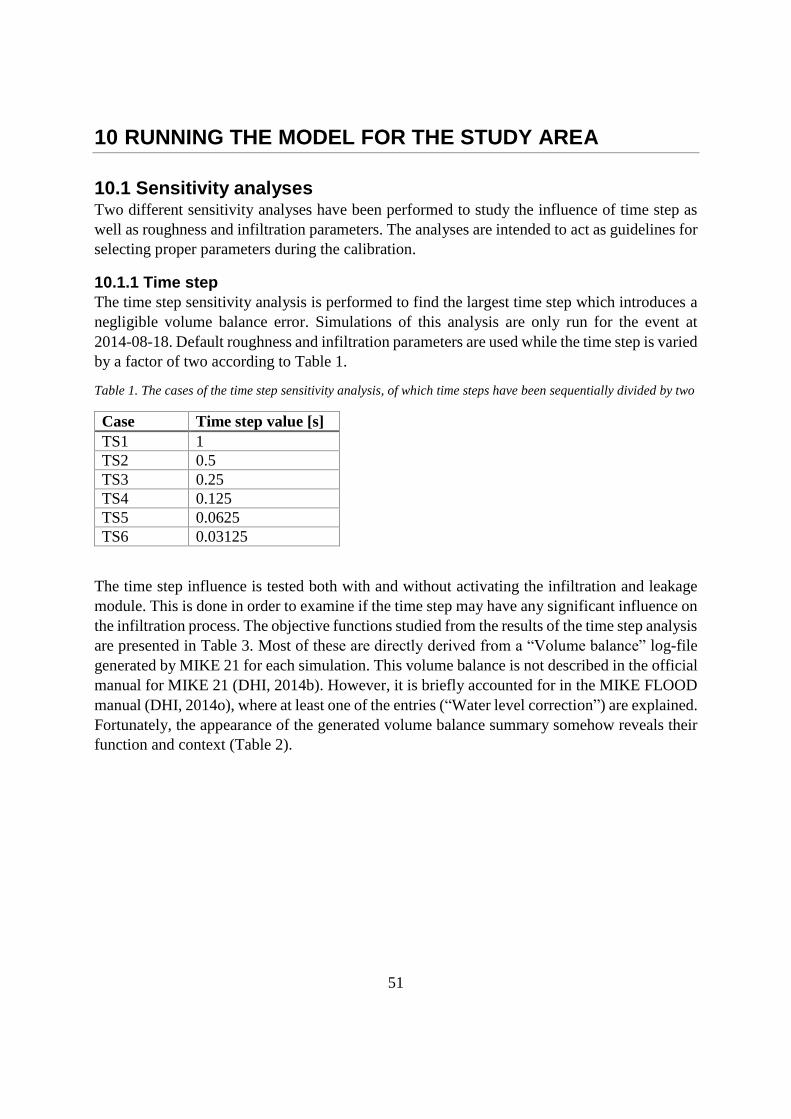
51
10 RUNNING THE MODEL FOR THE STUDY AREA
10.1 Sensitivity analyses Two different sensitivity analyses have been performed to study the influence of time step as
well as roughness and infiltration parameters. The analyses are intended to act as guidelines for
selecting proper parameters during the calibration.
10.1.1 Time step
The time step sensitivity analysis is performed to find the largest time step which introduces a
negligible volume balance error. Simulations of this analysis are only run for the event at
2014-08-18. Default roughness and infiltration parameters are used while the time step is varied
by a factor of two according to Table 1.
Table 1. The cases of the time step sensitivity analysis, of which time steps have been sequentially divided by two
Case Time step value [s]
TS1 1
TS2 0.5
TS3 0.25
TS4 0.125
TS5 0.0625
TS6 0.03125
The time step influence is tested both with and without activating the infiltration and leakage
module. This is done in order to examine if the time step may have any significant influence on
the infiltration process. The objective functions studied from the results of the time step analysis
are presented in Table 3. Most of these are directly derived from a “Volume balance” log-file
generated by MIKE 21 for each simulation. This volume balance is not described in the official
manual for MIKE 21 (DHI, 2014b). However, it is briefly accounted for in the MIKE FLOOD
manual (DHI, 2014o), where at least one of the entries (“Water level correction”) are explained.
Fortunately, the appearance of the generated volume balance summary somehow reveals their
function and context (Table 2).

52
Table 2. An example of a MIKE 21 log-file “Volume Balance Summary”, showing the key quantities needed for
analyzing model performance for different time steps
Engineers Australia (2012) present a similar mass balance (Equation 7), corresponding to the
MIKE 21 volume balance in Table 2. This can be shown by rearranging the equivalents of
both balance equations.
Equation 7. Volume balance (adopted
from Engineers Australia, 2012) 𝑉𝑜 = 𝑉𝑖 + 𝑉𝐵 + 𝑉𝑅 − 𝑉𝐿 − 𝑉𝑆 + 𝐸
where Equivalent in MIKE 21 volume balance (Table 2)
Vo = Outflow volume D
Vi = Initial volume in the
model
A
VB = Volume from external
boundaries
C = VB + VR – VL
VR = Volume of rainfall
VL = Volume of losses
VS = Volume in storages B
E = Volume error E

53
The “Relative deficit”, in the MIKE 21 volume balance summary, relates the error
(E: Continuity balance) to the maximum value of all main quantities (A, B, C, D). Similarly,
Engineers Australia (2012) relates the error (E) to the outflow volume (Vo) and further suggests
that acceptable values of E/Vo should be in the range 0% to 5%. If exceeded, numerical issues
should be considered.
Despite the limited guidance for interpreting the MIKE 21 volume balance summary, the
terminology and structure, as seen in Table 2, correlates well with the corresponding concept
of Engineers Australia (2012). This allows for an intuitive way to use the results for further
analysis. While the goal to keep “Water level correction” and “Continuity balance” close to
zero is of permanent interest, examination of the “Hydrology processes” becomes far more
interesting when infiltration is activated. The reasons are understood from the explanations and
interpretations of the objective functions, as seen in Table 3.
Table 3. The objective functions studied in the time step sensitivity analysis, some of them also seen in Table 2
Objective
function
Unit Interpretation and/or explanation
Hydrology
processes
m3 The total addition (or subtraction) of water from hydrological
processes such as precipitation, evaporation and infiltration
Water level
correction
m3 A volume correction adding to the total inflow – a large time
step may cause the water level in a cell to drop below the bed
level, and thus the water level needs to be adjusted to just
above zero (DHI, 2015b)
Total outflow m3 Total outflow from the model, i.e. all water leaving the model
during the simulation
Continuity
balance
m3 A simple mass balance, adding up all inflow/outflow and
initial/final model area volumes, to be kept close to zero
Qmax m3/s The maximum value from the extracted discharge series
Umax m/s The maximum velocity observed in any grid cell throughout
the simulation – required to calculate the Courant number
Courant number - As explained in section 9.1.2
Nash-Sutcliffe
coefficient
- The Nash-Sutcliffe index relating the discharge series for a
certain time step with the discharge series for the smallest time
step (0.03125 s)
Simulation time min The elapsed time for the simulation, analyzed only to identify a
reasonable time step to be used in order to fit all simulations
within the timescale of this study
To reach the goal of the time step sensitivity analysis, the results were analyzed in a way to find
out for which time step all the objective functions, except Courant number and simulation time,
converges. In other words, the advance towards smaller time steps is assumed to introduce
progressively less errors to the volume balance.

54
Likewise, by assuming that a smaller time step in general improves the stability and accuracy
of the model, Nash-Sutcliffe coefficients can be calculated for every time step by relating each
corresponding discharge series consistently to the series corresponding to the least of time steps
investigated (0.3125 s). Thus, in terms of Nash-Sutcliffe parameters, the least-time-step series
is analogous to the observed values and all others are analogous to modeled values.
10.1.2 Roughness and infiltration parameters
A sensitivity analysis was performed to study the influence of different model parameters. This
was done for the real rainfall event as well as the design rainfall. In total 16 different cases of
parameter value alternations, in addition to the default case, have been simulated.
The layer depth and porosity parameters have an almost equivalent function, i.e. controlling the
total bulk and pore volume per unit area of the infiltration layer. In fact, it would be possible to
control either one of them by adjusting the other. Therefore, the layer depth was chosen to
remain constant in all cases. The selection of model parameters included in the sensitivity
analysis is presented in Table 4 along with value alternations and corresponding default value.
In order to limit the sensitivity analysis further, also the leakage rate was kept constant. The
choice was made upon the assumption that the leakage rate should approximately correspond
to a rather low and spatially equally distributed saturated hydraulic conductivity in deep parts
of the soil.
Table 4. Parameter configurations used in the sensitivity analysis, showing each case with its corresponding
parameter alternation in comparison with the corresponding default case value.
Case Parameter Value Default
RA1 Manning's M - Asphalt [m1/3/s] 25 50
RA2 100
RG1 Manning's M - Gravel [m1/3/s] 15 30
RG2 60
RN1 Manning's M - Natural terrain [m1/3/s] 1 2
RN2 4
IRG1 Infiltration rate - Gravel [mm/h] 60 90
IRG2 120
IRN1 Infiltration rate - Natural [mm/h] 5 10
IRN2 20
IPG1 Porosity - Gravel [-] 0.15 0.3
IPG2 0.6
IPN1 Porosity - Natural terrain [-] 0.05 0.1
IPN2 0.2
IV1 Initial volume [%] 5 50
IV2 95

55
Most of the parameters were alternated by dividing and multiplying the default values (chosen
in chapter 9) by two. One exception is the case of infiltration rate for gravel, where the lower
and upper values were already available from the literature. Hence, the default value was set to
the mean value of these two. Moreover, it has already been indicated that the initial volume
parameter does not pose as a value to be ultimately determined during the calibration. Rather,
it used to set preconditions of the unsaturated zone for a certain simulation event. The most
natural choice of default value was therefore an initial water content of 50%, whereas the lower
and upper values were chosen to represent extreme scenarios (±5%) with initial water contents
of 5% and 95%, respectively.
Finally, the results have been compared to the results of the default case simulation in terms of
some objective functions - total accumulated flow, maximum peak flow and for the real event
also a peak ratio. During the rainfall event at 2014-08-18, two significant flow peaks can be
noted. The ratio of the first peak to the second is studied in order to control the interaction
between soil infiltration and saturation.
Table 5. The objective functions studied in the roughness and infiltration sensitivity analysis
Objective function Unit Explanation
Total accumulated flow m3 Accumulated volume from the extracted discharge series
Maximum peak flow m3/s Maximum value observed from the extracted discharge series
Peak 1:2 ratio % A ratio of two significant flow peaks – only for the real
rainfall event at 2014-08-18
10.2 Calibration and validation The calibration was performed for the event at 2014-08-18, by iteratively changing roughness
and infiltration parameters to get a proper match between simulated discharge data and the
refined observed flow meter data.
At the initiation of the calibration process, results from the default case simulation of the
sensitivity analysis are visually compared against flow meter data. Quantification of default
case deviation from other cases, in terms of the objective functions in Table 5 indicates which
parameters to be changed in order to equalize the appearance of simulated and measured
discharge data. To confirm the match, the Nash-Sutcliffe index is applied on the results.
Uncertainties regarding the rainfall and discharge data synchronization, significantly
complicates the calibration process. For example, if a time lag is observed between the modeled
and measured discharge, it is hard or even impossible to determine if the dissimilarity should
be fixed by calibration of certain roughness and infiltration parameters. Thus, manual time
shifting may be applied for the simulation results, in order to perfect the match. The legitimacy
of the time shift is not necessarily possible to confirm from the validation process, assuming
that the asynchronicity is not static throughout the analyzed time series.
The validation period ranges from directly after the calibration event and six days ahead, ending
at 2014-08-24. Normally, the calibration period should not be included in the validation period

56
(Hingray et al., 2015). Despite this, the validation simulation has the same starting point as the
calibration, for the purpose of including a groundwater model warm-up period for the
subsequent validation period. In other words, this sets the volume stored in the infiltration layer
before the validation, without having to make a qualified guess manually. In that sense, this
should not be considered a true validation, according to Hingray et al. (2015).
Most distributed models are evaluated in terms of catchment outlet discharge prediction, despite
the great possibilities for evaluating also against other variables, e.g. water levels, soil moisture
content and flows at different points within the model area (Beven, 2001). The model of this
study is also restricted to discharge evaluation at one point – the flow meter in the swale. In this
case the swale flow measurements were the only hydrological data available for calibration and
validation of the model. Thus, the choice of objective functions was not difficult. However, the
flow peaks and accumulated discharge have a certain importance for this type of SUDS. Since
the system is eventually drained by a stormwater pipe network, it was of interest to identify
under which conditions the pipe system has enough capacity to divert all the excess runoff it
receives.
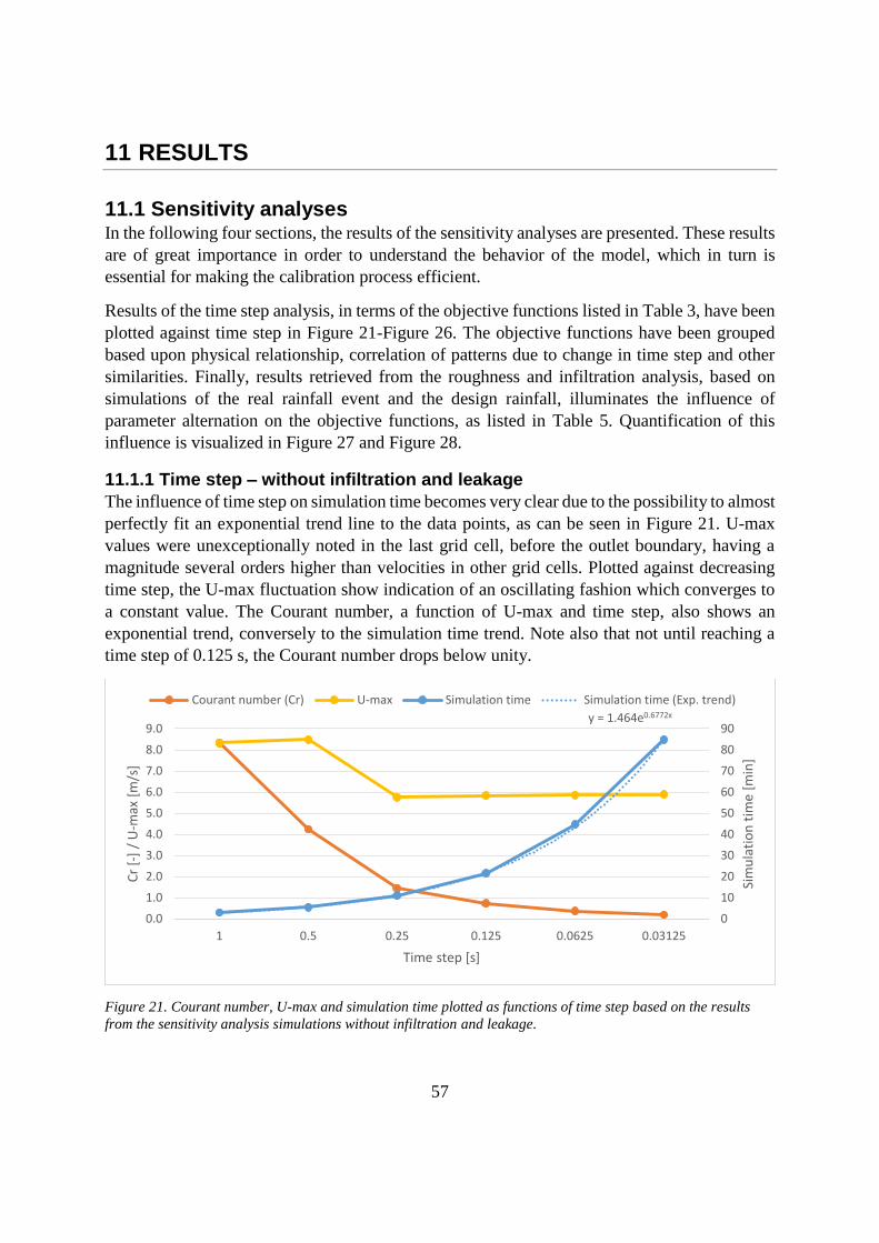
57
11 RESULTS
11.1 Sensitivity analyses In the following four sections, the results of the sensitivity analyses are presented. These results
are of great importance in order to understand the behavior of the model, which in turn is
essential for making the calibration process efficient.
Results of the time step analysis, in terms of the objective functions listed in Table 3, have been
plotted against time step in Figure 21-Figure 26. The objective functions have been grouped
based upon physical relationship, correlation of patterns due to change in time step and other
similarities. Finally, results retrieved from the roughness and infiltration analysis, based on
simulations of the real rainfall event and the design rainfall, illuminates the influence of
parameter alternation on the objective functions, as listed in Table 5. Quantification of this
influence is visualized in Figure 27 and Figure 28.
11.1.1 Time step – without infiltration and leakage
The influence of time step on simulation time becomes very clear due to the possibility to almost
perfectly fit an exponential trend line to the data points, as can be seen in Figure 21. U-max
values were unexceptionally noted in the last grid cell, before the outlet boundary, having a
magnitude several orders higher than velocities in other grid cells. Plotted against decreasing
time step, the U-max fluctuation show indication of an oscillating fashion which converges to
a constant value. The Courant number, a function of U-max and time step, also shows an
exponential trend, conversely to the simulation time trend. Note also that not until reaching a
time step of 0.125 s, the Courant number drops below unity.
Figure 21. Courant number, U-max and simulation time plotted as functions of time step based on the results
from the sensitivity analysis simulations without infiltration and leakage.
y = 1.464e0.6772x
0
10
20
30
40
50
60
70
80
90
0.0
1.0
2.0
3.0
4.0
5.0
6.0
7.0
8.0
9.0
1 0.5 0.25 0.125 0.0625 0.03125
Sim
ula
tio
n t
ime
[min
]
Cr
[-]
/ U
-max
[m
/s]
Time step [s]
Courant number (Cr) U-max Simulation time Simulation time (Exp. trend)

58
Water level correction (WLC) and continuity balance (CB) are both interpreted as indicators of
the model stability and should optimally be close to zero. From the results of the time step
analysis without infiltration, it can be noted that the CB is constant at -0.01 m3 for all time steps
(Figure 22). The WLC, however, introduces a large volume error of roughly 14 m3 when using
a time step of 1 s, but remains constant at 0 m3 for all other time steps.
The Nash-Sutcliffe (NS) correlation, i.e. the similarity of discharge series to the discharge series
of time step 0.03125 s, can in Figure 22 be seen converging to a perfect match when the time
step decreases. Already at the time step of 0.25 s, the NS converges to a value of 1 and a perfect
match.
Figure 22. Water level correction, continuity balance and Nash-Sutcliffe coefficient plotted as functions of time
step based on the results from the sensitivity analysis simulations without infiltration and leakage.
Similar to the WLC, the hydrological objective functions outflow volume (OV) and Q-max
settles to constant values (160.78 m3 and 0.028 m3/s respectively) for time steps of 0.5 s and
below (Figure 23). Hydrology processes (HP) remains constant for all time steps (169.04 m3).
For the time step of 1 s, the OV and Q-max are slightly higher than for the smaller time steps.
Note that this OV deviation corresponds to the same volume as the WLC for the same time step
(see Figure 22).
Since the volume errors in the CB’s are negative, also the relative errors become negative. Thus,
if the acceptance range of Engineers Australia (2012) ignores the sign of the relative error, it
will fulfill the recommended criteria.
0.90
0.92
0.94
0.96
0.98
1.00
1.02
-2
0
2
4
6
8
10
12
14
16
1 0.5 0.25 0.125 0.0625 0.03125
NS
coef
fici
ent
[-]
WLC
/ C
B [
m³]
Time step [s]
Water level correction (WLC) Continuity balance (CB) Nash-Sutcliffe (NS)

59
Figure 23. Outflow volume, hydrology processes and Q-max plotted as functions of time step based on the
results from the sensitivity analysis simulations without infiltration and leakage.
11.1.2 Time step – with infiltration and leakage
When infiltration and leakage is activated, the results of the time step sensitivity analysis show
rather different patterns although some similarities can be noted.
The simulation time still shows an exponentially growing trend (Figure 24), just like the case
without infiltration and leakage. In contrast to this resemblance, the U-max indicates a
continuously growing trend which does not seem to converge. Nevertheless, the Courant
number decreases in an exponential-like manner similar to the analysis without infiltration and
leakage. For the largest time step, the Courant number barely exceeds one, but falls far below
unity for smaller time steps.
Figure 24. Courant number, U-max and simulation time plotted as functions of time step based on the results
from the sensitivity analysis simulations with infiltration and leakage.
0.000
0.005
0.010
0.015
0.020
0.025
0.030
0.035
150
155
160
165
170
175
180
1 0.5 0.25 0.125 0.0625 0.03125
Q-m
ax [
m³/
s]
OV
/ H
P [
m³]
Time step [s]
Outflow volume (OV) Hydrology processes (HP) Q-max
y = 1.8355e0.6589x
0
20
40
60
80
100
120
0.0
0.2
0.4
0.6
0.8
1.0
1.2
1.4
1.6
1.8
1 0.5 0.25 0.125 0.0625 0.03125
Sim
ula
tio
n t
ime
[min
]
Cr
[-]
/ U
-max
[m
/s]
Time step [s]
Courant number (Cr) U-max Simulation time Simulation time (Exp. trend)

60
A WLC for time step 1 s can be noted but is relatively small (0.71 m3). For smaller time steps
the WLC is zero. With infiltration and leakage activated, the CB is no longer independent of
time step. Instead, it decreases with decreasing time step, with tendency to converge (Figure
25). However, the drop at the smallest time step suggests a continuously decreasing trend.
The NS correlation shows a noticeable deviation from the target for time step 1 s and in this
case also for the time step 0.5 s. A perfect match is never reached, however, from 0.125 s and
below the correlation is very close to perfect (>0.999).
Figure 25. Water level correction, continuity balance and Nash-Sutcliffe coefficient plotted as functions of time
step based on the results from the sensitivity analysis simulations with infiltration and leakage.
The objective functions of OV, HP and Q-max all show growing trends as the time step
decreases (Figure 26). It should be noted though, that the trends seem to converge from time
step 0.125 s and smaller. Yet, comparable but conversely to the CB, these trends steps up
additionally at the smallest time step, thus breaking the convergence.
All relative errors are within the acceptable range, according to Engineers Australia (2012).
0.93
0.94
0.95
0.96
0.97
0.98
0.99
1.00
0
0.1
0.2
0.3
0.4
0.5
0.6
0.7
0.8
1 0.5 0.25 0.125 0.0625 0.03125
NS
coef
fici
ent
[-]
WLC
/ C
B [
m³]
Time step [s]
Water level correction (WLC) Continuity balance (CB) Nash-Sutcliffe (NS)

61
Figure 26. Outflow volume, hydrology processes and Q-max plotted as functions of time step based on the
results from the sensitivity analysis simulations with infiltration and leakage.
11.1.3 Roughness and infiltration – real rainfall event
In this section, the impact of roughness and infiltration parameters on discharge generated by
the real rainfall event, is presented by commenting differences between objective functions of
the default case and all other test cases. The results are quantified and visualized in Figure 27.
Alternation of natural terrain roughness has, in relation to the other surface types, substantial
impact on all three objective functions. Furthermore, all the objective functions decreases with
decreased parameter value and vice versa. Nevertheless, a reduced asphalt roughness also
indicates comparatively significant influence. However, while the accumulated outflow and
peak flow is reduced, the peak 1:2 ratio increases.
The infiltration parameters, infiltration rate and porosity, have the greatest impact in zones
composed of gravel. In that case, a reduced infiltration rate increases all objective function
whereas an intensified rate does the opposite. On the other hand, a reduced gravel porosity
greatly increases accumulated outflow and peak flow but decreases the peak 1:2 ratio.
Naturally, a greater gravel porosity results resembles the opposite. Noteworthy is also that the
infiltration rate of natural terrain also has significant impact on the peak 1:2 ratio, even more
than the gravel infiltration rate.
Near-saturated conditions of the infiltration layer, represented by setting the initial volume to
95%, had in this case enormous influence on accumulated flow and peak flow. However, the
peak 1:2 remained nearly unchanged (only +2% deviation). An almost dry infiltration layer,
corresponding to 5% initial volume, also had significant impact; however, in this case on all
objective functions and rather of the same magnitude as the other infiltration parameters with a
notable impact. Moreover, these effects were very similar to the product of increased gravel
porosity.
0.007
0.008
0.009
0.010
0
10
20
30
40
50
60
1 0.5 0.25 0.125 0.0625 0.03125
Q-m
ax [
m³/
s]
OV
/ H
P [
m³]
Time step [s]
Outflow volume (OV) Hydrology processes (HP) Q-max

62
Figure 27. Percental deviation from the default case of the 2014-08-18 simulation, in terms of the objective
functions accumulated outflow, peak flow and peak 1:2 ratio. As a reminder, the naming of the cases (presented
in Table 4) should be read by starting with the parameter type (R – roughness, IR – infiltration rate, IP –
infiltration porosity, IV – infiltration initial volume) followed by surface/layer type (A – asphalt, G – gravel, N –
natural terrain) and a change of the parameter value (1 – decrease, 2 – increase).
11.1.4 Roughness and infiltration – design rainfall event
The roughness and infiltration parameters have in general less impact on the accumulated
outflow and peak flow when simulating for the 10-year design storm, compared to the real
rainfall event. This can be seen from the results in Figure 28. However, there are some striking
exceptions. For example, the increase in roughness of natural terrain increases the peak flow
with 79%, compared to +12% for the same parameter change when simulating for the real
rainfall event.
Increasing the initial volume to 95% does not cause any major change in peak flow. However,
this parameter alternation significantly increases the accumulated flow (+72%), although only
half as much as for the case of the real rainfall event. Aside from the great increase in peak flow
due to increased natural terrain roughness, the accumulated flow is the most affected objective
function for the design rainfall simulation.
-25% 0% 25% 50% 75% 100% 125% 150% 175% 200%
RA1
RA2
RG1
RG2
RN1
RN2
IRG1
IRG2
IRN1
IRN2
IPG1
IPG2
IPN1
IPN2
IV1
IV2
Deviation from default case - 2014-08-18
Accumulated outflow Peak flow Peak 1 / Peak 2

63
Figure 28. Percental deviation from the default case of the design rainfall simulation, in terms of the objective
functions accumulated outflow and peak flow. As a reminder, the naming of the cases (presented in Table 4)
should be read by starting with the parameter type (R – roughness, IR – infiltration rate, IP – infiltration
porosity, IV – infiltration initial volume) followed by surface/layer type (A – asphalt, G – gravel, N – natural
terrain) and a change of the parameter value (1 – decrease, 2 – increase).
11.2 Calibration After several iterations during the calibration process, the parameter configuration seen in Table
6 was found to best match observed and modeled discharge. Furthermore, the entire model data
series had to be time-shifted 8 minutes ahead, in order to achieve a proper timing (see Figure
29). Notably, the natural terrain roughness had strong influence on the timing of flow peaks.
Table 6. Final parameter values after calibration
Surface/soil type Roughness [m1/3/s] Infiltration rate [mm/h] Porosity [-]
Asphalt 50 0 0
Gravel 30 80 0.13
Natural terrain 1.75 50 0.08
-25% 0% 25% 50% 75% 100% 125% 150% 175% 200%
RA1
RA2
RG1
RG2
RN1
RN2
IRG1
IRG2
IRN1
IRN2
IPG1
IPG2
IPN1
IPN2
IV1
IV2
Deviation from default case - CDS of 10 years recurrence
Accumulated outflow Peak flow

64
Figure 29. Measured discharge compared with modeled discharge after calibration and time-shifting of 8 min
forward. The non-shifted model series is also plotted to visualize the timing issue.
By using the parameter values in Table 6, a Nash-Sutcliffe coefficient of 0.863 was calculated
to represent the correlation between observed and modeled data during the calibration period.
Small deviations in accumulated flow and flow peaks, between observed and modeled data,
were observed and are presented in Table 7.
Table 7. Summary of final-calibration-simulation results in terms of the objective functions, comparing modeled
discharge (M21) and observed flow data (ISCO).
Objective function M21 ISCO Deviation – (M21-ISCO)/ISCO
Peak 1 [m3/s] 0.00435 0.00463 -6%
Peak 2 [m3/s] 0.00880 0.00885 -1%
Peak 1:2 ratio 49% 52% -6%
Accumulated discharge [m3] 41.98 42.56 -1%
11.3 Validation Since the entire validation period is comparatively long, the results are split into three smaller
parts (as seen in Figure 30-Figure 32) for further analysis. All these parts include recognizable
discharge events, both modeled and observed, along with associated rainfall event data.
However, starting from late 2014-08-21/early 2014-08-22 and ending in late 2014-08-23, there
is a period of insignificant records in all series. This “gap” is not further analyzed but noted to
indicate validity of the model during this period.
0.000
0.002
0.004
0.006
0.008
0.010
14:00 17:00 20:00
Dis
char
ge [
m³/
s]
Processed ISCO flow data Time-shifted MIKE 21 Simulation MIKE 21 Simulation

65
The first part of the validation period, stretching from 2014-08-19 to 2014-08-22, contains
observable rainfall events and modeled flow peaks on each of the three days (Figure 30).
However, according to the observed flow data, the flow meter did not record any discharge
whatsoever during the first day. The model, for that matter, responded distinctively to the short
but rather intense rainfall inputs of the same period. On the following day, both the model and
flow meter responded to the corresponding rainfall, having a more pronounced duration.
Although there are evident timing dissimilarities, some peaks correlate rather well and so does
the total volume. During the third day, the most noticeable outcome is the slight overestimation
of both peaks and volume. The Nash-Sutcliffe coefficient for this part indicated very poor
correlation with a value of -0.635. Furthermore, the model produced 78% more accumulated
discharge for the same period.
Figure 30. Validation results – part 1: 2014-08-19 – 2014-08-22. Notable is the modeled flow peak on the first
day, caused by intense rainfall with rather short duration. A corresponding response was not recorded by the flow
meter at all.
Part two of the validation period showed the best correlation although the Nash-Sutcliffe
coefficient was still very low (-0.267). However, the accumulated discharge from the model
only exceeded the observed with 2%. From Figure 31 it can be seen that the modeled peaks are
in general a bit early and too high, sometimes doubled. Another phenomenon to take notice of,
also occurring in part one but more evidently in this part, is the quick fall of the modeled
discharge rate directly after a rainfall event. Parallel to this, the observed discharge rate declines
much slower and occasionally levels out in a baseflow-like fashion.
0
5
10
15
20
25
30
35
40
45
500.000
0.001
0.002
0.003
0.004
0.005
0.006
2014-08-19 2014-08-20 2014-08-21 2014-08-22
Rai
nfa
ll in
ten
sity
[m
m/h
]
Dis
char
ge [
m³/
s]
Processed ISCO flow data MIKE 21 Simulation Rain intensity

66
Figure 31. Validation results – part 2: 2014-08-23 – 2014-08-24. Note the slowly decreasing baseflow-like pattern
of the observed discharge directly after a rainfall event – an appearance of almost complete absence in the
corresponding modeled discharge.
The last and third part of the validation period (2014-08-24 – 2014-08-25) demonstrates the
greatest exception in magnitude of flow peaks as well as accumulated discharge. Despite this,
the overall timing of the peaks correlates rather well, however, as previously noted, starts a bit
early. As a consequence of the two rather extreme flow peaks, the modeled accumulated
discharge becomes 114% larger than the observed value. A Nash-Sutcliffe coefficient of -15.93
indicates an extremely poor correlation.
Figure 32. Validation results – part 3: 2014-08-24 – 2014-08-25. Note that the range of both axes differs from
Figure 30 and Figure 31. The modeled flow peaks and rainfall intensities for this period are significantly higher
than for the two others.
0
5
10
15
20
25
30
35
40
45
500.000
0.001
0.002
0.003
0.004
0.005
0.006
2014-08-23 21:00 2014-08-24 09:00 2014-08-24 21:00
Rai
nfa
ll in
ten
sity
[m
m/h
]
Dis
char
ge [
m³/
s]
Processed ISCO flow data MIKE 21 Simulation Rain intensity
0
10
20
30
40
50
60
70
80
90
1000.00
0.01
0.02
0.03
0.04
0.05
2014-08-24 21:00 2014-08-24 22:00 2014-08-24 23:00 2014-08-25 00:00
Rai
nfa
ll in
ten
sity
[m
m/h
]
Dis
char
ge [
m³/
s]
Processed ISCO flow data MIKE 21 Simulation Rain intensity

67
Finally, the entire period (2014-08-19 – 2014-08-25) was validated – for this period, the
modeled accumulated discharge exceeded the observed accumulated discharge by 58% and the
Nash-Sutcliffe coefficient was -3.45.
11.4 Comparison with the MIKE SHE model The MIKE SHE model was a preliminary version, meaning that calibration had not been fully
completed before it was run in order to produce the results evaluated against the results of the
MIKE 21 model. Both models share the same inputs in terms of rainfall data and DEM,
including catchment area, but are in other aspects built independently. As a result of using the
same rainfall data series, and based on the previously discussed timing issues, the MIKE SHE
model discharge series was also time-shifted 8 minutes ahead. Additionally, The MIKE SHE
results were only available for the period 2014-08-18 – 2014-08-22. Due to these shortcomings,
the results were analyzed both qualitatively and quantitatively, with focus on the qualitative
performance, e.g. similarities in trends seen from the response of discharge to rainfall. Here
follows a comparison of the observed and modeled discharge series split into two parts.
The first part, corresponding to the calibration period, includes visually similar trends in the
results from the two models and observed data, as seen in Figure 33. Initially, the MIKE SHE
model tends to estimate the discharge response similarly to, and in the same order of magnitude,
as observed and MIKE 21 discharge. The first flow peak differs from the observed peak by
-18% (the corresponding deviation for MIKE 21 is -6%). Thereafter, the discharge is
continuously underestimated. The total accumulated discharge is -64% lower than the observed.
In addition, the second peak is of about the same magnitude as the first one, in fact 2% lower.
This contrasts to the observed data where the first peak only makes up 52% of the second peak.
Figure 33. Modeled discharge from the MIKE 21 and MIKE SHE calibration-period simulation, together with
observed discharge and rainfall intensity for the same period. The model discharge is time-shifted 8 minutes ahead.
0
10
20
30
40
50
60
70
80
90
1000.000
0.002
0.004
0.006
0.008
0.010
0.012
0.014
2014-08-18 13:00 2014-08-18 16:00 2014-08-18 19:00
Rai
nfa
ll in
ten
sity
[m
m/h
]
Dis
char
ge [
m³/
s]
Processed ISCO flow data Time-shifted MIKE 21 Simulation
Time-shifted MIKE SHE Simulation Time-shifted rain intensity

68
In part two, covering the period from 2014-08-19 to 2014-08-22, the discharge underestimation
continues (Figure 34). However, during 2014-08-19, the MIKE SHE result indicates response
to the two intense rainfall events, as indicated also by the MIKE 21 model but not in the
observed data. The deficit in accumulated discharge volume, for MIKE SHE results compared
to observed data, was -11% for the entire simulation period, i.e. both parts together. For the
same period, the MIKE 21 model produced 25% more accumulated discharge than the observed
data.
Figure 34. Modeled discharge from the MIKE 21 and MIKE SHE post-calibration-period simulation, together
with observed discharge and rainfall intensity for the same period. MIKE SHE data were not available for the
period after 2014-08-22. The model discharge is time-shifted 8 minutes ahead.
No indications of baseflow-like discharge behavior (as seen in the observed discharge data)
could be noted in the MIKE SHE simulation results. The overall discharge behavior of the
MIKE SHE model discharge is quite similar to the MIKE 21 model discharge but clearly with
rates and volumes of several orders of magnitude lower.
0
10
20
30
40
50
60
70
80
90
1000.000
0.001
0.001
0.002
0.002
0.003
0.003
2014-08-19 2014-08-20 2014-08-21 2014-08-22
Rai
nfa
ll in
ten
sity
[m
m/h
]
Dis
char
ge [
m³/
s]
Processed ISCO flow data MIKE SHE Simulation MIKE 21 Simulation Rain intensity

69
12 DISCUSSION
12.1 A lack of knowledge? The literature search of this study was unable to submit adequate pre-existing information about
true two-dimensional hydrodynamic modeling, i.e. using no links to other modeling systems,
for the purpose of describing hydrological processes in subcomponents of separate SUDS
devices. Nor could any non-DHI literature, describing constant-infiltration-rate 2D loss models,
be found. This does not mean that there is no such literature. Possibly, even more relevant
literature could have been found if the search was not limited to MIKE 21 specifically. Other
2D modeling software (e.g. Rojas et al., 2007) are known to share at least some of the central
features with MIKE 21 and its infiltration and leakage module. There are also strong indications
that 2D loss models is a recognized concept (e.g. Engineers Australia, 2012). Most likely, the
fact that the infiltration and leakage module of MIKE 21 is not yet officially released, also
influences the suggested lack of knowledge. The question remains if the infiltration and leakage
module of MIKE 21 is unique in applying a constant infiltration rate. This is further discussed
in the following section.
12.2 Modeling hydrological losses in MIKE 21 In order to evaluate the authenticity of the MIKE 21 model, we consider the author’s perceptual
model as the closest we can get to the hydrological processes in reality. The greatest difference
between these two models is the process of groundwater flow. In a way, the MIKE 21
infiltration can be seen as a pseudo-vertical-flow, since water enters the soil from above by
infiltration and leaves the same storage by leaking out below. However, the MIKE 21 model’s
representation of horizontal groundwater flow is completely absent. In contrast, the perceptual
model describes a groundwater flow, from low to high hydraulic potential, which might as well
be vertical and horizontal in combination. For example, some of the infiltrated water could, as
result of saturation, eventually become surface runoff after partially vertical transport through
the soil, as reviewed by Beven (2001). This model restriction could possibly be a part of the
reason why the modeled discharge rate declines very fast after a rainfall event, contrary to the
base-flow like pattern seen in the observed discharge data (e.g. Figure 31). Other potential
reasons are discussed later in this chapter.
By holding a much simplified formulation of the infiltration process, the infiltration and leakage
module of MIKE 21 stands out among the approaches of other hydrological models featuring
infiltration functionality. When using a constant infiltration rate, it should however not be more
difficult to approximate the actual total volume loss from infiltration than when using a
physically more correct method, such as for example Horton or Green-Ampt. Consider the
example in Figure 35, where the same total volume loss from infiltration is achieved by using
a constant infiltration rate and an exponential infiltration rate, according to the Horton method.
If both methods have equal initial and final infiltration rate, the state of saturation has to be
reached much earlier when using a constant infiltration rate, in order to infiltrate the same total
volume.

70
Figure 35. Comparison of constant and Horton infiltration rate, with the same initial and final rate. The area
under each graph, corresponding to the total volume loss from infiltration, are equal.
The difference in infiltration pattern, as seen in Figure 35, will most likely also affect the pattern
or shape of the discharge curve, especially when modeling rather small systems at fine temporal
scale. Thus, although a constant infiltration rate probably would capture the overall effects of
an infiltration process, in terms of total volume loss at a seasonal basis, it will be necessary to
reflect on whether it is a proper representation on finer scale.
As presented in section 5.2.1, there are even more simplified methods for making a rough
subtraction of infiltrated volume from inflow volume, thus indirectly also from the outflow
volume. Some questions then arise: could such methods be equally appropriate to a constant-
rate infiltration formulation under certain circumstances? Is the constant-rate formulation in
fact an intermediate of these methods and the physically-based formulations of for example
Horton and Green-Ampt?
The first question may be answered with disagreement for situations where the surfaces and
soils of the model area are all heterogeneous and spatial distribution of infiltration properties is
of great importance. In addition, delay effects of “early” flow peaks, following unsaturated soil
conditions, may be hard to simulate using only the input-reducing methods.
The answer to the second question is less straightforward and rather leads to another question:
why does the infiltration and leakage module of MIKE 21 make use of a constant infiltration
rate formulation instead of the just about as simple, but more physically correct formulations
of for example Horton and Green-Ampt? The Horton approach, in its original form, would
require at maximum two more input parameters, however, the dependence of time could make
the implementation impractical, thus suggesting alternative formulations (e.g. Gabellani et al.,
2008). Likewise, the Green-Ampt equation requires four parameters for model implementation
(Rojas et al., 2007), of which two are already required by the infiltration and leakage module
in MIKE 21. Furthermore, physically-based infiltration parameter values (found in for example
Rawls et al., 1983, Svenska vatten- och avloppsverksföreningen, 1983) to be used for these
models should be easier to find than constant infiltration rates, as suggested by G. Barmen
(personal communication, March 10, 2015).
0
10
20
30
40
0 5 10 15 20Infi
ltra
tio
n r
ate
[mm
/h]
Time [min]
Horton Constant

71
A part of the answer, to the third and final question, may be found in the alternative approach
of using the infiltration and leakage module for direct rainfall applications, as described in the
manual of the same module (see section 8.2.2). The presentation of this methodology suggests
that this loss model is not primarily intended to model a physical representation of infiltration
processes in inland applications. Yet again, we are reminded of the original marine applications
of MIKE 21, where infiltration of for example rainfall on dry land may be less important.
The hydrological model of Solbacken is not alone in excluding evapotranspiration. In fact, this
simplification is rather common for rainfall-runoff models, although the process might be
important for a correct representation of seasonal variations (Hingray et al., 2015). However,
the simulations in this study have been delimited to range over a period of maximum 1-2 months
during late summer of one year. Therefore, the effects of evapotranspiration are possibly only
seen from a continuous and constant loss, which in the model may be compensated, and thus
represented, by leakage from the unsaturated zone. Beven (2001) also stresses the necessity of
estimating actual evapotranspiration losses for longer periods of rainfall-runoff simulations.
Nevertheless, a daily variation in evapotranspiration could be estimated by a simple sine curve
(Beven, 2001). This method could be implemented in MIKE 21 by specifying the evaporation
from a generated time series.
12.3 The issue of data reliability and accuracy It is extremely important to keep in mind that the reliability of collected data may be very
limited. Furthermore, the processing of data, especially of topography and precipitation, has
most likely introduced even more errors due to interpolation.
As a result of the difficulties to produce a reliable DEM, in combination with uncertainties
regarding the functionalities of the asphalt bumps, characteristics of the catchment area also
becomes a great source of uncertainty. For example, how accurate the information about the
extension of the eastern asphalt bump is, becomes crucial for determining how large the
upstream catchment area really is (see Figure 6). Imagine the area without this asphalt bump: a
great portion of the parking lot would then instead conduct surface runoff over the east slope
and into a part of the swale which does not connect to the flow meter. According to the author,
this was indeed a borderline case which could imply any of these possibilities in reality.
However, the actual truth could presumably never have been found. Nevertheless, a choice had
to be made.
Perhaps most evidently, the size of the catchment strongly influences the accumulated volume
from the outflow of the model. Simultaneously, a correct estimation of total volume relies no
less on proper hydrological input data and simulation of loss from the model, e.g. precipitation
and infiltration. Thus, it is hard to tell if a good match is achieved by the fact that errors, in
catchment size and rainfall data, cancel out each other. In addition, another possibility is that
ill-founded calibration of infiltration parameters may be able to produce good output from bad
input.

72
In order to calibrate and validate the model successfully, it is obvious that the input data, in
terms of rainfall, and calibration data, i.e. observed discharge, must be reliable and correct. As
there is no guarantee for this, whatsoever, this may be one of many reasons for the bad
correlation resulting from the validation. There are a couple of examples in Figure 30 and Figure
32 where the model responds distinctively to very intense, but often short rainfall events, which
were not recorded correspondingly by the flow meter. Consequently, these dissimilarities in
modeled and observed data introduces the largest deviations in accumulated volume but also
the general correlation, quantified by the Nash-Sutcliffe coefficient. A number of explanations
may be suggested as plausible:
Measurement errors at the rain gauge, e.g. spontaneous recording of non-existing
rainfall
General measurement errors by the flow meter
Some mechanism of inertia was not successfully implemented in the model, causing
very quick surface runoff which may infiltrate to a lesser degree (this is in fact also
indicated by the fast decline in discharge rate directly after most rainfall events)
The mechanism of the last bullet could be a result of an inadequate representation of the swale.
This idea is developed in the following section.
12.4 Swale and infiltration surface representation and the impact of
roughness and infiltration parameters A valuable outcome from the roughness and infiltration parameter sensitivity analysis, is the
significant impact of natural terrain roughness on peak flows. Although peak flows in general
were less affected by parameter changes for the design 10-year rainfall, the impact of natural
terrain roughness is indicated as important for both small and large events. The natural terrain
is mainly associated with surfaces close to and in the swale. This suggests that the representation
of the swale and its roughness properties are dominating the magnitude of the outflow rate,
irrespective of the type of rainfall. The finding is not entirely new; Engineers Australia (2012)
declares that Manning’s value is most influential on the model’s results along main flow paths,
such as creeks or open channels. Therefore, it is also relevant to question whether a 1 m grid
resolution is fine enough for describing the flow in this type of swale. Currently, it is more
beneficial of modeling one-directional flow in sub-grid scale features (e.g. swales) using a 1D
model. Using a 2D model, would require a significantly finer grid resolution for this application,
resulting in slow simulations (Engineers Australia, 2012). Thus, a combination of a 1D and 2D
domain could optimize the performance, as implemented in for example MIKE FLOOD (DHI,
2014o) or CASC4D (Rojas et al., 2007).
Potential difficulties of a proper model representation of the swale at Solbacken could also
explain the previously discussed fast declines in post-event discharge rate. There is an apparent
delay and signs of inertia for the measured swale flow, which also may suggest difficulties of
modeling surface resistance on flow. As another example, two quite extreme model flow peaks
during the late validation period, seen in Figure 32, could also indicate bad swale representation,

73
supposing the inability to model enough flow resistance under certain circumstances. As a
consequence, the discharge responds notably to intense rains. Whether this instead is a matter
of inaccurate rainfall data, unreliable flow meter data or even bad setup of the outlet boundary,
could preferably be examined.
Worth mentioning is also the pronounced effect of the gravel layer’s infiltration properties on
all objective functions monitored. Interestingly, these properties have significant impact on the
accumulated outflow for both rainfall events. This indicates that the design of this drainage
system may be relevant also for rainfalls of greater magnitude. Nevertheless, it must again be
stressed that the properties of this layer are very rough estimations, especially the layer depth.
Moreover, vertical (and horizontal) heterogeneity of the layer is assumed. In reality though, it
is not unlikely that the layer is stratified, thus possibly having dramatically less infiltration
capacity. The exact location of the same layer may however be of more importance.
As seen from the final parameter configuration after calibration (Table 6), the porosity values
for gravel and natural terrain are ultimately rather alike (0.13 and 0.08 respectively). At least
with respect to what in the literature is considered reasonable values for corresponding
measured (effective) porosity of these soil types, previously reflected on within section 7.3 and
9.2.2. There may be many reasons for why these quantities are ill-posed. Beven (2001), for
example, thoroughly outlines the difficulties of gathering values, from both measurements and
estimation, for coming up with an optimal parameter set which is valid also aside from during
calibration. Nevertheless, this study has already questioned the authenticity of the porosity
model parameter (see section 8.2), suggesting that it instead may be used to compensate for
improper layer depths, which also were very hard to determine. In addition, also the validity of
the layer depth concept of the model has been questioned. All this in combination makes it
impossible, at least very hard, and perhaps also irrelevant to validate these quantities.
12.5 Boundary conditions and time step selection Possibly one of the greatest limitations, when modeling small-scale inland flooding in MIKE
21, is the requirement of manually setting the model domain equal to the catchment area.
However, this does not necessarily has to be a prerequisite when modeling on large scale (cf.
Filipova, 2012, Mårtensson and Gustafsson, 2014). Moreover, modeling of the outlet is
something which needs to be handled in a much more sophisticated way. Consider once again
the SUDS modeling on larger scale – establishment of links to a pipe modeling system, or the
possibility for internal point sinks to operate on occasionally dry land, would then be necessary.
A striking fact from the time step sensitivity analysis is the great influence on the volume
balance when infiltration is activated. The mechanisms behind this phenomenon are not known
and can only be speculated on at this stage. The linearity of the one-dimensional continuity
equation, describing the infiltration process, should at first glance not be dependent on the
choice of time step. Perhaps a faster fluctuation in flooding and drying of cells could affect the
overall amount of water available for infiltration. Engineers Australia (2012) state that a
flooding and drying mechanism (see section 8.1), in combination with application of direct

74
rainfall (see section 5.2.1), may introduce pronounced volume errors when modeling shallow
overland flows on steep slopes. Such errors could in principle not be observed from the results
of the sensitivity analysis where the direct rainfall approach was used and infiltration
deactivated. However, it is not unlikely that these effects are somehow related. A proper
selection of time step is not completely obvious, based on the results of this analysis. Still, this
strongly suggests that the time step selection should be carried out even more carefully when
modeling infiltration in MIKE 21.
12.6 Assessing the validity of the MIKE 21 model As seen from the results, the MIKE 21 model was satisfactorily calibrated but could not be fully
validated. A clear pattern of the modeled discharge from the post-calibration period is seen
from the results – the modeled flow peaks starts in general a bit earlier and quite often reaches
a higher magnitude than the observed peaks (see for example the second validation part in
Figure 31). This suggests that some parts of the infiltration layer (or unsaturated zone), probably
near the swale, were too saturated prior to the rainfall event. Therefore, it is possible that a
better match between modeled and observed long-term discharge series could have been
achieved by increasing the leakage rate. As is known, the leakage rate parameter was excluded
from the sensitivity analysis and thus set to a constant value. With hindsight, it could in fact
have been beneficial to try to optimize this parameter during extended calibration with longer
simulation periods.
Unfortunately, results from a final and calibrated version of the MIKE SHE model was not
available. Consequently, the possibilities for evaluating the MIKE 21 model based on these
results were very limited. Apparent differences between the MIKE SHE discharge and observed
discharge data, certainly indicates the need of further calibration. Thus, a quantitative
comparison, in terms of discharge peaks and accumulated discharge, seems pointless. A
qualitative analysis indicated similarities between the models in terms of discharge behavior
(aside from magnitude and volume) as well as the absence of baseflow-like patterns. Currently,
this suggests that their level of describing the hydrological processes may as well be equivalent.
However, this would require further examination and significantly more data, with higher
reliability.
Nonetheless, there is some information of particular interest that can be used to strengthen
previous interpretations. For example, although the MIKE SHE discharge rates in general seem
to be greatly underestimated, the model discharge still responds, similarly to MIKE 21, to some
of the rainfall events for which the corresponding runoff is not indicated by the flow meter (see
for example Figure 34). This could either suggest a general difficulty in modeling the discharge
response to similar rainfall events or perhaps more likely, pronounced errors in the processed
rainfall or flow data. In general, the MIKE 21 model predicts magnitude of flow peaks rather
well compared to the MIKE SHE model. In contrast, the total accumulated discharge simulated
by MIKE SHE, deviates less from the observed volume. This indicates that both models have
difficulties with balancing flow peaks contra accumulated discharge. Still, as already discussed,
the reason might as well be due to data errors.

75
13 CONCLUSIONS
The goal of this study was to identify how and under which conditions the 2D hydrodynamic
and infiltration model of MIKE 21 is able to describe the stormwater system at Solbacken
satisfactorily. To be concluded from this study is that the model, under current preconditions,
was possible to calibrate but did not perform well during the validation. A plausible
explanation for these difficulties is a combination of poor input and calibration data, ill-
founded model assumptions as well as limitations of the basic model.
However, analysis of both the good and poor results showed that the swale representation,
notably in terms of assigned roughness values, is of great importance. Although swales are
commonly and most suitably represented by 1D models, it was of interest in this study to make
a complete 2D representation. Further studies are required in order to find optimal approaches
for 2D representation of swales included in models of the current type. Also concluded, was
that the model representation of gravel infiltration layers provided the intended effect on the
outflow, despite the difficulties of estimating layer properties.
Nevertheless, the principles of the infiltration model in MIKE 21 were questioned, in particular
the use of a constant infiltration rate. There are at least a couple of alternative infiltration
models, nearly as simple and easy to implement, possessing a more physically correct
description of the infiltration processes in reality. It is also suggested that the constant
infiltration rate formulation restricts the possibility to represent fine variations in the discharge
pattern. Additionally, there are indications of that the infiltration and leakage module is
currently not optimally designed, and possibly not even intended, to model infiltration in inland
applications. Finally, in order to avoid the risk of introducing large volume errors when using
this function, the time step of the model must be chosen with great care.
The performance of the MIKE 21 model could not be fully evaluated against the MIKE SHE
model, due to the absence of an ultimately calibrated version of the latter. However, the MIKE
SHE simulation results provided valuable information about potential data errors or
alternatively, put some light on potential general difficulties of modeling discharge response to
certain rainfall events in this type of system.

76

77
14 RECOMMENDATIONS AND FURTHER STUDIES
One of the purposes of this study was to outline optimal procedures and methods for the type
of modeling performed. The setup of the model was therefore intentionally described in great
detail. In order to sum up and put the critical points in these procedures in concrete form, a few
recommendations are listed below.
The selection of a proper time step for your model is always important. However, it is
essential to pay extra attention when selecting time step for MIKE 21 models using the
infiltration and leakage module. In the current version, too large time steps may result
in significant and undesirable volume losses.
When simulating longer periods (approximately >1 day), it is recommended to put some
extra effort on optimizing the leakage rate parameter.
If extensive time-series of measured groundwater table or soil moisture content are
available – make sure to use them even though the infiltration and leakage module is
not a complete groundwater model. For example, this information can help to judge if
groundwater movement within the system is of importance, as it may give rise to
baseflow in swales. Furthermore, if a setup of a somewhat realistic representation of the
unsaturated zone is possible, the information from groundwater measurements can be
used to better estimate initial volume for the simulation of a certain event.
Some aspects, left out as a result of limitations in time and data, have after analyzing the final
model and its outcomes, been considered to be of more importance than treated in this study.
These aspects, listed below, are proposed as subjects for further investigation within this field.
In order to evaluate the approach of representing the swale in this model, it could be of
interest to perform a sensitivity analysis on using different bathymetry grid
resolutions. In addition, the sensitivity analysis could be extended by evaluating a 2D
representation of swale flow against a 1D formulation, using a link to another
modeling system in the latter case.
Since the sensitivity analysis indicated a dependency of infiltration volume on the
selected time step, it is of interest to further investigate how and why this is caused by
the model algorithm.
For the same type of MIKE 21 model and in a similar climate, the importance of
evapotranspiration and its influence on the water balance could preferably be studied.
When doing this, the simultaneous use of the infiltration and leakage module and the
separate evaporation module could be evaluated.

78

79
15 REFERENCES
Beven, K. J. 2001. Rainfall-runoff modelling : the primer, Chichester, Wiley.
Bosley II, E. K. 2008. Hydrologic evaluation of low impact development using a continuous,
spatially-distributed model. Master's thesis, Virginia Polytechnic Institute and State
University.
Dahlström, B. 2006. Rain intensity in Sweden – a climatological analysis (Rapport nr 2006-
26). VA-Forsk. Stockholm: Svenskt Vatten AB.
DHI 2014a. MIKE 21 Flow Model: Hydrodynamic Module Scientific Documentation.
DHI 2014b. MIKE 21 Flow Model: Hydrodynamic Module User Guide.
DHI 2014o. MIKE FLOOD 1D-2D Modelling: User Manual.
DHI 2014t. MIKE ZERO Toolbox. MIKE by DHI.
DHI. 2015a. MIKE 21 [Online]. Available:
http://www.mikepoweredbydhi.com/products/mike-21.
DHI. 2015b. MIKE FLOOD [Online]. Available:
http://www.mikepoweredbydhi.com/products/mike-flood.
DHI. n.d. MIKE 21 HD – Infiltration and Leakage. [Unpublished user manual].
DHI Water & Environment. n.d. MIKE 21 Flow Model: Hints and recommendations in
applications with significant flooding and drying. Available:
http://www.dhigroup.com/upload/dhisoftwarearchive/papersanddocs/hydrodynamics/
MIKE21SignificantFlodryGuidelines.pdf.
Djerv, H. 2010. Torra Svackdiken - Känslighetsanalys genom hydrologisk modellering av
påverkansfaktorer för avrinning och vattenbalans. Master's thesis, Lund University.
Available from: LUP Student Papers [Accessed January 14 2015].
Elliott, A. & Trowsdale, S. 2007. A review of models for low impact urban stormwater
drainage. Environmental Modelling & Software, 22, 394-405.
Engineers Australia 2012. Project 15 - Two-dimensional modelling in urban and rural
floodplains - Stage 1&2 report. In: Babister, M. & Barton, C. (eds.) Australian
Rainfall & Runoff - Revision Projects. Barton: Water Engineering.
Engman, E. T. 1986. Roughness coefficients for routing surface runoff. Journal of Irrigation
and Drainage Engineering, 112, 39-53.
Espinoza, R. D. 1998. Chapter 6. Infiltration. In: Delleur, J. W. (ed.) The Handbook of
Groundwater Engineering. CRC Press.
ESRI. 2014. ArcGIS 10.2.2 for Desktop [Computer program], ESRI.
ESRI. 2015a. ArcGIS Help 10.1 - Basin (Spatial Analyst) [Online]. Available:
http://resources.arcgis.com/en/help/main/10.1/index.html#/Basin/009z0000004z00000
0/ [Accessed June 15 2015].
ESRI. 2015b. ArcGIS Help 10.1 - Topo to Raster (Spatial Analyst) [Online]. Available:
http://resources.arcgis.com/en/help/main/10.1/index.html#//009z0000006s000000
[Accessed May 31 2015].
Fetter, C. W. 2014. Applied hydrogeology, Essex, Pearson Education.
Filipova, V. 2012. Urban Flooding in Gothenburg - A MIKE 21 Study. Master's thesis.
Available from: LUP Student Papers [Accessed January 14 2015].
Fletcher, T. D., Andrieu, H. & Hamel, P. 2013. Understanding, management and modelling of
urban hydrology and its consequences for receiving waters: A state of the art.
Advances in Water Resources, 51, 261-279.

80
Gabellani, S., Silvestro, F., Rudari, R. & Boni, G. 2008. General calibration methodology for
a combined Horton-SCS infiltration scheme in flash flood modeling. Natural Hazards
and Earth System Sciences, 8, 1317-1327.
Gironás, J., Roesner, L. A. & Davis, J. 2009. Storm Water Management Model - Applications
Manual. Fort Collings, CO: Colorado State University.
Graham, D. N. & Butts, M. B. 2005. Flexible Integrated Watershed Modeling with MIKE
SHE. Watershed Models. CRC Press.
Gustafsson, L. 2014. RE: Modelling green areas.
Gustafsson, L. G., Winberg, S. & Refsgaard, A. 1997. Towards a distributed physically based
model description of the urban aquatic environment. Water Science and Technology,
36, 89-93.
Hernebring, C. 2006. 10års-regnets återkomst, förr och nu – regndata för
dimensionering/kontrollberäkning av VA-system i tätorter (Rapport nr 2006-04). VA-
Forsk. Stockholm: Svenskt Vatten AB.
Hingray, B., Picouet, C. & Musy, A. 2015. Hydrology : a science for engineers.
Knutsson, G. & Morfeldt, C. 2002. Grundvatten: teori & tillämpning, Stockholm, AB Svensk
Byggtjänst.
Krebs, G., Kokkonen, T., Valtanen, M., Koivusalo, H. & Setälä, H. 2013. A high resolution
application of a stormwater management model (SWMM) using genetic parameter
optimization. Urban Water Journal, 10, 394-410.
Lantmäteriet. 2015. Höjddata 2m raster, Dnr: I2014/00579. [Digital elevation data], Sveriges
lantbruksuniversitet.
Luleå University of Technology. 2014. GrönNano [Online]. Available:
http://www.ltu.se/research/subjects/VA-teknik/GreenNano [Accessed May 29 2015].
Mýrdal, E. J. & Sternsén, E. 2013. Öppet dagvattensystem för Norra Borstahusen -
Modellering med MIKE SHE med fokus på svackdikens effekter på
översvämningsrisker i ett framtida bostadsområde. Master's thesis, Lund University.
Available from: LUP Student Papers [Accessed January 14 2015].
Mårtensson, E. & Gustafsson, L. 2014. Kartläggning av skyfalls påverkan på samhällsviktig
verksamhet - Framtagande av metodik för utredning på kommunal nivå (MSB694).
Myndigheten för samhällsskydd och beredskap.
Nash, J. E. & Sutcliffe, J. V. 1970. River flow forecasting through conceptual models part I
— A discussion of principles. Journal of Hydrology, 10, 282-290.
Ogden, F., Meselhe, E., Niedzialek, J. & Smith, B. 2001. Physics-Based Distributed Rainfall-
Runoff Modeling of Urbanized Areas with CASC2D. Urban Drainage Modeling.
American Society of Civil Engineers.
Rawls, W., Brakensiek, D. & Miller, N. 1983. Green‐ampt Infiltration Parameters from Soils
Data. Journal of Hydraulic Engineering, 109, 62-70.
Rojas, R., Julien, P. & Johnson, B. 2007. CASC2D-SED v 1.0 Reference Manual: A 2-
Dimensional Rainfall-Runoff and Sediment Model. Colorado State University.
Rujner, H. 2015. Landuse Solbacken. [Unpublished ESRI Polygon data].
Scholz, M. & Kazemi Yazdi, S. 2008. Treatment of Road Runoff by a Combined Storm
Water Treatment, Detention and Infiltration System. Water, Air, and Soil Pollution,
198, 55-64.

81
SMHI. 2014a. Normal uppmätt årsnederbörd, medelvärde 1961-1990 [Online]. Available:
http://www.smhi.se/klimatdata/meteorologi/nederbord/normal-uppmatt-arsnederbord-
medelvarde-1961-1990-1.4160 [Accessed June 15 2015].
SMHI. 2014b. Årsavdunstning medelvärde 1961-1990 [Online]. Available:
http://www.smhi.se/klimatdata/hydrologi/vattenstand-2-2-338/arsavdunstning-
medelvarde-1961-1990-1.4096 [Accessed June 15 2015].
SWECO. 2010. Solbacken västra, Skellefteå M-002. [Unpublished construction drawing].
Svenska vatten- och avloppsverksföreningen 1983. Lokalt omhändertagande av dagvatten -
LOD : anvisningar och kommentarer (Publikation VAV P46). Stockholm: Svenska
vatten- och avloppsverksföreningen.
Svenskt Vatten 2011. Nederbördsdata vid dimensionering och analys av avloppssystem
(Publikation P104). 1 ed. Stockholm: Svenskt Vatten AB.
Sveriges geologiska undersökning. 2015. Jordarter, 1:25 000 - 1:100 000. Kartvisaren
[Online] Available through: Sveriges geologiska undersökning
<http://apps.sgu.se/kartvisare/kartvisare-jordarter-25-100-tusen-
sv.html?zoom=785151.847275,7195676.49103,786353.05496,7196569.459298>
[Viewed 2015-03-18].
Trinh, D. H. & Chui, T. F. M. 2013. Assessing the hydrologic restoration of an urbanized area
via an integrated distributed hydrological model. Hydrology and Earth System
Sciences, 17, 4789-4801.
Valtersson, M. 2010. Översilningsytor - Hydrologisk modellering av påverkansfaktorer för
avrinning och infiltration. Master's thesis, Lund University. Available from: LUP
Student Papers [Accessed January 14 2015].
Wang, J., Fisher, B. L. & Wolff, D. B. 2008. Estimating Rain Rates from Tipping-Bucket
Rain Gauge Measurements. Journal of Atmospheric and Oceanic Technology, 25, 43-
56.
Vieux, B. E. 2004. Distributed Hydrologic Modelling Using GIS, Dordrecht, The
Netherlands, Kluwer Academic Publishers.
Vinnova. 2014. Grön Nano - Innovativ vattenbehandling - Vinnova [Online].
[email protected]. Available:
http://www.vinnova.se/sv/Resultat/Projekt/Effekta/Gron-Nano---Innovativ-
vattenbehandling/ [Accessed January 13 2015].