Two Approaches for Measuring the Efficiency GapBetween Average and Best Practice Energy Use:

The LIEF Model 2.0 and the ENERGY STAR™ Performance Indicator

Gale A. Boyd, Argonne National Laboratory1

ABSTRACT

A common distinguishing feature between parametric/statistical models andengineering economics models is that engineering models explicitly represent “best practice”technologies while the parametric/statistical models are typically based on “averagepractice.” The ability to represent best practice is a very desirable modeling feature, but thedata requirements for engineering economics models tend to make them difficult to maintaininappropriate for some types of analysis, or simply not readily available. Incorporating arepresentation of best practice in parametric/statistical models would improve upon themethods commonly used in these types of models and provide a wider range of options forpolicy modeling. This paper presents two parametric/statistical approaches that can be usedto measure best practice and average practice thereby providing a measure of the difference,or “efficiency gap.” To assist in choosing an appropriate method, the paper illustrates howthese two approaches have their own tradeoffs in terms of data requirements and modelingdetail. The first approach is based on aggregate published data and the parametricrepresentation of energy intensity change used by the Long-term Industrial EnergyForecasting (LIEF) model version 2.0. This approach is best described as a parametriccalibration. The second approach requires plant level data and applies a stochastic frontierregression analysis to energy intensity used by the ENERGY STAR Industrial EnergyPerformance Indicator (EPI). Stochastic frontier regression analysis separates the energyintensity into three components, systematic effects, inefficiency, and statistical (random)error. The paper outlines both methods, provides the results for 12 manufacturing sectors inLIEF, and gives examples of the EPI analysis for breweries and motor vehiclemanufacturing. Using the aggregate LIEF model approach, the gap in various industriesbased on 1998 prices is estimated to range from as high as 40% to none (zero). In the EPIdeveloped with the stochastic frontier regression for the auto industry the gap was around30%.

Introduction

The adjectives “top-down” and “bottom-up” are commonly used to stereotype thegeneral features and approaches used in two “schools” of energy models applied toenvironmental policy, in particular for greenhouse gas policy analysis. To avoid the debate

1 Work sponsored by the United States Environmental Protection Agency, Office of Atmospheric Programsunder contract number W-31-109-Eng-38. Portions of research presented in this paper reports the results ofresearch and analysis undertaken while the author was a research affiliate at the Center for Economic Studies atthe U.S. Census Bureau. It has undergone a Census Bureau review more limited in scope than that given toofficial Census Bureau publications. Research results and conclusions expressed are those of the author and donot necessarily indicate concurrence by the Census Bureau or the sponsoring agency. It has been screened toinsure that no confidential information is revealed.

6-24

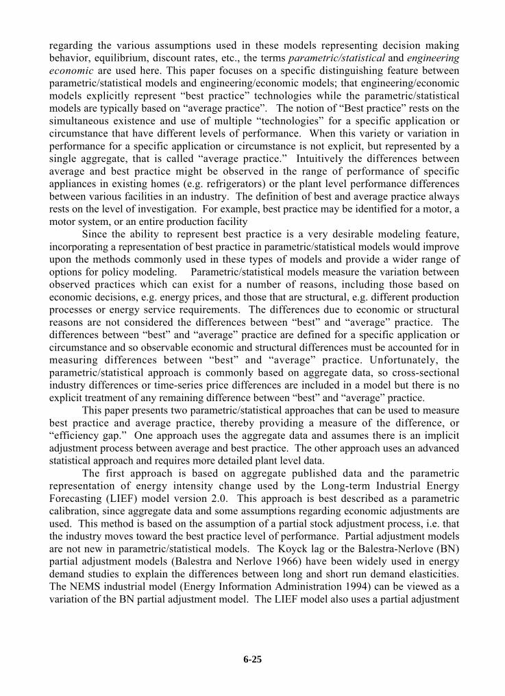
regarding the various assumptions used in these models representing decision makingbehavior, equilibrium, discount rates, etc., the terms parametric/statistical and engineeringeconomic are used here. This paper focuses on a specific distinguishing feature betweenparametric/statistical models and engineering/economic models; that engineering/economicmodels explicitly represent “best practice” technologies while the parametric/statisticalmodels are typically based on “average practice”. The notion of “Best practice” rests on thesimultaneous existence and use of multiple “technologies” for a specific application orcircumstance that have different levels of performance. When this variety or variation inperformance for a specific application or circumstance is not explicit, but represented by asingle aggregate, that is called “average practice.” Intuitively the differences betweenaverage and best practice might be observed in the range of performance of specificappliances in existing homes (e.g. refrigerators) or the plant level performance differencesbetween various facilities in an industry. The definition of best and average practice alwaysrests on the level of investigation. For example, best practice may be identified for a motor, amotor system, or an entire production facility

Since the ability to represent best practice is a very desirable modeling feature,incorporating a representation of best practice in parametric/statistical models would improveupon the methods commonly used in these types of models and provide a wider range ofoptions for policy modeling. Parametric/statistical models measure the variation betweenobserved practices which can exist for a number of reasons, including those based oneconomic decisions, e.g. energy prices, and those that are structural, e.g. different productionprocesses or energy service requirements. The differences due to economic or structuralreasons are not considered the differences between “best” and “average” practice. Thedifferences between “best” and “average” practice are defined for a specific application orcircumstance and so observable economic and structural differences must be accounted for inmeasuring differences between “best” and “average” practice. Unfortunately, theparametric/statistical approach is commonly based on aggregate data, so cross-sectionalindustry differences or time-series price differences are included in a model but there is noexplicit treatment of any remaining difference between “best” and “average” practice.

This paper presents two parametric/statistical approaches that can be used to measurebest practice and average practice, thereby providing a measure of the difference, or“efficiency gap.” One approach uses the aggregate data and assumes there is an implicitadjustment process between average and best practice. The other approach uses an advancedstatistical approach and requires more detailed plant level data.

The first approach is based on aggregate published data and the parametricrepresentation of energy intensity change used by the Long-term Industrial EnergyForecasting (LIEF) model version 2.0. This approach is best described as a parametriccalibration, since aggregate data and some assumptions regarding economic adjustments areused. This method is based on the assumption of a partial stock adjustment process, i.e. thatthe industry moves toward the best practice level of performance. Partial adjustment modelsare not new in parametric/statistical models. The Koyck lag or the Balestra-Nerlove (BN)partial adjustment models (Balestra and Nerlove 1966) have been widely used in energydemand studies to explain the differences between long and short run demand elasticities.The NEMS industrial model (Energy Information Administration 1994) can be viewed as avariation of the BN partial adjustment model. The LIEF model also uses a partial adjustment

6-25

framework, but the adjustment can vary over time since it is explicitly interpreted as thepenetration of energy efficient technologies.

The second approach requires plant level data and applies a stochastic frontierregression analysis to energy intensity used by the ENERGY STAR Industrial EnergyPerformance Indicator (EPI). Stochastic frontier regression analysis separates the energyintensity into three components, systematic effects, inefficiency, and statistical (random)error (Aigner, Lovell et al. 1977). This approach is derived from the production efficiencyliterature, which examines inefficiency in production and can be traced back to (Farrell1957). (Huntington 1995) provides a review of the production efficiency approach in thecontext of energy. (Green 1993) reviews the statistical methods applied to estimatingparametric frontier models, including the stochastic frontier.

The paper outlines both approaches, presents an empirical example, summarizes thedata used and discusses the results. The benefits of each of the two approaches, with a focuson the tradeoffs, are presented in the conclusion.

Long-term Industrial Energy Forecasting (LIEF) model

This section describes the aggregate industry model approach used to estimate the gapbetween of average and best practice energy intensity. Results are given for 12 industrysectors using the LIEF model.

Approach

The first approach is based on aggregate data derived from published sources and theparametric representation of energy intensity change used by the Long-term IndustrialEnergy Forecasting (LIEF) model (Ross, Thimmapuran et al. 1993). This approach is bestdescribed as a parametric calibration. Using 1990 as a base year in LIEF, the trends inaggregate energy intensity of 12 industry sectors from 1990 to 1998 are examined. Anestimate of the gap between average and best practice energy intensity in 1990 can be madewhich rationalizes the actual 1998 intensity within the LIEF model framework. The LIEFmodel assumes that the ideal energy intensity is an industry specific function of prices;therefore the gap between average and best practice also varies with prices.

The basic form of the LIEF model is represented by two relationships. The first is aparametric conservation supply curve (CSC) with an exogenous trend that represents theidealized energy intensity in year t, et* (eq. 1). The parameters _ and _ represent the slope ofthe CSC and the exogenous rate of change, respectively. The best practice energy intensity iscomputed by the CSC for electricity and fossil fuels based on the market prices and thecapital recovery factor.2

te

CRFP

CRFP

ti

t

ti

b

a-

˙˙˙

˚

˘

ÍÍÍ

Î

È

=

0

0,

,

*0

e*e (1)

2 The subscript i in the price term denotes the energy type, either fossil fuel or electric. The subscript issuppressed on the realized and idealized energy intensity variables.

6-26

The second is the partial adjustment process that represents the movement of theindustry average energy intensity, et , to approach the best practice energy intensity (eq. 2).

*e1

e)1(et

ett

lbl +-

-= (2)

The ratio of the average energy intensity et to the best practice energy intensity, et*inthe base year, for each industry and energy type, is represented by the Gap parameter, sincee0* (the idealized energy intensity in the base year) is not observable.

( )Gap-= 10

e*0

e (3)

In order to update the base year of the LIEF model from version 1.0 to a new base year inversion 2.0 it is necessary to reexamine the Gap parameter.

Version 2.0 of LIEF uses the same parameters as in LIEF 1.0 to determine what valueof Gap in 1990 would be consistent with observed energy intensities in 1998. In otherwords, given a level of penetration of new energy technology and the historical energy pricepath, what would the Gap have to have been in 1990 to be consistent with the observedenergy intensities in 1998? Initially the CSC slope and exogenous trend parametersremained the same as in LIEF 1.0, but as is explained below the exogenous trend parametersfor electricity had to be adjusted to be more consistent with the trends that become apparentin the eighties and nineties.

The process for benchmarking the Gap parameter in LIEF 2.0 is conceptually simple.A penetration rate of 3% was assumed to apply for the period 1990-1998. This rate is similarto the level of capital turnover and has been used for other studies as a typical rate ofpenetration. Historical energy prices from 1990 to 1998 were used for the CSC, holding theslope of the curve constant. Given the exogenous trends in LIEF a set of Gap parameterswere computed that were consistent with either the actual change from 1990-1998 or theregression growth rate. Since nearly all of the LIEF sectors had exogenous trends towardincreased electricity use, the Gap parameter that would rationalize a decline in intensity wasoften unreasonably large. This led to a re-examination of those trends.

Historically, there was an aggregate trend toward increased electricity used from themid-fifties to the mid-seventies (see figure 1). Even after prices had stopped rising andbegan to fall in the mid-eighties, aggregate electricity use per $ of GDP was flat. While theshift that occurred in the seventies may be seen as a price response, the asymmetry of theresponse may be attributed to electric savings technology that has become incorporated into“business as usual.” Similar patterns can be seen in individual sectors, so a simplifyingassumption that there is no exogenous trend in electric intensity was made.

Data

Data for the manufacturing sectors in LIEF (12 of the 18 total sectors) was updated tothe year 19983. Table 1 provides the stylized facts of the changes in energy intensitybetween 1990 and 1998. The data for energy use is based primarily on the Annual survey ofManufacturing (ASM) with supplemental data from the Manufacturing Energy ConsumptionSurvey. The denominator for energy intensity is value added from the Bureau of LaborStatistics (BLS) input output tables. The choice between economic measures of output, e.g. 3 The dataset is available from the author on request.

6-27

value added, and physical measures, e.g. tons of steel, have been a important issue inindustrial modeling. The choice of value added as the data in LIEF was made for the sake ofconsistency and expediency. The issue of physical output measures is reexamined in the nextsection on the second method for measuring the efficiency gap. The first two rows are theannual average change from the year 1990 to 1998. Although it is the base year of Version1.0 of LIEF and therefore the base year of the update, 1990 may not be a good benchmarkyear. In 1990 there was significant economic slowdown. Historically, years with low levelsof capacity utilization have higher energy intensity, particularly for energy intensive sectors.To the extent that the year 1990 lies above the long term trend for energy intensity, using thetwo endpoint years may overstate the change in intensity for that sector. The second tworows give the annual average change based on a simple trend regression from 1986 to 19984.In 1986, energy prices dropped significantly, so this period represents a new period forenergy markets, relative to the previous years. For many sectors the regression line providesa more conservative estimate of the changes in energy intensity. What is of particular note isthat both the 1990-1998 and the trend line growth rates for electricity all are lower than thehistorical trends incorporated in LIEF 1.0. In many cases, the sign has reversed from positiveto a negative, indicating a reversal in the growth in electric intensity (i.e. electrification)toward energy savings.

Figure 1. Trends in Aggregate Manufacturing Electricity Intensity and Price

0.40

0.60

0.80

1.00

1.20

1.40

1.60

1955 1960 1965 1970 1975 1980 1985 1990 1995 2000

Year

Inte

nsi

ty (

1973

=1.

0)

0

1

2

3

4

5

6

7

8

9

10

Pri

ce (

1992

Co

nst

ant

cen

ts p

er K

wh

)

kWh / GDP Electric price (Cents per kWh)

Results

Given no exogenous trends in electric intensity in LIEF, the Ga0 parameter was againcomputed as described above. This resulted in Gap estimates of much more reasonablemagnitude. These estimates, which are denoted as Gap1990 are given in table 2. Many ofthese estimates are similar in magnitude with those from LIEF version 1.0. The three largest 4 For a few sectors, a ten year trend was used, due to concerns about the quality of the aggregate time series.

6-28

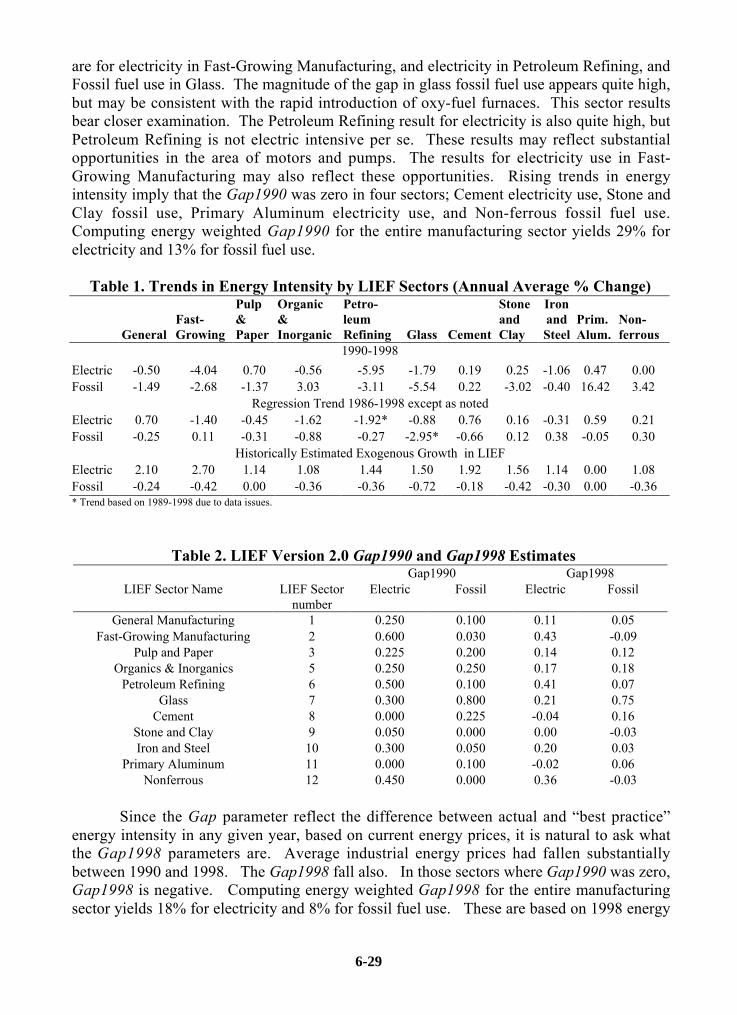
are for electricity in Fast-Growing Manufacturing, and electricity in Petroleum Refining, andFossil fuel use in Glass. The magnitude of the gap in glass fossil fuel use appears quite high,but may be consistent with the rapid introduction of oxy-fuel furnaces. This sector resultsbear closer examination. The Petroleum Refining result for electricity is also quite high, butPetroleum Refining is not electric intensive per se. These results may reflect substantialopportunities in the area of motors and pumps. The results for electricity use in Fast-Growing Manufacturing may also reflect these opportunities. Rising trends in energyintensity imply that the Gap1990 was zero in four sectors; Cement electricity use, Stone andClay fossil use, Primary Aluminum electricity use, and Non-ferrous fossil fuel use.Computing energy weighted Gap1990 for the entire manufacturing sector yields 29% forelectricity and 13% for fossil fuel use.

Table 1. Trends in Energy Intensity by LIEF Sectors (Annual Average % Change)

GeneralFast-Growing

Pulp&Paper

Organic&Inorganic

Petro-leumRefining Glass Cement

StoneandClay

IronandSteel

Prim.Alum.

Non-ferrous

1990-1998

Electric -0.50 -4.04 0.70 -0.56 -5.95 -1.79 0.19 0.25 -1.06 0.47 0.00Fossil -1.49 -2.68 -1.37 3.03 -3.11 -5.54 0.22 -3.02 -0.40 16.42 3.42

Regression Trend 1986-1998 except as notedElectric 0.70 -1.40 -0.45 -1.62 -1.92* -0.88 0.76 0.16 -0.31 0.59 0.21Fossil -0.25 0.11 -0.31 -0.88 -0.27 -2.95* -0.66 0.12 0.38 -0.05 0.30

Historically Estimated Exogenous Growth in LIEFElectric 2.10 2.70 1.14 1.08 1.44 1.50 1.92 1.56 1.14 0.00 1.08Fossil -0.24 -0.42 0.00 -0.36 -0.36 -0.72 -0.18 -0.42 -0.30 0.00 -0.36* Trend based on 1989-1998 due to data issues.

Since the Gap parameter reflect the difference between actual and “best practice”energy intensity in any given year, based on current energy prices, it is natural to ask whatthe Gap1998 parameters are. Average industrial energy prices had fallen substantiallybetween 1990 and 1998. The Gap1998 fall also. In those sectors where Gap1990 was zero,Gap1998 is negative. Computing energy weighted Gap1998 for the entire manufacturingsector yields 18% for electricity and 8% for fossil fuel use. These are based on 1998 energy

Table 2. LIEF Version 2.0 Gap1990 and Gap1998 EstimatesGap1990 Gap1998

LIEF Sector Name LIEF Sectornumber

Electric Fossil Electric Fossil

General Manufacturing 1 0.250 0.100 0.11 0.05Fast-Growing Manufacturing 2 0.600 0.030 0.43 -0.09

Pulp and Paper 3 0.225 0.200 0.14 0.12Organics & Inorganics 5 0.250 0.250 0.17 0.18

Petroleum Refining 6 0.500 0.100 0.41 0.07Glass 7 0.300 0.800 0.21 0.75

Cement 8 0.000 0.225 -0.04 0.16Stone and Clay 9 0.050 0.000 0.00 -0.03Iron and Steel 10 0.300 0.050 0.20 0.03

Primary Aluminum 11 0.000 0.100 -0.02 0.06Nonferrous 12 0.450 0.000 0.36 -0.03

6-29

prices. EIA forecasts fossil fuel prices to quickly return to 1990 levels, but electricity pricesare expected to remain low. In a general sense, this price outlook suggests that a typical gapin manufacturing in the next ten years will be in the “mid-teens.” However, individualsectors may vary substantially from that average.

Energy Performance Indicator (EPI)

This section describes the plant-level, frontier regression model approach used toestimate the distribution of energy efficiency. Examples are given from the ENERGY STAR

energy performance indicator for breweries and motor vehicle assembly.

Approach

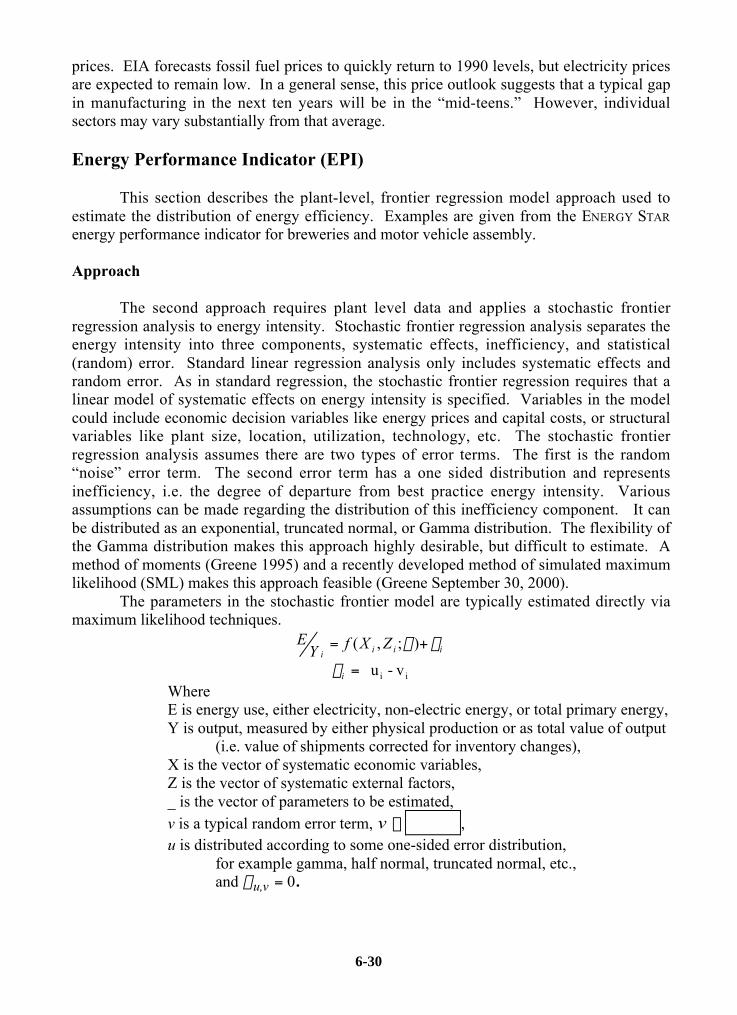
The second approach requires plant level data and applies a stochastic frontierregression analysis to energy intensity. Stochastic frontier regression analysis separates theenergy intensity into three components, systematic effects, inefficiency, and statistical(random) error. Standard linear regression analysis only includes systematic effects andrandom error. As in standard regression, the stochastic frontier regression requires that alinear model of systematic effects on energy intensity is specified. Variables in the modelcould include economic decision variables like energy prices and capital costs, or structuralvariables like plant size, location, utilization, technology, etc. The stochastic frontierregression analysis assumes there are two types of error terms. The first is the random“noise” error term. The second error term has a one sided distribution and representsinefficiency, i.e. the degree of departure from best practice energy intensity. Variousassumptions can be made regarding the distribution of this inefficiency component. It canbe distributed as an exponential, truncated normal, or Gamma distribution. The flexibility ofthe Gamma distribution makes this approach highly desirable, but difficult to estimate. Amethod of moments (Greene 1995) and a recently developed method of simulated maximumlikelihood (SML) makes this approach feasible (Greene September 30, 2000).

The parameters in the stochastic frontier model are typically estimated directly viamaximum likelihood techniques.

iiiiZXfY

E eb += );,(

e i = u - vi i

WhereE is energy use, either electricity, non-electric energy, or total primary energy,Y is output, measured by either physical production or as total value of output

(i.e. value of shipments corrected for inventory changes),X is the vector of systematic economic variables,Z is the vector of systematic external factors,_ is the vector of parameters to be estimated,v is a typical random error term, v ~ , u is distributed according to some one-sided error distribution,

for example gamma, half normal, truncated normal, etc.,and su,v = 0.

6-30

The flexibility of the Gamma distribution makes this approach highly desirable, butdifficult to estimate. The Gamma distribution can generate the exponential distribution as aspecial case, as well as a more ‘general’ one-sided distributions (see figure 1). There are nomaximum likelihood techniques when u is distributed following a gamma distribution, but aconsistent moments estimator exists. Conceptually, the regression is shifted so that (nearly)all the residuals are positive and the parameters of the normal error and gamma efficiencydistributions are computed from those residuals. The method of moments computes theparameters of the gamma distribution f(u) and provides is a consistent adjustment to thelinear regression intercept, a, based on the residuals, ei.

Figure 2. Example of Gamma Density

Â=

-=

-=

=

--=

>G= --

i

rir

v

PuP

eNm

Pa

Pm

mP

mmm

PuuePuf

)/1(

ˆ/ˆˆ

ˆ/ˆˆ

2/ˆˆ

)3/(3ˆ

0,,,)](/[)(

22

2

33

2243

1

qa

qs

q

q

qq q

A recently developed method of SML makes substantial improvement on the methodof moments, since the parameters of the gamma distribution are simultaneously estimatedwith the systematic effects, _. We used both the moments estimator and SML5. We reportexamples of both approaches below.

Data

This analysis uses confidential plant level data from two sources; LongitudinalResearch Database (LRD) maintained by the Center for Economic Studies (CES), U.S.Bureau of the Census and data provided to Argonne National Laboratory by companiesparticipating in the U.S. Environmental Protection Agency (EPA) ENERGY STAR automobilemanufacturing industry focus6. The LRD includes the non-public, plant-level data which isthe basis of the government published statistics on manufacturing. CES has constructed apanel of plant-level data from the Annual Survey of Manufactures (ASM) and the Census ofManufacturers (CM). The LRD includes economic activity, e.g. labor, energy, plant andequipment, and materials costs and total shipment value of output, for a sample of plantsduring the survey years and complete coverage during the years of the economic census.7

5 The simulated maximum likelihood has only recently be made operational in the LIMDEP statistical package,so this paper only presents the SML for the auto industry data.6 The auto manufacturing industry data is proprietary business information and was provided to ANL under anon-disclosure agreement with the respective companies.7 Those are the years ending in ‘2’ or ‘7’, e.g. 1982 or 1997.

Density of Inefficiency Component

U

.2

.4

.6

.8

1.0

.0 .4 .8 1.2 1.6 2.0.0

GAMMAEXPON

f(u)

6-31

Under Title 13 of the U.S. Code this data is confidential, however CES allows academic andgovernment researchers with “Specially Sworn Status” to access these confidential micro-data under its research associate program. The confidentiality restrictions prevent thedisclosure of any information that would allow for the identification of a specific plant orfirm’s activities. Aggregate figures or statistical coefficients that do not reveal the identity ofindividual establishments or firms can be released publicly. The ability to use plant leveldata, rather than aggregate data, significantly enhances the information that can be obtainedabout economic performance, particularly when examining the issue of energy efficiency.

In the examples presented below, the results for breweries, NAICS code 312120 arebased on the Census LRD data and the results for motor vehicle assembly are from NAICScode 33611, 336112, and 336120, based on the Census LRD data (see table 3) and also ondata provided directly from four manufacturing companies with operations in the UnitedStates (see table 4).

Table 3. Sample Means for Brewery EPI($ and physical units in thousands)

Variable Sample meanNumber of plants 42total value of shipments $ 365,689Production (thousand barrels) 4,408Fuel costs $ 2,374Fuel mMBTU (thousand) 618,394electricity costs $ 3,353KWH (thousand) 63,576

Table 4. Sample Means for Motor Vehicle Assembly EPI

The choice of the variables in the X vector include energy prices, plant scale(measured by output), and other input/output ratios, e.g. capital, materials, labor etc. Sinceenergy consumption may be influenced by climate, as well as production activity, state leveldata on heating and cooling degree days are included in the energy intensity regressions inthe Z vector. This data is matched to the plant location. Plants that manufacture certainenergy intensive inputs, rather than purchase them will have a different pattern of efficientenergy use. The level of upstream integration in motor vehicle assembly was initiallymeasured by the fraction of material costs for stampings and engines. For breweries, thosethan manufacture malt from grain were similarly identified by the share of costs.

The data from the four automotive manufacturing companies was provided after areview of the initial results (described below). This data was more limited in scope, butincluded numbers of vehicle produced, plant capacity, electricity and non-electric energyconsumption. Plants with upstream parts operations, e.g. stamping and engines, had the

Variable Sample meanKwh (thousands) 156,641Fuel use (mMBTU) 1,273,120Total site energy (mMBTU) 1,783,842Production (thousands vehicles) 227,615Capacity (thousands vehicles) 285,751Heating degree days 4,970Number of plant years 139

6-32

energy use for those parts of the plant subtracted from the plant total. In principle, thisallows a more direct comparison of energy use in assembly plants8.

Results

Initial model results for energy intensity equations for both sectors and two forms ofenergy, electricity and non-electric energy, principally purchased fossil fuels, were cleared byCensus for public review. The functional form was a generalized quadratic linear model.Cross-product and squared terms were evaluated, but were rarely significant.

To assist the review a spreadsheet was constructed to display the gamma density anddistribution functions for the parameters that were estimated, evaluated at user selectedvalues of the X and Z vectors. This aided in comparing the magnitude of the systematiceffects (changes in X and Z) with the gamma efficiency distribution by graphicallydisplaying the results. The spreadsheet was provided to energy managers from companies inthe brewery and auto assembly sectors. Examples of the spreadsheets are shown in figures 3and 4 for the brewery and auto assembly sectors, respectively, with data based on the samplemeans. The energy managers were allowed to input data for their own plants and thenprovide comments.

During the review process the point was made shipment value of production mightnot be an appropriate measure of output. This question of whether to use physical units(tons, barrels, etc) instead of economic units (total value of production, value added, etc.) hasbeen well studied in analysis of energy intensive industries (Freeman, Niefer et al. 1997). Inparticular the use of physical units are useful of international comparisons (Battles 1996)because of difficulties over exchange rates or purchasing power parity. In the case ofbreweries and motor vehicles the issue is that product pricing in these industries reflect anumber of market characteristics, including oligopoly-pricing, rebates, cross-subsidizationetc. such that value of production might not be a good indicator of energy intensity. Forbreweries we constructed a physical measure of production, gallons of malt beverages, usingdetailed Census product code data which reports shipments identified by packaging type(cans, bottles, etc) and size. We compared this estimate (5.7 billion gallons) to the totalindustry gallons of production published by the Bureau of Alcohol, Tobacco, and Firearms(6.2 billion) and determined that it was consistent9. For automobile manufacture, theparticipating companies provided plant level production and energy data.

The re-estimated models illustrate the difference that this price variation makes in theestimates of the efficiency distribution. Figure 5 shows a near exponential distribution for theelectricity output ratio when production is measured in barrels. A similar figure 6 shows anear exponential distribution for the total site energy per vehicle. The results from the autoassembly analysis are discussed in more detail.

8 For the purposes of this paper “assembly” encompasses painting, body weld, and the final assembly process.9 We include only large breweries in our analysis. Small breweries produced 9% of the total value of output in1997, which is consistent with the differences in physical volume that we estimated.

6-33

Figure 3. Breweries Model Spreadsheet Figure 4 Motor Vehicle Assembly Model Spreadsheet

Plant Characteristics

SIC Code:

5-digit Zip Code: 10101

General Location: New York, NY 1096 4805

Operating CharacteristicsTotal Value of Plant Output ($): $370,000,000 A

Total Annual Material Cost ($): $150,000,000 B

Malt Annual Material Cost ($): $18,000,000 C 12.00%

Non-malted Grain Annual Material Cost ($): $1,500,000 D 1.00%

Annual Energy ConsumptionElectricity Gas Distillate Oil Residual Oil Coal

Select Units

E Annual Consumption 63,000,000 600,000

F Annual Cost 3,000,000 2,500,000

Unit Cost ($/unit) 0.048 4.17

ResultsEfficient Plant

Energy Performance Indicator (Electricity) 75 (1 to 100)

Energy Performance Indicator (non-Elec Fuels) 75 (1 to 100)

Annual Energy Cost ($/year) $4,445,252

Electric Output Ratio (kWh/$ product) 0.1476 (see Table-1)

Fossil Fuel Output Ratio (mMBtu/$1000 product) 1.2370 (see Table-2)

Total Site Energy (mMBtu/year) 635,051

CO2 Emissions Equivalent (Lbs/year) 132,384,139

Table-1 (Electricity) Table-2 (non-Electric Fuels)

$5,519,083 $5,500,000

50 48

Plant Energy Performance Indicator05/15/2002

Average Plant Your Plant

Material Cost Share

Cooling Degree Days Heating Degree Days

164,363,898 163,795,596

54

814,956

50

807,957

1.6120 1.6446

0.1766 0.1727

kWH mMBtu mMBtu Gallons Short Tons

2082 (Malt Beverages)

- 1.00 2.00 3.00 4.00 5.00mMBtu per thousand$ of Production

Pla

nt

Fre

qu

en

cy

0%

10%

20%

30%

40%

50%

60%

70%

80%

90%

100%

En

erg

y P

erf

orm

an

ce

In

dic

ato

rFrequency

Cumulative

Your Plant

0.00 0.10 0.20 0.30 0.40 0.50

kWh per $ of production

Pla

nt

Fre

qu

en

cy

0%

10%

20%

30%

40%

50%

60%

70%

80%

90%

100%

En

erg

y P

erf

orm

an

ce

In

dic

ato

r

Frequency

Cumulative

Your Plant

Plant Characteristics

SIC Code:

5-digit Zip Code: 10101

General Location: New York, NY 1096 4805

Operating CharacteristicsTotal Value of Plant Output ($): $3,000,000,000 A

Total Annual Material Cost ($): $2,000,000,000 B

Automotive Stamping Annual Material Cost ($): $180,000,000 C 9.00%

Gas Engines & Parts Annual Material Cost ($): $300,000,000 D 15.00%

Painting Annual Material Cost ($): $20,000,000 E 1.00%

Drive Train & Parts Annual Material Cost ($): $250,000,000 F 12.50%

Annual Energy ConsumptionElectricity Gas Distillate Oil Residual Oil Coal

Select Units

G Annual Consumption 162,715,141 1,028,690

H Annual Cost 8,034,483 4,047,090

Unit Cost 0.0494 3.93

ResultsEfficient Plant

Energy Performance Indicator (Electricity) 75 (1 to 100)

Energy Performance Indicator (non-Elec Fuels) 75 (1 to 100)

Annual Energy Cost ($/year) $11,087,757

Electric Output Ratio (kWh/$ product) 0.049 (see Table-1)

Fossil Fuel Output Ratio (mMBtu/ $1,000 product) 0.34 (see Table-2)

Total Site Energy, All Fuels (mMBtu/year) 1,159,645

Estimated CO2 Emissions (Tons/year) 166,632

Table-1 (Electricity) Table-2 (Fossil Fuels)

Plant Energy Performance Indicator05/20/2002

213,558 181,568

66

1,028,690

Average Plant Your Plant

50

1,406,638

0.065 0.055

0.41 0.35

Material Cost Share

Cooling Degree Days Heating Degree Days

$14,210,225 $12,081,573

50 74

kWH mMBtu Gallons Gallons Short Tons

3711 (MOTOR VEHICLE ASSEMBLY)

0.20 0.40 0.60 0.80 1.00 1.20 1.40mMBtu per $1,000 of Production

Pla

nt

Fre

qu

en

cy

0%

10%

20%

30%

40%

50%

60%

70%

80%

90%

100%

En

erg

y P

erf

orm

an

ce

In

dic

ato

r

Frequency

Cumulative

Your Plant

0.010 0.060 0.110 0.160 0.210

kWh per $ of production

Pla

nt

Fre

qu

en

cy

0%

10%

20%

30%

40%

50%

60%

70%

80%

90%

100%

En

erg

y P

erf

orm

an

ce

In

dic

ato

r

Frequency

Cumulative

Your Plant

6-34

Figure 5. Efficiency Distribution for Electricity per Barrel

10.00 11.00 12.00 13.00 14.00 15.00 16.00 17.00 18.00 19.00 20.00

kWh per barrel of beer produced

Pla

nt

Fre

qu

en

cy

0%

10%

20%

30%

40%

50%

60%

70%

80%

90%

100%

Pe

rce

nti

lePlant Size 9 Million Gallons per year

75% percentile - 12.3 KWh per barrel

50% percentile - 12.9 kWh per barrel

Figure 6. Efficiency Distributions for Total Site Energy per Vehicle

-

0.10

0.20

0.30

0.40

0.50

0.60

0.70

0.80

0 1 2 3 4 5 6 7 8 9 10 11 12 13 14 15 16 17 18 19 20 21 22 23 24 25 26 27

Site energy per vehicle

0%

10%

20%

30%

40%

50%

60%

70%

80%

90%

100%

5.4

244

100%Utilization rate

Capacity (thousand of vehicles)

75% Percentile Score

50% Percentile Score

million BTU

6.1 million BTU

The final EPI model for motor vehicle assembly was based on 139 plant years of datafrom four motor vehicle manufacturing companies with assembly plants in the U.S. All fourof the companies provided data for each of their plants in operation in the U.S. Twocompanies provided data for each plant for 4 years (1997-2000), while the other twocompanies provided data for three years (1999-2001). A more balance panel would havebeen desirable. The final model estimated was

ii542

321 v-uln ++++++= TRCVANHDDUtilUtilcapAYE

ibbbbb

WhereE = total site energy use in mMBTU (1 kwh=3412BTU)Y = number of vehicles produced

6-35

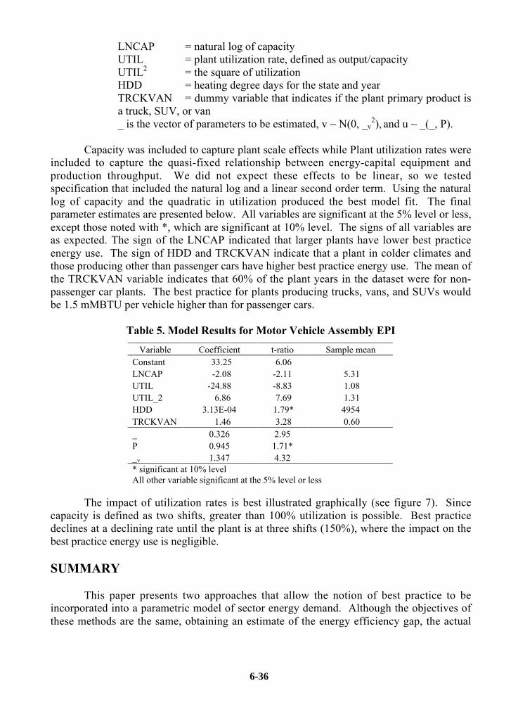
LNCAP = natural log of capacityUTIL = plant utilization rate, defined as output/capacityUTIL2 = the square of utilizationHDD = heating degree days for the state and yearTRCKVAN = dummy variable that indicates if the plant primary product isa truck, SUV, or van_ is the vector of parameters to be estimated, v ~ N(0, _v

2), and u ~ _(_, P).

Capacity was included to capture plant scale effects while Plant utilization rates wereincluded to capture the quasi-fixed relationship between energy-capital equipment andproduction throughput. We did not expect these effects to be linear, so we testedspecification that included the natural log and a linear second order term. Using the naturallog of capacity and the quadratic in utilization produced the best model fit. The finalparameter estimates are presented below. All variables are significant at the 5% level or less,except those noted with *, which are significant at 10% level. The signs of all variables areas expected. The sign of the LNCAP indicated that larger plants have lower best practiceenergy use. The sign of HDD and TRCKVAN indicate that a plant in colder climates andthose producing other than passenger cars have higher best practice energy use. The mean ofthe TRCKVAN variable indicates that 60% of the plant years in the dataset were for non-passenger car plants. The best practice for plants producing trucks, vans, and SUVs wouldbe 1.5 mMBTU per vehicle higher than for passenger cars.

Table 5. Model Results for Motor Vehicle Assembly EPI

The impact of utilization rates is best illustrated graphically (see figure 7). Sincecapacity is defined as two shifts, greater than 100% utilization is possible. Best practicedeclines at a declining rate until the plant is at three shifts (150%), where the impact on thebest practice energy use is negligible.

SUMMARY

This paper presents two approaches that allow the notion of best practice to beincorporated into a parametric model of sector energy demand. Although the objectives ofthese methods are the same, obtaining an estimate of the energy efficiency gap, the actual

Variable Coefficient t-ratio Sample meanConstant 33.25 6.06LNCAP -2.08 -2.11 5.31UTIL -24.88 -8.83 1.08UTIL_2 6.86 7.69 1.31HDD 3.13E-04 1.79* 4954TRCKVAN 1.46 3.28 0.60_ 0.326 2.95P 0.945 1.71*_v 1.347 4.32* significant at 10% levelAll other variable significant at the 5% level or less

6-36

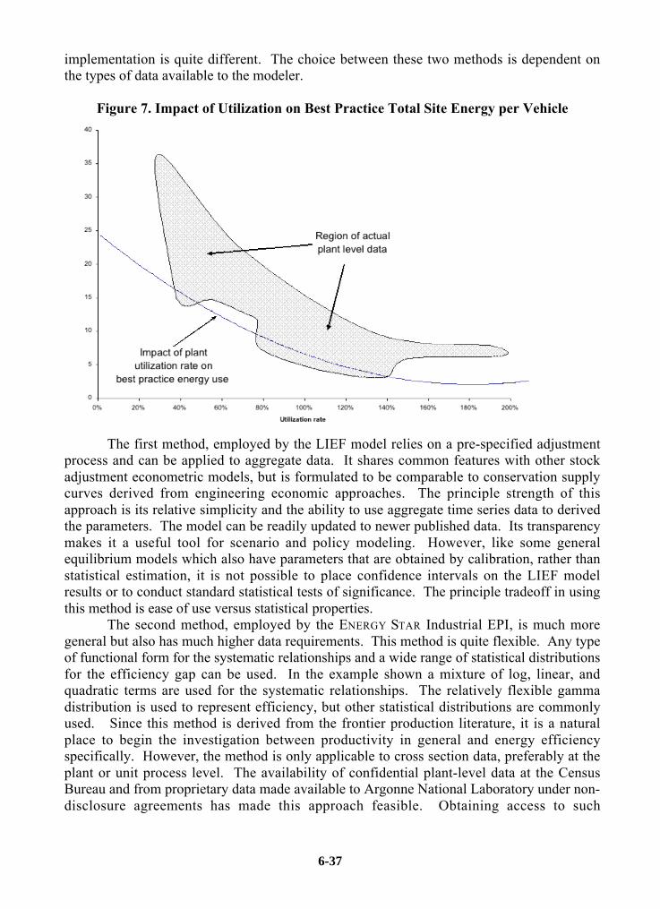
implementation is quite different. The choice between these two methods is dependent onthe types of data available to the modeler.

Figure 7. Impact of Utilization on Best Practice Total Site Energy per Vehicle

The first method, employed by the LIEF model relies on a pre-specified adjustmentprocess and can be applied to aggregate data. It shares common features with other stockadjustment econometric models, but is formulated to be comparable to conservation supplycurves derived from engineering economic approaches. The principle strength of thisapproach is its relative simplicity and the ability to use aggregate time series data to derivedthe parameters. The model can be readily updated to newer published data. Its transparencymakes it a useful tool for scenario and policy modeling. However, like some generalequilibrium models which also have parameters that are obtained by calibration, rather thanstatistical estimation, it is not possible to place confidence intervals on the LIEF modelresults or to conduct standard statistical tests of significance. The principle tradeoff in usingthis method is ease of use versus statistical properties.

The second method, employed by the ENERGY STAR Industrial EPI, is much moregeneral but also has much higher data requirements. This method is quite flexible. Any typeof functional form for the systematic relationships and a wide range of statistical distributionsfor the efficiency gap can be used. In the example shown a mixture of log, linear, andquadratic terms are used for the systematic relationships. The relatively flexible gammadistribution is used to represent efficiency, but other statistical distributions are commonlyused. Since this method is derived from the frontier production literature, it is a naturalplace to begin the investigation between productivity in general and energy efficiencyspecifically. However, the method is only applicable to cross section data, preferably at theplant or unit process level. The availability of confidential plant-level data at the CensusBureau and from proprietary data made available to Argonne National Laboratory under non-disclosure agreements has made this approach feasible. Obtaining access to such

6-37

confidential data can be very time consuming. The process to obtain access approval to plantlevel data at the Census is very rigorous. Even after approval is obtained, Census data canonly be accessed at a limited number of secure research data centers. For researchers whoare willing to clear these hurdles, there are benefits to this approach in terms of statisticalrigor and model detail.

Regardless of the data and the choice between these methods, this paper illustrates theparametric/statistical models need not be based solely concepts of average practice.Parametric/statistical models can be used to represent notions of best practice technologiesand estimate the efficiency gap. As the parametric/statistical methods presented in thispaper are put into more widespread use, the “Gap” between parametric/statistical andengineering economics models may narrow as well.

References

Aigner, D., C. A. K. Lovell, et al. (1977). "Formulation and Estimation of Stochastic FrontierProduction Function Models." Journal of Econometrics 6(1): 53-66.

Balestra, P. and M. Nerlove (1966). "Pooling Cross Section and Time Series Data in theEstimation of a Dynamic Model: The Demand for Natural Gas." Econmetrica 3(July):585-612.

Battles, S. (1996). Measuring Energy Efficiency in the United States Industrial Sector.Workshop on Methodologies for International Comparisons of Industrial EnergyEfficiency, Vancouver, BC, CIEEDAX/Simon Fraser University.

Energy Information Administration (1994). NEMS Industrial Module Documentation Report,U.S. Department of Energy.

Farrell, M. J. (1957). "The Measurement of Productive Efficiency." Journal of the RoyalStatistical Society Series A, General(120, part 3): 253-281.

Freeman, S. L., M. J. Niefer, et al. (1997). "Measuring industrial energy intensity: practicalissues and problems." Energy Policy 25(7-9): 703-714.

Green, W. (1993). The Econometric Approach to Efficiency Analysis. The Measurement ofProductive Efficiency: Techniques and Applications. H. Fried, C. A. K. Lovell and S.Schmidt. New York, Oxford University Press: 68-119.

Greene, W. (1995). LIMDEP Version 7.0 User Manual. Plainview, NY, EconometricSoftware.

Greene, W. H. (September 30, 2000). Simulated Likelihood Estimation of the Normal-Gamma Stochastic Frontier Function. New York University Economics departmentworking paper.

Huntington, H. (1995). "Been Top Down So Long It Looks Like Bottom Up." Energy.

Ross, M., P. Thimmapuran, et al. (1993). Long-Term Industrial Energy Forecasting (LIEF)Model (18-Sector Version), Argonne National Laboratory.

6-38