Tutorial on Gravitational Pendulum Theory Applied

to Seismic Sensing of Translation and Rotation

by Randall D. Peters

Abstract Following a treatment of the simple pendulum provided in Appendix A,a rigorous derivation is given first for the response of an idealized rigid compoundpendulum to external accelerations distributed through a broad range of frequencies. Itis afterward shown that the same pendulum can be an effective sensor of rotation, ifthe axis is positioned close to the center of mass.

Introduction

When treating pendulum motions involving a noniner-tial (accelerated) reference frame, physicists rarely considerthe dynamics of anything other than a simple pendulum.Seismologists are concerned, however, with both instrumentsmore complicated than the simple pendulum and how suchinstruments behave when their framework experiences accel-eration in the form of either translation or rotation. Thus, Ilook at the idealized compound pendulum as the simplestapproximation to mechanical system dynamics of relevanceto seismology. As compared to a simple pendulum, the prop-erties of a compound pendulum can be radically modifiedaccording to the location of its axis relative to the centerof mass.

Pendulum Theory

The Simple Pendulum

The theory of the simple (mathematical) pendulum isprovided in Appendix A.

Theory of an Exemplary Compound Pendulum

When an external force is applied to an extended objectwhose shape is invariant, it generally causes two responses:a linear acceleration of the center of mass and a rotationalacceleration around the center of mass. For this system, New-ton’s laws of translation and rotation are applied respectivelyto each response. The coupled-equation sets obtained fromthese two forms of the law are then combined to obtain thesingle equation of motion. This method will be used to ana-lyze the compound pendulum described next.

As noted, we are concerned with small displacements,where the drive acceleration is rarely large enough to gener-ate amplitudes in excess of 1 mrad. Thus, the nonlinear in-fluence of the sin θ term is inconsequential; that is, theinstrument is nearly isochronous (sin θ≈ θ and cos θ≈ 1).

Figure 1 shows a pendulum similar to various instru-ments of importance in seismology. It is a true pendulum

in the sense that restoration is due to the gravitational fieldof the Earth at its surface, little g. Some other instrumentscommon in physics and sometimes labeled pendulums donot employ a restore-to-equilibrium torque based on theEarth’s field. For example, restoration in the Michell–Cavendish balance that is used to measure big G (Newtonianuniversal gravitational constant) is provided by the elastictwist of a fiber (TEL-Atomic, Inc., 2008). It is sometimescalled a torsion pendulum. Many seismic instruments arealso called pendulums, even though restoration may bemostly provided by a spring. Two commonly employedspring types are the LaCoste zero-length and the astatic.As discussed in Appendix B, the rotation response at lowfrequencies of a spring-restored oscillator is significantly dif-ferent from that of a gravity-restored pendulum.

While the fiber of the Cavendish balance is secured onlyat the top, other torsion pendulums use a vertical fiber thatis also secured at both ends. The best known example fromseismology is the Wood–Anderson seismograph, used byRichter to define the original earthquake magnitude scale.By means of an adjustable period, a similar instrument canbe configured to operate with large tilt sensitivity (Peters,1990). As with any long-period mechanical oscillator, themaximum period (and the maximum sensitivity) of the tilt-meter is regulated by the integrity of its fiber spring. Accept-able stability against spring creep is difficult to achieve whenthe period is greater than about 30 sec (de Silva, 2007). Acommon seismology instrument for which the challengeto long-period stability is well known is the garden-gate hori-zontal pendulum. Rodgers (1968) recognized its potential fora variety of measurements.

Although the instrument in Figure 1 is idealized in theform of a two-element compound pendulum, it neverthelessis useful for illustrating a variety of important properties. Theprimary idealization is the assumption of a rigid structure.For reasons of material creep, and the placement of massM1 above the axis, real pendulums of this type experiencestructural deformation. In the absence of integrity sufficient

1

Bulletin of the Seismological Society of America, Vol. 99, No. 2B, pp. –, May 2009, doi: 10.1785/0120080163

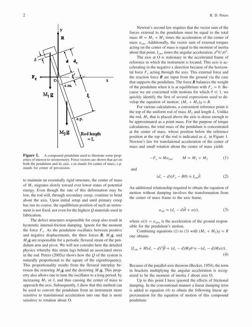
to maintain an essentially rigid structure, the center of massof M1 migrates slowly toward ever lower states of potentialenergy. Even though the rate of this deformation may below, the rod will, through secondary creep, continue to bendabout the axis. Upon initial setup and until primary creephas run its course, the equilibrium position of such an instru-ment is not fixed, not even for the highestQmaterials used infabrication.

The defect structures responsible for creep also result inhysteretic internal-friction damping. Ignore for the momentthe force Fe. As the pendulum oscillates between positiveand negative displacements, the three forces R, M1g, andM2g are responsible for a periodic flexural strain of the pen-dulum arm and pivot. We will not consider here the detailedphysics whereby this strain lags behind an associated stressin the rod. Peters (2005a) shows how the Q of the system isnaturally proportional to the square of the eigenfrequency.This proportionality results from the flexural interplay be-tween the restoring M2g and the destoring M1g. This prop-erty also allows one to tune the oscillator to a long period, byincreasing M1 or δ, and thus causing the center of mass toapproach the axis. Subsequently, I show that this method canbe used to convert the pendulum from an instrument moresensitive to translational acceleration into one that is moresensitive to rotation about O.

Newton’s second law requires that the vector sum of theforces external to the pendulum must be equal to the totalmass M � M1 �M2 times the acceleration of the center ofmass acm. Additionally, the vector sum of external torquesacting on the center of mass is equal to the moment of inertiaabout that point, Icm, times the angular acceleration, d2θ=dt2.

The axis at O is stationary in the accelerated frame ofreference in which the instrument is located. This axis is ac-celerating in the negative x direction because of the horizon-tal force Fe acting through the axis. This external force andthe reaction force R are input from the ground via the casethat supports the pendulum. The force R balances the weightof the pendulum when it is at equilibrium with Fe � 0. Be-cause we are concerned with motions for which θ ≪ 1, wequickly identify the first of several expressions used to de-velop the equation of motion: �M1 �M2�g≈ R.

For various calculations, a convenient reference point isthe top of the uniform rod of mass M2 and length L. Unlikethe rod, M1 that is placed above the axis is dense enough tobe approximated as a point mass. For the purpose of torquecalculations, the total mass of the pendulum is concentratedat the center of mass, whose position below the referenceposition at the top of the rod is indicated as dc in Figure 1.Newton’s law for translational acceleration of the center ofmass and small rotation about the center of mass yields

�Fe ≈Macm; M � M1 �M2 (1)

and

�dc � d��Fe � Rθ�≈ Icm �θ: (2)

An additional relationship required to obtain the equation ofmotion without damping involves the transformation fromthe center of mass frame to the axis frame,

acm ≈ �dc � d��θ� a�t�; (3)

where a�t� � aaxis is the acceleration of the ground respon-sible for the pendulum’s motion.

Combining equations (1) to (3) with �M1 �M2�g � Rone obtains

�Icm �M�dc � d�2��θ� �dc � d�Mgθ≈ ��dc � d�Ma�t�:(4)

Because of the parallel-axis theorem (Becker, 1954), the termin brackets multiplying the angular acceleration is recog-nized to be the moment of inertia I about axis O.

Up to this point I have ignored the effects of frictionaldamping. In the conventional manner a linear damping termis added to equation (4) to obtain the following linear ap-proximation for the equation of motion of this compoundpendulum:

Figure 1. A compound pendulum used to illustrate some prop-erties of interest to seismometry. Force vectors are shown that act onboth the pendulum and its axis. c.m stands for center of mass; c.p.stands for center of percussion.

2 R. D. Peters

�θ� ω0

Q_θ� ω2

0θ≈ �ω20

ga�t�; ω2

0 �M�dc � d�g

I;

dc �M2

L2�M1δ

M: (5)

The equation is seen to be identical to that of the drivensimple pendulum (equation A3, given in Appendix A, exceptwith a drive term added to the right-hand side, and theexpression for its eigenfrequency is considerably morecomplicated).

Radius of Gyration

It is common practice in physics and engineering to ex-press the moment of inertia of a rigid object in terms of alength ρ called the radius of gyration and defined by

I � Mρ2: (6)

In keeping with this convention, we find for the compoundpendulum just described

ρ2 � ρ2cm � L2

�dcL

� d

L

�2

;

ρ2cm � L2

M

�M2

�1

3� dc

L�

�dcL

�2��M1

�dcL

� δL

�2�:

(7)

The distance ξ0 � �dc � d� of axis O above the center ofmass has a conjugate point called the center of percussionthat is located a distance ξ below the center of mass; thesepoints obey the relation

ξ0ξ � ρ2cm: (8)

As demonstrated in textbooks of mechanics (e.g.,Becker, 1954, pp. 213), an impulsive force delivered perpen-dicular to the equilibrated pendulum at the center of per-cussion imparts no motion to the axis. An example of thisphenomenon is the sweet spot of a baseball bat. When theball is hit at that point there is no counter force to the batter’shands. For drive frequencies higher than the eigenfrequency,a sensor located at the center of percussion measures pendu-lum displacement equal in magnitude and π out of phase withthe displacement of sinusoidal ground motion.

Determining the center of percussion allows one to de-fine an effective (i.e., an equivalent simple pendulum) lengthby means of the following relationship:

ξ � ξ0 � Leff ; (9)

where Leff corresponds to the length of a simple pendulumhaving the same period as the compound pendulum. For thepresent compound pendulum

Leff

L�

��dcL

� d

L

�2

�M2

M

�1

3� dc

L�

�dcL

�2�

�M1

M

�dcL

� d

L

�2�=

�dcL

� d

L

�: (10)

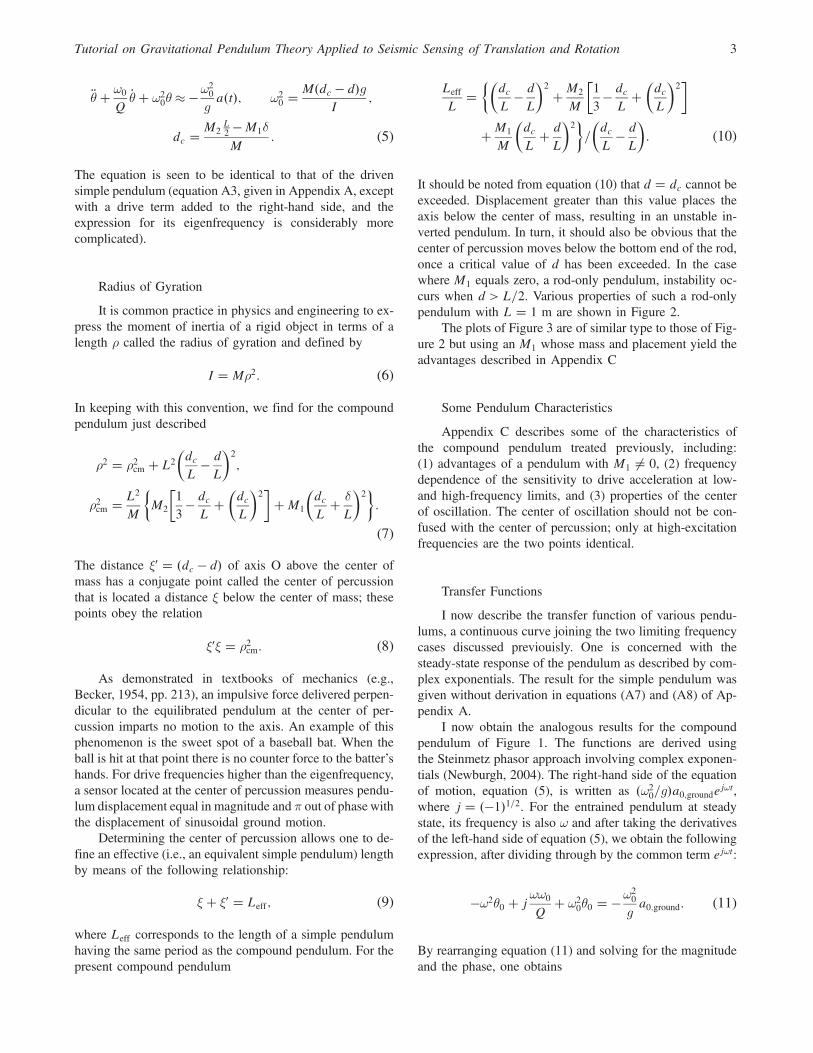
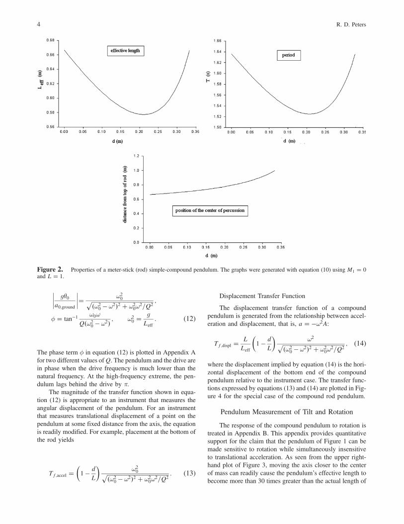
It should be noted from equation (10) that d � dc cannot beexceeded. Displacement greater than this value places theaxis below the center of mass, resulting in an unstable in-verted pendulum. In turn, it should also be obvious that thecenter of percussion moves below the bottom end of the rod,once a critical value of d has been exceeded. In the casewhere M1 equals zero, a rod-only pendulum, instability oc-curs when d > L=2. Various properties of such a rod-onlypendulum with L � 1 m are shown in Figure 2.

The plots of Figure 3 are of similar type to those of Fig-ure 2 but using an M1 whose mass and placement yield theadvantages described in Appendix C

Some Pendulum Characteristics

Appendix C describes some of the characteristics ofthe compound pendulum treated previously, including:(1) advantages of a pendulum with M1 ≠ 0, (2) frequencydependence of the sensitivity to drive acceleration at low-and high-frequency limits, and (3) properties of the centerof oscillation. The center of oscillation should not be con-fused with the center of percussion; only at high-excitationfrequencies are the two points identical.

Transfer Functions

I now describe the transfer function of various pendu-lums, a continuous curve joining the two limiting frequencycases discussed previouisly. One is concerned with thesteady-state response of the pendulum as described by com-plex exponentials. The result for the simple pendulum wasgiven without derivation in equations (A7) and (A8) of Ap-pendix A.

I now obtain the analogous results for the compoundpendulum of Figure 1. The functions are derived usingthe Steinmetz phasor approach involving complex exponen-tials (Newburgh, 2004). The right-hand side of the equationof motion, equation (5), is written as �ω2

0=g�a0;groundejωt,where j � ��1�1=2. For the entrained pendulum at steadystate, its frequency is also ω and after taking the derivativesof the left-hand side of equation (5), we obtain the followingexpression, after dividing through by the common term ejωt:

�ω2θ0 � jωω0

Q� ω2

0θ0 � �ω20

ga0;ground: (11)

By rearranging equation (11) and solving for the magnitudeand the phase, one obtains

Tutorial on Gravitational Pendulum Theory Applied to Seismic Sensing of Translation and Rotation 3

���� gθ0a0;ground

����� ω20�����������������������������������������������

�ω20 � ω2�2 � ω2

0ω2=Q2

p ;

ϕ � tan�1ω0ω

Q�ω20 � ω2� ; ω2

0 �g

Leff: (12)

The phase term ϕ in equation (12) is plotted in Appendix Afor two different values ofQ. The pendulum and the drive arein phase when the drive frequency is much lower than thenatural frequency. At the high-frequency extreme, the pen-dulum lags behind the drive by π.

The magnitude of the transfer function shown in equa-tion (12) is appropriate to an instrument that measures theangular displacement of the pendulum. For an instrumentthat measures translational displacement of a point on thependulum at some fixed distance from the axis, the equationis readily modified. For example, placement at the bottom ofthe rod yields

Tf;accel ��1 � d

L

�ω20�����������������������������������������������

�ω20 � ω2�2 � ω2

0ω2=Q2

p : (13)

Displacement Transfer Function

The displacement transfer function of a compoundpendulum is generated from the relationship between accel-eration and displacement, that is, a � �ω2A:

Tf;displ �L

Leff

�1 � d

L

�ω2�����������������������������������������������

�ω20 � ω2�2 � ω2

0ω2=Q2

p ; (14)

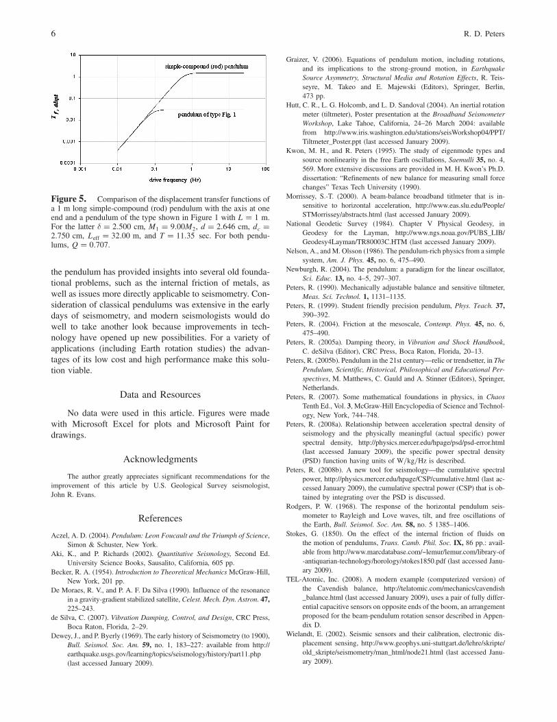
where the displacement implied by equation (14) is the hori-zontal displacement of the bottom end of the compoundpendulum relative to the instrument case. The transfer func-tions expressed by equations (13) and (14) are plotted in Fig-ure 4 for the special case of the compound rod pendulum.

Pendulum Measurement of Tilt and Rotation

The response of the compound pendulum to rotation istreated in Appendix B. This appendix provides quantitativesupport for the claim that the pendulum of Figure 1 can bemade sensitive to rotation while simultaneously insensitiveto translational acceleration. As seen from the upper right-hand plot of Figure 3, moving the axis closer to the centerof mass can readily cause the pendulum’s effective length tobecome more than 30 times greater than the actual length of

Figure 2. Properties of a meter-stick (rod) simple-compound pendulum. The graphs were generated with equation (10) using M1 � 0and L � 1.

4 R. D. Peters

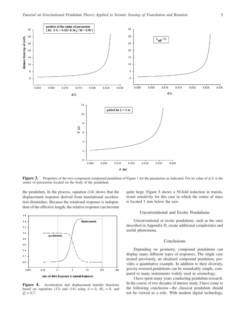
the pendulum. In the process, equation (14) shows that thedisplacement response derived from translational accelera-tion diminishes. Because the rotational response is indepen-dent of the effective length, the relative response can become

quite large. Figure 5 shows a 50-fold reduction in transla-tional sensitivity for this case in which the center of massis located 1 mm below the axis.

Unconventional and Exotic Pendulums

Unconventional or exotic pendulums, such as the onesdescribed in Appendix D, create additional complexities anduseful phenomena.

Conclusions

Depending on geometry, compound pendulums candisplay many different types of responses. The single casetreated previously, an idealized compound pendulum, pro-vides a quantitative example. In addition to their diversity,gravity-restored pendulums can be remarkably simple, com-pared to many instruments widely used in seismology.

I have spent many years conducting pendulum research.In the course of two decades of intense study, I have come tothe following conclusion—the classical pendulum shouldnot be viewed as a relic. With modern digital technology,

Figure 3. Properties of the two-component compound pendulum of Figure 1 for the parameters as indicated. For no value of d=L is thecenter of percussion located on the body of the pendulum.

Figure 4. Acceleration and displacement transfer functionsbased on equations (13) and (14) using d � 0, M1 � 0, andQ � 0:7.

Tutorial on Gravitational Pendulum Theory Applied to Seismic Sensing of Translation and Rotation 5

the pendulum has provided insights into several old founda-tional problems, such as the internal friction of metals, aswell as issues more directly applicable to seismometry. Con-sideration of classical pendulums was extensive in the earlydays of seismometry, and modern seismologists would dowell to take another look because improvements in tech-nology have opened up new possibilities. For a variety ofapplications (including Earth rotation studies) the advan-tages of its low cost and high performance make this solu-tion viable.

Data and Resources

No data were used in this article. Figures were madewith Microsoft Excel for plots and Microsoft Paint fordrawings.

Acknowledgments

The author greatly appreciates significant recommendations for theimprovement of this article by U.S. Geological Survey seismologist,John R. Evans.

References

Aczel, A. D. (2004). Pendulum: Leon Foucault and the Triumph of Science,Simon & Schuster, New York.

Aki, K., and P. Richards (2002). Quantitative Seismology, Second Ed.University Science Books, Sausalito, California, 605 pp.

Becker, R. A. (1954). Introduction to Theoretical Mechanics McGraw-Hill,New York, 201 pp.

De Moraes, R. V., and P. A. F. Da Silva (1990). Influence of the resonancein a gravity-gradient stabilized satellite, Celest. Mech. Dyn. Astron. 47,225–243.

de Silva, C. (2007). Vibration Damping, Control, and Design, CRC Press,Boca Raton, Florida, 2–29.

Dewey, J., and P. Byerly (1969). The early history of Seismometry (to 1900),Bull. Seismol. Soc. Am. 59, no. 1, 183–227: available from http://earthquake.usgs.gov/learning/topics/seismology/history/part11.php(last accessed January 2009).

Graizer, V. (2006). Equations of pendulum motion, including rotations,and its implications to the strong-ground motion, in EarthquakeSource Asymmetry, Structural Media and Rotation Effects, R. Teis-seyre, M. Takeo and E. Majewski (Editors), Springer, Berlin,473 pp.

Hutt, C. R., L. G. Holcomb, and L. D. Sandoval (2004). An inertial rotationmeter (tiltmeter), Poster presentation at the Broadband SeismometerWorkshop, Lake Tahoe, California, 24–26 March 2004: availablefrom http://www.iris.washington.edu/stations/seisWorkshop04/PPT/Tiltmeter_Poster.ppt (last accessed January 2009).

Kwon, M. H., and R. Peters (1995). The study of eigenmode types andsource nonlinearity in the free Earth oscillations, Saemulli 35, no. 4,569. More extensive discussions are provided in M. H. Kwon’s Ph.D.dissertation: “Refinements of new balance for measuring small forcechanges” Texas Tech University (1990).

Morrissey, S.-T. (2000). A beam-balance broadband titlmeter that is in-sensitive to horizontal acceleration, http://www.eas.slu.edu/People/STMorrissey/abstracts.html (last accessed January 2009).

National Geodetic Survey (1984). Chapter V Physical Geodesy, inGeodesy for the Layman, http://www.ngs.noaa.gov/PUBS_LIB/Geodesy4Layman/TR80003C.HTM (last accessed January 2009).

Nelson, A., andM. Olsson (1986). The pendulum-rich physics from a simplesystem, Am. J. Phys. 45, no. 6, 475–490.

Newburgh, R. (2004). The pendulum: a paradigm for the linear oscillator,Sci. Educ. 13, no. 4–5, 297–307.

Peters, R. (1990). Mechanically adjustable balance and sensitive tiltmeter,Meas. Sci. Technol. 1, 1131–1135.

Peters, R. (1999). Student friendly precision pendulum, Phys. Teach. 37,390–392.

Peters, R. (2004). Friction at the mesoscale, Contemp. Phys. 45, no. 6,475–490.

Peters, R. (2005a). Damping theory, in Vibration and Shock Handbook,C. deSilva (Editor), CRC Press, Boca Raton, Florida, 20–13.

Peters, R. (2005b). Pendulum in the 21st century—relic or trendsetter, in ThePendulum, Scientific, Historical, Philosophical and Educational Per-spectives, M. Matthews, C. Gauld and A. Stinner (Editors), Springer,Netherlands.

Peters, R. (2007). Some mathematical foundations in physics, in ChaosTenth Ed., Vol. 3, McGraw-Hill Encyclopedia of Science and Technol-ogy, New York, 744–748.

Peters, R. (2008a). Relationship between acceleration spectral density ofseismology and the physically meaningful (actual specific) powerspectral density, http://physics.mercer.edu/hpage/psd/psd‑error.html(last accessed January 2009), the specific power spectral density(PSD) function having units of W=kg=Hz is described.

Peters, R. (2008b). A new tool for seismology—the cumulative spectralpower, http://physics.mercer.edu/hpage/CSP/cumulative.html (last ac-cessed January 2009), the cumulative spectral power (CSP) that is ob-tained by integrating over the PSD is discussed.

Rodgers, P. W. (1968). The response of the horizontal pendulum seis-mometer to Rayleigh and Love waves, tilt, and free oscillations ofthe Earth, Bull. Seismol. Soc. Am. 58, no. 5 1385–1406.

Stokes, G. (1850). On the effect of the internal friction of fluids onthe motion of pendulums, Trans. Camb. Phil. Soc. IX, 86 pp.: avail-able from http://www.marcdatabase.com/~lemur/lemur.com/library‑of‑antiquarian‑technology/horology/stokes1850.pdf (last accessed Janu-ary 2009).

TEL-Atomic, Inc. (2008). A modern example (computerized version) ofthe Cavendish balance, http://telatomic.com/mechanics/cavendish_balance.html (last accessed January 2009), uses a pair of fully differ-ential capacitive sensors on opposite ends of the boom, an arrangementproposed for the beam-pendulum rotation sensor described in Appen-dix D.

Wielandt, E. (2002). Seismic sensors and their calibration, electronic dis-placement sensing, http://www.geophys.uni‑stuttgart.de/lehre/skripte/old_skripte/seismometry/man_html/node21.html (last accessed Janu-ary 2009).

Figure 5. Comparison of the displacement transfer functions ofa 1 m long simple-compound (rod) pendulum with the axis at oneend and a pendulum of the type shown in Figure 1 with L � 1 m.For the latter δ � 2:500 cm, M1 � 9:00M2, d � 2:646 cm, dc �2:750 cm, Leff � 32:00 m, and T � 11:35 sec. For both pendu-lums, Q � 0:707.

6 R. D. Peters

Appendix A

The Simple Pendulum

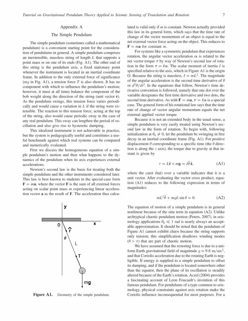
The simple pendulum (sometimes called a mathematicalpendulum) is a convenient starting point for the considera-tion of pendulums in general. A simple pendulum comprisesan inextensible, massless string of length L that supports apoint mass m on one of its ends (Fig. A1). The other end ofthis string is the pendulum axis, a fixed stationary pointwhenever the instrument is located in an inertial coordinateframe. In addition to the only external force of significance(mg in Fig. A1), a tension force T is also shown. It has nocomponent with which to influence the pendulum’s motion;however, it must at all times balance the component of thebob weight along the direction of the string (unit vector r).As the pendulum swings, this tension force varies periodi-cally and would cause a variation in L if the string were ex-tensible. The reaction to this tension force, acting at the topof the string, also would cause periodic sway in the case ofany real pendulum. This sway can lengthen the period of os-cillation and also give rise to hysteretic damping.

This idealized instrument is not achievable in practice,but the system is pedagogically useful and constitutes a use-ful benchmark against which real systems can be comparedand numerically evaluated.

First we discuss the homogeneous equation of a sim-ple pendulum’s motion and then what happens to the dy-namics of the pendulum when its axis experiences externalaccelerations.

Newton’s second law is the basis for treating both thesimple pendulum and the other instruments considered later.This law is best known to students in the special-case formF � ma, where the vector F is the sum of all external forcesacting on scalar point mass m experiencing linear accelera-tion vector a as the result of F. The acceleration thus calcu-

lated is valid only if m is constant. Newton actually providedthis law in its general form, which says that the time rate ofchange of the vector momentum of an object is equal to thenet external vector force acting on the object. This reduces toF � ma for constant m.

For systems like a symmetric pendulum that experiencesrotation, the angular vector acceleration α is related to thenet vector torque τ by way of Newton’s second law of rota-tion in the form τ � Iα. The scalar moment of inertia I isspecified relative to the axis, which in Figure A1 is the originO. Because the string is massless, I � mL2. The magnitudeof the angular acceleration is the second time derivative of θor d2θ=dt2. In the equations that follow, Newton’s time de-rivative convention is followed, namely that one dot over thevariable designates the first time derivative and two dots, thesecond time derivative. As with F � ma, τ � Iα is a specialcase. The general form of his rotational law says that the timerate of change of vector angular momentum equals the netexternal applied vector torque.

Because it is not an extended body in the usual sense, asimple pendulum is very easily treated using Newton’s sec-ond law in the form of rotation. To begin with, followinginitialization at θ0 ≠ 0, let the pendulum be swinging in freedecay in an inertial coordinate frame (Fig. A1). For positivedisplacement θ corresponding to a specific time (the θ direc-tion is along the z axis), the torque due to gravity at that in-stant is given by

τ � Lr ×mg � I�θ z; (A1)

where the caret (hat) over a variable indicates that it is aunit vector. After evaluating the vector cross product, equa-tion (A1) reduces to the following expression in terms ofmagnitudes:

mL2 �θ�mgL sin θ � 0: (A2)

The equation of motion of a simple pendulum is in generalnonlinear because of the sine term in equation (A2). Unlikearchtypical chaotic pendulum motion (Peters, 2007), in seis-mology applications θ0 ≪ 1 rad is nearly always an accept-able approximation. It should be noted that the pendulum ofFigure A1 cannot exhibit chaos because the string supportsonly tension; this simplification disallows winding modes(θ > π) that are part of chaotic motion.

We have assumed that the restoring force is due to a uni-form Earth gravitational field of magnitude g≈ 9:8 m=sec2,and that Coriolis acceleration due to the rotating Earth is neg-ligible. If energy is supplied to a simple pendulum to offsetits damping, and if the pendulum is located somewhere otherthan the equator, then the plane of its oscillation is steadilyaltered because of the Earth’s rotation. Aczel (2004) providesa fascinating account of Leon Foucault’s invention of thisfamous pendulum. For pendulums of a type common to seis-mology, physical constraints against axis rotation make theCoriolis influence inconsequential for most purposes. For aFigure A1. Geometry of the simple pendulum.

Tutorial on Gravitational Pendulum Theory Applied to Seismic Sensing of Translation and Rotation 7

pendulum whose effective length is an appreciable fractionof the Earth radius, such as the Schuler pendulum (Akiand Richards, 2002), the uniform-field approximation isnot valid.

Although not shown in Figure A1, further assume thatthe only other external force acting on the pendulum is oneof frictional retardation, viscous damping. With all theseapproximations, the equation of motion for the nondrivensimple pendulum takes on the simple linear form

�θ� ωo

Q_θ� ω2

oθ � 0; ω2o � g

L: (A3)

This simple-harmonic-oscillator-with-viscous-dampingequation is the heart of linear-approximate models of thependulum and many other mechanical oscillators. It is ap-plicable to the pendulum only to the extent that sin θ≈ θis acceptable and also that its loss of oscillatory energyderives from damping friction that is proportional to the firstpower of the velocity. With damping included in the equationof motion

τ � �Lc_θ �mgL sin θ � mL2 �θ; (A4)

where c_θ is the viscous friction force, assumed proportionalto the angular velocity through the coefficient c, acting on thebob of mass m at a distance L from the axis. It should benoted that c is not always constant (Peters, 2004).

The adjective “mathematical” is appropriate to describea simple pendulum because real instruments are never assimple as the assumptions made concerning its structure.In addition, a damping term proportional to the velocity doesnot fully describe the behavior of real oscillators.

The first person to introduce viscous damping to thesimple harmonic oscillator may have been physicist HendrikAnton Lorentz (1853–1928). Neither Lorentz nor GeorgeGabriel Stokes (1819–1903) treated the viscous model asloosely as has been common in recent years (Peters, 2005a).

The quality factor is defined by Q � �2πE=ΔE, whereE is the energy of oscillation and ΔE is the energy lost percycle due to the damping. One can easily estimate Q to a fewpercent from an exponential free decay as follows. After ini-tializing the motion at a given amplitude, count the numberof oscillations required for the amplitude to decay to 1=e≈0:368 of the initial value. Q is then obtained by multiplyingthis number by π.

For linear viscous damping, a simple relationship existsbetween Q and the damping (decay) coefficient β, used withthe exponential to describe the turning points of the motionthrough exp��βt�:

Q � ωo

2β� ωo

mL

c: (A5)

It should be noted that if β were a constant, then Q would beproportional to the natural frequency f0 through ω0 � 2πf0.As demonstrated by Streckeisen, circa 1960, (E. Wielandt,

personal comm., 2000) with a LaCoste-spring vertical seis-mometer, the Q of practical instruments is not proportionalto f0. At least for instruments configured to operate with along-natural period, the proportionality is one involving f20.For these systems, the damping derives from internal frictionin spring and pivot materials, and the best simple model isnonlinear (Peters, 2005a). Although it involves the velocityonly by way of algebraic sign, this form of damping is non-linear, even so resulting in exponential free decay. Althoughthe coefficient β may be reasonably called a damping coeffi-cient, it is not proper to call it a damping constant, because itis not constant but varies with frequency.

Swinging in a fluid such as air, a real pendulum experi-ences two drag forces, one acting on the bob and the otheracting on the string. This problem was first treated analyti-cally by Stokes (1850), originator of the drag-force law f �6πηRv for a small sphere of radius R falling in a liquid atterminal velocity v in a fluid of viscosity η. However, thisequation does not in general allow an accurate theoreticalestimate of Q based simply on the fluid’s viscosity. Stokes’law can be used only when working with very small parti-cles. In particular, for a macroscopic pendulum,the Reynoldsnumber is generally too large to allow its use. In most casesthe air influence must include a quadratic velocity term aswell as the linear term assumed for equation (A3) (Nelsonand Olsson, 1986). In other words, even air damping is notnecessarily linear.

In the case of extended rigid bodies undergoing periodicflexure during oscillation, several damping mechanisms gen-erally are present. Internal friction in pivot and structure usu-ally contributes significantly, sometimes dominantly (Peters,2004). The net quality factor describing the decay is given by

1

QNet� 1

Q1

� 1

Q2

� � � � ; (A6)

where it is seen that the damping mechanism with the low-est quality factor dominates. Only for those mechanismsthat give rise to exponential decay is Q independent ofthe pendulum’s amplitude. With quadratic-in-velocity fluiddamping, the amplitude trend of Q is opposite to that ofCoulomb friction. Unlike hysteretic and viscous damping,neither of these nonlinear mechanisms yields an exponentialfree decay.

The subscript zero used with ω in equation (A3) is anatural consequence of the mathematical solution to the dif-ferential equation. A subscript corresponding to the eigen-frequency of the pendulum in the absence of damping(Q → ∞) is used to distinguish this value from the red-shifted frequency when there is damping; that is, ω ��ω2

0 � β2�1=2. This redshift is negligible except, perhapswhere the pendulum damping is near critical (Q≈ 0:5).When internal-friction hysteretic damping is the dominantsource of damping, the redshift has no meaning becausethere is no mechanism to cause it (Peters, 2005a).

8 R. D. Peters

Fortunately, when seismic instruments are operated withnear-critical damping (Q � 1=

���2

p), the assumption of linear

viscous damping is for many purposes adequate. Such is thecase, for example, when eddy-current damping is employed.It is also true for damping provided by force-balance feed-back. In general, however, the damping of an instrument isnot governed by a linear equation of motion.

The Driven Simple Pendulum

When the axis of the pendulum undergoes accelera-tion a�t�, application of Newton’s laws shows that the zeroon the right-hand side of equation (A3) simply is replacedby �ω2

0a�t�=g. Conceptual understanding of this term isstraightforward. Given that the effect of acceleration a andgravitational field g are indistinguishable to the pendulum(it measures acceleration at one location only) and that atequilibrium in the absence of a the string is oriented alongthe direction of the acceleration vector g from the Earth’sgravity, then when there is a constant acceleration a of thecase perpendicular to g the string now aligns itself with thevector sum g � a. If g could be set to zero, alignment wouldbe with�a. Thus, the magnitude of the pendulum deflectionangle (for a ≪ g) is given by θ � a=g. The same result ap-plies for a harmonic acceleration whose frequency is signifi-cantly less than the natural frequency of the pendulum. Forsuch an excitation, the derivative terms in the left-hand sideof the equation of motion are negligible. In turn it is recog-nized that �a=g must be multiplied by ω2

0 to obtain the right-hand side of the now inhomogeneous equation.

Using complex exponentials to describe the steady-stateresponse to harmonic excitation (a pendulum entrained withthe drive after transients have settled) yields

���� gθ0a0;ground

����� ω20���������������������������������������������

�ω20 � ω2�2 � ω2

0ω2=Q

p ; (A7)

where a0;ground is the amplitude of the pivot’s accelerationa�t� and is responsible for the angular displacement ampli-tude of the pendulum θ0. We refer to equation (A7) as themagnitude of the acceleration transfer function of the sim-ple pendulum, expressed in terms of angular displacement.Other transfer function forms are also considered in thisarticle. Such functions are always a complex steady-state di-mensionless ratio. Although axis (pivot) acceleration is thestate variable responsible for exciting the pendulum, it is pos-sible to define transfer functions in terms of the other statevariables.

I next examine the ratio of the displacement of the pen-dulum bob to the displacement of the accelerating ground.Because this ratio is complex, it has both a magnitudeand a phase. Alternatively, this transfer function could be de-scribed in terms of its real and imaginary components thoughthis is rarely done in seismology.

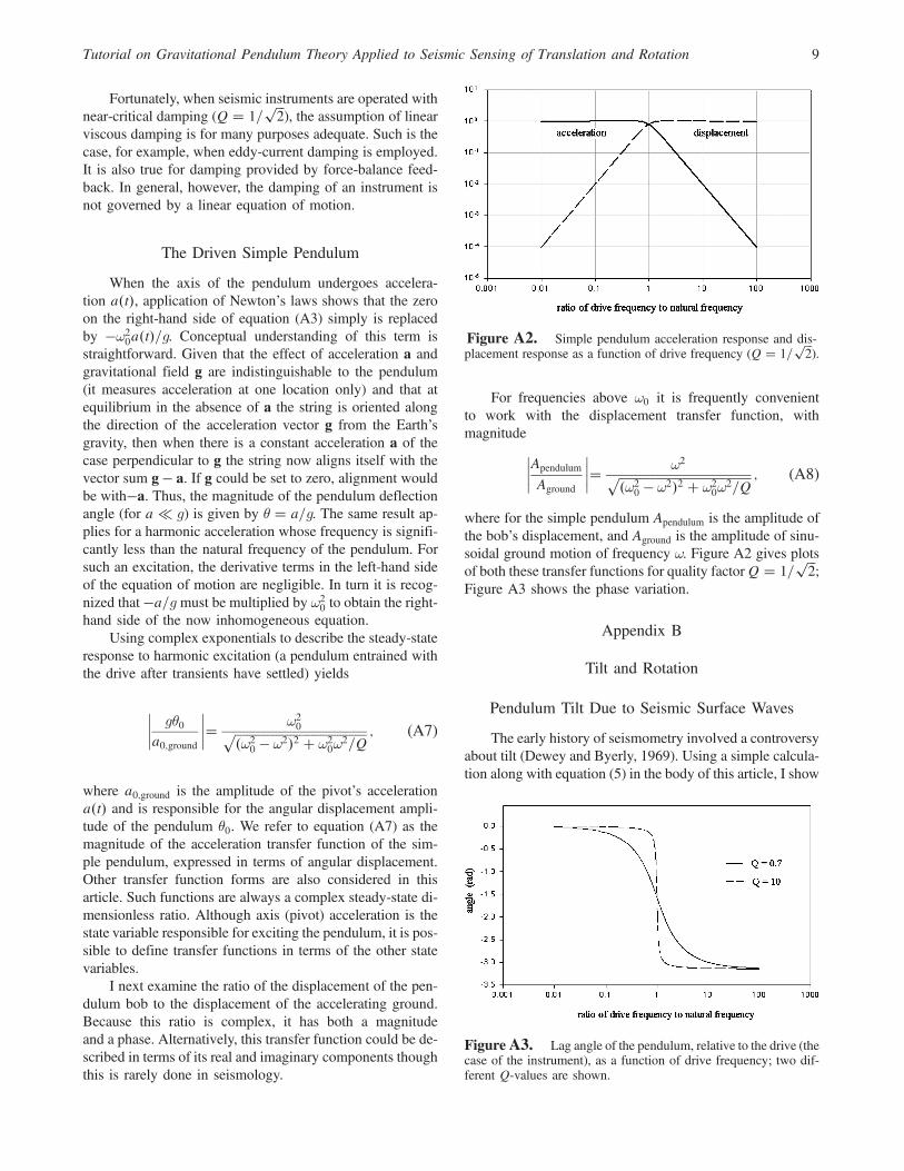
For frequencies above ω0 it is frequently convenientto work with the displacement transfer function, withmagnitude

����Apendulum

Aground

����� ω2����������������������������������������������ω2

0 � ω2�2 � ω20ω

2=Qp ; (A8)

where for the simple pendulum Apendulum is the amplitude ofthe bob’s displacement, and Aground is the amplitude of sinu-soidal ground motion of frequency ω. Figure A2 gives plotsof both these transfer functions for quality factorQ � 1=

���2

p;

Figure A3 shows the phase variation.

Appendix B

Tilt and Rotation

Pendulum Tilt Due to Seismic Surface Waves

The early history of seismometry involved a controversyabout tilt (Dewey and Byerly, 1969). Using a simple calcula-tion along with equation (5) in the body of this article, I show

Figure A2. Simple pendulum acceleration response and dis-placement response as a function of drive frequency (Q � 1=

���2

p).

Figure A3. Lag angle of the pendulum, relative to the drive (thecase of the instrument), as a function of drive frequency; two dif-ferent Q-values are shown.

Tutorial on Gravitational Pendulum Theory Applied to Seismic Sensing of Translation and Rotation 9

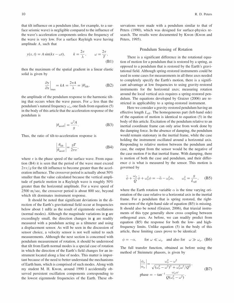
that tilt influence on a pendulum (due, for example, to a sur-face seismic wave) is negligible compared to the influence ofthe wave’s acceleration components unless the frequency ofthe wave is very low. For a surface Rayleigh wave havingamplitude A, such that

y�x; t� � A sin�kx � ωt�; k � 2πλ; ω � 2π

T;

(B1)

then the maximum of the spatial gradient in a linear elasticsolid is given by

∂y∂x

����max

� kA � 2πAλ

� jθjtilt; (B2)

the amplitude of the pendulum response to the harmonic tilt-ing that occurs when the wave passes. For ω less than thependulum’s natural frequency ωo, one finds from equation (5)in the body of this article that the acceleration response of thependulum is

jθaccelj �ω2A

g: (B3)

Thus, the ratio of tilt-to-acceleration response is

���� θtiltθaccel

����� gT

2πv; (B4)

where v is the phase speed of the surface wave. From equa-tion (B4) it is seen that the period of the wave must exceed2πv=g for the tilt influence to become greater than the accel-eration influence. The crossover period is actually about 50%smaller than the value calculated because the vertical ampli-tude of particle motion in a Rayleigh wave is roughly 50%greater than the horizontal amplitude. For a wave speed of2500 m=sec, the crossover period is about 800 sec, beyondwhich tilt dominates instrument response.

It should be noted that significant deviations in the di-rection of the Earth’s gravitational field occur at frequenciesbelow about 1 mHz as the result of eigenmode oscillations(normal modes). Although the magnitude variations in g areexceedingly small, the direction changes in g are readilymeasured with a pendulum acting as a tiltmeter and usinga displacement sensor. As will be seen in the discussion ofsensor choice, a velocity sensor is not well suited to suchmeasurements. Although the next section is concerned withpendulum measurement of rotation, it should be understoodthat tilt from Earth normal modes is a special case of rotationin which the direction of the Earth’s field changes for an in-strument located along a line of nodes. This matter is impor-tant because of the need to better understand the mechanismsof Earth hum, which is comprised of such modes. Along withmy student M. H. Kwon, around 1990 I accidentally ob-served persistent oscillation components corresponding tothe lowest eigenmode frequencies of the Earth. These ob-

servations were made with a pendulum similar to that ofPeters (1990), which was designed for surface-physics re-search. The results were documented by Kwon (Kwon andPeters, 1995).

Pendulum Sensing of Rotation

There is a significant difference in the rotational equa-tion of motion for a pendulum that is restored by a spring, asopposed to a pendulum that is restored by the Earth’s gravi-tational field. Although spring-restored instruments could beused in some cases for measurements in all three axes neededto completely specify the Earth's motion, there is a signifi-cant advantage at low frequencies to using gravity-restoredinstruments for the horizontal axes; measuring rotationaround the local vertical axis requires a spring-restored pen-dulum. The equations developed by Graizer (2006) are re-stricted in applicability to a spring-restored instrument.

Here we consider a gravity-restored pendulum having aneffective length Leff . The homogeneous part (left-hand side)of the equation of motion is identical to equation (5) in thebody of this article. Excitation of the pendulum relative to aninertial coordinate frame can only arise from work done bythe damping force. In the absence of damping, the pendulumwould remain stationary in the inertial frame, while the caseholding the instrument oscillated around a horizontal axis.Responding to relative motion between the pendulum andcase, the output from the sensor would be the negative ofthe case motion θ in that inertial frame. With damping, thereis motion of both the case and pendulum, and their differ-ence ϕ is what is measured by the sensor. This motion isgoverned by

�ϕ� ωo

Q_ϕ� ω2

oϕ � � �α � ω2oα; ω2

o � g

Leff; (B5)

where the Earth rotation variable α is the time varying ori-entation of the case relative to a horizontal axis in the inertialframe. For a pendulum that is spring restored, the right-most term of the right-hand side of equation (B5) is missing.It should also be noted (Graizer, 2006), that triaxial instru-ments of this type generally show cross coupling betweenorthogonal axes. As before, we can readily predict fromequation (B5) the response for both the low- and high-frequency limits. Unlike equation (5) in the body of thisarticle, these limiting cases prove to be identical:

ϕ � �α; for ω ≪ ωo and also for ω ≫ ωo: (B6)

The full transfer function, obtained as before using themethod of Steinmetz phasors, is given by

����ϕo

αo

����� ω2o � ω2������������������������������������������������

�ω2o � ω2�2 � ω2

oω2=Q2p ;

phase � � tan�1ωoω

Q�ω2o � ω2� :

(B7)

10 R. D. Peters

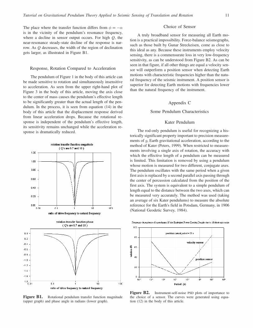
The place where the transfer function differs from ϕ � �αis in the vicinity of the pendulum’s resonance frequency,where a decline in sensor output occurs. For high Q, thenear-resonance steady-state decline of the response is nar-row. As Q decreases, the width of the region of declinationgets larger, as illustrated in Figure B1.

Response, Rotation Compared to Acceleration

The pendulum of Figure 1 in the body of this article canbe made sensitive to rotation and simultaneously insensitiveto acceleration. As seen from the upper right-hand plot ofFigure 3 in the body of this article, moving the axis closeto the center of mass causes the pendulum’s effective lengthto be significantly greater than the actual length of the pen-dulum. In the process, it is seen from equation (14) in thebody of this article that the displacement response derivedfrom linear acceleration drops. Because the rotational re-sponse is independent of the pendulum’s effective length,its sensitivity remains unchanged while the acceleration re-sponse is dramatically reduced.

Choice of Sensor

A truly broadband sensor for measuring all Earth mo-tion is a practical impossibility. Force-balance seismographs,such as those built by Gunar Streckeisen, come as close tothis ideal as any. Because these instruments employ velocitysensing, there is a commensurate loss in very low-frequencysensitivity, as can be understood from Figure B2. As can beseen in that figure, if all other things are equal a velocity sen-sor will outperform a position sensor when detecting Earthmotions with characteristic frequencies higher than the natu-ral frequency of the seismic instrument. A position sensor issuperior for detecting Earth motions with frequencies lowerthan the natural frequency of the instrument.

Appendix C

Some Pendulum Characteristics

Kater Pendulum

The rod-only pendulum is useful for recognizing a his-torically significant property important to precision measure-ments of g, Earth gravitational acceleration, according to themethod of Kater (Peters, 1999). When restricted to measure-ments involving a single axis of rotation, the accuracy withwhich the effective length of a pendulum can be measuredis limited. This limitation is removed by using a pendulumwhose motion is measured for two different, conjugate axes.The pendulum oscillates with the same period when a givenfirst axis is replaced by a second parallel axis passing throughthe center of percussion calculated from the position of thefirst axis. The system is equivalent to a simple pendulum oflength equal to the distance between the two axes, which canbe measured very accurately. The method was used (takingan average of six Kater pendulums) to measure the absolutereference for the Earth's field in Potsdam, Germany, in 1906(National Geodetic Survey, 1984).

Figure B1. Rotational pendulum transfer function magnitude(upper graph) and phase angle in radians (lower graph).

Figure B2. Instrument-self-noise PSD plots of importance tothe choice of a sensor. The curves were generated using equa-tion (12) in the body of this article.

Tutorial on Gravitational Pendulum Theory Applied to Seismic Sensing of Translation and Rotation 11

Advantages of a Pendulum with M1 ≠ 0

Compared to a pendulum of the type shown in Figure 1in the body of this article, where much of the total mass isconcentrated in the dense upper component, M1, the me-chanical integrity of a rod-only pendulum is significantlylower. To obtain the long periods needed for rotationalsensing, the axis must be positioned close to the center ofthe rod. The portion above the axis that results, almostL=2 in length, is subject to considerable creep deformation(Peters, 2005b).

Of course the other disadvantage of the rod-only config-uration involves the greater size of the instrument. Reducingthe height by means of a concentrated upper mass allows asmaller size and reduced cost for the instrument’s case. Ad-ditionally, the smaller case reduces air-current disturbancesdue to convective circulation.

Frequency Dependence of Sensitivity

The response of a pendulum is quite different whenthe drive acceleration at the axis is at an angular frequencysignificantly lower than or higher than the eigenfrequency.The extremes of these two cases are readily treated by avisual inspection of the equation of motion. From equa-tion (5) in the body of this article we can readily deducethe following:

Low-Frequency Sensitivity Limit

When the drive frequency is very low, the first and sec-ond time derivatives of θ are insignificant compared to theremaining term. Thus,

θ � � aaxisg

; ω ≪ ωo: (C1)

It is important to understand from equation (C1) that the pen-dulum’s angular sensitivity to acceleration at frequencieswell below its natural frequency is independent of the posi-tion of the axis. equation (C1) is a general result, no matterthe pendulum type. Typically, however, we do not employ asensor that measures θ directly but rather a detector is placedat the bottom end of the pendulum where it measures thetransverse displacement relative to the instrument’s case.The amount of motion at the bottom scales with length L,which scales (for a simple pendulum) with the square ofthe instrument’s natural period. Thus, we see that sensitiv-ity to acceleration is proportional to the square of this natu-ral period. To maximize the low-frequency sensitivity of anopen-loop (i.e., nonfeedback) system, one should operatewith as long a natural period as is conveniently possible, thusthe very long natural periods of modern broadband velocityseismometers.

High-Frequency Sensitivity Limit

When the drive frequency is very high, the second de-rivative term in equation (5) in the body of the article is sig-nificantly greater than the other terms on the left-hand sideof the equation. Additionally (once transients have decayedaway) the pendulum is entrained with the drive and differs inphase by 180°. Entrainment means that the only frequency ofpendulum motion is the frequency of the drive. Prior to en-trainment, during the transient, both the natural frequency ofthe pendulum and the frequency of the drive are simulta-neously present. Thus, its steady-state frequency is the sameas that of a�t�, namely ω. Assuming monochromatic simpleharmonic motion, we obtain

θo � �ω2o

gAground; (C2)

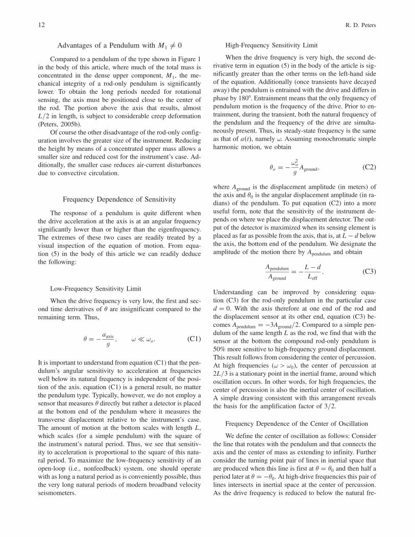
where Aground is the displacement amplitude (in meters) ofthe axis and θ0 is the angular displacement amplitude (in ra-dians) of the pendulum. To put equation (C2) into a moreuseful form, note that the sensitivity of the instrument de-pends on where we place the displacement detector. The out-put of the detector is maximized when its sensing element isplaced as far as possible from the axis, that is, at L � d belowthe axis, the bottom end of the pendulum. We designate theamplitude of the motion there by Apendulum and obtain

Apendulum

Aground� �L � d

Leff: (C3)

Understanding can be improved by considering equa-tion (C3) for the rod-only pendulum in the particular cased � 0. With the axis therefore at one end of the rod andthe displacement sensor at its other end, equation (C3) be-comes Apendulum � �3Aground=2. Compared to a simple pen-dulum of the same length L as the rod, we find that with thesensor at the bottom the compound rod-only pendulum is50% more sensitive to high-frequency ground displacement.This result follows from considering the center of percussion.At high frequencies (ω > ω0), the center of percussion at2L=3 is a stationary point in the inertial frame, around whichoscillation occurs. In other words, for high frequencies, thecenter of percussion is also the inertial center of oscillation.A simple drawing consistent with this arrangement revealsthe basis for the amplification factor of 3=2.

Frequency Dependence of the Center of Oscillation

We define the center of oscillation as follows: Considerthe line that rotates with the pendulum and that connects theaxis and the center of mass as extending to infinity. Furtherconsider the turning point pair of lines in inertial space thatare produced when this line is first at θ � θ0 and then half aperiod later at θ � �θ0. At high-drive frequencies this pair oflines intersects in inertial space at the center of percussion.As the drive frequency is reduced to below the natural fre-

12 R. D. Peters

quency of the pendulum, the intersection of this line-pairmoves downward.

The term percussion implies a short lived impulse; as thedriving period lengthens, the percussion point is no longer ameaningful reference for the inertial center of rotational mo-tion. The center of oscillation remains meaningful but is nolonger located at the center of percussion. As the drive fre-quency goes toward zero, the center of oscillation moves to-ward infinity. A (false) assumption that some part of theinertial mass of a seismometer remains stationary in spaceas the instrument case moves is acceptable when the instru-ment is functioning as a vibrometer (i.e., drive frequenciesabove the natural frequency), but it is not true for the low-frequency extreme of the pendulum’s response.

Appendix D

Unconventional and Exotic Pendulums

Unconventional Pendulums

Rotation Sensor

Two very different, unconventional gravitational com-pound pendulums are described in this appendix. Illustratedin Figure D1 is a rotation sensor capable of operating over abroad frequency range. Whereas the pendulum of Figure 1in the body of this article is a rigid vertical-at-equilibriumstructure that oscillates about a horizontal axis, the rigidbeam of the pendulum illustrated in Figure D1 is horizontal-at-equilibrium. I believe there are three advantages to thissystem, although they have not all been experimentally veri-fied. First, the influence of creep is expected to be less for thehorizontal configuration as compared to the vertical one.Creep in the members of the long-period vertical pendulumalters the equilibrium position, whereas creep of the boom inthe horizontal pendulum alters the period. Secular change inthe equilibrium position decreases the maximum possiblesensitivity of an instrument’s detector, unless force feedbackis employed. Period change is inconsequential except as itincreases responsiveness to translational acceleration. Be-cause the instrument is designed to minimize this response,the creep influence is of secondary rather than primary im-portance as in the case of the vertical pendulum.

The second advantage involves air currents. A thermalgradient within the container that holds the instrument can

cause convective flows, and the resulting circulation is ex-pected to have greater influence on the vertical pendulumthan on the horizontal pendulum.

The final advantage results from the simple means bywhich one mounts a pair of displacement detectors on oppo-site ends of the beam. Operating differentially in phase op-position, they yield a better signal-to-noise ratio (SNR) thanis possible from a single detector. The greater the length ofthe beam, the greater will be the sensitivity of the instrument.

Some Other Inertial Rotation Sensors

Parts from a pair of STS-1 horizontal seismometers wereused to build a rotation sensor with mechanical propertiessimilar to the rotation pendulums I have described. The in-strument tested by Hutt et al. (2004) differs, however, bycontaining springs; the lower flexures are placed under ten-sion by means of a large brass counterweight.

Morrissey (2000) also built a beam-balance broadbandtiltmeter with similar mechanical properties. His instrumentused a pair of lead masses mounted on opposite ends of ahorizontal aluminum bar suspended at the center with aflexural axis. It used force-feedback balancing and heclaimed a sensitivity of 120 mV=μrad, with a resolutionof better than 0.1 nrad, using linear variable differential trans-formers (LVDT). Wielandt (2002) notes that a capacitive sen-sor is superior to an LVDT for the reason of the granularnature of ferromagnetism of the latter. Compared to a capac-itive sensor of (singly) differential type which is customary,there is an SNR advantage to using a pair of (doubly � fully)differential capacitive sensors with the pendulum of Fig-ure D1, one such fully-differential detector for each end, withthe pair operating in phase opposition.

Microseism Detector

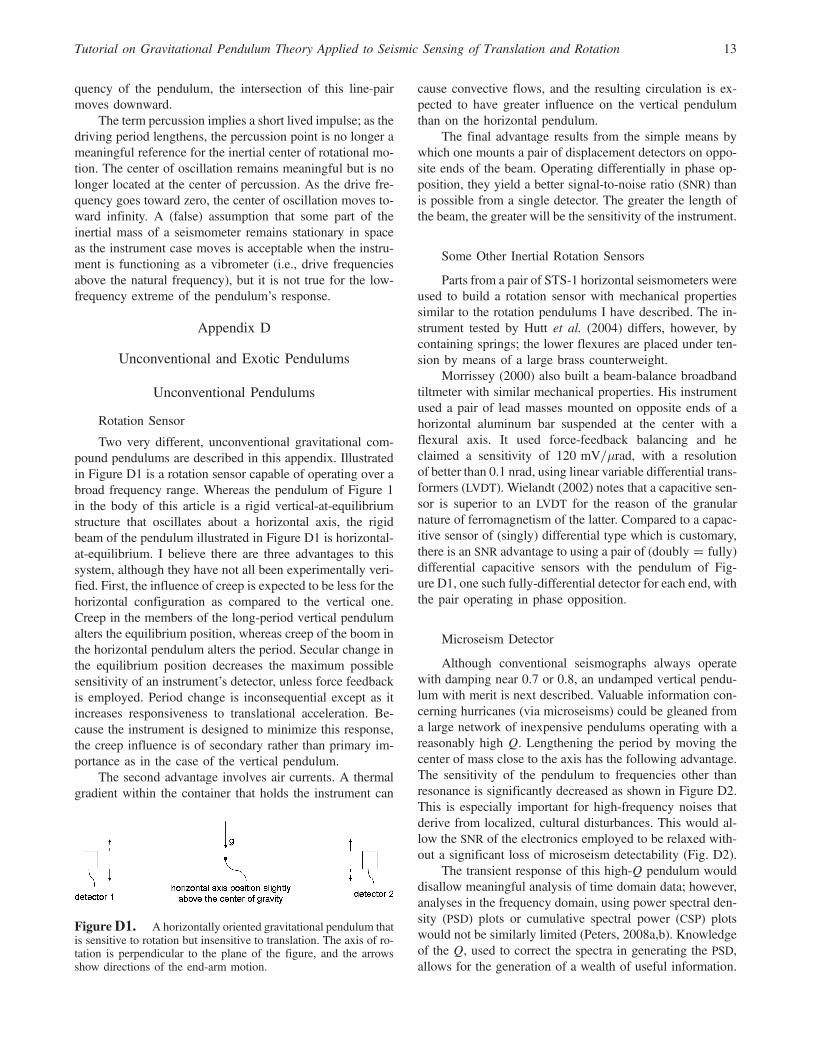
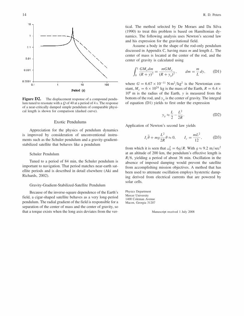
Although conventional seismographs always operatewith damping near 0.7 or 0.8, an undamped vertical pendu-lum with merit is next described. Valuable information con-cerning hurricanes (via microseisms) could be gleaned froma large network of inexpensive pendulums operating with areasonably high Q. Lengthening the period by moving thecenter of mass close to the axis has the following advantage.The sensitivity of the pendulum to frequencies other thanresonance is significantly decreased as shown in Figure D2.This is especially important for high-frequency noises thatderive from localized, cultural disturbances. This would al-low the SNR of the electronics employed to be relaxed with-out a significant loss of microseism detectability (Fig. D2).

The transient response of this high-Q pendulum woulddisallow meaningful analysis of time domain data; however,analyses in the frequency domain, using power spectral den-sity (PSD) plots or cumulative spectral power (CSP) plotswould not be similarly limited (Peters, 2008a,b). Knowledgeof the Q, used to correct the spectra in generating the PSD,allows for the generation of a wealth of useful information.

Figure D1. A horizontally oriented gravitational pendulum thatis sensitive to rotation but insensitive to translation. The axis of ro-tation is perpendicular to the plane of the figure, and the arrowsshow directions of the end-arm motion.

Tutorial on Gravitational Pendulum Theory Applied to Seismic Sensing of Translation and Rotation 13

Exotic Pendulums

Appreciation for the physics of pendulum dynamicsis improved by consideration of unconventional instru-ments such as the Schuler pendulum and a gravity-gradient-stabilized satellite that behaves like a pendulum

Schuler Pendulum

Tuned to a period of 84 min, the Schuler pendulum isimportant to navigation. That period matches near-earth sat-ellite periods and is described in detail elsewhere (Aki andRichards, 2002).

Gravity-Gradient-Stabilized-Satellite Pendulum

Because of the inverse-square dependence of the Earth’sfield, a cigar-shaped satellite behaves as a very long-periodpendulum. The radial gradient of the field is responsible for aseparation of the center of mass and the center of gravity, sothat a torque exists when the long axis deviates from the ver-

tical. The method selected by De Moraes and Da Silva(1990) to treat this problem is based on Hamiltonian dy-namics. The following analysis uses Newton’s second lawand his expression for the gravitational field.

Assume a body in the shape of the rod-only pendulumdiscussed in Appendix C, having mass m and length L. Thecenter of mass is located at the center of the rod, and thecenter of gravity is calculated using

ZL

0

GMedm

�R� y�2 �mGMe

�R� yg�2; dm � m

Ldy; (D1)

where G � 6:67 × 10�11 Nm2=kg2 is the Newtonian con-stant, Me � 6 × 1024 kg is the mass of the Earth, R � 6:4 ×106 m is the radius of the Earth, y is measured from thebottom of the rod, and yg is the center of gravity. The integralof equation (D1) yields to first order the expression

yg ≈ L

2� L2

2R: (D2)

Application of Newton’s second law yields

Ic �θ�mgL2

2Rθ≈ 0; Ic �

mL2

12; (D3)

from which it is seen that ω20 � 6g=R. With g≈ 9:2 m=sec2

at an altitude of 200 km, the pendulum’s effective length isR=6, yielding a period of about 36 min. Oscillation in theabsence of imposed damping would prevent the satellitefrom accomplishing mission objectives. A method that hasbeen used to attenuate oscillation employs hysteretic damp-ing derived from electrical currents that are powered bysolar cells.

Physics DepartmentMercer University1400 Coleman AvenueMacon, Georgia 31207

Manuscript received 1 July 2008

Figure D2. The displacement response of a compound pendu-lum tuned to resonate with aQ of 40 at a period of 4 s. The responseof a near-critically damped simple pendulum of comparable physi-cal length is shown for comparison (dashed curve).

14 R. D. Peters