Tutorial on DFPT and TD-DFPT:calculations of phonons and

absorption spectra

Iurii Timrov

SISSA – Scuola Internazionale Superiore di Studi Avanzati, Trieste – Italy

itimrov@sissa.it

Computer modelling of materials at the nanoscaleThe University of Tokyo, Japan

25 April 2014

Outline

This afternoon

Density functional perturbation theory (DFPT)

Time-dependent density functional perturbation theory (TDDFPT)

● Introduction

● Exercise 1: Phonon calculations at Γ

● Exercise 2: Phonon dispersion

● Introduction

● Exercise 1: Calculation of independent particle spectrum

● Exercise 2: turboDavidson

● Exercise 3: turboLanczos

Part 1 : Calculation of phonons

Let us consider a unit cell with atoms.

Phonons

is the point in the Bravais-lattice, identifying the position of a given unit cell

is the -component of the displacement of s-th atom

variables

Interatomic Force Constants :

is the number of unit cells in the crystal

index of an atom in the unit cell

is the Cartesian index

PhononsFourier transformation:

Essence of the Bloch theorem:

Important concept: We can perform calculations of Interatomic Force Constants for each q independently !!!

Phonons

Sampling theoremThe number of q points is equal to the number of R points at which Interatomic Force Constants are computed.

Important concept: Instead of Interatomic Force Constants we need only !!!

Phonons

Normal mode frequencies, , and eigenvectors, are determined by the secular equation:

where

is the dynamical matrix.

Diagonalization of dynamical matrix gives phonon modes at q.

Interatomic Force Constants (IFC)

Exercise 1: Phonon calculations at Γ

Go to the directory with the input files:

cd Part1_phonons/exercise1

In this directory you will find:

● README – File describing how to do the exercise

● Si.scf.in – Input file for the SCF calculation

● Si.ph.in – Input file for the phonon calculation at Γ

● Si.vbc.UPF – Pseudopotential of silicon

● reference – Directory with the reference results

● out – Directory for temporary files

Exercise 1: Phonon calculations at ΓStep 1. Perform an SCF calculation for silicon at the equilibrium structure using the code pw.x

Exercise 1: Phonon calculations at Γ

Step 2. Perform a phonon calculation at Γ using the code ph.x

The same prefix as in the SCF calculation Threshold for self-consistencyAtomic massDirectory for temporary filesFile containing the dynamical matrix

Coordinates of the q point in units of 2*pi/a in Cartesian framework

Exercise 1: Phonon calculations at ΓDynamical matrix file Si.dyn :

Exercise 1: Phonon calculations at Γ

Acoustic sum rule at Γ

Because of numerical inaccuracies the interatomic force constants do not strictly satisfy the acoustic sum rule (ASR).

However, the ASR can be imposed using the code dynmat.x .

The input is Si.dynmat.in :

File containing the dynamical matrix

A way to impose the acoustic sum rule

Exercise 1: Phonon calculations at Γ

The program dynmat.x produces the file dynmat.out which contains the new frequencies:

Exercise 2: Phonon dispersionGo to the directory with the input files:

cd Part1_phonons/exercise2

In this directory you will find:

● README – File describing how to do the exercise

● Si.scf.in – Input file for the SCF calculation

● Si.ph.in – Input file for the phonon calculation on a q-grid

● Si.q2r.in – Input file for calculation of Interatomic Force Constants

● Si.matdyn.in – Input file for Fourier Interpolation for various q points

● Si.plotband.in – Input file for plotting a phonon dispersion

● Si.vbc.UPF – Pseudopotential of silicon

● reference – Directory with the reference results

● out – Directory for temporary files

Exercise 2: Phonon dispersion

Step 1. Perform an SCF calculation for silicon at the equilibrium structure using the code pw.x

Step 2. Perform a phonon calculation on a uniform grid of q points using the code ph.x

Option for the calculation on a grid

Uniform grid of q points

Exercise 2: Phonon dispersion

● The phonon code ph.x generates the files of the dynamical matrices on the specified grid of q points. The files are Si.dyn1, Si.dyn2, ..., Si.dyn8.

● The file Si.dyn0 contains the list of the inequivalent q points (8, in this case).

Exercise 2: Phonon dispersion

Step 3. Calculation of the Interatomic Force Constants (IFC) using the code q2r.x

are Cartesian components, and are atomic indices.

Fourier transforms of IFC's on a gridof q points nq1 x nq2 x nq3in reciprocal space

IFC's in a supercell nq1 x nq2 x nq3in real space

Fourier transforms of IFC's :

Exercise 2: Phonon dispersion

Input file Si.q2r.in :

Dynamical matrices from the phonon calculationA way to impose the acoustic sum rule

Output file of the interatomic force constants

To perform the calculation:

The denser the grid of q points, the larger the vectors R for which the Interatomic Force Constants are calculated!

Exercise 2: Phonon dispersionStep 4. Calculate phonons at generic q' points using IFC by means of the code matdyn.x

IFC's on a grid in real space Fourier transforms of IFC's at generic q' point in reciprocal space

Fourier interpolation

Input file Si.matdyn.in :

Acoustic sum rule

File with IFC's Atomic mass Atomic mass

Output file with the frequenciesNumber of q pointsNumber of q pointsCoordinates of q points

Exercise 2: Phonon dispersionStep 5. Plot the phonon dispersion using the code plotband.x and gnuplot.

Input file Si.plotband.in :

Input file with the frequencies at various q'

Range of frequencies for a visualizationOutput file with frequencies which will be used for plotPlot of the dispersion (we will produce another one)Fermi level (needed only for band structure plot)

Use gnuplot and the file plot_dispersion.gnu in order to plot the phonon dispersion of silicon (experimental_data.dat). You will obtain a postscript file phonon_dispersion.eps which you can visualize.

Frequency step on the plot freq.psReference frequency on the plot freq.ps

Exercise 2: Phonon dispersionPhonon dispersion of silicon (file phonon_dispersion.eps):

Exercise 2: Phonon dispersionHow to determine whether the quality of the Fourier interpolation is satisfactory? Compare with the direct calculation (no interpolation)!

Exercise 2: Phonon dispersionComparison of the phonon dispersion computed using the Fourier interpolation with the direct calculation at several q points. The q-grid 4x4x4 is very satisfactory for the Fourier interpolation for silicon!

Exercise 2: Phonon dispersionThe agreement of an ab initio calculation of the phonon dispersion using the Fourier interpolation on a q-grid 4x4x4 is excellent with the experimental data!

Exercise 2: Phonon dispersion

The Fourier interpolation works if the Interatomic Force Constants (IFC's) are known on a sufficiently large supercell, i.e. on a large enough grid of q points in the phonon calculation.

There are cases when the IFC's are long range and the Fourier interpolation does not work properly:

● When there are Kohn anomalies in metals. In this case the dynamical matrices are not a smooth function of q and the IFC's are long range.

● In polar insulators where the atomic displacements generate long range electrostatic interactions and the dynamical matrix is not analitical for q→0. However, this case can be dealt with by calculating the Born effective charges and the dielectric tensor of the material.

Part 2 : Calculation of absorption spectra

Independent Particle ApproximationThe simplest approximation: Independet Particle Approximation (IPA) which allows us to describe single-particle excitations.

Fermi's golden rule

The transition probability per unit time from occupied states to empty states reads:

is the external potential induced by the electric field

and are the eigenvalues

are the eigenvalues and the eigenfunctions of the ground-state Kohn-Sham equation

Absorption coefficient:

Exercise 1: Calculation of absorption spectrum of benzene in IPA

Go to the directory with the input files:

cd Part2_absorption_spectra/exercise1

In this directory you will find:

● README – File describing how to do the exercise

● Benzene.scf.in – Input file for the SCF calculation

● Benzene.epsilon.in – Input file for a calculation of spectrum

● H.vbc.UPF – Pseudopotential of hydrogen

● C.vbc.UPF – Pseudopotential of carbon

● plot_spectrum.gnu – Script to plot spectrum using gnuplot

● reference – Directory with the reference results

● out – Directory for temporary files

Exercise 1: Calculation of absorption spectrum of benzene in IPA

Step 1. Perform an SCF calculation for benzene at the equilibrium structure using the code pw.x

Step 2. Perform a calculation of the absorption spectrum for benzene in the independent particle approximation using the code epsilon.x

Exercise 1: Calculation of absorption spectrum of benzene in IPA

Input file for the calculation of spectrum

Type of the calculationThe same prefix as in the SCF calculation Directory for temporary files

Type of smearing of the spectrum The value of the smearing in eVMinimum value of frequencies for a plot in eV Maximum value of frequencies for a plot in eV Number of points between wmin and wmax

The code epsilon.x produces 4 files:

● epsr.dat – Real part of the response

● epsi.dat – Imaginary part of the response (this is what we need)

● eels.dat – Electron energy loss spectrum

● ieps.dat – Response computed on the imaginary axis of frequency

The content of epsi.dat looks like:

Exercise 1: Calculation of absorption spectrum of benzene in IPA

Use gnuplot and the script plot_spectrum.gnu in order to plot the absorption spectrum of benzene Benzene_spectrum.eps

Exercise 1: Calculation of absorption spectrum of benzene in IPA

Absorption spectrum of benzene in the Independent Particle Approximation (file Benzene_spectrum.eps):

turbo-Davidson program for calculation of absorption spectra

● The turbo_davidson.x program allows us to calculate absorption spectra of molecules using linear-response time-dependent density functional theory (TDDFT).

● The interactions of electrons (Hartree and Exchange-Correlation effects) are taken into account fully ab initio and self-consistently.

● The electronic transitions from occupied to empty states can be analyzed by selecting a frequency range in which the transitions are expected to occur.

● However, the overall absorption spectrum in a wide frequency range cannot be calculated at once. Several calculations are required.

Xiao-Chuan Ge's PhD thesis “Seeing colors with TDDFT” http://www.sissa.it/cm/?page_id=85

Linear-response TDDFPT equations:

Rewrite these equations in the matrix form: Casida's equations

turbo-Davidson program for calculation of absorption spectra

where and

interaction term

Davidson algorithm is used (the same algorithm as in the ground state SCF calculation) to solve the Casida's equations and to obtain the eigenvalues which are used for a calculation of the absorption coefficient.

Exercise 2: Calculation of absorption spectrum of benzene using turbo_davidson.x

Go to the directory with the input files:

cd Part2_absorption_spectra/exercise2

In this directory you will find:

● README – File describing how to do the exercise

● Benzene.scf.in – Input file for the SCF calculation

● Benzene.davidson.in – Input file for a Davidson calculation of the eigenvalues

● Benzene.tddfpt_pp.in – Input file for a postprocessing calculation of the spectrum

● H.vbc.UPF – Pseudopotential of hydrogen

● C.vbc.UPF – Pseudopotential of carbon

● plot_spectrum.gnu – Script to plot spectrum using gnuplot

● reference – Directory with the reference results

● out – Directory for temporary files

Exercise 2: Calculation of absorption spectrum of benzene using turbo_davidson.xStep 1. Perform an SCF calculation for benzene at the equilibrium structure using the code pw.x

Step 2. Perform the Davidson calculation without the interaction using the code turbo_davidson.x

The same prefix as in the SCF calculation Directory for temporary files

Switch off the interactionNumber of eigenvalues to be calculatedNumber of initial vectorsMaximum number of basis allowed for the sub-basisConvergence thresholdMinimum value of frequencies for a plot in Ry Maximum value of frequencies for a plot in Ry Frequency step in Ry Lorentzian broadening parameter in Ry Reference frequency in Ry where the peak is expected Number of occupied states to be consideredNumber of empty states to be considered

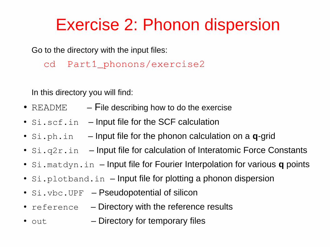
The code turbo_davidson.x produces a file Benzene-dft.eigen :

Exercise 2: Calculation of absorption spectrum of benzene using turbo_davidson.x

Step 3. Perform a spectrum calculation using the postprocessing code turbo_spectrum.x and using the eigenvalues computed in the previous step. The input file Benzene.tddfpt_pp.in reads:

The same prefix as in the SCF calculation Directory for temporary filesType of previous calculationThe value of Lorenzian smearing in RyMinimum value of frequencies for a plot in Ry Maximum value of frequencies for a plot in Ry Frequency step in Ry Frequency with Davidson eigenvalues

Exercise 2: Calculation of absorption spectrum of benzene using turbo_davidson.x

The code turbo_spectrum.x produces a file Benzene.plot which can be

used for plotting the absorption spectrum :

Step 4. Plot the spectrum using gnuplot and the script plot_spectrum.gnu

Since the interaction was switched off (if_dft_spectrum=.true.), you should obtain the same spectrum as the one obtained using the epsilon.x code in the exercise1. The script plot_spectrum.gnu will do such a comparison, and it will produce the file Benzene_spectrum.eps which you can visualize.

Exercise 2: Calculation of absorption spectrum of benzene using turbo_davidson.x

Comparison of the absorption spectrum of benzene computed in the Independent Particle Approximation using turbo_davidson.x and epsilon.x (file Benzene_spectrum.eps):

Exercise 2: Calculation of absorption spectrum of benzene using turbo_davidson.x

Now switch on the interaction! Make the following modifications in the input files:

● In the file Benzene.davidson.in set if_dft_spectrum = .false.

● In the file Benzene.tddfpt_pp.in set eign_file = 'Benzene.eigen'

● In plot_spectrum.gnu change the title to: 'turbo-davidson.x (interacting electrons)'

Once these modifications are done, repeat steps 2, 3, and 4:

Step 2.

Step 3.

Step 4. gnuplot load 'plot_dispersion.gnu'

Note! The calculation will be a bit too long: 22 minutes using 2 cores.

Therefore, let us see the output files in the directory reference.

Exercise 2: Calculation of absorption spectrum of benzene using turbo_davidson.x

Comparison of the absorption spectrum of benzene computed using turbo_davidson.x with interaction and using epsilon.x in the Independent Particle Approximation (file Benzene_spectrum.eps):

Interaction opens the gap and blue-shifts the peak

turbo-Lanczos program for calculation of absorption spectra

● The turbo_lanczos.x program allows us to calculate absorption spectra of molecules using linear-response time-dependent density functional perturbation theory (TDDFPT) without computing empty states!

● The interactions of electrons (Hartree and Exchange-Correlation effects) are taken into account fully ab initio and self-consistently.

● The electronic transitions from occupied to empty states cannot be analyzed (use turbo_davidson.x for this purpose).

● The overall absorption spectrum in a wide frequency range can be calculated at once! This is a very big advantage of the turbo_lanczos.x code!

Dario Rocca's PhD thesis “TDDFT: New algorithms with applications to molecular spectra” http://www.sissa.it/cm/?page_id=85

turbo-Lanczos program for calculation of absorption spectra

Linear-response TDDFPT equations:

These equations are solved using the Liouville-Lanczos approach:

Absorption coefficient is computed as:

Lanczos algorithm is used to solve recursively quantum Liouville equation in the standard batch representation. This allows us to avoid inversions and multiplications of large matrices.

Exercise 3: Calculation of absorption spectrum of benzene using turbo_lanczos.x

Go to the directory with the input files:

cd Part2_absorption_spectra/exercise3

In this directory you will find:

● README – File describing how to do the exercise

● Benzene.scf.in – Input file for the SCF calculation

● Benzene.lanczos.in – Input file to perform Lanczos recursions

● Benzene.tddfpt_pp.in – Input file for a postprocessing calculation of spectrum

● H.vbc.UPF – Pseudopotential of hydrogen

● C.vbc.UPF – Pseudopotential of carbon

● plot_spectrum.gnu – Script to plot spectrum using gnuplot

● reference – Directory with the reference results

● out – Directory for temporary files

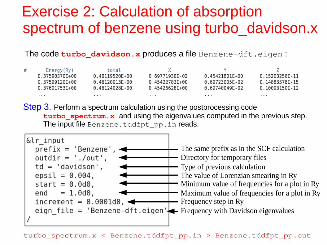
Step 1. Perform an SCF calculation for benzene at the equilibrium structure using the code pw.x

Step 2. Perform Lanczos recursions using the code turbo_lanczos.x The input file is Benzene.lanczos.in :

Exercise 3: Calculation of absorption spectrum of benzene using turbo_lanczos.x

The same prefix as in the SCF calculation Directory for temporary filesThe code writes restart files every restart_step iterationsRestart iterations after previous calculation

Number of Lanczos iterationsPolarization direction of incoming light, 1=x

Exercise 3: Calculation of absorption spectrum of benzene using turbo_lanczos.x

In the output file Benzene.lanczos.out there is information about each

Lanczos iteration :

In the directory out, which contains temporary files, there is a file Benzene.beta_gamma_z.1 which contains the information about Lanczos

coefficients:

Note! The calculation will be a bit too long: 35 minutes using 2 cores.

Therefore, let us see the output files in the directory reference.

Exercise 3: Calculation of absorption spectrum of benzene using turbo_lanczos.x

Step 3. Perform a spectrum calculation using the postprocessing code turbo_spectrum.x and using the Lanczos coefficients computed in the previous step. The input file Benzene.tddfpt_pp.in reads:

The same prefix as in the SCF calculation Directory for temporary files

The value of Lorenzian smearing in RyMinimum value of frequencies for a plot in Ry Maximum value of frequencies for a plot in Ry Frequency step in Ry

Number of calculated Lanczos coefficient Number of extrapolated Lanczos coefficient Type of extrapolation (bi-constant)

Polarization direction (same as in turbo_lanczos.x)

Exercise 3: Calculation of absorption spectrum of benzene using turbo_lanczos.x

The code turbo_spectrum.x produces a file Benzene.plot which can be

used for plotting the absorption spectrum :

Step 4. Plot the spectrum using gnuplot and the script plot_spectrum.gnu

You should obtain the same excitation peak in the spectrum as was obtained using the code turbo_davidson.x in the exercise2 including interaction. The script plot_spectrum.gnu will do such a comparison, and it will produce the file Benzene_spectrum.eps which you can visualize.

Exercise 3: Calculation of absorption spectrum of benzene using turbo_lanczos.xComparison of the absorption spectrum of benzene computed using turbo_lanczos.x and using turbo_davidson.x both including the interation (file Benzene_spectrum.eps):

Exercise 3: Calculation of absorption spectrum of benzene using turbo_lanczos.xturbo_lanczos.x allows us to obtain the absorption spectrum in a wide frequency range just by repeating a postprocessing calculation using turbo_spectrum.x in a larger frequency range. This cannot be done with turbo_davidson.x

Comparison of the absorption spectra of benzene and naphthalene

In naphthalene the pi-orbitals are more delocalized than in benzene, which leads to smaller energy gap, and which hence red-shifts the peaks.

Comparison of the absorption spectra of benzene using local and non-local XC functionals

Hybrid exchange-correlation functionals open the energy gap and blue-shift the peaks (SCF: input_dft='PBE0', Lanczos: d0psi_rs=.true. and the molecule must be centered in the supercell)

Exercise 4: Convergence of the absorption spectrum of Na2

Go to the directory with the input files:

cd Part2_absorption_spectra/exercise4

Study the convergence of the absorption spectrum of Na2 with respect to:

● The number of Lanczos iterations itermax = 50, 100, 150,... without using the extrapolation extrapolation = 'no'

● How many Lanczos iterations is needed to converge the spectrum when the extrapolation is used extrapolation = 'osc'?

● The size of the supercell celldm(1) = 20, 30, 40, ...

Exercise 4: Convergence of the absorption spectrum of Na2

Exercise 4: Convergence of the absorption spectrum of Na2

Behaviour of Lanczos coefficients

Exercise 4: Convergence of the absorption spectrum of Na2

Extrapolation of the Lanczos chains

In the Liuoville-Lanczos approach, the absorption coefficient is computed as:

where is the tridiagonal matrix composed of the Lanczos coefficients.

Extrapolation

Exercise 4: Convergence of the absorption spectrum of Na2