Tutorial: Measurement of fluorescence spectra and de-

termination of relative fluorescence quantum yields of

transparent samples

Marcia Levitus. School of Molecular Sciences and The Biodesign Institute. Arizona StateUniversity, Tempe, AZ, USA.

Abstract

The measurement of fluorescence spectra and the determination of fluorescence quantumyields in transparent samples are conceptually simple tasks, but these procedures are subjectto several pitfalls that can lead to significant errors. Available technical reports and protocolsoften assume that the reader possesses a solid theoretical background in spectroscopy andhas ample experience with fluorescence instrumentation, but this is often not the case giventhe many applications of fluorescence in diverse fields of science. The goal of this tutorialis to provide a didactic treatment of the topic that will hopefully be accessible to readerswithout extensive expertise in the field of fluorescence. The article covers the theoreticalbackground needed to understand the origins of the most common artifacts researchers canexpect. Possible artifacts are illustrated with examples to help readers avoid them or identifythem if present. A step-by-step example of a fluorescence quantum yield determination insolution is provided with detailed experimental information to help readers understand howto design and analyze experiments.

1 Introduction

The popularity of fluorescence-based techniques in fields spanning materials to biology con-tinues to grow with the ever-increasing developments in single-molecule detection and super-resolution microscopy [1–5]. The brightness of a fluorophore at a particular excitation wave-length (λEx), which in general terms measures the ability of a molecule to emit light viaphoto-excitation, is commonly defined as the product of the molar absorption coefficient(ε(λEx)) and the fluorescence quantum yield (φf ) [6]. The fluorescence quantum yield is thefraction of absorbed photons that are emitted as fluorescence, so this parameter is one of thefactors that determine the number of photons that can be detected experimentally and itis therefore intimately related to the limit of detection in fluorescence spectroscopy. Hence,the experimental determination of φf is a critical step in the characterization of fluorescentmolecules and materials. Moreover, accurate determinations of φf are needed for the quanti-tative interpretation of FRET (Forster resonance energy transfer) data. FRET is a populartool in the biosciences that is commonly used to measure inter-molecular distances [3, 7].Fluorescent donor and acceptor probes for FRET are often extrinsic fluorophores attachedto amino acids and nucleobases. The determination of the donor-acceptor distance requires

1

previous knowledge of a parameter known as Forster’s distance (R0, defined as the donor-acceptor distance that results in 50 % energy transfer efficiency), which depends on thefluorescence quantum yield of the donor [8–10]. Although R0 values are easy to find in web-sites and textbooks, these values are most commonly calculated from φf values measuredin solution. Fluorescence quantum yields are often affected by the dye’s environment (e.g.polarity, viscosity, pH, and specific interactions with amino acids or nucleobases) [8, 9, 11],so the rigorous interpretation of FRET data requires the experimental determination of φf(and therefore R0) for the probes incorporated in the biomolecules of interest.

Conceptually, the determination of the fluorescence quantum yield of a transparent sam-ple is relatively simple. Yet, the accurate determination of φf is surprisingly challenging.This tutorial aims to provide readers with the tools necessary to carry out accurate relativequantum yield determinations in transparent samples. There are many excellent techni-cal reports and protocols that describe proper experimental procedures and recommendedstandards [12–15], but these sources assume that readers have expertise with fluorescencetheory and instrumentation. The goal of this tutorial is to provide a didactic treatmentof the topic that will hopefully be accessible to readers with little expertise in the field offluorescence. Readers seeking complementary information or a more thorough theoreticalbackground are encouraged to read the textbooks by J. R. Lakowicz [8], B. Valeur and M.Berberan-Santos [9], and D. Jameson [16].

2 Background

State diagrams such as the one shown in Fig. 1A (frequently called Jablonski diagrams) arecommonly used to depict molecular states and photophysical processes. Thick horizontallines represent molecular electronic states while thin lines represent vibrational states. Solidarrows are used to indicate radiative processes (absorption and emission), and wavy arrowsindicate nonradiative transitions. With very few exceptions, the lowest electronic state ofan organic molecule is a singlet state (labeled as S0 in Fig. 1A). In a typical fluorescenceexperiment, a light source such as a laser or a lamp is used to excite a molecule to the firstelectronic excited state (denoted by S1). Transitions to different vibrational states within thefirst electronic excited state are allowed (see 1O in Fig. 1A), but in solution, molecules relaxrapidly (in picoseconds) to the lowest vibrational level of the first electronic excited stateby transferring excess vibrational energy to the solvent molecules (vibrational relaxation,2O in Fig 1A). Further relaxation to the ground state occurs over longer timescales, usually

tens of picoseconds to hundreds of nanoseconds, depending on the molecule and conditions.Emission of photons accompanying the relaxation of the first electronic excited state to theground state is called fluorescence (See 3O, Fig. 1A). Importantly, S1 can be depopulatedby other mechanisms that do not involve the emission of light (non-radiative processes), andaccordingly, only a fraction of the absorbed photons results in emission of fluorescence pho-tons. Non-radiative processes include internal conversion, intersystem crossing to the tripletstate, energy transfer to another molecule, etc. Readers interested in learning more aboutthe nature of the different non-radiative mechanisms that lead to the relaxation of electronic

2

excited states are encouraged to read references [9, 17]. Because the focus of this article isfluorescence emission, we will consider all other deactivation mechanisms collectively andfocus on the efficiency of fluorescence emission relative to all non-radiative paths combined.

For a given photon absorption event, the fate of the excited state depends on the relativekinetic rates of the different processes that deactivate the excited state. One can envisionthe fate of an excited state as a random event with many outcomes: fluorescence, internalconversion, intersystem crossing, or some other non-radiative process (Fig. 1B). The prob-ability of each outcome depends on how the rate of that particular process compares to therates of all deactivation processes combined. For instance, the probability that the singletexcited state will deactivate by emission of a photon, i.e. fluorescence, is given by the rate offluorescence emission (kf ) divided by the sum of the rates of all the processes that contributeto the deactivation of the excited state (kf +Σknr, where the sum combines all non-radiativeprocesses).

S0

S1

2

1

ISC

T1

3

ExcitedState (S )1

GroundState (S )0

hnexc

S +0 hnem

T1

S +0 D

etc

non-r

adia

tive

path

ways

fluorescence

A B

kf

Sknrý

þ

ü ýþ

ük k

f nr+S

S0

2

2

4

Figure 1: A Simplified Jablonski diagram depicting molecular states and photophysical processes. Onlythe first singlet excited state (S1), and only a few vibrational states are shown for clarity. Absorption 1Oand Fluorescence 3O are radiative processes, depicted in blue and red, respectively. Vibrational relaxation isindicated with wavy vertical arrows, 2O. Internal conversion, 4O, is an isoenergetic nonradiative transitionbetween the lowest vibrational level of S1 and an excited vibrational state of S0 (note that the higherenergy vibrational states of S0 are shown only on the left-side of the figure for clarity). Internal conversionis followed by vibrational relaxation within the S0 manifold, 2O . ISC denotes intersystem-crossing, aradiationless process that leads to the creation of the triplet state. B Cartoon depiction of the possiblepathways by which the first excited state can deactivate, highlighting the random nature of the process. Theprobability that the excited state deactivates via fluorescence is given by the ratio of kf to kf + Σknr, whereΣknr represents the sum of the rate constants of all the non-radiative pathways that can deactivate S1. Thesymbol ∆ represents heat (vibrational energy).

The fluorescence quantum yield, φf , is the quantity that measures the probability thatthe excited state of a molecule will deactivate to the ground state with emission of a photon.A value of φf = 0.8, for example, indicates that the molecule will deactivate with emissionof fluorescence with 80% probability, leaving the remaining 20% probability to all otherdecay mechanisms combined. If a single molecule were excited continuously, this probabilitytranslates into an average of 80 emitted photons per 100 photons absorbed. This definitionestablishes the basis for the optical measurement of the fluorescence quantum yield: φf isthe number of photons emitted as fluorescence (Nf ) over a given time period, divided by the

3

number of photons that were absorbed (NA):

φf =Nf

NA

(1)

From a practical perspective, the measurement of Nf would require the detection of allemitted photons, which cannot be achieved using conventional fluorescence spectrometersbecause these instruments are designed to detect only a fraction of the emitted light. Weshould note that the absolute measurement of a fluorescence quantum yield can be achievedusing instruments equipped with an integrating sphere detector [18, 19]. Absolute measure-ments φf are gaining popularity, but integrating spheres are still considered sophisticatedaccessories and are not widespread. For this reason, in this tutorial we will focus on theoptical determination of relative fluorescence quantum yields, which can be accomplishedwith conventional spectrofluorimeters readily available to most researchers. In brief, relativemeasurements rely on the comparison between the fluorescence signal from the sample ofinterest and the signal from a sample of known φf . If the sample and reference are mea-sured under the same conditions, the same (unknown) fraction of the emitted photons willbe measured in both cases, allowing the determination of one fluorescence quantum yieldrelative to the other (see below).

In addition to optical methods, which rely on the detection of the emitted photons,fluorescence quantum yields can also be determined indirectly by measuring the amountof excitation energy that is converted into heat and dissipated into the solvent. Examplesof calorimetric methods are thermal lensing and photoacoustic spectroscopy, and readersinterested in these techniques are referred to references [20–23].

As stated above, φf is the number of photons emitted as fluorescence divided by thenumber of photons absorbed (Eq. 1). We have already established that conventional spec-trofluorimeters are not able to measure the total number of the emitted photons (Nf ), butonly an unknown fraction k determined by a series of factors that include the solid anglethrough which the instrument collects light, the transmission efficiency of various opticalcomponents, and the quantum efficiency of the detector. Therefore, the number of photonsdetected by the instrument is Nf,d = kNf . As it will become evident as we progress throughthis tutorial, attempting to characterize this fraction is far from straightforward due to themany factors that contribute to it. This limitation is circumvented by performing an ex-periment with a reference sample of known φf in conditions that ensure that the fractionof photons detected for the unknown sample (S) and the reference (R) remains the same.Under these conditions, the ratio of the number of photons detected for the sample andreference (NS

f,d/NRf,d) equals the ratio of the number of photons emitted (NS

f /NRf ), and we

can write

φSfφRf

=NSf /N

SA

NRf /N

RA

=NSf,d/N

SA

NRf,d/N

RA

(2)

Eq. 2 seems straightforward, but we still need to relate the variables involved in theequation (Nf,d, NA) with quantities that can be easily measured using conventional spec-trophotometers and spectrofluorimeters. Spectrophotometers measure the absorbance of the

4

sample, which is related to the fraction of the incident light that is transmitted by the sample(i.e. the transmittance). Most commonly, spectrofluorimeters measure an electric signal inarbitrary units that is proportional to the number of photons detected at the wavelengthdetermined by the emission monochromator of the instrument. Our next step is therefore todescribe the relationship between the experimental observables (absorbance and fluorescenceintensity) and the variables involved in the calculation of φSf /φ

Rf (NA and Nf,d, Eq. 2).

Let us first focus on the quantity Nf,d. When the fluorescence intensity of a sample isrecorded using a spectrofluorimeter, the sample is continuously excited by the excitationsource (usually a lamp) and molecules experience large numbers of successive excitation-emission cycles. Photons emitted as fluorescence have a distribution of energies (and there-fore wavelengths) that reflect the probability of the various transitions from the lowest vi-brational level of the first excited electronic state to different vibrational levels of the groundstate. This energy distribution defines the fluorescence spectrum (often called the emissionspectrum) of the compound, which can be measured using a conventional spectrofluorimeter.

In practice, the fluorescence intensity is measured at a given combination of excitationand emission wavelengths, λEx and λEm, respectively. To acquire the entire fluorescencespectrum, the instrument is set at a given λEx value and λEm is scanned to cover thewhole fluorescence spectrum. As mentioned above, not all emitted photons are detected;the instrument collects fluorescence over a given solid angle, only a fraction of the photonscollected is transmitted through the optical components of the detection system, and finally,only a fraction of the photons that reach the detector generates an electric response. As aconsequence, the total number of photons detected is only a fraction of the number of photonsemitted by the sample at all wavelengths, (Nf in Eq. 1). Let us define the fluorescenceintensity, If (λEx, λEm), as the number of photons detected at wavelength λEm, so thatthe integral of the measured spectrum,

∫∞0 If (λEx, λEm)dλEm represents the total number of

detected photons including all wavelengths (Nf,d). Using the definition of φf (Eq. 1), wecan write: ∫ ∞

0If (λEx, λEm)dλEm = kNf = kNAφf (3)

where the limits of integration indicate that all photons emitted should be counted regardlessof their energy. In practice, as discussed in section 4.2.7, integration is performed over afinite wavelength range. The constant k in Eq. 3 represents the fraction of all emittedfluorescence photons that are detected, and so far, we have assumed that this quantity doesnot depend on emission wavelength. However, as we will discuss in section 3, this is neverthe case. The transmission efficiency of the diffraction gratings used in the monochromatorsof most instruments and the response of the photomultiplier tubes used as detectors are bothwavelength-dependent, and therefore the fraction of photons detected is not constant acrossthe fluorescence spectrum. The quantity If (λEx, λEm) in Eq. 3 is therefore not the measuredfluorescence intensity, but a fluorescence intensity that has been obtained after correctingthe measured value for the wavelength-dependent efficiency of the detection system. Section3 describes the experimental considerations and corrections needed to obtain the correctedspectrum that should be used in Eq. 3.

We will next turn our attention to the quantity NA. The number of photons absorbed

5

during the experiment depends on the absorbance of the solution at the excitation wavelengthused to acquire the fluorescence spectrum (λEx). Indeed, the absorbance of the sample definesa relationship between the intensity of the incident light, I0(λEx), and the intensity absorbedby the sample, IA(λEx):

IA(λEx) = I0(λEx)(1− 10−A(λEx)) (4)

To derive Eq. 4, we used the definition of absorbance (A = − log(IT/I0)), and the factthat the absorbed intensity is the difference between the intensity of the incident light andthe intensity of the transmitted light (IA(λEx) = I0(λEx) − IT (λEx)). Therefore, the term(1 − 10−A(λEx)) represents the fraction of the incident photons that are absorbed by thesample at a given excitation wavelength. The number of photons absorbed by a solution canthen be expressed as NA(λEx) = N0(λEx)(1−10−A(λEx)), where N0 is the number of incidentphotons.

Eq. 3 can be now written as∫ ∞0

If (λEx, λEm)dλEm = kN0(1− 10−A(λEx))φf (5)

The numerical value of the proportionality constant k is generally unknown and depends ona large number of instrumental conditions that are hard to quantitate and reproduce. There-fore, the value of the measured intensity has no real meaning, and it is generally expressedin arbitrary units. However, if the fluorescence spectra of the sample and the reference areacquired using identical experimental conditions (including excitation wavelength, cuvettesize and geometry, slit bandwidths, etc), the values of k and N0(λEx) can be regarded asequal and the ratio of the integrated corrected emission spectra can be expressed as∫∞

0 ISf (λEx, λEm)dλEm∫∞0 IRf (λEx, λEm)dλEm

=(1− 10−A

S(λEx))φSf(1− 10−AR(λEx))φRf

(6)

We stress that Eq. 6 was derived under the assumption that the two measurements (i.e.the sample and reference emission scans) capture the same fraction of the emitted light.This is in part determined by the solid angle through which the instrument collects light,which depends on the refractive index of the solvent (n). The light emitted as fluorescencerefracts at the surfaces separating the solution, the cuvette, and air, and consequently thefluorescence flux that falls on the aperture of the detection channel of the instrument dependson the refractive index of the solvent [8, 24]. If the solvents used to prepare the referenceand sample solutions have different refractive indices, the fraction of photons collected inthe two experiments can be significantly different. To correct for this difference, a correctionfactor that depends on the square of the refractive indices must be included in Eq. 6, whichwritten in terms of φSf /φ

Rf becomes:

φSfφRf

=n2S

n2R

×∫∞0 ISf (λEx, λEm)dλEm∫∞0 IRf (λEx, λEm)dλEm

× (1− 10−AR(λEx))

(1− 10−AS(λEx))(7)

The values of n for common solvents are listed in the Supplemental Information File.

6

We note that the ratio (1−10−AS(λEx))

(1−10−AR(λEx))is often approximated by the ratio AS(λEx)

AR(λEx), and

while the approximation may not result in a significant error at the low absorbance valuesused in the experiments (typically A < 0.04, see below), the calculation of the term (1 −10−A

S(λEx)) in Eq. 7 is straightforward and is always preferred. An explanation of the originof this approximation is provided in the Supplemental Information File (see section S2).In addition, a common misconception is that the calculation of φSf requires comparing thefluorescence output of the sample with a reference of equal concentration. Eq. 7 showsthat the only variable of interest is the absorbance of the solution, which can be measureddirectly with a conventional spectrophotometer. The absorbance of the solution is of courserelated to the concentration of fluorophores as described by Beer-Lambert’s law, but it alsodepends on the extinction coefficient of the compound at the wavelength of excitation. Thefluorescence intensity of a solution of a fluorescent compound will be negligible if excited ata wavelength where the compound does not absorb (small extinction coefficient), regardlessof its concentration.

Eq. 7 is the basis for the measurement of relative fluorescence quantum yields. Althoughthe determination of φSf appears to be relatively simple, it requires a judicious choice of φfreference and measurement conditions, and it is prone to numerous artifacts that will bediscussed in detail in the next sections of the tutorial.

3 Measuring Fluorescence Spectra

The determination of φSf relative to a known standard according to Eq. 7 requires the mea-surement of the complete fluorescence spectrum of the unknown sample and the referenceunder conditions that ensure that the same fraction of the emitted photons are detectedat all times. Specifically, this fraction should not depend on emission wavelength, andshould be the same for the two measurements (i.e. sample and reference). Operating aconventional spectrofluorimeter is surely simple from the technical point of view, but mea-suring fluorescence spectra under these strict conditions is not. There are sample-relatedand instrument-related factors that can contribute to the measurement of distorted spectra(that is, the fraction of the emitted photons that are detected by the instrument varies de-pending on λEm). Similarly, sample-related and/or instrument-related factors can result indifferent fractions of photons detected during the acquisition of the sample and the referenceemission spectra. While some artifacts can be prevented by carefully choosing reagents andexperimental conditions, some are inherent to the instrument and need to be corrected forduring or after the measurement.

3.1 Instrumental Factors

There are several instrumental factors that can result in distortions of the measured spectra.For instance, spectral shifts can occur if monochromators are not properly calibrated, anddistortions can occur if the detection system does not operate within its linear range. Thesecan be easily prevented by taking basic precautions, as described below. The most important

7

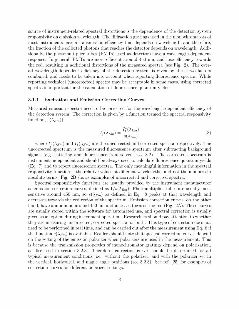
source of instrument-related spectral distortions is the dependence of the detection systemresponsivity on emission wavelength. The diffraction gratings used in the monochromators ofmost instruments have a transmission efficiency that depends on wavelength, and therefore,the fraction of the collected photons that reaches the detector depends on wavelength. Addi-tionally, the photomultiplier tubes (PMTs) used as detectors have a wavelength-dependentresponse. In general, PMTs are more efficient around 450 nm, and lose efficiency towardsthe red, resulting in additional distortions of the measured spectra (see Fig. 2). The over-all wavelength-dependent efficiency of the detection system is given by these two factorscombined, and needs to be taken into account when reporting fluorescence spectra. Whilereporting technical (uncorrected) spectra may be acceptable in some cases, using correctedspectra is important for the calculation of fluorescence quantum yields.

3.1.1 Excitation and Emission Correction Curves

Measured emission spectra need to be corrected for the wavelength-dependent efficiency ofthe detection system. The correction is given by a function termed the spectral responsivityfunction, s(λEm)):

If (λEm) =Iuf (λEm)

s(λEm)(8)

where Iuf (λEm) and If (λEm) are the uncorrected and corrected spectra, respectively. Theuncorrected spectrum is the measured fluorescence spectrum after subtracting backgroundsignals (e.g scattering and fluorescence from solvent, see 3.2). The corrected spectrum isinstrument-independent and should be always used to calculate fluorescence quantum yields(Eq. 7) and to report fluorescence spectra. The only meaningful information in the spectralresponsivity function is the relative values at different wavelengths, and not the numbers inabsolute terms. Fig. 2B shows examples of uncorrected and corrected spectra.

Spectral responsitivity functions are usually provided by the instrument manufactureras emission correction curves, defined as 1/s(λEm). Photomultiplier tubes are usually mostsensitive around 450 nm, so s(λEm) as defined in Eq. 8 peaks at that wavelength anddecreases towards the red region of the spectrum. Emission correction curves, on the otherhand, have a minimum around 450 nm and increase towards the red (Fig. 2A). These curvesare usually stored within the software for automated use, and spectral correction is usuallygiven as an option during instrument operation. Researchers should pay attention to whetherthey are measuring uncorrected, corrected spectra, or both. This type of correction does notneed to be performed in real time, and can be carried out after the measurement using Eq. 8 ifthe function s(λEm) is available. Readers should note that spectral correction curves dependon the setting of the emission polarizer when polarizers are used in the measurement. Thisis because the transmission properties of monochromator gratings depend on polarization,as discussed in section 3.2.3. Therefore, correction curves should be determined for alltypical measurement conditions, i.e. without the polarizer, and with the polarizer set inthe vertical, horizontal, and magic angle positions (see 3.2.3). See ref. [25] for examples ofcorrection curves for different polarizer settings.

8

500 550 600 650 700 7500.0

0.2

0.4

0.6

0.8

1.0

300 400 500 600 7000

5

10

15

20

Nor

mal

ized

Flu

ores

cenc

e In

tens

ity

Wavelength (nm)

A B

Fl Cy3 Cy5

1/s(

em)

Wavelength (nm)

Figure 2: AEmission correction curve for a PTI Quantamaster 4/2005SE instrument equipped with aHamamatsu R928 PMT. B Uncorrected (black) and corrected (red) spectra for dilute solutions of fluorescein(Fl, in 0.1 M NaOH), Cy3 (in EtOH) and Cy5 (in EtOH).

The most common method for measuring the emission correction curve is to use a cali-brated light source placed at the sample position and to compare the measured emission withthe certified data for the actual lamp spectral output. This requires a high level of expertiseand should be preferably done by specialized technicians. Most companies that commercial-ize spectrofluorimeters can perform this type of calibration as an optional on-site service.Alternatively, the correction curve can be determined by acquiring the spectra of standardcompounds for which the corrected emission spectra are known. Corrected emission spectrafor several compounds are available in Appendix 1 of Ref. [8], and a kit certified by BAM(Bundesanstalt fur Materialforschung und -prufung, Germany) is currently commerciallyavailable and can be used to cover the 300-770 nm spectral range [26].

Readers should be aware that spectral responsivity functions are sometimes given inpower units instead of photon units because data for the spectral distribution of tungstenlamps is usually provided in the form of energy units per unit wavelength interval [27].This can lead to confusion because converting between energy and photon units requiresmultiplication by λ (E = hc/λ), so the shape of the spectral responsivity function is different.The correction curves of most modern spectrophotometers are already provided in photonicunits, so this particular issue is typically not a concern. A quick test to ensure that thecorrection curve provided by the manufacturer is in photonic units is to measure the spectrumof a standard substance, and use Eq. 8 to obtain the corrected spectrum. If the spectrumobtained in this way is grossly distorted it may be an indication that the correction curvewas provided in energy units and a conversion using Plank’s equation is need.

In addition to the correction curves discussed above, spectrofluorimeters are equippedwith a reference channel (usually a quantum counter or a photodiode) that monitors thelamp’s output in real time during the measurement. This is used to monitor possible fluctua-tions in the intensity of the lamp, and more importantly, to correct for wavelength-dependent

9

variations in I0. This is critical for the acquisition of excitation spectra, but unimportant inthe determination of relative quantum yields provided that both the sample and referenceare excited at the same wavelength. Researchers should note that both types of corrections(excitation and emission) are often available as options within the software, and may notbe selected by default.Researchers should also be aware that built-in (i.e. vendor-provided)emission correction curves may not span the whole wavelength range accessible by the in-strument.

3.1.2 Detection System Linearity

Most spectrofluorimeters are equipped with photo multiplier tubes (PMTs), which are knownto be nonlinear at high intensities of incident light. Instrument manufacturers often recom-mend maximum intensities to ensure that measurements are within the linear range of theinstrument, and measuring within this range is critical to ensure that the intensity measuredby the instrument is proportional to the fluorescence intensity emitted by the sample. Themost straightforward method to determine the linear intensity range of the detection systemof a given instrument is to prepare a series of solutions by serial dilution and to verify thatthe measured intensity is proportional to concentration. It is important to use solutionswith low absorbance (A < 0.04) to avoid deviations due to inner filter effects (see 3.2.2), orotherwise, measured intensities will not be linear even if the system is operating within thedetection linear range.

3.1.3 Wavelength Accuracy

In general, there is no need to re-validate wavelength accuracy in commercial instrumentsunless users suspect problems with the calibration of the monochromators. The most obviousmanifestation of a potential problem with wavelength accuracy is a systematic shift in theacquired excitation and/or emission corrected spectra. The corrected emission spectra ofseveral fluorescent standards can be found in Appendix 1 of Ref. [8], and these can be usedto assess the wavelength accuracy of the instrument if needed. Because the fluorescencespectra of molecular species in solution are rather wide, a more precise method for theassessment of wavelength accuracy is to use the peak positions of the atomic lines of lowpressure atomic lamps (often called pen lamps) [28]. These pens are inexpensive and readilyavailable from vendors that specialize in light sources for research applications.

The position of the Raman peak can be also used to assess the accuracy of one monochro-mator with respect to the other [28]. The water Raman peak appears at a fixed positionwith respect to the wavelength of the excitation beam (see section 3.2.1), so this is an inex-pensive and straightforward method to evaluate wavelength accuracy in the UV region of thespectrum (Raman intensities are too weak in the visible). Similarly, the scattering intensityfrom a dilute scattering solution in a standard cuvette can be used to assess a possible biasbetween the two wavelength selectors. The position of the scattering peak (Rayleigh scatter-ing, see 3.2.1) should coincide with the wavelength of the exciting beam, and any differenceindicates that one or both monochromators require re-calibration.

10

3.2 Sample Factors

3.2.1 Rayleigh and Raman Scattering

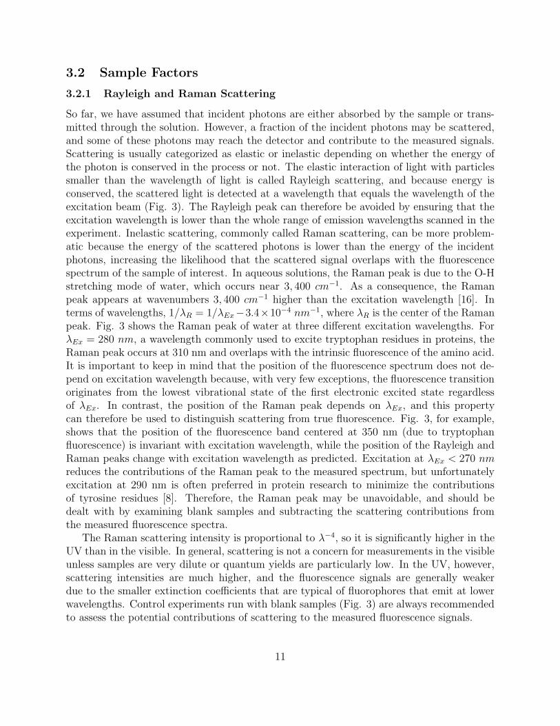
So far, we have assumed that incident photons are either absorbed by the sample or trans-mitted through the solution. However, a fraction of the incident photons may be scattered,and some of these photons may reach the detector and contribute to the measured signals.Scattering is usually categorized as elastic or inelastic depending on whether the energy ofthe photon is conserved in the process or not. The elastic interaction of light with particlessmaller than the wavelength of light is called Rayleigh scattering, and because energy isconserved, the scattered light is detected at a wavelength that equals the wavelength of theexcitation beam (Fig. 3). The Rayleigh peak can therefore be avoided by ensuring that theexcitation wavelength is lower than the whole range of emission wavelengths scanned in theexperiment. Inelastic scattering, commonly called Raman scattering, can be more problem-atic because the energy of the scattered photons is lower than the energy of the incidentphotons, increasing the likelihood that the scattered signal overlaps with the fluorescencespectrum of the sample of interest. In aqueous solutions, the Raman peak is due to the O-Hstretching mode of water, which occurs near 3, 400 cm−1. As a consequence, the Ramanpeak appears at wavenumbers 3, 400 cm−1 higher than the excitation wavelength [16]. Interms of wavelengths, 1/λR = 1/λEx−3.4×10−4 nm−1, where λR is the center of the Ramanpeak. Fig. 3 shows the Raman peak of water at three different excitation wavelengths. ForλEx = 280 nm, a wavelength commonly used to excite tryptophan residues in proteins, theRaman peak occurs at 310 nm and overlaps with the intrinsic fluorescence of the amino acid.It is important to keep in mind that the position of the fluorescence spectrum does not de-pend on excitation wavelength because, with very few exceptions, the fluorescence transitionoriginates from the lowest vibrational state of the first electronic excited state regardlessof λEx. In contrast, the position of the Raman peak depends on λEx, and this propertycan therefore be used to distinguish scattering from true fluorescence. Fig. 3, for example,shows that the position of the fluorescence band centered at 350 nm (due to tryptophanfluorescence) is invariant with excitation wavelength, while the position of the Rayleigh andRaman peaks change with excitation wavelength as predicted. Excitation at λEx < 270 nmreduces the contributions of the Raman peak to the measured spectrum, but unfortunatelyexcitation at 290 nm is often preferred in protein research to minimize the contributionsof tyrosine residues [8]. Therefore, the Raman peak may be unavoidable, and should bedealt with by examining blank samples and subtracting the scattering contributions fromthe measured fluorescence spectra.

The Raman scattering intensity is proportional to λ−4, so it is significantly higher in theUV than in the visible. In general, scattering is not a concern for measurements in the visibleunless samples are very dilute or quantum yields are particularly low. In the UV, however,scattering intensities are much higher, and the fluorescence signals are generally weakerdue to the smaller extinction coefficients that are typical of fluorophores that emit at lowerwavelengths. Control experiments run with blank samples (Fig. 3) are always recommendedto assess the potential contributions of scattering to the measured fluorescence signals.

11

300 400 5000.0

2.0x105

4.0x105300 400 500

0.0

2.0x105

300 400 5000.0

2.0x105

4.0x105

300 400 500

300 400 500

300 400 500

Fluo

resc

ence

Inte

nsity

(A.U

)

ex = 290 nm

ex = 280 nm

ex = 270 nm

Wavelength (nm)

Rayleigh peak

Raman peak

Tryptophan in water Water

Figure 3: Uncorrected emission spectra of a c.a. 1µM solution of Tryptophan in water showing the Rayleighand Raman peaks. Excitation wavelengths were 270 nm (top), 280 nm (middle) and 290 nm (bottom). Thesignals measured with pure water in the cuvette under identical conditions are shown on the right

3.2.2 Inner Filter Effects

The absorbance of a solution defines a relationship between the intensity of the incidentlight (I0) and the intensity of the transmitted light (IT ), and is proportional to the sampleconcentration (C), the extinction coefficient (ε), and the path length (b):

A (λ) = −log(IT (λ) /I0 (λ)) = b.ε (λ) .C (9)

Consider a 1 cm×1 cm cuvette in an instrument with the traditional right-angle geometry.The detection channel of the instrument is focused at the center of the cuvette, so mostphotons collected by the instrument are emitted by molecules close to the central part ofthe cuvette. We can picture the solution as being composed of layers or slabs (Fig. 4).If I0 denotes the incident excitation intensity for the layer that faces the lamp, then theincident intensity for the layer in the middle of the cuvette (0.5 cm) is the transmittedintensity from the previous layer, equal to I010−0.5.ε.C = I010−A/2 where A is the absorbanceof the solution measured with the 1 cm path length cuvette (Eq. 9). If the absorbance ofthe solution at the excitation wavelength is 0.5, the central part of the cuvette would beexcited with an intensity of approximately 10−0.25I0 ≈ 0.56I0. The intensity of fluorescenceis proportional to the intensity of the exciting beam, and the instrument collects photonsemitted from the central part of the cuvette. Therefore, the quantum yield measured inthese conditions would be only about 56 % of the value measured for a very dilute solution.

12

This phenomenon is known as the excitation (or primary) inner filter effect [9, 29], and itsimpact in φf determinations can be minimized by using dilute solutions (A(λEx) < 0.04).

I0

0.56I0

1 cm 0.05 cm 0

0.31I0

A B

Figure 4: A Schematic representation of a solution in terms of slabs or layers. The solution is excitedfrom the right with intensity I0. The incident excitation intensity for each layer is I010−l.ε.C , where l is incentimeters, ε is the extinction coefficient in cm−1M−1, and C is the molar concentration. The values givenin this figure correspond to a solution with A = 0.5 at the excitation wavelength (see text). B Photographof a solution of rhodamine 6G excited with a 532 nm laser pointer. The absorbance of the solution at theexcitation wavelength is approximately 2. Fluorescence (yellow) is observed along the path of the laser.Excitation inner filter effects are manifested as a decrease in fluorescence intensity from right to left.

In addition to the excitation inner filter effect described above, photons emitted by amolecule can be re-absorbed by other molecules before reaching the detector. This effect isknown as the emission (or secondary) inner filter effect [9,29], and results in both a decreasein the total number of photons emitted by the solution, and a distortion of the spectrum.Consider the absorption and emission spectra of rhodamine 6G in ethanol, shown in Fig. 5.The emission spectrum shown in black was obtained with a solution with A ≈ 0.025 at theexcitation wavelength, where inner filter effects can be considered negligible. The emissionspectrum shown in red was measured with a solution about 40 times more concentrated(A ≈ 1 at the excitation wavelength). What is the origin of the apparent shift in the emissionmaximum? In the dilute solution, it is unlikely that a fluorescence photon encounters anothermolecule before reaching the detector, and therefore the probability that the photon is re-absorbed by another molecule in the solution is low. For the concentrated solution, anemitted photon is likely to encounter another molecule before it reaches the detector. Ifthat photon is re-absorbed, the newly formed excited state may deactivate by a mechanismdifferent from fluorescence, and as a consequence the first emission event will not resultin a photon reaching the detector. Importantly, not all photons that collide with othermolecules are equally likely to be re-absorbed. Photons emitted on the blue side of thefluorescence spectrum are more likely to be re-absorbed than photons of lower energy (redside) because the former carry energies that match the absorption spectrum of the substance(see Fig. 5, blue curve). Indeed, the shape of the fluorescence spectrum of the concentratedsolution matches the spectrum of the dilute solution at wavelengths higher than 575 nm,where the extinction coefficient of this dye is very small. At these emission wavelengths,emitted photons may encounter other molecules, but the probability of re-absorption is very

13

small. The largest discrepancy between the two emission spectra is found at wavelengthswhere rhodamine 6G absorbs efficiently, as seen in Fig. 5. These distortions give rise to anapparent spectral shift to the red, as shown in the inset of Fig. 5. The effect of self-absorptionon the measured spectrum depends on the absorbance of the sample at the wavelengths ofthe emitted photons. Therefore, it will be more notorious for dyes with small Stokes shifts(large overlap of absorption and emission spectra).

400 450 500 550 600 650 700 7500.0

0.5

1.0

1.5

2.0

2.5

500 600 7000.0

0.5

1.0

Fluo

resc

ence

Inte

nsity

(A.U

.)

Wavelength (nm)

Figure 5: Absorption (blue curve) and corrected fluorescence spectra of Rhodamine 6G in ethanol. Theabsorption spectrum was scaled arbitrarily. The emission spectra shown in black and red were measuredwith solutions with an absorbance A ≈ 0.025 and A ≈ 1 at the excitation wavelength (495 nm), respectively.The spectra are shown in arbitrary units, and were multiplied by arbitrary constants to match at the redside of the spectrum. Inset: Emission spectra of the same solutions normalized to a peak maximum of 1.

3.2.3 Polarization Effects

Let us reiterate that the use of Eq. 7 requires that the measurements of the fluorescencespectra of the unknown sample and the reference are performed under conditions that en-sure that the same fraction of the emitted photons are detected at all times. We havealready discussed the instrumental factors that result in wavelength-dependent variations inthe transmission and detection of the emitted photons, and how to correct for them. Here,we will discuss polarization effects, which in general lead to the measurement of an intensitythat is not truly proportional to the total fluorescence intensity emitted by the sample. Animportant conclusion of this discussion is that polarization artifacts are important even whenno polarizers are used in the experiment, and that the use of polarizers in particular orien-tations is needed to avoid polarization artifacts in quantitative fluorescence measurements.

14

One common approach to eliminate polarization effects is to place a polarizer in the verticalposition in the excitation path, and a polarizer set at the magic angle (54.7◦) in the emissionpath. The reasons behind this requirement are examined below in detail.

Polarization is a property of light that refers to the direction of the oscillating electricfield. In the case of linearly polarized light, the electric field oscillates in a single directionperpendicular to the direction of light propagation. The lamps used in most fluorimeters emitnatural (unpolarized) light, which is characterized by a random direction of the electric field.Physically, unpolarized light can be described as a mixture of two independent light streamswith equal intensity but perpendicular polarizations (Fig. 6). To understand polarizationeffects, let us first discuss what happens when we excite the solution with linearly polarizedlight. To do this, one must use a polarizer to isolate one particular direction of the oscillatingelectric vector of the exciting light, as shown in Fig. 6. In solution, molecules are expectedto be oriented randomly, but only those properly oriented relative to the electric vectorof the polarized excitation light can absorb a photon. Readers may be familiar with theconcept of transition dipole moment for an electronic transition, which is a quantity relatedto the extinction coefficient that determines the probability that the molecule will absorblight. However, while the extinction coefficient is a scalar quantity (a number), the transitiondipole moment is an oscillating vector that has a defined direction on the nuclear frameworkof the molecule [8, 9, 17]. For the dye Cy3, for example, the transition dipole moment forabsorption in the visible lies along the long axis of the molecule as shown in Fig. 6 [30].The probability that a molecule will absorb a photon is proportional to cos2θ, where θ isthe angle between the incident electric field and the absorption transition dipole momentof the molecule (see Fig.S2). This means that molecules with absorption transition dipolemoments aligned parallel to the electric vector of the incident light (molecule B in Fig. 6)have the highest probability of absorption, whereas molecules with absorption transitiondipole moments aligned perpendicular to the electric vector of incident light (molecule A inFig. 6) do not absorb at all. Molecule C in Fig. 6 will have a lower probability of absorptionthan molecule B, and will therefore contribute less to the total number of emitted photons.

Let us assume for a moment that molecules re-orient slowly so that emission occurs fromthe same orientation the molecule had when the photon was absorbed. For a single molecule,fluorescence emission is polarized along the transition dipole moment that corresponds tofluorescence emission. For Cy3, the emission transition dipole moment is almost parallel tothe absorption dipole moment [30], so we can assume that emission is polarized along thelong axis of this molecule. Consider now a solution of Cy3 in a highly viscous solvent thatprevents molecular rotation during the lifetime of the excited state. Because molecules incertain orientations are more likely to absorb light, the overall fluorescence emission will bepartially polarized even if the molecules themselves are randomly distributed in the solution.The polarization of the fluorescence emission can be analyzed in terms of three orthogonalcomponents (Iz, Iy, Ix, Figure 6). If the excitation polarizer is set in the vertical positionas shown in Fig. 6, molecules with orientations close to this axis (e.g. molecule B) aremore likely to absorb, and emission will be preferentially polarized along the vertical axis aswell (that is, Iz will be larger than Ix and Iy). Fluorescence will not be perfectly polarized

15

A

B

C

Natural light

exc. polariz

er

Vertically

polarized lig

htSample

Iz

To detector

em. polarizer

VV HIy

Ix

NN

Figure 6: Left: Schematics of a fluorescence measurement using polarizers in the excitation and emissionpaths. The polarizer in the excitation path (left side of the cuvette) is used to select vertically-polarized lightfrom the natural light emitted by the lamp. The polarization of the fluorescence emission is analyzed in termsof three orthogonal components (Iz, Iy, Ix). Iz and Iy are measured when the emission polarizer (right sideof the figure) is placed in the vertical or horizontal positions, respectively. Ix cannot be measured. Right:A Cy3 molecule. The arrow on the molecule represents the orientation of the transition dipole moment forabsorption in the visible band (see text). The probability of absorption is proportional to cos2θ, where θ isthe angle between the line defined by the transition dipole moment and the electric field of the incident light

along the vertical axis because molecules with other orientations, such as molecule C, stillabsorb light (although with a lower probability). If molecule C does not re-orient during itsexcited state, it will emit from an orientation that will lead to Iy ≈ Iz because it is at anapproximately 45° angle with respect to the vertical axis.

The intensities along the z and y directions can be measured by placing a polarizer in theemission path in the vertical or horizontal position, respectively (Fig. 6). Critical for thisdiscussion, the component along the direction of propagation of the emitted light (Ix) cannotbe detected, and this in fact is the key to understand the origin of polarization artifacts whenno polarizers are used. We will first consider the intensities measured when the excitationand emission polarizers are placed in vertical (V) or horizontal (H) positions. The measuredintensities will be denoted IV V , IV H , IHV , IHH , where the first and second subscripts indicatethe orientations of the excitation and emission polarizer, respectively. For the example above(vertical excitation, no re-orientation), we concluded that IV V > IV H .

The degree of polarization of the emitted light is usually analyzed in terms of a quantityknown as fluorescence anisotropy, defined as

r =IV V − IV HIV V + 2IV H

(10)

In practice, a correction known as the G-factor is needed because monochromator gratingsdo not transmit vertically and horizontally polarized light with the same efficiency (seeSupplemental Information, Section S3.2). In the case of fluorophores with emission transitiondipole moments that lie in the same direction as the absorption transition dipole moments,the measured fluorescence anisotropy is expected to be r = 0.4 if molecules do not re-orientduring the lifetime of the excited state [8, 9, 16]. This value is positive because fluorescencemostly arises from molecules oriented parallel to the excitation light, which is verticallypolarized. However, r is lower than 1 because molecules such as molecule C in Fig. 6 still

16

contribute to the fluorescence signal, and emit light that is not perfectly aligned with thevertical axis of the emission polarizer (i.e. Iy is not zero).

In general, unless the fluorophore is embedded in a a rigid matrix such as a solid or aglass, or measurements are performed at very low temperatures, molecules will re-orient intimescales comparable to the lifetime of the excited state. Rotational diffusion during thelifetime of the excited state results in a partial depolarization of the emitted light [8,9]. Forinstance, consider molecule B in Fig. 6, which absorbs with the highest probability due toits initial orientation. If the molecule rotates while in the excited state, fluorescence will beemitted from other orientations, decreasing IV V and increasing IV H . In terms of Eq. 10, itis evident that rotational diffusion results in a reduction of r. For example, the fluorescenceanisotropy values of aqueous solutions of the dyes Cy3 and Cy3B at room temperature arer = 0.25 and r = 0.045, respectively [31]. The difference is due to the significantly differentfluorescence lifetimes of the two dyes (τCy3 = 0.18 ns and τCy3B = 2.7 ns) [31]. The valuemeasured for Cy3B, which is close to zero, indicates that rotational diffusion is much fasterthan fluorescence emission, so that molecules emit from all orientations with almost the sameprobability, and IV V ≈ IV H . For Cy3, the almost identical rotational diffusion time resultsin only a partial depolarization of the emitted light due to the much shorter fluorescencelifetime.

How is this discussion relevant to the measurement of φf? In general, the total intensityis IT = Ix + Iy + Iz, but except for specific configurations of the polarizers, the measuredintensity is a fraction of this value that depends on the degree of polarization of the emittedlight (quantified by r). To start, imagine that you are interested in measuring the fluorescencequantum yield of Cy3 relative to Cy3B. Suppose for the moment that you perform themeasurements with polarizers placed in the vertical position in both the excitation andemission channels. For vertically polarized excitation, the z − axis is an axis of symmetryand Iy = Ix (see section S3.1, Supplemental Information file). With this in mind, the totalintensity can be expressed in terms of the two measured components (IV V = Iz, IV H = Iy)as IT = IV V + 2IV H . Algebraic manipulation of Eq. 10 gives, IV V = (2r + 1)/3 × IT , andtherefore, for this configuration of polarizers, the measured intensity (IV V ) would be onlya fraction of the total intensity. This on its own is not problem, except that this fractiondepends on the degree of polarization of the emitted light, which is different for the sampleand the reference. For the Cy3 solution (r = 0.25), IV V ≈ 0.5IT , and for the Cy3B solution(r = 0.045), IV V ≈ 0.36IT . Therefore, in this case, a higher fraction of the total photonsemitted would be measured for the sample (Cy3) than for the reference (Cy3B), resulting ina calculated φCy3f about 1.4 times greater than the actual value.

One can naively think that this bias disappears if the emission polarizer is omitted fromthe measurement, but one must remember that Ix cannot be detected, so the measured in-tensity would be Im = Iz + Iy = IV V + IV H , which is still a fraction of IT that depends on r.Algebraic manipulation of Eq. 10 gives, IV H = (1−r)/3×IT , so Im/IT = IV V /IT +IV H/IT =(2 + r)/3 (see Supplemental Information, Section S3.1). If fluorescence is completely depo-larized (r = 0), Iz = Iy = Ix and Im/IT = 2/3 consistent with the fact that one of the threeidentical components is not detected. If r 6= 0, the fraction of the total intensity that is

17

measured depends on the value of r.At this point it may seem that the solution is to remove both the excitation and the

emission polarizers. In this case, the measured intensity is still Iz + Iy because Ix cannotbe detected, and as shown in the Supplemental Information file (section S3.1), Im/IT =(Iz + Iy)/(Iz + Iy + Ix) = (4 − r)/6, which still depends on the value of r. However,because 0 ≤ r ≤ 0.4, polarization effects are in principle expected to be rather small.Yet, the situation is further complicated by the fact that monochromator gratings do nottransmit vertically and horizontally polarized light with equal efficiency. Therefore, evenwithout polarizers, the sample is excited with partially polarized light and detected with apolarization bias, and artifacts can indeed be significance (see section 5.5.5).

How can polarizers help remove polarization artifacts? It can be shown that the useof polarizers in certain orientations allow the detection of a signal that is still a fractionof IT , but importantly, this fraction is independent of r. The most common approachto achieve this goal is to place the excitation polarizer in the vertical position and theemission polarizer at the so-called magic angle (φ ≈ 54.7◦), defined as cos2φ = 1/3. Readersinterested in a derivation for the magic angle conditions are encouraged to read refs. [8, 9].Some instruments have only basic settings for the polarizers, and researchers may find thatthey can only select the vertical and horizontal position, but not the needed 54.7◦. In thiscase, the total fluorescence intensity can be calculated from the measured IV V and IV Hintensities as IT = IV V + 2IV H . However, this requires a correction for the polarization-dependent sensitivity of the detection system (known as the G-factor). For details, see theSupplementary Information File, section S3.2.

4 Measuring Relative Fluorescence Quantum Yields

4.1 Fluorescence Quantum Yield Standards

The precision with which the fluorescence quantum yield of the unknown sample can bedetermined using Eq. 7 ultimately depends on the accuracy of the value of φRf used inthe calculation. Values of φf found in the literature can be surprisingly different even forcommon compounds that have been widely investigated for decades. For example, literaturevalues of φf for quinine bisulfate in H2SO4 vary from 0.508 to 0.65 [32]. In general, variationsmay be due to instrumental factors (e.g. inaccurate spectral corrections, see 3.1.1), purityof dyes and solvent, inner filter artifacts (3.2.2), polarization artifacts (3.2.3), or variationsin temperature, pH, ionic strength, etc. Researchers should be therefore wary of the manyindividual measurements published in the literature, and instead rely on values compiled inauthoritative sources such the publications and reports from IUPAC (International Unionof Pure and Applied Chemistry, USA), BAM (Bundesanstalt fur Materialforschung und -prufung, Germany), or NIST (National Institute of Standards and Technology, USA) [12,14, 33]. The compounds recommended in these publications have been chosen as standardsbecause their fluorescence quantum yields have been investigated systematically with respectto variables such as temperature, excitation wavelength, chromophore concentration, etc.

18

Importantly, publications from these reputable sources often contain information about theuncertainty of the recommended φf which reflects the spread of all reliable published valuesby individual researchers. Examples of recommended standards are shown in Fig. 7 (see Fig.S4 for structures and more information), and readers are encouraged to consult references[12,14,33] for a more comprehensive list of φf standards. According to an IUPAC report [14],quinine sulfate in H2SO4 is the most popular standard for φf determinations, even in caseswhere the sample emits in a significantly different region of the spectrum. The readershould note that while quinine sulfate is still a recommended standard [12], the recommendedsolvent is perchloric acid. The φf of quinine sulfate displays a more pronounced temperaturedependence in sulfuric acid than in perchloric acid [34], so the latter is recommended tominimize uncertainties in the measurements.

250 300 350 400 450 500 550 600 650 700 750 800 8500.0

0.2

0.4

0.6

0.8

1.0

250 300 350 400 450 500 550 600 650 700 750 800 8500.0

0.2

0.4

0.6

0.8

1.0

250 300 350 400 450 500 550 600 650 700 750 800 8500.0

0.2

0.4

0.6

0.8

1.0

250 300 350 400 450 500 550 600 650 700 750 800 8500.0

0.2

0.4

0.6

0.8

1.0

250 300 350 400 450 500 550 600 650 700 750 800 8500.0

0.2

0.4

0.6

0.8

1.0

250 300 350 400 450 500 550 600 650 700 750 800 8500.0

0.2

0.4

0.6

0.8

1.0

Nor

mal

ized

Abs

orba

ce/

Nor

mal

ized

Flu

ores

cenc

e In

tens

ity

Wavelength (nm)

Quinine Sulfate0.105 M HClO4

f = 0.59

Nor

mal

ized

Abs

orba

ce/

Nor

mal

ized

Flu

ores

cenc

e In

tens

ity

Wavelength (nm)

Coumarin 153Ethanol

f = 0.53

Nor

mal

ized

Abs

orba

ce/

Nor

mal

ized

Flu

ores

cenc

e In

tens

ity

Wavelength (nm)

Fluorescein0.1 M NaOH

f = 0.925

Nor

mal

ized

Abs

orba

ce/

Nor

mal

ized

Flu

ores

cenc

e In

tens

ity

Wavelength (nm)

Rhodamine 6GEthanol

f = 0.91

Nor

mal

ized

Abs

orba

ce/

Nor

mal

ized

Flu

ores

cenc

e In

tens

ity

Wavelength (nm)

Rhodamine 101Ethanol

f = 0.915

Nor

mal

ized

Abs

orba

ce/

Nor

mal

ized

Flu

ores

cenc

e In

tens

ity

Wavelength (nm)

Oxazine 1Ethanol

f = 0.15

Figure 7: Normalized absorption and corrected emission spectra of some recommended fluorescence quan-tum yield standards. The structures of the dyes are compiled in the supplemental information file. The φfvalues indicated in each case were obtained from reference [12] (except for fluorescein, see refs. [14, 35])

One of the main criteria for choosing the reference is that ideally, the standard andsample should absorb and emit in the same spectral regions. Eq. 7 was derived under theassumption that the value of N0(λEx) in Eq. 5 remains the same during the acquisition of the

19

sample and the reference emission spectrum. Because the photon flux of the lamp generallydepends on wavelength, a correction for the wavelength-dependence of the exciting photonflux would be required if the excitation wavelength used for the sample and for the referenceare not the same. This can be done if necessary [13], but should be avoided if possible tominimize the number of factors that contribute to inaccuracies in the measured quantumyield. In addition, as discussed in section 3.1.1, correction curves are needed to obtain thecorrected fluorescence spectra from the measured signals. In principle, correction would notbe needed if the two solutions (sample and reference) had identical emission spectra. Becausethis is rarely the case, it is always preferable to use a reference with an emission spectrumsimilar to that of the unknown sample. This does not eliminate the need for correctingthe measured spectra, but minimizes the effects of any inaccuracies that may be introducedduring the correction step.

4.2 Experimental Procedures and Considerations

4.2.1 Sample Preparation

High-purity dyes and solvents must always be used to avoid the interference of contami-nants. HPLC or spectrophotometric grade solvents are best, but even then, it is alwaysgood practice to measure the absorption and fluorescence spectra of the solvent to rule outpotential impurities and verify its suitability for the fluorescence experiments. All glasswareor plasticware used in sample preparation must be cleaned with care, and samples used forquantum yield determinations must be made fresh if possible. For solutions that have beenstored, it is good practice to measure the absorbance spectrum of the solution to rule outpossible degradation. For instance, the author has observed a steep decrease in the ab-sorbance in the visible (but not in the UV) of buffered solutions of DNA labeled with thedye Cy5 stored for several months at −20 °C in the dark. While these storing conditions aretypical for DNA samples, the Cy5 molecule seems to undergo an irreversible (and certainlyunexpected) transformation.

Reference solutions for the determination of relative φf values are commonly preparedby dissolving the reference dye in a pure solvent. Novice researchers are often tempted toweigh a quantity of the solid to prepare such solutions, but the quantities needed to preparea few milliliters of a solution with a measurable absorbance (A < 1) are often too small forthe sensitivity of common analytical scales. For example, to prepare 2 mL of a solution oftetramethylrhodamine with a peak absorbance of A = 1, one would need to weigh about 8µg of solid. Knowledge of the concentration is not needed to calculate φf , so there is no needto measure the mass of dye used in the preparation of the solution. Instead, it is sufficient tograb a very small particle of solid with a needle or a pipette tip, and dissolve it in the desiredsolvent. If the absorbance of this solution is too high, as is frequently the case, successivedilutions should be made until the desired absorbance is achieved.

20

4.2.2 Cuvettes

A variety of cuvettes for fluorescence spectroscopy are available from vendors that specializein laboratory equipment. Cuvettes may differ in optical length, volume, shape and thematerial of the optical windows. Most cuvettes are made of glass or quartz. Althoughglass is cheaper, it absorbs strongly in the UV limiting the use of these cuvettes to the range360–2,500 nm. Quartz cuvettes, on the other hand, can be used down to 200 nm, enabling themeasurement of important biological molecules such as tryptophan. Except for specializedcuvettes (e.g. for front-face fluorescence measurements), fluorescence cuvettes generally havean external 1 cm × 1 cm square cross section and at least three optical windows. Twooptical windows are on parallel faces of the cuvette and used to measure the transmittance(and therefore the absorbance) of the solution. At least one of the perpendicular faces ofthe cuvette (and often both) contain optical windows for fluorescence measurements usinginstruments with a 90° geometry. Depending on the cuvette, the path length along thesetwo directions may be different. For instance, the three cuvettes shown in Fig. 8 have a1 cm-path length in the direction orthogonal to the plane of the figure, but different pathlengths in the perpendicular direction. The cuvette shown in the middle has optical windowsin all four faces, and can be used in absorbance measurements in either direction (albeitwith different optical path lengths). The cuvette shown on the right has only three opticalwindows, while the fourth side of the cuvette is not transparent (see Fig. 8D). This cuvetteneeds to be oriented along the 1 cm-path length direction for absorbance measurements, andthe perpendicular window needs to be oriented towards the emission detection channel forfluorescence.

Figure 8: ATraditional fluorescence cuvette with four optical windows and a 10 mm×10 mm path length.B Semi-micro fluorescence cuvette with a 10 mm×4 mm path length. The bottom of this cuvette is designedto hold a small stirring bar. C Ultra-micro fluorescence cuvette with a 10 mm × 2 mm path length. Thiscuvette has three optical windows (the side facing left is opaque). D Same cuvette rotated clockwise. Thereare two parallel optical windows separated by 1 cm for absorbance measurements (green arrows) and aperpendicular window with a 2 mm path length to measure fluorescence (red arrow)

Most cuvettes do not need to be completely filled, but it is critical that there is enoughsample in the cuvette for the incident light to go through the solution and not air. Standard

21

1cm× 1cm cuvettes require about 2 mL of solution, while ultra-micro cuvettes that requireas little as 12 µL can be purchased from vendors such as Hellma. Ultra-micro cuvetteshave smaller optical windows, so it is critical that the height of the center of the samplecompartment is well aligned with the incident beam. The height of the light beam variesamong different manufacturers of spectrophotometers and spectrofluorimeters, so knowledgeof this height (usually called the z -dimension) is a pre-requisite to select a cuvette compatiblewith a specific instrument. Although working with smaller volumes seems like an obviousadvantage, the small size of the optical window of these cuvettes makes it challenging toobtain accurate and reproducible measurements of absorbance and fluorescence. If possible,it is always better to use a cuvette with an optical window larger than the size of the beam.This will require larger sample volumes, but will minimize uncertainties in all measurements.

4.2.3 Measuring the Absorbance of the Solution

The calculation of φf relies on precise knowledge of the absorbance of both the sample andreference solutions. The measurement of the absorbance of a solution is typically performedwith a spectrophotometer using the same cuvettes that will be used for the acquisition ofthe fluorescence spectra. A double-beam spectrophotometer is the best choice to maximizeanalytical precision, but even then, it is always a good idea to measure the full spectrumof the sample (as opposed to just the absorbance at the desired wavelength) to check forany baseline offsets and for potential contributions of scattering to the baseline. Scatteringoccurs when light interacts with particles smaller than the wavelength of light such as colloids,aggregates or large protein assemblies. The scattering intensity is proportional to the inverseof the fourth power of the wavelength, resulting in a baseline that increases rapidly withdecreasing wavelength. This is illustrated in Fig. 9, which shows the absorption spectra ofSulforhodamine 101 in water together with the spectrum of the same solution containing asmall quantity of colloidal silica. Both spectra were measured using water in the referencecompartment of the spectrophotometer. Scattering is particularly problematic and difficultto correct for in the UV region of the spectrum, so it should be prevented if at all possible.

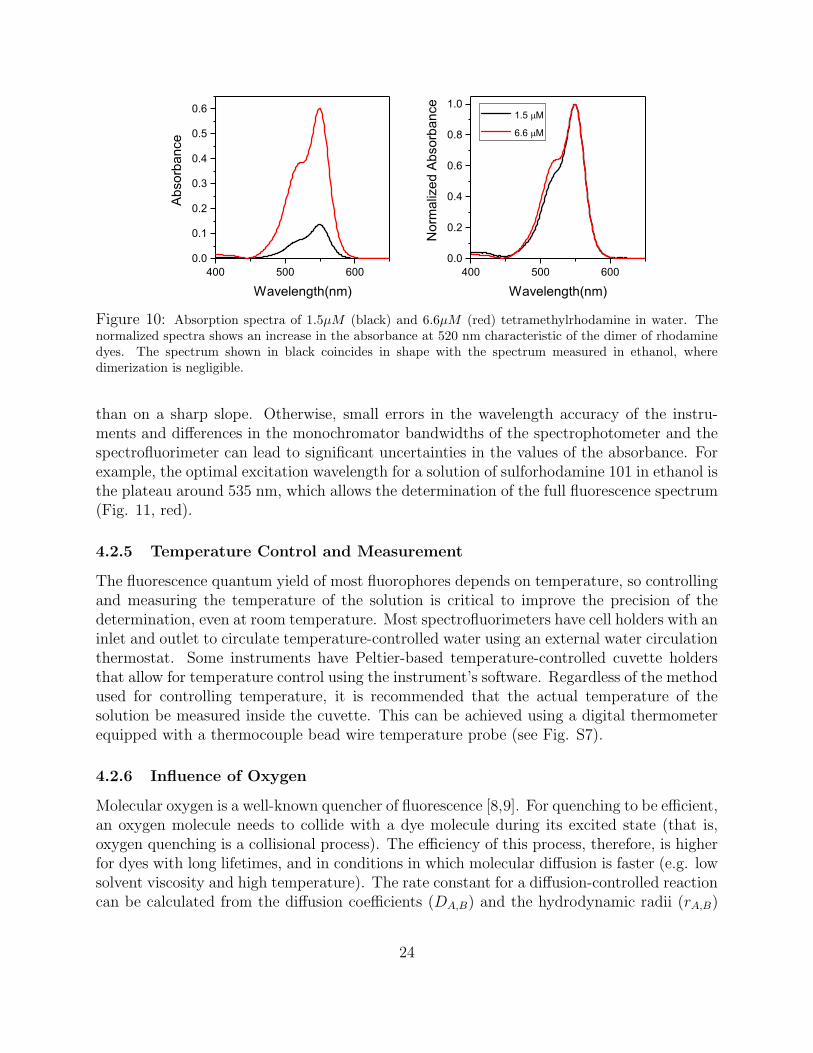
The accuracy of absorbance measurements is best in the range A ≈ 0.5–1, but valueslower than c.a. 0.04 are needed to avoid inner filter effects. Whether the small absorbancevalues needed for the φf determination can be measured directly with precision dependson the quality of the spectrophotometer. Typically, accuracy is improved by measuring theabsorbance of a stock solution with an absorbance in the range A = 0.5–1, and performinga precise dilution to obtain the desired absorbance A < 0.04. This of course relies on theassumption that the absorbance of the solution is linear with concentration in this range. Anobvious control is to verify that the shape of the spectrum of the stock solution is identical tothe shape of the spectrum of the dilute solution except for noise. For example, xanthene dyessuch as fluorescein and rhodamine derivatives form dimeric assemblies in aqueous solutionwith a plane-to-plane stacking geometry (H-dimers) and a characteristic absorption bandthat overlaps with the absorption shoulder of the monomer. As a consequence, the dimeriza-tion of these dyes results in an apparent increase in the absorbance of the monomer [36,37].Fig. 10 illustrates this point. The visible spectrum of a 6.6 × 10−6 M aqueous solution of

22

300 400 500 600 7000.0

0.2

0.4

0.6

0.8

1.0

1.2

1.4

1.6

300 400 500 600 7000.00.20.40.60.81.01.21.41.6

Absorban

ce

Wavelength (nm)

Absorban

ce

Wavelength (nm)

Figure 9: Absorption spectrum of sulforhodamine 101 in water (red) and in water containing a smallquantity of Ludox (colloidal silica, blue curve). Water was used in the reference compartment of the spec-trophotometer in both cases. Inset: “Absorbance” spectrum of the Ludox solution alone. The signal is notdue to absorption, but to the scattering of light by the small colloidal particles (see text).

tetramethylrhodamine has an absorbance of c.a. 0.4 at 520 nm, which would be optimal foran accurate determination. However, a comparison of the normalized spectrum of this solu-tion with the spectrum of a 1.5× 10−6 M solution of the same dye shows the characteristicspectroscopic signature of the dimeric form of rhodamine, i.e., an increase in the absorbanceof the shoulder band. The spectrum of the dilute solution coincides with the spectrum ofthe monomeric form of the dye, but the spectrum of the more concentrated solution showsa clear contribution from the dimer. As a consequence, the absorbance of these solutionsis not proportional to the concentration of dye, and the dilution step recommended abovewould lead to an erroneous estimate of the absorbance of the dilute solution.

4.2.4 Choosing the Excitation Wavelength

The determination of φf requires integration of the whole fluorescence spectrum of both thesample and the reference solutions. This requires an excitation wavelength that is shortenough so that the whole emission spectrum can be scanned without interference from theRayleigh scattering peak discussed in section 3.2.1. A common mistake is to excite at theabsorption maximum of the chromophore, but this often results in the truncation of the fluo-rescence spectrum on the high-energy (low-wavelength) side (Fig. 11, inset). Another crite-rion for the selection of the excitation wavelength is the precision with which the absorbancecan be determined, which depends on the slope (steepness) of the absorption spectrum at thewavelength of interest. Absorbance measurements are more precise when taken on a plateau

23

400 500 6000.0

0.1

0.2

0.3

0.4

0.5

0.6

400 500 6000.0

0.2

0.4

0.6

0.8

1.0

Abso

rban

ce

Wavelength(nm)

1.5 M

6.6 M

Nor

mal

ized

Abs

orba

nce

Wavelength(nm)

Figure 10: Absorption spectra of 1.5µM (black) and 6.6µM (red) tetramethylrhodamine in water. Thenormalized spectra shows an increase in the absorbance at 520 nm characteristic of the dimer of rhodaminedyes. The spectrum shown in black coincides in shape with the spectrum measured in ethanol, wheredimerization is negligible.

than on a sharp slope. Otherwise, small errors in the wavelength accuracy of the instru-ments and differences in the monochromator bandwidths of the spectrophotometer and thespectrofluorimeter can lead to significant uncertainties in the values of the absorbance. Forexample, the optimal excitation wavelength for a solution of sulforhodamine 101 in ethanol isthe plateau around 535 nm, which allows the determination of the full fluorescence spectrum(Fig. 11, red).

4.2.5 Temperature Control and Measurement

The fluorescence quantum yield of most fluorophores depends on temperature, so controllingand measuring the temperature of the solution is critical to improve the precision of thedetermination, even at room temperature. Most spectrofluorimeters have cell holders with aninlet and outlet to circulate temperature-controlled water using an external water circulationthermostat. Some instruments have Peltier-based temperature-controlled cuvette holdersthat allow for temperature control using the instrument’s software. Regardless of the methodused for controlling temperature, it is recommended that the actual temperature of thesolution be measured inside the cuvette. This can be achieved using a digital thermometerequipped with a thermocouple bead wire temperature probe (see Fig. S7).

4.2.6 Influence of Oxygen

Molecular oxygen is a well-known quencher of fluorescence [8,9]. For quenching to be efficient,an oxygen molecule needs to collide with a dye molecule during its excited state (that is,oxygen quenching is a collisional process). The efficiency of this process, therefore, is higherfor dyes with long lifetimes, and in conditions in which molecular diffusion is faster (e.g. lowsolvent viscosity and high temperature). The rate constant for a diffusion-controlled reactioncan be calculated from the diffusion coefficients (DA,B) and the hydrodynamic radii (rA,B)

24

500 600 7000.0

0.2

0.4

0.6

0.8

1.0

1.2

500 600 700

ex = 535 nm

ex = 576 nm

Nor

mal

ized

Abs

orba

nce

Wavelength (nm)

535 nm

576 nm

0.0

0.2

0.4

0.6

0.8

1.0

1.2

Nor

mal

ized

Flu

ores

cenc

e In

tens

ity

Figure 11: Normalized absorption and emission spectrum of sulforhodamine 101 in ethanol. The curvein red was obtained exciting at 535 nm, which allows the acquisition of the full emission spectrum. Inset:Excitation at the absorption peak (576 nm) forces the researcher to start the emission scan at λEm > 576nm,which results in a truncated spectrum.

of the two interacting molecules (in this case, molecular oxygen and the fluorophore), and isof the order of k = 1010M−1 s−1 for oxygen in water at room temperature. Assuming thatquenching is a diffusion-controlled process, as has been demonstrated for aromatic hydro-carbons [38], the product k[O2] is a pseudo-first order reaction constant for the quenchingof fluorescence by oxygen. For water in equilibrium with the atmosphere, the concentrationof dissolved oxygen is 2.7 × 10−4 M , which gives k[O2] ≈ 3 × 106 s−1. For quenching tobe efficient, this rate needs to be comparable or greater than the rate of fluorescence emis-sion, which is given by the inverse of the fluorophore’s lifetime. In other words, the valueof 1/k[O2] ≈ 330 ns needs to be similar or smaller than the lifetime of fluorescence of thedye. Consistent with this, quenching by dissolved oxygen is negligible for most commonfluorophores, which have lifetimes of the order of a few nanoseconds, but very efficient forfluorophores such as pyrene, which have lifetimes in the hundreds of nanoseconds [8, 9]. Ifneeded, the concentration of oxygen in the solvent can be reduced by bubbling nitrogen orargon gas, or by freeze-pump-thaw cycling.Regardless of the method, degassing can causeconcentration changes that need to be accounted for by measuring the absorbance of thedegassed solution in a well-sealed cuvette.

25

4.2.7 Integration of the Corrected Fluorescence Spectrum

The focus so far has been on ensuring that the measured fluorescence spectrum is an accuraterepresentation of the true fluorescence spectrum of the sample. This requires a careful choiceof experimental conditions and the use of correction factors. Once this is accomplished, thecalculation of φf according to Eq. 7 requires the integration of the measured corrected fluo-rescence spectrum. Integration should be performed as a function of wavelength (as opposedto wavenumber) because all instruments are equipped with grating monochromators, andthese operate at a constant wavelength bandpass. The limits of integration in 7 indicatethat all photons emitted by the sample should be counted regardless of their energy. Inpractice, however, integration over an infinite wavelength range is neither feasible nor ap-propriate. The limits of integration should be wide enough to cover the whole spectrum, butalso limited to avoid unnecessary contributions of background, scattering, or other spuriouscontributions to the signal. The software that comes with most instruments usually includesintegration tools that can be used to calculate the integral of the measured corrected spec-trum. Otherwise, various computer programs such as Origin, Igor Pro or Sigmaplot includesimilar integration tools. Because fluorescence spectra are usually measured in 0.5 or 1 nmsteps, several hundreds of points are collected during the scan and the area under the curve(i.e. the needed integral) can be approximated by adding the values of all the measuredintensities and multiplying the result by the size of the wavelength acquisition step used inthe experiment (e.g. 0.5 nm). For example, for the fluorescence spectrum shown in Fig. 11,this method results in an estimated area that is only 5 × 10−3% different from the valueobtained by integrating the curve using mathematical software.

5 A step-by-step example

In this section we will walk the reader through an example to illustrate how to implementthe information provided in previous sections. All files acquired in the experiments describedbelow are provided as supplementary information. Let us assume that we are interested indetermining the fluorescence quantum yield of the dye Cy3 (nonsulfonated, see Fig. S4)in 50% (V/V) glycerol, and for the purpose of this exercise, let us assume there is nospectroscopic data reported in the literature for this compound.

5.1 Preparation of the solution of interest

We are interested in determining the fluorescence quantum yield of Cy3 in 50% glycerol.The 50% (V/V) glycerol solution (solvent) was prepared by mixing equal volumes of doublydistilled water and pure glycerol (Alfa Aesar, spectrophotometric grade). As mentioned insection 4.2.1, just a few micrograms of the solid are needed to prepare the solution, but thismass does not need to be measured or known. Accordingly, to prepare the solution, we justgrabbed a barely visible amount of solid with a pipette tip, and dissolved the solid in 2 mLof 50% (V/V) glycerol.

26

5.2 Initial spectroscopic characterization

We are assuming that no spectroscopic data is available for this compound, so we needto acquire preliminary absorption and emission spectra to be able to choose an appropriatequantum yield reference. We do not need rigorous conditions yet (e.g. magic angle conditionsor temperature control), but the absorbance of the solution needs to be kept at a reasonablevalue to avoid re-absorption effects that can distort spectra severely (see section 3.2.2). Basedon our experience, we avoid using small-volume cuvettes unless absolutely necessary, so forthis determination we chose standard 1cm × 1cm quartz fluorescence cuvettes (Fig. 8, see4.2.2). The absorbance spectrum of the sample prepared in 5.1 was acquired using 50% (V/V)glycerol solution in the reference channel of the spectrophotometer (Fig. 12). As discussedin section 4.2.4, spectral shoulders are usually good choices for λEx, but the absorbanceof this solution is about an order of magnitude higher than the values recommended tominimize inner-filter effects (section 3.2.2). For this reason, we made a dilution to obtain anabsorbance of approximately 0.05 at the shoulder of the spectrum, and then measured theemission spectrum of this dilute solution exciting at 514 nm (the shoulder of the absorptionspectrum). The measured preliminary emission spectrum is shown in Fig. 12. The goalof this step is just to inspect the spectrum of the unknown sample to have the informationneeded to choose an appropriate quantum yield standard, so we did not use polarizers, andwe did not control the temperature of the cuvette. In this step, it is only important toavoid artifacts that can greatly distort the shape of the spectrum, such as re-absorption(emission inner filter effect) or working above the linear range of the detector (section 3.1.2).Accordingly, the excitation and emission slits were adjusted to ensure that the uncorrectedsignals were within the linear range of the instrument.

5.3 Choice of fluorescence quantum yield standard

A discussion of the considerations that need to be taken into account for choosing a standardwas presented in section 4.1. We inspected the spectral data reported in the references citedin that section (see Fig. 7 for a partial list), and determined that the absorption andemission spectra of the compound rhodamine 6G in ethanol are the closest to the spectraof our sample (Fig. 12). We therefore proceeded to prepare a solution of rhodamine 6G inspectrophotometric grade ethanol following the same procedure reported above for the Cy3solution. The absorption spectrum of this solution (using ethanol in the reference channelof the spectrophotometer) is shown in Fig.13A.

5.4 Preparation of the sample and reference solutions for the φfmeasurements

The solutions prepared initially are too concentrated for a φf determination. As explainedin this tutorial, it is best to keep the absorbance of the solutions lower than c.a. 0.04 at theexcitation wavelength to minimize inner filter effects (section 3.2.2), but as shown in Fig.13A, the absorbance values of both solutions are too high by over an order of magnitude.

27

400 450 500 550 600 650 700 7500.0

0.2

0.4

0.6

0.8

1.0

Abso

rban

ce

Wavelength (nm)

0.0

0.2

0.4

0.6

0.8

1.0

Nor

mal

ized

Flu

ores

cenc

e In

tens

ity

Figure 12: Absorption and preliminary corrected emission spectra of the Cy3 solution prepared in 5.1(measured in a 1cm × 1cm cuvette). Absorbance values are as measured, while emission intensities werenormalized to a maximum value of 1. The solution was diluted 17-fold prior to the acquisition of the emissionspectrum to minimize inner filter effects. Excitation wavelength was 514 nm.

We note that the initial spectroscopic characterization described above (see 5.2) just requiresthat the absorbance is low enough to avoid distortions in the spectrum (i.e. emission innerfilter effects), but in this step it is also important to avoid excitation inner filter effects. Toachieve the desired low absorbance values, one could dilute the stock solutions and measurethe absorbance again, or rely on the dilution factor to re-calculate the new absorbanceassuming that absorbance is proportional to concentration in the conditions used in theexperiments (section 4.2.3). We have a standard dual-beam UV-VIS spectrophotometer(Shimadzu UV-1700), which is not accurate at the low absorbance values needed for the φfdeterminations. For this reason, we prefer to measure more precise values (around A ≈ 0.5)and perform a precise dilution to obtain the desired absorbance. In this case, we chose toperform a precise 1:25 dilution of the rhodamine solution, and a 1:17 dilution of the Cy3solution. The second dilution factor was chosen so as to match the absorbances of bothsolutions as much as possible at the wavelengths used to excite the samples during theacquisition of the emission spectra. The calculated absorption spectra of these dilutions areshown in Fig. 13B.

As mentioned in section 4.2.3, one potential concern is dye aggregation, which would re-sult in spectral changes and a non-linear relationship between absorbance and concentration.For this reason, we performed a quick control experiment to verify that the spectrum of Cy3in 50% (V/V) glycerol does not change upon dilution, and that absorbance is proportional to

28

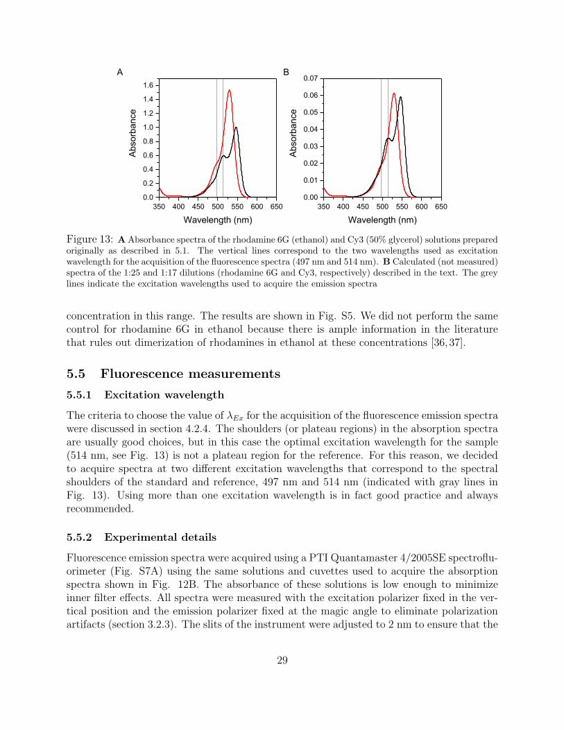
350 400 450 500 550 600 6500.0

0.2

0.4

0.6

0.8

1.0

1.2

1.4

1.6

350 400 450 500 550 600 6500.00

0.01

0.02

0.03

0.04

0.05

0.06

0.07

Absorban

ce

Wavelength (nm)

A B

Absorban

ce

Wavelength (nm)

Figure 13: A Absorbance spectra of the rhodamine 6G (ethanol) and Cy3 (50% glycerol) solutions preparedoriginally as described in 5.1. The vertical lines correspond to the two wavelengths used as excitationwavelength for the acquisition of the fluorescence spectra (497 nm and 514 nm). B Calculated (not measured)spectra of the 1:25 and 1:17 dilutions (rhodamine 6G and Cy3, respectively) described in the text. The greylines indicate the excitation wavelengths used to acquire the emission spectra

concentration in this range. The results are shown in Fig. S5. We did not perform the samecontrol for rhodamine 6G in ethanol because there is ample information in the literaturethat rules out dimerization of rhodamines in ethanol at these concentrations [36,37].

5.5 Fluorescence measurements

5.5.1 Excitation wavelength

The criteria to choose the value of λEx for the acquisition of the fluorescence emission spectrawere discussed in section 4.2.4. The shoulders (or plateau regions) in the absorption spectraare usually good choices, but in this case the optimal excitation wavelength for the sample(514 nm, see Fig. 13) is not a plateau region for the reference. For this reason, we decidedto acquire spectra at two different excitation wavelengths that correspond to the spectralshoulders of the standard and reference, 497 nm and 514 nm (indicated with gray lines inFig. 13). Using more than one excitation wavelength is in fact good practice and alwaysrecommended.

5.5.2 Experimental details

Fluorescence emission spectra were acquired using a PTI Quantamaster 4/2005SE spectroflu-orimeter (Fig. S7A) using the same solutions and cuvettes used to acquire the absorptionspectra shown in Fig. 12B. The absorbance of these solutions is low enough to minimizeinner filter effects. All spectra were measured with the excitation polarizer fixed in the ver-tical position and the emission polarizer fixed at the magic angle to eliminate polarizationartifacts (section 3.2.3). The slits of the instrument were adjusted to 2 nm to ensure that the

29

uncorrected signals (i.e. the signals detected by the instrument) were always lower than themaximum recommended by the manufacturer of our instrument (section 3.1.2). We have in-dependently verified that signals are indeed linear in this recommended range. Temperaturewas controlled using a water circulation system. The inlet and outlet that connect to thesample holder are shown in Fig. S7B. Temperature was measured inside the cuvette usinga digital thermometer with a mm-sized probe (Fig. S7C). In our experience, temperatureshould be measured inside the cuvette placed in the cuvette holder with the lid of the in-strument closed, especially when the thermostat is set at temperatures significantly differentfrom the ambient temperature. For these measurements, we set the thermostat so that thetemperature measured inside the cuvette was 25◦C.

All signals were corrected during the measurement using the emission correction curveprovided by the instrument’s manufacturer, which is stored within the software of the in-strument. The acquired corrected emission spectra are shown in Fig. 14. We also acquiredthe spectra of the two solvents (pure ethanol and 50 % glycerol (V/V), see Fig. S6), anddetermined that these signals were negligible compared to the emission signals of the twofluorescent samples. Otherwise, we would have subtracted the blanks from the measuredspectra before applying spectral corrections.

500 550 600 650 700 7500E+00

1E+06

2E+06

3E+06

4E+06

5E+06

Cy3 in 50% glycerol (V/V) Rhodamine 6G in Ethanol

Fluo

resc

ence

Inte

nsity

(A.U

.)

Wavelength (nm)

Figure 14: Corrected fluorescence emission spectra of Cy3 (in 50% glycerol, black line) and rhodamine 6G(in ethanol, red line) under magic angle conditions. The solutions are the same as the ones used to acquirethe absorption spectra of Fig. 13B. Excitation and emission slits were set at 4 nm. Excitation wavelengthwas 514 nm. Temperature was controlled and measured inside the cuvette as 25◦C.

30

5.5.3 Calculations

The calculation of φSf using Eq. 7 requires integration of the spectra shown in Fig. 14,the values of the two absorbances at the excitation wavelength, literature (or experimental)values of the indices of refraction of the solvents, and an authoritative value of φRf .

We integrated the spectra of Fig. 14 using Origin Pro (see section 4.2.7) and obtained∫∞0 IRf (514nm, λEm)dλEm = 2.223 × 108 for rhodamine 6G and

∫∞0 ISf (514nm, λEm)dλEm =

3.235× 107 for Cy3. The measured absorbances of these samples at 514 nm (Fig. 13B) were0.0349 and 0.0350 for rhodamine 6G and Cy3, respectively. The refractive indices of 50%(V/V) glycerol (sample) and ethanol (reference) are nS = 1.40703 and nR = 1.3611. Usingthese values in Eq. 7, we get:

φSfφRf

=n2S

n2R

×∫∞0 ISf (λEx, λEm)dλEm∫∞0 IRf (λEx, λEm)dλEm

× (1− 10−AR(λEx))

(1− 10−AS(λEx))= 0.155 (11)

Finally, using φRf = 0.91 [12], we get φSf = 0.141.The same procedure with the data acquired using λEx = 497 nm gives φSf = 0.138. The

percent difference between the φSf values obtained at 497 nm and 514 nm is 2.2%. Given theprecision of the reported value of φRf = 0.91 and all the uncertainties in the measurementsinvolved in the calculation of φSf we would report the fluorescence quantum yield of Cy3in 50% glycerol (25 °C) as φf = 0.14. Readers are encouraged to follow common practicesto ensure reproducibility of the results and to estimate the uncertainty of the measurementfrom the standard deviation of as many repeats as possible.

5.5.4 Are spectral corrections necessary?

We repeated the measurements using λEx = 514 nm under magic angle conditions butwe omitted the spectral responsivity corrections in all measurements. The calculated φSfunder these conditions was 0.117, a value c.a. 17% lower than the value measured when theproper spectral corrections are applied. This is not surprising as the emission of the sample(Cy3) is red-shifted with respect to the emission of the reference, and the sensitivity of theinstrument decreases towards the red. Therefore, the Cy3 signals are more underestimatedthan the rhodamine 6G signals, resulting in a lower ratio of the integrated intensities.

5.5.5 Are polarizers necessary?

We repeated the measurements using λEx = 514 nm but omitting the polarizers in boththe excitation and emission channels. The calculated φf under these conditions was 0.117, avalue c.a. 17% lower than the value measured with polarizers. This value is equal to the valueobtained when ignoring spectral correction by coincidence. The fluorescence anisotropies ofthese solutions were measured using Eq. 10 and taking into account the corrections (G-factor) described in the supplemental information section. The measured anisotropies werer = 0.282 and r = 0.019 for the sample and reference, respectively. The relatively high

31

fluorescence anisotropy value for the Cy3 solution is responsible for the polarization artifactsintroduced by not using polarizers during the measurement, as discussed in section 3.2.3.

We also calculated φSf using data acquired without polarizers and without taking intoaccount spectral corrections, and obtained φSf = 0.098, a value c.a. 31% lower than the valuemeasured in 5.5.3. This significant discrepancy highlights the importance of being rigorouswhen using fluorescence as a quantitative tool.

6 Conclusions

The main objective of this tutorial was to provide researchers with the tools needed to avoidcommon artifacts in fluorescence spectroscopy, and to incentivize investigators to evaluaterigorously the variables that affect the quality of the data they report. Although there areseveral resources available to investigators with ample experience with fluorescence tech-niques [13, 15, 28, 39–41], these can be overwhelming to researchers with expertise in otherfields that use fluorescence, but do not have a strong background in this field. The experi-mental acquisition of fluorescence spectra is straightforward from the technical point of view,but as we discussed in this tutorial artifacts are commonplace. One of the most commonpitfalls is illustrated in Fig. 4, which shows severe distortions in the measured spectrum dueto secondary inner filter effects. Reporting uncorrected spectra spectra is also commonplace,but the impact of this depends greatly on the application. It is critical that researchersare clear on whether they publish corrected or uncorrected spectra so readers can evaluatecritically the information that is being reported. For instance, as shown in Fig. 2, the cor-rected and uncorrected spectra of the common FRET dye Cy3 are noticeable different. Thisdifference is significant in the calculation of the FRET overlap integral, which is one of thefactors that determine the value of the Forster distance R0. Raman scattering is anothercommon source of artifacts, especially in the UV region of the spectrum.

The determination of fluorescence quantum yields is also conceptually simple but subjectto many sources of error. Common pitfalls include not using a suitable φf standard, measur-ing in conditions where inner filter effects are significant, and ignoring spectral corrections.As demonstrated in section 5, the use of polarizers in the so-called magic angle conditionsis also important when using samples with large values of fluorescence anisotropy. Some re-searchers wrongly believe that a low fluorescence anisotropy value is guaranteed for organicfluorophores in fluid solution, but this ignores the fact that this is true only for fluorophoreswith relatively long fluorescence lifetimes. As described in our example, the fluorescenceanisotropy of a small dye like Cy3 is relatively large due to the short fluorescence lifetime ofthe dye.

We hope readers will find this tutorial accessible and useful. Those who need moreresources or want to deepen their knowledge of basic concepts of fluorescence are encouragedto read the textbooks by J. R. Lakowicz [8], B. Valeur and M. Berberan-Santos [9], and D.Jameson [16].

32

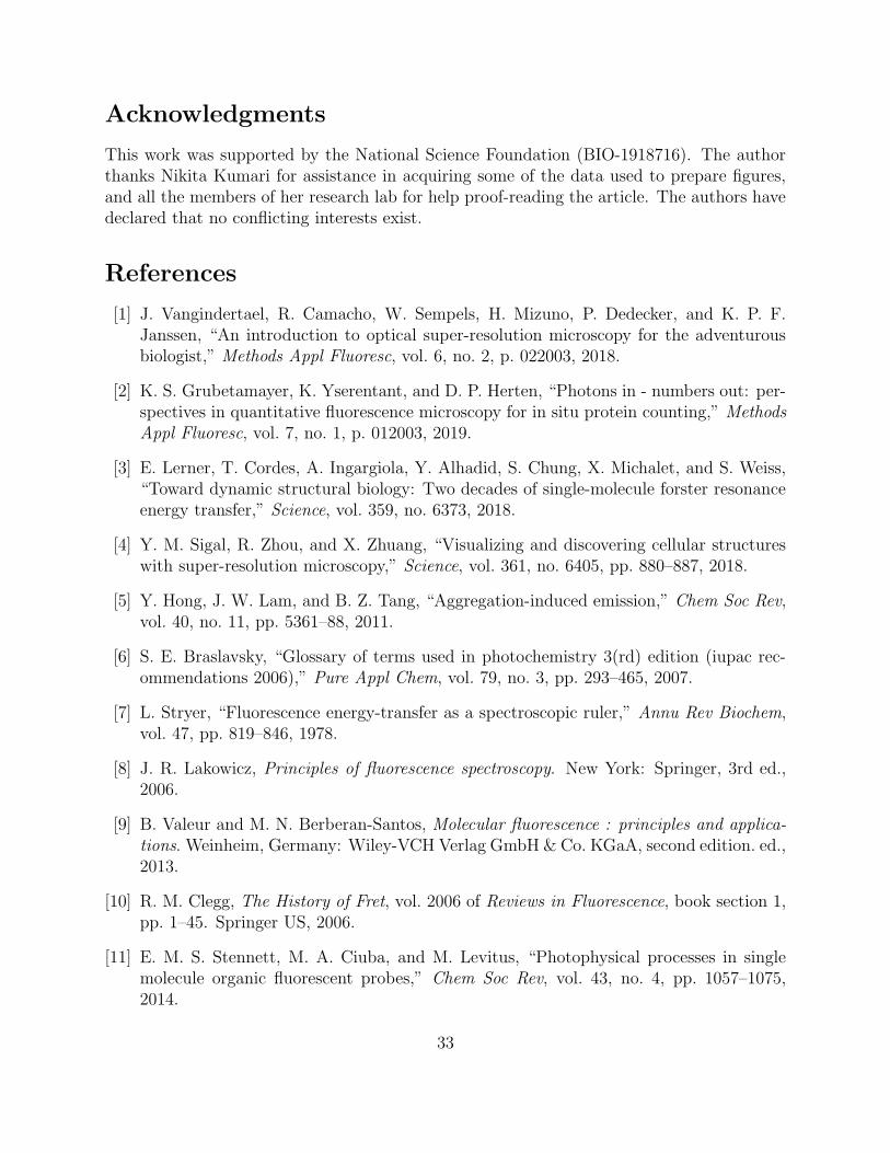
Acknowledgments

This work was supported by the National Science Foundation (BIO-1918716). The authorthanks Nikita Kumari for assistance in acquiring some of the data used to prepare figures,and all the members of her research lab for help proof-reading the article. The authors havedeclared that no conflicting interests exist.

References

[1] J. Vangindertael, R. Camacho, W. Sempels, H. Mizuno, P. Dedecker, and K. P. F.Janssen, “An introduction to optical super-resolution microscopy for the adventurousbiologist,” Methods Appl Fluoresc, vol. 6, no. 2, p. 022003, 2018.

[2] K. S. Grubetamayer, K. Yserentant, and D. P. Herten, “Photons in - numbers out: per-spectives in quantitative fluorescence microscopy for in situ protein counting,” MethodsAppl Fluoresc, vol. 7, no. 1, p. 012003, 2019.

[3] E. Lerner, T. Cordes, A. Ingargiola, Y. Alhadid, S. Chung, X. Michalet, and S. Weiss,“Toward dynamic structural biology: Two decades of single-molecule forster resonanceenergy transfer,” Science, vol. 359, no. 6373, 2018.

[4] Y. M. Sigal, R. Zhou, and X. Zhuang, “Visualizing and discovering cellular structureswith super-resolution microscopy,” Science, vol. 361, no. 6405, pp. 880–887, 2018.

[5] Y. Hong, J. W. Lam, and B. Z. Tang, “Aggregation-induced emission,” Chem Soc Rev,vol. 40, no. 11, pp. 5361–88, 2011.

[6] S. E. Braslavsky, “Glossary of terms used in photochemistry 3(rd) edition (iupac rec-ommendations 2006),” Pure Appl Chem, vol. 79, no. 3, pp. 293–465, 2007.

[7] L. Stryer, “Fluorescence energy-transfer as a spectroscopic ruler,” Annu Rev Biochem,vol. 47, pp. 819–846, 1978.

[8] J. R. Lakowicz, Principles of fluorescence spectroscopy. New York: Springer, 3rd ed.,2006.

[9] B. Valeur and M. N. Berberan-Santos, Molecular fluorescence : principles and applica-tions. Weinheim, Germany: Wiley-VCH Verlag GmbH & Co. KGaA, second edition. ed.,2013.

[10] R. M. Clegg, The History of Fret, vol. 2006 of Reviews in Fluorescence, book section 1,pp. 1–45. Springer US, 2006.

[11] E. M. S. Stennett, M. A. Ciuba, and M. Levitus, “Photophysical processes in singlemolecule organic fluorescent probes,” Chem Soc Rev, vol. 43, no. 4, pp. 1057–1075,2014.

33

[12] C. Wurth, M. Grabolle, J. Pauli, M. Spieles, and U. Resch-Genger, “Relative and abso-lute determination of fluorescence quantum yields of transparent samples,” Nat Protoc,vol. 8, no. 8, pp. 1535–1550, 2013.

[13] U. Resch-Genger and K. Rurack, “Determination of the photoluminescence quantumyield of dilute dye solutions (iupac technical report),” Pure Appl Chem, vol. 85, no. 10,pp. 2005–2026, 2013.

[14] A. M. Brouwer, “Standards for photoluminescence quantum yield measurements in so-lution (iupac technical report),” Pure Appl Chem, vol. 83, no. 12, pp. 2213–2228, 2011.

[15] K. Rurack, Fluorescence Quantum Yields: Methods of Determination and Standards,pp. 101–145. Berlin, Heidelberg: Springer Berlin Heidelberg, 2008.

[16] D. M. Jameson, Introduction to fluorescence. Boca Raton: CRC Press, Taylor & FrancisGroup, 2014.

[17] N. J. Turro, V. Ramamurthy, and J. C. Scaiano, Modern molecular photochemistry oforganic molecules. Sausalito, Calif.: University Science Books, 2010.

[18] A. K. Gaigalas and L. L. Wang, “Measurement of the fluorescence quantum yield usinga spectrometer with an integrating sphere detector,” J Res Natl Inst Stan, vol. 113,no. 1, pp. 17–28, 2008.

[19] C. Wurth, C. Lochmann, M. Spieles, J. Pauli, K. Hoffmann, T. Schuttrigkeit, T. Franzl,and U. Resch-Genger, “Evaluation of a commercial integrating sphere setup for thedetermination of absolute photoluminescence quantum yields of dilute dye solutions,”Appl Spectrosc, vol. 64, no. 7, pp. 733–741, 2010.

[20] M. G. Rockley and K. M. Waugh, “The photoacoustic determination of fluorescenceyields of dye solutions,” Chem Phys Lett, vol. 54, no. 3, pp. 597–599, 1978.

[21] M. Fischer and J. Georges, “Fluorescence quantum yield of rhodamine 6g in ethanol asa function of concentration using thermal lens spectrometry,” Chem Phys Lett, vol. 260,no. 1-2, pp. 115–118, 1996.

[22] J. H. Brannon and D. Magde, “Absolute quantum yield determination by thermalblooming - fluorescein,” J Phys Chem, vol. 82, no. 6, pp. 705–709, 1978.

[23] M. J. Adams, J. G. Highfield, and G. F. Kirkbright, “Determination of absolute flu-orescence quantum efficiency of quinine bisulfate in aqueous-medium by optoacousticspectrometry,” Anal Chem, vol. 49, no. 12, pp. 1850–1852, 1977.

[24] S. R. Meech and D. Phillips, “Photophysics of some common fluorescence standards,”Journal of Photochemistry, vol. 23, no. 2, pp. 193 – 217, 1983.

34

[25] J. W. Hofstraat and M. J. Latuhihin, “Correction of fluorescence-spectra,” Appl Spec-trosc, vol. 48, no. 4, pp. 436–447, 1994.

[26] D. Pfeifer, K. Hoffmann, A. Hoffmann, C. Monte, and U. Resch-Genger, “The calibra-tion kit spectral fluorescence standards - a simple and certified tool for the standard-ization of the spectral characteristics of fluorescence instruments,” J Fluoresc, vol. 16,no. 4, pp. 581–587, 2006.

[27] C. A. Parker and W. T. Rees, “Correction of fluorescence spectra and measurement offluorescence quantum efficiency,” Analyst, vol. 85, no. 1013, pp. 587–600, 1960.

[28] P. C. DeRose, “Standard guide to fluorescence - instrument calibration and validation,”Report 7458, 2008.

[29] M. Kubista, R. Sjoback, S. Eriksson, and B. Albinsson, “Experimental correction for theinner-filter effect in fluorescence-spectra,” Analyst, vol. 119, no. 3, pp. 417–419, 1994.

[30] M. Levitus, R. M. Negri, and P. F. Aramendia, “Rotational relaxation of carbocyanines- comparative-study with the isomerization dynamics,” J Phys Chem, vol. 99, no. 39,pp. 14231–14239, 1995.

[31] M. E. Sanborn, B. K. Connolly, K. Gurunathan, and M. Levitus, “Fluorescence proper-ties and photophysics of the sulfoindocyanine cy3 linked covalently to dna,” The Journalof Physical Chemistry B, vol. 111, no. 37, pp. 11064–11074, 2007.

[32] K. Suzuki, A. Kobayashi, S. Kaneko, K. Takehira, T. Yoshihara, H. Ishida, Y. Shiina,S. Oishic, and S. Tobita, “Reevaluation of absolute luminescence quantum yields ofstandard solutions using a spectrometer with an integrating sphere and a back-thinnedccd detector,” Phys Chem Chem Phys, vol. 11, no. 42, pp. 9850–9860, 2009.

[33] K. Rurack and M. Spieles, “Fluorescence quantum yields of a series of red and near-infrared dyes emitting at 600-1000 nm,” Anal Chem, vol. 83, no. 4, pp. 1232–1242,2011.

[34] K. Nawara and J. Waluk, “Goodbye to quinine in sulfuric acid solutions as a fluorescencequantum yield standard,” Anal Chem, vol. 91, no. 8, pp. 5389–5394, 2019.

[35] D. Magde, R. Wong, and P. G. Seybold, “Fluorescence quantum yields and their rela-tion to lifetimes of rhodamine 6g and fluorescein in nine solvents: Improved absolutestandards for quantum yields,” Photochem Photobiol, vol. 75, no. 4, pp. 327–334, 2002.

[36] F. L. Arbeloa, T. L. Arbeloa, M. J. T. Estevez, and I. L. Arbeloa, “Photophysics ofrhodamines - molecular-structure and solvent effects,” J Phys Chem, vol. 95, no. 6,pp. 2203–2208, 1991.

[37] I. L. Arbeloa and P. R. Ojeda, “Dimeric states of rhodamine-b,” Chem Phys Lett, vol. 87,no. 6, pp. 556–560, 1982.

35

[38] W. R. Ware, “Oxygen quenching of fluorescence in solution - an experimental study ofdiffusion process,” J Phys Chem, vol. 66, no. 3, pp. 455–458, 1962.

[39] P. C. DeRose, “Recommendations and guidelines for standardization of fluorescencespectroscopy,” Report 7457, 2008.

[40] U. Resch-Genger and P. C. Derose, “Fluorescence standards: Classification, terminol-ogy, and recommendations on their selection, use, and production (iupac technical re-port),” Pure Appl Chem, vol. 82, no. 12, pp. 2315–2335, 2010.

[41] U. Resch-Genger and P. C. DeRose, “Characterization of photoluminescence measuringsystems (iupac technical report),” Pure Appl Chem, vol. 84, no. 8, pp. 1815–1835, 2012.

36