Tutorial : first steps with ARIANE, sequential version ...grima/Ariane/ariane_tutorial_2.x.x... ·...

Tutorial : first steps with ARIANE, sequential mode Bruno BLANKE and Nicolas GRIMA

1/16 Last update: 5/09/2008

Tutorial : first steps with ARIANE, sequential version (version 2.x.x)

http://www.univ-brest.fr/lpo/ariane

1. Preamble… After compilation and installation (see companion document “Source Code, Compilation and

Installation Notes”, I find myself working with ARIANE. Here is some information that may help me use it more easily, once the software is correctly installed. I note that if I do not modify the FORTRAN code, the use of ARIANE is limited to the edition of some configuration files, code execution, and interpretation and analysis of the results. I will see later that for specific applications I may be asked to modify a few FORTRAN lines, in which case it will be necessary to compile again the software and update the installation of the resulting binaries (ariane, mkseg0 and mkseg).

Note : if ARIANE results are used in your publications, please feel free to reference the use of this tool and send us the details of your published papers.

2. Before a first Lagrangian experiment… My first action is to create a directory in which configuration files are to be edited before output

files are created when binaries are executed. Most of the information needed by ARIANE to work properly is stored in the namelist file

and is fully described in the document “How to write an Ariane namelist file ?”. For a first test, it is essential to start from an example provided in the ARIANE package (in directory examples), and update the parameters according to my specific needs. Ideally, this stage should be done following advice from the development team (B. BLANKE andN. GRIMA).

At first, it is essential to fill in the parameters that allow identification of the nature and size of

the numerical output of the ocean model, as available on disk (referenced by items ZONALCRT, MERIDCRT, and others in namelist). To operate properly, ARIANE asks at least for the knowledge of both horizontal components of the velocity. Vertical velocity can be read on file if available, or can be computed by ARIANE. Temperature and salinity tracers can also be used in the analysis, should they be available. In this case, density can be read on file if it is defined, or calculated by ARIANE.

This definition of variables must be done carefully, referring to the technical manual that explains the nature of the variables to fill in. Among other pieces of information, the technical manual “How to write an Ariane namelist file ?” introduces the formats that are accepted for the file names.

ARIANE works with an internal calendar that is based on a given number of time averages archived for the model velocity field (and, possibly, related tracer fields). I must understand that the beginning of this calendar (i.e., the first time step of the time series considered by ARIANE) is exactly the first time step of the first velocity file signposted in namelist.

The exact details of the time sampling used for the model data are to be filled in the ARIANE item of the namelist file. Here, tunit is a handy time unit (one hour, one day, …) that must be expressed in seconds. The product ntfic×tunit must give in the end, in seconds, the time period covered by each time sample available in the velocity and tracer files used as input files by ARIANE. For instance, for a 5-day sampling time of the archived velocity field, I can use tunit =86400 (i.e., 1 day in seconds) and ntfic=5.

The age quantities that will appear in the diagnoses run by ARIANE are expressed by default in “number of cycles”, i.e., as multiples of the period covered by the whole set of time steps read on file. This convention is obsolete for the sequential version of the ARIANE application, and it falls to me to specify a reference unit that proves more relevant for the expression of ages. I can choose for instance to express time in days by specifying tcyc=86400 in the item ARIANE of the namelist file.

The second stage asks me to fill in namelist (within item MESH in the case of the

OPA/NEMO model ; within item GRDROMS for ROMS) the mesh parameters related to the model


2/16 Last update: 5/09/2008

fields. ARIANE asks for a limited fraction of the mesh parameters of big models as OPA/NEMO or ROMS. I only need here to specify the name of a few essential variables (as some scale factors and some coordinate arrays) as well as the land-ocean mask related to the tracer gridpoints.

The work in these first two stages will need to redone if I am to modify the structure or the

number of data stored on disk. Most often, however, this definition is to be done only once, for a given archive of model fields.

Then, I must define the space and time dimensions of the files to be read, within the OPAPARAM item (in the case of the OPA/NEMO model). Parameters imt, jmt and kmt refer to the space dimensions of the model fields. Parameter lmt asks for a little bit more care in its definition. It is the length (expressed as a number of archived time steps) of the time series that will be read by ARIANE to run the Lagrangian experiments. Thus, lmt must not exceed what is truly available on disk. On the contrary, nothing prevents me from taking a smaller value. Indeed, in many scenarios, the Lagrangian calculations do not need the knowledge (i.e., the reading) of the full range of the time steps stored on file, but they can restrict to a shorter time series. This is the reason why I must grant special care to the definition of the file that includes the first time step of the time series that will be read by ARIANE (stage 1), and to the value of lmt. In the case of the ROMS model, the 4 parameters xi_rho, eta_rho, s_w and time would need to be defined in an equivalent way in item ROMSPARAM. ARIANE is able to deal with a variety of filename formats for time indexing. Please refer to the document “How to write an Ariane namelist file ?” for further information on that point.

For the OPA/NEMO model, and still in item OPAPARAM, I must check some particularities of

the model grid that generated the data to be read. Among other tasks, I must define the zonal periodicity (key_periodic) and meridional folding (key_jfold; pivot) of the mesh (if they exist), and the possible implementation of “partial steps” (key_partialsteps). I must also specify whether vertical velocity must be read on file or calculated by ARIANE from the vertical integration of the divergence of the horizontal movement (key_computew). In this latter case, I note that ARIANE uses by default an upward integration of the flow from the ocean bottom (where the vertical velocity is chosen equal to zero) up to the surface. Therefore I may obtain at the surface a residual (small in principal) that is non zero and that can be assimilated to an evaporation minus precipitation flux. I sense the relevance of applying a “lid” over the domain, as a control section in quantitative experiments, so as to trap particles that would otherwise enter the atmosphere (see below the description of file sections.txt).

Density can also be read on file, or calculated by ARIANE (key_sigma) with reference to a given depth. Then, the zsigma parameter specifies the default reference depth used by ARIANE (particularly in its output files) for density calculation (σn unit, where n corresponds to a depth expressed in thousands of meters).

3. Sequential mode or standard mode ? Historically, the first applications developed with ARIANE dealt with the climatology of low-

resolution ocean models (as ORCA 2°). The archive of only one year of simulation was enough to describe the model circulation. This approach allowed to load in central memory 12 successive climatological months, with computation of possibly longer trajectories just by looping over the archived files. The advent of interannual experiments and eddy-resolving simulations required the implementation of somewhat different analysis strategies, since it is most often impossible to load in central memory all the fields of the simulation and since long trajectories obtained by looping over the available archive are no longer relevant.

The “sequential” mode of the ARIANE application was implemented to this end (key_sequential key in the ARIANE item of the namelist file). It must be activated whenever the time series to analyze is too big to be fully loaded in central memory. The reading of the velocity fields (and related tracers) is then done as the time integration of particles goes along. The main compensation for this functionality is the disadvantageous cost of the reading stage if ever it is still necessary to work in a climatological mode (i.e., if long trajectories are needed, with a duration longer than the time series actually archived, and ask for loops over the model fields). Most often, fortunately, the idea of


3/16 Last update: 5/09/2008

sequential calculations goes hand in hand with “real time” simulations for which the user only needs to integrate trajectories over times shorter or equal to the available archive.

Though the calculations made by ARIANE are identical in both sequential and standard modes, it

is important to note that the sequential mode places some restrictions on the analyses. Indeed, in the standard mode, particles are integrated one after the other and it is thus possible to run fine diagnostics (revolving for instance around the fate of the particles) in the heart of ARIANE calculations. In the sequential mode, particles are integrated all at the same time and the analyses cannot be differentiated according to the fate of each particle since the algorithm cannot guess the individual final behavior of the trajectories. Therefore, in the sequential mode, it proves sometimes necessary to do a restart over a subset of particles defined during a first reference experiment, in order to refine the results of the analysis (see end of section 4a).

I am reading this manual so I am using the sequential mode. Therefore I specified the value

.TRUE. for key_sequential. As I do not wish trajectory calculations to loop over the available archive for velocity, I choose 1 for maxcycles in item SEQUENTIAL. In this case, trajectory calculations will stop automatically as soon as the last time step of the time series is read on file (or the first one in the case of a backward integration). If I specify a value larger than 1, I authorize ARIANE to read several times (if necessary) the archived time series in order to integrate trajectories longer than the available archive. A more accurate control of the duration of the trajectories will be tackled later, first in the case of qualitative experiments then in the case of quantitative experiments.

Finally, I can decide to incorporate or not tracers, thanks to key_alltracers. I note that the

definition of this key is valid only if I correctly filled up items TEMPERAT, SALINITY (and possibly DENSITY) in namelist.

By default, when key_sequential is not activated, tracer quantities are interpolated finely in space and in time on the exact particle location. On the contrary, for sequential calculations, the interpolation is only done in space (because the full time history of the model output is not loaded simultaneously in central memory). Therefore, the interpolated tracers show slightly different values depending on the mode activated in ARIANE.

4. Some prototype experiments a) Qualitative experiments Everything seems ready for a first experiment. Let’s calculate an individual trajectory! I add the initial coordinates of my particle in a file (initial_positions.txt1) that I

create in the same directory as namelist. Not less than five values (three spatial indices, one temporal index and a fifth parameter2 that I can choose equal to 1.0) define an initial position. I note carefully that the reference system uses the three velocity grids (U, V andW), one for each direction of the mesh. I use non integer (float) indices to introduce any shift with respect to the exact position of gridpoints U, V and W3. If I want several initial positions, I insert additional lines in file initial_positions.txt.

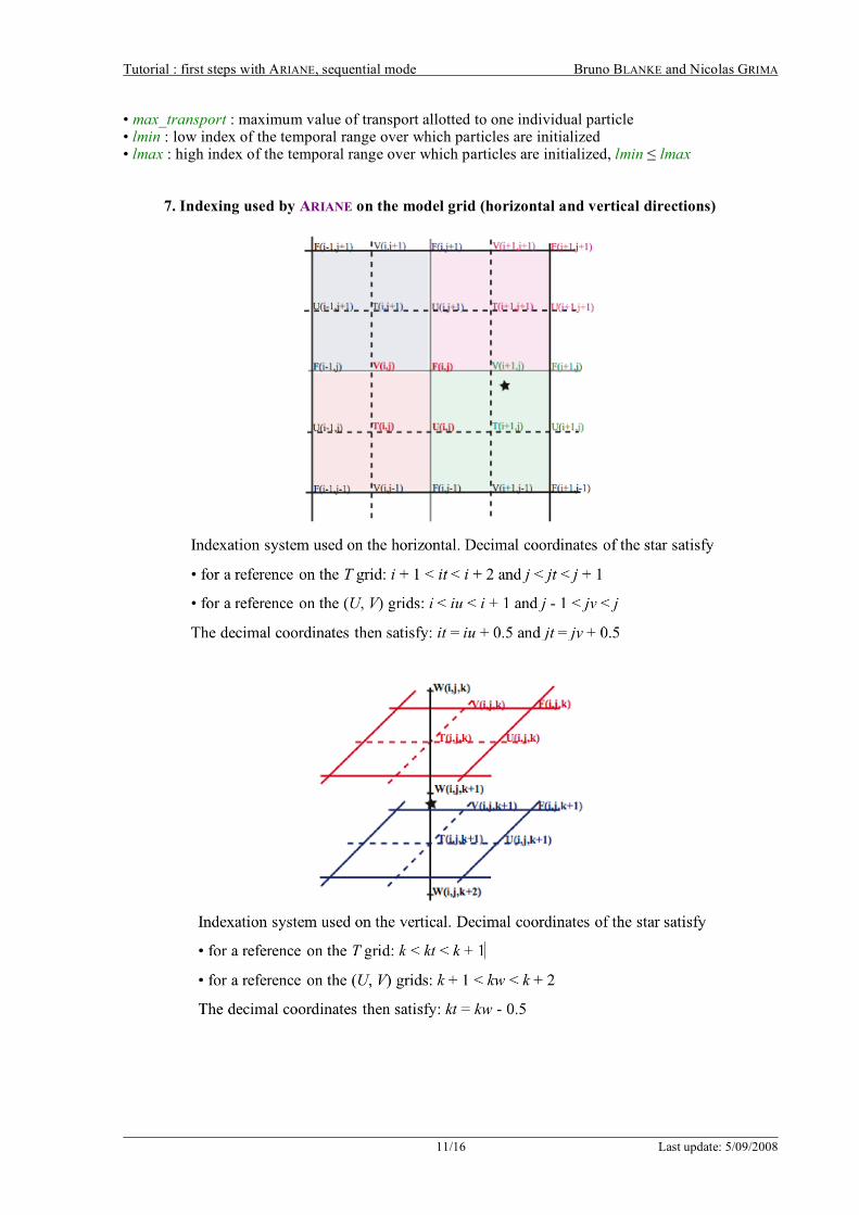
I can visualize the organization of the U, V, W and T grids and the way to specify accurately a position on the velocity grid by referring myself to the graphs given at the end of section 5.

For positioning particles in time, an integer value corresponds to the center of the period covered by the corresponding time sample on file. Thus, if I have a monthly velocity speed (lmt = 12), a value 4.0 of the time parameter will initialize the particle at the date of April 15, 12:00. I would specify the date of December 31, 24:00, by using the value 12.5 (or 0.5).

1 I am careful not to leave truncated lined at the end of this file. There must be as many lines as initial positions. 2 This fifth parameter appears only for consistency with the format used in the quantitative experiments run with ARIANE. I

initialize it with an arbitrary value (typically 1.0), while being conscious that it will be ignored in qualitative calculations. 3 I do not initialize my particles exactly on the corner of a temperature gridcell, as the velocity is imperfectly defined there.

An initial positioning at the center of T gridpoints proves often judicious. To do that, I must use “half-integer” values (as 8.5) for each of the three parameters of the spatial positioning.


4/16 Last update: 5/09/2008

I can require constant-layer calculations for trajectories (i.e., without using the vertical component of the velocity) by putting a minus sign (-) before the initial vertical index.

In the ARIANE item of the namelist file, I specify that I want a qualitative experiment (full

monitoring of the successive positions of one or several particles, mode = 'qualitative'), for the study of their fate (forback = 'forward').

I do not use for the moment the possibility to restart from the results of a former experiment, and my initial positions are actually provided by file initial_positions.txt. Therefore I use the NOBIN code for bin.

I make sure that the number of trajectories I want to integrate does not exceed the value given by nmax. If needed, I increase the value of this parameter in namelist.

In the QUALITATIVE item of namelist, I need to fill out the time parameters describing the Lagrangian trajectories. I understand that this set of parameters is completely independent of (and disconnected from) the Eulerian parameters ntfic and tunit previously introduced in item ARIANE of the same file. After having defined for delta_t a convenient unit of time in seconds (for example 86400, for a day), I indicate the interval (frequency) I want between two successive position outputs4 on file for my particles (for example 10, for 10 days), and the total number of positions (nb_output) I want (for example 20 if I want the calculation of a 200-day trajectory). The product of the three parameters nb_output×frequency×delta_t gives the length of the trajectory in seconds.

I am to check that the integration length and the initial time index of the particles put up with the duration of the velocity time series that is actually read on file (and that is controlled, among other parameters, by lmt). Should I ask for a too long integration ARIANE will loop on the provided archive, unless this goes against the value of parameter maxcycles that is specified in namelist.

If I want to include the surface mask of the model (“land” gridpoints) in the ASCII output of the trajectory file, I use .TRUE. for key mask.

I run the program simply by typing ariane in the directory where I edited both files

namelist and initial_positions.txt. In order to analyze later the numerous messages of ARIANE standard output, I can redirect the output on file : ariane > ariane_output.txt

The result (“land” gridpoints and successive positions for particles) is in the ASCII file

traj.txt, where one line represents one position. The outcome of this Lagrangian experiment is taken back in the ariane_trajectories_qualitative.nc netCDF file with a binary format that respects the full accuracy of the internal calculations done in machine.

On each line of file traj.txt, I find the following information : index of the particle (0 stands for “land” gridpoints), x, y, z, time (in number of tcyc 5), T, S, σn.

I note that I have given initial coordinates to ARIANE on the model grid (mesh indices) but that the result of the experiment (traj.txt or ariane_trajectories_qualitative.nc) is directly expressed in the form of geographical and time coordinates (longitude, latitude, depth, age). As already specified, ages are expressed in number of parameter tcyc.

Everything works perfectly for the time being, and I choose to use the result of this first run to

test backward calculations. I start from the final position obtained at the end of the first experiment and I check if I succeed

to go back to the initial positions that were previously defined. I use for this new experiment the binary archive (full precision) of the final positions of the first

experiment. I copy file ariane_trajectories_qualitative.nc in another directory (for example

EXPER02) under the name ariane_initial.nc, possibly with a symbolic link to minimize disk usage, and I specify now the code 'bin' 6 instead of 'nobin' in the new namelist that I make sure to create in this new directory (simply by copying the first namelist). In this same file, I use 4 As ARIANE uses analytical calculations, this parameter does not affect the precision of the calculated trajectories. It is only a

parameter used for graphical precision purposes. 5 I can obtain a trajectory shorter than what I explicitly asked in the namelist if ever my particle is intercepted by ARIANE

on the edges (or at the surface) of the domain covered by the grid. 6 As I use the code BIN, the content of initial_positions.txt will be ignored: ARIANE will use the positions given

in intial.bin to start the calculation of the trajectories.


5/16 Last update: 5/09/2008

from now on a 'backward' direction of integration and I give the value 'final' to key init_final since I want to use the final positions of the first experiment as my new initial positions.

As I did not modify the FORTRAN code itself, I do not need to compile or install the binaries again, and I just type ariane in the directory where I just edited the new namelist and created ariane_initial.nc.

With a precision within my machine accuracy, I check that I find the same trajectory than

previously in traj.txt, but calculated backward : I fell on my feet! The BIN code in the namelist file forces restarting of all the particles present in

ariane_initial.nc. I can go on with a qualitative experiment starting from only a subset of these positions by using code 'subbin' instead of 'bin', and by listing, line after line, in an additional file named subset.txt, the indices of the only particles that I want to re-use7.

b) Quantitative experiments Since the qualitative experiments do not pose specific problems, I will now run a quantitative

experiment, in a new directory where I can copy the namelist file of my first successful qualitative experiment.

I activate the mode 'quantitative' in namelist, instead of 'qualitative', and I go

back to a 'forward' direction. I reactivate the 'nobin' code as my quantitative experiment will not use the result of a former

experiment. Time parameters in item QUALITATIVE of the namelist file control only the sampling of

the individual trajectories in the qualitative mode and will no longer be used by ARIANE. Consequently, I ignore them and I jump directly to the max_transport key of item QUANTITATIVE : it defines the precision of the quantitative experiments.

In order to limit the computing time, I start with the lowest possible precision by increasing artificially the maximum value of transport (max_transport, in m3/s) that may be associated with each particle. I use 109 as recommended. I will be able to refine my results thereafter by reducing this value.

The usual purpose of a quantitative experiment is the evaluation of the mass transport

established between an “initial” section of the domain and final interception sections8. For this reason, I must define a closed sub-volume within my domain of study, whose simplest formulation is that of a right-angled parallelepiped. More complex formulations can describe a larger variety of shapes.

Such sections are defined in the form of segments, forming vertical planes in the Ox (i = it1 to it2, j = jt0, k = kt1 to kt2) or Oy (i = it0, j = jt1 to jt2, k = kt1 to kt2) directions, or horizontal planes (i = it1 to it2, j = jt1 to jt2, k = kt0).

I build my sections with such segments, I assign to each section a sequence number (with 1 matching the section where the particles will be initialized), and I use a proper orientation9 for each of them (to inform ARIANE about the localization of the interior and the outside of the domain of study). I copy this information in file sections.txt.

I can use the tools provided in the ARIANE package (mkseg0 and mkseg) to obtain a first and

reliable definition of segments. I run first program mkseg0 to write (in file segrid, with an ASCII format) the land-ocean

mask at the model surface. I open the output file (segrid) with a suitable text editor (nedit is recommended here), so as

to visualize in a convenient way the integrality of the domain. I define by hand the sections I want to use, by replacing “ocean” (and solely “ocean”) gridpoints

by an appropriate section index. I make sure that the segments related to a same section have a length 7 In a SUBBIN configuration, I must introduce the indices in subset.txt by order ascending (using for example the UNIX

command sort –n). Otherwise I am likely to see ARIANE blunder badly in the selection of my particles. 8 The initial section is also used as a section of interception, in order to diagnose any possible recirculation. 9 A correct orientation of the segments is imperative for the initial section, and optional (but recommended) for the other

(final) sections. The convention for orientation (a positive or negative sign of it0, jt0 or kt0) is described in the comments given in file sections.txt.


6/16 Last update: 5/09/2008

larger or equal to 2 gridpoints. I am careful to define a closed domain, limited by section indices or “land” gridpoints.

I end this step by putting a “@” sign on an “ocean” gridpoint located inside the active domain. This hot spot will allow mkseg to differentiate the interior and the outside of my active domain, and to give a correct orientation to each segment. Here follows an example of a successful edition of file segrid :

-----------------------############# #----------------------######--##### ##1111111111111111111111#------##### ###---------------------3--------### ###---------------------3--------### ###---------------------3--------### ###---------------------3--------### ###---------------------333333333### ###------------------------------### ###------------------------------### ####---------@-------------------### ####-----------------------------### #####----------------------------### ######222222222222222222222222222### ######---------------------------### #######--------------------------###

I run mkseg to obtain the segments that compose my sections. With the previous example I get

the following lines : Total number of segments : 4 1 3 24 -14 -14 1 31 "1section" 2 7 33 3 3 1 31 "2section" 3 25 33 -9 -9 1 31 "3section" 3 -25 -25 9 13 1 31 "3section"

In the event of mistakes while editing segrid, some error messages might be returned, and, in

file segrid, a star “*” should appear in the immediate vicinity of a problem. I must redo the construction of this file by correcting it the best I can.

With determination, I end up with a clean output (no more error messages), and I copy the result

(namely the coordinates of the segments calculated by mkseg) in file sections.txt, within the same directory. I can check that a file named region_limits now exists in this same directory.

I introduce an explicit label for each section (instead of 1section, 2section, …), and possibly add a “lid” as an additional horizontal section of control in order to intercept the particles feeling a vague desire to evaporate in the atmosphere. For this last section, I vary i from 1 to imt, j from 1 to jmt and I choose kt1 and kt2 equal to kt0 = 0.

Then I pause to consider the appropriate calendar for the Lagrangian experiment. I must understand that ARIANE is going to define initial positions for particles over section 1, as

defined in file sections.txt, all over the velocity time series read on archived model files. Then, trajectories will be integrated with time till they are intercepted by the control sections I also defined in sections.txt, or till a given “hydrological” criterion is checked. If the archive on file is not long enough to allow for the required calculations, ARIANE will loop on the archive, except if the value used for maxcycles opposes it. In this latter case, a particle that is not intercepted within the time allowed will be considered as lost!

Therefore, it is suitable to make sure that the duration of the trajectories does not exceed a maximum value carefully thought out. One way to reach this objective is the introduction of a “hydrographical” interception criterion that concerns in fact the final time indices of the particles. In


7/16 Last update: 5/09/2008

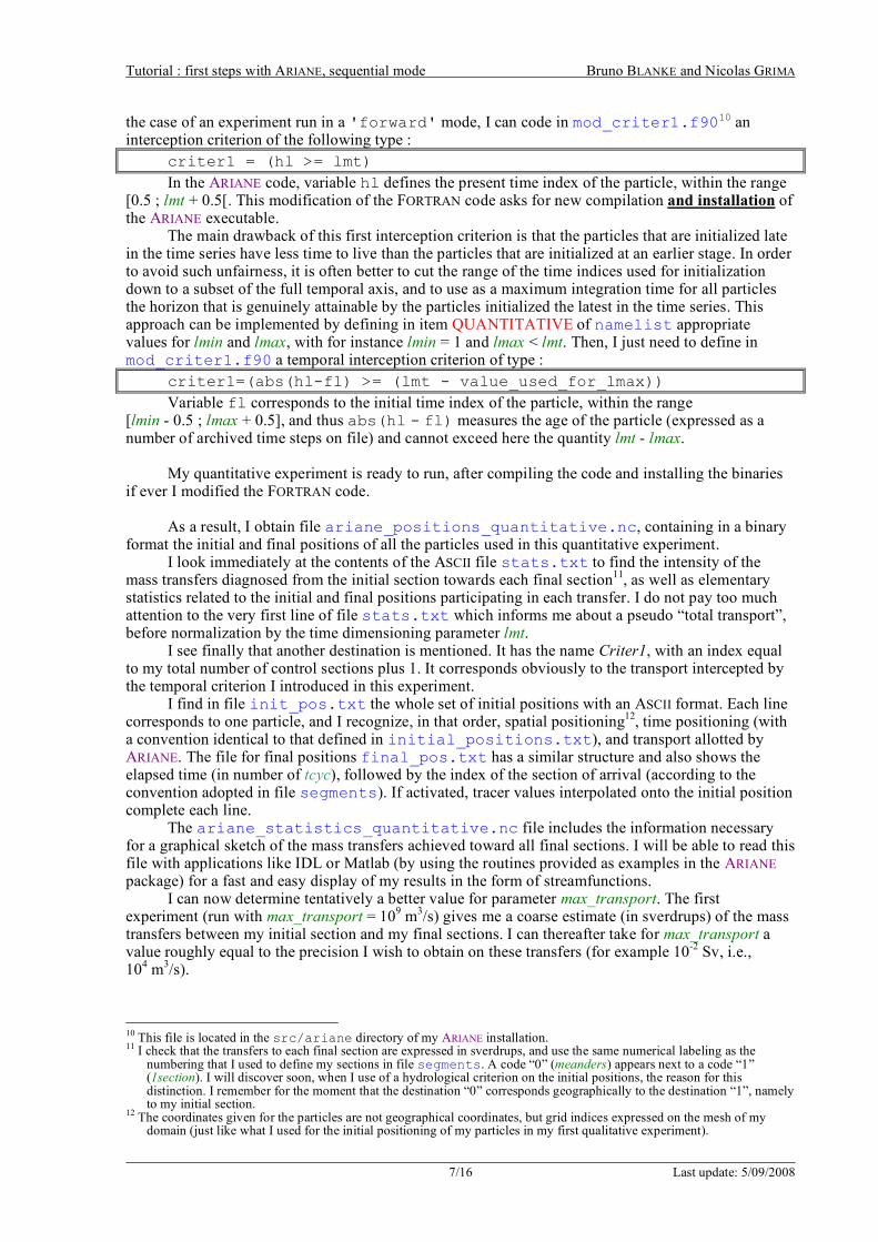
the case of an experiment run in a 'forward' mode, I can code in mod_criter1.f9010 an interception criterion of the following type :

criter1 = (hl >= lmt)

In the ARIANE code, variable hl defines the present time index of the particle, within the range [0.5 ; lmt + 0.5[. This modification of the FORTRAN code asks for new compilation and installation of the ARIANE executable.

The main drawback of this first interception criterion is that the particles that are initialized late in the time series have less time to live than the particles that are initialized at an earlier stage. In order to avoid such unfairness, it is often better to cut the range of the time indices used for initialization down to a subset of the full temporal axis, and to use as a maximum integration time for all particles the horizon that is genuinely attainable by the particles initialized the latest in the time series. This approach can be implemented by defining in item QUANTITATIVE of namelist appropriate values for lmin and lmax, with for instance lmin = 1 and lmax < lmt. Then, I just need to define in mod_criter1.f90 a temporal interception criterion of type :

criter1=(abs(hl-fl) >= (lmt - value_used_for_lmax))

Variable fl corresponds to the initial time index of the particle, within the range [lmin - 0.5 ; lmax + 0.5], and thus abs(hl - fl) measures the age of the particle (expressed as a number of archived time steps on file) and cannot exceed here the quantity lmt - lmax.

My quantitative experiment is ready to run, after compiling the code and installing the binaries

if ever I modified the FORTRAN code. As a result, I obtain file ariane_positions_quantitative.nc, containing in a binary

format the initial and final positions of all the particles used in this quantitative experiment. I look immediately at the contents of the ASCII file stats.txt to find the intensity of the

mass transfers diagnosed from the initial section towards each final section11, as well as elementary statistics related to the initial and final positions participating in each transfer. I do not pay too much attention to the very first line of file stats.txt which informs me about a pseudo “total transport”, before normalization by the time dimensioning parameter lmt.

I see finally that another destination is mentioned. It has the name Criter1, with an index equal to my total number of control sections plus 1. It corresponds obviously to the transport intercepted by the temporal criterion I introduced in this experiment.

I find in file init_pos.txt the whole set of initial positions with an ASCII format. Each line corresponds to one particle, and I recognize, in that order, spatial positioning12, time positioning (with a convention identical to that defined in initial_positions.txt), and transport allotted by ARIANE. The file for final positions final_pos.txt has a similar structure and also shows the elapsed time (in number of tcyc), followed by the index of the section of arrival (according to the convention adopted in file segments). If activated, tracer values interpolated onto the initial position complete each line.

The ariane_statistics_quantitative.nc file includes the information necessary for a graphical sketch of the mass transfers achieved toward all final sections. I will be able to read this file with applications like IDL or Matlab (by using the routines provided as examples in the ARIANE package) for a fast and easy display of my results in the form of streamfunctions.

I can now determine tentatively a better value for parameter max_transport. The first experiment (run with max_transport = 109 m3/s) gives me a coarse estimate (in sverdrups) of the mass transfers between my initial section and my final sections. I can thereafter take for max_transport a value roughly equal to the precision I wish to obtain on these transfers (for example 10-2 Sv, i.e., 104 m3/s).

10 This file is located in the src/ariane directory of my ARIANE installation. 11 I check that the transfers to each final section are expressed in sverdrups, and use the same numerical labeling as the

numbering that I used to define my sections in file segments. A code “0” (meanders) appears next to a code “1” (1section). I will discover soon, when I use of a hydrological criterion on the initial positions, the reason for this distinction. I remember for the moment that the destination “0” corresponds geographically to the destination “1”, namely to my initial section.

12 The coordinates given for the particles are not geographical coordinates, but grid indices expressed on the mesh of my domain (just like what I used for the initial positioning of my particles in my first qualitative experiment).


8/16 Last update: 5/09/2008

I decide to run a new quantitative experiment, and activate new functionalities in ARIANE. I take the same domain of study, but I choose to use a different section as a starting section.

Since mkseg already did a clean work, I only need to edit file sections.txt to allocate number 1 (initial section) to the segments defining the new section I want to use for the initialization of the particles (for example numbered 3 in the former experiment) and to give number 3 to the former initial section (simple swap of indices).

I also choose to refine the definition of the initial positions by asking ARIANE to keep only the

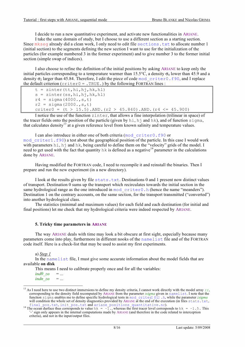
initial particles corresponding to a temperature warmer than 15.5°C, a density σ4 lower than 45.9 and a density σ2 larger than 45.84. Therefore, I edit the piece of code mod_criter0.f90, and I replace the default criterion (criter0 = .TRUE.) by the following FORTRAN lines :

t = zinter(tt,hi,hj,hk,hl) s = zinter(ss,hi,hj,hk,hl) r4 = sigma(4000.,s,t) r2 = sigma(2000.,s,t) criter0 = (t > 15.5).AND.(r2 > 45.840).AND.(r4 <= 45.900)

I notice the use of the function zinter, that allows a fine interpolation (trilinear in space) of the tracer fields onto the position of the particle (given by hi, hj and hk), and of function sigma, that calculates density13 at a given reference level from known salinity and temperature values.

I can also introduce in either one of both criteria (mod_criter0.f90 or

mod_criter1.f90) a test about the geographical position of the particle. In this case I would work with parameters hi, hj and hk, being careful to define them on the “velocity” grids of the model. I need to get used with the fact that quantity hk is defined as a negative14 parameter in the calculations done by ARIANE.

Having modified the FORTRAN code, I need to recompile it and reinstall the binaries. Then I

prepare and run the new experiment (in a new directory). I look at the results given by file stats.txt. Destinations 0 and 1 present now distinct values

of transport. Destination 0 sums up the transport which recirculates towards the initial section in the same hydrological range as the one introduced in mod_criter0.h (hence the name “meanders”). Destination 1 on the contrary accounts, on the same section, for the transport transmitted (“converted”) into another hydrological class.

The statistics (minimal and maximum values) for each field and each destination (for initial and final positions) let me check that my hydrological criteria were indeed respected by ARIANE.

5. Tricky time parameters in ARIANE The way ARIANE deals with time may look a bit obscure at first sight, especially because many

parameters come into play, furthermore in different nooks of the namelist file and of the FORTRAN code itself. Here is a check-list that may be used to assist my first experiments.

a) Step 1 In the namelist file, I must give some accurate information about the model fields that are

available on disk This means I need to calibrate properly once and for all the variables: ind0_zo = ... indn_zo = ...

13 As I need here to use two distinct immersions to define my density criteria, I cannot work directly with the model array rr,

corresponding to the density field recomputed by ARIANE from the parameter zsigma given in namelist. I note that the function sigma enables me to define specific hydrological tests in mod_criter[01].h, while the parameter zsigma will condition the whole set of density diagnostics provided by ARIANE at the end of the execution (in files stats.txt, final_pos.txt, init_pos.txt and ariane_positions_quantitative.nc).

14 The ocean durface thus corresponds to value hk = –1., whereas the first tracer level corresponds to hk = –1.5. This ’-’ sign only appears in the internal computations made by ARIANE (and therefore in the code related to interception criteria), and not in the input/output files.


9/16 Last update: 5/09/2008

maxsize_zo = ... (and the same for variables V, W, T, S, R) a) Step 2 In the namelist file, I must give some appropriate information about the maximum number

of time steps that I will actually use for my Lagrangian experiments This means that I need to calibrate properly the variable: lmt15 = ... Of course, lmt must not exceed the total number of time steps available on disk, as implicitly

determined by the parameters initialized in Step 1. It can be smaller if I do not plan to work over the full range of instants stored on disk. It is essential for me to understand that the first instant of the lmt-long time series, usable for Lagrangian experiments, will correspond to the first instant of the first file indexed by Step 1. The last (lmt) instant will be determined automatically by ARIANE, after successful reading of successive model values.

c) Step 3 For qualitative Lagrangian experiments applied to real-time archived data, I must not ask for

calculation times that would go past the lmt-long time series. Therefore, I need to be cautious when adjusting the following parameters in the namelist file :

delta_t = ... frequency = ... nb_output = ... I should always have: delta_t × frequency × nb_output < tunit × ntfic × lmt Furthermore, if I use initial time indices (fl, 4th column in file initial_positions.txt)

larger than 0.5 (knowing that 0.5 is the very start of the lmt-long time series: [0.5 ; lmt + 0.5[), the criterion must be even more restrictive. I should in fact check that16 :

delta_t × frequency × nb_output < tunit × ntfic × (lmt + 0.5 - max(fl)) For quantitative Lagrangian experiments applied to real-time archived data, I do not want the

initial positions to be distributed over the full [0.5 ; lmt + 0.5[ axis. Instead, I am likely to group them at the beginning of the time series (for instance over a 1-year-long period) and to integrate all of them for a maximum time equal to or shorter than the remaining period (typically several years).

Then, I need to specify in the namelist file the initialization window [lmin - 0.5; lmax + 0.5[, with lmin >= 1 and lmax <= lmt :

lmin = ... lmax = ... At the same time, I should implement an interception based on time, by editing the FORTRAN

code related to “criter1” (file mod_criter1.f90) and by specifying an interception test that could be for instance17 :

criter1=(abs(hl-fl) >= (lmt - value_used_for_lmax)) 6. Summary of the keywords of the namelist file I note that more detailed information is to be found in the technical document “How to write an

Ariane namelist file ?”. I begin with the keywords of the items related to the fields that need to be read on disk, keeping

in mind that the first instant of the first file identified for each model variable will be the first instant of the time series loaded by ARIANE. These blocs are :

ZONALCRT MERIDCRT

15 For ROMS applications, I would use variable time instead of lmt 16 For backward calculations, I must use a similar inequality to check that the length of the Lagrangian integration does not

extend beyond the data available on disk 17 for backward calculations, the strategy is equivalent but the initialization window must be defined toward the end of the

lmt-long time series


10/16 Last update: 5/09/2008

VERTICRT (if I am to read vertical velocity on file) TEMPERAT (if I need this tracer) SALINITY (if and only if item TEMPERAT is filled in) DENSITY (if item TEMPERAT is present and if I wand to read density on file) Then, in the ARIANE item, I specify the sampling period of the data readable on disk, the time

basis to be used to express ages, the sequential mode, as well as my choice about activation (or not) of diagnoses related to tracers : • tunit : appropriate time unit expressed in seconds • ntfic : sampling period of the archived velocity (in number of tunit) • tcyc : appropriate time basis (in seconds) for age display by ARIANE • key_sequential : .TRUE. if I cannot load all 4D fields in central memory • key_alltracers : .TRUE. if tracers are required

If I use the “sequential” mode, I need to document item SEQUENTIAL :

• maxcycles : maximum number of loops over the archived model fields Then I fill in all the fields of item MESH (or GRDROMS) related to the model grid. I continue by specifying in item OPAPARAM (or ROMSPARAM) the space dimensions of the

fields to be read on file, the number of time steps to read (it will define the length of the time series over which Lagrangian calculations will be done) and some specificities of the mesh : • imt or xi_rho : number of points along the i direction for the OPA/NEMO (or ROMS) fields • jmt or eta_rho : number of points along the j direction • kmt or s_w : number of points along the k direction • lmt or time : number of time steps of the time series over which Lagrangian calculations will be run • key_periodic : .TRUE. if there is i periodicity in OPA/NEMO • key_jfold : .TRUE. if there is j folding in OPA/NEMO • pivot : to be defined if key_jfold is .TRUE., with ‘T’ or ‘F’ according to the type of pivotal point • key_partialsteps : if “partial steps” were implemented in OPA/NEMO

Still in item OPAPARAM, I must specify the way vertical velocity and density are to be

managed : • key_computew : if .FALSE. item VERTICRT must be filled in • key_sigma : if .FALSE. item DENSITY must be filled in

The remaining parameters depend closely on the specificities of the Lagrangian experiment

under consideration. In item ARIANE I still have to define : • mode : 'qualitative' or 'quantitative' • forback : 'backward' or 'forward' mode • bin : 'nobin' (standard), 'bin' (restart) or 'SUBBIN' (restart on subset) mode • init_final : 'final' or 'init', if 'bin' or 'subbin' modes are defined • nmax : maximum number of particles usable by ARIANE • zsigma : if key_sigma is .TRUE. reference depth for calculation of density

In the case of a “qualitative” experiment, I must fill in item QUALITATIVE :

• delta_t : practical time unit (in seconds) for the Lagrangian storage • frequency : spacing between two outputs (as a number of delta_t) • nb_output : number of outputs • key_region : .TRUE. only if a subregion for Lagrangian calculations is to be read in central memory • mask : .TRUE. if the land-ocean mask must be present in the ASCII file created for the trajectories

In the case of a “quantitative” experiment, I must fill in item QUANTITATIVE :

• key_2dquant : .TRUE. if trajectories must be calculated without vertical displacement • key_eco : .TRUE. for more economical (but less comprehensive) calculations • key_reducmem : .TRUE. for a selective reading of model fields over the area of interest • key_unitm3 : .TRUE. for transports expressed in m3/s rather than in Sv


11/16 Last update: 5/09/2008

• max_transport : maximum value of transport allotted to one individual particle • lmin : low index of the temporal range over which particles are initialized • lmax : high index of the temporal range over which particles are initialized, lmin ≤ lmax

7. Indexing used by ARIANE on the model grid (horizontal and vertical directions)


12/16 Last update: 5/09/2008

8. Additional information about our Lagrangian analysis approach a) Introduction The ARIANE utility developed at the Laboratoire de Physique des Océans (LPO, Brest, France)

makes possible the description of the dynamics simulated by an Ocean General Circulation Model (OGCM) as OPA from a Lagrangian point of view.

Such diagnostics are based on the calculation of multiple trajectories in the modeled velocity field, with an advection scheme particularly fitted to the three-dimensional nature of the oceanic circulation [Blanke and Raynaud, 1997] and to an effective description of a water mass from the particles which form it [Döös, 1995].

Within the framework of the European program TRACMASS18 (June 1998 - May 2001), these analyses were applied to various classes of OGCM (an isopycnic and three z-coordinate models), over distinct domains (the Mediterranean Sea and the global ocean), with various spatial resolutions.

One key issue in the Lagrangian tracing of ocean water masses is the characteristic times of large scale advection. The Lagrangian trajectories must be integrated for sufficiently a long time to describe the full range of the movements at a basin or global scale. This means several hundreds, even thousands of years, whereas direct OGCM simulations seldom exceed a few tens of years because of CPU time constraints or drift problems.

One way to by-pass this difficulty is the development of diagnostics run from the archive of the model fields (and associated tracers), with repeated loops over the archived period (usually a climatological year). This offline approach is tempting because of its flexibility, but it raises nevertheless two major questions : • What is the impact of unresolved frequencies (in the archived output) on the subsequent offline trajectory calculations and other Lagrangian diagnostics? • Can one be satisfied with such an approach in the case of an archive limited to a fraction of a simulation presenting signs of drift (i.e. an imperfect adjustment to the surface forcing) or with strong interannual variability?

This last point could be addressed by our TRACMASS collaborators and does not concern this presentation. The contribution of LPO to the methodological section of the same TRACMASS project allowed us to study the first point in a model with a coarse horizontal resolution (the ORCA2 version of the OPA model, with a 2° zonal resolution), and without drift (as it was run a in robust-diagnostic mode) [Valdivieso Da Costa and Blanke, 2003]. Within this framework of climatological modeling at coarse space resolution, we could show that a monthly archive of the velocity field (that was sampling appropriately the seasonality of the various internal and surface forcing functions) proved to be necessary for the development of reliable Lagrangian analyses.

b) Advantages of a C grid The equations of the OPA model are discretized on a C-type grid [Arakawa, 1972]. This mesh

system proves is ideal for the analytical calculation of successive streamline segments [Blanke and Raynaud, 1997] from a time sampled velocity field (with period ∆T).

This Lagrangian integration scheme respects the local conservation of mass and thus defines a judicious tool to carry out water mass tracing. The latter technique lies on the insemination of a given water mass (considered on a geographical section) by tens or hundreds of thousands of individual particles [Döös, 1995 ; Blanke and Raynaud, 1997], and by assigning to each of them an infinitesimal fraction of the incoming transport. For a selected set of final destinations (other geographical sections, or the satisfaction of a hydrological criterion), infinitesimal transports can be combined and allow the evaluation of directional transports (i.e., the water flow between two selected sections).

c) Individual trajectories The analytical calculation of streamlines on the model grid, for successive ∆T periods over

which the velocity speed is assumed to remain constant, offers several advantages. This method for computing trajectories is both fast and accurate : it only calculates positions on the edge of individual gridcells, and it respects fully the local three-dimensional non-divergence of the flow. The method is flexible too, and backward integrations can be performed to track the origin of a given current, insofar as calculations do not involve diffusive phenomena.

18 “Tracing the water masses of the North Atlantic and the Mediterranean”


13/16 Last update: 5/09/2008

By making the assumption of a linear variation of each component of the velocity speed along each corresponding direction, elementary relations are written to describe the trajectory equations along the three axes. The integration in time of these equations allows to bind each co-ordinate (x, y, or z) to time inside each model gridcell. Crossing times in each direction are evaluated independently by imposing as a possible final position each of the six sides of the gridcell. The minimum of these estimates gives the exact crossing time, and allows the accurate calculation of the final position on the exit side.

d) Detailed calculations [Blanke and Raynaud, 1997] Usual ways to compute trajectories from GCM outputs involve first the interpolation of the

three-dimensional velocity at the location of a given particle, then the advection of this particle in the direction of the current. Such methods require accurate interpolation and advection schemes to minimize possible cumulative errors in the computation of the trajectories. In the present study, we take advantage of the C grid used for discretizations in the OPA model to compute analytically trajectories from model outputs. The algorithm calculates true trajectories for a given stationary velocity field through the exact computation of three-dimensional streamlines. Under the assumption of stationarity, such streamlines indeed represent trajectories of particles advected by the given velocity field. The three components of the velocity are known over the six faces of each cell. The non divergence of the velocity field then ensures continuous trajectories within this cell. We develop here some equations with the tensorial formalism used in the OPA model [Marti et al., 1992], which allows a more general approach than a simple Cartesian view, with for instance the description of a distorted grid over the sphere. Using the same notations as Marti et al. [1992], the divergence of the three-dimensional velocity field V = (U, V, W) is expressed as

∆V = b -1 [∂i(e2 e3 U) + ∂j(e1 e3 V) + ∂k(e1 e2 W)], (1) where n = i, j, or k refers to the grid index for the three axes ; n refers to the corresponding finite

difference ; e1, e2, and e3 are the scale factors (in the three directions) computed at each velocity grid point ; and b is the product e1 e2 e3 computed at the center of a given cell (“temperature” grid point). For any choice of the grid, the non-divergence of the flow now simply writes as

∂iF + ∂jG + ∂kH = 0, (2) where F, G, and H designate the transports in the three directions, with F = e2 e3 U, etc. We

assume now that the three components of the transport vary linearly between two opposite faces of one individual cell. This hypothesis respects the local three-dimensional non-divergence of the flow. It means that, within a given cell, F depends linearly on i, G depends linearly on j, and H depends linearly on k, where i, j, and k are considered as fractional within the cell (i.e., as non integer). In the cell extending from i = 0 to i = 1, one can write for instance for F

F(r) = F0 + r ∆F, (3) with r ∈ [0, 1] and F(0) = F0, and where ∆F stands for F(1) - F(0). One can also write the

equation linking position and velocity, namely dx/dt = U, for the transport dr/ds = F, (4) with s = (e1 e2 e3) -1 t and x = e1 r. With some adequate initial conditions, for example, r = 0 for

s = 0, one can combine (A.3) and (A.4) and find the time dependency of r within the considered cell r = F0 ∆F -1 [exp(∆F s) – 1]. (5a) If ∆F = 0, only the limit of (A.5a) for ∆F → 0 is to be considered r = F0 s. (5b) Similar relationships are of course obtained along both other directions. Since these expressions

only apply in one individual cell, one also has to determine the time when a given particle switches to another cell, or equivalently the time when r is equal to its exit value (here r = 1). Time dependency is obtained from a different writing of (4) :

ds = F -1 dr. (6) Using (3), one obtains the following expression for ds : ds = (F ∆F) -1 dF. (7) A crossing time in the zonal direction can only be obtained if F(1) and F(0) have the same sign,

and this implies F ≠ 0 in the cell. If this condition is not verified for F, the three-dimensional non-divergence of the velocity field ensures that at least one other direction satisfies it. One can assume that this condition is checked in the zonal direction. The pseudo time s is then related to the transport F by

s = ∆F -1 ln(F / F0). (8)


14/16 Last update: 5/09/2008

The crossing time in this direction corresponds to the moment when the transport reaches the exit face value, F(1) :

∆s = ∆F -1 ln([F0 + ∆F] / F0), (9a) or, if ∆F = 0, its limit when ∆F → 0 : ∆s = 1 / F0. (9b) As previously mentioned, at least one of the three crossing times is to be defined through such a

formulation. The shortest one defines the traveling time in the considered cell. Thus, if the particle first attains the zonal extremity of the cell, its positions on the meridional and vertical axes are deduced from the equations of the trajectories using s = ∆s. Computations are done for the next cell, with a starting point equal to the exit point of the previous one, and the “age” of the particle is regularly updated summing the expressions (9) obtained for ∆s.

e) Quantitative diagnostics Quantitative results are obtained by increasing considerably the number of particles (possibly up

to several millions), following the technique developed by Döös [1995] and Blanke and Raynaud [1997]. Due to water incompressibility, one given particle with an infinitesimal section is to conserve its infinitesimal mass along its trajectory. As a current can be entirely determined by the particles that compose it, with well-defined characteristics (position, velocity, and other scalars), the transport of a given water mass can be calculated from its own particles and their associated infinitesimal transport.

For most of the quantitative diagnostics run with ARIANE, the area of each gridcell, for a given instant and with a given transport Ti, is described with particles whose Ni

3 initial positions are homogeneously distributed in space and time (with lagged departure times). The number of subdivisions along each direction, Ni, satisfies

Ti / Ni3 ≤ T0, (10)

where T0 is the prescribed maximum transport associated with a single particle. The total number of particles used to describe the water mass is the sum of the Ni’s, over the relevant grid points of the section and the total number of instants (as for instance the 12 months of a climatological year), knowing that a homogeneous space-time distribution of particles is used in each sub gridcell [Blanke et al., 1999].

The best positioning of the particles over an initial section is indeed the one that gives the highest accuracy in the computation of the transports associated with the circulation, for a reasonable number of initial positions. A measurement of the accuracy is the difference between “section to section” transports computed for a stationary velocity field with both forward and backward integrations, as both transports are virtually equal. “Constant number of particles by gridcell” and “spatially homogeneous distributions” are not satisfactory because they may use too few (many) particles to describe regions of weak (slow) currents. The best approach is the one that distributes particles so that they have the same transport, thus grouping them in regions where the velocity is the highest.

f) Lagrangian mass streamfunctions We compute trajectories for all the particles and sum algebraically the Ti on each junction of

two model gridcells, on the velocity grid points of the staggered C-grid [Arakawa 1972]. Northward and eastward movements are counted positive, while southward or westward movements are counted negative. We obtain a three-dimensional transport field that corresponds to the flow of the water mass in study, within the domain of integration of the trajectories. As one particle entering one model gridcell through one of its six faces has to leave it (by another face), the transport field exactly satisfies

∂iTx + ∂jTy + ∂kTz = 0, (11) where Tx , Ty , and Tz designate the directional flows (in sverdrups) in the three directions, and

where i, j, or k refers to the grid index for the three axes. Integrating this field along a selected direction (either the vertical, zonal, or meridional axis), we obtain a two-dimensional non-divergent field that we study by means of a streamfunction. For a vertically integrated transport or a zonally integrated transport, we define ψh and ψyz, respectively, with

∂iψh = Σk Ty

∂jψh = - Σk Tx (12a) and ∂iψyz = Σk Tz


15/16 Last update: 5/09/2008

∂jψyz = - Σk Ty (12b) and contours of ψh or ψyz provide an adequate view of the movement in projection onto the

selected plane. As contours cannot cross each other (by construction of a streamfunction), the more accurately and selectively we define the initial conditions of the particles, the more similar the contours are to actual projections of trajectories. The choice of a horizontal projection usually turns out judicious, but an additional plane of projection or plots of selected individual trajectories may be helpful in plotting the precise movement of the water mass.

g) LPO publications related to the use of ARIANE

Blanke, B., and S. Raynaud, 1997 : Kinematics of the Pacific Equatorial Undercurrent : a Eulerian and Lagrangian approach from GCM results. Journal of Physical Oceanography, 27, 1038-1053.

Blanke, B., M. Arhan, G. Madec, and S. Roche, 1999 : Warm water paths in the equatorial Atlantic as diagnosed with a general circulation model. Journal of Physical Oceanography, 29, 2753-2768.

Speich, S., B. Blanke, and G. Madec, 2001 : Warm and cold water paths of a GCM thermohaline conveyor belt. Geophysical Research Letters, 28, 311-314.

Blanke, B., S. Speich, G. Madec, and K. Döös, 2001 : A global diagnostic of interocean mass transfers. Journal of Physical Oceanography, 31, 1623-1642.

Blanke, B., M. Arhan, S. Speich, and K. Pailler, 2002 : Diagnosing and picturing the North Atlantic segment of the global conveyor belt by means of an ocean general circulation model. Journal of Physical Oceanography, 32, 1430-1451.

Blanke, B., S. Speich, G. Madec, and R. Maugé, 2002 : A global diagnostic of interior ocean ventilation, Geophysical Research Letters, 29, 10.1029/2001GL013727.

Speich S., B. Blanke, P. de Vries, K. Döös, S. Drijfhout, A. Ganachaud, and R. Marsh, 2002 : Tasman leakage : a new route in the global ocean conveyor belt. Geophysical Research Letters, 29, 10.1029/2001GL014586.

Blanke, B., M. Arhan, A. Lazar, and G. Prévost, 2002 : A Lagrangian numerical investigation of the origins and fates of the salinity maximum water in the Atlantic. Journal of Geophysical Research, 107, 3163, doi :10.1029/2002JC001318.

Izumo, T., J. Picaut, and B. Blanke, 2002 : Tropical pathways, equatorial undercurrent variability and the 1998 La Niña, Geophysical Research Letters, 29, 2080, doi :10.1029/2002GL015073.

Blanke, B., C. Roy, P. Penven, S. Speich, J. McWilliams, and G. Nelson, 2002 : Linking wind and upwelling interannual variability in a regional model of the southern Benguela. Geophysical Research Letters, 29, 2188, doi :10.1029/2002GL015718.

Rodgers, K., B. Blanke, G. Madec, O. Aumont, P. Ciais, and J.-C. Dutay, 2002 : Extratropical sources of equatorial Pacific upwelling in an OGCM. Geophysical Research Letters, 30, 1084, doi :10.1029/2002GL016003.

Valdivieso Da Costa, M., and B. Blanke, 2003 : Sensitivity of trajectory calculations to the time resolution of the velocity data from a non eddy-resolving OGCM. Sous presse dans Ocean Modelling.

Blanke, B., S. Speich, A. Bentamy, C. Roy, and B. Sow, 2005 : Modeling the structure and variability of the southern Benguela upwelling using QuikSCAT wind forcing. Journal of Geophysical Research, 110, C07018, doi :10.1029/2004JC002529.

Friocourt, Y., S. Drijfhout, B. Blanke, and S. Speich, 2005 : Export of water masses from the Drake Passage to the Atlantic, Indian and Pacific Oceans : A Lagrangian model analysis. Journal of Physical Oceanography, 35, 1206-1222.

Radenac, M.-H., Y. Dandonneau, and B. Blanke, 2005 : Displacements and transformations of nitrate-rich and nitrate-poor water masses in the tropical Pacific during the 1997 El Niño. Ocean Dynamics, 55, 34–46.

Blanke, B., M. Arhan, and S. Speich, 2006 : Salinity changes along the upper limb of the Atlantic thermohaline circulation. Geophysical Research Letters, 33, L06609, doi :10.1029/2005GL024938.

Doglioli, A.M., M. Veneziani, B. Blanke, S. Speich, and A. Griffa, 2006. A Lagrangian analysis of the Indian-Atlantic interocean exchange in a regional model. Geophysical Research Letters, 33, L14611, doi :10.1029/2006GL026498.

Speich S., J. Lutjeharms, P. Penven, and B. Blanke, 2006 : The role of bathymetry in Agulhas Current configuration and behaviour. Geophysical Research Letters, 33, L23611, doi :10.1029/2006GL027157.

Durand, F., D. Shankar, C. de Boyer Montegut, S. S. C. Shenoi, B. Blanke, and G. Madec, 2007 : Modeling the barrier-layer formation in the South-Eastern Arabian Sea. Journal of Climate, 20, 2109-2120.

Doglioli A. M., B. Blanke, S. Speich, and G. Lapeyre, 2007 : Tracking coherent structures in a regional ocean model with wavelet analysis : Application to Cape Basin eddies. Journal of Geophysical Research, 112, C05043, doi :10.1029/2006JC003952.

Friocourt Y., B. Levier, S. Speich, B. Blanke, and S. S. Drijfhout, 2007 : A regional numerical ocean model of the circulation in the Bay of Biscay. Journal of Geophysical Research, 112, C09008, doi :10.1029/2006JC003935.

Pizzigalli C., V. Rupolo, E. Lombardi, and B. Blanke, 2007 : Seasonal Probability Dispersion Maps in the Mediterranean Sea obtained from the MFS Eulerian velocity fields. Journal of Geophysical Research, 112, C05012, doi :10.1029/2006JC003870.

Dutrieux, P., C. E. Menkes, J. Vialard, P. Flament, and B. Blanke, 2007 : Lagrangian study of tropical Instability vortices in the Atlantic. Journal of Physical Oceanography, 38, 400-417.


16/16 Last update: 5/09/2008

Iudicone D., S. Speich, G. Madec, and B. Blanke, 2008 : The global Conveyor Belt in a Southern Ocean perspective. Journal of Physical Oceanography, 38, 1401–1425.

Muller, H., B. Blanke, F. Dumas, V. Mariette, and F. Lekien, 2008 : Estimating the Lagrangian residual circulation in the Iroise Sea. In press in Journal of Marine Systems.

h) Cited references

Arakawa, A., 1972 : Design of the UCLA general circulation model. Numerical simulation of weather and climate. Tech. Rep. 7, Dept. of Meteorology, University of California, Los Angeles, 116 pp.

Döös, K., 1995 : Inter-ocean exchange of water masses. J. Geophys. Res., 100, 13499–13514. Marti, O., G. Madec, and P. Delecluse, 1992 : Comment on “Net diffusivity in ocean general circulation models with

nonuniform grids” by F. L. Yin and I. Y. Fung. J. Geophys. Res., 97, 12763–12766.

Tutorial : first steps with ARIANE, sequential version ...grima/Ariane/ariane_tutorial_2.x.x... ·...

Documents

Transcript of Tutorial : first steps with ARIANE, sequential version ...grima/Ariane/ariane_tutorial_2.x.x... ·...