Tutorial: chemical reaction network theory for bothdeterministic and stochastic models

David F. Anderson∗

∗anderson@math.wisc.edu

Programming with Chemical Reaction Networks: MathematicalFoundations

June 9th, 2014

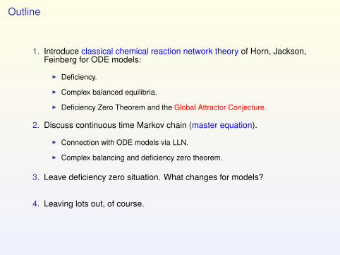
Outline

1. Introduce classical chemical reaction network theory of Horn, Jackson,Feinberg for ODE models:

I Deficiency.

I Complex balanced equilibria.

I Deficiency Zero Theorem and the Global Attractor Conjecture.

2. Discuss continuous time Markov chain (master equation).

I Connection with ODE models via LLN.

I Complex balancing and deficiency zero theorem.

3. Leave deficiency zero situation. What changes for models?

4. Leaving lots out, of course.

Main references: classical work for deterministic systems

Jeremy Gunawardena,Chemical reaction network theory for in-silico biologists,http://vcp.med.harvard.edu/papers/crnt.pdf

Martin Feinberg,Lectures on Chemical Reaction Networks,(Delivered at the Mathematics Research Center, U. of Wisconsin, 1979)http://crnt.engineering.osu.edu/LecturesOnReactionNetworks

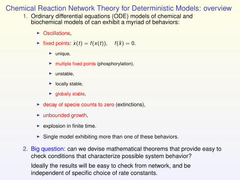
Chemical Reaction Network Theory for Deterministic Models: overview1. Ordinary differential equations (ODE) models of chemical and

biochemical models of can exhibit a myriad of behaviors:

I Oscillations,

I fixed points: x(t) = f (x(t)), f (x) = 0.

I unique,

I multiple fixed points (phosphorylation),

I unstable,

I locally stable,

I globally stable,

I decay of specie counts to zero (extinctions),

I unbounded growth,

I explosion in finite time.

I Single model exhibiting more than one of these behaviors.

2. Big question: can we devise mathematical theorems that provide easy tocheck conditions that characterize possible system behavior?

Ideally the results will be easy to check from network, and beindependent of specific choice of rate constants.

Can not cover whole field. Focus on fixed points

Question: Are there general theorems that categorize when fixed pointsexist? What about stability?

Many mathematicians would look at you funny and tell you to find anotherproblem:

I “These are highly nonlinear polynomial systems”I “Hopeless”

CRNT:I Provides several theorems about systems of nonlinear, polynomial

ODEs.

I I will focus on the results related to fixed points, deficiency theory, andthe global attractor conjecture.

I I will also branch out to stochastically modeled systems.

Key insight

The key insight of CRNT is that

I The apparent nonlinearity of the ODEs arising from mass-action kineticsconceals a great amount of linearity.

I This comes from the interplay of nonlinear, polynomial rates, and thelinear structure underlying the reaction graph.

I similar to how linearity shows up in the study of Markov chains....

I Fixed points can arise in two ways:

1. Due to the linear structure,

2. Due to an artifact of the nonlinearity.

I The deficiency measures the degree to which the second can arise.

I Deficiency of zero implies only the first kind (and lots of other things!)

A reaction network

There are:

Species: S = {A,B,C,D,E}.

Complexes: C = {A, 2B, A + C, D, B + E}.

Reactions: R = {A→ 2B, 2B → A, A + C → D, . . . }.

First danger point: Complexes mean something different to me than to manyof you!

Reaction graph

David’s model: Question: X1 = X2?

X1 + X2 → Y

Y + N → Y

X1 + Y → X1 + N

X2 + Y → X2 + N

I will write

X1 + X2 ↘Y

Y + N ↗

X1 + Y → X1 + N

X2 + Y → X2 + N

Reaction vectors

• ConsiderA + C → D

• We make the association:

A + C “=” y =

10100

, D “=” y ′ =

00010

.

• Note: each instance of the reaction

A + C → D or y → y ′

changes the state of the system by the vector:

y ′ − y =

−10−110

.

Chemical Reaction Networks: Species, Complexes, and Reactions

DefinitionA chemical reaction network, {S, C,R}, consists of:

1. Species, S := {S1, . . . ,Sd}: constituent molecules undergoing a seriesof chemical reactions.

2. Complexes, C: linear combinations of the species representing thoseused, and produced, in each reaction.

Can represent as vectors, yk , y ′k ∈ Zd≥0, representing the numbers of

molecules of each species consumed and created in the k th reaction,respectively.

3. A set of reactions, R := {yk → y ′k}, with reaction vectors y ′k − yk ∈ Zd .

Dynamics: development of ordinary differential equation (ODE) model

Let x(0) ∈ Rd≥0 be some initial concentration level, let x(t) be concentration

at time t .

Question: How is x(t) changing in time?

Let rk (t) be rate at which reaction yk → y ′k is proceeding at time t . Then,

x ′(t) =∑

k

rk (x(t), t) · (y ′k − yk ).

Usually take rk (x(t), t) to be mass-action kinetics.

Mass-action kinetics

The standard (but not only!) rate function chosen is mass-action kinetics:

Reaction rate function∅ κ1→ S1 r1(x) = κ1

S1κ2→ S2 r2(x) = κ2x1

S1 + S2κ3→ S3 r3(x) = κ3x1x2

2S1κ4→ S2 r4(x) = κ4x2

1

4S2 + 3S4 → anything r5(t) = κ5x42 x3

4

Note that for the reaction yk → y ′k ,

rk (x) = κk · xyk11 · xyk2

2 · · · xykdd = κk

d∏i=1

xykii

We define:

xyk def=

d∏i=1

xykii

(with 00 def= 1)

Chemical Reaction Systems

DefinitionA mass-action chemical reaction system is a quadruple, {S, C,R, κ}:

1. Species, S := {S1, . . . ,Sd}.

2. Complexes, C: linear combinations of the species.

3. reactions, R := {yk → y ′k}.

4. rate constants, κ : R→ R>0

The time evolution of a chemical reaction system is given by:

dxdt

=∑

k

κk xyk (y ′k − yk )

ordxdt

=∑

y→y′κy→y′x

y (y ′ − y)

Dynamics: deterministic model

Example:

Dynamics: deterministic model

Example:

A + Bκ1→ 2B (R1)

Bκ2→ A (R2)

x ′(t) = κ1 · xA(t)xB(t)[−11

]+ κ2 · xB(t)

[1−1

].

or

x ′A(t) = −κ1 · xA(t)xB(t) + κ2 · xB(t)

x ′B(t) = κ1 · xA(t)xB(t)− κ2 · xB(t)

Examples

Examples: (You should be thinking: how does he know so much?)

Board 1.

Answer

These models are weakly reversible and have a deficiency of zero.

Network reversibility conditions

DefinitionA chemical reaction network, {S, C,R}, is called weakly reversible if eachlinkage class is strongly connected.

A network is called reversible if y ′k → yk ∈ R whenever yk → y ′k ∈ R.

0 0.1 0.2 0.3 0.4 0.5 0.6 0.7 0.8 0.9 10

0.1

0.2

0.3

0.4

0.5

0.6

0.7

0.8

0.9

1

C3 C2

C1

Weakly Reversible

0 0.1 0.2 0.3 0.4 0.5 0.6 0.7 0.8 0.9 10

0.1

0.2

0.3

0.4

0.5

0.6

0.7

0.8

0.9

1

C3 C2

C1

Reversible

Deficiency

Need: linkage class and span of reaction vectors. Then, Attempt 1:

δ = n − `− s,

where

1. n = # of complexes.

2. ` = # of linkage classes.

3. s = dimension of span of reaction vectors.

Now you are probably thinking: Fiiiiine, but what does it mean? Attempt 2:

A measure of how independent reactions are.

Board 2.

But what is really going on here? Attempt 3. (Technical)

The hunt for linearity

We definef (x)

def=∑

y→y′κy→y′x

y (y ′ − y),

and will now find other functions, Y , Aκ, and Ψ for which

f (x) = Y ◦ Aκ ◦Ψ(x).

The hunt for linearity

Define the linear mapping Aκ : RC → RC by

(Aκ)ij =

κj→i for j 6= i

−∑6=j

κj→` for i = j

Example

A + Bκ1�κ2

2Bκ3�κ4

2A,

then

Aκ =

−κ1 κ2 0κ1 −(κ2 + κ3) κ4

0 κ3 −κ4

,

(Note: same for C1

κ1�κ2

C2

κ3�κ4

C3,: x = Aκx .)

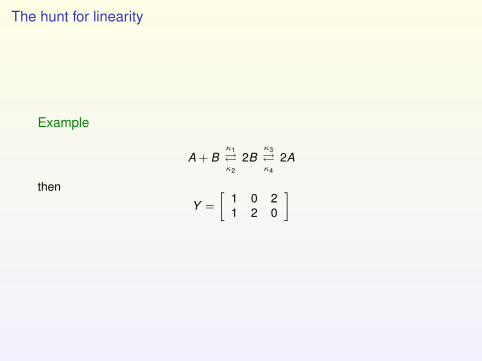
The hunt for linearity

Example

A + Bκ1�κ2

2Bκ3�κ4

2A

then

Y =

[1 0 21 2 0

]

The hunt for linearity

Example

A + Bκ1�κ2

2Bκ3�κ4

2A gives Ψ(x) =

xAxB

x2B

x2A

Now

Y (Ak (Ψ(x))) =∑

y→y′κy→y′x

y · (y ′ − y) =: f (x),

the original rate equation!

Example

General Case: Example: A + Bκ1�κ2

2Bκ3← 2A

x = f (x) = Y ◦ Aκ ◦Ψ(x) x = κ1xAxB

[−11

]+ κ2x2

B

[1−1

]+ κ3x2

A

[−22

]Ψ : Rd → RC

Ψ(x)y = xy Ψ(x) =

xAxB

x2B

x2A

Aκ : RC → RC

Aijκ =

{κj→i for j 6= i

−∑` 6=j κj→` for i = j Aκ =

−κ1 κ2 0κ1 −κ2 κ3

0 0 −κ3

Y : RC → Rd is linear:

Y (ωy ) = y Y =

[1 0 21 2 0

]

x =

[1 0 21 2 0

] −κ1 κ2 0κ1 −κ2 κ30 0 −κ3

xAxB

x2B

x2A

Deficiency: attempt 3

f (x) = Y ◦ Aκ ◦Ψ(x).

The deficiency of the model is

δ = dim(ker Y ∩ imageAκ).

You are probably thinking: Oh my, that did not help at all..... in fact, I think itmade things significantly worse.

My response: remember, we are thinking about fixed points:

f (x) = Y ◦ Aκ ◦Ψ(x) = 0

with x ∈ Rd>0. This can happen in one of two ways:

(i) Aκ(Ψ(x)) ∈ ker Y or (ii) Ψ(x) ∈ ker Aκ.

The second is the very nice condition I knew we had: all equilibria are nice orComplexed Balanced

Properties of x with Ψ(x) ∈ ker Aκ

Theorem (Horn and Jackson)Suppose that there is an x ∈ Rd

>0 for which f (x) = 0 with Aκ(Ψ(x)) = 0.Then,

1. There does not exist a c ∈ Rd>0 for which f (c) = 0 with Aκ(Ψ(c)) 6= 0.

2. The network is weakly reversible.

3. Every stoichiometric compatibility class (invariant manifold) containsprecisely one c for which Aκ(Ψ(c)) = 0.

4. Each such c is locally asymptotically stable.

Conjecture. (Global attractor conjecture)Each such c is globally asymptotically stable relative to its compatibility class.

Theorem (Deficiency Zero Theorem - Feinberg)If a chemical reaction network has a deficiency of 0 then it has a fixed point cfor which Aκ(Ψ(c)) = 0 if and only if it is weakly reversible.

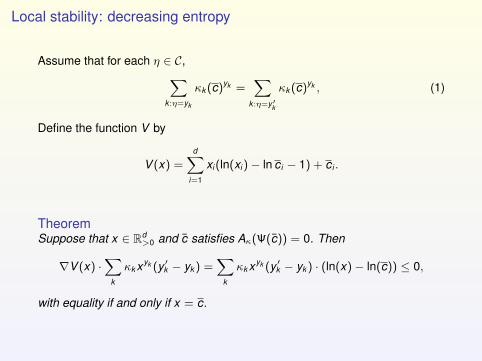
Local stability: decreasing entropy

Assume that for each η ∈ C,∑k :η=yk

κk (c)yk =∑

k :η=y′k

κk (c)yk , (1)

Define the function V by

V (x) =d∑

i=1

xi (ln(xi )− ln c i − 1) + c i .

TheoremSuppose that x ∈ Rd

>0 and c satisfies Aκ(Ψ(c)) = 0. Then

∇V (x) ·∑

k

κk xyk (y ′k − yk ) =∑

k

κk xyk (y ′k − yk ) · (ln(x)− ln(c)) ≤ 0,

with equality if and only if x = c.

Proof of local stability: decreasing entropy

Proof.First rewrite in clever way:∑

k

κk xyk (y ′k − yk ) · (ln x − ln c) =∑

k

κk (c)yk(x

c

)yk(

ln{(x

c

)y′k}− ln

{(xc

)yk})

.

Use ea(b − a) ≤ eb − ea with equality if and only if a = b∑k

κk (c)yk(x

c

)yk(

ln{(x

c

)y′k}− ln

{(xc

)yk})

≤∑

k

κk (c)yk

((xc

)y′k −(x

c

)yk)

=∑η∈C

(xc

)η ∑k :η=y′k

κk (c)yk −∑

k :η=yk

κk (c)yk

= 0

A conjectureGlobal Attractor Conjecture.For a complex-balanced system, each of the equilibria c ∈ Rd

>0 is globallyasymptotically stable relative to the interior of its compatibility class P.

Why doesn’t previous proof work? Because

V (x) 6→ ∞ as x → ∂Rd>0.

We know:

1. Holds if s ≤ 3 (Craciun, Pantea, Nazarov)

2. Holds if there is a single linkage class (Anderson).

3. Holds if network is strongly endotactic (Gopalkrishnan, Miller, Shiu).

Implied by

Persistence Conjecture. If {S, C,R} is weakly reversible, then for any κ,solution trajectories are persistent:

lim inft→∞

xi (t) > 0,

for all i .

Transition

Questions? Break? Moving on to Stochastic models:

Aim:1. Give a representation most of you will not have seen.

I Useful for analytical methods.I Useful for computational methods.

2. Use rep. to show LLN. Diffusion (Langevin) Approximation?

3. Come back to deficiency zero/weakly reversible situation.

4. Move to deficiency of 1 for both deterministic and stochastic models.

Specifying infinitesimal behavior: Random Time Changes and goingbeyond the Gillespie algorithm

Q: How do we specify model when there are low molecular counts anddynamics appears more random.

Should be

1. discrete space, since counting molecules, and

2. stochastic dynamics.

Let’s return to development of ODEs.

An ordinary differential equation is specified by describing how a functionshould vary over a small period of time

X (t + ∆t)− X (t) ≈ F (X (t))∆t

A more precise description (consider a telescoping sum)

X (t) = X (0) +

∫ t

0F (X (s))ds

Infinitesimal behavior for jump processes

We are interested in functions that are piecewise constant and random.

Changes, when they occur, won’t be small. If “reaction k ” occurs at time t ,

X (t)− X (t−) = ζk := y ′k − yk ∈ Zd

What is small? The probability of seeing a jump of a particular size.

P{X (t + ∆t)− X (t) = ζk | Ft} ≈ λζk (t)∆t

Question: Can we specify the λζk in some way that determines X?

I For the ODE, F depended on X .

I Maybe λζk should depend on X?

Simple model

For example, consider the simple system

A + B → C

where one molecule each of A and B is being converted to one of C.

Intuition for standard stochastic model:

P{reaction occurs in (t , t + ∆t ]∣∣ Ft} ≈ κXA(t)XB(t)∆t

whereI κ is a positive constant, the reaction rate constant.

I Ft is all the information pertaining to the process up through time t .

Can we specify a reasonable model satisfying this assumption?

Answer: yes, but we need Poisson processes.

Background information: The Poisson processWill view a Poisson process, Y (·), through the lens of an underlyingpoint process.

(a) Let {ei} be i.i.d. exponential random variables with parameter one.

(b) Now, put points down on a line with spacing equal to the ei :

x x x x x x x x↔e1↔e2

←→e3 · · · t

I Let Y1(t) denote the number of points hit by time t .

I In the figure above, Y1(t) = 6.

0 5 10 15 200

5

10

15

20

25

λ = 1

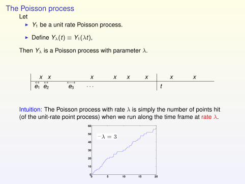
The Poisson processLet

I Y1 be a unit rate Poisson process.

I Define Yλ(t) ≡ Y1(λt),

Then Yλ is a Poisson process with parameter λ.

x x x x x x x x↔e1↔e2

←→e3 · · · t

Intuition: The Poisson process with rate λ is simply the number of points hit(of the unit-rate point process) when we run along the time frame at rate λ.

0 5 10 15 200

10

20

30

40

50

60

λ = 3

The Poisson process

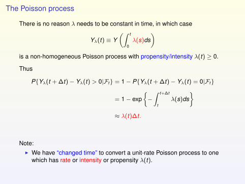
There is no reason λ needs to be constant in time, in which case

Yλ(t) ≡ Y(∫ t

0λ(s)ds

)is a non-homogeneous Poisson process with propensity/intensity λ(t) ≥ 0.

Thus

P{Yλ(t + ∆t)− Yλ(t) > 0|Ft} = 1− P{Yλ(t + ∆t)− Yλ(t) = 0|Ft}

= 1− exp{−∫ t+∆t

tλ(s)ds

}≈ λ(t)∆t .

Note:I We have “changed time” to convert a unit-rate Poisson process to one

which has rate or intensity or propensity λ(t).

Return to models of interest

Consider the simple systemA + B → C

where one molecule each of A and B is being converted to one of C.

Intuition for standard stochastic model:

P{reaction occurs in (t , t + ∆t ]∣∣Ft} ≈ κXA(t)XB(t)∆t

whereI κ is a positive constant, the reaction rate constant.

I Ft is all the information pertaining to the process up through time t .

Models of interest

A + B → C

Simple book-keeping says: if

X (t) =

XA(t)XB(t)XC(t)

gives the state at time t , then

X (t) = X (0) + R(t)

−1−11

,

whereI R(t) is the # of times the reaction has occurred by time t andI X (0) is the initial condition.

Goal: represent R(t) in terms of Poisson process.

Models of interest

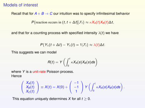
Recall that for A + B → C our intuition was to specify infinitesimal behavior

P{reaction occurs in (t , t + ∆t ]∣∣Ft} ≈ κXA(t)XB(t)∆t ,

and that for a counting process with specified intensity λ(t) we have

P{Yλ(t + ∆t)− Yλ(t) = 1|Ft} ≈ λ(t)∆t .

This suggests we can model

R(t) = Y(∫ t

0κXA(s)XB(s)ds

)where Y is a unit-rate Poisson process.Hence XA(t)

XB(t)XC(t)

≡ X (t) = X (0) +

−1−11

Y(∫ t

0κXA(s)XB(s)ds

).

This equation uniquely determines X for all t ≥ 0.

Build up model: Random time change representation of Kurtz• Now consider a network of reactions involving d chemical species,

S1, . . . ,Sd :d∑

i=1

ykiSi −→d∑

i=1

y ′kiSi

Denote reaction vector as

ζk = y ′k − yk ,

so that if reaction k occurs at time t

X (t) = X (t−) + ζk .

• The intensity (or propensity) of k th reaction is λk : Zd≥0 → R.

• By analogy with before:

X (t) = X (0) +∑

k

Rk (t)ζk ,

with

X (t) = X (0) +∑

k

Yk

(∫ t

0λk (X (s))ds

)ζk ,

Yk are independent, unit-rate Poisson processes.

Dynamics: stochastic

Example:

A + B α→ 2B (R1)

B β→ A (R2)

X (t) = X (0) + R1(t)[−11

]+ R2(t)

[1−1

].

For Markov models can take

R1(t) = Y1

(α

∫ t

0XA(s)XB(s)ds

)R2(t) = Y2

(β

∫ t

0XB(s)ds

)where Y1,Y2 are independent unit-rate Poisson processes.

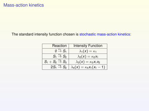
Mass-action kinetics

The standard intensity function chosen is stochastic mass-action kinetics:

Reaction Intensity Function∅ κ1→ S1 λ1(x) = κ1

S1κ2→ S2 λ2(x) = κ2x1

S1 + S2κ3→ S3 λ3(x) = κ3x1x2

2S1κ4→ S2 λ4(x) = κ4x1(x1 − 1)

Other ways to understand modelWe can also describe the model as a continuous time Markov chain withinfinitesimal generator

Af (x) =∑

k

λk (x)(f (x + ζk )− f (x)).

where ζk = y ′k − yk .

Dynkin’s formula (See Ethier and Kurtz, 1986, Ch. 1) yields

Ef (X (t))− f (X0) = E∫ t

0(Af )(X (s))ds,

Letting f (y) = 1x (y) above so that

E[f (X (t))] = P{X (t) = x} = px (t),

gives Kolmogorov’s forward equation (chemical master equation)

p′t (x) =∑

k

λ(x − ζk )pt (x − ζk )− pt (x)∑

k

λk (x)

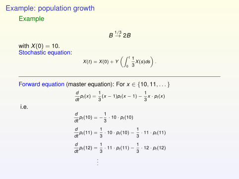
Example: population growthExample

B1/3→ 2B

with X (0) = 10.Stochastic equation:

X(t) = X(0) + Y(∫ t

0

13

X(s)ds).

Forward equation (master equation): For x ∈ {10, 11, . . . }ddt

pt (x) =13

(x − 1)pt (x − 1) −13

x · pt (x)

i.e.ddt

pt (10) = −13· 10 · pt (10)

ddt

pt (11) =13· 10 · pt (10) −

13· 11 · pt (11)

ddt

pt (12) =13· 11 · pt (11) −

13· 12 · pt (12)

...

Example: Bacterial Growth - evolution of sample paths

I Below is a plot of the solution of the deterministic system versus threedifferent realizations of the stochastic system.

0 1 2 3 4 510

20

30

40

50

60

70

Colo

ny s

ize

Time

Example: population growth - evolution of distribution

10 12 14 16 18 200

0.2

0.4

0.6

0.8

1

n

p n(0)

10 20 30 40 50 600

0.02

0.04

0.06

0.08

0.1

0.12

0.14

0.16

0.18

n

p n(1)

10 20 30 40 50 600

0.02

0.04

0.06

0.08

0.1

n

p n(2)

10 20 30 40 50 600

0.01

0.02

0.03

0.04

0.05

0.06

0.07

n

p n(3)

Dynamics: Stochastic Versus Deterministic

A + B α→ 2B (R1)

B β→ A (R2)

Stochastic equations

X (t) = X (0) + Y1

(α

∫ t

0XA(s)XB(s)ds

)[−11

]+ Y2

(β

∫ t

0XB(s)ds

)[1−1

].

Deterministic equations

x(t) = x(0) + α

∫ t

0xA(s)xB(s)ds

[−11

]+ β

∫ t

0xB(s)ds

[1−1

],

or

x(t) = αxaxb

[−11

]+ βxB

[1−1

]or

xA(t) = −αxAxB + βxB

xB(t) = αxaxB − βxB.

Dynamics: deterministic modelAssuming:

I V is a scaling parameter (volume times Avogadro’s number),

I Xi = O(V ), and X V (t) def= X (t)/V ,

I λk (X (t)) ≈ V(κk X V (t)yk

),

Then,

X V (t) ≈ 1V

X0 +∑

k

1V

Yk

(V∫ t

0κk X V (s)yk ds

)(y ′k − yk )

LLN for Yk says

1V

Yk (Vu) ≈ u

(lim

V→∞supu≤U

∣∣∣V−1Yk (Vu)− u∣∣∣ = 0, a.s.

)

so a good approximation (Gronwall, V →∞) is solution to

x(t) = x(0) +∑

k

∫ t

0κk x(s)yk ds · (y ′k − yk ),

whereuv = uv1

1 · · · uvdd ,

is standard mass-action kinetics. See Tom Kurtz’s works....

LLN: Example

I Stochastic models:

A + B2/V→ 2B (R1)

B 1→ A (R2)

with X (0) = [3V ,V ] so that [AV ,BV ] = X/V satisfies

AV (0) = 3, BV (0) = 1.

I ODE model of

A + B 2→ 2B

B 1→ A,

with x(0) = [3, 1].

LLN: Example, A + B → 2B B → A

0 1 2 3 4 50

0.5

1

1.5

2

2.5

3

3.5

4

4.5V=1

AB

0 1 2 3 4 50

0.5

1

1.5

2

2.5

3

3.5

4

4.5V=1

BA

LLN: Example, A + B → 2B B → A

0 1 2 3 4 50

0.5

1

1.5

2

2.5

3

3.5

4

4.5V=10

AB

0 1 2 3 4 50

0.5

1

1.5

2

2.5

3

3.5

4

4.5V=50

AB

LLN: Example, A + B → 2B B → A

0 1 2 3 4 50

0.5

1

1.5

2

2.5

3

3.5

4

4.5V=100

AB

0 1 2 3 4 50

0.5

1

1.5

2

2.5

3

3.5

4

4.5V=1000

AB

CRNT: Stochastic

1. We want to answer the same types of questions in stochastic setting:long term behavior from network structure.

2. No longer can search for fixed points.

3. Can look for fixed points to forward equations (master equation):stationary distribution:

Deficiency Zero Theorem - stochastic

Theorem (Anderson, Craciun, Kurtz, 2010)Suppose we have a biochemical reaction system for which the ODE modelhas a complex balanced equilibrium c (for example, the network satisfies thefollowing two conditions,

I Deficiency of zero,I weakly reversible.

)

Then, the associated stochastic model satisfies:

I There is a stationary distribution which is the product of Poissondistributions:

π(x) = Md∏

i=1

cxii

xi !, x ∈ Γ, (2)

where M is a normalizing constant.

David F. Anderson, Gheorghe Craciun, and Thomas G. Kurtz, Product-form stationarydistributions for deficiency zero chemical reaction networks, Bulletin of MathematicalBiology, Vol. 72, No. 8, 1947 - 1970, 2010.

Example: Open, first-order system

If the network is an open, first-order reaction network, then Γ = Zd≥0

π(x) = e−∑d

i=1 ci

d∏i=1

cxii

xi !=

d∏i=1

e−cicxi

i

xi !, x ∈ Zd

≥0.

where c ∈ RN>0 is the equilibrium of the associated (linear) deterministic

system.

• Thus, when in distributional equilibrium, the species numbers areindependent and have Poisson distributions. This is well known.

• However:

1. Neither the independence nor the Poisson distribution resulted from thefact that the system under consideration was a first order system.

2. Instead, both facts followed from Γ = Zd≥0.

Enzyme kinetics

Consider the possible enzyme kinetics given by

E + S � ES � E + P , E � ∅ � S

Easy to check that state space is

Γ = Z4≥0

so in distributional equilibrium

I the specie numbers are independent and

I have Poisson distributions.

Enzyme kinetics

Consider the slightly different enzyme kinetics given by

E + S � ES � E + P , E � ∅

I We see S + ES + P = N.

I In distributional equilibrium:

I E has Poisson distribution,

I S, ES, P have a multinomial distribution, and

I E is independent from S, ES, and P.

Another example

ConsiderA

α

�β

2A

I State space, assuming X0 > 0, is

Γ = {1, 2, . . . }

I ODE model satisfies

x(t) = αx(t)− βx(t)2 =⇒ c =α

β.

So, for x ∈ {1, 2, . . . }

π(x) =1

eα/β − 1· (α/β)x

x!

Another example

Example

2A � 2B.

Higher deficiency

What about the situation of δ ≥ 1?

What about higher deficiency?

Guy Shinar and Martin Feinberg, Structural Sources of Robustness inBiochemical Reaction Networks, Science, 2010.

A + B α→ 2B (R1)

B β→ A (R2)

xA(t) = −αxA(t)xB(t) + βxB(t)

xB(t) = αxA(t)xB(t)− βxB(t)

M def= xA(0) + xB(0),

Solving for equilibria:

xA = β/α,

xB = M − β/α,

Network has absolute concentration robustness in species A.

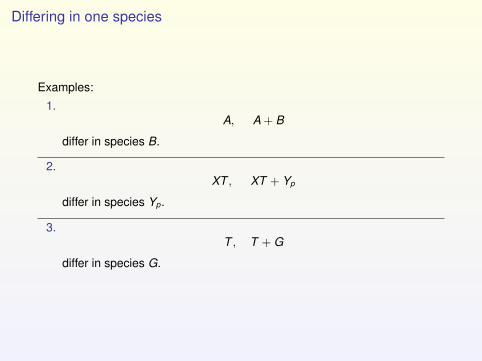
Differing in one species

Examples:

1.A, A + B

differ in species B.

2.XT , XT + Yp

differ in species Yp.

3.T , T + G

differ in species G.

Terminal and non-terminal complexes

XD X XT Xp

Xp+Y XpY X+Yp

XD+Yp XDYp XD+Y

k1

k2[ ]

k3

k4

k5

k6

k7

k8

k9

k10

k11

[ ]T

D

I The orange complexes are called terminal.

I The blue complexes are called non-terminal.

Theorems: deterministic and stochastic

Theorem (Marty Feinberg and Guy Shinar, Science, 2010 –deterministic)Consider a deterministic mass-action system that

I has a deficiency of one.I admits a positive steady state andI has two non-terminal complexes that differ only in species S,

then the system has absolute concentration robustness in S.

Theorem (Anderson, Enciso, Johnston – stochastic)Consider a reaction network satisfying the following:

I has a deficiency of one,I the deterministic model admits a positive steady state,I has two non-terminal complexes that differ only in species S,I (new) is conservative,

then with probability one there there is a last time a nonterminal reaction fires.0David F. Anderson, German Enciso, and Matthew Johnston, Stochastic analysis of biochemical

reaction networks with absolute concentration robustness, J. Royal Society Interface, Vol. 11,20130943, February 12, 2014.

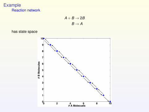
ExampleReaction network

A + B → 2B

B → A

has state space

0 2 4 6 8 100

1

2

3

4

5

6

7

8

9

10

# A Molecuels

# B

Mol

ecul

es

Example

Extinction can be rare event: quasi-stationary distribution

A + B α→ 2B

B β→ A

XA(0) + XB(0) = M,

0 2 4 6 8 100

1

2

3

4

5

6

7

8

9

10

# A Molecuels

# B

Mol

ecul

es

Find πQM so that for τ absorption time and x ∈ transient states,

limt→∞

Pν(X (t) = x | τ > t) = πQM (x).

SatisfiesπQ

M (x) = PπQM

(X (t) = x | τ > t).

Can show that quasi-stationary distribution for A converges to Poisson

πQM (x)→ e−(β/α) (β/α)x

x!, as M →∞.

Quasi-stationary distribution: EnvZ-OmpR signaling system

1

1Guy Shinar and Martin Feinberg, Structural Sources of Robustness in Biochemical ReactionNetworks, Science, 2010

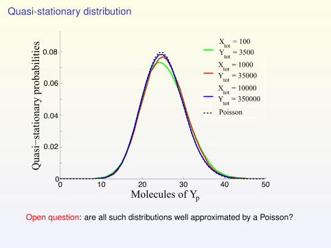
Quasi-stationary distribution

0 10 20 30 40 500

0.02

0.04

0.06

0.08

Molecules of Yp

Qua

si−s

tatio

nary

pro

babi

litie

s Xtot = 100Ytot = 3500

Xtot = 1000Ytot = 35000

Xtot = 10000Ytot = 350000

Poisson

Open question: are all such distributions well approximated by a Poisson?

Precise statement

Need a more precise statement:

There is an extinction event ⇐⇒ there will be a last time the

non-terminal complexes “fire”.

A + B α→ 2B (R1)

B β→ A (R2)

How to prove: an example

A + B α→ 2B (R1)

B β→ A (R2)

2A � B + C. (R3)

I Note |C| = 6, ` = 3, s = 2 =⇒ δ = 1.I w = (1, 1, 1) is conservation relation.

Flavor of proof

Ideas:I Decompose x = f (x) = Y ◦ Aκ ◦Ψ(x) into linear/nonlinear portions.

I Use deficiency assumption to understand the basis of ker(YAκ).

I Consider “reduced network” and prove result holds on that model.

I How?I Assume result does not hold, and that there is a recurrent state where there

should not be.

I Use stochastic equation

X(t) = X(0) +∑

k

Yk

(∫ t

0λk (X(s))ds

)(y ′k − yk ),

with a useful set of stopping times + limit theorem to construct an element inker(YAκ) which is impossible.

Flavor of proofI Can use that the deficiency of model is one to characterize basis of

kernel of YAκ : RC → RS .I

ker(YAκ) = span{c, b1, . . . , bT},

I The terms {b1, . . . , bT} have support on terminal complexes. Recall: ATκ

is the infinitesimal generator for the CTMC on network of complexes.

I The term c has support on *all* complexes.

I Now consider reduced model. I.e.

A + Bκ1→ 2B

Bκ2→ A

2Aκ3�κ4

B + C.

becomes

Bκ2→ A

2Aκ3�κ4

B + C.

flavor of proofOnly work with A + B – reduced network. Call it {S, C,R∗}. Call process X∗.

I Suppose there is a positive recurrent state X0 which charges anon-terminal complex.

I We want to reach a contradiction (with kernel condition).

I We denote the Nth return time to X0 as tN . It follows that we have

X∗(tN) = X∗(0)

for all N so that

X∗(tN) = X∗(0) +∑

k

Yk

(κi

∫ tN

0(X∗(s))yk ds

)(y ′k − yk ) = X∗(0), (3)

and so ∑k

Yk

(κi

∫ tN

0(X∗(s))yk ds

)(y ′k − yk ) = 0, (4)

I Relatively easy to show that for each yk∫ tN

0(X∗(s))yk ds →∞, as N →∞,

flavor of proof∑

k

Yk

(κi

∫ tN

0(X∗(s))yk ds

)(y ′k − yk ) = 0,

and ∫ tN

0(X∗(s))yk ds →∞, as N →∞,

I multiplying and dividing by appropriate terms,

0 =∑

k

κk

[1

κk∫ tN

0 (X∗(s))yk dsYk

(κk

∫ tN

0(X∗(s))yk ds

)×

1tN

∫ tN

0(X∗(s))yk ds

](y ′k−yk ).

I We have

limN→∞

1tN

∫ tN

0(X∗(s))yk ds =

∑X∈I

πI(X)Xyk , (5)

I Define the vector Gπ ∈ RC via

[Gπ]y :=∑X∈I

πI(X)Xy , (6)

for y ∈ C, and note that [Gπ]y > 0 for all remaining y .I Can then argue that [Gπ] is in the kernel of Y ◦ Aκ, which it can not be

(contradiction). �

May be useful to this community

Can characterize how will go to the boundary. Board 2.5.5.

Open question: how does deficiency relate to computation?

That is the story. Thanks!

Main References:

Jeremy Gunawardena,Chemical reaction network theory for in-silico biologists,http://vcp.med.harvard.edu/papers/crnt.pdf

Martin Feinberg,Lectures on Chemical Reaction Networks,(Delivered at the Mathematics Research Center, U. of Wisconsin, 1979)http://crnt.engineering.osu.edu/LecturesOnReactionNetworks

Other references:1. Guy Shinar and Martin Feinberg, Structural Sources of Robustness in

Biochemical Reaction Networks, Science, 2010.

2. David F. Anderson, German Enciso, and Matthew Johnston, Stochastic analysisof biochemical reaction networks with absolute concentration robustness, J. RoyalSociety Interface, Vol. 11, 20130943, February 12, 2014.

3. David F. Anderson, Gheorghe Craciun, Thomas G. Kurtz, Product-form stationarydistributions for deficiency zero chemical reaction networks, Bulletin ofMathematical Biology, Vol. 72, No. 8, 1947 - 1970, 2010.