Tutorial AMPL - Part I...OptIntro 5/16 AMPL AMPL: A Mathematical Programming Language I The user...
33
OptIntro 1 / 16 Tutorial AMPL Part I Eduardo Camponogara Department of Automation and Systems Engineering Federal University of Santa Catarina October 2016
Transcript of Tutorial AMPL - Part I...OptIntro 5/16 AMPL AMPL: A Mathematical Programming Language I The user...

OptIntro 1 / 16
Tutorial AMPLPart I
Eduardo Camponogara
Department of Automation and Systems EngineeringFederal University of Santa Catarina
October 2016

OptIntro 2 / 16
Summary
Introduction
AMPL
Examples

OptIntro 3 / 16
Introduction
Algebraic Modeling Languages
Definition:
I They are high-level programming languages with which onecan specify and solve optimization problems.
Properties:
I These languages do not solve the problems directly, but ratherinvoke algorithms (solvers) to obtain a solution.
I Some languages have the advantage of having a syntax similarto the mathematical notation used to describe optimizationproblems.
Examples:
I GAMS, AMPL, Pyomo, CMPL, MPL, PuLP, . . .

OptIntro 4 / 16
Introduction
Algebraic Modeling Languages
Basic Structure:
Interpretadorda linguagem
de modelagem
Solver 1
Solver 2
Solver 3
Interface deUsuário
.
.
.
Banco dedados
Tabelas
.
.
.

OptIntro 5 / 16
AMPL
AMPL: A Mathematical Programming Language
I The user interface is a terminal for input of command lines. Itis reached by running the command ampl.exe.
I The files contain the model, data, configurations, and otherprogramming structures that can be edited by a regular editor.
I There exists a developing interface, AMPL IDE, whichfacilitates the editing and execution of AMPL commands.

OptIntro 6 / 16
AMPL
AMPL
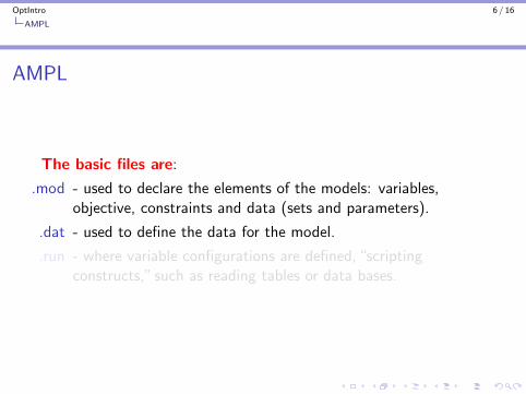
The basic files are:
.mod - used to declare the elements of the models: variables,objective, constraints and data (sets and parameters).
.dat - used to define the data for the model.
.run - where variable configurations are defined, “scriptingconstructs,” such as reading tables or data bases.
OptIntro 6 / 16
AMPL
AMPL
The basic files are:
.mod - used to declare the elements of the models: variables,objective, constraints and data (sets and parameters).
.dat - used to define the data for the model.
.run - where variable configurations are defined, “scriptingconstructs,” such as reading tables or data bases.
OptIntro 7 / 16
AMPL
AMPL
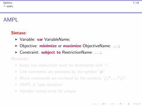
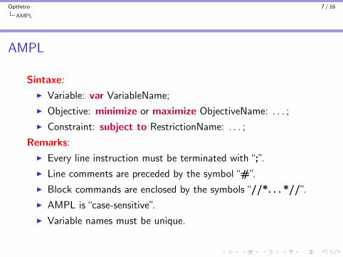
Sintaxe:
I Variable: var VariableName;
I Objective: minimize or maximize ObjectiveName: . . . ;
I Constraint: subject to RestrictionName: . . . ;
Remarks:
I Every line instruction must be terminated with “;”.
I Line comments are preceded by the symbol “#”.
I Block commands are enclosed by the symbols “//*. . . *//”.
I AMPL is “case-sensitive”.
I Variable names must be unique.
OptIntro 7 / 16
AMPL
AMPL
Sintaxe:
I Variable: var VariableName;
I Objective: minimize or maximize ObjectiveName: . . . ;
I Constraint: subject to RestrictionName: . . . ;
Remarks:
I Every line instruction must be terminated with “;”.
I Line comments are preceded by the symbol “#”.
I Block commands are enclosed by the symbols “//*. . . *//”.
I AMPL is “case-sensitive”.
I Variable names must be unique.
OptIntro 8 / 16
Examples
AMPL – Example 1
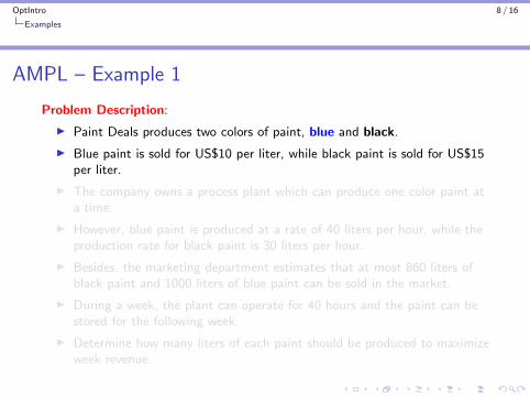
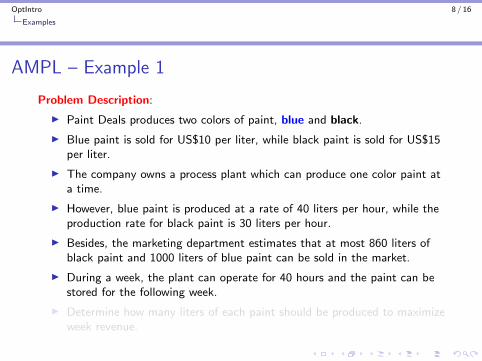
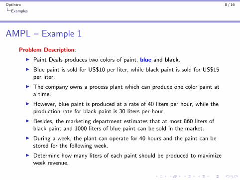
Problem Description:
I Paint Deals produces two colors of paint, blue and black.
I Blue paint is sold for US$10 per liter, while black paint is sold for US$15per liter.
I The company owns a process plant which can produce one color paint ata time.
I However, blue paint is produced at a rate of 40 liters per hour, while theproduction rate for black paint is 30 liters per hour.
I Besides, the marketing department estimates that at most 860 liters ofblack paint and 1000 liters of blue paint can be sold in the market.
I During a week, the plant can operate for 40 hours and the paint can bestored for the following week.
I Determine how many liters of each paint should be produced to maximizeweek revenue.

OptIntro 8 / 16
Examples
AMPL – Example 1
Problem Description:
I Paint Deals produces two colors of paint, blue and black.
I Blue paint is sold for US$10 per liter, while black paint is sold for US$15per liter.
I The company owns a process plant which can produce one color paint ata time.
I However, blue paint is produced at a rate of 40 liters per hour, while theproduction rate for black paint is 30 liters per hour.
I Besides, the marketing department estimates that at most 860 liters ofblack paint and 1000 liters of blue paint can be sold in the market.
I During a week, the plant can operate for 40 hours and the paint can bestored for the following week.
I Determine how many liters of each paint should be produced to maximizeweek revenue.

OptIntro 9 / 16
Examples
AMPL – Example 1
Mathematical Programming Model:
max 10 · BluePaint + 15 · BlackPaint (1)
s.t. : (1
40) · BluePaint + (
1
30) · BlackPaint ≤ 40 (2)
0 ≤ BluePaint ≤ 1000 (3)
0 ≤ BlackPaint ≤ 860 (4)
OptIntro 10 / 16
Examples
AMPL – Example 1
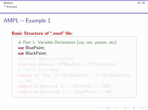
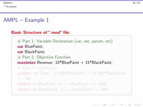
Basic Structure of “.mod” file:
# Part 1: Variable Declaration (var, set, param, etc)var BluePaint;var BlackPaint;# Part 2: Objective Functionmaximize Revenue: 10*BluePaint + 15*BlackPaint;# Part 3: Constraintssubject to Time: (1/40)*BluePaint + (1/30)*BlackPaint<= 40;subject to BlueLimit: 0 <= BluePaint <= 1000;subject to BlackLimit: 0 <= BlackPaint <= 860;
OptIntro 10 / 16
Examples
AMPL – Example 1
Basic Structure of “.mod” file:
# Part 1: Variable Declaration (var, set, param, etc)var BluePaint;var BlackPaint;# Part 2: Objective Functionmaximize Revenue: 10*BluePaint + 15*BlackPaint;# Part 3: Constraintssubject to Time: (1/40)*BluePaint + (1/30)*BlackPaint<= 40;subject to BlueLimit: 0 <= BluePaint <= 1000;subject to BlackLimit: 0 <= BlackPaint <= 860;
OptIntro 11 / 16
Examples
AMPL – Example 1
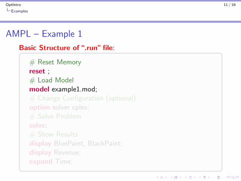
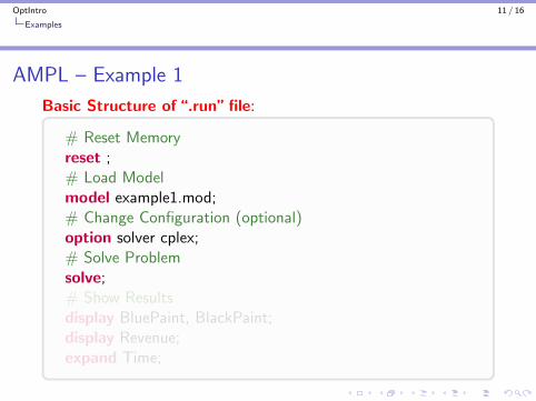
Basic Structure of “.run” file:
# Reset Memoryreset ;# Load Modelmodel example1.mod;# Change Configuration (optional)option solver cplex;# Solve Problemsolve;# Show Resultsdisplay BluePaint, BlackPaint;display Revenue;expand Time;
OptIntro 11 / 16
Examples
AMPL – Example 1
Basic Structure of “.run” file:
# Reset Memoryreset ;# Load Modelmodel example1.mod;# Change Configuration (optional)option solver cplex;# Solve Problemsolve;# Show Resultsdisplay BluePaint, BlackPaint;display Revenue;expand Time;

OptIntro 11 / 16
Examples
AMPL – Example 1
Basic Structure of “.run” file:
# Reset Memoryreset ;# Load Modelmodel example1.mod;# Change Configuration (optional)option solver cplex;# Solve Problemsolve;# Show Resultsdisplay BluePaint, BlackPaint;display Revenue;expand Time;
OptIntro 12 / 16
Examples
AMPL – Example 1
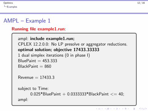
Running file example1.run:
ampl: include example1.run;CPLEX 12.2.0.0: No LP presolve or aggregator reductions.optimal solution; objective 17433.333331 dual simplex iterations (0 in phase I)BluePaint = 453.333BlackPaint = 860
Revenue = 17433.3
subject to Time:0.025*BluePaint + 0.0333333*BlackPaint <= 40;
ampl:

OptIntro 13 / 16
Examples
AMPL – Example 2Problem Description - MPC:
I AMPL is used to model a model-based predictive control problem(MPC).
I We consider a linear discrete-time system with state xk and an inputvariable uk .
I The prediction horizon is N = 4, with system dynamics given bya = 0.8104 and b = 0.2076, xinit = 0.4884.
I The cost imposes a quadratic penalty on state and control signals,leading to an optimization problem:
minN∑
k=1
(xk+1)2 +N∑
k=1
(uk)2
subject to: xk+1 = axk + buk , k = 1, . . . ,N
x1 = xinit

OptIntro 14 / 16
Examples
AMPL – Example 2
I Complete the AMPL model in example2.mod.
# Parte 1: Variable Declaration (var, set, param, etc)param a = 0.8104;param b = 0.2076;param N = 4;param Xinit = 0.4884;var x{k in 1..N+1};var u{k in 1..N};# Part 2: Objective Functionminimize Cost: sum{k in 1..N}(x[k+1]ˆ2) + ...;
I Create a file example2.run and obtain the values uk
OptIntro 15 / 16
Examples
AMPL – Example 2
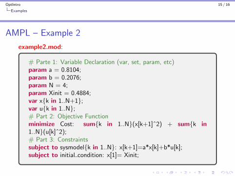
example2.mod:
# Parte 1: Variable Declaration (var, set, param, etc)param a = 0.8104;param b = 0.2076;param N = 4;param Xinit = 0.4884;var x{k in 1..N+1};var u{k in 1..N};# Part 2: Objective Functionminimize Cost: sum{k in 1..N}(x[k+1]ˆ2) + sum{k in1..N}(u[k]ˆ2);# Part 3: Constraintssubject to sysmodel{k in 1..N}: x[k+1]=a*x[k]+b*u[k];subject to initial condition: x[1]= Xinit;

OptIntro 16 / 16
Examples
Fundamentals
I Thank you for attending this lecture!!!