Tutorial 04 - Tsinghua...

MOMAP

Tutorial 04 Transport Calculation

Version 2.0 September, 2019

MOMAP Tutorial 04

Version 2.0 edited by:

Dr. Qikai Li

Dr. Yingli Niu

Ms. Lihui Yan

Released by Hongzhiwei Technology (Shanghai) Co., Ltd

and Z.G. Shuai Group

The information in this document applies to version 2.0 of MOMAP

MOMAP Tutorial - Transport Calculation

Interest in charge-carrier drift mobilities in naphthalene single crystal has been stimulated by the

discovery that the electron mobilities in the b and c' directions are independent of temperature down to about

100 K, below which they increase markedly. This increase is consistent with a transition from hopping to band

transport expected from general principles.

Here we use naphthalene single crystal as an example to show how to calculate the charge-carrier

mobilities by using the MOMAP Transport sub-package.

The basic steps involved in the calculations are as follows:

1. Prepare crystal file

2. Prepare momap.inp

3. Do transport calculations

Contents

Transport Calculation ................................................................................................................................................................1

Prepare crystal file .............................................................................................................................................................1

Prepare momap.inp ..........................................................................................................................................................2

Do Transport calculations................................................................................................................................................5

File and directory structure ....................................................................................................................................6

Transfer Integral Calculations ................................................................................................................................8

Reorganization Energy Calculations ....................................................................................................................8

Collect Transfer Integrals ........................................................................................................................................8

Analyze Reorganization Energies .........................................................................................................................8

Monte Carlo (MC) simulations ...............................................................................................................................8

Calculate Random Walk Mobilities .......................................................................................................................9

Gather data ............................................................................................................................................................. 11

1

Transport Calculations

Prepare Crystal File

First prepare the naphthalene single crystal file, in either mol or cif format, however, the cif format is prefered

as it contains the lattice information. Once the crystal file is obtained, we create a directory naphthalene as

working directory.

The naphthalene input file (naphthalene.cif) is as follows:

data_naphthalene

_audit_creation_date 2019-05-20

_audit_creation_method 'Materials Studio' _symmetry_space_group_name_H-M 'P1'

_symmetry_Int_Tables_number 1

_symmetry_cell_setting triclinic

loop_

_symmetry_equiv_pos_as_xyz

x,y,z

_cell_length_a 8.0980

_cell_length_b 5.9530

_cell_length_c 8.6520

_cell_angle_alpha 90.0000

_cell_angle_beta 124.4000

_cell_angle_gamma 90.0000

loop_

_atom_site_label

_atom_site_type_symbol

_atom_site_fract_x

_atom_site_fract_y

_atom_site_fract_z

_atom_site_U_iso_or_equiv

_atom_site_adp_type

_atom_site_occupancy

C1 C 0.082321 0.018562 0.328357 0.00000 Uiso 1.00

C2 C 0.112956 0.163833 0.222892 0.00000 Uiso 1.00

C3 C 0.047989 0.105174 0.037135 0.00000 Uiso 1.00

C4 C 0.076558 0.251823 -0.075824 0.00000 Uiso 1.00

C5 C -0.013196 -0.190207 0.254606 0.00000 Uiso 1.00

H6 H 0.124192 0.058895 0.455393 0.00000 Uiso 1.00

H7 H 0.178710 0.305594 0.271107 0.00000 Uiso 1.00

H8 H 0.141804 0.390694 -0.023603 0.00000 Uiso 1.00

H9 H -0.033302 -0.295196 0.331298 0.00000 Uiso 1.00

C10 C -0.047989 -0.105174 -0.037135 0.00000 Uiso 1.00

C11 C -0.112956 -0.163833 -0.222892 0.00000 Uiso 1.00

……

C28 C 0.547989 0.394826 0.037135 0.00000 Uiso 1.00

C29 C 0.612956 0.336167 0.222892 0.00000 Uiso 1.00

C30 C 0.582321 0.481438 0.328357 0.00000 Uiso 1.00

C31 C 0.576558 0.248177 -0.075824 0.00000 Uiso 1.00

C32 C 0.486804 0.690207 0.254606 0.00000 Uiso 1.00

H33 H 0.624192 0.441105 0.455393 0.00000 Uiso 1.00

H34 H 0.678710 0.194406 0.271107 0.00000 Uiso 1.00

H35 H 0.641804 0.109306 -0.023603 0.00000 Uiso 1.00

H36 H 0.466698 0.795196 0.331298 0.00000 Uiso 1.00

2

Fig. 1 Naphthalene unit cell

It is clear that the cif file is an output of Materials Studio with space group of ‘P1’，currently MOMAP

Transport program can support all space groups, not restricted only to space group ‘P1’. With a cif file, we

have all the crystal structure parameters in hand, as shown above.

Prepare momap.inp

Now we have prepared our crystal file, however, before we can run the MOMAP Transport calculations,

we have to prepare the momap.inp file, a control file for MOMAP package.

There exist quite a few of control parameters for momap.inp, however, all the parameters have their

default values if we do not set them. To make life easy, we have written a program called

transport_geninp.exe to generate the momap.inp for the MOMAP transport calculations.

Before we begin to generate the momap.inp, we would better setup our environment settings, as these

settings rarely change in a specific computing cluster environment. The typical environment settings are as

follows (you can put them in ~/.bashrc, for example):

These are the initial values that will be entered into our momap.inp if we run the

transport_geninp.exe, we can change them later on with an editor. The currently supported scheduling

systems include PBS, SLURM, LSF and LOCAL, these are the scheduling systems in frequent use. The LOCAL

means the jobs are run in a local machine, it can be of great help for a linux box without job scheduling

system, for example. If needed, more scheduling systems can be added.

export MOMAP_JOB_SCHED=slurm

export MOMAP_JOB_QUEUE=X12C

export MOMAP_QC_EXE=g09

export MOMAP_QC_PPN=12

export MOMAP_MODULE_QC=gaussian/g09.e01

3

If the computing cluster is installed with environment module, the last two lines can be added, but we

can change the contents according to our specific situation.

If our quantum calculation (QC) engine is of the Gaussian g16, we need to change the third line to g16,

and the fifth line to g16.b01, for example.

Once the MOMAP environments are set, we can use our transport_geninp.exe to generate

momap.inp, all the MOMAP Transport programs have a help option, either -h or --help, for example, in

case transport_geninp.exe, we have:

If option -config is used, then we can designate our output control file, the default file is momap.inp if this

option is not specified.

If option -cif is used, then cif crystal parameter will be used in momap.inp, it will automatically search for

the first found cif file in the current directory if it exists.

If option -mol is used, then mol molecule parameter will be used in momap.inp, again it will automatically

search for the mol files in the current directory.

If option -module is used, then it will activate module parameter output.

If option -terse is used, then it will generate a terse momap.inp, while the other parameters using the

default values.

If option -verbose is used, then it will generate a verbose momap.inp, almost all the parameters will be

entered into the momap.inp. Thus, we can tune the parameters as needed.

These options can be used in combination, as shown in the last line.

If we run the transport_geninp.exe without any options, it will generate a momap.inp like the following:

[test1]$ transport_geninp.exe --help

*******************************************************************

* MOMAP Transport Calculation Utility *

* Zhigang Shuai Group, Dep. of Chem., Tsinghua Univ., Beijing *

*******************************************************************

Transport Input Generation

Usage: transport_geninp.exe [opts]

-config momap.inp : set config file, default to momap.inp

-cif : use cif file as molecule input (default)

-mol : use mol file as molecule input

-module : set to use environment module flag

-terse : generate terse momap.inp (default)

-verbose : generate verbose momap.inp

e.g.: transport_geninp.exe

transport_geninp.exe -config momap.inp

transport_geninp.exe -verbose

transport_geninp.exe -cif

transport_geninp.exe -mol

transport_geninp.exe -module

transport_geninp.exe -config momap.inp -verbose

4

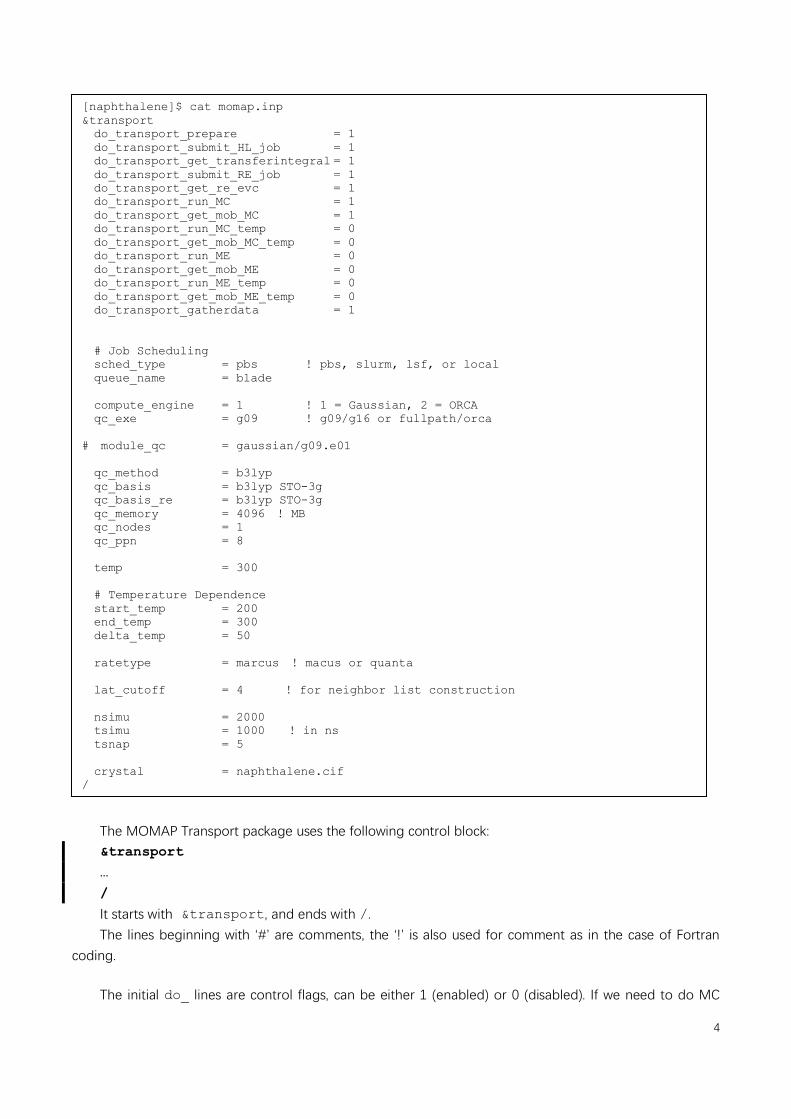
The MOMAP Transport package uses the following control block:

&transport

…

/

It starts with &transport, and ends with /.

The lines beginning with ‘#’ are comments, the ‘!’ is also used for comment as in the case of Fortran

coding.

The initial do_ lines are control flags, can be either 1 (enabled) or 0 (disabled). If we need to do MC

[naphthalene]$ cat momap.inp

&transport

do_transport_prepare = 1

do_transport_submit_HL_job = 1

do_transport_get_transferintegral = 1

do_transport_submit_RE_job = 1

do_transport_get_re_evc = 1

do_transport_run_MC = 1

do_transport_get_mob_MC = 1

do_transport_run_MC_temp = 0

do_transport_get_mob_MC_temp = 0

do_transport_run_ME = 0

do_transport_get_mob_ME = 0

do_transport_run_ME_temp = 0

do_transport_get_mob_ME_temp = 0

do_transport_gatherdata = 1

# Job Scheduling

sched_type = pbs ! pbs, slurm, lsf, or local

queue_name = blade

compute_engine = 1 ! 1 = Gaussian, 2 = ORCA

qc_exe = g09 ! g09/g16 or fullpath/orca

# module_qc = gaussian/g09.e01

qc_method = b3lyp

qc_basis = b3lyp STO-3g

qc_basis_re = b3lyp STO-3g

qc_memory = 4096 ! MB

qc_nodes = 1

qc_ppn = 8

temp = 300

# Temperature Dependence

start_temp = 200

end_temp = 300

delta_temp = 50

ratetype = marcus ! macus or quanta

lat_cutoff = 4 ! for neighbor list construction

nsimu = 2000

tsimu = 1000 ! in ns

tsnap = 5

crystal = naphthalene.cif

/

5

calculations, we simply set them to 1 accordingly.

With the generated momap.inp, we can do some fine tunings for our specific case, for example, we may

change queue_name value from blade to X12C, gaussian_ppn from 16 to 12.

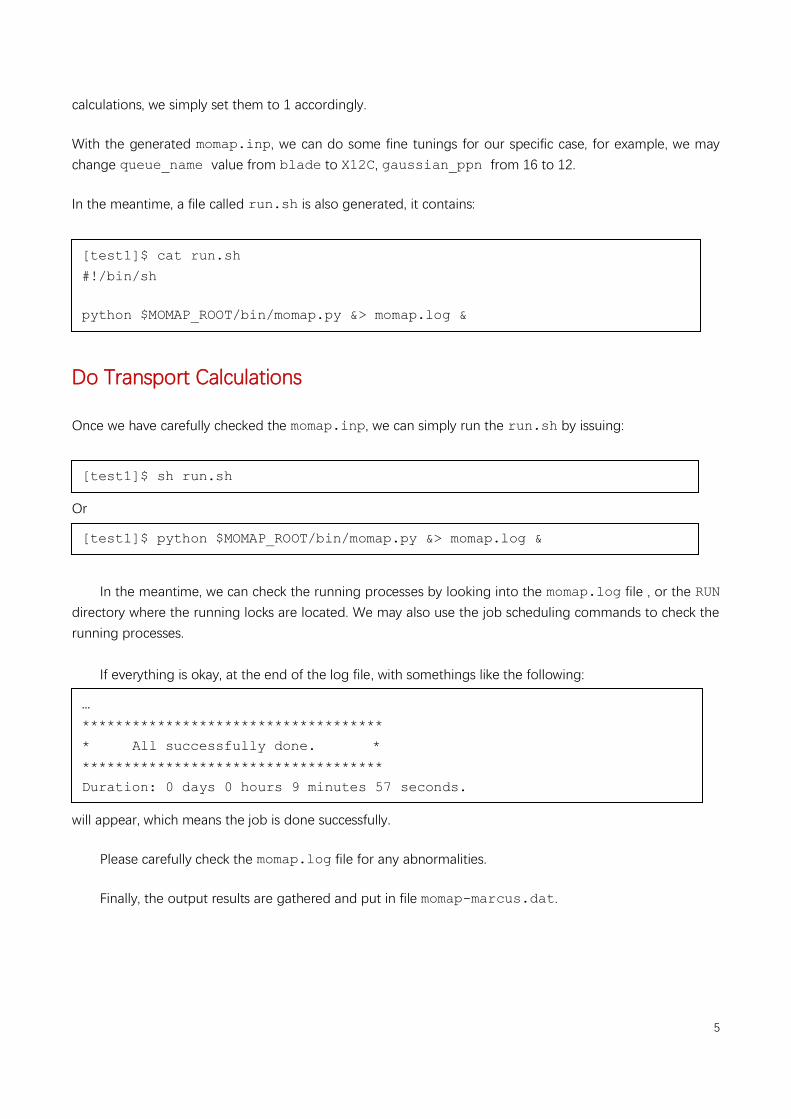
In the meantime, a file called run.sh is also generated, it contains:

Do Transport Calculations

Once we have carefully checked the momap.inp, we can simply run the run.sh by issuing:

Or

In the meantime, we can check the running processes by looking into the momap.log file , or the RUN

directory where the running locks are located. We may also use the job scheduling commands to check the

running processes.

If everything is okay, at the end of the log file, with somethings like the following:

will appear, which means the job is done successfully.

Please carefully check the momap.log file for any abnormalities.

Finally, the output results are gathered and put in file momap-marcus.dat.

[test1]$ cat run.sh

#!/bin/sh

python $MOMAP_ROOT/bin/momap.py &> momap.log &

[test1]$ sh run.sh

[test1]$ python $MOMAP_ROOT/bin/momap.py &> momap.log &

…

************************************

* All successfully done. *

************************************

Duration: 0 days 0 hours 9 minutes 57 seconds.

6

File and Directory Structure

In the process of transport calculations, quite a lot of files and directories are created. The full directory

and file tree is shown in the following pages (in Linux case, by simply run the tree command):

Cont.

[naphthalene]$ tree ./

./

├── data

│ ├── config.inp

│ ├── H.inp

│ ├── L.inp

│ ├── mol1_bonds.dat

│ ├── mol1.mol

│ ├── mol1_neighbors.cif

│ ├── mol1_trans_int_files.dat

│ ├── mol2_bonds.dat

│ ├── mol2.mol

│ ├── mol2_neighbors.cif

│ ├── mol2_trans_int_files.dat

│ ├── neighbor.dat

│ ├── supercell.cif

│ ├── unique_id_map.dat

│ └── unitcell.cif

├── evc

│ └── mol1

│ ├── elec

│ │ └── job_get_NM.pbs

│ └── hole

│ └── job_get_NM.pbs

├── HL

│ ├── 2mol-11.com

│ ├── 2mol-13.com

│ ├── 2mol-1.com

│ ├── 2mol-5.com

│ ├── 2mol-7.com

│ ├── nei_mol-11.com





│ └── uc_mol-1.com

├── jobs

│ ├── job_2mol.pbs

│ ├── job_nei_mol.pbs

│ ├── job_re-mol1-anion.pbs

│ ├── job_re-mol1-cation.pbs

│ ├── job_re-mol1-neutral.pbs

│ ├── job_transint.pbs

│ └── job_uc_mol.pbs

├── MC-marcus

│ ├── elec

│ │ ├── get_mob.pbs

│ │ ├── get_mob.py

│ │ ├── prepare-mc.py

│ │ ├── run_mc_batch.py

│ │ └── run_mc.pbs

│ └── hole

│ ├── get_mob.pbs

│ ├── get_mob.py

│ ├── prepare-mc.py

│ ├── run_mc_batch.py

│ └── run_mc.pbs

7

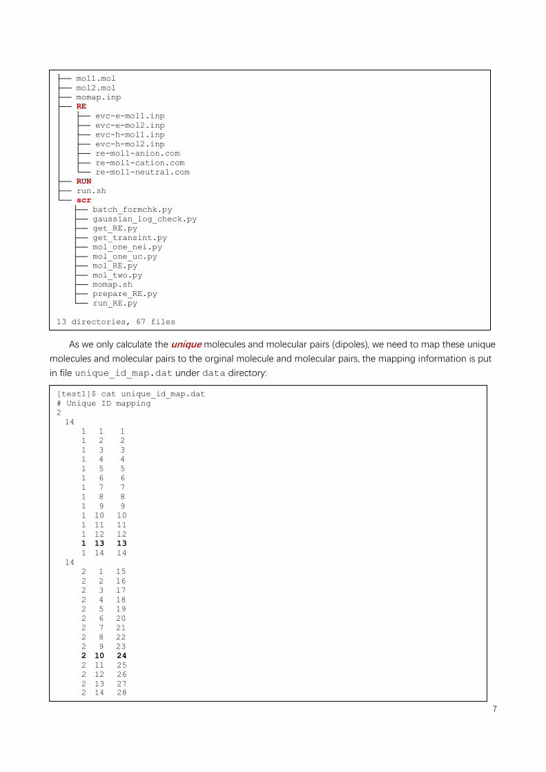
As we only calculate the unique molecules and molecular pairs (dipoles), we need to map these unique

molecules and molecular pairs to the orginal molecule and molecular pairs, the mapping information is put

in file unique_id_map.dat under data directory:

├── mol1.mol

├── mol2.mol

├── momap.inp

├── RE

│ ├── evc-e-mol1.inp

│ ├── evc-e-mol2.inp

│ ├── evc-h-mol1.inp

│ ├── evc-h-mol2.inp

│ ├── re-mol1-anion.com

│ ├── re-mol1-cation.com

│ └── re-mol1-neutral.com

├── RUN

├── run.sh

└── scr

├── batch_formchk.py

├── gaussian_log_check.py

├── get_RE.py

├── get_transint.py

├── mol_one_nei.py

├── mol_one_uc.py

├── mol_RE.py

├── mol_two.py

├── momap.sh

├── prepare_RE.py

└── run_RE.py

13 directories, 67 files

[test1]$ cat unique_id_map.dat

# Unique ID mapping

2

14

1 1 1

1 2 2

1 3 3

1 4 4

1 5 5

1 6 6

1 7 7

1 8 8

1 9 9

1 10 10

1 11 11

1 12 12

1 13 13

1 14 14

14

2 1 15

2 2 16

2 3 17

2 4 18

2 5 19

2 6 20

2 7 21

2 8 22

2 9 23

2 10 24

2 11 25

2 12 26

2 13 27

2 14 28

8

The first line is comment, the 2nd

line is the number of molecules in the central unitcell, then follows

number of neighbors for each central unitcell molecule and ID mapping data, which repeats the number of

molecules in the central unitcell. For the three-column data in the above table, the first column is the central

unitcell molecule ID, the second column is the neighbor ID for the corresponding central unitcell molecule,

and the third column is the uniformly numbered IDs for the whole central unitcell.

Thus, for example, a file 2mol-13.com has a uniform ID 13, which corresponds to central unitcell

molecule ID 1 and neighbor molecule ID 13, as show in the above list. As another example, if we have a file

2mol-24.com, from the above list, we know it corresponds to the central unitcell molecule ID 2 and

neighbor molecule ID 10.

Transfer Integral Calculations

The work is done by calling two python scripts in scr directory, that is, mol_one.py and mol_two.py,

to do the one-molecule single point energy calculations and two-molecule single point energy calculations.

These two python scripts set up running locks and submit jobs for the transfer integral calculations.

Reorganization Energy Calculations

The work is done by calling a python script in scr directory, that is, mol_RE.py, to do the reorganiztion

energy calculations. The python script sets up running locks and submit jobs for the reorganization energy

calculations. Comparing to the transfer integral calculations, this step takes more time to finish.

Collect Transfer Integrals

The work is done by calling the python script scr/get_transint.py, we obtain the transfer integral

data, such as, VH01.dat, VL01.dat, VH02.dat, VL02.dat etc. for the later transfer hopping rate calculations,

which are located in the data directory.

Analyze Reorganization Energies

To obtain the reorganization energies, we split the calculation into three parts: prepare_RE.py,

run_RE.py, and get_RE.py. The first part is to prepare input files for the evc.exe program to do

normal mode calculations, the second part is use the scheduling system to do the actual calculations, while

the third part is to collect the calculated results and put the results into places, for examples, NM01-e.dat,

NM01-h.dat in data directory.

Monte Carlo (MC) simulations

Once the above preparation work is done, we can do MC simulations to calculate the charge carrier

motilities.

9

This step is also split into two parts, that is, prepare-mc.py and run_mc_batch.py. The first part is

to copy the obtained related input files (e.g., VH01.dat, VL01.dat, VH02.dat, VL02.dat, NM01-e.dat NM01-

h.dat, NM02-e.dat, NM02-h.dat etc.) into the MC working directory, and do the hopping rate calculations.

The second part is to submit jobs to the scheduling (batching) system to do the MC simulations. As the MC

program runs, the track files are written out into tracks directory. Normally, 2000 tracks will generate fairly

good mobility results.

In this step, we normally take advantage of the OpenMP parallelization capability, it linearly scales with

the number of cores in a node. For example, if the running node has 28 cores, the performance gain is 28

times comparing to the same serial job.

Calculate Random Walk Mobilities

Once the MC simulations finish, we can calculate the random walk mobilities from the MC track files by

using the Einstein relationship.

Depends on the do_ options we selected, there may be temperature dependent MC simulations and

mobility calculations, or ME related calculations, for example, but the procedures are similar.

In the MC calculation directories, if the ps2png is properly installed, we can use the following

commands to generate and display the 3D and 2D mobility plots:

3D plot Plane xy

Plane xz Plane yz

Fig. 10-1 The 3D and 2D plots for the electron case by using gnuplot

$> gnuplot *.gnu

$> ps2png *.eps

$> display *.png

10

In addition, if numpy and matplotlib packages are installed with python, we can also use the generated

python scripts to display the mobility plots. The corresponding python scripts in running MC directories are:

mob_direction_all.py, mob_plane_xy.py, mob_plane_xz.py and mob_plane_yz.py. For

examples, the 3D and 2D plots for the electron case are shown as follows:

3D plot Plane xy

Plane xz Plane yz

Fig. 10-2 The 3D and 2D plots for the electron case by using matplotlib with python

11

Gather data

As all the calculations finish, the results are gathered to the file momap.dat as follows.

Finally, the job is done!

__ __ ___ __ __ _ ____ | \/ | / _ \ | \/ | / \ | _ \ | |\/| | | | | | | |\/| | / _ \ | |_) | | | | | | |_| | | | | | / ___ \ | __/ |_| |_| \___/ |_| |_| /_/ \_\ |_| Version 2.0.0

Copyright (c) 2017 Shuaigroup @ Tsinghua University &

Institute of Chemistry, Chinese Academy of Sciences.

All Rights Reserved.

Running configuration:

data/config.inp

Separated molecular information:

data/mol1.mol

data/mol2.mol

Neighbor information:

data/neighbor.dat

data/mol1_neighbors.cif

data/mol2_neighbors.cif

Transfer integral information:

data/VH01.dat

…

Reorganization energy information:

data/NM01-e.dat

…

**** Hopping rates for MC-marcus/elec:

MC-marcus/elec/w0_01.out

MC-marcus/elec/w0_02.out

**** Mobility data for MC-marcus/elec

mob_a / error [cm**2/Vs]: 6.283116e+00 6.268443e-01

mob_b / error [cm**2/Vs]: 4.462247e+00 4.881686e-01

mob_c / error [cm**2/Vs]: 8.591702e-06 7.566622e-07

mob_av / error [cm**2/Vs]: 3.581787e+00 1.879785e-01

Directional mobilities are in file:

MC-marcus/elec/mob_direction_all.dat

**** End of Mobility data for MC-marcus/elec

**** Hopping rates for MC-marcus/hole:

MC-marcus/hole/w0_01.out

MC-marcus/hole/w0_02.out

**** Mobility data for MC-marcus/hole

mob_a / error [cm**2/Vs]: 5.832380e+00 5.140441e-01

mob_b / error [cm**2/Vs]: 5.071254e+00 4.927727e-01

mob_c / error [cm**2/Vs]: 7.975353e-06 6.495725e-07

mob_av / error [cm**2/Vs]: 3.634544e+00 2.263642e-01

Directional mobilities are in file:

MC-marcus/hole/mob_direction_all.dat

**** End of Mobility data for MC-marcus/hole

Normal end of MOMAP data gathering.

Tutorial 04 - Tsinghua...

Documents

Transcript of Tutorial 04 - Tsinghua...