Turing Machines - cs.unc.eduotternes/comp455/8-turing-machines.pdfTuring Machines To be able to...
93
Turing Machines COMP 455 – 002, Spring 2019 Jim Anderson (modified by Nathan Otterness) 1
Transcript of Turing Machines - cs.unc.eduotternes/comp455/8-turing-machines.pdfTuring Machines To be able to...
Turing MachinesCOMP 455 – 002, Spring 2019
Jim Anderson (modified by Nathan Otterness) 1
Turing Machines
We want to study computable functions, or algorithms.
In particular, we will look at algorithms for answering certain questions.
❖A question is decidable if and only if an algorithm exists to answer it.
Example question: Is the complement of an arbitrary CFL also a CFL?
❖This question is undecidable—there is no algorithm that takes an arbitrary CFL and outputs “yes” if the complement is a CFL and “no” otherwise.
Jim Anderson (modified by Nathan Otterness) 2
Such an algorithm does exist for any
specific CFL.
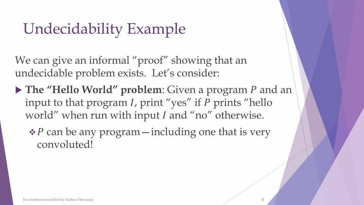
Undecidability Example
We can give an informal “proof” showing that an undecidable problem exists. Let’s consider:
The “Hello World” problem: Given a program 𝑃 and an input to that program 𝐼, print “yes” if 𝑃 prints “hello world” when run with input 𝐼 and “no” otherwise.
❖𝑃 can be any program—including one that is very convoluted!
Jim Anderson (modified by Nathan Otterness) 3
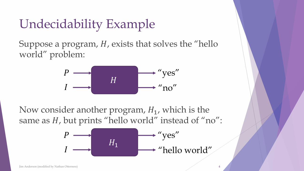
Undecidability Example
Suppose a program, 𝐻, exists that solves the “hello world” problem:
Now consider another program, 𝐻1, which is the same as 𝐻, but prints “hello world” instead of “no”:
Jim Anderson (modified by Nathan Otterness) 4
𝐻𝑃
𝐼
“yes”
“no”
𝐻1𝑃
𝐼
“yes”
“hello world”

Undecidability Example
Next, construct a program 𝐻2 that is identical to 𝐻1but only takes a single input, 𝑃, that it uses as both 𝑃and 𝐼 in 𝐻1:
Jim Anderson (modified by Nathan Otterness) 5
𝐻1𝑃
𝐼
“yes”
“hello world”
𝐻2𝑃“yes”
“hello world”
𝑃“yes”
“hello world”𝐻1
Another way to represent 𝐻2:
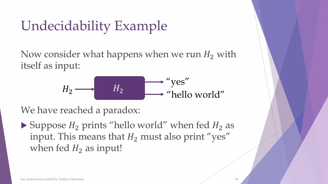
Undecidability Example
Now consider what happens when we run 𝐻2 with itself as input:
We have reached a paradox:
Suppose 𝐻2 prints “hello world” when fed 𝐻2 as input. This means that 𝐻2 must also print “yes” when fed 𝐻2 as input!
Jim Anderson (modified by Nathan Otterness) 6
𝐻2𝐻2“yes”
“hello world”
Turing Machines
To be able to rigorously do proofs like the “hello world” example, we need a formal model for defining computable functions.
The Turing Machine has become the accepted model for formalizing functions.
Jim Anderson (modified by Nathan Otterness) 7
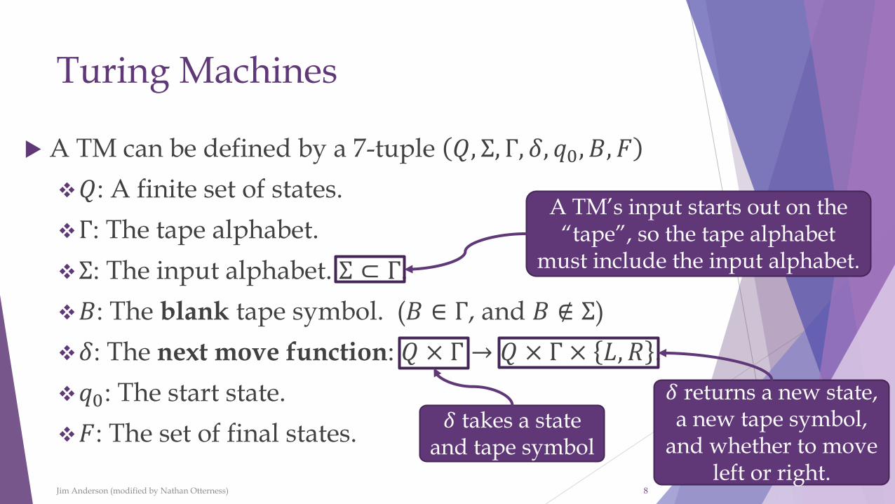
Turing Machines
A TM can be defined by a 7-tuple 𝑄, Σ, Γ, 𝛿, 𝑞0, 𝐵, 𝐹
❖𝑄: A finite set of states.
❖Γ: The tape alphabet.
❖Σ: The input alphabet. Σ ⊂ Γ.
❖𝐵: The blank tape symbol. (𝐵 ∈ Γ, and 𝐵 ∉ Σ)
❖𝛿: The next move function: 𝑄 × Γ → 𝑄 × Γ × 𝐿, 𝑅 .
❖𝑞0: The start state.
❖𝐹: The set of final states.
Jim Anderson (modified by Nathan Otterness) 8
A TM’s input starts out on the “tape”, so the tape alphabet
must include the input alphabet.
𝛿 takes a state and tape symbol
𝛿 returns a new state, a new tape symbol,
and whether to move left or right.

Turing Machines
Conceptually, a Turing Machine looks like this:
Jim Anderson (modified by Nathan Otterness) 9
𝑋1 𝑋𝑖… … 𝑋𝑛𝐵𝐵… 𝐵𝐵 …
Non-blank tape symbols (input symbols, etc.)
All of the rest of the tape initially is filled with “blank” symbols.
Finite Control
Tape head
Initially, the input starts out on the tape, and the tape head starts at the leftmost input symbol.
The “finite control” just refers to the part of the TM that keeps track of the state.
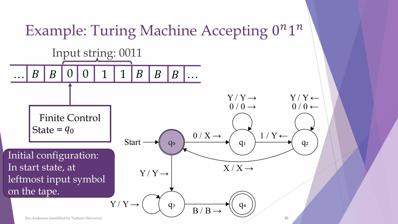
Example: Turing Machine Accepting 0𝑛1𝑛
Jim Anderson (modified by Nathan Otterness) 10
0𝐵𝐵… 𝐵𝐵 …
Finite ControlState =
0 1 1 𝐵
Input string: 0011
Initial configuration:In start state, at leftmost input symbol on the tape.
𝑞0
Example: Turing Machine Accepting 0𝑛1𝑛
Jim Anderson (modified by Nathan Otterness) 11
0𝐵𝐵… 𝐵𝐵 …
Finite ControlState =
0 1 1 𝐵
𝑞0
𝑋
𝑞1𝑞2
𝑌
𝑞0
𝑋
𝑞1
𝑌
𝑞2𝑞0 𝑞3 𝑞4
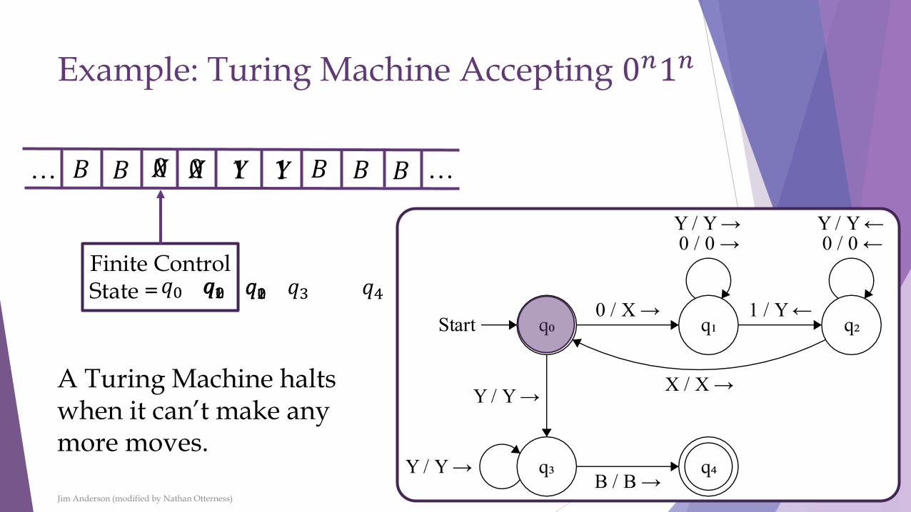
A Turing Machine halts when it can’t make any more moves.
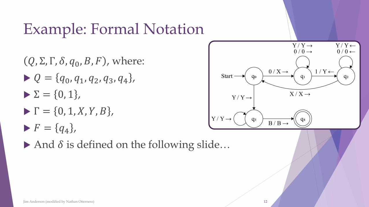
Example: Formal Notation
𝑄, Σ, Γ, 𝛿, 𝑞0, 𝐵, 𝐹 , where:
𝑄 = 𝑞0, 𝑞1, 𝑞2, 𝑞3, 𝑞4 ,
Σ = 0, 1 ,
Γ = 0, 1, 𝑋, 𝑌, 𝐵 ,
𝐹 = 𝑞4 ,
And 𝛿 is defined on the following slide…
Jim Anderson (modified by Nathan Otterness) 12
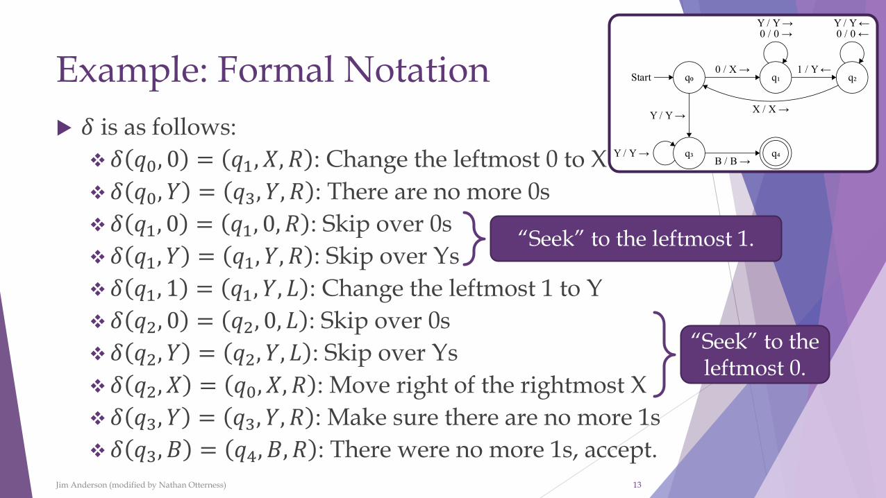
Example: Formal Notation
𝛿 is as follows:
❖𝛿 𝑞0, 0 = 𝑞1, 𝑋, 𝑅 : Change the leftmost 0 to X
❖𝛿 𝑞0, 𝑌 = 𝑞3, 𝑌, 𝑅 : There are no more 0s
❖𝛿 𝑞1, 0 = 𝑞1, 0, 𝑅 : Skip over 0s
❖𝛿 𝑞1, 𝑌 = 𝑞1, 𝑌, 𝑅 : Skip over Ys
❖𝛿 𝑞1, 1 = 𝑞1, 𝑌, 𝐿 : Change the leftmost 1 to Y
❖𝛿 𝑞2, 0 = 𝑞2, 0, 𝐿 : Skip over 0s
❖𝛿 𝑞2, 𝑌 = 𝑞2, 𝑌, 𝐿 : Skip over Ys
❖𝛿 𝑞2, 𝑋 = 𝑞0, 𝑋, 𝑅 : Move right of the rightmost X
❖𝛿 𝑞3, 𝑌 = 𝑞3, 𝑌, 𝑅 : Make sure there are no more 1s
❖𝛿 𝑞3, 𝐵 = 𝑞4, 𝐵, 𝑅 : There were no more 1s, accept.
Jim Anderson (modified by Nathan Otterness) 13
“Seek” to the leftmost 1.
“Seek” to the leftmost 0.

Instantaneous Descriptions for TMs
As with a PDA, we can also give an instantaneous description (ID) for a Turing Machine.
An ID for a TM has the following form: 𝛼1𝑞𝛼2.
❖𝑞 corresponds to both the state of the TM and the position of the tape head (𝑞 is written directly before the tape symbol the head is on).
❖𝛼1𝛼2 = the tape’s current contents, and only contains the non-blank portion, except in cases like 𝛼𝐵𝐵𝐵𝑞 or 𝑞𝐵𝐵𝐵𝛼.
The depicted portion of the tape is always finite.Jim Anderson (modified by Nathan Otterness) 14
This indicates both the location of the tape head and the current state (𝑞).
We can’t write an infinite number of cells without either infinite
input or an infinite number of moves.
Notation for TM Moves
Left moves. Suppose 𝛿 𝑞, 𝑋𝑖 = 𝑝, 𝑌, 𝐿 . Then,
❖𝑋1…𝑋𝑖−1𝑞𝑋𝑖 …𝑋𝑛├𝑀𝑋1…𝑋𝑖−2𝑝𝑋𝑖−1𝑌…𝑋𝑛.
❑The tape head moved from 𝑋𝑖 to 𝑋𝑖−1.
❑The state changed from 𝑞 to 𝑝.
❑𝑋𝑖 was replaced by 𝑌.
❖Special case where 𝑖 = 1:
❑𝑞𝑋1𝑋2…𝑋𝑛├𝑀𝑝𝐵𝑌𝑋2…𝑋𝑛
❖Special case where 𝑖 = 𝑛 and 𝑌 = 𝐵:
❑𝑋1…𝑋𝑛−1𝑞𝑋𝑛├𝑀𝑋1…𝑋𝑛−2𝑝𝑋𝑛−1
Jim Anderson (modified by Nathan Otterness) 15
We moved left past the start of the tape content, so we need to
show the extra blank symbol (𝐵).
We replaced the rightmost tape symbol (𝑋𝑛) with a 𝐵, so we no
longer include it in the ID.
Notation for TM Moves
Right moves. Suppose 𝛿 𝑞, 𝑋𝑖 = 𝑝, 𝑌, 𝑅 . Then,
❖𝑋1…𝑋𝑖−1𝑞𝑋𝑖 …𝑋𝑛├𝑀𝑋1…𝑋𝑖−1𝑌𝑝𝑋𝑖+1…𝑋𝑛.
❑The tape head moved from 𝑋𝑖 to 𝑋𝑖+1.
❑The state changed from 𝑞 to 𝑝.
❑𝑋𝑖 was replaced by 𝑌.
❖Special case where 𝑖 = 𝑛:
❑𝑋1…𝑋𝑛+1𝑞𝑋𝑛├𝑀𝑋1…𝑋𝑛−1𝑌𝑝𝐵.
❖Special case where 𝑖 = 1 and 𝑌 = 𝐵:
❑𝑞𝑋1…𝑋𝑛├𝑀𝑝𝑋2…𝑋𝑛.
Jim Anderson (modified by Nathan Otterness) 16
The 𝐵 is included here just to make it clear what the tape head is pointing at.
The Language Defined by a TM
The language accepted by a Turing Machine 𝑀 is defined as:
𝐿 𝑀 ≡ {𝑤 | 𝑤 ∈ Σ∗ and 𝑞0𝑤 ├𝑀
∗𝛼1𝑝𝛼2 for some 𝑝 ∈ 𝐹, and
𝛼1, 𝛼2 ∈ Γ∗}.
Assumption: If 𝑀 accepts 𝑤, 𝑀 halts.
Notation used for moves (similar to a PDA):
❖├𝑀
𝑖, ├𝑀
∗, ├, ├
𝑖, ├∗
.
❑The 𝑖 indicates “exactly 𝑖 moves”
❑The ∗ indicates “any number of moves”
❑The (optional) 𝑀 below the ├ indicates that TM 𝑀 made the moves.
Jim Anderson (modified by Nathan Otterness) 17
Recursively Enumerable Languages
A language that is accepted by a Turing Machine is called recursively enumerable (RE).
If a string 𝑤 is in 𝐿 𝑀 , then 𝑀 eventually halts and accepts 𝑤.
If 𝑤 ∉ 𝐿 𝑀 , then one of two things can happen:
❖𝑀 halts without accepting 𝑤, or
❖𝑀 never halts.
Jim Anderson (modified by Nathan Otterness) 18
Recursive Languages
A language that is accepted by a TM that halts on all inputs is called recursive.
This is the accepted formal definition of “algorithm”.
❖For a recursive language, we can always algorithmically determine membership—but we can’t necessarily do this for RE languages.
A problem that is solved by a TM that always halts is called decidable.
❖We will discuss decidable problems in much more detail later!
Jim Anderson (modified by Nathan Otterness) 19
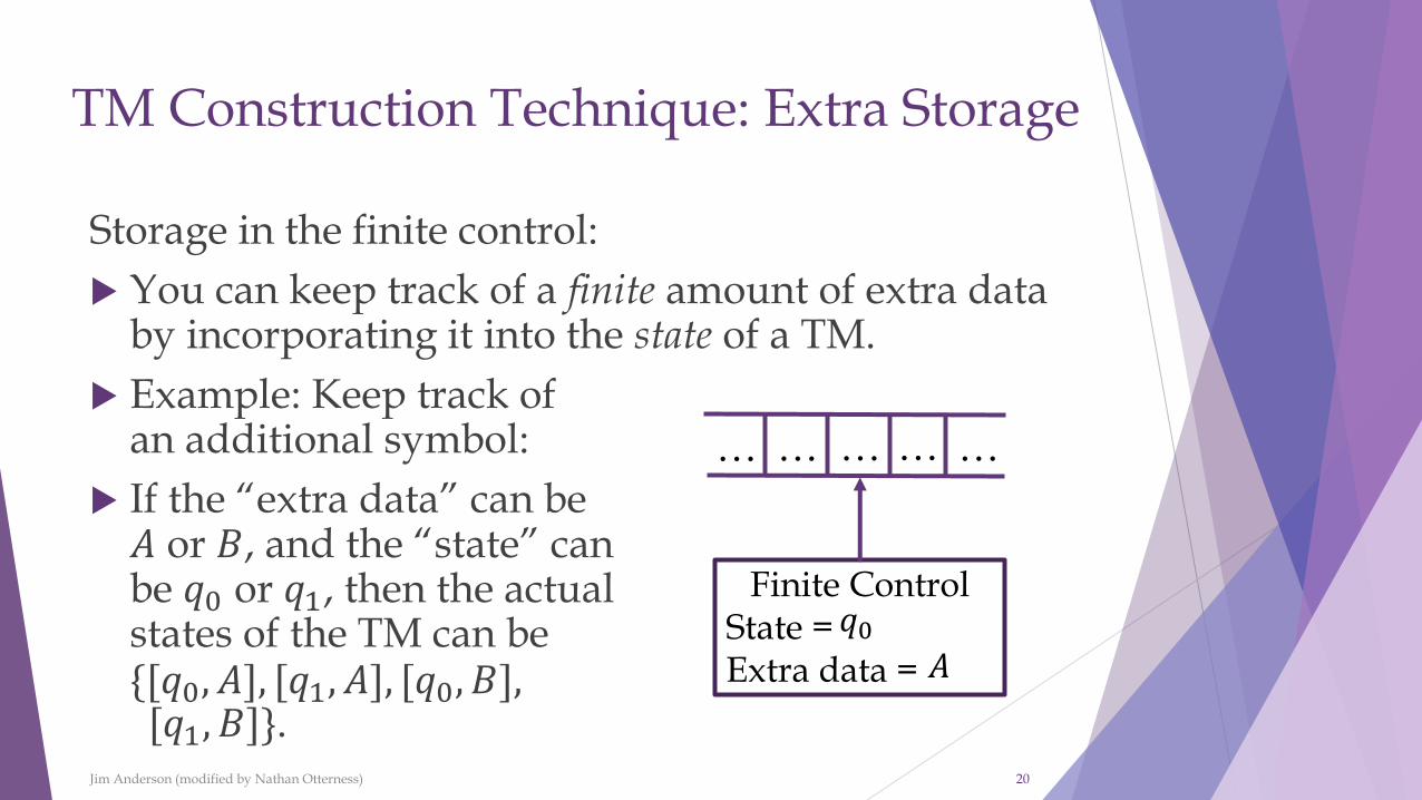
TM Construction Technique: Extra Storage
Storage in the finite control:
You can keep track of a finite amount of extra data by incorporating it into the state of a TM.
Example: Keep track ofan additional symbol:
If the “extra data” can be𝐴 or 𝐵, and the “state” canbe 𝑞0 or 𝑞1, then the actualstates of the TM can be{[𝑞0, 𝐴], [𝑞1, 𝐴], [𝑞0, 𝐵],[𝑞1, 𝐵]}.
Jim Anderson (modified by Nathan Otterness) 20
… …
Finite ControlState =Extra data =
𝑞0𝐴
… … …
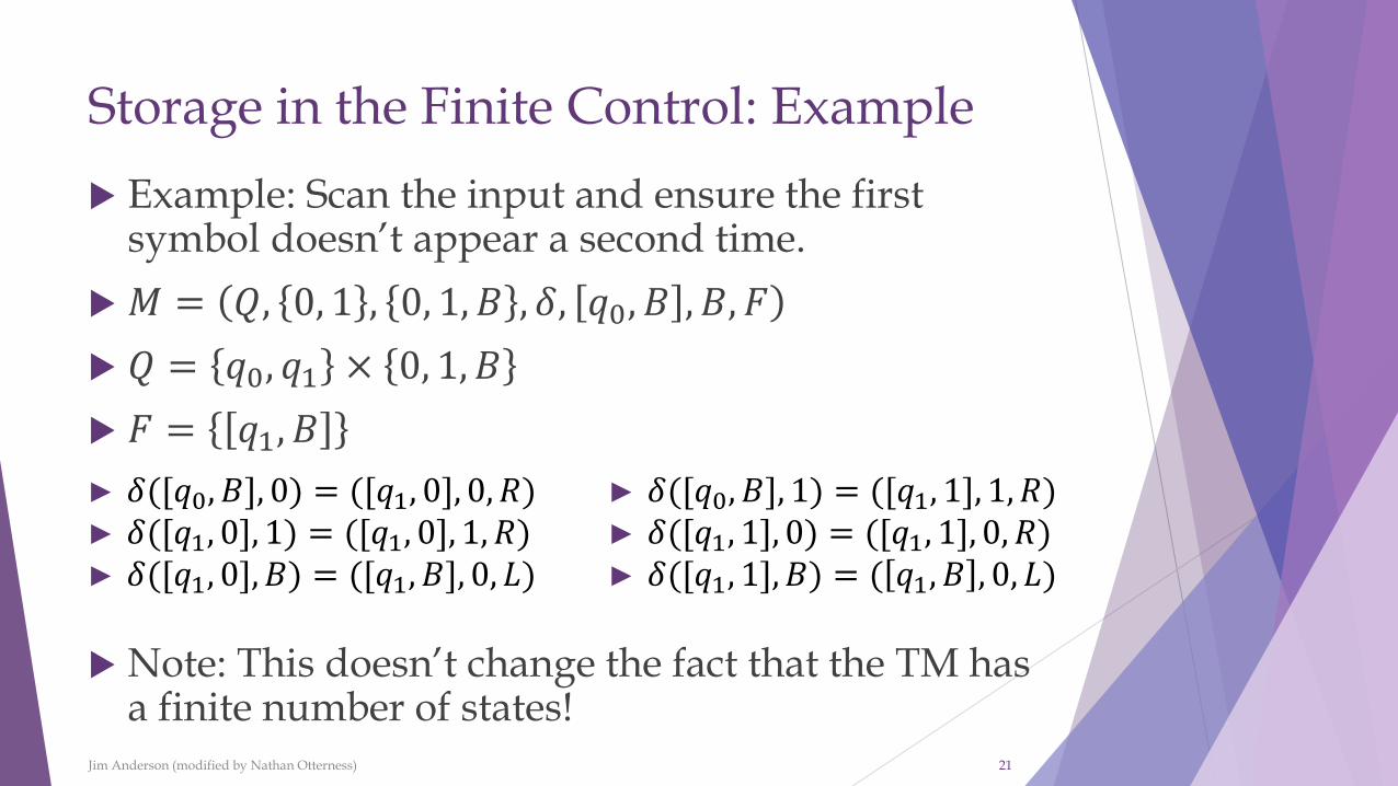
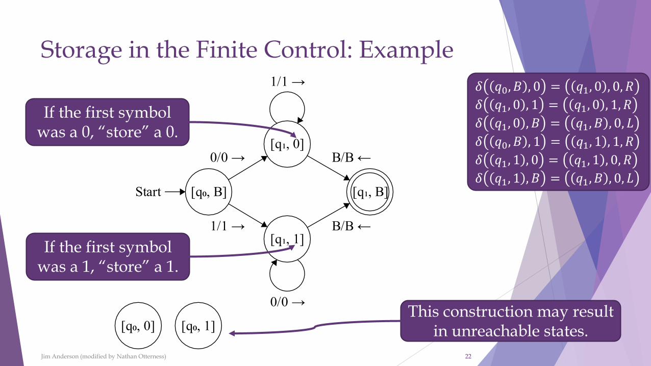
Storage in the Finite Control: Example
Example: Scan the input and ensure the first symbol doesn’t appear a second time.
𝑀 = 𝑄, 0, 1 , 0, 1, 𝐵 , 𝛿, 𝑞0, 𝐵 , 𝐵, 𝐹
𝑄 = 𝑞0, 𝑞1 × 0, 1, 𝐵
𝐹 = 𝑞1, 𝐵
Note: This doesn’t change the fact that the TM has a finite number of states!
Jim Anderson (modified by Nathan Otterness) 21
► 𝛿([𝑞0, 𝐵], 0) = ([𝑞1, 0], 0, 𝑅)► 𝛿([𝑞1, 0], 1) = ([𝑞1, 0], 1, 𝑅)► 𝛿([𝑞1, 0], 𝐵) = ([𝑞1, 𝐵], 0, 𝐿)
► 𝛿([𝑞0, 𝐵], 1) = ([𝑞1, 1], 1, 𝑅)► 𝛿([𝑞1, 1], 0) = ([𝑞1, 1], 0, 𝑅)► 𝛿([𝑞1, 1], 𝐵) = ( 𝑞1, 𝐵 , 0, 𝐿)
Storage in the Finite Control: Example
Jim Anderson (modified by Nathan Otterness) 22
𝛿 𝑞0, 𝐵 , 0 = 𝑞1, 0 , 0, 𝑅
𝛿 𝑞1, 0 , 1 = 𝑞1, 0 , 1, 𝑅
𝛿 𝑞1, 0 , 𝐵 = 𝑞1, 𝐵 , 0, 𝐿
𝛿 𝑞0, 𝐵 , 1 = 𝑞1, 1 , 1, 𝑅
𝛿 𝑞1, 1 , 0 = 𝑞1, 1 , 0, 𝑅
𝛿 𝑞1, 1 , 𝐵 = 𝑞1, 𝐵 , 0, 𝐿
If the first symbol was a 0, “store” a 0.
If the first symbol was a 1, “store” a 1.
This construction may result in unreachable states.
Jim Anderson (modified by Nathan Otterness) 23
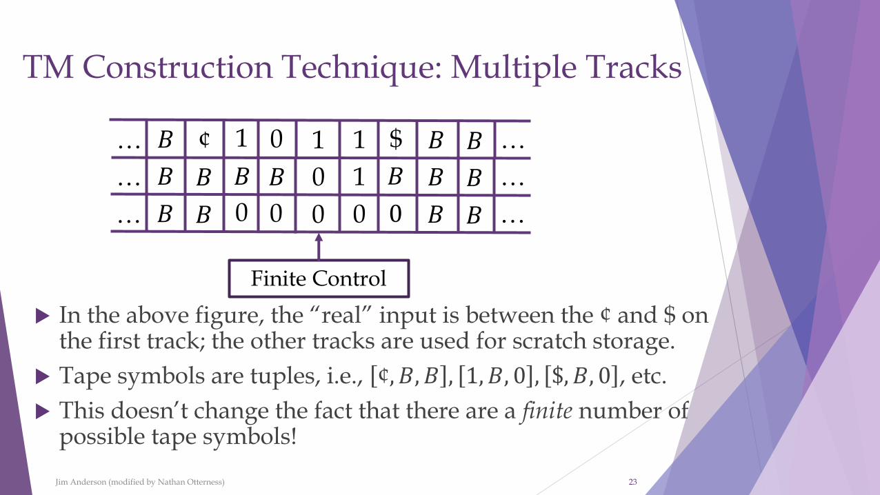
TM Construction Technique: Multiple Tracks
0¢𝐵… 𝐵𝐵 …
Finite Control
1 1 1 $
𝐵𝐵… 𝐵𝐵 …0 1 𝐵
0𝐵𝐵… 𝐵𝐵 …0 0 0 0
𝐵 𝐵
In the above figure, the “real” input is between the ¢ and $ on the first track; the other tracks are used for scratch storage.
Tape symbols are tuples, i.e., ¢, 𝐵, 𝐵 , 1, 𝐵, 0 , $, 𝐵, 0 , etc.
This doesn’t change the fact that there are a finite number of possible tape symbols!
Multiple Tracks: Example
We will use multiple tracks and storage in the finite control to write a TM that accepts the language 𝐿 = 𝑤𝑐𝑤 | 𝑤 ∈ 𝐚 + 𝐛 ∗ .
This TM will work by “checking off” corresponding symbols in each copy of 𝑤.
Jim Anderson (modified by Nathan Otterness) 24
Any string 𝑤, followed by a “c”, followed by a second copy of 𝑤.
Multiple Tracks: Example
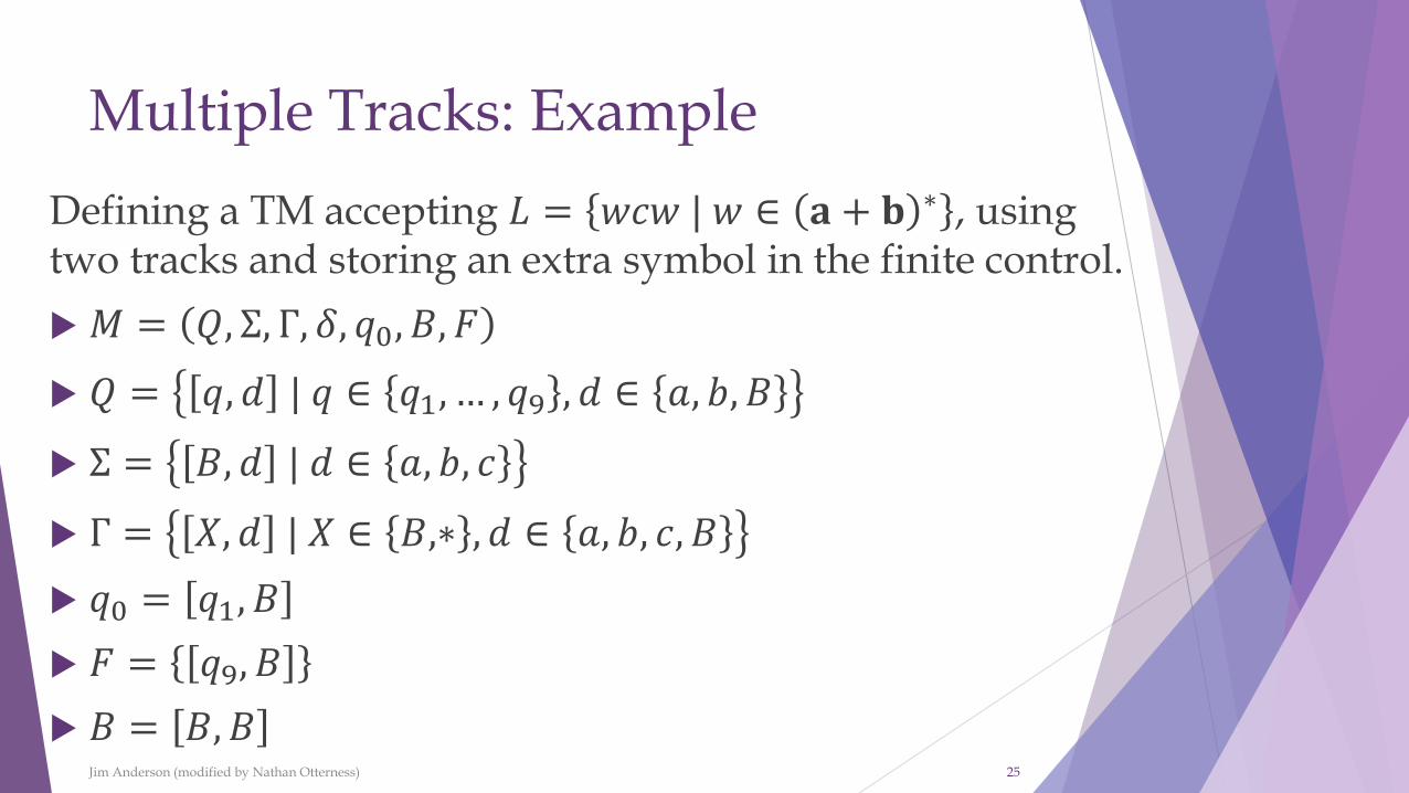
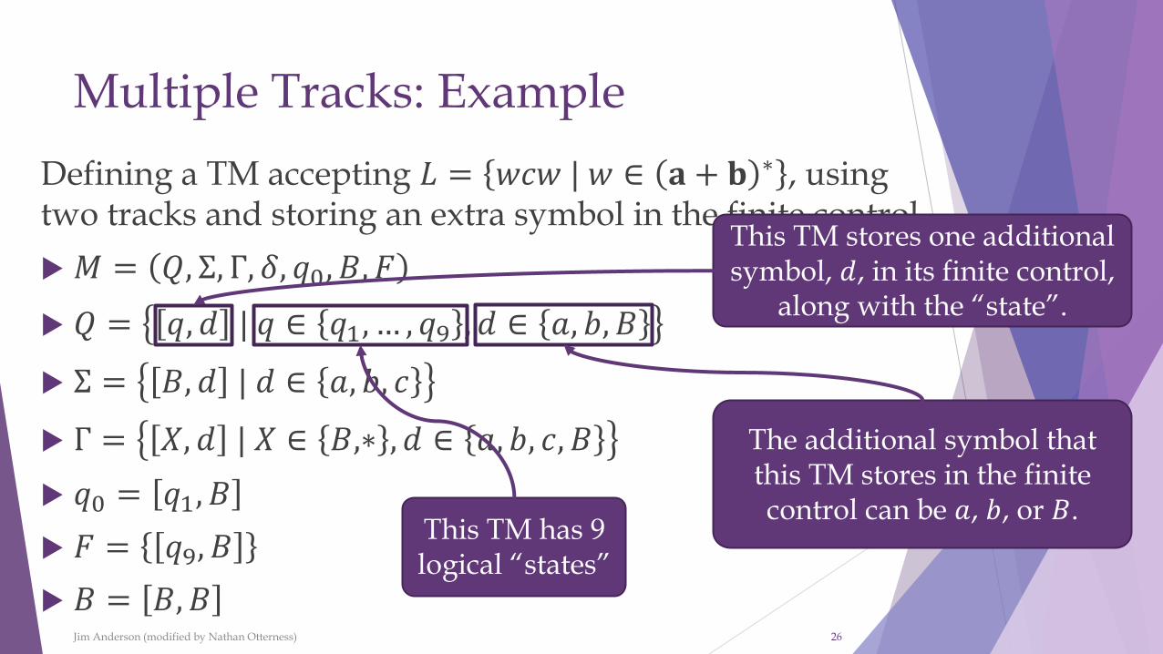
Defining a TM accepting 𝐿 = 𝑤𝑐𝑤 | 𝑤 ∈ 𝐚 + 𝐛 ∗ , using two tracks and storing an extra symbol in the finite control.
𝑀 = 𝑄, Σ, Γ, 𝛿, 𝑞0, 𝐵, 𝐹
𝑄 = 𝑞, 𝑑 | 𝑞 ∈ 𝑞1, … , 𝑞9 , 𝑑 ∈ 𝑎, 𝑏, 𝐵
Σ = 𝐵, 𝑑 | 𝑑 ∈ 𝑎, 𝑏, 𝑐
Γ = 𝑋, 𝑑 | 𝑋 ∈ 𝐵,∗ , 𝑑 ∈ 𝑎, 𝑏, 𝑐, 𝐵
𝑞0 = 𝑞1, 𝐵
𝐹 = 𝑞9, 𝐵
𝐵 = 𝐵, 𝐵Jim Anderson (modified by Nathan Otterness) 25
Multiple Tracks: Example
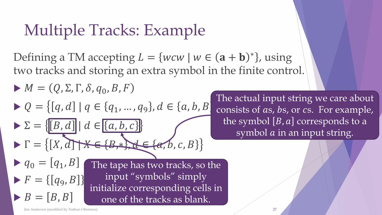
Defining a TM accepting 𝐿 = 𝑤𝑐𝑤 | 𝑤 ∈ 𝐚 + 𝐛 ∗ , using two tracks and storing an extra symbol in the finite control.
𝑀 = 𝑄, Σ, Γ, 𝛿, 𝑞0, 𝐵, 𝐹
𝑄 = 𝑞, 𝑑 | 𝑞 ∈ 𝑞1, … , 𝑞9 , 𝑑 ∈ 𝑎, 𝑏, 𝐵
Σ = 𝐵, 𝑑 | 𝑑 ∈ 𝑎, 𝑏, 𝑐
Γ = 𝑋, 𝑑 | 𝑋 ∈ 𝐵,∗ , 𝑑 ∈ 𝑎, 𝑏, 𝑐, 𝐵
𝑞0 = 𝑞1, 𝐵
𝐹 = 𝑞9, 𝐵
𝐵 = 𝐵, 𝐵Jim Anderson (modified by Nathan Otterness) 26
This TM stores one additional symbol, 𝑑, in its finite control,
along with the “state”.
This TM has 9 logical “states”
The additional symbol that this TM stores in the finite control can be 𝑎, 𝑏, or 𝐵.
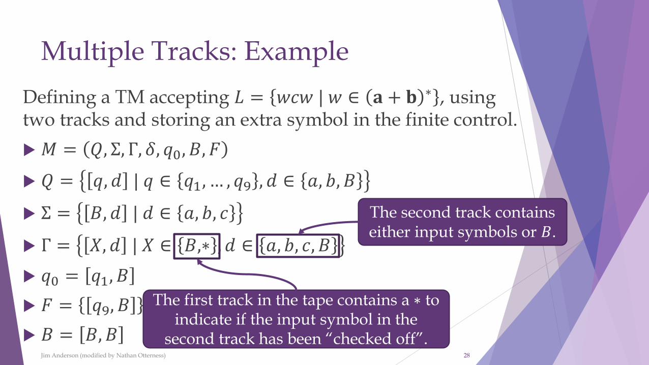
Multiple Tracks: Example
Defining a TM accepting 𝐿 = 𝑤𝑐𝑤 | 𝑤 ∈ 𝐚 + 𝐛 ∗ , using two tracks and storing an extra symbol in the finite control.
𝑀 = 𝑄, Σ, Γ, 𝛿, 𝑞0, 𝐵, 𝐹
𝑄 = 𝑞, 𝑑 | 𝑞 ∈ 𝑞1, … , 𝑞9 , 𝑑 ∈ 𝑎, 𝑏, 𝐵
Σ = 𝐵, 𝑑 | 𝑑 ∈ 𝑎, 𝑏, 𝑐
Γ = 𝑋, 𝑑 | 𝑋 ∈ 𝐵,∗ , 𝑑 ∈ 𝑎, 𝑏, 𝑐, 𝐵
𝑞0 = 𝑞1, 𝐵
𝐹 = 𝑞9, 𝐵
𝐵 = 𝐵, 𝐵Jim Anderson (modified by Nathan Otterness) 27
The tape has two tracks, so the input “symbols” simply
initialize corresponding cells in one of the tracks as blank.
The actual input string we care about consists of 𝑎s, 𝑏s, or 𝑐s. For example,
the symbol 𝐵, 𝑎 corresponds to a symbol 𝑎 in an input string.
Multiple Tracks: Example
Defining a TM accepting 𝐿 = 𝑤𝑐𝑤 | 𝑤 ∈ 𝐚 + 𝐛 ∗ , using two tracks and storing an extra symbol in the finite control.
𝑀 = 𝑄, Σ, Γ, 𝛿, 𝑞0, 𝐵, 𝐹
𝑄 = 𝑞, 𝑑 | 𝑞 ∈ 𝑞1, … , 𝑞9 , 𝑑 ∈ 𝑎, 𝑏, 𝐵
Σ = 𝐵, 𝑑 | 𝑑 ∈ 𝑎, 𝑏, 𝑐
Γ = 𝑋, 𝑑 | 𝑋 ∈ 𝐵,∗ , 𝑑 ∈ 𝑎, 𝑏, 𝑐, 𝐵
𝑞0 = 𝑞1, 𝐵
𝐹 = 𝑞9, 𝐵
𝐵 = 𝐵, 𝐵Jim Anderson (modified by Nathan Otterness) 28
The first track in the tape contains a ∗ to indicate if the input symbol in the
second track has been “checked off”.
The second track contains either input symbols or 𝐵.
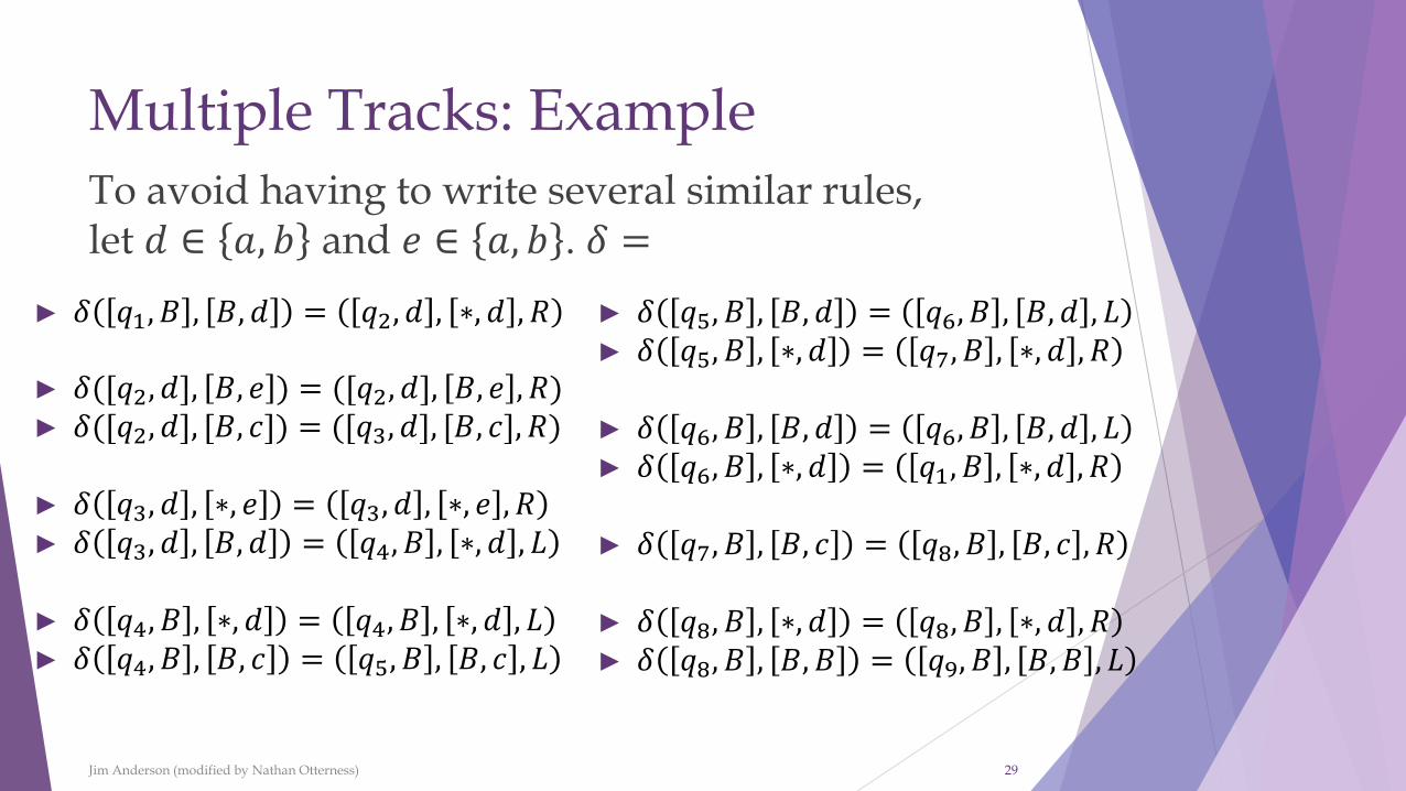
Multiple Tracks: ExampleTo avoid having to write several similar rules,let 𝑑 ∈ 𝑎, 𝑏 and 𝑒 ∈ 𝑎, 𝑏 . 𝛿 =
Jim Anderson (modified by Nathan Otterness) 29
► 𝛿 𝑞1, 𝐵 , 𝐵, 𝑑 = 𝑞2, 𝑑 , ∗, 𝑑 , 𝑅
► 𝛿([𝑞2, 𝑑], 𝐵, 𝑒 ) = ([𝑞2, 𝑑], 𝐵, 𝑒 , 𝑅)► 𝛿([𝑞2, 𝑑], [𝐵, 𝑐]) = ([𝑞3, 𝑑], [𝐵, 𝑐], 𝑅)
► 𝛿 𝑞3, 𝑑 , ∗, 𝑒 = 𝑞3, 𝑑 , ∗, 𝑒 , 𝑅► 𝛿 𝑞3, 𝑑 , 𝐵, 𝑑 = 𝑞4, 𝐵 , ∗, 𝑑 , 𝐿
► 𝛿 𝑞4, 𝐵 , ∗, 𝑑 = 𝑞4, 𝐵 , ∗, 𝑑 , 𝐿► 𝛿 𝑞4, 𝐵 , 𝐵, 𝑐 = 𝑞5, 𝐵 , 𝐵, 𝑐 , 𝐿
► 𝛿 𝑞5, 𝐵 , 𝐵, 𝑑 = 𝑞6, 𝐵 , 𝐵, 𝑑 , 𝐿► 𝛿 𝑞5, 𝐵 , ∗, 𝑑 = 𝑞7, 𝐵 , ∗, 𝑑 , 𝑅
► 𝛿 𝑞6, 𝐵 , 𝐵, 𝑑 = 𝑞6, 𝐵 , 𝐵, 𝑑 , 𝐿► 𝛿 𝑞6, 𝐵 , ∗, 𝑑 = 𝑞1, 𝐵 , ∗, 𝑑 , 𝑅
► 𝛿 𝑞7, 𝐵 , 𝐵, 𝑐 = 𝑞8, 𝐵 , 𝐵, 𝑐 , 𝑅
► 𝛿 𝑞8, 𝐵 , ∗, 𝑑 = 𝑞8, 𝐵 , ∗, 𝑑 , 𝑅► 𝛿 𝑞8, 𝐵 , 𝐵, 𝐵 = 𝑞9, 𝐵 , 𝐵, 𝐵 , 𝐿
Multiple Tracks: Example
(Let 𝑑 ∈ 𝑎, 𝑏 and 𝑒 ∈ 𝑎, 𝑏 .)
Jim Anderson (modified by Nathan Otterness) 30
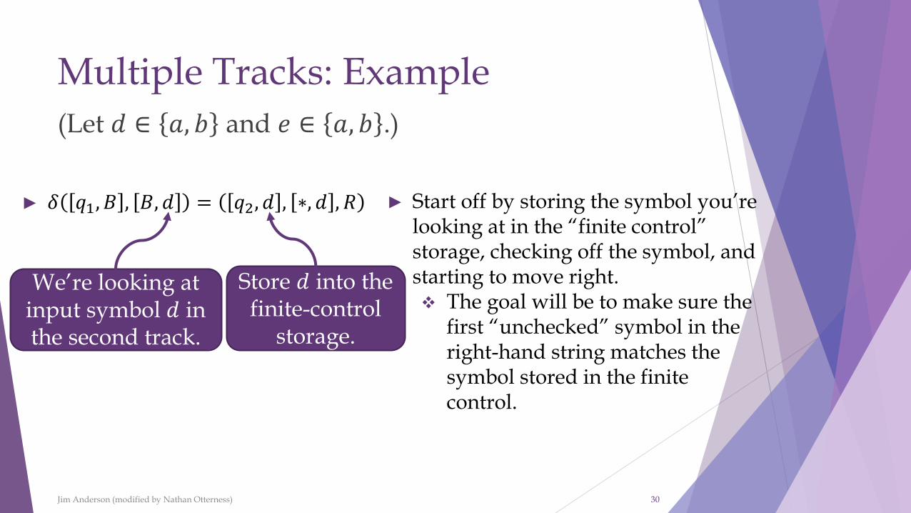
► 𝛿 𝑞1, 𝐵 , 𝐵, 𝑑 = 𝑞2, 𝑑 , ∗, 𝑑 , 𝑅 ► Start off by storing the symbol you’re looking at in the “finite control” storage, checking off the symbol, and starting to move right.❖ The goal will be to make sure the
first “unchecked” symbol in the right-hand string matches the symbol stored in the finite control.
We’re looking at input symbol 𝑑 in the second track.
Store 𝑑 into the finite-control
storage.

Multiple Tracks: Example
(Let 𝑑 ∈ 𝑎, 𝑏 and 𝑒 ∈ 𝑎, 𝑏 .)
Jim Anderson (modified by Nathan Otterness) 31
► 𝛿 𝑞1, 𝐵 , 𝐵, 𝑑 = 𝑞2, 𝑑 , ∗, 𝑑 , 𝑅 ► Start off by storing the symbol you’re looking at in the “finite control” storage, checking off the symbol, and starting to move right.❖ The goal will be to make sure the
first “unchecked” symbol in the right-hand string matches the symbol stored in the finite control.
Previously, this symbol was not checked off…
So we’ll check it off.
Multiple Tracks: Example
Jim Anderson (modified by Nathan Otterness) 32
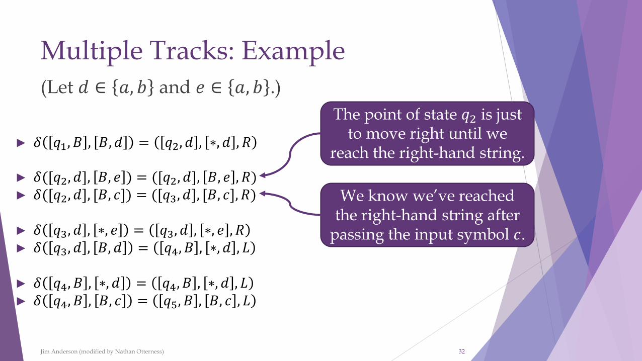
► 𝛿 𝑞1, 𝐵 , 𝐵, 𝑑 = 𝑞2, 𝑑 , ∗, 𝑑 , 𝑅
► 𝛿([𝑞2, 𝑑], 𝐵, 𝑒 ) = ([𝑞2, 𝑑], 𝐵, 𝑒 , 𝑅)► 𝛿([𝑞2, 𝑑], [𝐵, 𝑐]) = ([𝑞3, 𝑑], [𝐵, 𝑐], 𝑅)
► 𝛿 𝑞3, 𝑑 , ∗, 𝑒 = 𝑞3, 𝑑 , ∗, 𝑒 , 𝑅► 𝛿 𝑞3, 𝑑 , 𝐵, 𝑑 = 𝑞4, 𝐵 , ∗, 𝑑 , 𝐿
► 𝛿 𝑞4, 𝐵 , ∗, 𝑑 = 𝑞4, 𝐵 , ∗, 𝑑 , 𝐿► 𝛿 𝑞4, 𝐵 , 𝐵, 𝑐 = 𝑞5, 𝐵 , 𝐵, 𝑐 , 𝐿
(Let 𝑑 ∈ 𝑎, 𝑏 and 𝑒 ∈ 𝑎, 𝑏 .)
The point of state 𝑞2 is just to move right until we
reach the right-hand string.
We know we’ve reached the right-hand string after
passing the input symbol 𝑐.
Multiple Tracks: Example
Jim Anderson (modified by Nathan Otterness) 33
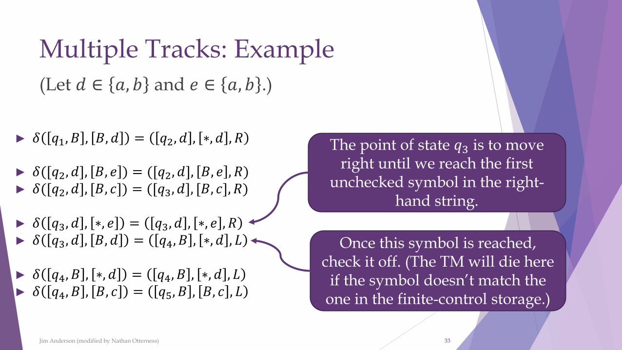
► 𝛿 𝑞1, 𝐵 , 𝐵, 𝑑 = 𝑞2, 𝑑 , ∗, 𝑑 , 𝑅
► 𝛿([𝑞2, 𝑑], 𝐵, 𝑒 ) = ([𝑞2, 𝑑], 𝐵, 𝑒 , 𝑅)► 𝛿([𝑞2, 𝑑], [𝐵, 𝑐]) = ([𝑞3, 𝑑], [𝐵, 𝑐], 𝑅)
► 𝛿 𝑞3, 𝑑 , ∗, 𝑒 = 𝑞3, 𝑑 , ∗, 𝑒 , 𝑅► 𝛿 𝑞3, 𝑑 , 𝐵, 𝑑 = 𝑞4, 𝐵 , ∗, 𝑑 , 𝐿
► 𝛿 𝑞4, 𝐵 , ∗, 𝑑 = 𝑞4, 𝐵 , ∗, 𝑑 , 𝐿► 𝛿 𝑞4, 𝐵 , 𝐵, 𝑐 = 𝑞5, 𝐵 , 𝐵, 𝑐 , 𝐿
(Let 𝑑 ∈ 𝑎, 𝑏 and 𝑒 ∈ 𝑎, 𝑏 .)
The point of state 𝑞3 is to move right until we reach the first
unchecked symbol in the right-hand string.
Once this symbol is reached, check it off. (The TM will die here
if the symbol doesn’t match the one in the finite-control storage.)
Multiple Tracks: Example
Jim Anderson (modified by Nathan Otterness) 34
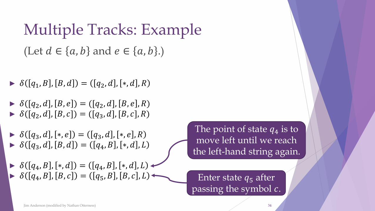
► 𝛿 𝑞1, 𝐵 , 𝐵, 𝑑 = 𝑞2, 𝑑 , ∗, 𝑑 , 𝑅
► 𝛿([𝑞2, 𝑑], 𝐵, 𝑒 ) = ([𝑞2, 𝑑], 𝐵, 𝑒 , 𝑅)► 𝛿([𝑞2, 𝑑], [𝐵, 𝑐]) = ([𝑞3, 𝑑], [𝐵, 𝑐], 𝑅)
► 𝛿 𝑞3, 𝑑 , ∗, 𝑒 = 𝑞3, 𝑑 , ∗, 𝑒 , 𝑅► 𝛿 𝑞3, 𝑑 , 𝐵, 𝑑 = 𝑞4, 𝐵 , ∗, 𝑑 , 𝐿
► 𝛿 𝑞4, 𝐵 , ∗, 𝑑 = 𝑞4, 𝐵 , ∗, 𝑑 , 𝐿► 𝛿 𝑞4, 𝐵 , 𝐵, 𝑐 = 𝑞5, 𝐵 , 𝐵, 𝑐 , 𝐿
(Let 𝑑 ∈ 𝑎, 𝑏 and 𝑒 ∈ 𝑎, 𝑏 .)
The point of state 𝑞4 is to move left until we reach
the left-hand string again.
Enter state 𝑞5 after passing the symbol 𝑐.
Multiple Tracks: Example
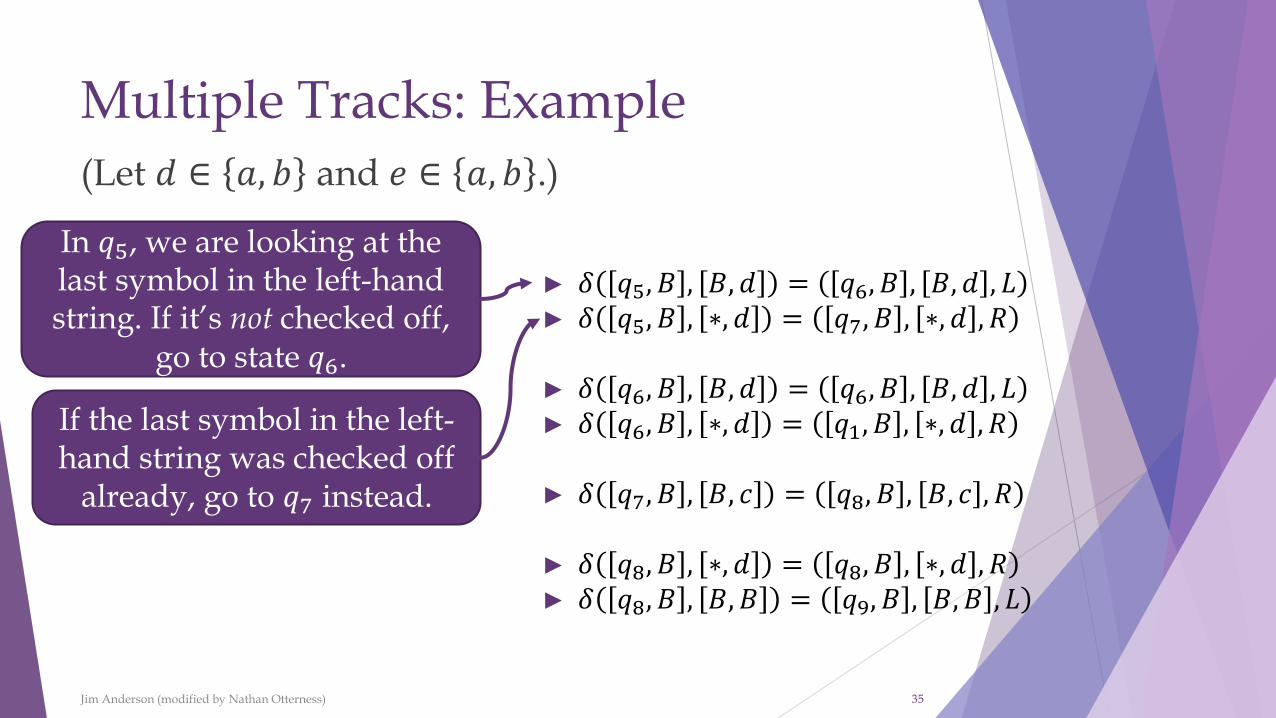
Jim Anderson (modified by Nathan Otterness) 35
(Let 𝑑 ∈ 𝑎, 𝑏 and 𝑒 ∈ 𝑎, 𝑏 .)
In 𝑞5, we are looking at the last symbol in the left-hand string. If it’s not checked off,
go to state 𝑞6.
If the last symbol in the left-hand string was checked off
already, go to 𝑞7 instead.
► 𝛿 𝑞5, 𝐵 , 𝐵, 𝑑 = 𝑞6, 𝐵 , 𝐵, 𝑑 , 𝐿► 𝛿 𝑞5, 𝐵 , ∗, 𝑑 = 𝑞7, 𝐵 , ∗, 𝑑 , 𝑅
► 𝛿 𝑞6, 𝐵 , 𝐵, 𝑑 = 𝑞6, 𝐵 , 𝐵, 𝑑 , 𝐿► 𝛿 𝑞6, 𝐵 , ∗, 𝑑 = 𝑞1, 𝐵 , ∗, 𝑑 , 𝑅
► 𝛿 𝑞7, 𝐵 , 𝐵, 𝑐 = 𝑞8, 𝐵 , 𝐵, 𝑐 , 𝑅
► 𝛿 𝑞8, 𝐵 , ∗, 𝑑 = 𝑞8, 𝐵 , ∗, 𝑑 , 𝑅► 𝛿 𝑞8, 𝐵 , 𝐵, 𝐵 = 𝑞9, 𝐵 , 𝐵, 𝐵 , 𝐿
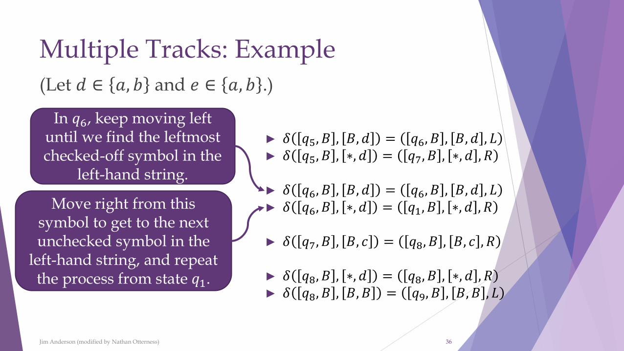
Multiple Tracks: Example
Jim Anderson (modified by Nathan Otterness) 36
(Let 𝑑 ∈ 𝑎, 𝑏 and 𝑒 ∈ 𝑎, 𝑏 .)
In 𝑞6, keep moving left until we find the leftmost checked-off symbol in the
left-hand string.
Move right from this symbol to get to the next unchecked symbol in the
left-hand string, and repeat the process from state 𝑞1.
► 𝛿 𝑞5, 𝐵 , 𝐵, 𝑑 = 𝑞6, 𝐵 , 𝐵, 𝑑 , 𝐿► 𝛿 𝑞5, 𝐵 , ∗, 𝑑 = 𝑞7, 𝐵 , ∗, 𝑑 , 𝑅
► 𝛿 𝑞6, 𝐵 , 𝐵, 𝑑 = 𝑞6, 𝐵 , 𝐵, 𝑑 , 𝐿► 𝛿 𝑞6, 𝐵 , ∗, 𝑑 = 𝑞1, 𝐵 , ∗, 𝑑 , 𝑅
► 𝛿 𝑞7, 𝐵 , 𝐵, 𝑐 = 𝑞8, 𝐵 , 𝐵, 𝑐 , 𝑅
► 𝛿 𝑞8, 𝐵 , ∗, 𝑑 = 𝑞8, 𝐵 , ∗, 𝑑 , 𝑅► 𝛿 𝑞8, 𝐵 , 𝐵, 𝐵 = 𝑞9, 𝐵 , 𝐵, 𝐵 , 𝐿
Multiple Tracks: Example
Jim Anderson (modified by Nathan Otterness) 37
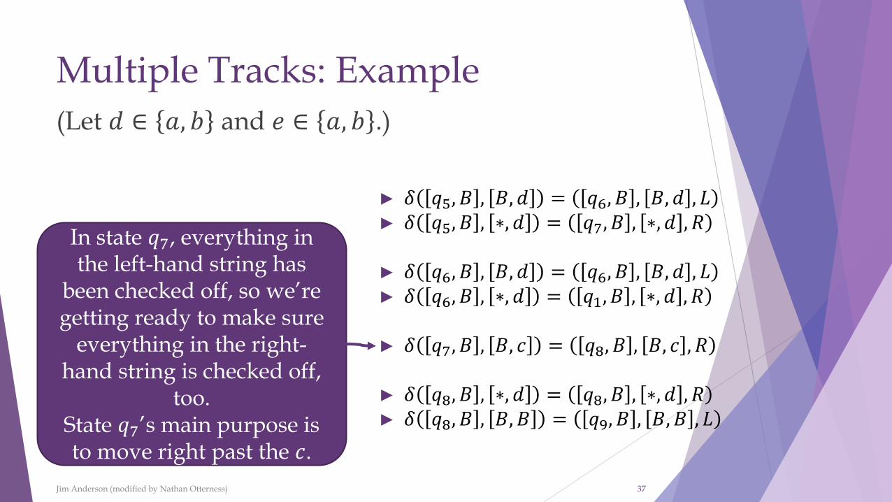
(Let 𝑑 ∈ 𝑎, 𝑏 and 𝑒 ∈ 𝑎, 𝑏 .)
In state 𝑞7, everything in the left-hand string has
been checked off, so we’re getting ready to make sure
everything in the right-hand string is checked off,
too.State 𝑞7’s main purpose is to move right past the 𝑐.
► 𝛿 𝑞5, 𝐵 , 𝐵, 𝑑 = 𝑞6, 𝐵 , 𝐵, 𝑑 , 𝐿► 𝛿 𝑞5, 𝐵 , ∗, 𝑑 = 𝑞7, 𝐵 , ∗, 𝑑 , 𝑅
► 𝛿 𝑞6, 𝐵 , 𝐵, 𝑑 = 𝑞6, 𝐵 , 𝐵, 𝑑 , 𝐿► 𝛿 𝑞6, 𝐵 , ∗, 𝑑 = 𝑞1, 𝐵 , ∗, 𝑑 , 𝑅
► 𝛿 𝑞7, 𝐵 , 𝐵, 𝑐 = 𝑞8, 𝐵 , 𝐵, 𝑐 , 𝑅
► 𝛿 𝑞8, 𝐵 , ∗, 𝑑 = 𝑞8, 𝐵 , ∗, 𝑑 , 𝑅► 𝛿 𝑞8, 𝐵 , 𝐵, 𝐵 = 𝑞9, 𝐵 , 𝐵, 𝐵 , 𝐿
Multiple Tracks: Example
Jim Anderson (modified by Nathan Otterness) 38
(Let 𝑑 ∈ 𝑎, 𝑏 and 𝑒 ∈ 𝑎, 𝑏 .)
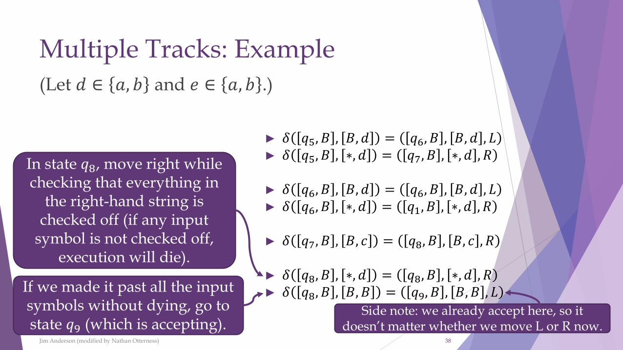
In state 𝑞8, move right while checking that everything in
the right-hand string is checked off (if any input
symbol is not checked off, execution will die).
► 𝛿 𝑞5, 𝐵 , 𝐵, 𝑑 = 𝑞6, 𝐵 , 𝐵, 𝑑 , 𝐿► 𝛿 𝑞5, 𝐵 , ∗, 𝑑 = 𝑞7, 𝐵 , ∗, 𝑑 , 𝑅
► 𝛿 𝑞6, 𝐵 , 𝐵, 𝑑 = 𝑞6, 𝐵 , 𝐵, 𝑑 , 𝐿► 𝛿 𝑞6, 𝐵 , ∗, 𝑑 = 𝑞1, 𝐵 , ∗, 𝑑 , 𝑅
► 𝛿 𝑞7, 𝐵 , 𝐵, 𝑐 = 𝑞8, 𝐵 , 𝐵, 𝑐 , 𝑅
► 𝛿 𝑞8, 𝐵 , ∗, 𝑑 = 𝑞8, 𝐵 , ∗, 𝑑 , 𝑅► 𝛿 𝑞8, 𝐵 , 𝐵, 𝐵 = 𝑞9, 𝐵 , 𝐵, 𝐵 , 𝐿If we made it past all the input
symbols without dying, go to state 𝑞9 (which is accepting).
Side note: we already accept here, so it doesn’t matter whether we move L or R now.
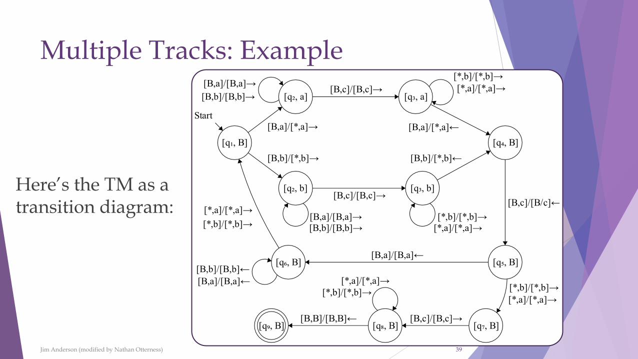
Multiple Tracks: Example
Here’s the TM as a transition diagram:
Jim Anderson (modified by Nathan Otterness) 39

TM Technique: Shifting Symbols Over
You may need to create extra space in the middle of a string of symbols in a TM.
This can be accomplished by holding a small buffer of symbols in the finite control.
Example: Shifting a string of nonblank symbols over by two spaces.
❖States will be of the form 𝑞, 𝐴1, 𝐴2 , where 𝑞 is 𝑞1 or 𝑞2 and 𝐴1 and 𝐴2 are in Γ.
Jim Anderson (modified by Nathan Otterness) 40

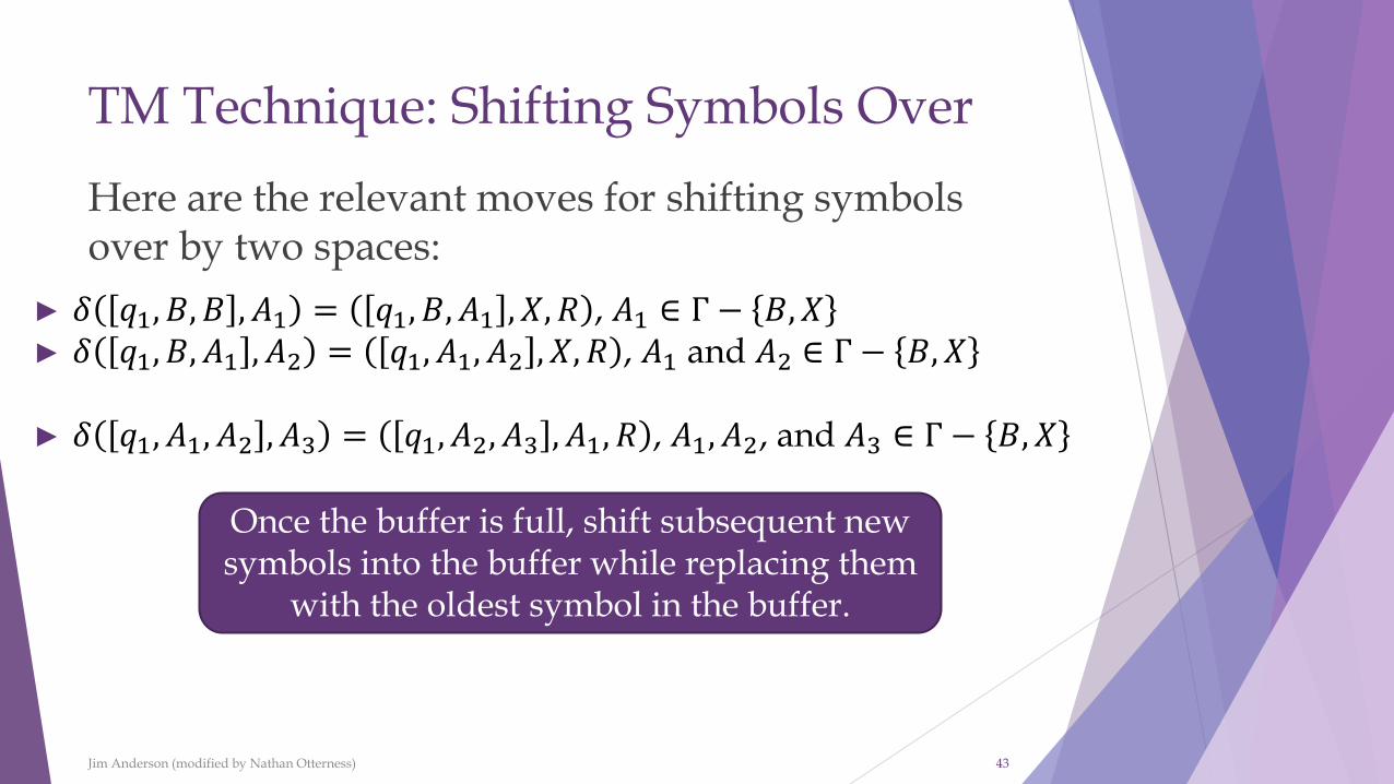
TM Technique: Shifting Symbols Over
Here are the relevant moves for shifting symbols over by two spaces:
Jim Anderson (modified by Nathan Otterness) 41
► 𝛿 𝑞1, 𝐵, 𝐵 , 𝐴1 = 𝑞1, 𝐵, 𝐴1 , 𝑋, 𝑅 , 𝐴1 ∈ Γ − 𝐵, 𝑋► 𝛿 𝑞1, 𝐵, 𝐴1 , 𝐴2 = 𝑞1, 𝐴1, 𝐴2 , 𝑋, 𝑅 , 𝐴1 and 𝐴2 ∈ Γ − 𝐵, 𝑋
► 𝛿 𝑞1, 𝐴1, 𝐴2 , 𝐴3 = 𝑞1, 𝐴2, 𝐴3 , 𝐴1, 𝑅 , 𝐴1, 𝐴2, and 𝐴3 ∈ Γ − 𝐵, 𝑋
► 𝛿 𝑞1, 𝐴1, 𝐴2 , 𝐵 = 𝑞1, 𝐴2, 𝐵 , 𝐴1, 𝑅 , 𝐴1 and 𝐴2 ∈ Γ − 𝐵, 𝑋► 𝛿 𝑞1, 𝐴1, 𝐵 , 𝐵 = 𝑞2, 𝐵, 𝐵 , 𝐴1, 𝐿 , 𝐴1 ∈ Γ − 𝐵, 𝑋
► 𝛿 𝑞2, 𝐵, 𝐵 , 𝐴 = 𝑞2, 𝐵, 𝐵 , 𝐴, 𝐿 , 𝐴 ∈ Γ − 𝐵, 𝑋

TM Technique: Shifting Symbols Over
Here are the relevant moves for shifting symbols over by two spaces:
Jim Anderson (modified by Nathan Otterness) 42
► 𝛿 𝑞1, 𝐵, 𝐵 , 𝐴1 = 𝑞1, 𝐵, 𝐴1 , 𝑋, 𝑅 , 𝐴1 ∈ Γ − 𝐵, 𝑋► 𝛿 𝑞1, 𝐵, 𝐴1 , 𝐴2 = 𝑞1, 𝐴1, 𝐴2 , 𝑋, 𝑅 , 𝐴1 and 𝐴2 ∈ Γ − 𝐵, 𝑋
Start by “shifting” the tape symbols 𝐴1 and 𝐴2 into the
finite-control buffer.
We will write the symbol 𝑋 into the “extra space” we are adding.
𝐴1 and 𝐴2 can’t be 𝐵. For simplicity, also assume that they can’t be 𝑋.
TM Technique: Shifting Symbols Over
Here are the relevant moves for shifting symbols over by two spaces:
Jim Anderson (modified by Nathan Otterness) 43
► 𝛿 𝑞1, 𝐵, 𝐵 , 𝐴1 = 𝑞1, 𝐵, 𝐴1 , 𝑋, 𝑅 , 𝐴1 ∈ Γ − 𝐵, 𝑋► 𝛿 𝑞1, 𝐵, 𝐴1 , 𝐴2 = 𝑞1, 𝐴1, 𝐴2 , 𝑋, 𝑅 , 𝐴1 and 𝐴2 ∈ Γ − 𝐵, 𝑋
► 𝛿 𝑞1, 𝐴1, 𝐴2 , 𝐴3 = 𝑞1, 𝐴2, 𝐴3 , 𝐴1, 𝑅 , 𝐴1, 𝐴2, and 𝐴3 ∈ Γ − 𝐵, 𝑋
Once the buffer is full, shift subsequent new symbols into the buffer while replacing them
with the oldest symbol in the buffer.
TM Technique: Shifting Symbols Over
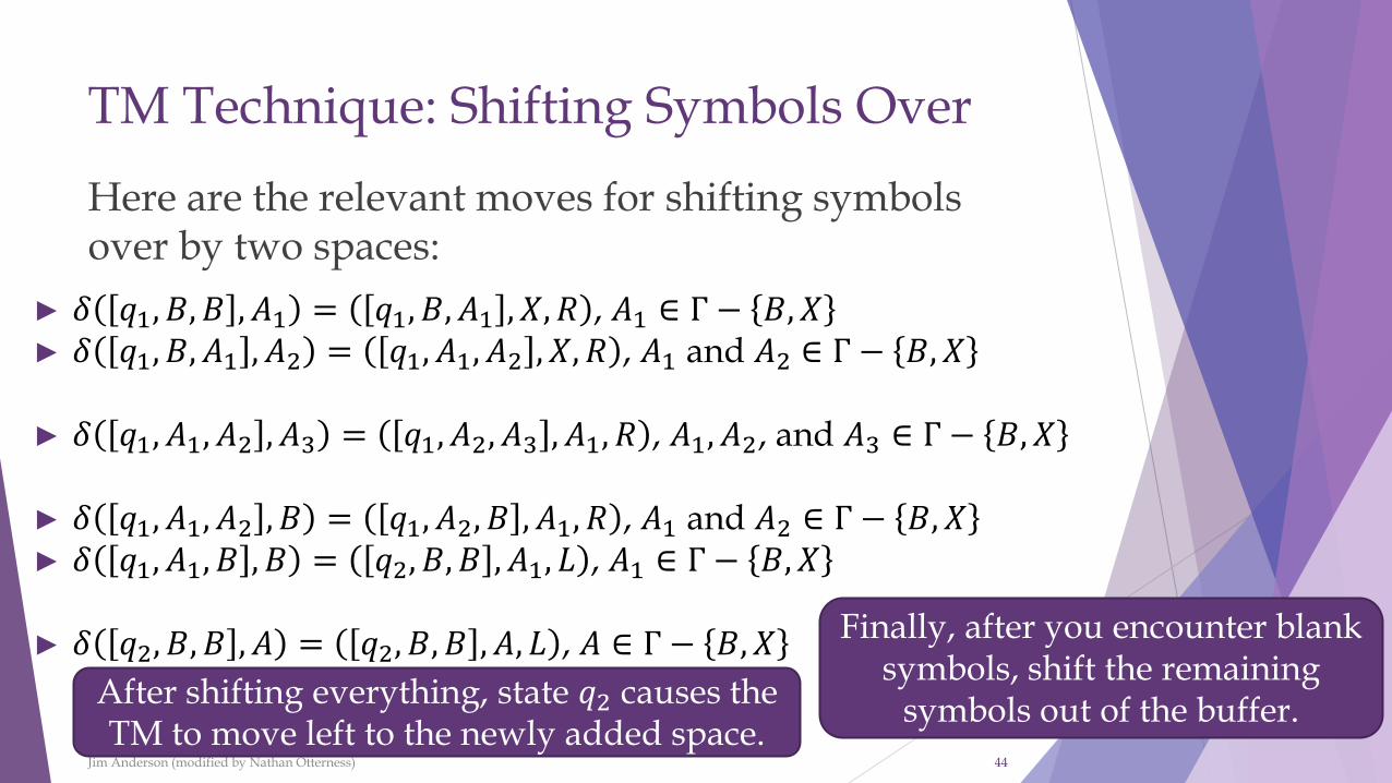
Here are the relevant moves for shifting symbols over by two spaces:
Jim Anderson (modified by Nathan Otterness) 44
► 𝛿 𝑞1, 𝐵, 𝐵 , 𝐴1 = 𝑞1, 𝐵, 𝐴1 , 𝑋, 𝑅 , 𝐴1 ∈ Γ − 𝐵, 𝑋► 𝛿 𝑞1, 𝐵, 𝐴1 , 𝐴2 = 𝑞1, 𝐴1, 𝐴2 , 𝑋, 𝑅 , 𝐴1 and 𝐴2 ∈ Γ − 𝐵, 𝑋
► 𝛿 𝑞1, 𝐴1, 𝐴2 , 𝐴3 = 𝑞1, 𝐴2, 𝐴3 , 𝐴1, 𝑅 , 𝐴1, 𝐴2, and 𝐴3 ∈ Γ − 𝐵, 𝑋
► 𝛿 𝑞1, 𝐴1, 𝐴2 , 𝐵 = 𝑞1, 𝐴2, 𝐵 , 𝐴1, 𝑅 , 𝐴1 and 𝐴2 ∈ Γ − 𝐵, 𝑋► 𝛿 𝑞1, 𝐴1, 𝐵 , 𝐵 = 𝑞2, 𝐵, 𝐵 , 𝐴1, 𝐿 , 𝐴1 ∈ Γ − 𝐵, 𝑋
► 𝛿 𝑞2, 𝐵, 𝐵 , 𝐴 = 𝑞2, 𝐵, 𝐵 , 𝐴, 𝐿 , 𝐴 ∈ Γ − 𝐵, 𝑋 Finally, after you encounter blank symbols, shift the remaining
symbols out of the buffer.After shifting everything, state 𝑞2 causes the TM to move left to the newly added space.
TM Technique: Shifting Symbols Over
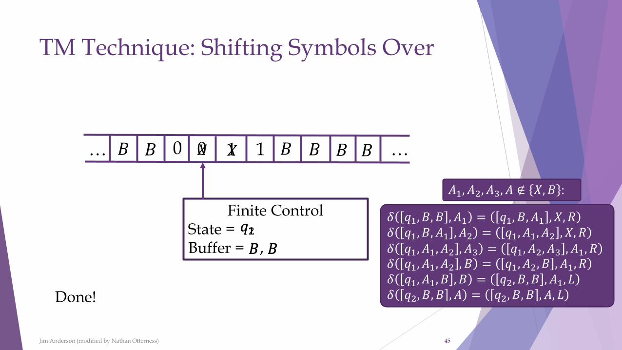
Jim Anderson (modified by Nathan Otterness) 45
0𝐵𝐵… 𝐵𝐵 …
Finite ControlState =Buffer = ,
0 1 1 𝐵
𝑞1𝐵 𝐵𝐵
𝑋 𝑋 𝐵
𝐵
𝑞2𝛿 𝑞1, 𝐵, 𝐵 , 𝐴1 = 𝑞1, 𝐵, 𝐴1 , 𝑋, 𝑅𝛿 𝑞1, 𝐵, 𝐴1 , 𝐴2 = 𝑞1, 𝐴1, 𝐴2 , 𝑋, 𝑅𝛿 𝑞1, 𝐴1, 𝐴2 , 𝐴3 = 𝑞1, 𝐴2, 𝐴3 , 𝐴1, 𝑅𝛿 𝑞1, 𝐴1, 𝐴2 , 𝐵 = 𝑞1, 𝐴2, 𝐵 , 𝐴1, 𝑅𝛿 𝑞1, 𝐴1, 𝐵 , 𝐵 = 𝑞2, 𝐵, 𝐵 , 𝐴1, 𝐿𝛿 𝑞2, 𝐵, 𝐵 , 𝐴 = 𝑞2, 𝐵, 𝐵 , 𝐴, 𝐿
𝐴1, 𝐴2, 𝐴3, 𝐴 ∉ 𝑋, 𝐵 :
Done!
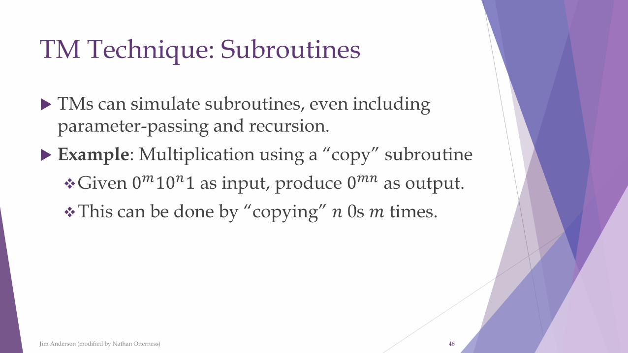
TM Technique: Subroutines
TMs can simulate subroutines, even including parameter-passing and recursion.
Example: Multiplication using a “copy” subroutine
❖Given 0𝑚10𝑛1 as input, produce 0𝑚𝑛 as output.
❖This can be done by “copying” 𝑛 0s 𝑚 times.
Jim Anderson (modified by Nathan Otterness) 46
TM Technique: Subroutines
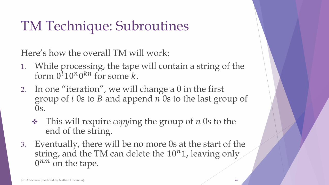
Here’s how the overall TM will work:
1. While processing, the tape will contain a string of the form 0𝑖10𝑛0𝑘𝑛 for some 𝑘.
2. In one “iteration”, we will change a 0 in the first group of 𝑖 0s to 𝐵 and append 𝑛 0s to the last group of 0s.
❖ This will require copying the group of 𝑛 0s to the end of the string.
3. Eventually, there will be no more 0s at the start of the string, and the TM can delete the 10𝑛1, leaving only 0𝑛𝑚 on the tape.
Jim Anderson (modified by Nathan Otterness) 47
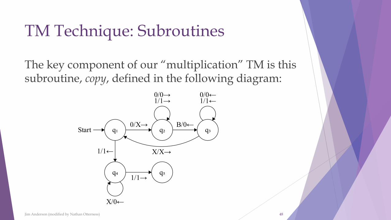
TM Technique: Subroutines
The key component of our “multiplication” TM is this subroutine, copy, defined in the following diagram:
Jim Anderson (modified by Nathan Otterness) 48
TM Technique: Subroutines
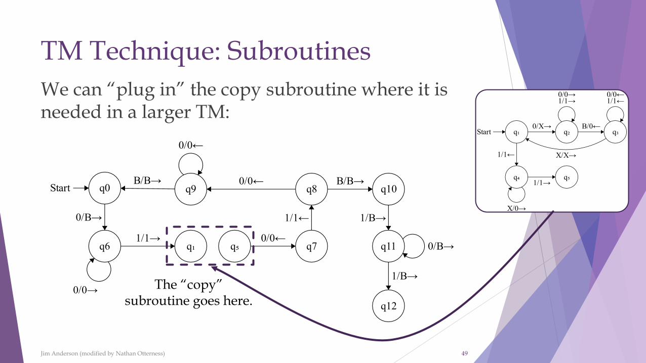
We can “plug in” the copy subroutine where it is needed in a larger TM:
Jim Anderson (modified by Nathan Otterness) 49
The “copy” subroutine goes here.
TM Technique: Subroutines
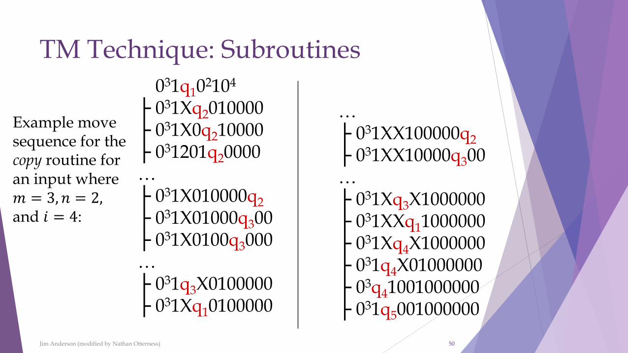
Jim Anderson (modified by Nathan Otterness) 50
031q102104
├ 031Xq2010000├ 031X0q210000├ 031201q20000…├ 031X010000q2
├ 031X01000q300├ 031X0100q3000…├ 031q3X0100000├ 031Xq10100000
…├ 031XX100000q2
├ 031XX10000q300…├ 031Xq3X1000000├ 031XXq11000000├ 031Xq4X1000000├ 031q4X01000000├ 03q41001000000├ 031q5001000000
Example move sequence for the copy routine for an input where 𝑚 = 3, 𝑛 = 2,and 𝑖 = 4:
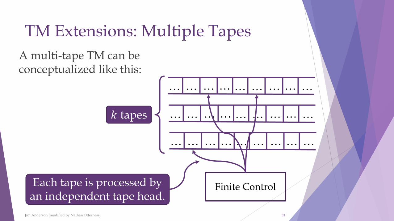
TM Extensions: Multiple Tapes
A multi-tape TM can be conceptualized like this:
Jim Anderson (modified by Nathan Otterness) 51
… …
Finite Control
… … …… … … …
… … … … …… … … …
… … … … …… … … …
𝑘 tapes
Each tape is processed by an independent tape head.
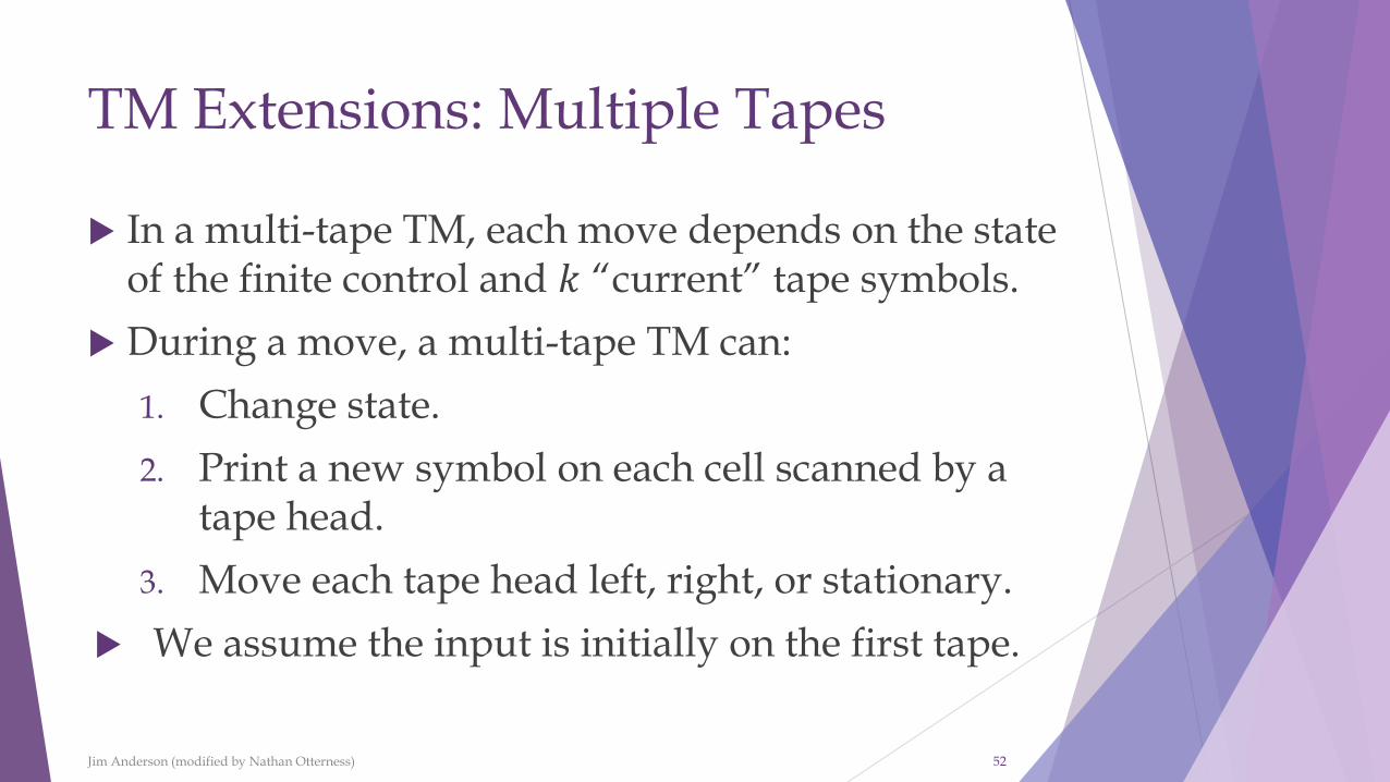
TM Extensions: Multiple Tapes
In a multi-tape TM, each move depends on the state of the finite control and 𝑘 “current” tape symbols.
During a move, a multi-tape TM can:
1. Change state.
2. Print a new symbol on each cell scanned by a tape head.
3. Move each tape head left, right, or stationary.
We assume the input is initially on the first tape.
Jim Anderson (modified by Nathan Otterness) 52
Single-Tape vs. Multi-Tape TMs
Theorem 8.9: If 𝐿 is accepted by a multi-tape TM, then it is accepted by a single-tape TM.
Proof:
Let 𝑀 be a multi-tape TM with 𝑘 tapes.
We can construct a single-tape TM, 𝑀′ with 2𝑘tracks that accepts 𝐿 𝑀 .
Jim Anderson (modified by Nathan Otterness) 53
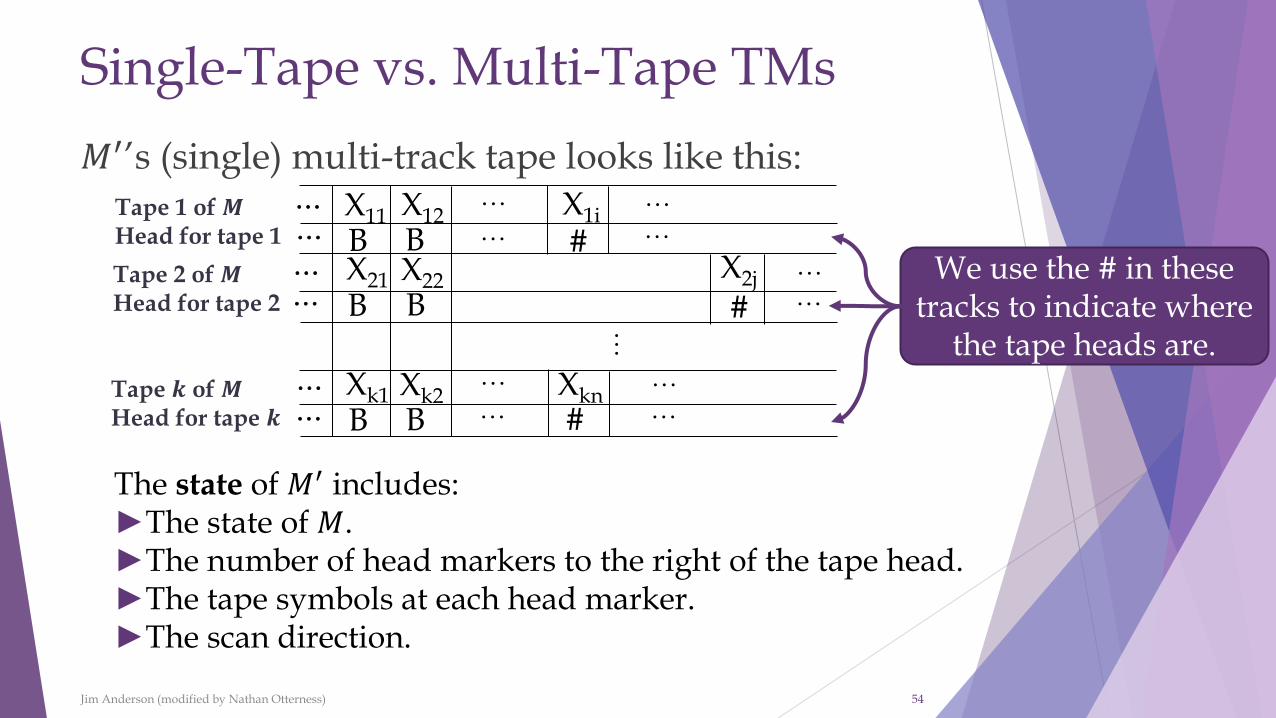
Single-Tape vs. Multi-Tape TMs
𝑀′’s (single) multi-track tape looks like this:
Jim Anderson (modified by Nathan Otterness) 54
X11 X12 X1i
X2jX22X21
Xk1 Xk2 Xkn
B B #
B B
B B #
#
Tape 1 of 𝑴Head for tape 1
Tape 2 of 𝑴Head for tape 2
Tape 𝒌 of 𝑴Head for tape 𝒌
The state of 𝑀′ includes:►The state of 𝑀.►The number of head markers to the right of the tape head.►The tape symbols at each head marker.►The scan direction.
We use the # in these tracks to indicate where
the tape heads are.
Single-Tape vs. Multi-Tape TMs
Jim Anderson (modified by Nathan Otterness) 55
X11 X12 X1i
X2jX22X21
Xk1 Xk2 Xkn
B B #
B B
B B #
#
Tape 1 of 𝑴Head for tape 1
Tape 2 of 𝑴Head for tape 2
Tape 𝒌 of 𝑴Head for tape 𝒌
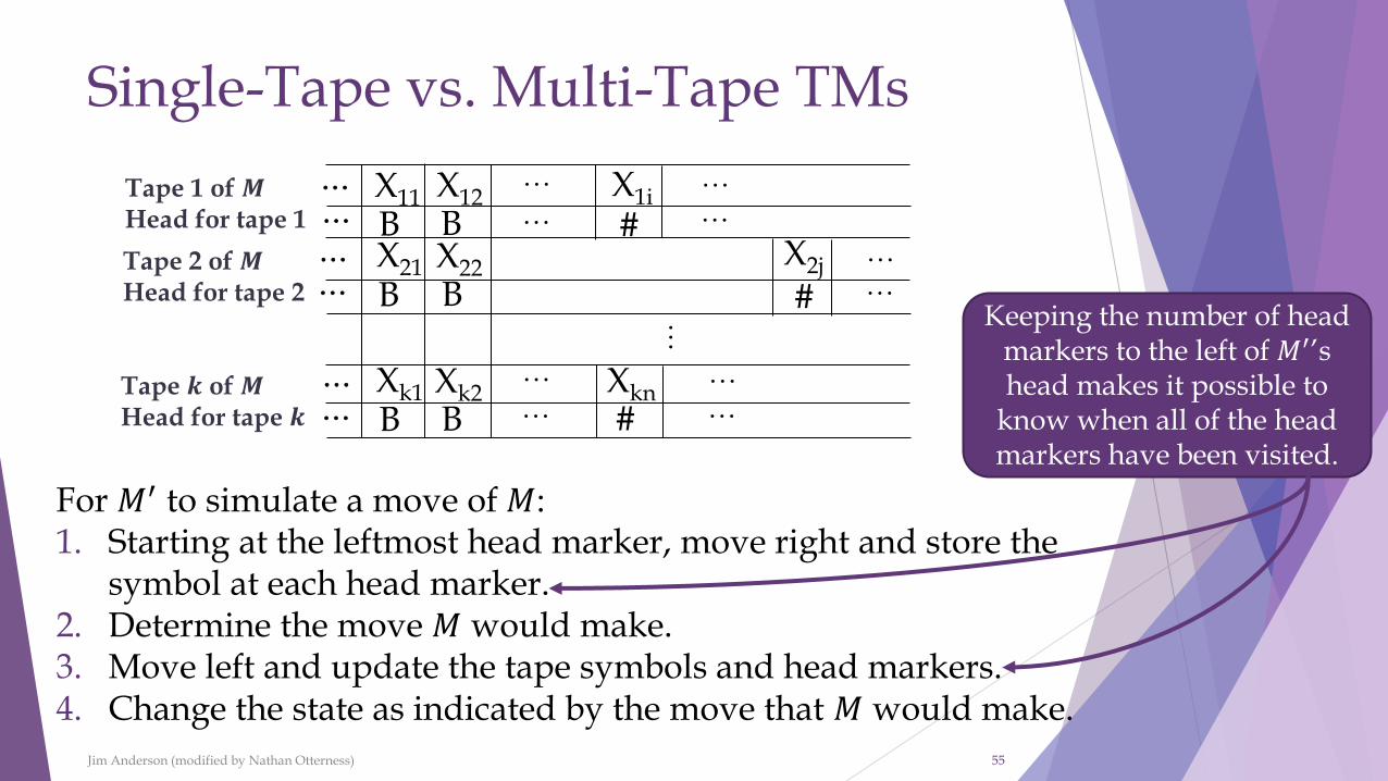
For 𝑀′ to simulate a move of 𝑀:1. Starting at the leftmost head marker, move right and store the
symbol at each head marker.2. Determine the move 𝑀 would make.3. Move left and update the tape symbols and head markers.4. Change the state as indicated by the move that 𝑀 would make.
Keeping the number of head markers to the left of 𝑀′’s head makes it possible to
know when all of the head markers have been visited.
Single-Tape vs. Multi-Tape TMs
Jim Anderson (modified by Nathan Otterness) 56
X11 X12 X1i
X2jX22X21
Xk1 Xk2 Xkn
B B #
B B
B B #
#
Tape 1 of 𝑴Head for tape 1
Tape 2 of 𝑴Head for tape 2
Tape 𝒌 of 𝑴Head for tape 𝒌
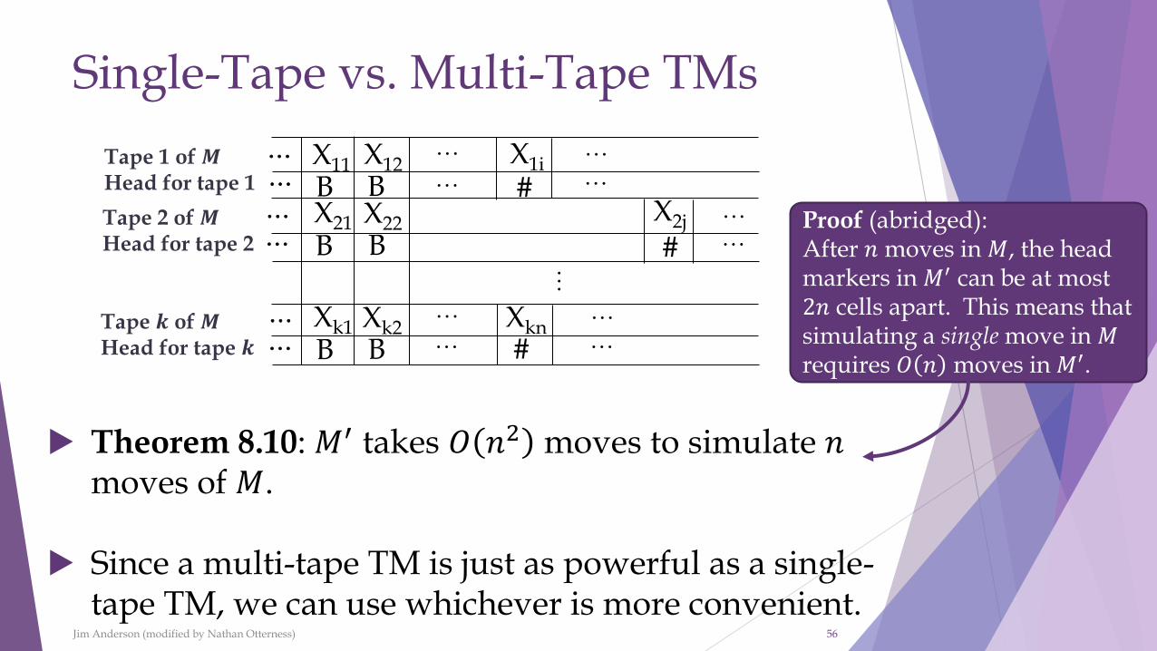
▶ Theorem 8.10: 𝑀′ takes 𝑂 𝑛2 moves to simulate 𝑛moves of 𝑀.
▶ Since a multi-tape TM is just as powerful as a single-tape TM, we can use whichever is more convenient.
Proof (abridged):After 𝑛 moves in 𝑀, the head markers in 𝑀′ can be at most 2𝑛 cells apart. This means that simulating a single move in 𝑀requires 𝑂 𝑛 moves in 𝑀′.
TM Extensions: Nondeterministic TMs
The original definition we discussed was for a deterministic TM (DTM).
A nondeterministic TM (NDTM) can “choose” between multiple possible moves for any combination of state and tape symbol(s).
Move function for a nondeterministic TM with 𝑘 tapes:
❖𝛿 maps 𝑄 × Γ𝑘 to subsets of 𝑄 × Γ × 𝐿, 𝑅, 𝑆 𝑘.
Jim Anderson (modified by Nathan Otterness) 57
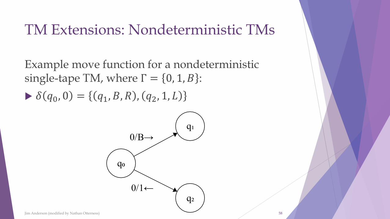
TM Extensions: Nondeterministic TMs
Example move function for a nondeterministic single-tape TM, where Γ = 0, 1, 𝐵 :
𝛿 𝑞0, 0 = 𝑞1, 𝐵, 𝑅 , 𝑞2, 1, 𝐿
Jim Anderson (modified by Nathan Otterness) 58
Nondeterministic TMs
Theorem 8.11: If 𝐿 is accepted by a single-tape NDTM 𝑀1, then 𝐿 is accepted by some DTM 𝑀2.
Let 𝑑 be the maximum number of nondeterministic choices 𝑀1 can make at any given move.
𝑀2 will systematically try all nondeterministic possibilities.
𝑀2 will have three tapes.
Jim Anderson (modified by Nathan Otterness) 59
Note: The book reasons about a multi-tape
NDTM here, instead.
Nondeterministic TMs
How 𝑀2 works:
Tape 1 holds the input.
Tape 2 contains a sequence of digits from 1 to 𝑑, generated systematically. Each sequence dictates a sequence of choices. e.g.,
❖ 1 , 2 , 3 , … , 𝑑 ,1,1 , 1, 2 , 2, 1 , … , 𝑑, 𝑑 ,1,1,1 , 1,1,2 , 1, 2, 1 , … , 𝑑, 𝑑, 𝑑 ,
…
Tape 3 contains a scratch copy of the input.
Jim Anderson (modified by Nathan Otterness) 60
Nondeterministic TMs
How 𝑀2 works (continued):
1. Generate the next sequence on tape 2
2. Copy tape 1 (input) to tape 3 (scratch copy)
3. Simulate 𝑀1 on tape 3, making choices according to the sequence on tape 2.
4. If 𝑀1 accepts, then accept;
5. Otherwise, go to step 1.
Jim Anderson (modified by Nathan Otterness) 61
Nondeterminism and Time Complexity
Definition: A NDTM 𝑀 is of time complexity 𝑇 𝑛 if for every accepted string of length 𝑛, some sequence of at most 𝑇 𝑛 moves leading to an accepting state exists.
Theorem: If 𝐿 is accepted by a single-tape NDTM 𝑀1
with time complexity 𝑇 𝑛 , then 𝐿 is accepted by some
DTM 𝑀2 with time complexity 𝑂 𝑐𝑇 𝑛 , for some constant 𝑐.
Proof: If 𝑀1 in the previous construction can accept in at most 𝑇 𝑛 moves, then 𝑀2 can accept in at most
𝑂 𝑇 𝑛 𝑑 + 1 𝑇 𝑛 moves.Jim Anderson (modified by Nathan Otterness) 62
Restricted TMs: Semi-infinite Tape
In a TM with a semi-infinite tape, the tape is infinite only to the right of the starting position.
❖Assume that trying to move left from the leftmost cell causes execution to die.
Theorem 8.12: (reworded) 𝐿 is recognized by a TM with a two-way infinite tape if and only if it is recognized by a TM with a semi-infinite tape.
Jim Anderson (modified by Nathan Otterness) 63
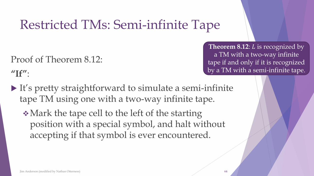
Restricted TMs: Semi-infinite Tape
Proof of Theorem 8.12:
“If”:
It’s pretty straightforward to simulate a semi-infinite tape TM using one with a two-way infinite tape.
❖Mark the tape cell to the left of the starting position with a special symbol, and halt without accepting if that symbol is ever encountered.
Jim Anderson (modified by Nathan Otterness) 64
Theorem 8.12: 𝐿 is recognized by a TM with a two-way infinite
tape if and only if it is recognized by a TM with a semi-infinite tape.
Restricted TMs: Semi-infinite Tape
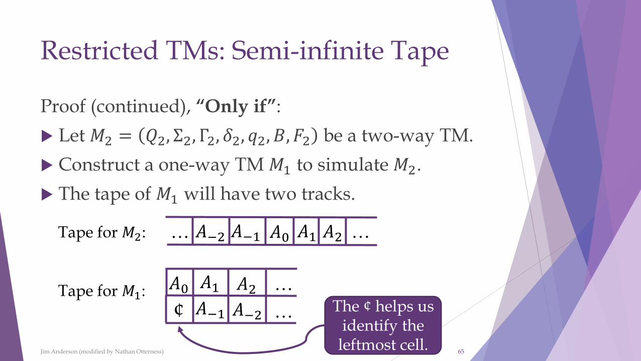
Proof (continued), “Only if”:
Let 𝑀2 = 𝑄2, Σ2, Γ2, 𝛿2, 𝑞2, 𝐵, 𝐹2 be a two-way TM.
Construct a one-way TM 𝑀1 to simulate 𝑀2.
The tape of 𝑀1 will have two tracks.
Jim Anderson (modified by Nathan Otterness) 65
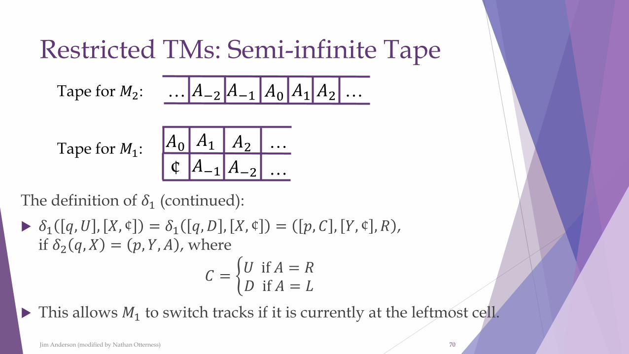
… 𝐴−2 𝐴−1 𝐴0 𝐴1 𝐴2 …
𝐴0 𝐴1 𝐴2 …
𝐴−1 𝐴−2 …¢
Tape for 𝑀2:
Tape for 𝑀1:The ¢ helps us
identify the leftmost cell.
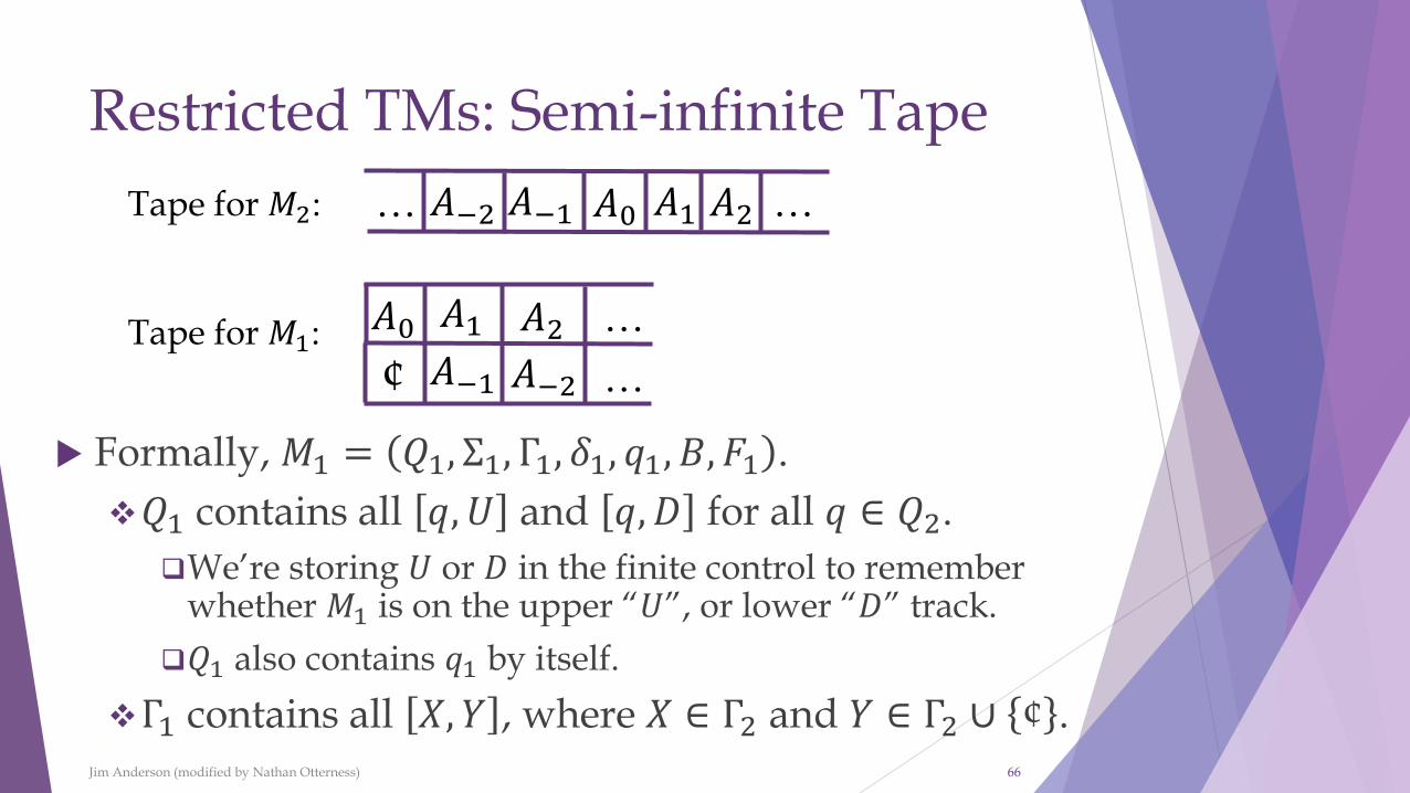
Restricted TMs: Semi-infinite Tape
Formally, 𝑀1 = 𝑄1, Σ1, Γ1, 𝛿1, 𝑞1, 𝐵, 𝐹1 .
❖𝑄1 contains all 𝑞, 𝑈 and 𝑞, 𝐷 for all 𝑞 ∈ 𝑄2.
❑We’re storing 𝑈 or 𝐷 in the finite control to remember whether 𝑀1 is on the upper “𝑈”, or lower “𝐷” track.
❑𝑄1 also contains 𝑞1 by itself.
❖Γ1 contains all 𝑋, 𝑌 , where 𝑋 ∈ Γ2 and 𝑌 ∈ Γ2 ∪ ¢ .Jim Anderson (modified by Nathan Otterness) 66
… 𝐴−2 𝐴−1 𝐴0 𝐴1 𝐴2 …
𝐴0 𝐴1 𝐴2 …
𝐴−1 𝐴−2 …¢
Tape for 𝑀2:
Tape for 𝑀1:
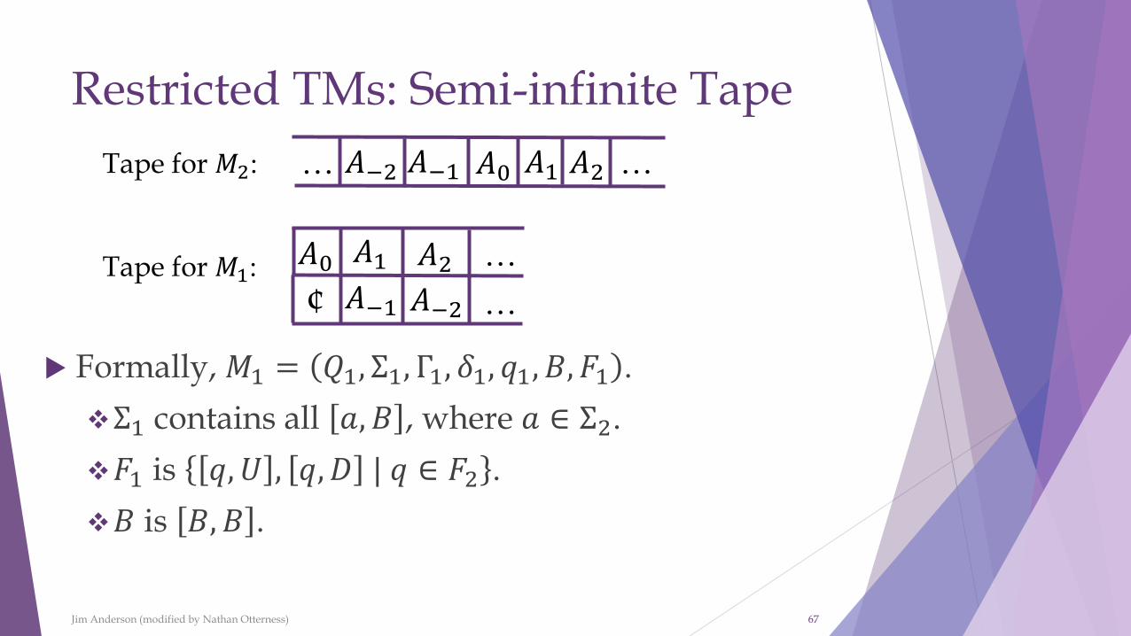
Restricted TMs: Semi-infinite Tape
Formally, 𝑀1 = 𝑄1, Σ1, Γ1, 𝛿1, 𝑞1, 𝐵, 𝐹1 .
❖Σ1 contains all 𝑎, 𝐵 , where 𝑎 ∈ Σ2.
❖𝐹1 is 𝑞, 𝑈 , 𝑞, 𝐷 | 𝑞 ∈ 𝐹2 .
❖𝐵 is 𝐵, 𝐵 .
Jim Anderson (modified by Nathan Otterness) 67
… 𝐴−2 𝐴−1 𝐴0 𝐴1 𝐴2 …
𝐴0 𝐴1 𝐴2 …
𝐴−1 𝐴−2 …¢
Tape for 𝑀2:
Tape for 𝑀1:

Restricted TMs: Semi-infinite Tape
The definition of 𝛿1:
𝛿1 𝑞1, 𝑎, 𝐵 = 𝑞, 𝑈 , 𝑋, ¢ , 𝑅 if 𝛿2 𝑞2, 𝑎 = 𝑞, 𝑋, 𝑅
❖This is the case when the first move of 𝑀2 is right.
𝛿1 𝑞1, 𝑎, 𝐵 = 𝑞, 𝐷 , 𝑋, ¢ , 𝑅 if 𝛿2 𝑞2, 𝑎 = 𝑞, 𝑋, 𝐿
❖This is the case when the first move of 𝑀2 is left.Jim Anderson (modified by Nathan Otterness) 68
… 𝐴−2 𝐴−1 𝐴0 𝐴1 𝐴2 …
𝐴0 𝐴1 𝐴2 …
𝐴−1 𝐴−2 …¢
Tape for 𝑀2:
Tape for 𝑀1:
Restricted TMs: Semi-infinite Tape
The definition of 𝛿1 (continued):
For all 𝑋, 𝑌 ∈ Γ1, with 𝑌 ≠ ¢, and 𝐴 = 𝐿 or 𝑅:
𝛿1 𝑞, 𝑈 , 𝑋, 𝑌 = 𝑝, 𝑈 , 𝑍, 𝑌 , 𝐴 if 𝛿2 𝑞, 𝑋 = 𝑝, 𝑍, 𝐴 .
❖ This simulates 𝑀2 on the upper track.
𝛿1 𝑞, 𝐷 , 𝑋, 𝑌 = 𝑝, 𝐷 , 𝑋, 𝑍 , 𝐴 if 𝛿2 𝑞, 𝑌 = 𝑝, 𝑍, ҧ𝐴
❖ This simulates 𝑀2 on the lower track.
Jim Anderson (modified by Nathan Otterness) 69
… 𝐴−2 𝐴−1 𝐴0 𝐴1 𝐴2 …
𝐴0 𝐴1 𝐴2 …
𝐴−1 𝐴−2 …¢
Tape for 𝑀2:
Tape for 𝑀1:
If we’re in the lower track in 𝑀1 we need to move in the opposite direction from
how 𝑀2 would move.
Restricted TMs: Semi-infinite Tape
The definition of 𝛿1 (continued):
𝛿1 𝑞, 𝑈 , 𝑋, ¢ = 𝛿1 𝑞, 𝐷 , 𝑋, ¢ = 𝑝, 𝐶 , 𝑌, ¢ , 𝑅 ,if 𝛿2 𝑞, 𝑋 = 𝑝, 𝑌, 𝐴 , where
𝐶 = ቊ𝑈 if 𝐴 = 𝑅𝐷 if 𝐴 = 𝐿
This allows 𝑀1 to switch tracks if it is currently at the leftmost cell.
Jim Anderson (modified by Nathan Otterness) 70
… 𝐴−2 𝐴−1 𝐴0 𝐴1 𝐴2 …
𝐴0 𝐴1 𝐴2 …
𝐴−1 𝐴−2 …¢
Tape for 𝑀2:
Tape for 𝑀1:
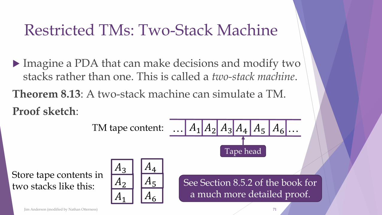
Restricted TMs: Two-Stack Machine
Imagine a PDA that can make decisions and modify two stacks rather than one. This is called a two-stack machine.
Theorem 8.13: A two-stack machine can simulate a TM.
Proof sketch:
Jim Anderson (modified by Nathan Otterness) 71
… …𝐴2𝐴1 𝐴4𝐴3 𝐴5 𝐴6
See Section 8.5.2 of the book for a much more detailed proof.
Tape head
Store tape contents in two stacks like this:
𝐴1
𝐴2
𝐴3
𝐴6
𝐴5
𝐴4
TM tape content:
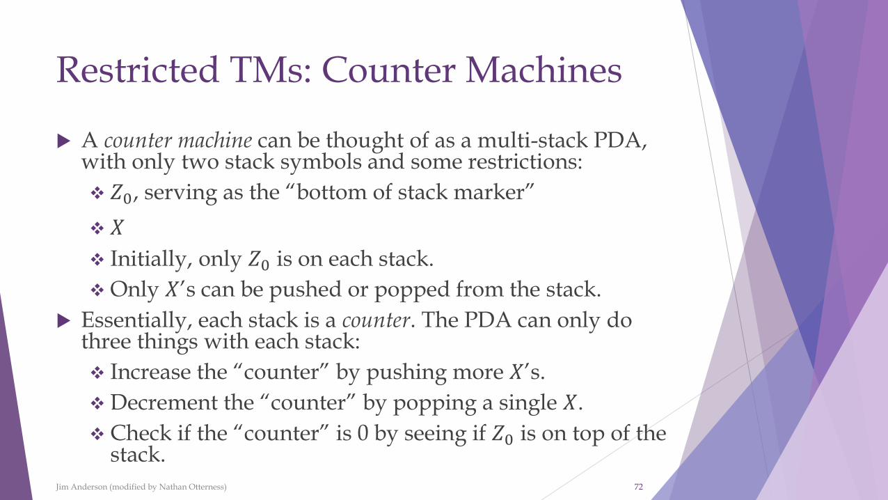
Restricted TMs: Counter Machines
A counter machine can be thought of as a multi-stack PDA, with only two stack symbols and some restrictions:
❖ 𝑍0, serving as the “bottom of stack marker”
❖ 𝑋
❖ Initially, only 𝑍0 is on each stack.
❖ Only 𝑋’s can be pushed or popped from the stack.
Essentially, each stack is a counter. The PDA can only do three things with each stack:
❖ Increase the “counter” by pushing more 𝑋’s.
❖ Decrement the “counter” by popping a single 𝑋.
❖ Check if the “counter” is 0 by seeing if 𝑍0 is on top of the stack.
Jim Anderson (modified by Nathan Otterness) 72

Restricted TMs: Three-Counter Machines
Theorem 8.14: Every RE language is accepted by a three-counter machine.
Proof:
We will show that one stack can be simulated by two counters, the second of which is a “scratch” counter used for calculations.
When simulating two stacks, we can then use the same scratch counter, so three counters in total are sufficient.
Jim Anderson (modified by Nathan Otterness) 73
Restricted TMs: Three-Counter Machines
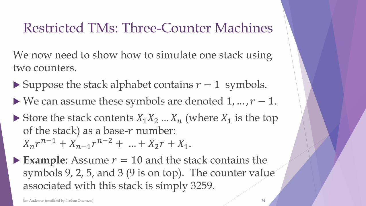
We now need to show how to simulate one stack using two counters.
Suppose the stack alphabet contains 𝑟 − 1 symbols.
We can assume these symbols are denoted 1,… , 𝑟 − 1.
Store the stack contents 𝑋1𝑋2…𝑋𝑛 (where 𝑋1 is the top of the stack) as a base-𝑟 number:𝑋𝑛𝑟
𝑛−1 + 𝑋𝑛−1𝑟𝑛−2 + …+ 𝑋2𝑟 + 𝑋1.
Example: Assume 𝑟 = 10 and the stack contains the symbols 9, 2, 5, and 3 (9 is on top). The counter value associated with this stack is simply 3259.Jim Anderson (modified by Nathan Otterness) 74

Restricted TMs: Three-Counter Machines
We now need to show how to simulate stack operations using a counter.
Pop the stack: Replace the counter value 𝑖 by 𝑖/𝑟. The remainder is the old top-of-stack symbol, which can be stored in the finite control.
❖Example: popping 3259. 3259
𝑟=
3259
10= 325, with
remainder 9.
Jim Anderson (modified by Nathan Otterness) 75
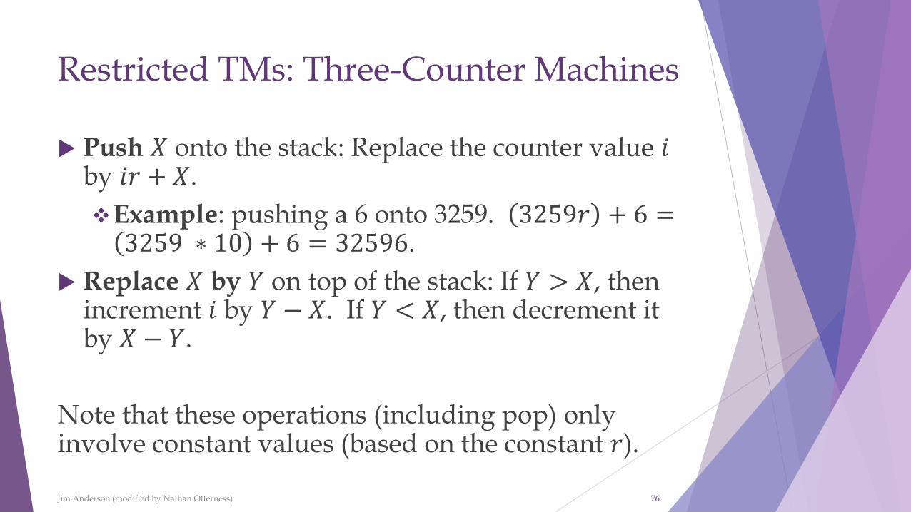
Restricted TMs: Three-Counter Machines
Push 𝑋 onto the stack: Replace the counter value 𝑖by 𝑖𝑟 + 𝑋.
❖Example: pushing a 6 onto 3259. 3259𝑟 + 6 =3259 ∗ 10 + 6 = 32596.
Replace 𝑋 by 𝑌 on top of the stack: If 𝑌 > 𝑋, then increment 𝑖 by 𝑌 − 𝑋. If 𝑌 < 𝑋, then decrement it by 𝑋 − 𝑌.
Note that these operations (including pop) only involve constant values (based on the constant 𝑟).
Jim Anderson (modified by Nathan Otterness) 76
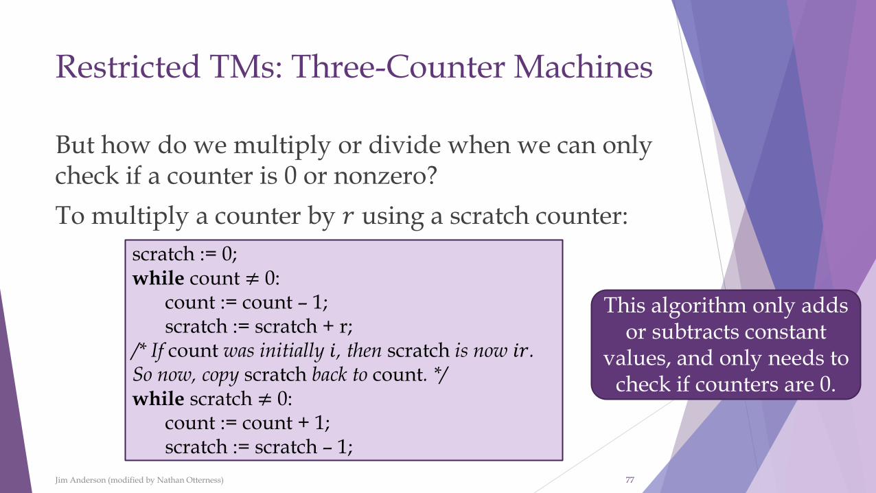
Restricted TMs: Three-Counter Machines
But how do we multiply or divide when we can only check if a counter is 0 or nonzero?
To multiply a counter by 𝑟 using a scratch counter:
Jim Anderson (modified by Nathan Otterness) 77
scratch := 0;while count ≠ 0:
count := count – 1;scratch := scratch + r;
/* If count was initially 𝑖, then scratch is now 𝑖𝑟. So now, copy scratch back to count. */while scratch ≠ 0:
count := count + 1;scratch := scratch – 1;
This algorithm only adds or subtracts constant
values, and only needs to check if counters are 0.
Restricted TMs: Three-Counter Machines
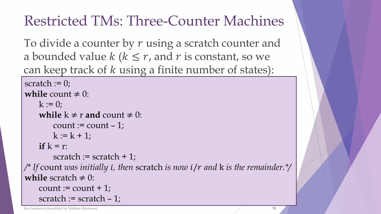
To divide a counter by 𝑟 using a scratch counter and a bounded value 𝑘 (𝑘 ≤ 𝑟, and 𝑟 is constant, so we can keep track of 𝑘 using a finite number of states):
Jim Anderson (modified by Nathan Otterness) 78
scratch := 0;while count ≠ 0:
k := 0;while k ≠ r and count ≠ 0:
count := count – 1;k := k + 1;
if k = r:scratch := scratch + 1;
/* If count was initially 𝑖, then scratch is now 𝑖/𝑟 and k is the remainder.*/while scratch ≠ 0:
count := count + 1;scratch := scratch – 1;
Restricted TMs: Two-Counter Machines
We have now shown that we can simulate a single stack using two counters, and two stacks using three counters, but we can go farther!
Theorem 8.15: Every RE language is accepted by a two-counter machine.
Proof: We will show that we can simulate three counters using two counters.
If 𝑖, 𝑗, and 𝑘 are the three counts we want to track, we can store them in a single integer 𝑛 = 2𝑖3𝑗5𝑘.
Jim Anderson (modified by Nathan Otterness) 79

Restricted TMs: Two-Counter Machines
(From previous slide) If 𝑖, 𝑗, and 𝑘 are the three counts we want to track, we can store them in a single integer 𝑛 = 2𝑖3𝑗5𝑘.
To increment 𝑖: Replace 𝑛 by 2𝑛.
To decrement 𝑖: Replace 𝑛 by 𝑛/2.
To test if 𝑖 is 0: Check if 𝑛 is not divisible by 2.
The other counters are similar (e.g. increment 𝑗 by replacing 𝑛with 3𝑛 and increment 𝑘 by setting 𝑛 = 5𝑛, etc.).
We have already seen how to multiply and divide by constant values using a second “scratch” counter.
Note that this construction works because 2, 3, and 5 are relatively prime.
Jim Anderson (modified by Nathan Otterness) 80
Restricted TMs: Summary
We have shown that the following machines are equally powerful in terms of languages they can identify:
❖Nondeterministic TMs
❖Multi-tape TMs
❖Multi-track TMs
❖Single-tape TMs
❖Semi-infinite tape TMs
❖Two-stack machines
❖Three-counter machines
❖Two-counter machines
Jim Anderson (modified by Nathan Otterness) 81
TMs vs. “Real” Computers
We want to show that anything a TM can do is possible using a computer, and vice versa.
Designing a computer that simulates a TM is easy: just store the transition function in a table, which tells a program what to do next.
One “gotcha”: a TM has infinite memory.
❖ The book says we can just continually add new disks to a TM when old ones are full.
❖ What if we have TM that uses more tape cells than atoms in the universe? (Clearly the book’s approach isn’t a true Turing Machine.)
❖ My take: we can’t simulate infinite memory, but we will also never have a practical application that requires it.
Jim Anderson (modified by Nathan Otterness) 82
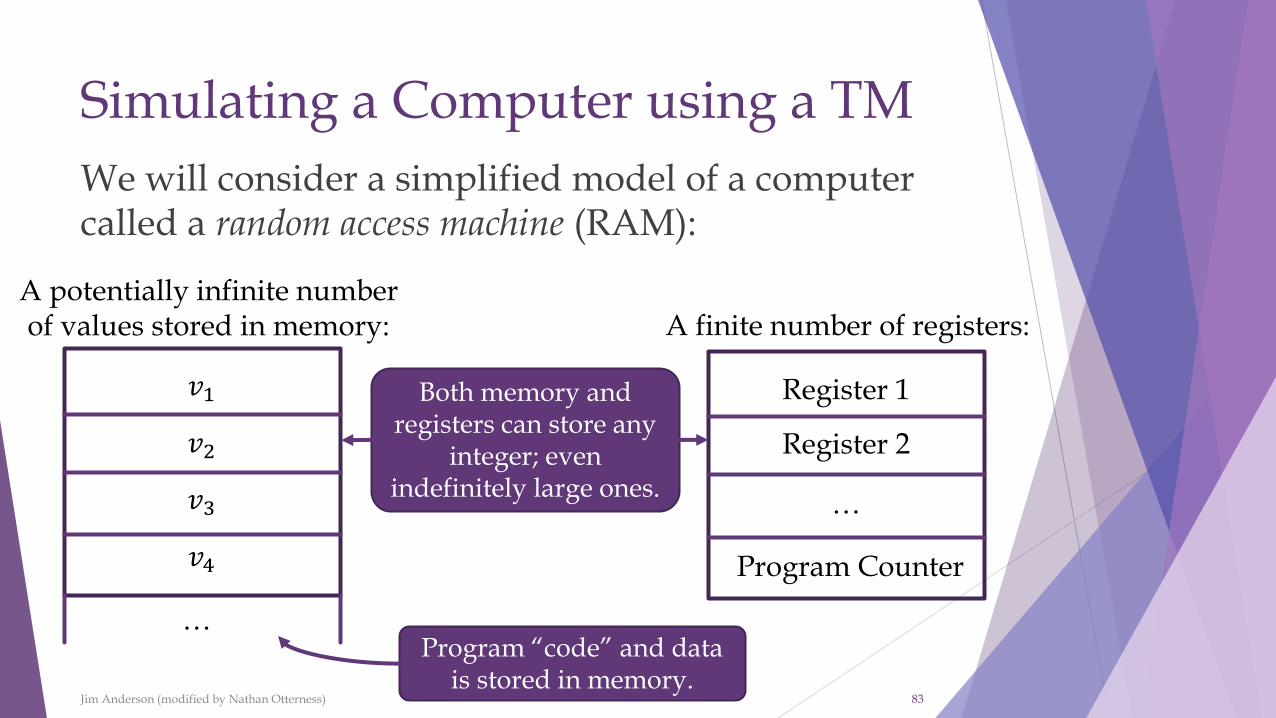
Simulating a Computer using a TM
We will consider a simplified model of a computer called a random access machine (RAM):
Jim Anderson (modified by Nathan Otterness) 83
A potentially infinite number of values stored in memory:
𝑣1
…
Register 1
Register 2
…
Program Counter
A finite number of registers:
Both memory and registers can store any
integer; even indefinitely large ones.
Program “code” and data is stored in memory.
𝑣2
𝑣3
𝑣4
Random Access Machines
In a RAM, a “program” is a list of instructions.
❖Instructions are like what you’d find on a “real” computer, and consist of an opcode and an address.
❖Instructions are encoded as a single integer (e.g. with some bits representing the opcode and the remaining bits representing the argument).
With this model, you can have basic instructions like LOAD, STORE, ADD, etc., like an assembly language.
Jim Anderson (modified by Nathan Otterness) 84
Simulating a Random Access Machine
Theorem: A TM can simulate a RAM, provided that the TM can simulate each individual RAM instruction.
For example, you can’t have a RAM instruction that solves the halting problem.
Proof sketch:
We will use multiple tapes to store the RAM’s memory and register values in a TM.
Jim Anderson (modified by Nathan Otterness) 85
Simulating a Random Access Machine
One tape in our TM holds memory values that have been written.
❖The format of this tape is #0*𝑣0#1*𝑣1#10*𝑣2#...
❖The # and * are simply delimiters around the “address” of each value. Assume that each 𝑣𝑖 is stored in binary.
Use one additional tape for each register.
Jim Anderson (modified by Nathan Otterness) 86
Simulating a Random Access Machine
Overview of the TM’s behavior for simulating the RAM:
1. Read the current PC value 𝑖 from the tape holding the “program counter” register.
2. Scan the memory tape for the “address” #𝑖*. Halt if it isn’t found.
3. Decode the instruction opcode and address from the memory value at location 𝑖.
4. Perform the operation indicated by the opcode and address.
5. Repeat from step 1.
Jim Anderson (modified by Nathan Otterness) 87
Simulating a Random Access Machine
Possible behavior for a couple common “instructions”:
If the instruction indicates to “ADD” a value at address 𝑗 to a register:
1. Scan memory for #𝑗*, and add the value found afterwards to a register.
2. Add 1 to the program counter register to advance to the next instruction.
If the instruction indicates to “GOTO” address 𝑗:
1. Copy the address 𝑗 to the program counter register.
(Other instructions can be simulated in a similar manner)
Jim Anderson (modified by Nathan Otterness) 88
Running Time of the RAM Simulation
The previous simulation will run in polynomial timeprovided that a couple restrictions hold:
First, the RAM can’t have an instruction that takes exponential time to compute.
❖For example, you can’t have a “solve the traveling salesman problem” instruction.
❖This isn’t a big restriction, because no real computer will have instructions like this anyway.
Jim Anderson (modified by Nathan Otterness) 89

Running Time of the RAM Simulation
(Continued list of restrictions for this simulation)
Second, we can’t have instructions that “drastically” increase the length of some number.
❖Example: If integer values are unrestricted, then starting with a value 2, applying a hypothetical “multiply a value by itself” instruction 𝑛 times would lead to a value of 22
𝑛,
which takes 2𝑛+1 bits to represent. Just writing these down takes exponential time, so we don’t allow instructions like this.
❖ In reality, this is also a mild restriction. In real computers, the lengths of individual numbers are limited.
Jim Anderson (modified by Nathan Otterness) 90
Running Time of the RAM Simulation
Theorem 8.17: If a computer has (1) only instructions that increase the length of a number by 1 bit and (2) has only instructions that a multi-tape TM can perform on numbers of length 𝑘 in 𝑂 𝑘2 steps, then a TM exists that can simulate 𝑛 steps of the computer in 𝑂 𝑛3 moves.
Notes:
(1) rules out multiplication, which can double the length of a number. However, multiplication can be simulated in polynomial time by repeatedly adding, which is allowed.
The 𝑂 𝑘2 bound in (2) was selected because it seems sufficient for most “reasonable” instructions.
Jim Anderson (modified by Nathan Otterness) 91
Running Time of the RAM Simulation
We won’t prove Theorem 8.17 in detail. However,
If individual instructions can be simulated in polynomial time, we only need to worry about spending an exponential amount of time scanning the “memory” tape.
Initially, the “memory” tape holds the program to execute and input data, all of which starts at a “constant” length.
Restriction (1) ensures that the tape’s length remains polynomial in 𝑛 (after executing 𝑛 RAM instructions). See book Section 8.6.3 for the proof.
Jim Anderson (modified by Nathan Otterness) 92

Final Comment on RAM Simulation
We know from before that a single-tape TM can simulate a multi-tape TM in polynomial time.
So, even a single-tape TM can simulate a RAM computation in polynomial time.
Jim Anderson (modified by Nathan Otterness) 93