Turbulent Boundary Layers & Turbulence Models€¦ · Turbulence models • A turbulence model is a...
45
Turbulent Boundary Layers & Turbulence Models Lecture 09
Transcript of Turbulent Boundary Layers & Turbulence Models€¦ · Turbulence models • A turbulence model is a...

Turbulent Boundary Layers &
Turbulence Models
Lecture 09

The turbulent boundary layer
• In turbulent flow, the boundary layer is defined as the thin region on the
surface of a body in which viscous effects are important.
• The boundary layer allows the fluid to transition from the free stream
velocity U to a velocity of zero at the wall.
• The velocity component normal to the surface is much smaller than the
velocity parallel to the surface: v << u.
• The gradients of the flow across the layer are much greater than the
gradients in the flow direction.
• The boundary layer thickness δ is defined as the distance away from the
surface where the velocity reaches 99% of the free-stream velocity.
= 0.99U
δ = y, where u

no separation
steady separation
unsteady vortex shedding
laminar BL
wide turbulent wake
turbulent BL
narrow turbulent wake
Drag on a smooth circular cylinder
• The drag coefficient is defined as follows:
Turbulent flow reduced drag

The turbulent boundary layer
The turbulent boundary layer
• Important variables:
– Distance from the wall: y.
– Wall shear stress: τw. The force exerted on a flat plate is the areatimes the wall shear stress.
– Density: ρ.
– Dynamic viscosity: µ.
– Kinematic viscosity: ν.
– Velocity at y: U.
– The friction velocity: uτ = (τw/ρ)1/2 .
• We can define a Reynolds number based on the distance to the
wall using the friction velocity: y+ = yuτ/ν.
• We can also make the velocity at y dimensionless using the
friction velocity: u+ = U/ uτ.

Boundary layer structure
y+=1
u+=y+

• Here:
–
–
–
–
–
Up is the velocity in the center of the cell adjacent to the wall.
yp is the distance between the wall and the cell center.
kp is the turbulent kinetic energy in the cell center.
κ is the von Karman constant (0.42).
E is an empirical constant that depends on the roughness of the walls (9.8for smooth surfaces).
Standard wall functions
• The experimental boundary layer profile can be used to calculate τw.However, this requires y+ for the cell adjacent to the wall to be calculatediteratively.
• In order to save calculation time, the following explicit set of correlations
is usually solved instead:

Near-wall treatment - momentum equations
• The objective is to take the effects of the boundary layer correctly into
account without having to use a mesh that is so fine that the flow pattern
in the layer can be calculated explicitly.
• Using the no-slip boundary condition at wall, velocities at the nodes at
the wall equal those of the wall.
• The shear stress in the cell adjacent to the wall is calculated using the
correlations shown in the previous slide.
• This allows the first grid point to be placed away from the wall, typically
at 50 < y+ < 500, and the flow in the viscous sublayer and buffer layer
does not have to be resolved.
• This approach is called the “standard wall function” approach.
• The correlations shown in the previous slide are for steady state
(“equilibrium”) flow conditions. Improvements, “non-equilibrium wall
functions,” are available that can give improved predictions for flows with
strong separation and large adverse pressure gradients.

Two-layer zonal model
• A disadvantage of the wall-
function approach is that it relies
on empirical correlations.
• The two-layer zonal model does
not. It is used for low-Re flows or
flows with complex near-wall
phenomena.
• Zones distinguished by a wall-
•
•
•
•
•
The flow pattern in the boundary layer is calculated explicitly.
Regular turbulence models are used in the turbulent core region.
Only k equation is solved in the viscosity-affected region.
ε is computed using a correlation for the turbulent length scale.
Zoning is dynamic and solution adaptive.
ρ k yµ
distance-based turbulent
Reynolds number: Rey ≡
Rey >200
Rey < 200

35
Near-wall treatment - turbulence
• The turbulence structure in the boundary layer is highly
anisotropic.
• ε and k require special treatment at the walls.
• Furthermore, special turbulence models are available for the low
Reynolds number region in the boundary layer.
• These are aptly called “low Reynolds number” models.
• This is still a very active area of research

cells for economy.
Wall Function
Approach
• First grid point in log-law region:
50 ≤ y+ ≤ 500
• Gradual expansion in cell size
away from the wall.
• Better to use stretched quad/hex
Computational grid guidelines
Two-Layer Zonal
Model Approach
• First grid point at y+ ≈ 1.
• At least ten grid points within
buffer and sublayers.
• Better to use stretched quad/hex
cells for economy.
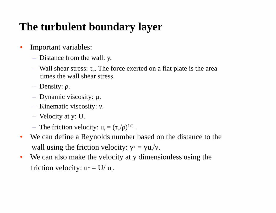
Obtaining accurate solutions
• When very accurate (say 2%) drag, lift, or torque predictions are
required, the boundary layer and flow separation require accurate
modeling.
• The following practices will improve prediction accuracy:
– Use boundary layer meshes consisting of quads, hexes, or prisms.
Avoid using pyramid or tetrahedral cells immediately adjacent to the
wall.
– After converging the solution,use the surface integral
reporting option to check if y+
is in the right range, and if not
refine the grid using
adaption.
– For best predictions use the
two-layer zonal model and
completely resolve the flow in
the whole boundary layer.
tetrahedral
volume mesh
is generated
automatically
prism layer
efficiently
resolves
boundary layer
triangular surface
mesh on car body
is quick and easy
to create
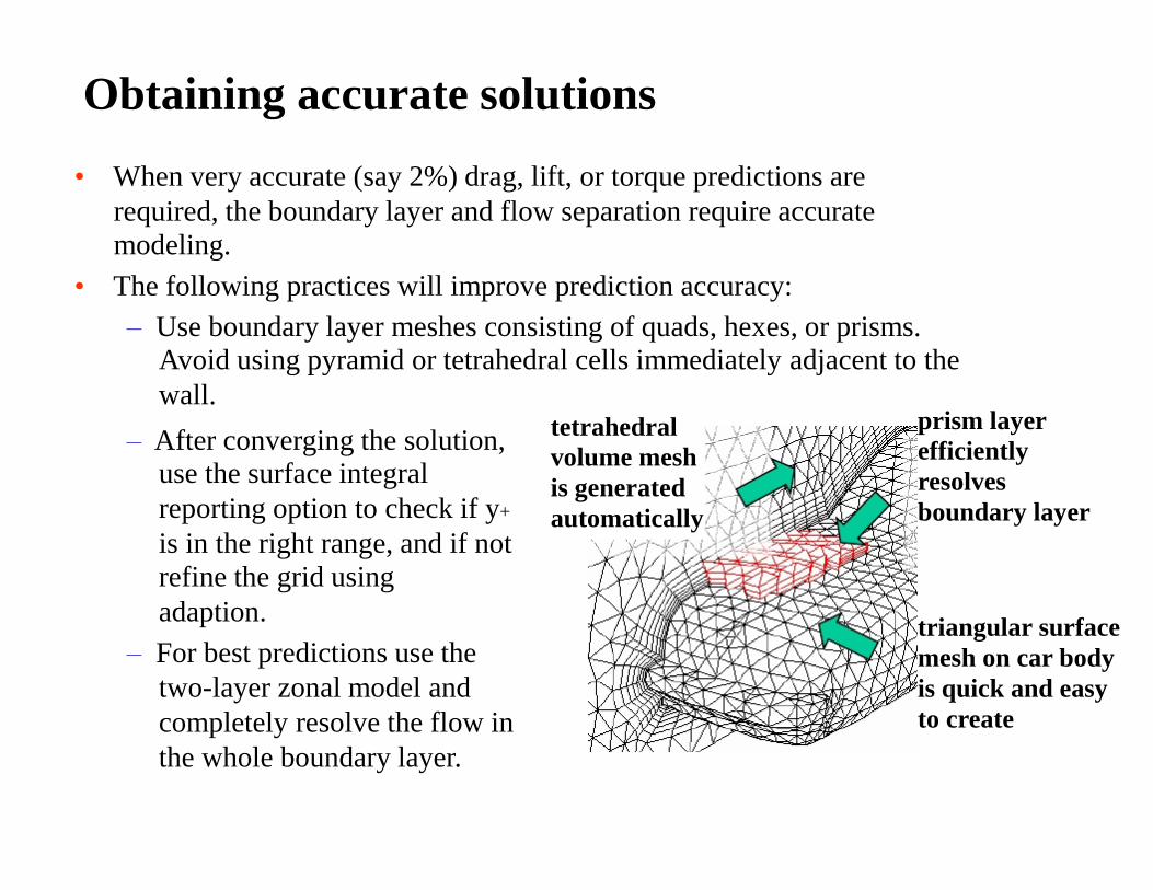
Summary
• Boundary layers require special treatment in the CFD model.
• The influence of pressure gradient on boundary layer attachment
showed that an adverse pressure gradient gives rise to flow
separation.
• For accurate drag, lift, and torque predictions, the boundary layer
and flow separation need to be modeled accurately.
• This requires the use of:
–
–
–
–
A suitable grid.
A suitable turbulence model.
Higher order discretization.
Deep convergence using the force to be predicted as a convergence
monitor.

Turbulence models

Turbulence models
• A turbulence model is a computational procedure to close thesystem of mean flow equations.
• For most engineering applications it is unnecessary to resolve the
details of the turbulent fluctuations.
• Turbulence models allow the calculation of the mean flow withoutfirst calculating the full time-dependent flow field.
• We only need to know how turbulence affected the mean flow.
• In particular we need expressions for the Reynolds stresses.
• For a turbulence model to be useful it:
–
–
–
–
must have wide applicability,
be accurate,
simple,
and economical to run.

Common turbulence models
• Classical models. Based on Reynolds Averaged Navier-Stokes(RANS) equations (time averaged):
– 1. Zero equation model: mixing length model.
– 2. One equation model: Spalart-Almaras.
– 3. Two equation models: k-ε style models (standard, RNG,realizable), k-ω model, and ASM.
– 4. Seven equation model: Reynolds stress model.
• The number of equations denotes the number of additional PDEsthat are being solved.
• Large eddy simulation. Based on space-filtered equations. Timedependent calculations are performed. Large eddies are explicitlycalculated. For small eddies, their effect on the flow pattern istaken into account with a “subgrid model” of which many stylesare available.

Prediction Methods

Boussinesq hypothesis
• Many turbulence models are based upon the Boussinesq
hypothesis.
– It was experimentally observed that turbulence decays unless there
is shear in isothermal incompressible flows.
– Turbulence was found to increase as the mean rate of deformation
increases.
– Boussinesq proposed in 1877 that the Reynolds stresses could be
linked to the mean rate of deformation.
• Using the suffix notation where i, j, and k denote the x-, y-, and z-
directions respectively, viscous stresses are given by:
• Similarly, link Reynolds stresses to the mean rate of deformation:

Turbulent viscosity
• A new quantity appears: the turbulent viscosity µt.
• Its unit is the same as that of the molecular viscosity: Pa.s.
• It is also called the eddy viscosity.
• We can also define a kinematic turbulent viscosity: νt = µt/ρ. Itsunit is m2/s.
• The turbulent viscosity is not homogeneous, i.e. it varies in space.
• It is, however, assumed to be isotropic. It is the same in all
directions. This assumption is valid for many flows, but not for all
(e.g. flows with strong separation or swirl).

nearly constant with typical values between 0.7 and 1.
Turbulent Schmidt number
• The turbulent viscosity is used to close the momentum equations.
• We can use a similar assumption for the turbulent fluctuation
terms that appear in the scalar transport equations.
• For a scalar property φ(t) = Φ + ϕ’(t):
• Here Γt is the turbulent diffusivity.
• The turbulent diffusivity is calculated from the turbulent viscosity,
using a model constant called the turbulent Schmidt number
• Experiments have shown that the turbulent Schmidt number is

Predicting the turbulent viscosity
• The following models can be used to predict the turbulent viscosity:
–
–
–
–
–
–
Mixing length model.
Spalart-Allmaras model.
Standard k-ε model.
k-ε RNG model.
Realizable k-ε model.
k-ω model.
• We will discuss some of these models

has dimension 1/s):
we can derive Prandtl’s (1925) mixing length model:
• Algebraic expressions exist for the mixing length for simple 2-Dflows, such as pipe and channel flow.
Mixing length model
• On dimensional grounds one can express the kinematic turbulentviscosity as the product of a velocity scale and a length scale:
• If we then assume that the velocity scale is proportional to thelength scale and the gradients in the velocity (shear rate, which
Further reading

Mixing length model discussion
• Advantages:
– Easy to implement.
– Fast calculation times.
– Good predictions for simple flows where experimental correlations
for the mixing length exist.
• Disadvantages:
– Completely incapable of describing flows where the turbulent length
scale varies: anything with separation or circulation.
– Only calculates mean flow properties and turbulent shear stress.
• Use:
– Sometimes used for simple external aero flows.
– Pretty much completely ignored in commercial CFD programs today.
• Much better models are available.

Spalart-Allmaras one-equation model
• Solves a single conservation equation (PDE) for the turbulent
viscosity:
– This conservation equation contains convective and diffusive
transport terms, as well as expressions for the production and
dissipation of νt.
– Developed for use in unstructured codes in the aerospace industry.
• Economical and accurate for:
– Attached wall-bounded flows.
– Flows with mild separation and recirculation.
• Weak for:
– Massively separated flows.
– Free shear flows.
– Decaying turbulence.
• Because of its relatively narrow use we will not discuss this modelin detail.

• We now need equations for k and ε.
The k-ε model
• The k-ε model focuses on the mechanisms that affect the
turbulent kinetic energy (per unit mass) k.
• The instantaneous kinetic energy k(t) of a turbulent flow is the
sum of mean kinetic energy K and turbulent kinetic energy k:
• ε is the dissipation rate of k.
• If k and ε are known, we can model the turbulent viscosity as:

Mean flow kinetic energy K
• The equation for the mean kinetic energy is obtained my multiplying U, Vand W to the Reynolds equation and it is as follows:
• Here Eij is the mean rate of deformation tensor.
• This equation can be read as:
–
–
–
–
–
–
(I) the rate of change of K, plus
(II) transport of K by convection, equals
(III) transport of K by pressure, plus
(IV) transport of K by viscous stresses, plus
(V) transport of K by Reynolds stresses, minus
(VI) rate of dissipation of K, minus
– (VII) turbulence production.

Turbulent kinetic energy k
• The equation for the turbulent kinetic energy k is as follows:
• Here eij’ is fluctuating component of rate of deformation tensor.
• This equation can be read as:
–
–
–
–
–
–
(I) the rate of change of k, plus
(II) transport of k by convection, equals
(III) transport of k by pressure, plus
(IV) transport of k by viscous stresses, plus
(V) transport of k by Reynolds stresses, minus
(VI) rate of dissipation of k, plus
– (VII) turbulence production.

Model equation for k
• The equation for k contains additional turbulent fluctuation terms,
that are unknown. Again using the Boussinesq assumption, these
fluctuation terms can be linked to the mean flow.
• The following (simplified) model equation for k is commonly used.
• The Prandtl number σk connects the diffusivity of k to the eddyviscosity. Typically a value of 1.0 is used.
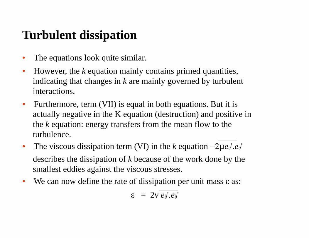
Turbulent dissipation
• The equations look quite similar.
• However, the k equation mainly contains primed quantities,
indicating that changes in k are mainly governed by turbulent
interactions.
• Furthermore, term (VII) is equal in both equations. But it is
actually negative in the K equation (destruction) and positive in
the k equation: energy transfers from the mean flow to the
turbulence.
describes the dissipation of k because of the work done by the
smallest eddies against the viscous stresses.
• We can now define the rate of dissipation per unit mass ε as:
• The viscous dissipation term (VI) in the k equation −2µeij'.eij'
ε = 2ν eij'.eij'

• The Prandtl number σε connects the diffusivity of ε to the eddyviscosity. Typically a value of 1.30 is used.
• Typically values for the model constants C1ε and C2ε of 1.44 and1.92 are used.
Model equation for ε
• A model equation for ε is derived by multiplying the k equation by
(ε/k) and introducing model constants.
• The following (simplified) model equation for ε is commonly used.
k-ε model discussion
• Advantages:
– Relatively simple to implement.
– Leads to stable calculations that converge relatively easily.
– Reasonable predictions for many flows.
• Disadvantages:
– Poor predictions for:
•
•
•
•
•
swirling and rotating flows,
flows with strong separation,
axisymmetric jets,
certain unconfined flows, and
fully developed flows in non-circular ducts.
– Valid only for fully turbulent flows.
– Simplistic ε equation.

More two-equation models
• The k-ε model was developed in the early 1970s. Its strengths as
well as its shortcomings are well documented.
• Many attempts have been made to develop two-equation models
that improve on the standard k-ε model.
• We will discuss some here:
–
–
–
–
–
k-ε RNG model.
k-ε realizable model.
k-ω model.
Algebraic stress model.
Non-linear models.

Improvement: RNG k- ε
• k-ε equations are derived from the application of a rigorous
statistical technique (Renormalization Group Method) to the
instantaneous Navier-Stokes equations.
• Similar in form to the standard k-ε equations but includes:
– Additional term in ε equation for interaction between turbulence
dissipation and mean shear.
– The effect of swirl on turbulence.
– Analytical formula for turbulent Prandtl number.
– Differential formula for effective viscosity.
• Improved predictions for:
– High streamline curvature and strain rate.
– Transitional flows.
– Wall heat and mass transfer.
• But still does not predict the spreading of a round jet correctly.
Improvement: realizable k-ε
• Shares the same turbulent kinetic energy equation as the
standard k-ε model.
• Improved equation for ε.
• Variable Cµ instead of constant.
• Improved performance for flows involving:
– Planar and round jets (predicts round jet spreading correctly).
– Boundary layers under strong adverse pressure gradients or
separation.
– Rotation, recirculation.
– Strong streamline curvature.
• The realizable k-ε model is a relatively recent development and differs from the standard k-epsilon model in two important ways:
• The realizable k-ε model contains a new formulation for the turbulent viscosity.• A new transport equation for the dissipation rate, ε, has been derived from an exact equation for the transport of the
mean-square vorticity fluctuation.
• The term "realizable'' means that the model satisfies certain mathematical constraints on the Reynolds stresses, consistent with the physics of turbulent flows. Neither the standard k-ε model nor the RNG k-ε model is realizable.

k-ω model
• This is another two equation model. In this model ω is an inverse
time scale that is associated with the turbulence.
• This model solves two additional PDEs:
– A modified version of the k equation used in the k-ε model.
– A transport equation for ω.
• The turbulent viscosity is then calculated as follows:
• Its numerical behavior is similar to that of the k-ε models.
• It suffers from some of the same drawbacks, such as the
assumption that µt is isotropic.
k
ωµt = ρ

38
Algebraic stress model
• The same k and ε equations are solved as with the standard k-ε
model.
• However, the Boussinesq assumption is not used.
• The full Reynolds stress equations are first derived, and then
some simplifying assumptions are made that allow the derivation
of algebraic equations for the Reynolds stresses.
• Thus fewer PDEs have to be solved than with the full RSM and it
is much easier to implement.
• The algebraic equations themselves are not very stable, however,
and computer time is significantly more than with the standard k-ε
model.
• This model was used in the 1980s and early 1990s. Research
continues but this model is rarely used in industry anymore now
that most commercial CFD codes have full RSM implementationsavailable.

Reynolds stress model
• RSM closes the Reynolds-Averaged Navier-Stokes equations by
solving additional transport equations for the six independent
Reynolds stresses.
– Transport equations derived by Reynolds averaging the product of
the momentum equations with a fluctuating property.
– Closure also requires one equation for turbulent dissipation.
– Isotropic eddy viscosity assumption is avoided.
• Resulting equations contain terms that need to be modeled.
• RSM is good for accurately predicting complex flows.
– Accounts for streamline curvature, swirl, rotation and high strain
rates.
• Cyclone flows, swirling combustor flows.
• Rotating flow passages, secondary flows.
• Flows involving separation.

< 10• For external flows: 1 < µ t /µ
Setting boundary conditions
• Characterize turbulence at inlets and outlets (potential backflow).
– k-ε models require k and ε.
– Reynolds stress model requires Rij and ε.
• Other options:
– Turbulence intensity and length scale.
• Length scale is related to size of large eddies that contain most of
energy.
• For boundary layer flows, 0.4 times boundary layer thickness: l ≈ 0.4δ99.
• For flows downstream of grids /perforated plates: l ≈ opening size.
– Turbulence intensity and hydraulic diameter.
• Ideally suited for duct and pipe flows.
– Turbulence intensity and turbulent viscosity ratio.

Comparison of RANS turbulence models
Recommendation
• Start calculations by performing 100 iterations or so with standard k-ε
model and first order upwind differencing. For very simple flows (no swirl
or separation) converge with second order upwind and k-ε model.
• If the flow involves jets, separation, or moderate swirl, converge solution
with the realizable k-ε model and second order differencing.
• If the flow is dominated by swirl (e.g. a cyclone or unbaffled stirred
vessel) converge solution deeply using RSM and a second order
differencing scheme. If the solution will not converge, use first order
differencing instead.
• Ignore the existence of mixing length models and the algebraic stress
model.
• Only use the other models if you know from other sources that somehow
these are especially suitable for your particular problem (e.g. Spalart-
Allmaras for certain external flows, k-ε RNG for certain transitional flows,
or k-ω).

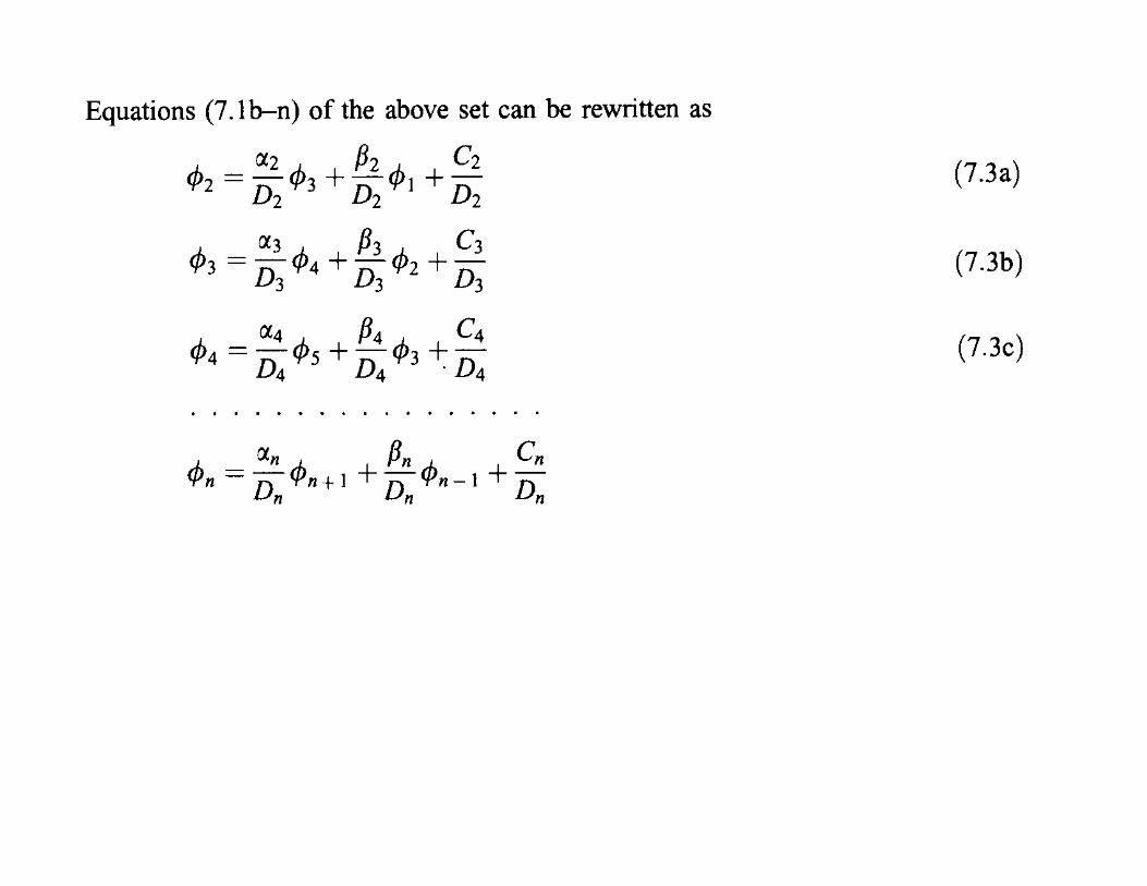
Tri-diagonal matrix algorithm(TDMA)

Consider a system of equations that has a tri-diagonal form
In the above set of equations 1 and n+1 are known boundary values. The general
form of any single equation is


End