
Turbulence Modelling for Internal Cooling of Gas-Turbine ...lada/postscript_files/jonas_PhD.pdf ·...
141
T HESIS FOR THE DEGREE OF DOCTOR OF P HILOSOPHY Turbulence Modelling for Internal Cooling of Gas-Turbine Blades J ONAS B REDBERG Department of Thermo and Fluid Dynamics C HALMERS UNIVERSITY OF T ECHNOLOGY G ¨ OTEBORG,S WEDEN, 2002
Transcript of Turbulence Modelling for Internal Cooling of Gas-Turbine ...lada/postscript_files/jonas_PhD.pdf ·...

THESIS FOR THE DEGREE OF DOCTOR OF PHILOSOPHY
Turbulence Modelling forInternal Cooling ofGas-Turbine Blades
JONAS BREDBERG
Department of Thermo and Fluid DynamicsCHALMERS UNIVERSITY OF TECHNOLOGY
GOTEBORG, SWEDEN, 2002

Turbulence Modelling for Internal Cooling of Gas-Turbine BladesJONAS BREDBERGISBN 91-7291-181-66
c�
JONAS BREDBERG, 2002
Doktorsavhandlingar vid Chalmers tekniska hogskolaNy serie nr 1863ISSN 0346-718X
Institutionen for termo- och fluiddynamikChalmers tekniska hogskolaSE-412 96 Goteborg, SwedenPhone +46-(0)31-7721400Fax: +46-(0)31-180976
Printed at Chalmers reproserviceGoteborg, Sweden 2002

Turbulence Modelling forInternal Cooling of Gas-Turbine Blades
by
JONAS BREDBERG
Department of Thermo and Fluid DynamicsChalmers University of TechnologySE-412 96 GOTEBORG, SWEDEN
Abstract
Numerical simulations of geometrical configurations similar to thosepresent in the internal cooling ducts within gas turbine blades havebeen performed. The flow within these channels are characterized byheat transfer enhancing ribs, sharp bends, rotation and buoyancy ef-fects. On the basis of investigations on rib-roughened channel it isconcluded that the frequently employed two-equation turbulence mo-dels ( ����� , ����� ) cannot predict heat transfer in separated regionswith a correct Reynolds number dependency. Extensions to non-linearmodels, such as EARSM, do not alters this inaccurate tendency. Theimportance of the length-scale determining equation for this behaviouris discussed. A low-Reynolds number (LRN) ����� turbulence model,with improved heat transfer predictions, is proposed. The new modelincludes cross-diffusion terms which enhances free-shear flow predicta-bility. A new method to reduce the mesh sensitivity for LRN turbu-lence models is proposed. Within the concept of finite volume codes itis shown that through a carefully treatment of the integrations for thefirst interior control volume, minor modifications results in a signifi-cant reduced grid dependency for near-wall sensitive parameter. Thelatter modification in conjunction with the new ���� turbulence modelresults in an accurate and robust method for simulating large and com-plex geometries within the frame of internal cooling of turbine blades.
Keywords: gas turbine blades, U-bend, rib-roughened channel, rota-tion, heat transfer, cooling, turbulence model, EARSM, ���� , ����
iii


List of Publications
This thesis is based on the work contained in the following papers:
I. J. Bredberg and L. Davidson”Prediction of flow and heat transfer in a stationary two-dimensionalrib roughened passage using low-Re turbulent models”In Proceedings of 3:rd European Conference on Turbomachinery:Fluid Dynamics and Thermodynamics, pages 963-972, IMechE1999.
II. J. Bredberg, L. Davidson and H. Iacovides”Comparison of Near-wall Behavior and its Effect on Heat Trans-fer for ����� and ��� � Turbulence Models in Rib-roughened 2DChannels”In Proceedings of 3:rd Int. Symposium on Turbulence, Heat andMass Transfer, pages 381-388, eds. Y. Nagano and K. Hanjalicand T. Tsuji, Aichi Shuppan 2000.
III. J. Bredberg, S.-H. Peng and L. Davidson”On the Wall Boundary Condition for Computing Turbulent HeatTransfer with �� � Models”In Proceedings of the ASME Heat Transfer Division - 2000, HTD-Vol. 366-5, pages 243-250, ed. J.H. Kim, ASME 2000.
IV. J. Bredberg”On the Wall Boundary Condition for Turbulence Models”Report 00/4, Department of Thermo and Fluid Dynamics, Chal-mers University of Technology, 2000.
V. J. Bredberg”On Two-equation Eddy-Viscosity Models”Report 01/8, Department of Thermo and Fluid Dynamics, Chal-mers University of Technology, 2001.
v

VI. J. Bredberg, S.-H. Peng and L. Davidson”An improved ��� � turbulence model applied to recirculatingflows”Accepted for publication in Int. J. Heat and Fluid Flow, 2002.
VII. J. Bredberg and L. Davidson”Prediction of turbulent heat transfer in stationary and rotatingU-ducts with rib roughened walls”Accepted to 5:th International Symposium on Engineering Turbu-lence Modelling and Measurements, 2002.
VIII. J. Bredberg and L. Davidson”Low-Reynolds Number Turbulence Models: An Approach for Re-ducing Mesh Sensitivity”Submitted for journal publication.
Relevant scientific publications not included in this thesis:
9. J. Bredberg and L. Davidson”Case 7.2: Two-Dimensional Flow and Heat Transfer over a SmoothWall Roughened with Squared Ribs”In Proceedings of 7:th ERCOFTAC/IAHR Workshop on RefinedTurbulence Modelling, 1998.
10. J. Bredberg”Prediction of Flow and Heat Transfer in 3-D Rib Roughened Pas-sage using Low-Re Turbulent Models”In Proceedings of GTC annual meeting, 1998.
11. J. Bredberg”Prediction of Flow and Heat Transfer Inside Turbine Blades usingEARSM, � � � , and � � � Turbulence Models”Thesis for the Degree of Licentiate of Engineering, Report 99/3,Department of Thermo and Fluid Dynamics, Chalmers Universityof Technology, 1999.
12. J. Bredberg”TCP4, Turbine Blade Internal Cooling”In Proceedings of GTC annual meeting, 1999.
vi

13. J. Bredberg”TCP4, Numerical Investigation of Internal Cooling of TurbineBlades”In Proceedings of GTC annual meeting, 2000.
14. J. Bredberg”TCP4, Turbine Blade Internal Cooling”In Proceedings of GTC annual meeting, 2001.
vii


Acknowledgments
This work was carried out at the Department of Thermo and FluidDynamics, Chalmers University of Technology, Gothenburg, Sweden.The work could not have been done without the help of many persons,of whom the following are specially acknowledged.
I would like to express my greatest precautions toward my supervi-sor Prof. L. Davidson, for all his advice, guidance and support to thistime. I hope it will continue.
This project, Turbine Blade Internal Cooling, is part of the groupTurbine Cooling Performance within GTC, a national Gas Turbine Cen-ter, headed by Sven-Gunnar Sundkvist. GTC is supervised and fundedby Statens Energimyndigheten and sponsored by Volvo Aero Corpora-tion and Alstom Power. The financial and scientific support by all partsis gratefully acknowledged.
I would also like to thank Dr. S-H. Peng, at FOI, which has beena great inspiration and given valuable comments, especially regardingthe work with turbulence models. The latter work would have beenseverely deprived without the influence from you.
Furthermore I would like to thank Dr. H. Iacovides, at UMIST, for avery fruitful visit in Manchester, UK, in 1998. You gave most importantcomments and suggestions for the work in Paper II. The help of Dr.T. Craft for this work and useful discussions with Dr. M. Raisee isalso acknowledged. The supply of experimental data from UMIST fora number of the simulations performed are greatly appreciated.
ix


Contents
Abstract iii
List of Publications iv
Acknowledgments viii
1 Introduction 11.1 The Gas Turbine . . . . . . . . . . . . . . . . . . . . . . . . 11.2 Increasing Efficiency through Cooling . . . . . . . . . . . 21.3 Flow Phenomena Inside Turbine Blades . . . . . . . . . . 5
2 Fluid Motion and Heat Transfer 92.1 Governing Equations . . . . . . . . . . . . . . . . . . . . . 9
2.1.1 Continuity . . . . . . . . . . . . . . . . . . . . . . . 92.1.2 Momentum . . . . . . . . . . . . . . . . . . . . . . . 102.1.3 Energy . . . . . . . . . . . . . . . . . . . . . . . . . 102.1.4 Rotational Modifications . . . . . . . . . . . . . . . 10
2.2 Flow Models . . . . . . . . . . . . . . . . . . . . . . . . . . 112.2.1 DNS/LES . . . . . . . . . . . . . . . . . . . . . . . . 112.2.2 RANS . . . . . . . . . . . . . . . . . . . . . . . . . . 122.2.3 Other flow models . . . . . . . . . . . . . . . . . . . 13
2.3 Turbulence Models with Special Reference to Rotation . 142.3.1 Reynolds stress models . . . . . . . . . . . . . . . . 142.3.2 Eddy-viscosity models . . . . . . . . . . . . . . . . 172.3.3 EARSM and non-linear EVMs . . . . . . . . . . . . 19
2.4 Turbulent Heat Transfer Models . . . . . . . . . . . . . . 19
3 Flow phenomena in turbine blades 213.1 Walls . . . . . . . . . . . . . . . . . . . . . . . . . . . . . . 213.2 Ribs – blockage . . . . . . . . . . . . . . . . . . . . . . . . 223.3 Secondary flows . . . . . . . . . . . . . . . . . . . . . . . . 31
xi

3.4 Bends – curvature . . . . . . . . . . . . . . . . . . . . . . . 343.5 Rotation . . . . . . . . . . . . . . . . . . . . . . . . . . . . 363.6 Review, experiments and numerical simulations with re-
ference to turbine blade internal cooling. . . . . . . . . . . 393.6.1 Experiments: . . . . . . . . . . . . . . . . . . . . . . 403.6.2 Numerical simulations: . . . . . . . . . . . . . . . . 41
4 Numerical Considerations 494.1 Numerical Method . . . . . . . . . . . . . . . . . . . . . . 494.2 Discretizing Schemes and Mesh Dependency . . . . . . . 504.3 Boundary Conditions . . . . . . . . . . . . . . . . . . . . . 554.4 Periodic Flows . . . . . . . . . . . . . . . . . . . . . . . . . 564.5 2D Approximations . . . . . . . . . . . . . . . . . . . . . . 58
5 Results and Discussion 615.1 2D Rotating Channel . . . . . . . . . . . . . . . . . . . . . 615.2 3D rib-roughened channel with periodic boundary condi-
tions . . . . . . . . . . . . . . . . . . . . . . . . . . . . . . . 675.2.1 Stationary: . . . . . . . . . . . . . . . . . . . . . . . 695.2.2 Rotating: . . . . . . . . . . . . . . . . . . . . . . . . 73
6 Summary of Papers 816.1 Paper I . . . . . . . . . . . . . . . . . . . . . . . . . . . . . 816.2 Paper II . . . . . . . . . . . . . . . . . . . . . . . . . . . . . 826.3 Paper III . . . . . . . . . . . . . . . . . . . . . . . . . . . . 836.4 Paper IV . . . . . . . . . . . . . . . . . . . . . . . . . . . . 856.5 Paper V . . . . . . . . . . . . . . . . . . . . . . . . . . . . . 856.6 Paper VI . . . . . . . . . . . . . . . . . . . . . . . . . . . . 866.7 Paper VII . . . . . . . . . . . . . . . . . . . . . . . . . . . . 886.8 Paper VIII . . . . . . . . . . . . . . . . . . . . . . . . . . . 88
7 Conclusions 91
Bibliography 91
xii

Chapter 1
Introduction
A general introduction to the gas turbine engine is given.The importance of higher gas temperatures and the meansof achieving this is discussed. A schematic cooling schemefor turbine blades is shown. The physical phenomenas dueto geometrical constraints and applied forces are addressed.
1.1 The Gas TurbineOf the various means of producing either thrust or power, the gas-turbine engine is one of the most satisfactory. Its main advantages are:exceptional reliability, high thrust-to-weight ratio, and relative free-dom of vibration. The work from a gas-turbine engine may be giveneither as torque in a shaft or as thrust in a jet. A gas-turbine consist ofthe following main parts: an inlet, a compressor, a combustor, a turbineand an exhaust, Fig. 1.1.
The inlet section may involve filters, valves and other arrangements
Figure 1.1: RM12, Gas Turbine
1

Jonas Bredberg, Internal Cooling of Gas-Turbine Blades
to ensure a high quality of the flow. In flying applications it is of impor-tance to pay special consideration to the inlet as the ram-effect couldboost the thrust significantly.
The pressure of the air is increased in the compressor, which is di-vided into several stages. There are two main types of compressors,radial – where the air enters axial but exits radially, or the more com-mon axial compressor – where the flow is primarily axial. The rotationof the compressor increases the velocity of the air with the following dif-fusers converts the dynamic pressure (velocity) to static pressure. Thecompressor is connected to the turbine via a shaft running through thecenter of the engine.
The operation of a gas-turbine relies on that the power gained fromthe turbine exceeds the power absorbed by the compressor. This isensured by the addition of energy in the combustor, through ignitingfuel in special purposed burners. The design and operation of theseburners are vital for a high efficient engine if low emissions are to beachieved.
The highly energetic gas from the combustor is expanded through aturbine, which drives the compressor in the front of the engine. Afterthe turbine the gas still contains a significant amount of energy whichcan be extracted in various forms. In aircrafts the surplus energy istransformed into a high velocity jet in the nozzle which is the drivingforce that propels the vehicle through the air. The jet velocity andhence thrust could be further increased, through re-heating the gasin an afterburner. This is common in high performance aircraft, espe-cially for military applications. For stationary, power generating gas-turbines, the extra energy is converted into shaft-power in a power-turbine.
1.2 Increasing Efficiency through Cooling
Through the increased environmental awareness and higher fuel costs,there have lately been a strong strive towards enhanced efficiencies forall automotive propulsions. For gas turbines applications, especially inaircraft, not only the specific fuel consumption (SFC) is of importancebut also the specific work output. The former is equivalent to the in-verse of the efficiency while the latter is a measure of the compactnessof the power plant, ie. the effectiveness. The maximum theoretical
2

Chap. 1: Introduction
Figure 1.2: Turbine Entry Temperature (Copyright Rolls Royce plc)
efficiency of a gas turbine cycle is given by the Carnot efficiency as:
����� ������ (1.1)
where��
is the inlet temperature and���
the turbine entry temperature(TET). Increasing
���yield a direct improvement in the efficiency, � .
The performance of practical cycles are however lower, due to pressureand massflow losses, friction, components efficiency, non-ideal fluidsetc. When these losses are taken into account, the efficiency of thesimple gas turbine cycle1 becomes dependent not only of the tempera-ture ratio, as in the Carnot process, but also the compressor pressureratio. Thus the gas turbine industry are trying to reach both higherturbine temperatures as well as increased pressure ratio, to improvethe efficiency and effectiveness of tomorrows engines.
1The simple cycle consists of a compressor, a combustor and a turbine.
3

Jonas Bredberg, Internal Cooling of Gas-Turbine Blades
Figure 1.3: Cooling schemes, Inlet Guide Vane (Copyright Rolls-Royceplc)
Even though exotic materials are used for the most stressed envi-ronments, these have for the last decades been unable to withstandthe demanded TET without yielding to the harsh environment. High-strength material such as nickel and cobalt based super alloys, (eg.Inco 738 and Rene 220) will all weaken from increased temperatu-res, and since the loads in a rotating turbine are extremely high, thestructure fails if not counter-measures are taken. The introductionof relatively cool gas from the compressor in well selected places inthe turbine extends the engine endurance, and was in practise alreadyduring the second world war. Figure 1.2 shows the increases in TETthrough the introduction of different cooling techniques.
The highest temperatures loads are found at the exit of the com-bustor, and in the first turbine stage. A comprehensive cooling systemare thus needed for the inlet guide vanes (IGV). A conceptional viewof such as system is shown in Fig. 1.3. These vanes employs bothexternal cooling (film cooling), and internal cooling (convection- andimpingement-cooling). The vanes are perforated by a number of smallholes, through which compressed air is ejected. If correctly designedthese holes will supply a cool protective air-film covering the vanes.
4

Chap. 1: Introduction
This technique is called film cooling. The same type of cooling is ap-plied to the platforms, along the tip (shroud) and root (hub) of the vane.Internally the vanes are cooled using convection and impingement te-chniques. The compressed air is guided through ducts which cools thevane-material by means of convection/conduction from the inside. Thisapproach is however not as effective, as the film-cooling technique, andhence a number of measures are generally made to increase the heattransfer. Ribs, positioned orthogonally to the flow, are introduced in theducts, which makes the flow repeatedly separate and re-attach with anincrease in turbulence level and a consequently enhancement of theheat transfer. These rib-roughened ducts are designed in a serpentinefashion and can completely fill out the inside of a vane. Finally the coo-ling air can be guided vertically towards some specifically hot regionsfor effective cooling. The latter is called impingement cooling.
It should be noted that the available pressure-difference betweenthe internal cooling air and the external main gasflow, is severely li-mited. Hence there is a restriction to the number of turns, ribs andother pressure reducing features that can be employed within a givenpassage. There is also a construction limit to how complex the inte-rior could be made, while still maintaining productivity and being cost-effective. Contemporary gas turbines may use as much 15% of the totalmassflow for cooling air. Even though there is significant advantageof increasing TET, the use of cooling air for achieving this has somedrawbacks: 1) the addition of cool air into the main stream reduces thework output from the turbines; 2) protective films along the vanes com-plicates the aero-thermal design of the blades, as the momentum andblockage effect introduced by the cooling air changes gas angles depen-dent on engine loads; 3) cooling air does not participate in the energyenriching process in the combustor and hence the effective massflow isreduced.
1.3 Flow Phenomena Inside Turbine Bla-des
The turbine in a gas turbine engine consists of several stages, eachstage having both a stationary and a rotating set of blades. The sta-tionary row is positioned upstream the rotating row, to guide the flowfrom an axial to a tangential-axial direction in order to drive the tur-bine. To distinguish between the two rows one has chosen to denote the
5

Jonas Bredberg, Internal Cooling of Gas-Turbine Blades
PSfrag replacements
Coriolis
Inlet
Outlet
Heatflux
�
Figure 1.4: The interior of a turbine blade
stationary aerofoils as vanes and the rotating counter-parts are refer-red to as blades. The turbine blades, similar to turbine vanes need to becooled using pressurized air from the compressor. The lower externalgas temperature however reduces the necessary complexity of the coo-ling system as well as the amount of air needed, compared to the IGVdiscussed above, Fig. 1.3. The blades are however stressed by the rota-tional forces, (ie. the Coriolis- and the centrifugal-forces), in addition tothe temperature loads. These rotational induced forces complicates theflow structure within the ducts, making the design and construction ofturbine blades one of the most challenging and expansive industrialenterprise today. Figure 1.4 shows a schematic view of a U-bend sec-tion, located in the center of the turbine blades. In the figure several ofthe flow-field modifications as a result of imposed conditions, both geo-metrical and force related are presented. The matrix below connects
6

Chap. 1: Introduction
the resulting flow phenomena due to the enforced physical conditions.
Shea
ring
Sec.
flow
Sepa
ratio
nAc
c-D
ecSt
abili
zing
Buoy
ancy
Bends X X X XCorners XHeating X XRibs X X X XRotation X X XWalls X
Note that only the main and direct effects are listed. Heating eg. mayunder certain condition result in such destabilizing condition that theflow separates. In the table it is inferred that stabilizing also refers tothe opposite destabilizing condition. The consequence and the difficul-ties the listed effects impose on numerical simulations are discussed inChapter 3.
7

Jonas Bredberg, Internal Cooling of Gas-Turbine Blades
8

Chapter 2
Fluid Motion and HeatTransfer
The equations governing fluid motion, the Navier-Stokes equa-tions are displayed. An overview of turbulence and heattransfer models with literature references are given. Spe-cial references to modification due to rotational induced tur-bulence are made.
2.1 Governing EquationsThe equations that govern fluid motion and heat transfer are the con-tinuity, momentum and energy equations. These equations, were in-dependently constructed by Navier (1827) and Stokes (1845) and arereferred to as the Navier-Stokes equations. These can be formulatedin either a conservative form, or in the non-conservative form. For anearly incompressible fluid, the density is constant, and consequentlymany text-books gives the Navier-Stokes equations on a density nor-malized formulation.
2.1.1 ContinuityThe continuity equation states the conservation of mass, which for allbut nuclear-reaction environments is valid. The conservative form is:
��������
��������� �� (2.1)
9

Jonas Bredberg, Internal Cooling of Gas-Turbine Blades
2.1.2 MomentumThe momentum equation describes a force-balance, which – from theNewtons second law – states that the mass times the acceleration isequal to imposed forces. The forces are divided into body force � ,eg. the gravitational force, and surface forces,
� ��. The surfaces for-
ces are normally written as a combination of pressure (normal stress)and viscous stresses (shear) as:
� �� � ����� �� �� �� (2.2)
Assuming a Newtonian incompressible fluid the momentum equationsbecomes:
���� ��� �
����� ������� � � � � � � ���
���� ��������������� ���� (2.3)
where � is any additional body-forces that can effect the fluid motionsuch as rotation, a magnetic- or electric-field etc.
2.1.3 EnergyThe first law of thermodynamics states that the exchange of energy fora system is the result of applied work and heat transfer through thatregion. In its most complete formulation the energy equations is givenas [154]:
���������� �
������������� � ��� � � ���
���� ������� � �� � �� � (2.4)
where� ��
is the surface forces similar to the viscous and pressure termsin the momentum equations.
�!�is the total internal energy, including
the kinetic energy. The energy equation as displayed above is howeverseldom used and instead the simplified temperature equation is ap-plied:
����"$# ���� �
����"$# �� ����� �
�����
% � "$#�'& � �����)( (2.5)
2.1.4 Rotational ModificationsThe Navier-Stokes equations are derived and valid for a Newtonian in-ertial coordinate system, ie. system without any forced acceleration. A
10
Chap. 2: Fluid Motion and Heat Transfer
coordinate system fixed in a rotating structure however involves bothCoriolis and centripetal accelerations and hence the commonly appliedequations are invalid. It is however straight forward to derive rotatio-nal modified NS-equations, see [19].
Assuming that the coordinate system has a fixed1 location of originand that the rotation velocity is constant, ie. neglecting any additionalacceleration terms due to angular acceleration, the extra terms (on theLHS) in the momentum equation are:
����� � �����
���� � � � � ��
(2.6)���� � � �
���� � � ���(2.7)
These terms are often considered as a body-force modification to theNavier-Stokes equation and hence included, with a change in sign, onthe RHS. There is no rotational modification to either the continuity ortemperature/energy equation.
2.2 Flow ModelsThe Navier-Stokes equations are composed of non-linear partial dif-ferential equations with an intricate complex dependency within theequation system. Partial differential equations are apart from somespecific cases, not solvable using known mathematical tools hence theNS-equations impose a severe obstacle to the physical world. There areonly a very small number of flows that entitle one to simplify the gover-ning equations in such a way that it is possible to achieve an analyticalsolution. Consequently for most cases, one is referred to numericallysolve the Navier-Stokes equations. The highest level of fidelity is givenby Direct Numerical Simulations (DNS’s) and Large Eddy Simulations(LES’s). Numerical simulations performed using Reynolds AveragedNavier Stokes (RANS) solvers are apart from numerical approxima-tions also affected by physical approximations – in the models for theturbulence field.
2.2.1 DNS/LESDirect Numerical Simulations (DNS’s) and Large Eddy Simulations(LES’s) both solve the equations in the four-dimensional room, time
1The coordinate could also translate at a constant velocity, akin to Newtons secondlaw of motion
11

Jonas Bredberg, Internal Cooling of Gas-Turbine Blades
and space. The additional modelling in LES as compared to DNS isthe introduction a sub-grid scale (SGS) model [184], which legitimacyis based on the assumption of isotropocy of the smallest scales. For agiven cut-off wave-length, normally related to the grid-size, LES don’tresolve the smallest length-scales but rather approximate them usingthe SGS-model. DNS’s are very appreciated as they are consideredequally, or even more accurate than experiments. The numerical modelenable unphysical although theoretical interesting flows to be simula-ted, with a degree of control unachievable in a laboratory. The numeri-cal accuracy in DNS’s are usually much higher than the uncertainty inany measuring tool. A major drawback is however that the simulationsare computational expansive and can only be performed for a limitednumber of flows, all with relatively low Reynolds numbers.
2.2.2 RANSNearly all numerical simulations are performed using various RANS-models, as a consequence of the excessive computational resources nee-ded for a DNS. Reynolds [173] proposed that the quantities in the NS-equation could be divided into a mean and a fluctuating part:
� � � � ���(2.8)
where the mean part is the time-average of a parameter over a certaintime. The averaging time needs to be longer than the small turbulentfluctuation, however shorter than any mean flow oscillating period,such as pumping frequencies, or rotation-frequency induced fluctua-tions. If Reynolds decomposition is applied to the Navier-Stokes equa-tion the result is an equivalent set of equations, the Reynolds AveragedNavier-Stokes equations2. The difference between these and the origi-nal are that the RANS equations only involves time-averaged quan-tities. The time averaging procedure however produces an additionalterm, the Reynolds stresses:� �� � � � � �� (2.9)
which are unknown and need to be modelled using a turbulence model.This is referred to as the closure problem with Reynolds averaging.
There are two distinct approaches to model the Reynolds stresses,either the eddy-viscosity models (EVM), or the Reynolds stress models
2See the comprehensive analysis and alternative approaches (eg. Favre-averaging) in Hinze [75].
12

Chap. 2: Fluid Motion and Heat Transfer
(RSM). In the latter the actual stresses are solved, while in the for-mer the Boussinesq [17] hypothesis is employed to estimate � �� , seeEq. 2.18. In its simplest form, the eddy-viscosity, ��� is computed basedon some geometrical/flow conditions. In the commonly employed two-equation turbulence models, the eddy-viscosity is computed using twoturbulent quantities, the turbulent kinetic energy, � � ���� � � � � � � anda length-scale determining quantity. In a strive to enhance the perfor-mance of the two-equation EVMs researchers have proposed non-linearEVMs, which include, apart from the Boussinesq hypothesis, additio-nal terms to determine the eddy-viscosity.
The ASM and EARSM (or EASM) are a different case, they com-pute the Reynolds stresses using algebraic equations. In ASM the con-vective and diffusion terms in the Reynolds stress transport equationsare approximated using anisotropized versions (through multiplicationwith � � � ���� � ) of the same terms in the turbulent kinetic energy. TheASM thus only need to solve two transport equations, that for � and anadditional secondary turbulence quantity. The Reynolds stresses couldthen be estimated using the constructed algebraic relations. This mo-delling approach is however prone to numerical instable solution andare seldom used.
It is possible, through the use of the Cayley-Hamilton theorem to de-rive the complete tensorial relation for the Reynolds stresses, expres-sion in the strain-rate tensor, � �� and the rotation tensor,
� ��. The com-
plete set involves ten terms with their respectively coefficients [164].Using these expressions the Reynolds stresses can, in a second momentclosure sense, be exactly computed. EARSMs are thus theoreticallymore correct than non-linear EVMs, although the final expressions areoften confusingly similar. They differ in the approach used for the coef-ficients in the tensor groups, which in EARSMs, at least for 2D-flows,can be based on derived analytic expressions [203].
2.2.3 Other flow modelsThe above discussed RANS-models are all single-point correlations clo-sures, ie. the turbulence quantities are evaluated at a single point inspace and time. The consequence of this is that these models cannot re-alize the multitude of length-scales occurring in a turbulent flow, cont-rary to DNS and LES. Furthermore RANS models are unable to dis-tinguish the physical processes governing the far-field turbulent inte-ractions to those associated with the nearly isotropic local turbulence.It is well known that these processes are distinctly different and it is
13

Jonas Bredberg, Internal Cooling of Gas-Turbine Blades
important to faithfully capture both. Mathematical models which onlycontains a single length-scale (or time-scale) can neither incorporatethese different physical process nor model the important energy trans-fer from low to high wave-number. Single-point turbulence model canthus never be a general method to predict turbulent flowfields [56].
Models which incorporate several length-scales, either properly fromthe two-point correlation, � �� , or from simplified assumptions, shouldbe able to improve predictions in complex flows. Hanjalic et al. [72]devised a two-scale model based on the ��� � concept which involvesfour transport equations instead of two. Guo and Rhode refined themodel and proposed a two-scale [108] and a three-scale [61] � � � modelboth yielding a substantial improvements compared to the standard� ��� model3.
A special reference is here made to the structured based models byReynolds et al. [174] and the TSDIA (Two-Scale Direction InteractionAnalysis) based model by Yoshizawaw [213], which both are able toinclude rotational induced turbulence in a natural way.
2.3 Turbulence Models with Special Refe-rence to Rotation
2.3.1 Reynolds stress modelsReynolds Stress Models (RSM) ([69],[118], [185]), solves the Reynoldsstresses, � �� � � � � �� , using individual transport equations. RSM ba-sed RANS-codes thus include, apart from three momentum equation,six stress equation, and an additionally length-scale determining equa-tion. The transport equations for the Reynolds stresses are, with mo-dification made for rotational induced production:
� � ��� � � � �� ��� �� ��� �� ��� �� � � �������� � �
� ������� � (2.10)
where����
is the shear production term, � �� the rotational productionterm, � �� the pressure-strain term, �
��the dissipation term,
���� tur-bulent transport (diffusion) term, and
����� the viscous diffusion term.
3The three-scale model however gives only a marginal improvement compared tothe two-scale model.
14
Chap. 2: Fluid Motion and Heat Transfer
These are, see [19]:���� � � %� � � � �
� ����� � � � �� � � � � � ��� � (
� �� � � � � ������� � � � � � � � �
��� � �� � � ���� �� � � �� % � � �
����� � � � ������ (
��� � � � � � ���� �
� � ����� �
� ��� � � �� � � �� � ��� � � �� � �� � � � � � � � � � ����
� ��� � � � � � � � ����� �
The production terms, and the viscous diffusion term are exact, whilethe other terms need to be modelled.
The exact formulation of the production terms is a fundamentallyadvantage of the RSMs compared to the EVMs. For a 2D dimensionalshear-flow (streamwise in
�-direction) undergoing orthogonally rota-
tion with� � ���
the non-zero production terms are:
i=1,j=1 i=2,j=2 i=1,j=2����� � � � �� � � � � 0 � ���� � � � �
� �� � � � � � �� � � � � � � � � � � � � � � �
The � -equation ( � � ���� � � � � � � ) in two-equation EVM is unaffected byrotation as � � � � � ��� �� . In addition the shear-stress, � �� � , is inaccura-tely estimated through the neglection of the rotational production ( � � � )via the isotropic estimation of the normal stresses, ie. � � � � � � :� � � � � ��� � �� � � � ��� � ��� � ����� (2.11)
This state of affairs necessitates that two-equation EVMs need to in-clude ad hoc modifications in order to predict rotational induced turbu-lence. Although RSMs predict the correct level of production, the mo-delling of the other terms in the Reynolds stress equations normallyexclude any influence by rotation, even though it is well known thatsuch dependency exists, see [19].
15

Jonas Bredberg, Internal Cooling of Gas-Turbine Blades
Following Kolmogorov the dissipation rate is assumed to be isotro-pic: �
�� � � ��� � � �� and modelled using its own scalar transport equation[70]:
� �� � � � "�� � � � � � � �� � ����� � � "�� � � ���
���� �
% "�� ��� � � � � �
����� � ( (2.12)
where"�� ��� "�� � and
"��are tunable constants. This model becomes iden-
tical to the � -equation used in the � � � model by Jones and Launder[101], when the Reynolds stresses ( � � � � � and � � � � � � ) are approximatedusing the Boussinesq hypothesis. Hanjalic and Launder [71] formula-ted a low-Reynolds number modification of Eq. 2.12 for use in RSMs,which includes modelling for anisotropic levels of the dissipation rate.It can be shown [19], that the dissipation rate is effected by the ro-tation, however these terms involve gradients of the velocity fluctua-tions and cannot be implemented exactly. A well established rotational-modification to the � -equation is to let the destruction term coefficient,"�� � , vary depending on the rotational ’Richardson number’, see Brad-shaw [18] (2D4):
��� � � � �% � �� � � � � ( �
% � �� � ( � � � � �� � � � � (2.13)
Launder et al. [119] proposed to replace � � � � � with the turbulent time-scale � � � � � , however in the context of the similar curvature effect.Models for length-scale correction have been proposed by eg. Bardinaet al. [10], Hellsten [74], Howard et al. [77] and Shimomura see [214].These models are either incorporated in the destruction term, , oradded as an extra source term,
�, in the � or � -equation:
� � � "�� � � � � "� ��� � � �� Howard et al.�� � � " � �
�Bardina et al.�� � � " � � �
���� � � � �� �� Shimomura
�� ��
� � "� ���
� � Hellsten
The pressure-strain term is divided into two parts, the slow part� ���� � , and the rapid part � ���� � . The slow part in most RSMs is modelled
4A generalized 3D formulation of the Richardson number is given in [106].
16

Chap. 2: Fluid Motion and Heat Transfer
based on Rotta [179]:
� ���� � � � " � �� %� � � �� � �� � �� � ( (2.14)
The standard model for the rapid part is the one by Launder-Reece-Rodi (LRR) [120]:
� ���� � � � " � ���� �
% � ��� �� � � �� ( � � " � � �
��� � � � �� ��" � � �� �
% ����� � �� � � �� ( (2.15)
A simplified variant is the ’isotropization-of-production’, IP-model [143].Gibson and Launder [58] extended the pressure-strain model to in-corporate wall-reflection and buoyancy effected terms. Launder et al.[123] noted that Reynolds stress equation is not invariant under coor-dinate system rotation, and proposed a modified pressure-strain mo-del, through including a rotation term to correct this. Speziale, Sar-kar and Gatski [193] concluded that the LRR-model and other linear5
pressure-strain models are unable to predict the growth of turbulentkinetic energy for high rotation rates, for which their quadratic SSG-model showed improved accuracy. Further additions to the modellingof the pressure-strain terms could be found in eg. [37] and [97].
In the turbulent transport term,� ��� , the pressure-velocity terms
are commonly neglected and the triple correlation is modelled usingthe gradient diffusion hypothesis (GDH) by Daly and Harlow [40]:
� �� � � � � � �� � � � � " �� ��
�� � � � � �
� � � � ����� � � (2.16)
An alternative is the expended version by Hanjalic and Launder [70].
2.3.2 Eddy-viscosity modelsThe eddy-viscosity concept is based on similarity reasoning that turbu-lence is a physical concept connected to the viscosity. It can be arguedthat similarly to viscosity, turbulence affects the dissipation, diffusionand mixing processes. Thus it is reasonable to model the Reynolds
5Linear in the mean velocity gradients, with terms only dependent on either ����or ��� .
17

Jonas Bredberg, Internal Cooling of Gas-Turbine Blades
stresses in a fashion closely related to the viscous term. The Reynoldsstress term produced by the Reynolds-averaging is:
��� �� � ������� � �
����� � � � � �� � (2.17)
A turbulent flow will, compared to a laminar flow, enhance the aboveproperties, and thus a model for the Reynolds stress could be, as pro-posed by [17]:
� � � � �� � � �% � ������� � � ��
���� ( (2.18)
where � � is the eddy-viscosity, or the turbulent viscosity. It is computedusing some turbulent quantities, such as the turbulent kinetic energyand the turbulent length scale:
� ������� (2.19)
In the commonly employed two-equation EVMs the turbulent kineticenergy is solved using a transport equation, while the turbulent lengthscale is computed using � and a secondary (a length-scale determining)turbulent quantity. There exists EVMs based on the dissipation rate ofturbulent kinetic energy, � , the turbulent time-scale, � or the specificdissipation, � . These quantities are solved using a transport equation,similar in construction to that shown in Eq. 2.12.
A comprehensive study of two-equation EVMs are included as PaperV [21]. Here only a comment on the possible rotational modificationmade to these turbulence models is given. As noted above the turbulentkinetic energy is unable to incorporate any effects of system rotationdue to its isotropic representation of the normal stresses. The standardpractice to improve prediction for rotation flows are that, similar toRMSs, to introduce a length-scale correction in the � - or � -equation, seepage 16. Wilcox and Chambers [210] however proposed a correction tothe � -equation:
� � ��� � � �� �� � (2.20)
by relating the turbulent kinetic energy to the wall-normal componentof the Reynolds stresses, � � .
18

Chap. 2: Fluid Motion and Heat Transfer
2.3.3 EARSM and non-linear EVMsA significant advantage of employing higher order (non-linear) sche-mes for the eddy-viscosity is the natural way in which rotation is intro-duced into the formulation. For models that are based on the rotationtensor,
� ��, it possible to include the solid body rotation,
���� , via a mo-dified vorticity tensor:
� ��� � � ��� �
���� � �� (2.21)
It can be shown (Pope [164]) that the lowest level of independent non-linearity that could be introduced in an eddy-viscosity model is to adda term composed of the strain rate, � �� and the vorticity (rotationalmodified)
� ��� tensor:� �� � � � � � � ��� ��� �
� � � ��� " � � � � �� � � � � � � � � �� ��� �
� �� � � ����� � ���
� HOT (2.22)
where � �� is the anisotropy tensor � � � �� � � � � ��� � �� and HOT is short forHigher Order Terms. Whether the model is derived based on the tentensorially independent groups (only three in the 2D-limit) from theCayley-Hamilton theorem as in the EARSM formulations [54], [113],[183] and [203] or from an expansion of linear EVMs [38], [39], [147],[156], and [192] is of less importance. It should be noted that the sig-nificant difference between a non-linear EVM and an EARSM is thedetermination of the coefficients, which in a EARSM formulation areflow dependent and in the 2D-limit can be explicitly solved, as shownby Wallin and Johansson [203]. These EARSMs are hence likely topredict rotational induced turbulence in a more natural way.
2.4 Turbulent Heat Transfer ModelsCompared to the large amount of turbulence models for the flow fieldthere exists only a relatively few heat transfer models. This may be aconsequence of that the heat transfer model plays a inferior role com-pared to the turbulence model in predicting heat transfer data [170].The coupled nature of the temperature and flow field, and thus the dif-ficulties of accurately measure the heat transfer is however more toblame for the sparse work which has been done on heat transfer mo-dels. The appearance of DNS (eg. [103]) have however made it possibleto construct new and more elaborated models, with improved predicta-bility.
19

Jonas Bredberg, Internal Cooling of Gas-Turbine Blades
The simplest model is the SGDH (Simple Gradient Diffusion Hypot-hesis) which is based on similarities to the molecular heat transfer:
� � � � � � � �� & � � ����� (2.23)
with�'& � is the turbulent Prandtl number with a value of
� & � � �� �for air. Kays [104] made a comprehensive review of alternatives to theconstant
�'& � model, including the� & � � � � � [105]. For Paper VI [28] the
author evaluated the latter model with only insignificant difference ascompared to standard constant Prandtl number model.
A heat transfer model suitable when a RSM is employed for the flowfield is the GGDH (Generalized Gradient Diffusion Hypothesis) whichis an adaptation of the Daly-Harlow diffusion model. The model can in-corporate un-alignment effects in the relations for the heat flux vectorand the temperature gradient:
� � � � � � "�� � � � �� ��
� ������ (2.24)
The model however relays on similarities (an extended Reynolds ana-logy) to the flowfield for any transport effects in the heat flux vector asthe GGDH is still a local model.
Launder et al. [57] and [114] derived a scalar-flux transport equationsimilar to the RSM, which in a matured form can be found in [118].Noting the complexity for this level of models, and also the number ofad hoc and tuned constants needed, these models are seldom used withthe exceptions of So et al. [112] and Hanjalic et al. [44] groups.
Similar to a two-equation EVM it is possible to derive a � � � � � -modelfrom the scalar-flux transport equation. Models based on this theoryare eg. [82], [142], [190], [205] and [215].
Another route to construct a heat transfer model is to derive an al-gebraic relation for the heat flux vector, similarly to what is made inEARSMs, see Launder [117]. Models within this category are eg. [73],[187] and [206].
So and Sommer incorporated both near-wall modelling [186] and bu-oyancy [189], however there is no thorough study of how to incorporaterotational induced turbulence for the heat transfer. Following Brad-shaw [18], it is however possible to treat rotational induced turbulencein analogy to buoyancy induced turbulence, see further in Launder[114] and [116].
20

Chapter 3
Flow phenomena in turbineblades
The combination of a complex geometry and the multitude ofimposed forces develop a complicated flow structure withinthe serpentine ducts inside the turbine blades. The physicalunderstanding, and eventually the modelling, of these flowsare inherently demanding through the superposition of theimposed conditions. Even the individual effects of walls, cor-ners, bends, ribs, rotation etc. are not fully understood. Be-low these mechanism and their influence in the flowfield arediscussed. The consequences for numerical simulations andmodelling implications are also addressed within this chap-ter.
3.1 WallsMost flows of engineering interest are affected by the presence of awall. An impermeable wall exerts a number of effects on the flow andturbulence, where the most dominant are:
� The no-slip constraint, which through viscous effects, enforce zerovelocities at the wall.
� Increase of turbulent production through the shearing mecha-nism in the flow.
� The blocking effect which suppress the velocity fluctuations in thewall normal direction, making the turbulence anisotropic.
21

Jonas Bredberg, Internal Cooling of Gas-Turbine Blades
� The wall reflection process, which reduce the redistribution amongthe stress components.
The wall damping effect on turbulence was early recognized by Prandtl[167], which proposed a reduction of the turbulent length-scale as afunction of the wall distance. The model was enhanced using an ex-ponential damping function, attributed to van Driest [198]. Viscousdamping, via a turbulent Reynolds number was introduced by Jonasand Launder [101] to produce a low-Reynolds number (LRN) modified� � � turbulence model. Hanjalic and Launder [71] applied the sameapproach to develop an LRN RSM. A model for the wall reflection re-distribution effect was proposed by Gibson and Launder [58] via addi-tional terms in the pressure-strain model. Durbin [48] modelled boththe viscous damping and the wall redistribution effects by elliptic re-laxation equations which ensures that the turbulent anisotropy closeto walls could be faithfully reproduced.
The appearance of Direct Numerical Simulations (DNS) eg. [107],and [140] have given valuable databases which are used to enhanceunderstanding flow behaviour and turbulence near walls. In light ofthis research a variety of damping functions and wall influenced termsare employed to improve the treatment of walls in low-Reynolds num-ber modelling, see Paper V [21].
An alternative to LRN modelling is the wall-function approach [160].High-Reynolds number (HRN) turbulence models bridge the near-wallregion using wall-functions that are traditionally based upon the loga-rithmic law-of-the-wall. The universality of these wall functions is li-mited however, as they are derived from abridged governing equations.Their use has also frequently been questioned [115]. Hence an numberof improvements have been proposed by eg. Launder et al. [33], [91],[99], [122], Amano et al. [7], [8] and Ciofalo and Collins [35], see PaperIV [20].
In spite of the significant increase in computational power, commer-cial CFD software still relay on wall function based turbulence models,and hence research has continued on improving the near-wall treat-ment. Recent additions to this are eg. [24], [27], [60] and [172] seefurther discussion in Paper VIII [24].
3.2 Ribs – blockageThe purpose of introducing repeated ribs in a duct is to enhance theheat transfer rate. Ribs are man-made protrusions which are placed
22

Chap. 3: Flow phenomena in turbine blades
in a controlled way along specific walls, contrary to sand-grain roug-hened walls, where the surface topology is stochastically distributedthroughout the duct. Ribs are normally of larger size than sand-grains,although some researcher still prefer to denote the rib-height in anequivalent sand-grain height,
���� . Roughened walls, will displace thevelocity profile through a shift downwards in the standard logarithmicplot (
� �vs � � ) [137]. This as an effect of the near-wall separated flow,
which also increases friction in the duct. The enhancement of the heattransfer has thus an drawback in the increased pressure drop, whichcan be several times higher than for a smooth channel.
The pressure drop, and also the heat transfer is strongly connectedto the size of the rib, � , which is measured as a fraction of the channelheight as �
��� . Equivalently to the rib-height one may chose to refer tothe blockage ratio, which in contemporary turbine blades are around� � � �� .
Ribs have traditionally been arranged orthogonally to the flow, ie.that the extension of the rib is located � � to the streamwise direction.They have commonly be made of a square cross-sectional area. Inve-stigations [1], [63], [65], [64], [67], [66] have however shown that bothother shapes and non-normal arranged ribs may be more beneficial tomaximize the heat transfer rate. The distance between two successiveribs, the pitch
�, have also been shown to be of importance, [204]. Thus
there are a number of different parameters which could be altered inorder to optimize the internal cooling of a gas turbine blade. In addi-tion it should be noted that the available pressure difference is severelylimited and hence the design of rib-roughened channels is a meticulouswork, which naturally benefits from a long tradition of constructingoperational gas turbine engines.
The flow around a rib is characterized by several re-circulating zo-nes which involves shear, mixing, and impinging flow which increasesthe turbulence level and hence the heat transfer to � � �
times that ex-perienced in a smooth wall. The main effect is the large re-circulatingzone downstream the rib. The physics within this region is similar tothat behind a backward-facing-step (BFS), which has been investiga-ted thoroughly both experimentally and numerically. Even more va-luable, especially when evaluating turbulence models, are the recentDNS-data by Le et al. [124]
A Backward Facing Step (BFS) case with a 1.2-expansion configura-tion (the expansion ratio is defined as � � � � � � � ��� ) has been studiedby DNS [124]. Figure 3.1 shows the velocity field behind the step usingthe AKN � ��� turbulence model [2] for this case. In this configuration
23

Jonas Bredberg, Internal Cooling of Gas-Turbine Blades
0 2 4 6 80
1
2
3
4
5
6
PSfrag replacements
� � �
� � �
Figure 3.1: Re-circulating bubble in a backward-facing step flow.Streamlines and static pressure contours.
the main re-attachment point is located at��� � ��� � � (DNS-data), with
a reverse flow from � � ��� � � � � � . Inside the main re-circulating region,there is a secondary bubble close to the step which yields a forwardmotion along the bottom wall up to
� � � � � . Even though there aredifferences between a BFS-case and a repeated rib-roughened channel,the characteristics of the main separation region is similar.
Vogel and Eaton [200] made a careful examination of both the flow-and thermal-field in a 1.25-expansion channel. A significant findingfrom their measurements was that the peak in Nusselt number werelocated slightly upstream of the re-attachment point at roughly � � �
� .This coincides with the peak in turbulent intensity. A comparative re-sult for the DNS-case is given in Fig. 3.2 where the predicted skin-friction and the Nusselt number using the AKN-model is shown. Eventhough the heat transfer was not included in the DNS-data and thatthe model under predicts the re-attachment point, located at
"�� � ,the predicted upstream shift of the maximum heat transfer comparedwith the re-attachment point is notable.
Through varying the Reynolds number Vogel and Eaton [200] deri-ved a relation between the Nusselt number and Reynolds number as:� � � � �
� �, similar to the ratio previously found for separated flows,
Richardson [176] and Sogin [188]. Furthermore it was concluded that
24

Chap. 3: Flow phenomena in turbine blades
0 5 10 15 20−20
−15
−10
−5
0
5
10
15
20
25
PSfrag replacements" �
, DNS� � , ����
" �, ����
�����
��� �
��
� � �
Figure 3.2: Skin friction and Nusselt number.
the Reynolds analogy, ie. the connection between skin friction and heattransfer, completely fails in separated regions, which is also observablein Fig. 3.2.
Investigations on single mounted, ie. non-repeated, ribs shows theappearance of additional re-circulating zones around the rib (experi-mentally: [9], [130], and experimentally/numerically: [4], [6]). Thereis a relatively large,
� � � � � , secondary bubble immediately upstreamthe rib. Dependent on the geometry condition of the rib, there may alsobe a re-circulation zone on the top of the rib. Investigations shows thatthe additional bubble on the rib-top appears only when the rib-widthis more than four times the rib-height, [9], [130]. There is however anupstream influence on the formation of this bubble as noted in [30].In repeatedly rib-roughened channels, for which the turbulence levelis significantly larger than in a smooth channel, the rib-top separationbubble may thus appear for smaller rib-aspect ratios as indicated inFig. 3.3. The author is however unaware of any such experimentalevidences.
Apparent from the above discussion is that the flow pattern aroundthe rib, varies dependent on the shape and size of the rib. In addi-
25

Jonas Bredberg, Internal Cooling of Gas-Turbine Blades
0.4 0.5 0.6 0.70
0.05
0.1
0.15
0.2
0.25
0.3
0.35
PSfrag replacements
� ���
� � �Figure 3.3: Re-circulating bubbles around a rib. Predictions using AKN� ��� turbulence model [2], Paper VI [28].
tion the distance between two consecutive ribs, the pitch�
is also ofimportance. In experiments on rib-roughened channels, the two mostsignificant parameters, apart from the Reynolds number, � � , are the di-mensionless geometry defining ratios: the rib-height to channel-height,���� and the rib-pitch to rib-height,
� �� . The rib-width, although im-
portant for the flow structure is less influently on the heat transfer. Itshould also be pointed out that most rib-roughened channel have ribsof fairly squared cross-section.
Webb et al. [204] compiled a number of experimental investigationsto characterize the flow pattern within the interval of two success ribsfor repeatedly rib-roughened channels, see Fig. 3.4. It was concludedthat when the ribs are positioned far enough from each other,
� ���� � � ,
the flow behaves as for a single mounted obstacle (similarly to a BFSflow), with a large re-circulating zone behind the rib, stretching roughly6 to 8 rib-heights downstream the rib. If the pitch is smaller, the two re-
26

Chap. 3: Flow phenomena in turbine blades
Figure 3.4: Flow patterns as a function of� �
� , from [204]
circulating zones (upstream and downstream the rib) start to interact.Until
� �� � � there is still two reverse flow regions in the rib-interval,
however for� �
� � � the flow does not re-attaches on the channel floorbetween the ribs and instead a single large re-circulating bubble is cre-ated. For even smaller rib-pitches the flow forms driven cavities, witha significant different heat transfer behaviour. It has been shown thatthe most advantageous flow behaviour, for heat transfer purposes, iswhen the flow re-attaches in-between the ribs, without re-developingbefore separating due to the blockage effect of the next rib. The influ-ence the Reynolds number, the shape and rib arrangement have on theflow structure, should however be recognized.
Liou and Hwang [128] found for the rib-roughened flow that the Nus-selt number and the turbulent kinetic energy are well correlated in theseparated region behind a rib. The peak of Nusselt number was forthis configuration, similarly to the BFS flow [200], located around onerib-height upstream of the re-attachment point. Corresponding resultswere obtained in Paper II [26]. The usage of several turbulence mo-
27

Jonas Bredberg, Internal Cooling of Gas-Turbine Blades
dels in the paper showed that the even though similar levels of � werepredicted the Nusselt number differed by nearly a factor of two. It is ar-gued, that the representation of the length-scale is vital for the correctassessment of heat transfer in separated flows using two-equation mo-dels. This is also the argument behind the length-scale correction ofYap [212]. A detailed study and extensive discussion on the turbulentmechanism around ribs using an octant analysis, is given by Panigrahiand Acharya [153].
Scherer and Wittig [181] found that the discretization scheme maybe a source of error in the location of maximum heat transfer behinda BFS. They erroneously predicted heat transfer maxima in the cen-ter of the re-circulating bubble, and blamed this on the used nume-rical scheme. This conclusion may however be questionable as theyinaccurately predicted the re-attachment point, due to the use of wallfunctions. The found discrepancies may thus be more attributed tothe choice of turbulence models than the used discretization schemes.The application of LRN turbulence models to rib-roughened channelsin Paper II [26] also showed that, similarly to experiments, there is aslight upstream shift in the peak heat transfer as compared with there-attachment point.
Investigations on angled ribs, eg. [63], have showed that there isa substantial benefit of positioning the ribs with an angle of
� � � tothe streamwise direction as such an arrangement could achieve a � � �increase in heat transfer as compared to normal ribs using the samepressure drop (friction factor). This effect may be attributed to thechange in flow structure, as skewed ribs produce a secondary motionthat flows transversally along the rib due to the induced cross-streampressure gradient. A similar pattern is not found for orthogonally ar-ranged ribs. A much weaker secondary flow with downward motion (to-wards the rib) along the centerline and upward along the side-wall ina circulating fashion is however present, although the latter is hardlydiscernible in Fig. 3.5. This motion is a result of both a differencein the static pressure, and turbulent generating processes as recogni-zed in [171] and [131], respectively. The latter give rise to secondaryflow of the second kind as denoted by Prandtl [168] and is describedin the next section. Two-equation eddy-viscosity models, such as the� � � turbulence model, are unable to reproduce turbulence generatedsecondary flows (due to their isotropic representation of the Reynoldsstresses) they still capture the vortical motion via the pressure diffe-rence as obvious from Fig. 3.5.
The more three-dimensional the flow becomes, as a result of incre-
28
Chap. 3: Flow phenomena in turbine blades
0
0.2
0.4
0.6
0.80
0.1
0.2
0.3
0.4
0
0.2
0.4
0.6
0.8
PSfrag replacements�����
����
���
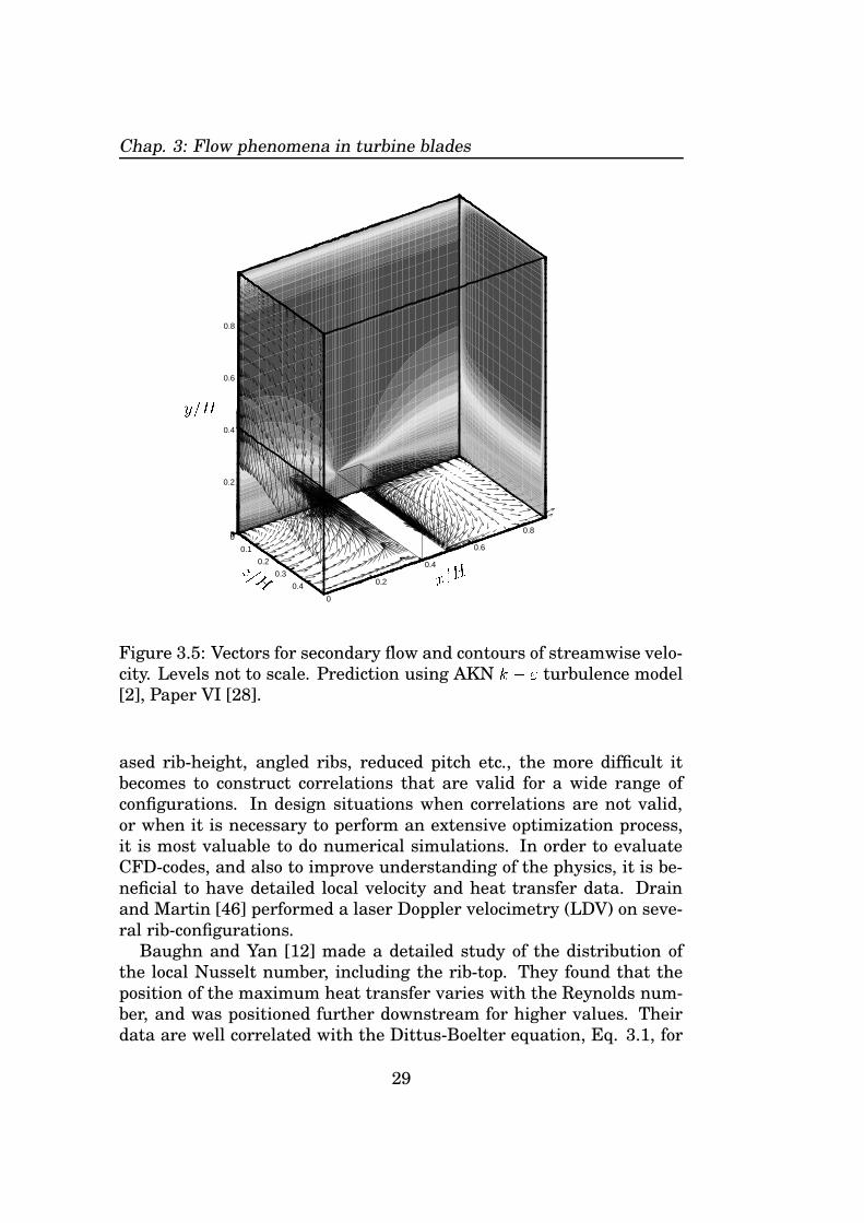
Figure 3.5: Vectors for secondary flow and contours of streamwise velo-city. Levels not to scale. Prediction using AKN � � � turbulence model[2], Paper VI [28].
ased rib-height, angled ribs, reduced pitch etc., the more difficult itbecomes to construct correlations that are valid for a wide range ofconfigurations. In design situations when correlations are not valid,or when it is necessary to perform an extensive optimization process,it is most valuable to do numerical simulations. In order to evaluateCFD-codes, and also to improve understanding of the physics, it is be-neficial to have detailed local velocity and heat transfer data. Drainand Martin [46] performed a laser Doppler velocimetry (LDV) on seve-ral rib-configurations.
Baughn and Yan [12] made a detailed study of the distribution ofthe local Nusselt number, including the rib-top. They found that theposition of the maximum heat transfer varies with the Reynolds num-ber, and was positioned further downstream for higher values. Theirdata are well correlated with the Dittus-Boelter equation, Eq. 3.1, for
29

Jonas Bredberg, Internal Cooling of Gas-Turbine Blades
the two higher Reynolds numbers ( � � � � � � � � � ) howeverthe lower ( � � � � � ) case follows the Reynolds number raised to �� � .In Paper II [26] this Reynolds number effect for rib-roughened channelwas studied using three different types of turbulence model. The ex-perimental data [144] coincide with the behaviour given by Richardson[176] and Sogin [188] behind bluff-bodies, ie.
� � � � � ��� � . The numeri-cal simulations however, for all turbulence models, erroneously followthe smooth duct correlation by Dittus-Boelter [43],[135]:
� � � �� � � � � � � �'& � �(3.1)
In Paper I [23] it was shown that turbulence models that agree wellwith a low Reynolds numbered case, over predicted the heat transferfor a high Reynolds numbered case. A similar behaviour can be dedu-ced from the data presented in [94].
X
Y
Z
2.42.221.81.61.41.210.80.60.40.20
PSfrag replacements
� � � � � �
Figure 3.6: Normalized nusselt number, rib-roughened wall. Predictionusing the AKN �� � turbulence model [2], Paper VI [28].
Kukreja et al. [110] investigated the effect of the spanwise distri-bution on the Sherwood number due to differently angled ribs, and
30

Chap. 3: Flow phenomena in turbine blades
found that the vortical cells produced by the angled ribs produce a verycomplex pattern in the local mass transfer (or equivalent heat trans-fer) which is impossible to correlate to any empirical function. Evenfor orthogonal ribs, a substantial variation of the heat transfer in thespanwise direction is evident, see Fig. 3.6. The results from these andsimilar experiments show the necessity to perform three-dimensionalcomputations. In Paper VI [28] it was however concluded that for ort-hogonally ribs the centerline Nusselt number could still be reasonablyapproximated using a 2D simulation, see further discussion in Section4.5.
Assessment of turbulence and heat transfer models are laborious bythe fact that most experiments only measure heat transfer data, andhence it is impossible to separate the performance of the heat trans-fer model from that of the turbulence model. The detailed study byRau et al. [171] includes both flow field and heat transfer measure-ments, which makes this experiment exceptionally valuable for tur-bulence model evaluation. The case have consequently been used ascomparative data for several numerical simulations: [149],[180], andby the author in Paper VIII [24] and VI [28], see Fig. 3.6.
3.3 Secondary flowsIn most flows it is possible to identify a pre-dominant flow direction –the streamwise. Flow structures, which are not arranged in that direc-tion are normally referred to as secondary flows. These can originateas a result of either geometrical constraints, eg. ribs, or due to impo-sed forces. Prandtl [168] classified secondary flows into two distinctgroups:
1. Generated by inviscid effects.
2. Generated by Reynolds stresses.
The first process, denoted secondary flow of the first kind, is generatedby turning a shear-layer perpendicular to its main vorticity direction.Flow in a channel with a large aspect ratio (wide) can for the center-line be simplified to a two-dimensional flow, with (say) the streamwisedirection along the
�-axis and the wall-normal direction along the � -
axis. Vorticity, defined as
� � � ���� � �������� (3.2)
31

Jonas Bredberg, Internal Cooling of Gas-Turbine Blades
thus exists only in the spanwise direction: �� � ��� � ��� � � � � � � . In order
to produce secondary flow of the first kind for this flow there needs to bea process which generates either a
�- or a � -component of the vorticity
vector. The main re-circulating bubble in a ribbed channel flow is thusnot per se a secondary flow, as the ribs only generate spanwise vorticity,through an increased shearing.
Secondary flow of the second kind develops in corners of a duct,where the cross-stream gradients of the Reynolds stresses generateweak streamwise vorticity, see the predicted cross-section velocity vectorsin Fig. 3.7. DNS’s ( � ��� � � [55], and � ��� � � [80]) and LES’s [152](included as Fig. 3.7(c)) clearly show this type of turbulence inducedsecondary motion. The flow in the cross-stream plane is characterizedby two contra rotating vortices in each corner. Because these structu-res are driven by gradients of Reynolds stresses they cannot be captu-red using an isotropic eddy-viscosity models, as notable in Fig. 3.7(d).The two additional figures in Fig. 3.7 (Fig. 3.7(a) and 3.7(b)) showthe predicted secondary flows using an EARSM [54] with two differentpressure-strain models (SSG [193] and LRR [120]).
Demuren and Rodi [42] made a thorough review of the, at that time(1984), modelling achievements with comparisons to experiments. Thepresent available DNS-data however make it possible for a more fun-damental analysis. Based on their DNS-data [81] Huser et al. conclu-ded that although the basic secondary motion can be captured usingnon-linear models, no turbulence model can accurately predict the tur-bulence characteristic of Prandtls secondary flow of the second kind. Arecent computation by Petterson and Andersson [163] using an RSMwith an elliptic relaxation [48] and the non-linear SSG pressure-strainmodel confirms the problems of accurately predicting these secondaryflows even with the most complex and advanced second-moment clo-sures. Noting the weakness of these structures ( � � � � of the bulkvelocity) the influence of the Reynolds stress induced secondary flow isless important in complex and disturbed flows. In the result sectionit is shown that for rotating rib-roughened channels, where the flowis characterized by large-scale separation and rotational induced se-condary flows, there is only a minor modification by adding non-linearterms (EARSM) to the eddy-viscosity turbulence model. The perfor-mance in a squared duct should thus not be used as an argument forusing Reynolds stress based turbulence models in ducts with ribs.
Contrary to Prandtls secondary flow of the second kind, the secon-dary flows governed by inviscid processes are significantly simpler topredict and also more influential on the flow structure. There are two
32

Chap. 3: Flow phenomena in turbine blades
0 0.1 0.2 0.3 0.4 0.5
0.5
0.6
0.7
0.8
0.9
(a) EARSM-SSG
0.5
0.6
0.7
0.8
0.9
0.5 0.6 0.7 0.8 0.9
(b) EARSM-LRR
0 0.1 0.2 0.3 0.4 0.50
0.1
0.2
0.3
0.4
PSfrag replacements
(c) LES
0
0.1
0.2
0.3
0.4
0.5 0.6 0.7 0.8 0.9
(d) EVM
Figure 3.7: Predicted secondary flow in a square duct. Each sub-figurerepresents one-fourth of the duct. EARSMs are able to capture thegeneral flow structure with eight turbulence induced vortices, while li-near EVMs are unaffected by the corners. EARSM by Gatski and Spe-ziale [54] using either SSG [193] or LRR [120] pressure-strain model.The EVM is the � � � model by Abid et al. [3]. LES results supplied byPallares [151]
33

Jonas Bredberg, Internal Cooling of Gas-Turbine Blades
mechanism that drives the generation of secondary flows of the firstkind, either: 1) a pressure gradient or 2) an imposed body-force inthe cross-stream plane. The latter could be the Coriolis force due torotation, or buoyancy as a result of uneven heating. The former, ie.pressure gradient induced secondary flows, is generated by geometri-cal conditions, eg. ribs as discussed above.
In rib-roughened channels, the void behind the rib generates a down-ward motion within the re-circulating region. This motion, accompa-nied by the no-slip condition along the side-walls, will generate a circu-lar motion with two opposite rotating cells [76]. The downward flow inthe center of the duct is seen in Fig. 3.5. In the same figure a transver-sal motion along the bottom wall is also noted. This is the result of thespanwise difference in pressure due to the ribs, which for angled ribsis further amplified. When the ribs are arranged in a V-configuration,the highest pressure is found in the center of the duct, at any givenstreamwise location. Kukreja et al. [110] found that such an arrange-ment further enhances the strength of these cells, with a significantre-distribution of the heat transfer pattern as a consequence.
3.4 Bends – curvatureThe internal cooling systems of gas turbine blades are commonly ar-ranged in a serpentine manner, with a number of rib-roughened ductsconnected using sharp � � � bends. Motion within a bend will generatea centripetal acceleration which is balanced by an opposing pressuregradient. To a first order approximation the following condition is ap-plicable:
� ���& � � � �� (3.3)
where�
is the streamwise velocity. In bends with a low curvature1, thepressure gradient will vary linearly from the inner- to the outer-radii.High momentum fluid in the center tends to drift outwards in accor-dance with the above relation. Continuity requires that the outwardmotion in the center of the duct, is balance by a reverse flow along thewalls, where the streamwise velocity is lower and hence the centrifugalforce is less. A circular motion in the cross-stream plane is thereforegenerated. The flow out from a bend is characterized by two opposing
1The curvature is the inverse of radius
34

Chap. 3: Flow phenomena in turbine blades
rotating cell, with vorticity in the streamwise direction. A parameterthat measure the curvature effect, relatively to the viscous effect is theDean number. The curvature induced cells are consequently also refer-red to as Dean cells.
The stability of the flow in a bend can be studied through a perturba-tion analysis. If a fluid lump along the inner radius (convex) is slightlydisplaced outward into a high-velocity region, the lump with a nowunbalanced low momentum will return, due to the imposed pressuregradient, to its original position. Such a flow is denoted a stable flow.The opposite condition is true for the outer (concave) side, and hencethis side is unstable. A measure of the degree of stability is given bythe Dean number. Exceeding a critical Dean number results in the de-velopment of instabilities in the flow, as given by Rayleighs criteria, see[154]. An analog is found in boundary layer flows over concave walls,for which Gortler vortices is produced if the centrifugal instability islarge enough.
Flows in curved ducts and the associated stability problems havebeen studied by numerous peoples including the great turbulence rese-archers Prandtl, van Karman, Taylor. A recent investigation [29] usingLES clearly shows the complex multiple cells in the cross-stream planewithin the bend. Although fundamentally the secondary flows in cur-ved ducts are govern by the inviscid centrifugal force, the stability ofthe system is based on the viscosity and hence the level of turbulentviscosity for turbulence modelling is of most importance. The first topropose a model to account for turbulence modifications due to curva-ture was Prandtl [169]. He proposed to add a correction to the mixinglength, based on a local dimensionless curvature parameter:
� � �� � � � � (3.4)
Bradshaw [18] used the similarly defined Richardson number, see Eq.2.13, to modify the turbulent length scale. In standard two-equationmodels ( � � � , � � � ), the turbulent length scale is not given explicitly andhence such a modification is not applicable. Launder et al. [119] ins-tead introduced a Richardson number modification in the � -equation.Wilcox and Chambers [210] argued that the modification should be ap-plied to the turbulent kinetic energy, since streamline curvature makesa redistribution among the Reynolds stresses. Under de-stabilizingconditions the wall-normal component is amplified accompanied by areduction of the streamwise component. The opposite is valid for astable, convex side. It is thus not surprising that isotropic EVMs have
35
Jonas Bredberg, Internal Cooling of Gas-Turbine Blades
limited capability to correctly assess the complex secondary flows ina bend as shown in [118]. Although the Wilcox-Chambers model maysound plausible, the level of turbulence energy is markedly different onthe concave and convex side of a bend, and hence their strategy for ac-hieving improved predictions, through only re-distribution among thestress components is questionable. In the result section (and also [19])more realistic profiles for the turbulent kinetic energy is given usinga Richardson number modified � -equation than with the Wilcox andChambers � -equation modification, albeit for rotating flows. More re-cent attempts to improve predictions in curved duct have all focusedon the � -equation [74], [182]. Numerical simulations using RSM [133]have shown that even these models benefits from a modification to thelength scale for highly curved ducts.
3.5 RotationIn the study by Bradshaw [18] it was shown that the effect of an im-posed rotation can be treated in analog to streamline curvature. Theextension to include buoyancy effect due to heating was also asses-sed, however such an analog can only be a rough approximation, asthe driving mechanism differs. The connection between rotation andcurvature can easily be demonstrated, and in cases when the rotationaxis is parallel to the curvature-axis these two process will genera-ted similar secondary motions. Neglecting buoyancy and wall-effectsthe only remaining rotational induced force, will be the Coriolis-force( � � �
), which corresponds to the centripetal force (� � � � ) for a curved
surface. In a bend the streamwise velocity could be approximated by alinear variation from the inner to the outer wall with a slope of
� � � .In a duct exposed to system rotation a similar behaviour is present,although the skewness of the velocity profile is given by the magnitudeof � �
(referred to as the background vorticity in [100]) instead of thecurvature parameter,
� � � . In inviscid regions, where wall effects arenegligible, the DNS by Kristoffersen and Andersson [109] confirms thevalidity of this relation. In experiments, the inevitably introductionof spanwise walls disturb the clean results achievable in a DNS. Ina recent high fidelity LES (DNS-like) by Pallares and Davidson [152]the interaction of Prandtls secondary flow of the second kind (stress-induced) with those of the first kind (rotational-induced) is studied. Itis apparent that for increasing rotational numbers, the corner vorticesare suppressed and that the cross-stream secondary motion is mainly
36

Chap. 3: Flow phenomena in turbine blades
0 0.25 0.5 0.75 10
0.1
0.2
0.3
0.4
0.5
0.6
0.7
0.8
0.9
1
PSfrag replacements
���
� � �
Figure 3.8: Cross-section velocity vectors (left) and contours ofstreamwise velocity (right). Rotation around � -axis: ��� � � � � . LES[152].
govern by the Coriolis force, see Fig. 3.8 and compare with Fig. 3.7(stationary).
The equations governing fluid motion are, as discussed in Chapter2, the Navier-Stokes equations. The additional terms, due to rotation,are the centrifugal and Coriolis accelerations, which translates into thefollowing body-forces:
� � � � ��
�����
���� � � � � ��
(3.5)� �� � � � � �
���� � � ���(3.6)
These terms are generally found on the RHS of the NS-equation. Forincompressible flow, or a flow with negligible buoyancy, the centripetalforce is conservative and can be assimilated into a reduce pressure gra-dient [59]. The contribution of the Coriolis force is, as obvious from thedefinition, perpendicular to the rotation axis and placed in the cross-stream plane (
��� �). In a rotating square duct, the cross-stream flow
will be aligned with the Coriolis force in the core of the duct, for which
37

Jonas Bredberg, Internal Cooling of Gas-Turbine Blades
the streamwise velocity, and hence the Coriolis force is strongest. Alongthe side-walls a reverse flow is found, as dictated by continuity, see Fig.3.8.
PSfrag replacements
�
� �
Coriolis
Coriolis
Curvature
�
� �
Figure 3.9: Rotational and curvature induced secondary flows.
A connection between the rotation and curvature induced secondaryflows can be visualized in a rotating U-bend, Fig. 3.9. With
�as the
streamwise component� � � � � � � � � � and a rotation around the � -
axis� � � � � � � � � � � , the Coriolis force
� �� ��� � � � ��� � � is parallel to the� -axis, and generates a secondary flow in the cross-stream plane, � � � .The curvature effect, as discussed in the previous section, produce asimilar secondary motion within the bend and in the downstream leg,as shown in Fig. 3.9.
The analog between streamline curvature and rotation can be exten-ded to stability analysis. When the main Coriolis component is perpen-dicular to the surface a perturbated fluid particle will either be forcedback, or driven away from the surface, dependent on the direction ofthe Coriolis force. If the rotational induced acceleration (opposite to
38

Chap. 3: Flow phenomena in turbine blades
the force) is directed into the surface the flow is stabilized. As poin-ted out previously a stabilized boundary layer suppress turbulence,and can under strong rotation even laminarize. The reverse is truefor the de-stabilizing surface (impinging secondary flow), for which theturbulence is enhanced. In a square duct the stress-induced corner-vortices are significantly reduced for increasing rotational number onthe stable side, see Fig. 3.8. The formation of Taylor-Gortler vorti-ces, similar to those for a convex surface on the unstable side of theduct, was shown in [152]. An accurate numerical simulation of rota-ting flows thus necessities a higher-order turbulence model, althoughthe main vortices, governed by the inviscid Coriolis force, is capturedusing even the simplest flow model.
3.6 Review, experiments and numerical si-mulations with reference to turbine bladeinternal cooling.
The importance of improving the cooling of gas turbine blades haveseen an increasing demand of, initially experimental evidences, andnow well validated numerical methods for use as optimization tools.The effect of variating rib-sizes, Reynolds number etc. have been docu-mented in both numerical simulations and experimentally.
Although the many merits of experimental evidence, there is a pro-blem that should be recognize when performing experiments: it is verydifficult to achieve conditions which enable measured data to be de-pendent on only a single parameter. In many investigations the datais obscured by slight perturbations in Reynolds number, different hea-ting, rotation number etc. These unknowns add up to a level of uncer-tainty in the measured data, which should be considered when makingcomparisons to the predicted result. In numerical simulations on theother hand it is very easy to ensure an exact Reynolds number or thatthe flow is incompressible, or that the temperature behave as a passivescalar etc., all conditions which can only be an approximation of thereal world. It is thus important that both measurements and predic-tions are made under as identical conditions as possible, to enable anaccurate evaluation of turbulence and heat transfer models. The ap-pearance of Direct Numerical Simulations have had a great impact onturbulence modelling as these numerical ’experiments’ could be com-pletely controlled, with known boundary conditions. These simulations
39

Jonas Bredberg, Internal Cooling of Gas-Turbine Blades
also provide a wealth of information. DNS are however very computa-tional costly, and only some fundamental flows can be studied with thisapproach. In other cases, such as the internal cooling systems of a gasturbine blade, one needs to rely on data from experiments.
3.6.1 Experiments:Many of the early investigations were made to evaluate the concept ofrib-roughened ducts for enhancing cooling performance. Initially thesize of the ribs could be maintained relatively small, � � � � �� � , as thecooling needs was much less than today. Because of this it was possibleto compare rib-roughness with an equivalent sand-grain roughness,
� �� .The latter has been studied extensively by Nikuradse [146] and is welldocumented. The experiments were thus aimed at constructing corre-lations between rib-size, �
� � , Reynolds number, � � , and the frictionfactor,
�, similarly to those given by Nikuradse. The heat transfer can
then be computed for different fluids using correlations based on thePrandtl number,
� &, and the previously achieved friction factor,
�, as
shown in [204], [102]. An early compilation on rib-roughened circulartubes is found in [204].
It was however soon realized that an increased heat transfer per-formance was needed. The simplest way to achieve this is to increasethe size of the ribs. This however also increases the pressure drop. Inorder to enhance the heat transfer performance2 the effect of differentrib cross-sectional shapes and skewed ribs were investigated in Han etal. [63], [65], [67]. It was shown that the effect of ribs on the oppositewall also modifies the results when the rib-to-channel-height is large.In other studies, [62], [64], the aspect ratio of the channel was varied.Constructing correlations which incorporate all these parameters havenow become a rather delicate business. In subsequently studies [66],[67] it was also concluded that it is impossible to curve-fit such a wealthof data. A recent and comprehensive compilation of the effect on heattransfer from a variety of rib-configuration could be found in the vanKarman Lecture series given by Taslim [196], or alternatively, but lesscomplete [197].
Although the importance of understand rib-roughened channels, thereare other flow phenomenas that appear in internal cooling ducts of tur-bine blades, such as rotation, curvature and buoyancy. In the abovediscussion on rotation, the effect of buoyancy was neglected, to simp-
2Heat transfer performance also consider the friction coefficient/pressure drop.
40

Chap. 3: Flow phenomena in turbine blades
lify the treatment of the already severely complicate flow structure.Experiments made with a bearing to the gas turbine industry, will na-turally focus on heat transfer rate, and hence the buoyancy effect canonly be neglected for certain special cases. In most studies of rotatingducts the measured data is thus affected by a buoyant force, as are eg.[68], [111], [16]. Generally there are however several effects present,such as rotating channels with roughened walls [139]. U-bends (ie. in-cluding curvature effect) with roughened walls are studied in [52], [88]and rotating U-bends in [31], [83], [89]. [127], [138], [201] and [202].
Experiments that simulate conditions in a turbine blade need to su-perimpose all these effects (rotating, rib-roughened U-bends) see eg.[157], [158] and [50]. In the latter two the effects of different model ori-entation was also included. Other investigations [90], [98], [216] havestudied skewed ribs. Most experiments only measure heat transfer, ho-wever [87] also gives accurate flowfield data using LDV. The value ofsuch experiments for the assessment of turbulence models, should beemphasized. Reviews on experimental investigations are given in [78]and [79].
3.6.2 Numerical simulations:Apart from some rather academic case, the complexity of each of theabove phenomena (rib-roughened walls, streamline curvature and ro-tation) necessarily means that a three-dimensional simulation must beperformed. Due to the tremendous advances in computational powerlately, the most interesting numerical simulations are hence fairly re-cent.
A review on numerical simulations is given by Prakash and Zerkle[166]. Their contribution was a computation of a rib-roughened rota-ting duct with cyclic streamwise boundary conditions to reduce compu-tational costs. Furthermore the buoyancy-centrifugal effect was neg-lected, for simplicity. The turbulence model used was the ��� � witheither wall-functions or a zonal approach for the wall treatment. Pra-kash and Zerkle inferred that a number of refinement were necessary,however without any experimental data their conclusions could only bebased on phenomenological discussions.
Rib-roughened channels:An early and valuable investigation was made by Liou et al. [129] whoperformed both heat transfer measurements and numerical simula-
41

Jonas Bredberg, Internal Cooling of Gas-Turbine Blades
tions using a � � � algebraic stress turbulence model. The case studiedwas the one previously measured by Drain and Martin [46] using LDV.In the 7:th ERCOFTAC Workshop the result from Liou et al. was usedto evaluate CFD-codes and turbulence models. Significantly differentheat transfer results were presented at the workshop dependent onused models, see eg. the authors contribution: [22]. Two of the groups,re-visited the test-case using more advanced turbulence models. Theextension using an EARSM formulation [3] of the � � � turbulence mo-del did however little to improve the result, see Paper I [23]. Manceauet al. [134] applied the � � � � � � � turbulence model [47] with impres-sive results for the floor between the ribs. The heat transfer around therib, was however not accurately captured although different boundaryconditions were used.
Another test case in the workshop was a 3D rib-roughened chan-nel with ribs placed on two opposite walls in a staggered arrangement.However only a single group contributed with any predicted data. Theresult using a zonal DSM and a LRN � ��� turbulence model was laterpublished [84] and [95]. The mean quantities were accurately predic-ted, however heat transfer was under predicted using the zonal-EVM.The LRN � � � necessitates the inclusion of a Yap-correction [212] toyield acceptable heat transfer rates. Similar conclusions, for the samemeasurement data [87], [88] were drawn by the author [19], when com-paring a zonal � � � with a � � � and EARSMs. A subset of this data isincluded in Section 5.2. Ooi et al. [150] also studied this case, with the� ��� � � � � turbulence model, and achieved good agreement.
Other interesting numerical studies on rib-roughened channels areeg. the combined measurements and simulations using both a stan-dard and a non-linear ��� � turbulence model in [5]. The predictedNusselt number different only marginally dependent on the selectedturbulence model. A comparison between wall function based turbu-lence models for a single rib was performed in [4]. Abdon and Sunden[1] investigated different rib-shapes similar to that of [63] and foundthat de-graded ribs (with rounded edges) yield superior heat transfer tofriction ratio. The only LES (although rather coarse) which has simu-lates these configurations is the one made by Ciofalo and Collins [36].A notable qualitatively improvement in the predicted Nusselt numberwas found when comparing the LES with a standard � � � turbulencemodel. The treatment of ribs using spectral methods however pose asevere obstacle in DNS and LES studies. A way to circumvented thiscould be, as done in the DNS by [141], through simulating the ribs withsource and sink terms in the momentum equations.
42

Chap. 3: Flow phenomena in turbine blades
Curvature:In the case of predicting curvature there is a distinct additional model-ling complexity if the flow separates as a result of the adverse pressuregradient due to the bend. In simulations with only a moderated curvedbend, there have been attempts to predict the flow without any length-scale corrections, even though their inclusion is theoretically well foun-ded as discussed in Section 3.4. In [13] and [34] it was concluded that itis essential to resolve the near-wall region in curved ducts, as the pre-dictions using the PSL and wall-functions, respectively, were inferiorto that using a refined mesh and employing the mixing-length model.Using the same case, Iacovides et al. [92] employed a differential stressmodel (DSM), with and without modification to the � -equation. The re-sults with the DSM were similar to those achieved earlier, using ASM,however with detectable improvements in certain regions.
For stronger curvature, as the case studied by Cheah et al. [31]( � �
� � � � � � ) the flow separates within the bend, and hence morestringent conditions is imposed on turbulence modelling. In separatedregions the mixing-length hypothesis fails and hence it is necessary toemploy more elaborated schemes in the near-wall region. In Iacovideset al. [93] a comparison was made between using different wall treat-ments in connection with an ASM. The near-wall region was resolvedeither using an one-equation model [211] ( � determined from a prescri-bed length-scale) or a two-equation based turbulence model ( � givenfrom its transport equation). For all models the separated region wasinaccurately predicted, with only a slight improvement using the fullLRN-version of the model. In a subsequently study [145] it was conclu-ded that for heat transfer predictions a LRN turbulence model is pre-ferable to a zonal model in the near-wall region. The separation washowever not well predicted using any of the turbulence models. TheIacovides group have continued with a number of numerical simula-tions using wall-functions [148]. That study shows that the core model(EVM vs RSM) is of importance for the heat transfer, even though thenear-wall is rudimentary modelled.
Luo and Lakshminarayana [132] made a similar comparison for ahigh Reynolds number U-bend of strong curvature. To reduce compu-tational costs the simulations were restricted to a plane 2D duct andsimilarly to previous computations the zonal technique was employedwhen resolving the near-wall region. The result using an RSM was su-perior to the other turbulence models ( � � � , non-linear � � � and ARSM)
43

Jonas Bredberg, Internal Cooling of Gas-Turbine Blades
with the linear � ��� performed the worst. In a subsequent paper [133]they introduced length-scale modifications by [119] and [182] to theirRSM and achieved significant improvements on the concave surface.Bauer et al. [11] compared a number of higher-order turbulence mo-dels (non-linear EVMs: [38], [183] and EARSM [54]) with the standard� � � [101] and the LRR RSM [120], for the same high Reynolds num-ber case. They found similarly to Luo and Lakshminarayana that the��� � turbulence model is inadequate. They concluded that althoughimproved results were achieved with the non-linear turbulence models,the cross-velocity coupling in the momentum equation can lead to sol-ver divergence, and hence they used truncated versions of the models.Methods to improve numerical stability, other than simply truncatingthe turbulence models are discussed in [69]. In these simulations theassumption of a 2D flow and the use of an one-equation model [132], orwall functions [11] to bridge the near-wall region may however influ-ence the result, particularly in separated regions.
Unpublished results by the author from numerical simulations inthe Cheah et al. [31] U-bend using unmodified LRN two-equation mo-dels indicate the need for length-scale corrections, especially when pre-dicting heat transfer within the bend region. The results presented inPaper VII [25], although for a rib-roughened U-bend, also shows se-vere discrepancies in this region. Another U-bend simulation usingLRN turbulence model was performed by Rigby et al. [178]. They usedthe � � � turbulence model by [208] and achieved reasonable accuracyeven for heat transfer.
Rotation:In the 7:th ERCOFTAC workshop a two-dimensional like (high aspectratio) rotating flow was used to evaluate turbulence models. DNS-datafor this flow was supplied by [109]. The result from the workshop sho-wed, not surprising, that the isotropic EVMs are unable to capture theincrease/decrease of turbulent kinetic energy on the unstable/stableside. Better agreement were achieved when non-linear EVMs, EARSMand RSMs were used, although discrepancies still persisted in the near-wall region, especially on the stabilizing side. Most turbulence modelsover-predicted the suppression of turbulence, with a too early flow la-miniarisation. In Chapter 5 it is shown that notable improvements canbe achieve if rotational modified length-scale corrections – in analog tothose used for streamline curvature – are applied. It has been shown[150] that even the ���� � � � � model necessitates rotational modifi-
44

Chap. 3: Flow phenomena in turbine blades
cation to capture the skewed velocity profile in rotating ducts.It should be noted that even RSMs, which have an exact formulation
of rotational induced stresses, benefit from these length-scale correc-tions as the � -equation is affected by rotation. In addition the Reynoldsstress equations are not frame invariant, and hence an imposed acce-leration alters these equations similarly to the NS-equations. Launderet al. [123] proposed a correction for this effect through a modifiedpressure-strain model. For non-linear EVMs and EARSM the rota-tional induced stresses can be included through a modified rotationaltensor,
� ��� [54], [183], [203]Howard et al. [77] compared predictions with and without length-
scale correction for both a high- and low-aspect ratio channel. Theyconcluded that any rotational modification to the turbulence model wasless important for low-aspect channels. A similar conclusion is givenby the presented results in Chapter 5, where rotational induced turbu-lence modification are significantly more important in the 2D channelwhen compared with the 3D squared channel. Although it is not pos-sible to make a proper comparison between the two test cases, as thelatter channel is also equipped with ribs, the conclusion from 3D flowis of a higher engineering interest as that is more in line of real lifeproblems. It is thus not surprising that many numerical simulationsdo not bother to incorporate these corrections.
A review of theoretical and experimental achievements for rotatingchannels could be found in [165]. In their paper they used a � � �turbulence model to simulate a flow affected by both buoyancy androtation and achieved acceptable agreement without any turbulencemodel modification. Their use of wall-functions for the near-wall treat-ment would anyhow have drastically reduced the likely improvementsof such a modelling effort.
Numerical simulations of combined effects:Judging from the above discussions on the problems of achieving a highdegree of fidelity for the different flow phenomena it is not surprisingthat in cases when combined effects are present, less attention is givento theoretical consideration and more to practical issues. A significantrestriction when computing eg. rotating U-bends is the need for a 3Dsimulation, and hence both computing time and resources increasestremendously. In many cases one is restricted to a single mesh and asingle model to evaluate the configuration, not an ideal situation whenperforming numerical simulations. Furthermore, the computational
45

Jonas Bredberg, Internal Cooling of Gas-Turbine Blades
demands necessitates as many simplifications as possible, such as theapplication of wall function based � ��� turbulence model by Dutta etal. [49], [51]. The same rotating (smooth) U-bend case3 was studied byBonhoff et al. [14] and Iacovides et al. [93] using higher-ordered turbu-lence models (ASM and RSM respectively). Similar to previous studiesby the UMIST-group (Launder, Iacovides) the latter study employed aone-equation model in the near-wall region, while [14] used standardlogarithmic wall function in a commercial code. For a lower Reynoldsnumber case, � � � � � � , Stephens and Shih [195] was able to use aLRN � � � turbulence model on a ��� � � � � mesh for their compressiblesimulation. The result was in good agreement with the measured databy [201] and [202].
Even larger meshes are needed for U-bends with rib-roughened walls.The author estimated that the required number of nodes on a well re-solved mesh for the case studied in Paper VII amounted to � � � � . Allthe following computations; [15], [85], [96], [126] [177], and [194] havethrough a number of simplifications been able to reduce this require-ment by a magnitude, including the author in Paper VII [25] where thesimulations was made on ��� � � � � mesh.
A case investigated by several of the above authors is the one studiedby [98] and [202]: � � � � � � , ��� � �� � � with staggered ribs skewed at� � � angle to the streamwise direction. In Bonhoff et al. [15] the numberof nodes were reduced through employed wall-functions in their com-putation using � ��� and Reynolds stress turbulence models. The com-mercial code FLUENT was able to predict the trends correctly whencomparing smooth with ribbed channel, and stationary with rotating,although the magnitudes of the changes were inaccurate. In additionthe overall difference between the predicted and measured heat trans-fer levels was greater than desired. Better agreements were achievedby Stephens et al. [126] and [194] for the same case through employingLRN ��� � turbulence model in [194] and the SST turbulence modelin [126]. The usage of a LRN turbulence model however significantlyincreases the number of nodes, and even though the total number ofribs (in all 20) was reduced compared with the experiment they stillneeded � � �
� � � � � � � � � ��� � � node points. They made however onlyrudimentary comparisons to measured data, and not for the importantribbed case. In Jang et al. [96], a reduction in the number of nodes wasaccomplished through restricting the computational domain to a singleleg of the U-bend. Their grid-refinement study with the used LRN ver-
3Measurements by [31].
46

Chap. 3: Flow phenomena in turbine blades
sion of a RSM showed a significant difference ( � �� ) in the predictedheat transfer between a mesh with � � � � � nodes and one with
� � � � �nodes in the cross-section plane. Further refining the mesh to � �
� � �
nodes gave a difference of� � . Using the � � � � � � � � � � � � � � �� mesh
they achieved a comparable good agreement with measured data. Theprediction, similarly to the experiment, showed a significant changein the heat transfer levels due to the rotational induced Coriolis force,with a reduction of up to
� � on the leading face, and an increase onthe trailing face by up to � ��� .
In a similar case [155], however with normal ribs, and at a lowerReynolds number ( � � � � � � ) Rigby [177] employed the LRN � ���turbulence model [208]. A satisfactory agreement with measured datacould however only be achieved through a modification to the boundaryfor � as proposed in [136], in connections with the rough-wall modifi-cation by Wilcox [207]. It was found that the predicted heat transfer(or actually mass transfer) was significantly influenced by the assu-med wall-roughness and varied by a factor of three between the usedroughness values. With the assumption of a smooth wall the flow didn’tre-attach in-between the ribs, and hence the turbulence level and con-sequently the mass transfer was severely under predicted. Improvedresults were achieved with the rough wall, however the trends in theupstream and downstream leg were not captured.
The ribbed case equivalent to the smooth case studied in [31] wasinvestigated by Iacovides et al. (experimentally: [87], [88] and nume-rically [85]) and also by the author, Paper VII [25]. Iacovides couldreduce the computational requirement4 through adoption of zonal tur-bulence models ( � � � and RSM) and the usage of a bounded QUICKdiscretization scheme. The results showed the advantage of using theRSM in regions of flow separation, however the main flow features werestill captured by the ���� model. In the case of negative rotation, withthe rotation and curvature induced force opposed each-other, the agree-ments were significantly reduced as compared to the case with positiverotation. The cause may be the inability of zonal models to accuratelyasses these phenomenas within the near-wall region. Heat transferpredictions were not included in the study.
The author, in Paper VII [25], made a numerical study of the samecase, � � � � � � , ��� � �� � , with normal ribs arranged staggered,using a modified LRN ���� turbulence model. The baseline model was
4The total number of nodes, with symmetry in the curvature-plane, were: �������� ���� �� ���������
47

Jonas Bredberg, Internal Cooling of Gas-Turbine Blades
developed in Paper VI [28] with the coarse mesh modification introdu-ced in Paper VIII [24]. It was discovered during the simulations thatthe cross-diffusion terms was numerically problematic and an additio-nal modification was necessary to limit these terms. The result wasboth enhanced stability of the code and improved prediction of the heattransfer. Similar to previous studies discrepancies were found withinthe U-bend and immediately downstream the bend, however overallboth the trends and the magnitude were in good agreement with mea-surements.
48

Chapter 4
Numerical Considerations
The CFD-code used in this thesis is presented. The con-sequences of numerical approximations and computationalsimplification are discussed. Mesh dependency problems inregards to turbulence models and geometrical configurationsare addressed.
4.1 Numerical MethodThe solution method used in this thesis for the governing equations(Navier-Stokes equations), is the Finite Volume Method (FVM). Usingthis method the particular computational domain is divided into a num-ber of control volumes. The differential equations are discretized ontothe computational mesh and numerically integrated over the controlvolumes. The set of equations are then solved iteratively until a con-vergence criteria is reached.
For these computations the incompressible FVM-code CALC-BFC[41] is used. There is a selection of discretizing schemes: hybrid, cen-tral, van Leer [199] or QUICK [125]. The governing equation for aspecific variable,
�, are after discretization expressed as:
� # � # ������
� ��� � ��� � � (4.1)
where � are the coefficients from the convective and diffusive terms.Index � represents the nodal point and ��� the contribution from theneighbouring nodes. Source terms in the governing equations are in-cluded in � . In CALC-BFC this equation system is solved iterativelyusing a Tri-Diagonal Matrix Algorithm (TDMA). In order to improve
49

Jonas Bredberg, Internal Cooling of Gas-Turbine Blades
the diagonal domination in the TDMA solver, the source terms in thegoverning equations are added to the left-hand side if they are negativeand on the right-hand side otherwise.
For incompressible flows the pressure needs to be carefully treatedas the equation of state, � � � � � , is not suitable to use. In CALC-BFC the SIMPLE-C1 [45] algorithm is used to deal with the velocity-pressure coupling.
The code uses Boundary-Fitted-Coordinates (BFC), with the nodesand grid points located in a non-staggered (ie. co-located) configura-tion. This procedure can induce a so-called checker-board solution,due to the velocity-pressure coupling. In CALC-BFC, as in many ot-her CFD-codes, the Rhie-Chow [175] interpolation is used to smoothnon-physical oscillations, arising from this type of grid arrangement.
4.2 Discretizing Schemes and Mesh Depen-dency
To discretize the diffusion terms CALC-BFC uses the central differen-cing scheme. In the numerical simulation performed within this thesisthe convective terms are discretized using either the hybrid, or the vanLeer scheme. It should be noted that the popular QUICK scheme isunbounded, which could lead to numerically stability problems if notcare is taken. The hybrid and van Leer schemes on the contrary arebounded. In this work the pre-dominant choice has been the van Leerscheme.
The hybrid [191] scheme selects, dependent on the local Peclet num-ber (
� ��� � ), whether an upwind or a central differencing approach isused. The order of accuracy for the hybrid scheme is between one andtwo.
In the van Leer [199] scheme the following algorithm is used:�� �
���if � ��� � � ��� � ��� � � � ��� � ��� �
�� �
��� � � ��� � ��� � � ��� � ��� �� ��� � ��� � otherwise
(4.2)
where � � � � �are the west (upstream), point and east (downstream)
nodal values, and � is the approximated east face value. The van Leerscheme is second-order accurate, except at local minima.
1SIMPLE-C is a slightly modified extension of the SIMPLE [160] algorithm.
50
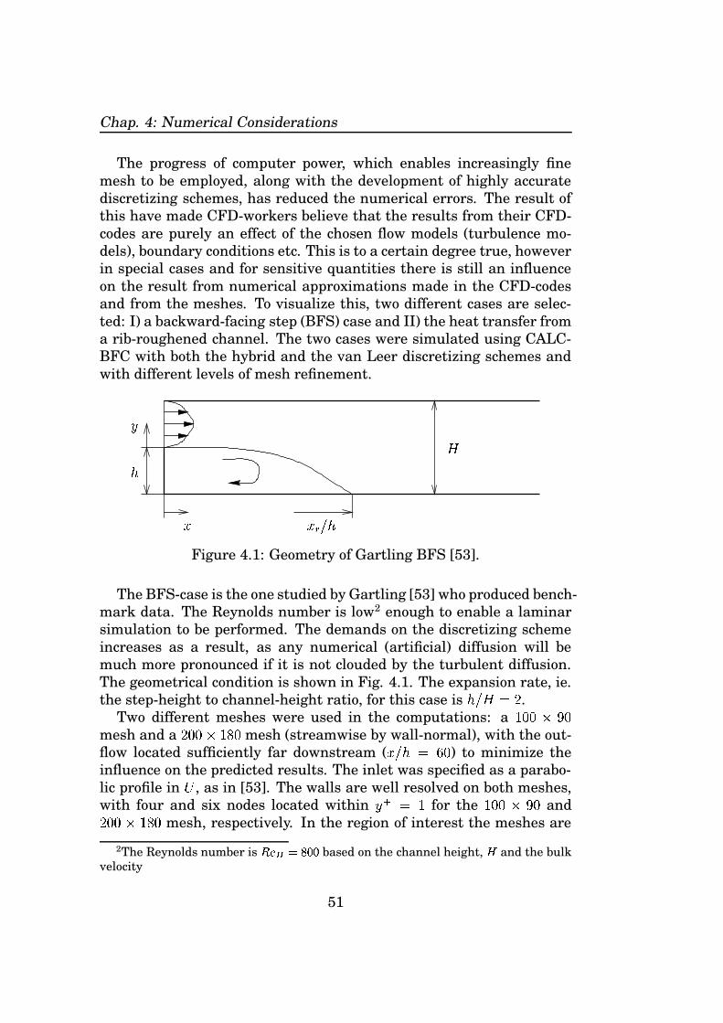
Chap. 4: Numerical Considerations
The progress of computer power, which enables increasingly finemesh to be employed, along with the development of highly accuratediscretizing schemes, has reduced the numerical errors. The result ofthis have made CFD-workers believe that the results from their CFD-codes are purely an effect of the chosen flow models (turbulence mo-dels), boundary conditions etc. This is to a certain degree true, howeverin special cases and for sensitive quantities there is still an influenceon the result from numerical approximations made in the CFD-codesand from the meshes. To visualize this, two different cases are selec-ted: I) a backward-facing step (BFS) case and II) the heat transfer froma rib-roughened channel. The two cases were simulated using CALC-BFC with both the hybrid and the van Leer discretizing schemes andwith different levels of mesh refinement.
PSfrag replacements
��� �
�
�
�
�
Figure 4.1: Geometry of Gartling BFS [53].
The BFS-case is the one studied by Gartling [53] who produced bench-mark data. The Reynolds number is low2 enough to enable a laminarsimulation to be performed. The demands on the discretizing schemeincreases as a result, as any numerical (artificial) diffusion will bemuch more pronounced if it is not clouded by the turbulent diffusion.The geometrical condition is shown in Fig. 4.1. The expansion rate, ie.the step-height to channel-height ratio, for this case is
� � � � � .Two different meshes were used in the computations: a � � �
mesh and a � � � � mesh (streamwise by wall-normal), with the out-flow located sufficiently far downstream (
� � � � � ) to minimize theinfluence on the predicted results. The inlet was specified as a parabo-lic profile in
�, as in [53]. The walls are well resolved on both meshes,
with four and six nodes located within � � � � for the � � � and� � � � mesh, respectively. In the region of interest the meshes are
2The Reynolds number is ����� � ��� based on the channel height, � and the bulkvelocity
51

Jonas Bredberg, Internal Cooling of Gas-Turbine Blades
un-stretched in the streamwise direction, and only gently stretched inthe wall-normal direction, with a maximum ratio, located at the wallsof 4% and 1%3, respectively.
The discretizing schemes are compared for the predicted streamwise(�
), and the cross-stream (�
) velocity profiles at� � � � � . This station
is located immediately downstream the re-attachment point, at��� � �
��� � (benchmark data).
−0.5 0 0.5 1 1.5 2 2.5−0.5
−0.4
−0.3
−0.2
−0.1
0
0.1
0.2
0.3
0.4
0.5
PSfrag replacements
� � �
� � � �
Gartling [53]vL, � � � � H, � � � � vL, � � � H, � � �
Figure 4.2:�
-velocity at� � � � � , BFS. Prediction using: Hybrid (H)
and van Leer (vL) discretizing schemes.
It is shown in Fig. 4.2 that the hybrid scheme is rather sensitive tothe used mesh, while the van Leer scheme predict identical profiles forboth meshes. The hybrid scheme is even for the refined mesh unableto accurately estimate the streamwise velocity. The discrepancies forthe
�profile is even more pronounced, see Fig. 4.3, with the van Leer
scheme on the fine mesh is the only simulation which produced an ac-ceptable accuracy.
The rib-roughened channel is the one studied experimentally by Rauet al. [171]. The Reynolds number based on the bulk velocity is � � � �
3The stretch-rate is defined as the ratio of the cell-heights of two neighbouringcells: ��� ������� �� �
52
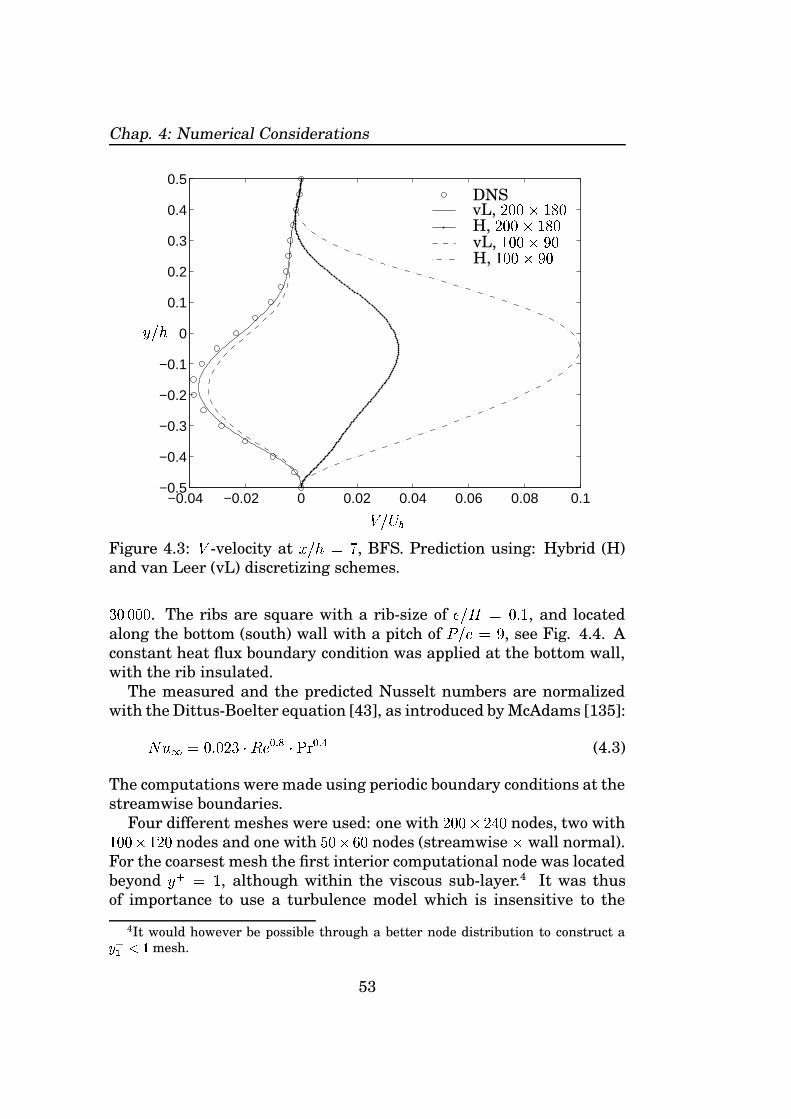
Chap. 4: Numerical Considerations
−0.04 −0.02 0 0.02 0.04 0.06 0.08 0.1−0.5
−0.4
−0.3
−0.2
−0.1
0
0.1
0.2
0.3
0.4
0.5
PSfrag replacements
� � �
� � � �
DNSvL, � � � � H, � � � � vL, � � � H, � � �
Figure 4.3:�
-velocity at� � � � � , BFS. Prediction using: Hybrid (H)
and van Leer (vL) discretizing schemes.
� . The ribs are square with a rib-size of ���� � �� � , and located
along the bottom (south) wall with a pitch of� �
� � � , see Fig. 4.4. Aconstant heat flux boundary condition was applied at the bottom wall,with the rib insulated.
The measured and the predicted Nusselt numbers are normalizedwith the Dittus-Boelter equation [43], as introduced by McAdams [135]:
� ��� �� �� � � � � � � � � ��� � � (4.3)
The computations were made using periodic boundary conditions at thestreamwise boundaries.
Four different meshes were used: one with � � � � nodes, two with� � � � nodes and one with � � � nodes (streamwise
�wall normal).
For the coarsest mesh the first interior computational node was locatedbeyond � � � � , although within the viscous sub-layer.4 It was thusof importance to use a turbulence model which is insensitive to the
4It would however be possible through a better node distribution to construct a� ���� � mesh.
53

Jonas Bredberg, Internal Cooling of Gas-Turbine Blades
PSfrag replacements
� �
���C
YC
LIC
CY
CL
IC
Figure 4.4: Geometry, rib-roughened channel, [171].
location of the first node. Using the conclusions from Paper VI, theAKN � � � turbulence model [2] was selected. The meshes with somepredicted data are summarized in the table below:
Mesh � � � � � � � � �� � � � � � � � � � ��� � � � � � � � � � � � � � � � � � �� �� � � � � � �� � �� � �� � � � �� �� ��� � �
�� � � �� � ��� � � �� � � � � ��� � � � � � � �� � � � � � �� ���
��� � � � � � � � � �� � �����
� � � � � � � � � � �� � ��� , � �� � � and � �� �� denotes the first node location for the south (rib-
bed) and north wall, expressed both as normalized with the local fric-tion velocity ( � � ) and the channel height ( � ��� ). Due to the variation ofthe skin-friction the � � along the south wall varies between the maxi-mum values, given by the table, and zero at re-attachment points.� � � � � ��� � � gives the maximum stretching for a certain mesh. A ruleof thumb is that this should be less than � �� to ensure that the pre-dictions are not corrupted by negligence of higher order terms in theestimation of gradients. Even for the most stretched mesh a compari-son between the predicted result using the hybrid and van Leer schemedoes not indicate any influence from this numerical approximation.
Figure 4.5 gives the predicted variation of the normalized Nusseltnumber along the south, ribbed, wall. The insulated rib is located at� � � � � � � . To more clearly show the difference the graphs are cut for� � � � � � � � , which yield a visual impression that there are substan-tial difference between the predicted results. The maximum deviation
54

Chap. 4: Numerical Considerations
is however a mere � � , which is less than the deviation between twoturbulence models. The used discretizing scheme is irrelevant for amesh independent solution, however on coarse meshes the results maydiffer by a percent or two.
0 1 2 3 4 5 6 7 8 90
2/0.5
2.25
2.5
2.75
3
PSfrag replacements� ��� �
�
� ��
ExpvL, � � � H, � � � vL, � � � � H, � � � � vL, � � � � ��H, � � � � ��vL, � � � �
Figure 4.5: Normalized Nusselt number for rib-roughened channel[171]. Predictions using Hybrid (H) and van Leer (vL) discretizingschemes. Observe the non-uniform � -axis.
4.3 Boundary ConditionsWhat distinguishes how a fluid flow in a case from another case de-pends solely on the boundary condition. The treatment of boundaryconditions are thus of paramount importance in numerical simulations.Improper boundary conditions treatment may cause significant discre-pancies in predicted results. Boundary conditions may be classifiedinto:
� Inlet/outlet conditions� Walls
55

Jonas Bredberg, Internal Cooling of Gas-Turbine Blades
In numerical simulations there also exists periodic and symmetry con-ditions which can only be an approximation of the real nature. Seefurther in the Sections 4.4 and 4.5 below.
It is uncommon that all the required data are measured to enablean exact specification of the inlet condition. Numerical simulationswill thus, at least for a certain distance, be corrupted as a result ofthe erroneous inlet. The outlet condition on the other hand could formost experiments be fairly accurately specified. For certain flows, withperiodic repeated geometries, the specification of the inlet and outletare given by the periodic boundary condition, and hence these casesare advantageous from a numerical standpoint, see Section 4.4 below.
For impermeable, stationary walls the correct near-wall behaviouris govern by the no-slip condition which states the following conditionsfor the flow quantities:
� � � � � �
(4.4)
The thermal boundary condition is case-dependent, however for all ca-ses within this thesis a constant heat-flux relation is applied at thewall. The turbulent quantities adhere to the following near-wall asymp-totic relations, see eg. [161]:
� � �� � � � �� � � �� � � �� � � � (4.5)
The modelling issues due to these conditions were briefly discussed inSection 3.1 above. A lengthier discussion is found in Papers IV [20] andV [21].
4.4 Periodic FlowsFor a constant property fluid, flowing in a duct with constant cross-section area, the velocity profile becomes independent on the streamwisecoordinate at some distance from the inlet. The flow is then said to befully developed. For numerical simulations this case is advantageousas it is sufficient to use only a one-dimensional computational domain
56

Chap. 4: Numerical Considerations
to compute the flow. It should be recognized that a fully developed flowcould be difficult to realize in an experimental rig, as the inlet conditioncan influence sensitive flow parameters, such as the Nusselt number,as far as 100 diameters downstream the inlet [105]. Care must thus betaken when comparing experimental data with results from a simula-tion.
A case similar to the fully developed flow, is the periodic flow. Thereexists a number of engineering applications where the geometry is re-peated at a certain interval. One example is ducts in a turbine blade,where ribs are inserted at specific intervals to augment heat transfer.The flow will, after an entry length, repeat itself in a periodic man-ner within each rib-interval. In a duct for which the ribs are locatedat repeated intervals,
�, the velocity components exhibits a periodic
behaviour, in the streamwise direction, as:� � � � � � � � � � � � � �� � � � �� � � � � � � � � � � � � �� � � � �� � � � � � � � � � � � � �� � � � � (4.6)
The pressure may be decomposed in a similar manner. If the pressuredistribution is plotted for two rib-intervals, the curves will have iden-tical shapes (sufficiently downstream the inlet) but with a shift in le-vel. The reason for this shift is the continuous pressure drop in thestreamwise direction due to the friction along the walls and the pressureloss as a result of the ribs. The distance between the curves is the totalpressure drop from a rib-interval, which can be expressed as:
� � � � � � � � � � � � � � �� � � � �� (4.7)
The pressure at any streamwise location may thus be formulated as:� � � � � � � � � � � � �� � � � � � � � (4.8)
where��
denotes the pressure variation within the rib-interval. Whenthe independent variables can be decomposed in the above manner, thenumerical solution may be restricted to only a single rib-interval, witha substantial reduction in computational resources. The only modifica-tion needed to the Navier-Stokes equation is to include the streamwisepressure drop coefficient,
.
The thermal equation may be treated in a similar fashion to themomentum equations. If a constant heat-flux wall boundary condition
57

Jonas Bredberg, Internal Cooling of Gas-Turbine Blades
is applied a particularly simple relation is found for the temperaturevariation:
� � � � � � � � ��� � � �� � � � � � � � (4.9)
where � is the continuous rise in the temperature in analogy to thepressure drop. � is deduced from the applied total heat-flux as:
� ��
�� "$# � (4.10)
See Patankar et al. [159] for a discussion and examples of differentthermal boundary conditions.
4.5 2D ApproximationsA common approximation made in numerical simulation is to reducethe computational domain to 2D to save both computational resourcesand time. It is only recently (the last couple of years) that it has becomereasonable to perform 3D simulations on a regular basis. However theaffordable grid density on a 3D mesh is still not enough for accuratelyresolving near-wall sensitive parameters, such as the Nusselt number.Because the emphasis of the thesis is heat transfer predictions, mostresults presented in the papers have been based on 2D computations.Occasionally a 3D mesh dependency check have been made for a cer-tain mesh density (obviously rather coarse) see eg. Paper VI [28]. Thegeneral anticipation when making use of 2D simulations is that theyare a fair representation of the conditions along the center-plane of theconfiguration. The accuracy of such a simplification depends on the de-gree of secondary flows present in the flow. If they are weak, in eg. asmooth square duct, the conditions for a 2D and along the center-planeof a 3D simulations becomes indistinguishable. In cases when the se-condary flows have an influential effect on the flow, a 2D simulationcan only be rough estimation of the real conditions.
A questionable example is the rib-roughened channels, as the oneexamined by Rau et al. [171], which have been repeatedly used as atest case in this thesis. Even though there is no direct generation ofsecondary flow, the ribs introduce a weak spanwise redistribution, aspreviously discussed and visualized in Fig. 3.6. From that figure it isobvious that the Nusselt number along the centerline is different fromthe one predicted closer to the side-walls. The question whether the
58

Chap. 4: Numerical Considerations
0 1 2 3 4 5 6 7 8 90
0.5
1
1.5
2
2.5
3
PSfrag replacements
� �����
�
� ��
Exp� � � , 2D� � � , 3D-CL� � � � , 2D
Figure 4.6: Normalized� � on centerline for a rib-roughened channel
[171] using 2D and 3D computational domains. 3D-CL represent theresult along the centerline for a 3D domain.
centerline Nusselt number in a 3D domain is in accordance with thatpredicted using a 2D approximation is partly resolved by Fig. 4.6. Com-paring the 2D and 3D simulations using the � � � mesh (streamwiseby wall-normal), it is apparent that the overall heat transfer level inthe center of the 3D duct is similar to that in the 2D duct. The maindifference is found in the region downstream the rib, ��� � � � � � in thefigure. The 3D secondary flows delays the increase in Nusselt numberin the re-circulating zone, however the discrepancies are less than � �� .The inclusion of a refined 2D mesh in the figure also show that the re-sults on the � � � meshes are not asymptotically valid, and hence theconclusion drawn from this comparison may be altered. Ooi et al. [150]made a 2D and 3D comparison on a similar rib-roughened configura-tion [87] and found that the predicted Nusselt number were almost thesame but the streamwise velocity differed by 10%.
59

Jonas Bredberg, Internal Cooling of Gas-Turbine Blades
60

Chapter 5
Results and Discussion
It was the desire to leave the presentation of result and di-scussion to the individual papers. However as significantresults and conclusions were only included in the thesis forthe degree of licentiate of engineering [19], some of thoseresults are republished below. That refer especially to theeffect that rotation has on turbulence, and the way modelscan account for this effect. It will become obvious, as discus-sed in Chapter 3, that although turbulence induced by rota-tion is of importance for simple flows it is less so for morecomplex flows, such as a rib-roughened 3D-channels.
5.1 2D Rotating ChannelIn a rotating 2D case with infinite width, the otherwise dominant Co-riolis force is not present, and instead the cross-stream flow is gover-ned by second-order effects. As previously discussed the standard two-equation eddy viscosity model cannot capture turbulence induced se-condary flows and as a consequence the predicted velocity profiles arefully symmetric irrespectively of the rotational numbers. To mimic thefeatures shown in DNS-data and experiments, a number of modifica-tions are possible for the standard EVM; these include adding non-linear terms, as in EARSM, or modifying either the � - or � � � -equation.
The models and modifications that have been used by the author insimulations for the 2D rotating duct are listed in Table 5.1. A numberof the listed models, marked, are only included in the thesis of Licen-tiate of Engineering [19]. The reader is thus also referred to [19] for amore extensive discussion and analysis of the present case.
61

Jonas Bredberg, Internal Cooling of Gas-Turbine Blades
# Baseline model Non-linear terms Modification Notes1 ARG �� � - - In [19]2 ARG �� � - � -equation In [19]3 ARG �� � - � -equation In [19]4 WLR �� � - -5 WLR �� � - � -equation6 WLR �� � - � -equation7 ARG ���� - - In [19]8 ARG ���� - � -equation In [19]9 ARG ���� - � -equation In [19]
10 ARG �� � LRR-EARSM-GS -11 ARG �� � LRR-EARSM-GS � -equation12 ARG �� � SSG-EARSM-GS - In [19]13 ARG �� � SSG-EARSM-GS � -equation In [19]14 ARG ���� SSG-EARSM-GS - In [19]15 WLR �� � LRR-EARSM-WJ -16 ARG ���� LRR-EARSM-WJ - In [19]
Table 5.1: Turbulence models, 2D rotating duct. ARG is the Abid, Rum-sey and Gatski � � � and � � � models [3]. WLR is the low-Reynoldsnumber modified Wilcox ���� model [208]. EARSM-GS is the EARSMby Gatski and Speziale [54]. EARSM-WJ is the EARSM by Wallin andJohansson [203]. LRR [120] and SSG [193] denotes the pressure-strainmodel. Modifications to � � � and � equation according to Wilcox andChambers [210] and Hellsten [74], respectively.
The rotating 2D case studied by Kristoffersen and Andersson [109]using DNS is the one used here to evaluate the capability of turbu-lence models to capture rotational induced turbulence. The Reynoldsnumber based on the channel half-height is � � � � � � � � � � , whichis equivalent to a wall-shear Reynolds number of � � � � �
�� � � � � � � .
The present computation was made on mesh measuring � � � , with100 nodes in the wall normal direction, giving enough nodes to achi-eve a � � value of less than one for the first node. 30 nodes were usedin the streamwise direction, even though the flow is fully developedand essentially a 1D prediction could have been done. The extra no-des in the streamwise direction were used to smooth out any iterationfluctuations in the massflow rate. The DNS database has a number ofdifferent rotational numbers, only the ����� � � � � � � � �� � has been
62

Chap. 5: Results and Discussion
PSfrag replacements
X
Y
Unstable
Stable
Figure 5.1: Geometry of 2D rotating channel
used for comparison here. This rotational number was chosen becauseit is in the range found in turbine blades in gas turbines and it is highenough to clearly indicate the problems the different turbulence modelshave in predicting the flowfield. The most striking difference betweena rotational and a stationary 2D duct prediction is the amplification ofthe turbulent kinetic energy on the unstable side, and the reductionof the same on the stable side for the rotating case. This changed le-vel of turbulent kinetic energy affects the mean velocity profile as wellthrough a stabilization process on the stable side and a more sharpgradient on the unstable side – as can be seen on the schematic figure,Fig. 5.1.
One of the fundamentally important parameters closely connectedto this process is the friction velocity, � � , at the two walls. Table 5.2compares the predicted friction velocity from the different turbulencemodels and from the DNS data. A high
� � �� , and thus a low �
� , indi-cates a low value of the turbulent kinetic energy. Apart from the stan-dard EVM (eg. the � � � model), all models predict higher levels of � � onthe unstable side than on the stable side. Two-equation EVMs predictequal friction velocities on both sides, clearly a large discrepancy fornon-modified EVMs. However none of the models yield accurate agre-ement with near-wall DNS data, although reasonable mean properties
63
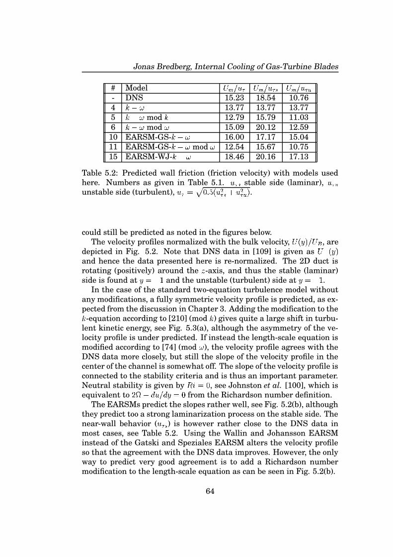
Jonas Bredberg, Internal Cooling of Gas-Turbine Blades
# Model�� � �
�� � �
� �� � �
� �
- DNS 15.23 18.54 10.764 �� � 13.77 13.77 13.775 �� � mod � 12.79 15.79 11.036 �� � mod � 15.09 20.12 12.5910 EARSM-GS- � � � 16.00 17.17 15.0411 EARSM-GS- � � � mod � 12.54 15.67 10.7515 EARSM-WJ- �� � 18.46 20.16 17.13
Table 5.2: Predicted wall friction (friction velocity) with models usedhere. Numbers as given in Table 5.1. �
� � stable side (laminar), � � �unstable side (turbulent), � � ��� �� � � � �� � � � �
� ��.
could still be predicted as noted in the figures below.The velocity profiles normalized with the bulk velocity,
� � � � � � � , aredepicted in Fig. 5.2. Note that DNS data in [109] is given as
� � � � �and hence the data presented here is re-normalized. The 2D duct isrotating (positively) around the � -axis, and thus the stable (laminar)side is found at � � � � and the unstable (turbulent) side at � � � � .
In the case of the standard two-equation turbulence model withoutany modifications, a fully symmetric velocity profile is predicted, as ex-pected from the discussion in Chapter 3. Adding the modification to the� -equation according to [210] (mod � ) gives quite a large shift in turbu-lent kinetic energy, see Fig. 5.3(a), although the asymmetry of the ve-locity profile is under predicted. If instead the length-scale equation ismodified according to [74] (mod � ), the velocity profile agrees with theDNS data more closely, but still the slope of the velocity profile in thecenter of the channel is somewhat off. The slope of the velocity profile isconnected to the stability criteria and is thus an important parameter.Neutral stability is given by ��� � , see Johnston et al. [100], which isequivalent to � � � � � � � � � from the Richardson number definition.
The EARSMs predict the slopes rather well, see Fig. 5.2(b), althoughthey predict too a strong laminarization process on the stable side. Thenear-wall behavior ( � � � ) is however rather close to the DNS data inmost cases, see Table 5.2. Using the Wallin and Johansson EARSMinstead of the Gatski and Speziales EARSM alters the velocity profileso that the agreement with the DNS data improves. However, the onlyway to predict very good agreement is to add a Richardson numbermodification to the length-scale equation as can be seen in Fig. 5.2(b).
64

Chap. 5: Results and Discussion
−1 −0.5 0 0.5 10
0.2
0.4
0.6
0.8
1
1.2
1.4
PSfrag replacements
� � � �
� � ������
mod�
�����mod
�
�����
DNS
(a)�����
models.
−1 −0.5 0 0.5 10
0.2
0.4
0.6
0.8
1
1.2
1.4
PSfrag replacements
� � � �
� � �EARSM-GS-
�����
EARSM-GS-�����
mod�
EARSM-WJ-�����
DNS
(b) EARSM models.
Figure 5.2: Velocity profiles, rotating 2D-duct
The velocity profile is the most important parameter in any enginee-ring flow and is of great value when discussing the turbulence models.Still in order to quantify turbulence models, a turbulent quantity is
65

Jonas Bredberg, Internal Cooling of Gas-Turbine Blades
necessary. In this case, the turbulent kinetic energy was chosen. Theturbulent kinetic energy profiles, normalized with the bulk velocity,� � � � � � �� , are shown in Fig. 5.3.
−1 −0.5 0 0.5 10
0.005
0.01
0.015
0.02
0.025
0.03
0.035
0.04
0.045
PSfrag replacements� � � ��
� � �
�����mod
������
mod�
�����
DNS
(a)�����
models.
−1 −0.5 0 0.5 10
0.005
0.01
0.015
0.02
0.025
PSfrag replacements� � � ��
� � �
EARSM-GS-�����
GS-�����
mod�
EARSM-WJ-�����
DNS
(b) EARSM models.
Figure 5.3: Turbulent kinetic energy, rotating 2D-duct
The first striking discrepancy is the terrible prediction of � using
66

Chap. 5: Results and Discussion
the modified � -equation in Fig. 5.3(a). Almost equally bad is the � -profile using the non-modified EVM, which, as for the velocity profile,is fully symmetric around the centerline of the duct. By adding thesimple Richardson number modification, the � -profile improves quite abit. The peaks in the turbulent kinetic energy close to the walls is fairlywell captured, as is the asymmetric profile. The overall agreement mayhowever leave a bit more to desire.
In the case of the EARSMs, Fig. 5.3(b), the EARSM-GS do not gre-atly change the symmetric profile of the standard EVM which can beexplained by the rather small anisotropy values captured by this mo-del. Since the model is constructed in such a way, that only small aniso-tropy values are allowed, it is expected that only a slightly asymmetri-cal profile of the turbulent kinetic energy is predicted. A comparisonof the EARSM-GS and the EARSM-WJ, shows some differences. TheEARSM-WJ is able to capture more of the re-laminarization processon the stable side, and the peak on the unstable side is a bit higher,although the differences are quite small. Similar to the two-equationmodel it is necessary to add the Richardson number modification tothe EARSMs to achieve satisfactory agreement with DNS data. FromFig 5.3, it is completely clear that the most important change is theRichardson number modification. Notable is also the small differencebetween the EARSM-GS- � � � mod � and � ��� mod � .
5.2 3D rib-roughened channel with perio-dic boundary conditions
The previous test case, the rotating smooth 2D duct, showed a signifi-cant impact of the chosen turbulence model on the predicted flowfield.It was concluded that the commonly used two-equation EVM did a poorjob for that case. Below it will be shown that the inclusion of ribs anda finite spanwise length reduces the importance of accurately captu-ring the rotational effects on the turbulence field. Secondary flows ge-nerated by geometry and system rotation are govern by pressure andCoriolis effects (in the momentum equations) – both which are exactlycaptured even by the simplest turbulence model. Through comparingan EARSM and an EVM it will be shown that the turbulence inducedsecondary flows (corner effects) and the rotational induced turbulenceare of significant lower magnitude and affect the result only margi-nally.
67

Jonas Bredberg, Internal Cooling of Gas-Turbine Blades
The geometric conditions for the present cases (pitch-to-height ratioof
� �� � � and a height-to-height ratio of � � � � �� � ) are shown in Fig.
5.4. As indicated in that figure, there are ribs on both walls, which arestaggered in relation to each other. For a staggered configuration, thecalculation domain is increased, as compared to a inline arrangement,because the symmetry condition on the centerline cannot be appliedand hence both the upper and lower walls with the ribs must be in-cluded in the computation. For the current case there exists howevera symmetry plane in the � -direction, at � � � � ���� , which enables thecalculation domain to be reduced to half. For these two cases (the sta-tionary and rotating), three different computation meshes have beenused: the coarse mesh which measured � � � � � � , the medium meshof � � � � � � � , and the fine mesh of � � � � � � � .
0
0.2
0.4
0.6
0.8
00.1
0.20.3
0.4
0
0.2
0.4
0.6
0.8
X
Y
Z
NU400380360340320300280260240220200180160140120100806040200
PSfrag replacements
�����
����
���
Figure 5.4: Streamlines and Nusselt number Abid et al. � � � model[3], stationary ribbed channel. Symmetry plane at � � � � ���� . Everysecond node is plotted.
In the licentiate thesis [19] an grid-independence check was inclu-ded. On the basis of the compared velocity profiles it was found suf-ficient to use only the coarse and medium meshes. For the presentanalysis computations made on the fine mesh was also included as it isapparent that near-wall sensitive quantities, such as the Nusselt num-
68
Chap. 5: Results and Discussion
ber shown in Fig. 5.5(a) is not grid-independent.The measured data of Iacovides et al. [86], [87] include: the streamwise
velocity,�
, the cross-stream velocity,�
, the shear stress � �� � , the nor-mal stresses, � � � � and � � , and the Nusselt number along the lowerwall1. The Reynolds number based on the channel height for both testcases is � � � � � 2, and the rotating number based on the channelheight for the rotating case is ��� � � � � . In the case of the velocityfield the data are taken from four selected points, at the top of the ribsand in between the ribs. These four points are defined by
� � � � (atthe inlet, centered on the first rib on the upper wall),
� � � � � � � (inthe middle between the first upper rib and the lower rib),
� � � � � �(at the top of the rib on the lower wall) and, finally, at
� � � � � � � (inthe middle between the rib on the lower wall and the second rib on theupper wall). The Nusselt number was measured along the lower wallexcluding the rib. The heat-flux is transmitted through an electricalheater fixed at both the upper and lower walls. This enables a con-stant heat-flux at the walls to be achieved, which is also the boundarycondition used in the computations.
The turbulence models used here are the Abid et al. � � � model andthe Gatski and Speziale EARSM [54] based on the Abid et al. � � �with the LRR pressure-strain model [120]. In the licentiate thesis [19]results using the SSG pressure-strain model in connection with theGatski and Speziale EARSM and the Chen and Patel zonal � ��� model[32] were also used.
The stationary and rotating cases are presented separately below,starting with the stationary case.
5.2.1 Stationary:The experimental and predicted Nusselt numbers with the two turbu-lence models for the stationary case are depicted in Fig. 5.5(b). Thepredicted Nusselt numbers are generally reasonable. The two turbu-lence models return similar profiles from
� � � � to the rib, althoughwith different levels. On the downstream side of the rib the modelsdeviate somewhat, with the ��� � predicting a larger plateau, indi-cating a larger secondary re-circulating zone downstream the rib. In[19] it was shown that the SSG-EARSM recovered slower than the twomodels presented here, more in agreement with the measurements.
1Heat transfer data was not measured for the rotating case.2The heat transfer data in [87] was however measured at ��� � ���� �����
69

Jonas Bredberg, Internal Cooling of Gas-Turbine Blades
0 0.2 0.4 0.6 0.8 10
50
100
150
200
250
300
350
400
450
500
PSfrag replacements
� �
� � �
FineMediumCoarseExp
(a) Different meshes.�����
model.
0 0.2 0.4 0.6 0.8 10
100
200
300
400
500
600
PSfrag replacements
� �
� � �EARSM�����
Exp
(b) Turbulence models.
Figure 5.5: Nusselt number. Stationary ribbed channel.
70
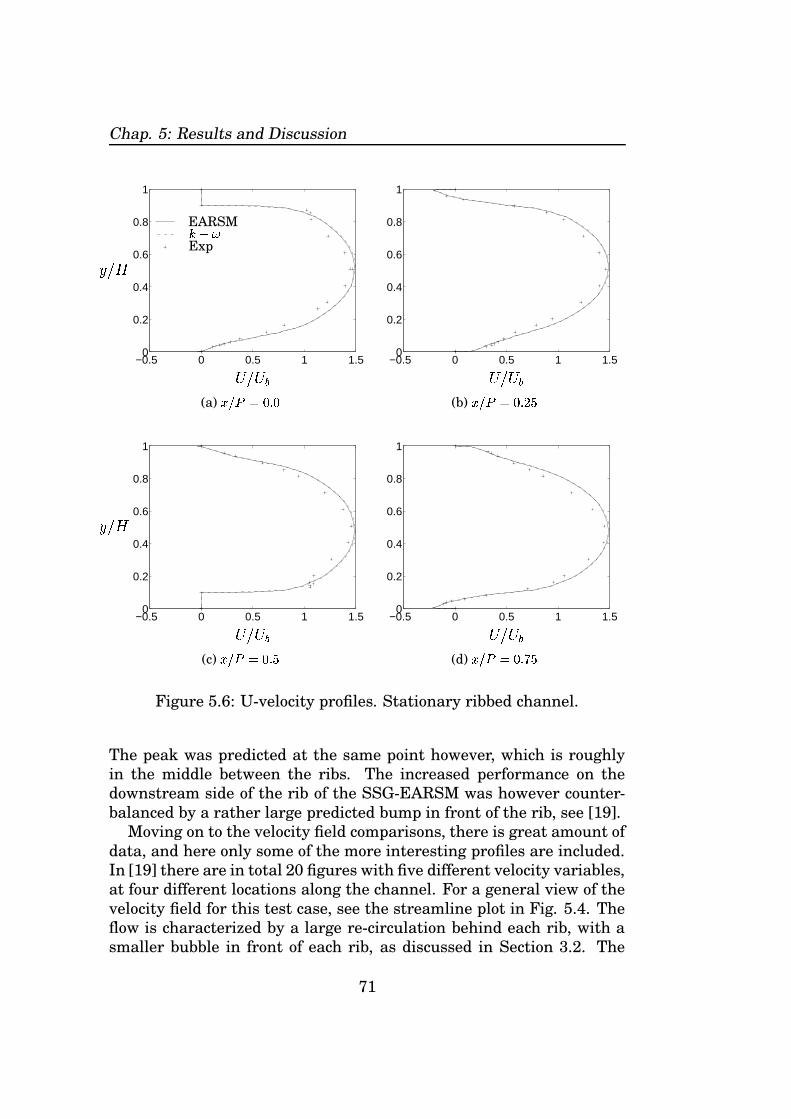
Chap. 5: Results and Discussion
−0.5 0 0.5 1 1.50
0.2
0.4
0.6
0.8
1
PSfrag replacements�����
� � ���
EARSM���Exp
(a) ��� � ��� �
−0.5 0 0.5 1 1.50
0.2
0.4
0.6
0.8
1
PSfrag replacements
� � ���(b) ��� � ��� ��
−0.5 0 0.5 1 1.50
0.2
0.4
0.6
0.8
1
PSfrag replacements
�����
� � ���(c) ��� � ���
−0.5 0 0.5 1 1.50
0.2
0.4
0.6
0.8
1
PSfrag replacements
� � ���(d) ��� � ��� ��
Figure 5.6: U-velocity profiles. Stationary ribbed channel.
The peak was predicted at the same point however, which is roughlyin the middle between the ribs. The increased performance on thedownstream side of the rib of the SSG-EARSM was however counter-balanced by a rather large predicted bump in front of the rib, see [19].
Moving on to the velocity field comparisons, there is great amount ofdata, and here only some of the more interesting profiles are included.In [19] there are in total 20 figures with five different velocity variables,at four different locations along the channel. For a general view of thevelocity field for this test case, see the streamline plot in Fig. 5.4. Theflow is characterized by a large re-circulation behind each rib, with asmaller bubble in front of each rib, as discussed in Section 3.2. The
71

Jonas Bredberg, Internal Cooling of Gas-Turbine Blades
−0.06 −0.04 −0.02 0 0.02 0.040
0.2
0.4
0.6
0.8
1
PSfrag replacements�����
������� � ����
EARSM� �Exp
(a) � � � � � �
−0.04 −0.02 0 0.02 0.04 0.060
0.2
0.4
0.6
0.8
1
PSfrag replacements
����� � ����(b) � � � � � ��
−0.04 −0.02 0 0.02 0.040
0.2
0.4
0.6
0.8
1
PSfrag replacements
�����
������� � � ��(c) ��� � ���
−0.06 −0.04 −0.02 0 0.02 0.040
0.2
0.4
0.6
0.8
1
PSfrag replacements
����� � � ��(d) ��� � ��� ��
Figure 5.7: � � � -shear stress. Stationary ribbed channel.
streamwise velocity profiles are plotted in Fig. 5.6, with an almostindistinguishable difference between the models, both being in fairlyclose agreement with the experiment data.
The shear stresses, � �� � , are depicted in Fig. 5.7. Both models returna rather good result for the important shear stress, which is the maininfluential Reynolds stress on the mean flow.
Fig. 5.8 shows the streamwise normal stress. As can be seen inthese figures, the EARSM achieve slightly better agreement with theexperimental data than the � ��� model, which is not surprising sinceEVMs cannot predict any anisotropy level for normal stresses.
The cross-stream normal stress, � � , included in [19] showed a rat-
72

Chap. 5: Results and Discussion
0 0.1 0.2 0.3 0.40
0.2
0.4
0.6
0.8
1
PSfrag replacements�����
� � � � � � ��
EARSM� ��Exp
(a) ��� � ��� �
0 0.1 0.2 0.3 0.40
0.2
0.4
0.6
0.8
1
PSfrag replacements
������ � � ��(b) ��� � ��� ��
0 0.1 0.2 0.3 0.40
0.2
0.4
0.6
0.8
1
PSfrag replacements
�����
������ � � ��(c) ��� � ���
0 0.1 0.2 0.3 0.40
0.2
0.4
0.6
0.8
1
PSfrag replacements
������ � � ��(d) ��� � ��� ��
Figure 5.8: � � � � -normal stress. Stationary ribbed channel.
her poor presentation of the SSG-EARSM, where the �� � fluctuatesviolently behind the ribs, resulting in slow convergence rates. The con-clusion was that the reason for this behavior was most likely mesh-dependent. The SSG-EARSM was not included here because of this,although the current mesh ( � � � � � � � ) is most probably better thanthe one used in [19].
5.2.2 Rotating:For the rotating case, there are two sets of measurement data: velocitydata for either a positive rotation at ����� � �� � or a negative rotation
73
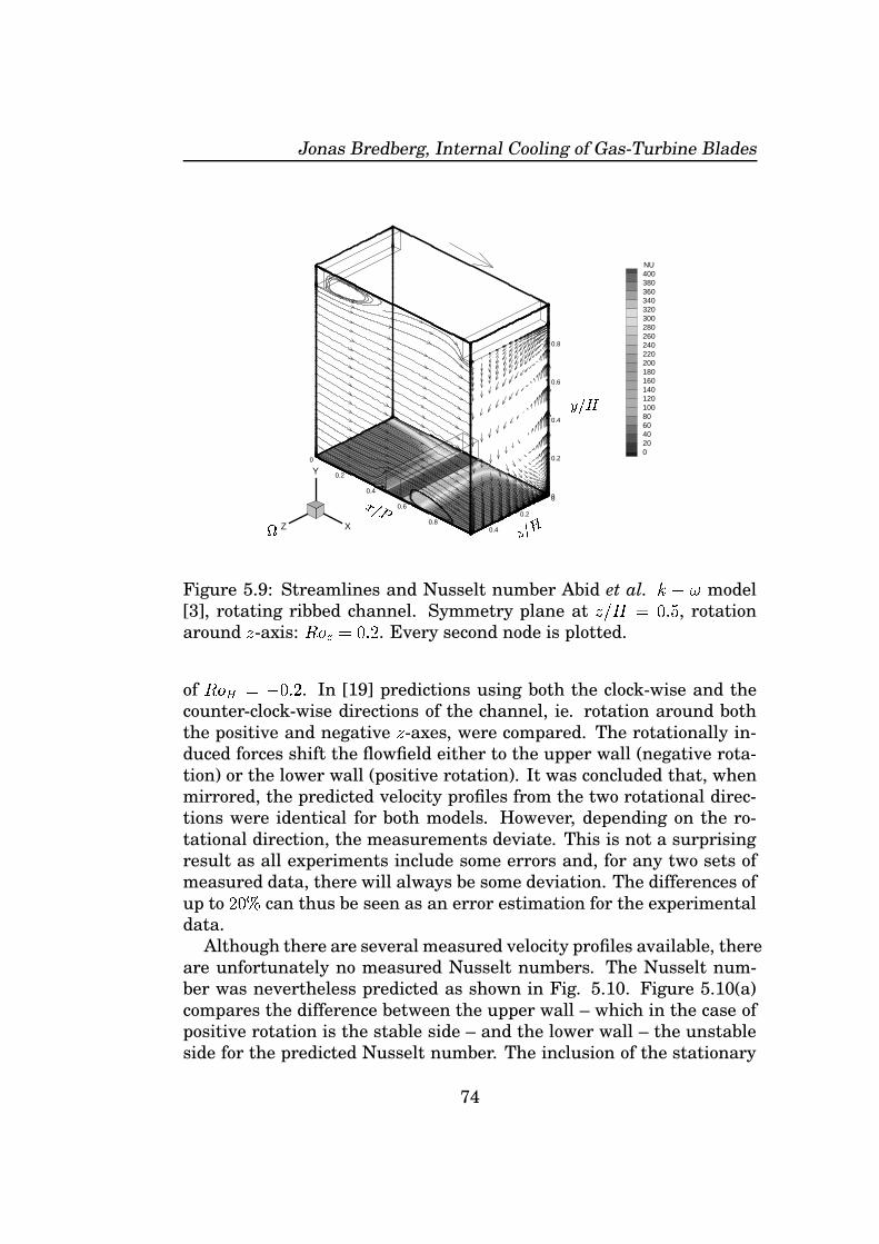
Jonas Bredberg, Internal Cooling of Gas-Turbine Blades
0
0.2
0.4
0.6
0.8
0
0.2
0.4
0
0.2
0.4
0.6
0.8
X
Y
Z
NU400380360340320300280260240220200180160140120100806040200
PSfrag replacements
�����
����
����
Figure 5.9: Streamlines and Nusselt number Abid et al. � � � model[3], rotating ribbed channel. Symmetry plane at � ��� � �� � , rotationaround � -axis: ��� � �� �� � . Every second node is plotted.
of ��� � � � � � . In [19] predictions using both the clock-wise and thecounter-clock-wise directions of the channel, ie. rotation around boththe positive and negative � -axes, were compared. The rotationally in-duced forces shift the flowfield either to the upper wall (negative rota-tion) or the lower wall (positive rotation). It was concluded that, whenmirrored, the predicted velocity profiles from the two rotational direc-tions were identical for both models. However, depending on the ro-tational direction, the measurements deviate. This is not a surprisingresult as all experiments include some errors and, for any two sets ofmeasured data, there will always be some deviation. The differences ofup to � � can thus be seen as an error estimation for the experimentaldata.
Although there are several measured velocity profiles available, thereare unfortunately no measured Nusselt numbers. The Nusselt num-ber was nevertheless predicted as shown in Fig. 5.10. Figure 5.10(a)compares the difference between the upper wall – which in the case ofpositive rotation is the stable side – and the lower wall – the unstableside for the predicted Nusselt number. The inclusion of the stationary
74

Chap. 5: Results and Discussion
0 0.2 0.4 0.6 0.8 10
100
200
300
400
500
600
PSfrag replacements
� �
� � �StationaryRot-lowerRot-upperStat-exp.
(a) Stationary vs rotating.�����
model.
0 0.2 0.4 0.6 0.8 10
100
200
300
400
500
600
700
PSfrag replacements
� �
� � �EARSM�����
Exp
(b) Turbulence models.
Figure 5.10: Nusselt number. Rotating ribbed channel.
75

Jonas Bredberg, Internal Cooling of Gas-Turbine Blades
data gives a visual impression of the effect of rotation.The main difference between the predicted Nusselt number for the
rotating case as compared with the stationary case is the shift of theNusselt number on the lower wall (increased) and upper wall (decrea-sed), as can be seen in Fig. 5.10(a). The decrease on the upper wall isvery slight, less than 10%. On the lower wall the increase is howevermuch more dominant and amounts to roughly 30%, which is surely adesired affect. From this it can be concluded that the rotation increa-ses the general level of heat transfer in ribbed channels. The relativechange of the heat transfer is of course associated with the increasein turbulent kinetic energy on the unstable side (lower) and a simi-lar decrease in the turbulent kinetic energy on the stable side (upper).Through the heat transfer model used in this report, equation Eq. 2.23,the eddy viscosity is directly related to the heat transfer, and thus anincrease in turbulent kinetic energy would yield a higher Nusselt num-ber and vice versa.
Apart from the change in the magnitude of the Nusselt number, theprofiles are essentially the same, and the same conclusion as was madefor the stationary case can be drawn regarding the performance in frontof the rib and behind the rib. It can thus be concluded that there is nosignificant advantage of using an EARSM compared to an EVM for arib-roughened 3D duct, stationary or rotating. A correct level of Nus-selt number was also predicted for this case in Paper VII [25] using a� � � turbulence model.
Moving on to the velocity field, the streamlines for the Abid et al. tur-bulence model are shown in Fig. 5.9. Comparing the rotating case, Fig.5.9, with the stationary case, Fig. 5.4, reveal a change in flow structure.The latter, stationary case, has a symmetric behavior, where the flow-fields on the upper wall and the lower wall are essential the same,although shifted half a pitch. The rotating case, on the other hand,do not posses this symmetry, as the Coriolis force ( � � � �
) shifts the ve-locity field downwards. Consequently the re-circulation region behindthe upper first rib is much larger than that behind the lower mid-rib,see Fig. 5.11. As in the stationary case, there is a re-circulation bubblein front of the ribs as well, although this is very much suppressed onthe lower wall, while it is amplified on the upper wall.
The streamwise velocity profiles are depicted in Fig. 5.11. Thedescribed differences in the re-attachment point behind the upper andlower rib is shown in this figure, although it is perhaps graphicallymore clear in the streamline plot of Fig. 5.9. In Fig. 5.11(b) and5.11(c) it can be seen that the flow is still moving backwards along
76

Chap. 5: Results and Discussion
−0.5 0 0.5 1 1.50
0.2
0.4
0.6
0.8
1
PSfrag replacements�����
� � ���
EARSM���Exp
(a) ��� � ��� �
−0.5 0 0.5 1 1.50
0.2
0.4
0.6
0.8
1
PSfrag replacements
� � ���(b) ��� � ��� ��
−0.5 0 0.5 1 1.50
0.2
0.4
0.6
0.8
1
PSfrag replacements
�����
� � ���(c) ��� � ���
−0.5 0 0.5 1 1.50
0.2
0.4
0.6
0.8
1
PSfrag replacements
� � ���(d) ��� � ��� ��
Figure 5.11: U-velocity profiles. Rotating ribbed channel.
the upper wall five step heights downstream of the upper rib (Fig.5.11(c)). Along the lower wall, however, the flow is attached five stepheights downstream of the rib (Fig. 5.11(a)). In Fig. 5.11(d), it can beseen that, despite the downward shift of the flowfield, the flow still re-attaches along the upper wall and thus the pitch in this ribbed channelis sufficiently large to enable increased heat transfer – through hig-her turbulence levels – even in the rotating case. The downward shiftof the flow also affect the smaller re-circulation bubbles upstream theribs. Comparing the velocity profiles upstream the upper and lowerribs, Figs 5.11(b) and 5.11(d), it is evident that the near-wall velocityis much higher 2.5 step heights upstream of the lower rib than at the
77

Jonas Bredberg, Internal Cooling of Gas-Turbine Blades
−0.1 −0.05 0 0.050
0.2
0.4
0.6
0.8
1
x
PSfrag replacements�����
EARSM� ��Exp
(a) � � � � � �
−0.1 −0.05 0 0.050
0.2
0.4
0.6
0.8
1
PSfrag replacements
����� � ����(b) � � � � � ��
−0.05 0 0.050
0.2
0.4
0.6
0.8
1
PSfrag replacements
�����
������� � � ��(c) ��� � ���
−0.05 0 0.050
0.2
0.4
0.6
0.8
1
PSfrag replacements
����� � � ��(d) ��� � ��� ��
Figure 5.12: � � � -shear stress. Rotating ribbed channel
same distance upstream of the upper rib, indicating a much strongerupstream re-circulating bubble on the upper wall. An effect which isdifficult to discern from the predicted Nusselt numbers in Fig. 5.10(a).
Both models predict the downward shift of the velocity field, dueto rotation, accurately, with a maximum velocity around � ��� � �� � ,slightly changing from one part of the channel to another owing to thealternating blockage effect of the ribs. The overall behavior of the twomodels is satisfying, with only a marginal effect of the additional termsin the EARSM formulation.
The shear stress, � � � , is shown in Fig. 5.12. The agreement betweenthe predictions and the measurements have deteriorated as compared
78

Chap. 5: Results and Discussion
0 0.1 0.2 0.3 0.4 0.50
0.2
0.4
0.6
0.8
1
PSfrag replacements�����
� � � � � � ��
EARSM���Exp
(a) ��� � ��� �
0 0.1 0.2 0.3 0.40
0.2
0.4
0.6
0.8
1
PSfrag replacements
������ � � ��(b) ��� � ��� ��
0 0.1 0.2 0.3 0.4 0.50
0.2
0.4
0.6
0.8
1
PSfrag replacements
�����
������ � � ��(c) ��� � ���
0 0.1 0.2 0.3 0.4 0.50
0.2
0.4
0.6
0.8
1
PSfrag replacements
������ � � ��(d) ��� � ��� ��
Figure 5.13: � � � � -normal stress. Rotating ribbed channel.
with the stationary case, see Fig. 5.7, and there is also a larger diffe-rence between the two turbulence models. The most notable problema-tic area is at the top of the lower rib, in Fig. 5.12(c), where none of themodels capture neither the correct profile nor the correct level. Movingfurther up in the channel at this position, the experiment shows almosta linear relation of the shear stress between the lower and upper wall,which none of the models capture. The deviation is larger for the EVM,although the profiles of the EARSM act rather strangely – in the centerpart of the channel, the EARSM predicts zero shear stress, which is notfound in the measurements.
Figure 5.13 shows the normal stress. As for the stationary case, the
79

Jonas Bredberg, Internal Cooling of Gas-Turbine Blades
EARSM return slightly better agreement, which reflects the increasedphysics involved in these models, enabling the models to deviate fromthe isotropic relation of the Boussinesq hypothesis.
80
Chapter 6
Summary of Papers
Below are some comments on the papers included in thisthesis. They are here to place the papers in a broader frameof reference and also to connect them more closely with themain objectives of the present research. The summaries areintentionally different from the abstracts included in the pa-pers, and are made to emphasize useful insights not fullyrecognized at the time. Furthermore, in contrast to the ab-stracts, these summaries are not deprived of healthy criti-cism which have been valuable for the progress of this work.
6.1 Paper IJ. Bredberg and L. Davidson”Prediction of flow and heat transfer in a stationary two-dimensionalrib roughened passage using low-Re turbulent models”In Proceedings of 3:rd European Conference on Turbomachinery: FluidDynamics and Thermodynamics, pages 963-972, IMechE 1999.
The paper presents a comparison between four different turbulencemodels on a 2D rib-roughened channel. Complementary to the evalu-ation of the turbulence models, the paper validates numerical proce-dures implemented in CALC-BFC, namely the periodic boundary con-ditions and the blockage routines. As a result of this, a disproptio-nally large part of the paper is devoted to numerics. Being the firstproper paper, excluding the contribution to the ERCOFTAC workshop[22], the structure and presentation of the results is slightly differentto forthcoming papers. Nevertheless the conclusions from this paper
81

Jonas Bredberg, Internal Cooling of Gas-Turbine Blades
constitutes the foundation for later work. Apart from the thesis forthe degree of licentiate [19] written at the same time as this paper, theEARSM type of turbulence models were not to be used anymore, as aresult of the findings in this paper. The grid dependency analysis sho-wed that the criteria of Wilcox [209] for the � boundary condition istoo strong. In subsequently simulations ��� was to be specified only forthe two first interior grid-nodes. The paper concluded that none of theevaluated turbulence models were adequate for heat transfer predic-tion. Models which performed reasonable in the � � � � � � case, didpoorly in the � � � � � � case and vice versa. This erroneous Reynoldsnumber dependency for heat transfer using eddy-viscosity models wasto be further discussed in the next paper. This paper also visualizethe difficulties in specifying the correct boundary condition, as some ofthe large discrepancies in the predicted Nusselt number around the ribfor the � � � � � � case can be attributed to the simplistic treatmentof wall heat flux at the rib-faces. Although the code was later modi-fied to enable conjugate heat transfer problems to be solved effectively,discrepancies still persisted in this area.
6.2 Paper IIJ. Bredberg, L. Davidson and H. Iacovides”Comparison of Near-wall Behavior and its Effect on Heat Transfer for� � � and ���� Turbulence Models in Rib-roughened 2D Channels”In Proceedings of 3:rd Int. Symposium on Turbulence, Heat and MassTransfer, pages 381-388, eds. Y. Nagano and K. Hanjalic and T. Tsuji,Aichi Shuppan 2000.
The paper is the result of questions raised in the previous paper anda fruitful visit to Prof. Launders group at UMIST, Manchester. Theco-author Dr. Iacovides is part of that group which has a long traditionon numerical simulations on configurations of interest for this thesis,as the one in question for this paper. The measured data for the si-mulations was also the result of a diploma work at UMIST [144]. Dr.Iacovides greatfully supplied the data and gave valuable discussionsand suggested important alterations to the paper. The main emphasisof the paper was to discuss and try to explain the believed erroneousReynolds number dependencies of eddy-viscosity models for heat trans-fer predictions in separated flows. The results from the previous papercould only suspect such an idea, as the two studied cases different both
82

Chap. 6: Summary of Papers
in Reynolds number as well as in geometry. The advantage of usingthe UMIST-data, which only varied in Reynolds number, for such ananalysis is obvious. In addition to the zonal �� � and the ���� model,studied previously, the Launder-Sharma � � � [121] was also includedin this paper. In retrospective the used ��� � model [3] should havebeen substituted with the more commonly employed model by Wilcox[207], to make the results in the paper attractive to a broader audi-ence. The conclusions are however general, and confirms the suspicionraised: two-equation turbulence models gives a too strong Reynoldsdependency for heat transfer in separated flows. The importance ofcorrectly estimating the near-wall turbulence level when employing aconstant Prandtl number heat transfer model for an accurate predic-tion of Nusselt number was shown. Although the lack of turbulencemeasured data, the noted strong connection between heat transfer andturbulence has later been verified repeatedly. Extending the analysisto the solved turbulent quantities in the latter part of the paper wasless conclusive. The importance of a correctly estimated length-scalein separated regions was however addressed. The result for the turbu-lent kinetic energy ( � ) showed a distinct difference between the � ���model and the other two models, which confirms the futility of trying torelate heat transfer to only one of the solved turbulent quantities. Theinaccuracy of the zonal model, for which the length-scale is only vagu-ely effected by the flow, is a testimony of this. The paper could howevernot give any conclusive solution to the erroneous Reynolds number de-pendency, and it is unfortunate that the effect of the Yap correctionfor the ��� � model was not included, as that could have given valu-able information for further research. The Yap-correction thread wasagain given attention in Paper VI, however without any decisive con-clusion. Paper II also included the predicted friction coefficient alongthe lower, rib-roughened, wall for both Reynolds number. The compa-rison of
" �and
� � re-confirms the erroneous behaviour of employingReynolds analogy when estimating heat transfer in separated flows.The
" �-plots also resulted in the final abolishment of zonal models, as
this type of models was found to be inadequate for estimating even theflowfield in separated flows.
6.3 Paper IIIJ. Bredberg, S.-H. Peng and L. Davidson”On the Wall Boundary Condition for Computing Turbulent Heat Trans-
83

Jonas Bredberg, Internal Cooling of Gas-Turbine Blades
fer with �� � Models”In Proceedings of the ASME Heat Transfer Division - 2000, HTD-Vol.366-5, pages 243-250, ed. J.H. Kim, ASME 2000.
In accordance with the obligations made to GTC, Paper III repre-sents the first attempt to develop a method to estimate heat trans-fer rates sufficiently accurate using only modest computation require-ments. The final goal of the project is to simulate the flow and heattransfer inside a turbine blade. Previous achievements in the litera-ture with numerical simulations indicates the necessity of fully resol-ving the geometry of the serpentine ducts, including the ribs. A roughestimation of the amount of computational nodes for a typical 3D geo-metry however showed the impossibility of making a LRN simulation.Thus it would be necessary to employ wall function based turbulencemodels. On the basis of results from computations performed on 3Drib-roughened channels the prospect of achieving a high degree of fi-delity using such an approach is however small. Time was spent tofind a model and/or method with a higher ratio of accuracy to compu-tational efforts. The literature survey gave however only a few alter-natives to the standard wall function model. The study, which laterresulted in Paper IV, showed the improvement through solving, ratherthan setting, the turbulent kinetic energy equation, as is done in theLaunder-Spalding (LS) model. The Chieng-Launder (CL) model, whichsub-divides the first cell into layers, each with its own individual treat-ment was also studied. Although the latter model only yields meagerimprovements compared to the LS model, the idea of splitting the firstcell into a viscous and a turbulent region with its respectively model-ling approach was adopted in the present paper. The stability problemsencountered by the author using the CL model however necessitated achange in methodology. It was early decided to base the new modelon a ��� � model rather than a � � � as in the Chieng-Launder mo-del, mainly due to the previous good experience – within the group– when using the Wilcox models. Furthermore an additional coeffici-ent was introduced to enhance numerical stability through blendingthe two layers, rather than adding them together. The latter approachalso substantially facilitated the treatment within both the LRN andHRN zones, and enabled an almost straight-forward adoption of wellestablished methods for the respective zones. The resulting model ho-wever became sensitive to the blending function which can be noted inthe peculiar profiles for the Nusselt number on intermediate refinedmeshes. Improved results could only be achieved using a non-standard
84

Chap. 6: Summary of Papers
heat transfer model, which is seen as a drawback of the model. Alt-hough the model give results similar in accuracy to those using theWilcox � � � model on refined meshes and to those using the LS-modelon coarser meshes, a general high degree of accuracy was not achieved.However as most experiences in life, new ideas need to mature beforethey can be employed successfully. The knowledge gained with thismodel later resulted in the model with a substantially improved heattransfer performance as shown in Paper VII and VIII.
6.4 Paper IVJ. Bredberg”On the Wall Boundary Condition for Turbulence Models”Report 00/4, Department of Thermo and Fluid Dynamics, ChalmersUniversity of Technology, 2000
This paper is the result of the study on wall functions along the deve-lopment of the hybrid model in Paper III. The paper is mainly devotedto the HRN type of turbulence models and special treatments neededto take care of the large variation in the buffer layer. Paper V is enti-rely focused on the LRN turbulence model and the aspect of accuratelymodelling the viscous sub-layer. The present paper concerns, with afew exceptions, on ��� � models and should be seen as an extensionto Paper III, rather than a general overview on wall treatments. Thethorough derivations and explanations to modelling approaches madefor Paper III may also be useful as an introduction to constructing newwall functions. In addition the paper give complementary informationfor the description of the Launder-Spalding and Chieng-Launder mo-dels. The presentation of alternatives to the standard wall function forthe temperature equation may also be valuable.
6.5 Paper VJ. Bredberg”On Two-equation Eddy-Viscosity Models”Report 01/8, Department of Thermo and Fluid Dynamics, ChalmersUniversity of Technology, 2001.
Paper V constitutes a comprehensive work on theory and modelling
85

Jonas Bredberg, Internal Cooling of Gas-Turbine Blades
approaches made for two-equation turbulence models. Similar to PaperIV, this internal report is a also the product of research made in con-nection with another published paper. For the development of the � � �model in Paper VI it was necessary to thoroughly examine the conceptsand relations of the secondary quantity, ie. � , � and � in two-equationEVMs. Most of the latter part of the report, excluding the appendices,also focus on similarities and differences between a � ��� and a � � �model. The report tries to explain, especially in Chapter 6 and 7, theideas behind modelling approaches made for turbulence models. Theattempt however falls short of the target, mainly due to the, in manycases, lacking theoretical foundations for terms and functions introdu-ced in turbulence models. The report is divided into several separatedsections, for which the introduction part is treated in Chapter 1 and2. Chapter 3 deals with ’exact’ relations, from derived equations andDNS-data. The modelling approaches made for EVMs are treated eit-her in Chapter 4 or 5. The partition is made dependent on whetherthe models are based on what is referred to as the classic theory, ie.mainly on experimental data, or based on data from numerical simu-lations (DNSs). As stated above the latter part of the report (Chapter6 and 7) compares and summarizes modelling approaches for the dif-ferent types of two-equation models. A particular important additionis appendices A and B which give a complete list of eleven turbulencemodel with comments (A) together with their usefulness in three diffe-rent generalized test-cases (B). Other useful information is given in eg.Section 4.1.2 where different types of wall distance relation are given.From a modelling point of view Sections 6.3, 6.4, 7.3 and 7.4 along withAppendix C are of interest as these sections attempts to explain therationale behind the introduced cross-diffusion terms in the new � � �model. These parts could be treated as an addition to Paper VI.
6.6 Paper VIJ. Bredberg, S.-H. Peng and L. Davidson”An improved � ��� turbulence model applied to recirculating flows”Accepted for publication in Int. J. Heat and Fluid Flow, 2002.
The initiation to this paper is a combination of several factors. Thestrive to improve upon the previous revealed inadequacy of many EVMsis the dominant factor. Paper I and II showed the erroneous Reynoldsnumber dependency for heat transfer predictions that two-equation
86
Chap. 6: Summary of Papers
turbulence model experience. It should however be admitted that themodel presented in Paper VI does not improve upon this deficiency.Another important contribution is the previously developed a cross-diffusion modified � � � turbulence model [162], which has showed tohave some advantages feature compared to the standard � � � model.That model was unfortunately optimized using incorrect DNS-data, re-sulting in insufficient accuracy for fully developed channel flow. A re-medy to this, with maintained accuracy for other flows, is given by thenew model. Although the predictability on coarse mesh is only treatedin Paper VIII, the present model was developed with grid-robustnessin mind. It is considered that much of the grid sensitivity experiencedusing LRN turbulence model arise from too stiff damping functions. Asa result, the degree of empiricism added to the new model was main-tained at a minimum. It was possible through the introduction of aviscous cross-diffusion term in the � -equation to reduce the number ofdamping functions to only one. An additional advantage with this termis that the wall boundary condition for � could be made theoreticallyconsistent with DNS-data. Furthermore the cross-diffusion terms re-duces the sensitivity to the specification of � � for free shear flows, ascompared with other ��� � models. The inclusion of free shear flowswas the result of a reviewer comments (which is greatfully acknowled-ged), and not considered in the designing of the model. It should berecognized that there is always a certain degree of freedom in the spe-cifications of coefficients and terms in the transport equations. For thepresent model these numerical optimizations were made in as close ac-cordance as possible with well accepted rules and values. Thus many ofthe coefficients in this model are equivalent to those used in the stan-dard � ��� model, eg.
"� � � � ��� � � � � "�� � � ����� � "�� � � ��� � . A number
of different values were tried for� � , the one used (=1.8) is slightly un-
conventional, but it offered the best compromise. As a defense one maynote that Wilcox �� � models use the even more extreme value
� � � � .It was also noted that a change in the cross-diffusion term coefficient(" � ) would enable a more common value, however at the expense of a
change in the boundary condition for � from its theoretically exact va-lue. The discussion in Paper V, Section 7.3, should also be considered:“there is little theoretical foundation for any particular value on
� � asthe Schmidt numbers should generally vary as a function of the walldistance”.
87
Jonas Bredberg, Internal Cooling of Gas-Turbine Blades
6.7 Paper VIIJ. Bredberg and L. Davidson”Prediction of turbulent heat transfer in stationary and rotating U-ducts with rib roughened walls”Accepted to the 5:th International Symposium on Engineering Turbu-lence Modelling and Measurements, 2002.
Paper VII and Paper VIII were written simultaneously with this in-troduction part of the thesis and hence the comments made here couldas well have been included in the papers. The papers may be conside-red inconsequently numbered, as this paper (VII) presents the results,while the next (VIII) discusses the model. The papers were howeverwritten in this order. There is a small addition to the turbulence modelin Paper VII as compared to Paper VIII. This is the limiters which areincluded in Eq. 6. These are the result of stability problems encounte-red when using too a coarse mesh to approximate the gradients in thecross-diffusion terms. Their inclusion is however not controversial, asthey are in accordance with physics. The limitation of the viscous termensures that it is only affecting the flow in the near-wall region wherethe gradients of � and � are of opposite sign. The limit for the turbulentterm is also theoretically well posed. The only ambiguity is the dam-ping function in the turbulent term, as the heat transfer prediction issensitive to the exact formulation of this function. The term could ho-wever not be removed as this would change the predicted result evenfor simple channel flow. Although these comments, the results presen-ted in the paper represent a good combination of accuracy and compu-tational efficiency. There is only a small flaw with the used mesh whichresults in unphysical variation of the Nusselt immediate upstream theribs, mostly notable in Fig. 5 and 6.
6.8 Paper VIIIJ. Bredberg and L. Davidson”Low-Reynolds Number Turbulence Models: An Approach for ReducingMesh Sensitivity”Submitted for journal publication.
When initiating, in Paper III, the development of a turbulence mo-del that would be capable of accurate near-wall prediction on coarser
88
Chap. 6: Summary of Papers
meshes, the author was only familiar with the work made by Grotjansand Menter [60]. Later, as noted by the introduction, there have beenan increased interest in such models, especially at UMIST. It shouldbe noted that even though academia have used LRN turbulence mo-dels as a basis when performing numerical simulation for a long timenow [101], [121], industry have strongly relied on wall function ba-sed methods, and only recently started to experimenting with modelsrequiring more refined meshes. The contribution of Paper VIII, is thussimilarly to Paper III, aimed at constructing reliable engineering mo-dels rather than achieving unmatched accuracy. Mating the previouslydeveloped � ��� model (Paper VI) with some simple correction derivedfrom experience gained with the hybrid model (Paper III) resulted ina very trustworthy model, applicable for meshes with the first near-wall node at � � � � . The decrease in mesh demands may be considermarginal, however as notable in eg. Fig. 9 and Table 3 the accuracycould be maintained using only one-tenth of the number of nodes (fora 3D application). Comparing also the minor modification necessaryto the baseline model, with the additional performance gain, it is con-sidered as a well invested work. Contrary to the hybrid model (PaperIII) modifications are not needed for any other wall boundary condi-tions, apart from the one used in the turbulence model. The increasedstability via the extension presented in Paper VII, is recommended forcomplex geometries. It would be desirable to continue this work to furt-her extend the applicability of the model to include computation madeon meshes for which the first node is located within the buffer layer,��� � � � � . Such a model may however necessitate modificationsto both the momentum and temperature equations in addition to theturbulence equations.
89

Jonas Bredberg, Internal Cooling of Gas-Turbine Blades
90
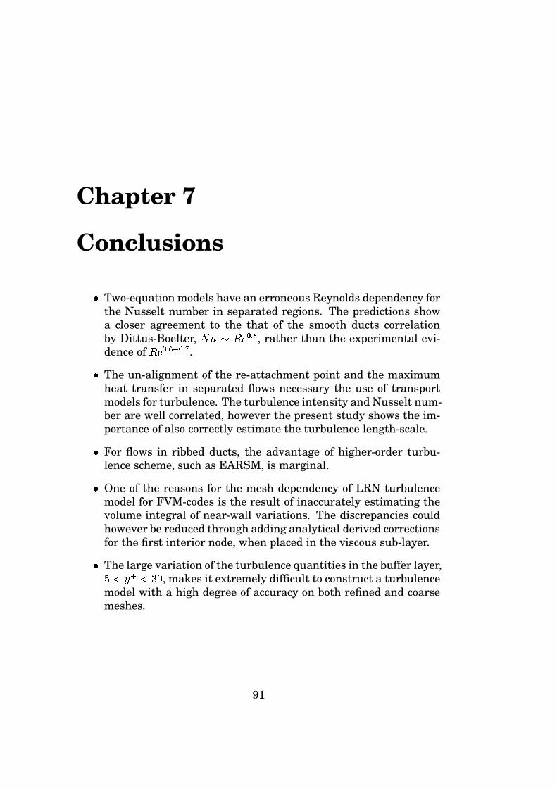
Chapter 7
Conclusions
� Two-equation models have an erroneous Reynolds dependency forthe Nusselt number in separated regions. The predictions showa closer agreement to the that of the smooth ducts correlationby Dittus-Boelter,
� � � � �� �, rather than the experimental evi-
dence of � �� � � �
.� The un-alignment of the re-attachment point and the maximum
heat transfer in separated flows necessary the use of transportmodels for turbulence. The turbulence intensity and Nusselt num-ber are well correlated, however the present study shows the im-portance of also correctly estimate the turbulence length-scale.
� For flows in ribbed ducts, the advantage of higher-order turbu-lence scheme, such as EARSM, is marginal.
� One of the reasons for the mesh dependency of LRN turbulencemodel for FVM-codes is the result of inaccurately estimating thevolume integral of near-wall variations. The discrepancies couldhowever be reduced through adding analytical derived correctionsfor the first interior node, when placed in the viscous sub-layer.
� The large variation of the turbulence quantities in the buffer layer,� � � � � � , makes it extremely difficult to construct a turbulencemodel with a high degree of accuracy on both refined and coarsemeshes.
91

Jonas Bredberg, Internal Cooling of Gas-Turbine Blades
92
Bibliography
[1] A. Abdon and B. Sunden. A numerical study on the influence ofrib shape on the thermodynamic performance of a cooling duct.In Proceedings of the ASME IMECE 2001. The American Societyof Mechanical Engineers, 2001.
[2] K. Abe, T. Kondoh, and Y. Nagano. A new turbulence model forpredicting fluid flow and heat transfer in separating and reat-taching flows - I. flow field calculations. Int. J. Heat and MassTransfer, 37:139–151, 1994.
[3] R. Abid, C. Rumsey, and T. Gatski. Prediction of nonequilibriumturbulent flows with explicit algebraic stress models. AIAA Jour-nal, 33:2026–2031, 1995.
[4] S. Acharya, S. Dutta, and T.A. Myrum. Heat transfer in turbu-lent flow past a surface-mounted two-dimensional rib. J. HeatTransfer, 120:724–734, 1998.
[5] S. Acharya, S. Dutta, T.A. Myrum, and R.S. Baker. Periodicallydeveloped flow and heat transfer in a ribbed duct. Int. J. Heatand Mass Transfer, 36:2069–2082, 1993.
[6] S. Acharya, S. Dutta, T.A. Myrum, and R.S. Baker. Turbulentflow past a surface mounted two-dimensional rib. J. Fluids Engi-neering, 116:238–246, 1994.
[7] R.S. Amano. Development of a turbulence near-wall model andits application to separated and reattached flows. NumericalHeat Transfer, 7:59–75, 1984.
[8] R.S. Amano, M.K. Jensen, and P. Goel. A numerical and expe-rimental investigation of turbulent heat transport downstreamfrom an abrupt pipe expansion. J. Heat Transfer, 105:862–869,1983.
93

Jonas Bredberg, Internal Cooling of Gas-Turbine Blades
[9] J. Antoniou and G. Bergeles. Development of the reattached flowbehind surface-mounted two-dimensional prisms. J. Fluids Engi-neering, 110:127–1336, 1988.
[10] J. Bardina, J.H. Ferziger, and R.S. Rogallo. Effect of rotationon isotropic turbulence: computation and modelling. J. FluidMechanics, 154:321–336, 1985.
[11] W. Bauer, O. Haag, and D.K. Hennecke. Accuracy and robustnessof nonlinear eddy viscosity models. Int. J. Heat and Fluid Flow,21:312–319, 2000.
[12] J.W. Baughn and X. Yan. Local heat transfer measurements insquare ducts with transverse ribs. In National Heat TransferConference, 1992.
[13] D.L. Besserman and S. Tanrikut. Comparison of heat transfermeasurements with computations for turbulent flow around 180deg bend. J. Turbomachinery, 114:865–871, 1992.
[14] B. Bonhoff, T. Schneider, B. Johnson, and I. Jennions. Predictionfor turbulent flow in rotating and non rotating coolant channels.In 2:nd Int. Symp. on Turbulence, Heat and Mass Transfer, 1997.
[15] B. Bonhoff, U. Tomm, B.V. Johnson, and I. Jennions. Heattransfer predictions for rotating u-shaped coolant channels withskewed ribs and with smooth walls. In Int. Gas Turbine & Aero-engine Congress and Exhibition, 1997.
[16] J.P. Bons and J.L. Kerrebrock. Complementary velocity andheat transfer measurements in a rotating cooling passage withsmooth walls. J. Turbomachinery, 121:651–662, 1999.
[17] T.V. Boussinesq. Mem. pres Acad. Sci.,3rd ed Paris XXIII p. 46,1877.
[18] P. Bradshaw. The analogy between streamline curvature andbuoyancy in turbulent shear flow. J. Fluid Mechanics, 36:177–191, 1969.
[19] J. Bredberg. Prediction of flow and heat transfer inside turbineblades using EARSM, � � � and � � � turbulence models. Thesisfor the Degree of Licentiate of Engineering, Dept. of Thermo andFluid Dynamics, Chalmers University of Technology, Gothen-burg, 1999. Also available at www.tfd.chalmers.se/˜bredberg.
94

BIBLIOGRAPHY
[20] J. Bredberg. On the wall boundary condition for turbulence mo-del. Report 00/4, Dept. of Thermo and Fluid Dynamics, ChalmersUniversity of Technology, Gothenburg, 2000. Also available atwww.tfd.chalmers.se/˜bredberg.
[21] J. Bredberg. On two-equation eddy-viscosity models. Report01/8, Dept. of Thermo and Fluid Dynamics, Chalmers Uni-versity of Technology, Gothenburg, 2001. Also available atwww.tfd.chalmers.se/˜bredberg.
[22] J. Bredberg and L. Davidson. Case 7.2: Two-dimensional flowand heat transfer over a smooth wall roughened with squaredribs. In 7th ERCOFTAC/IAHR workshop on refined turbulencemodeling, Manchester, 1998.
[23] J. Bredberg and L. Davidson. Prediction of flow and heat trans-fer in a stationary 2-D rib roughened passage using low-Re tur-bulent models. In 3:rd European Conference on Turbomachinery,pages 963–972, London, 1999. IMechE.
[24] J. Bredberg and L. Davidson. Low-Reynolds number turbulencemodels: An approach for reducing mesh sensitivity. Submittedfor Journal publication, 2002.
[25] J. Bredberg and L. Davidson. Prediction of turbulent heat trans-fer in stationary and rotating U-ducts with rib roughened walls.Accepted to 5th Int. Symp. on Engineering Turbulence Modellingand Measurements, 2002.
[26] J. Bredberg, L. Davidson, and H. Iacovides. Comparison of near-wall behavior and its effect on heat transfer for � � � and � � �turbulence models in rib-roughened 2D channels. In Y. Nagano,K. Hanjalic, and T. Tsuji, editors, 3:rd Int. Symp. on Turbulence,Heat and Mass Transfer, pages 381–388, Nagoya, 2000. AichiShuppan.
[27] J. Bredberg, S-H. Peng, and L. Davidson. On the wall boundarycondition for computing heat transfer with � � � models. InJ.H. Kim, editor, HTD-Vol. 366-5, ASME Heat Transfer Divison- 2000, volume 5, pages 243–250, Orlando, 2000. The AmericanSociety of Mechanical Engineers.
95

Jonas Bredberg, Internal Cooling of Gas-Turbine Blades
[28] J. Bredberg, S-H. Peng, and L. Davidson. An improved ���� tur-bulence model applied to recirculating flows. Accepted for publi-cation in Int. J. Heat and Fluid Flow, 2002.
[29] M. Breuer and W. Rodi. Large-Eddy Simulation of turbulent flowthrough a straight square duct and a 180 deg bend. In 1st ER-COFTAC workshop on DNS and LES, Guildford, UK, 1994.
[30] I.P. Castro. Relaxing wakes behind surface-mounted obstaclesin rough wall boundary layers. J. Fluid Mechanics, 93:631–659,1979.
[31] S.C. Cheah, H. Iacovides, D.C. Jackson, H. Ji, and B.E. Launder.LDA investigation of the flow development through rotating U-duct. J. Turbomachinery, 118:590–596, 1996.
[32] H.C. Chen and V.C. Patel. Near-wall turbulence models forcomplex flows including separation. AIAA Journal, 26:641–649,1988.
[33] C.C. Chieng and B.E. Launder. On the calculation of turbulentheat transfer transport downstream an abrupt pipe expansion.Numerical Heat Transfer, 3:189–207, 1980.
[34] Y.D. Choi, H. Iacovides, and B.E. Launder. Numerical compu-tation of turbulent flow in a square-sectioned 180 deg bend. J.Fluid Engineering, 111:59–68, 1989.
[35] M. Ciofalo and M. W. Collins. � � � predictions of heat transfer inturbulent recirculating flows using an improved wall treatment.Numerical Heat Transfer, Part B, 15:21–47, 1989.
[36] M. Ciofalo and M. W. Collins. Large-eddy simulation of turbulentflow and heat transfer in a plane and rib-roughened channel. Int.J. Numerical Methods in Fluids, 15:453–489, 1992.
[37] T.J. Craft and B.E. Launder. A Reynolds stress closure designedfor complex geometries. Int. J. Heat and Fluid Flow, 17:245–254,1996.
[38] T.J. Craft, B.E. Launder, and K. Suga. Development and appli-cation of a cubic eddy-viscosity model of turbulence. Int. J. Heatand Fluid Flow, 17:108–115, 1996.
96

BIBLIOGRAPHY
[39] T.J. Craft, B.E. Launder, and K. Suga. Prediction of turbulenttransitional phenomena with a nonlinear eddy-viscosity model.Int. J. Heat and Fluid Flow, 18:15–28, 1997.
[40] B.J. Daly and F.H. Harlow. Transport equation in turbulence.Physics of Fluids, 13:2634–2649, 1970.
[41] L. Davidson and B. Farhanieh. CALC-BFC. Report 95/11, Dept.of Thermo and Fluid Dynamics, Chalmers University of Techno-logy, Gothenburg, 1995.
[42] A.O. Demuren and W. rodi. Calculation of turbulence-drivensecondary motion in non-circular ducts. J. Fluid Mechanics,140:189–222, 1984.
[43] F.W. Dittus and L.M.K. Boelter. Heat transfer in automobile ra-diators of the tubular type. Univ. of Calif. Pubs. Eng., 2:443–461,1930.
[44] H.S. Dol, K. Hanjalic, and S. Kenjeres. A comparative assess-ment of the second-moment differential and algebraic models inturbulent natural convection. Int. J. Heat Fluid Flow, 18:4–14,1997.
[45] J.P. Van Doormal and G.D. Raithby. Enhancement of the simplemethod for predicting incompressible fluid flows. Numerical HeatTransfer, 7:147–163, 1984.
[46] L.D. Drain and S. Martin. Two-component velocity measure-ments of turbulent flow in a ribbed-wall flow channel. In Int.Conf. on Laser Anenometry - Advances and Application, 1985.
[47] P.A. Durbin. Near-wall turbulence closure modeling withoutdamping functions. Theoretical Computational Fluid Dynamics,3:1–13, 1991.
[48] P.A. Durbin. A Reynold stress model for near-wall turbulence. J.Fluid Mechanics, 249:465–498, 1993.
[49] S. Dutta, M.J. Andrews, and J-C. Han. Prediction of turbulentheat transfer in rotating smooth square ducts. Int. J. Heat andMass Transfer, 39:2505–2514, 1996.
97

Jonas Bredberg, Internal Cooling of Gas-Turbine Blades
[50] S. Dutta and J-C. Han. Local heat transfer in rotating smoothand ribbed two-pass square channels with three channel orien-tation. J. Heat Transfer, 118:578–584, 1996.
[51] S. Dutta, J-C. Han, Y. Zhang, and C.P. Lee. Local heat trans-fer in a rotating two-pass triangular duct with smooth walls. J.Turbomachinery, 118:435–443, 1996.
[52] S.V. Ekkad and J-C. Han. Detailed heat transfer distributions intwo-pass square channels with rib turbulators. Int. J. Heat andMass Transfer, 40:2525–2537, 1997.
[53] D.K. Gartling. A test problem for outflow boundary condition –flow over a backward-facing step. Int. J. Numerical Methods inFluids, 11:953–967, 1990.
[54] T.B. Gatski and C.G. Speziale. On explicit algebraic stress mo-dels for complex turbulent flows. J. Fluid Mechanics, 254:59–78,1993.
[55] S. Gavrilakis. Numerical simulation of low-Reynolds-numberturbulent flow through a straight square duct. J. Fluid Mecha-nics, 244:101–129, 1992.
[56] W.B. George. Lecture notes, turbulence theory. Report, Dept.Thermo and Fluid Dynamics, Chalmers University of Techno-logy, Gothenburg, 2001.
[57] M.M. Gibson and B.E. Launder. On the calculation of horizontalnonequilibrium turbulent free shear flows under gravitationalinfluence. J. Heat Transfer, 98:81–87, 1976.
[58] M.M. Gibson and B.E. Launder. Ground effects on pressurefluctuations in the atmospheric boundary layer. J. Fluid Mecha-nics, 86:491–511, 1978.
[59] H.P. Greenspan. The Theory of Rotating Fluids. Cambridge Uni-versity Press, Cambridge, 1968.
[60] H. Grotjans and F.R. Menter. Wall functions for general applica-tion CFD codes. In CD-ROM Proceedings of ECCOMAS, pages1112–1117, Athens, 1998.
98

BIBLIOGRAPHY
[61] Z. Guo and D.L. Rhode. Assessment of two- and three-scale � � �
models for rotating cavity flows. J. Turbomachinery, 118:826–834, 1996.
[62] J.C. Han. Heat transfer and friction characteristics in rectangu-lar channels with rib turbulators. J. Heat Transfer, 110:321–328,1988.
[63] J.C. Han, L.R. Glicksman, and W.M. Rohsenow. Turbulent heatand mass transfer from a wall with parallel roughness ridges.Int. J. Heat and Mass Transfer, 21:1143–1156, 1978.
[64] J.C. Han and J.S. Park. Developing heat transfer in a rectangularchannels with rib turbulators. Int. J. Heat and Mass Transfer,31:183–195, 1988.
[65] J.C. Han, J.S. Park, and C.K. Lei. Heat transfer enhancementin channels with promoters. J. Eng. Gas Turbines and Power,107:628–635, 1985.
[66] J.C. Han and Y.M. Zhang. High performance heat transfer ductswith parallel broken and v-shaped ribs. Int. J. Heat and MassTransfer, 35:513–523, 1992.
[67] J.C. Han, Y.M. Zhang, and C.P. Lee. Augmented heat transferin square channels with parallel, crossed, and V-shaped angledribs. J. Heat Transfer, 113:590–596, 1991.
[68] J.C. Han, Y.M. Zhang, and C.P. Lee. Influence of surface hea-ting condition on local heat transfer in a rotating square channelwith smooth walls and radial outward flow. J. Turbomachinery,116:149–158, 1994.
[69] K. Hanjalic. Second-moment turbulence closure for CFD: Needsand prospects. IJCFD, 12:67–97, 1999.
[70] K. Hanjalic and B.E. Launder. A Reynolds stress model of turbu-lence and its application to thin shear flows. J. Fluid Mechanics,52:609–638, 1972.
[71] K. Hanjalic and B.E. Launder. Contribution towards a Reynolds-stress closure for low-Reynolds-number turbulence. J. Fluid Me-chanics, 74:593–610, 1976.
99
Jonas Bredberg, Internal Cooling of Gas-Turbine Blades
[72] K. Hanjalic, B.E. Launder, and R. Schiestel. Multiple-time-scaleconcepts in turbulent transport modeling. In 2:nd Int. Symp. onTurbulent Shear Flows, 1980.
[73] K. Hanjalic and S. Vasic. Computation of turbulent natural con-vection in rectangular enclosures with an algebraic flux model.Int. J. Heat and Mass Transfer, 36:3603–3624, 1993.
[74] A. Hellsten. Some improvements in Menters ����� SST turbu-lence model. 29th AIAA Fluid Dynamics Conference, AIAA 98-2554, 1998.
[75] J.O. Hinze. Turbulence. McGraw-Hill, Inc, 1975.
[76] M. Hirota, H. Yokosawa, and H.M. Fujita. Turbulence kine-tic energy in turbulent flows through square ducts with rib-roughened walls. Int. J. Heat and Fluid Flow, 13:22–29, 1992.
[77] J.H.G. Howard, S.V. Patankar, and R.M. Bordynuik. Flow predic-tion in rotating ducts using Coriolis modified turbulence models.J. Fluids Engineering, 102:456–461, 1980.
[78] S-S. Hsieh and Y-J. Hong. Heat transfer coefficients in an ort-hogonally rotating duct with turbulators. J. Turbomachinery,117:69–78, 1995.
[79] S-S. Hsieh and W-J. Liu. Uneven wall heat flux effects on localheat transfer in rotating two-pass channels with two oppositeribbed channels. J. Heat Transfer, 118:864–876, 1996.
[80] A. Huser and S. Biringen. Direct numerical simulation of turbu-lent flow in a square duct. J. Fluid Mechanics, 257:65–95, 1993.
[81] A. Huser, S. Biringen, and F.F. Hatay. Direct simulation of tur-bulent flow in a square duct: Reynolds-stress budget. Physics ofFluids, 6:3144–3152, 1994.
[82] C.B. Hwang and C.A. Lin. A low Reynolds number two-equation��
� ��
model to predict thermal fields. Int. J. Heat and MassTransfer, 42:3217–3230, 1999.
[83] G.J. Hwang and C.R. Kuo. Experimental studies and correla-tions of convective heat transfer in a radially rotating serpentinepassage. J. Heat Transfer, 119:460–466, 1997.
100

BIBLIOGRAPHY
[84] H. Iacovides. Computation of flow and heat transfer through ro-tating ribbed passages. Int. J. Heat and Fluid Flow, 19:393–400,1998.
[85] H. Iacovides. The computation of turbulent flow through statio-nary and rotating U-bend with rib-roughened surfaces. Int. J.Numerical Methods in Fluids, 29:865–876, 1999.
[86] H. Iacovides, D.C. Jackson, H. Ji, G. Kelemenis, and B.E. Laun-der. LDA study of flow development through an orthogonally ro-tating U-bend of strong curvature and rib-roughened walls. Pa-per ASME-96-GT-476, Int. Gas-Turbine and Aero Congress, Bir-mingham, 1996.
[87] H. Iacovides, D.C. Jackson, H. Ji, G. Kelemenis, B.E. Launder,and K. Nikas. LDA study of flow development through an ortho-gonally rotating U-bend of strong curvature and rib-roughenedwalls. J. Turbomachinery, 120:386–391, 1998.
[88] H. Iacovides, D.C. Jackson, G. Kelemenis, and B.E. Launder.The measurement of local wall heat transfer is stationary U-ducts of strong curvature, with smooth and rib roughened walls.In W. Rodi and D. Laurence, editors, 4:th Engineering Turbu-lence Modelling and Experiments, pages 773–782. Elsevier Sci-ence Ltd, 1999.
[89] H. Iacovides, D.C. Jackson, G. Kelemenis, B.E. Launder, and Y.M.Yuan. Experiments on local heat transfer in rotating square-ended U-bend. Int. J. Heat and Fluid Flow, 20:302–310, 1999.
[90] H. Iacovides, D.C. Jackson, G. Kelemenis, B.E. Launder, and Y.M.Yuan. Flow and heat transfer in rotating U-bend with 45 degreeribs. Int. J. of Heat and Fluid Flow, 22:308–314, 2001.
[91] H. Iacovides and B.E. Launder. PSL - an economical approach tothe numerical analysis of near-wall, elliptic flow. J. Fluid Engi-neering, 106:241–242, 1984.
[92] H. Iacovides, B.E. Launder, and H-Y. Li. Application of areflection-free DSM to turbulent flow and heat transfer in asquare-sectioned U-bend. Exp. Thermal and Fluid Science,13:419–429, 1996.
101

Jonas Bredberg, Internal Cooling of Gas-Turbine Blades
[93] H. Iacovides, B.E. Launder, and H-Y. Li. The computation of flowdevelopment through stationary and rotating U-duct of strongcurvature. Int. J. Heat and Fluid Flow, 17:22–33, 1996.
[94] H. Iacovides and M. Raisee. Computation of flow and heat trans-fer in 2-D rib roughened passages. In K. Hanjalic and T.W.J.Peeters, editors, 2:nd Int. Symp. on Turbulence Heat and MassTransfer (Addendum), pages 21–30, Delft, 1997. Delft UniversityPress.
[95] H. Iacovides and M. Raisee. Recent progress in the computationof flow and heat transfer in internal cooling passages of turbineblades. Int. J. Heat and Fluid Flow, 20:320–328, 1999.
[96] Y-J. Jang, H-C. Chen, and J-C. Han. Flow and heat transfer ina rotating square channel with 45 deg angled ribs by Reynoldsstress turbulence model. J. Turbomachinery, 123:124–132, 2001.
[97] A.V. Johansson and M. Hallback. Modelling of rapid pressurestrain in Reynolds-stress closures. J. Fluid Mechanics, 269:143–168, 1994.
[98] B.V. Johnson, J.H. Wagner, G.D. Steuber, and F.C. Yeh. Heattransfer in rotating serpentine passages with trips skewed to theflow. J. Turbomachinery, 116:113–123, 1994.
[99] R.W. Johnson and B.E. Launder. Discussion of: On the calcula-tion of turbulent heat transfer transport downstream an abruptpipe expansion. Numerical Heat Transfer, 5:493–496, 1982.
[100] J.P. Johnston, R.M. Halleen, and D.K. Lezius. Effects of spanwiserotation on the structure of two-dimensional fully developed tur-bulent channel flow. J. Fluid Mechanics, 56:533–557, 1972.
[101] W.P. Jones and B.E. Launder. The prediction of laminarizationwith a two-equation model of turbulence. Int. J. Heat and MassTransfer, 15:301–314, 1972.
[102] B.A. Kader and A.M. Yaglom. Turbulent heat and mass transferfrom a wall with parallel roughness ridges. Int. J. Heat and MassTransfer, 20:345–357, 1977.
[103] H. Kawamura, H. Abe, and Y. Matsuo. DNS of turbulent heattransfer in channel flow with respect to Reynolds and Prandtlnumber effects. Int. J. Heat and Fluid Flow, 20:196–207, 1999.
102

BIBLIOGRAPHY
[104] W.M. Kays. Turbulent Prandtl number - where are we? J. HeatTransfer, 116:284–295, 1994.
[105] W.M. Kays and M.E. Crawford. Convective Heat and Mass Trans-fer. McGraw-Hill, Inc, 1993.
[106] A. Khodak and C. Hirsch. Second order non-linear � � � mo-dels with explicit effect of curvature and rotation. In Proceedingsof the Third ECCOMAS Computational Fluid Dynamics Confe-rence, Paris, 1996.
[107] J. Kim, P. Moin, and R. Moser. Turbulence statistics in fully deve-loped channel flow at low Reynolds number. J. Fluid Mechanics,177:133–166, 1987.
[108] S.H Ko and D.L. Rhode. Derivation and testing of a new multi-scale ���� turbulence model. AIAA Paper 90-0243, 1990.
[109] R. Kristoffersen and H.I. Andersson. Direct simulation of low-Reynolds-number turbulent flow in a rotating channel. J. FluidMechanics, 256:163–197, 1993.
[110] R.T. Kukreja, S.C. Lau, and R.D. McMillin. Local heat/masstransfer distribution in a square channel with full and V-shapedribs. Int. J. Heat and Mass Transfer, 36:2013–2020, 1993.
[111] C.R. Kuo and G.J. Hwang. Experimental studies and correla-tions of radially outward and inward air-flow heat transfer in arotating square duct. J. Heat Transfer, 118:23–30, 1996.
[112] Y.G. Lai and R.M.C. So. Near-wall modeling of turbulent heatflux. Int. J. Heat and Mass Transfer, 33:1429–1440, 1990.
[113] J. Larsson. Numerical Simulation of Turbulent Flows for Tur-bine Blade Heat Transfer Applications. PhD thesis, Dept. ofThermo and Fluid Dynamics, Chalmers University of Techno-logy, Gothenburg, 1998.
[114] B.E. Launder. Heat and mass transfer. In P. Bradshaw, edi-tor, Turbulence-Topics in Applied Physics, vol 12, pages 232–287.Springer-Verlag, 1976.
[115] B.E. Launder. Numerical computation of convective heat trans-fer in complex turbulent flows: Time to abandon wall functions?Int. J. Heat and Mass Transfer, 27:1485–1491, 1984.
103
Jonas Bredberg, Internal Cooling of Gas-Turbine Blades
[116] B.E. Launder. Introduction to the modelling of turbulence. Re-port, von Karman Institute for Fluid Dynamics, 1985.
[117] B.E. Launder. On the computation of convective heat transfer incomplex turbulent flows. J. Heat Transfer, 110:1112–1128, 1988.
[118] B.E. Launder. Second-moment closure: present .. and future?Int. J. Heat and Fluid Flow, 10:282–300, 1989.
[119] B.E. Launder, C.H. Priddin, and B.I. Sharma. The calculation ofturbulent boundary layers on spinning and curved surfaces. J.Fluids Engineering, 99:231–239, 1977.
[120] B.E. Launder, G.J. Reece, and W. Rodi. Progress in the develop-ment of a Reynolds-stress turbulence closure. J. Fluid Mecha-nics, 68:537–566, 1975.
[121] B.E. Launder and B.I. Sharma. Application of the energy-dissipation model of turbulence to the calculation of flow neara spinning disc. Letters in Heat and Mass Transfer, 1:131–138,1974.
[122] B.E. Launder and D.B. Spalding. The numerical computationof turbulent flows. Computational Methods Appl. Mech. Eng.,3:269–289, 1974.
[123] B.E. Launder, D.P. Tselepidakis, and B.A. Younis. A second-moment closure study of rotating channel flow. J. Fluid Mecha-nics, 183:63–75, 1987.
[124] H. Le, P. Moin, and J. Kim. Direct numerical simulation of tur-bulent flow over a backward-facing step. J. Fluid Mechanics,330:349–374, 1997.
[125] B.P. Leonard. A stable and accurate convective modelling proce-dure based on quadratic upstream interpolation. ComputationalMethods Appl. Mech. Eng., 19:59–, 1979.
[126] Y.-L. Lin, T.I.-P. Shih, M.A. Stephens, and M.K. Chyu. A numeri-cal study of flow and heat transfer in a smooth and ribbed U-ductwith and without rotation. J. Heat Transfer, 123:219–232, 2001.
[127] T.-M. Liou and C.-C. Chen. LDV study of developing flowsthrough a smooth duct with a 180 deg straight-corner turn. J.Turbomachinery, 121:167–174, 1999.
104

BIBLIOGRAPHY
[128] T.-M. Liou and J.-J. Hwang. Turbulent heat transfer augmen-tation and friction in periodic fully developed channel flows. J.Heat Transfer, 114:56–64, 1992.
[129] T-M. Liou, J-J. Hwang, and S-H. Chen. Simulation and measu-rement of enhanced turbulent heat transfer in a channel withperiodic ribs on one principal wall. Int. J. Heat and Mass Trans-fer, 36:507–517, 1993.
[130] T.-M. Liou and C.-F. Kao. Symmetric and asymmetric turbulentflows in a rectangular duct with a pair of ribs. J. Fluids Engine-ering, 110:373–379, 1988.
[131] T.-M. Liou, Y.Y. Wu, and Y. Chang. LDV-measurements of peri-odic fully developed main and secondary flows in a channel withrib-disturbed walls. J. Fluids Engineering, 115:109–114, 1993.
[132] J. Luo and B. Lakshminarayana. Analysis of streamline cur-vature effects on wall-bounded turbulent flows. AIAA Journal,35:1273–1279, 1997.
[133] J. Luo and B. Lakshminarayana. Prediction of strongly curvedturbulent duct flows with Reynolds stress model. AIAA Journal,35:91–98, 1997.
[134] R. Manceau, S. Parnexi, and D. Laurence. Turbulent heat trans-fer predictions using the � � � model on unstrcutured meshes.Int. J. Heat and Fluid Flow, 21:320–328, 2000.
[135] W.H. McAdams. Heat Transmission. McGraw-Hill, New York,2nd edition, 1942.
[136] F.R. Menter. Two-equation eddy-viscosity turbulence models forengineering applications. AIAA Journal, 32:1598–1605, 1994.
[137] Y. Miyake, K. Tsujimoto, and M. Nakaji. Direct numerical si-mulation of rough-wall heat transfer in a turbulent channel flow.Int. J. Heat and Fluid Flow, 22:237–244, 2001.
[138] S. Mochizuki, J. Takamura, S. Yamawaki, and W-J. Yang. Heattransfer in serpentine flow passages with rotation. J. Turbo-machinery, 116:133–140, 1994.
105

Jonas Bredberg, Internal Cooling of Gas-Turbine Blades
[139] W.D. Morris and K. Farhadi Rahmat-Abadi. Convective heattransfer in rotating ribbed tubes. Int. J. Heat and Mass Transfer,39:2253–2266, 1996.
[140] R.D. Moser, J. Kim, and N.N. Mansour. Direct nume-rical simulation of turbulent channel flow up to Re=590.Physics of Fluids, 11:943–945, 1999. Data available atwww.tam.uiuc.edu/Faculty/Moser/.
[141] A. Murata and S. Mochizuki. Large eddy simulation applied tointernal forced-convection cooling of gas-turbine blades. In 11:thIHTC, pages 565–570, 1998.
[142] Y. Nagano and M. Shimada. Developments of a two-equationheat transfer model based on direct simulations of turbulentflows with different prandtl number. Physics of Fluids, 12:3379–3402, 1996.
[143] D. Naot, A Shavit, and M Wolfshtein. Interactions between com-ponents of the turbulent velocity correlation tensor. Israel J.Tech., 9:259–, 1970.
[144] G. J. E. Nicklin. Augmented heat transfer in a square channelwith asymmetrical turbulence promotion. Final year project re-port, Dept. of Mech. Eng., UMIST, Manchester, 1998.
[145] K-S. Nikas and H. Iacovides. The computation of flow and heattransfer through square-ended U-bends, using low-Reynolds-number models. In 2:nd Int. Symp. on Turbulent Shear FlowsPhenomena, pages 229–234, Stockholm, 2001.
[146] J. Nikuradse. Stromungsgesetze in rauhen rohren. VDIForschungsh. 361, 1933.
[147] S. Nisizima and A. Yoshizawa. Turbulent channel and couetteflows using an anisotropic � � � model. AIAA Journal, 25:414–420, 1987.
[148] Y. Okita and H. Iacovides. Comparisons of high-Reynolds-number EVM and DSM models in prediction of flow and heattransfer in internal cooling passages of turbine bladess. In CD-ROM Proceedings of ECCOMAS, pages 1–19, Swansea, 2001.
106

BIBLIOGRAPHY
[149] A. Ooi, G. Iaccarino, and M. Behnia. Heat transfer predictionsin cavaties. In Centre for Turbulence Research Summer Program1998, 1998.
[150] A. Ooi, B.A. Petterson-Reif, G. Iaccarino, and P.A. Durbin. Eva-luation of RANS for rotating flows. In Centre for Turbulence Re-search Summer Program 2000, 2000.
[151] J. Pallares and L. Davidson. Large eddy simulation of a rotating3D duct. Private communication, Dept. of Thermo and Fluid Dy-namics, Chalmers University of Technology, Gothenburg, 1999.
[152] J. Pallares and L. Davidson. Large eddy simulation of turbulentflow in a rotating square duct. Physics of Fluids, 12:2878–2894,2000.
[153] P.K. Panigrahi and S. Acharya. Mechanisms of turbulence trans-port in a turbine blade coolant passage with a rib turbulator. J.Turbomachinery, 121:152–159, 1999.
[154] R.L. Panton. Incompressible flow. John Wiley and Sons, Inc,1995.
[155] C.W. Park. Local Heat/Mass Transfer Distribution in RotatingTwo-pass Square Channels. PhD thesis, Dept. of MechanicalEngineering, Texas A&M University, College Station, TX, 1996.
[156] T.S. Park and H.J. Sung. A nonlinear low-Reynolds-number � �� model for turbulent separated and reattaching flows – I. flowfield computations. Int. J. Heat and Mass Transfer, 38:2657–2666, 1995.
[157] J.A. Parsons, J-C. Han, and Y. Zhang. Wall heating effects onlocal heat transfer in a rib rotating two-pass square channel with90 deg rib turbulators. Int. J. Heat and Mass Transfer, 37:1411–1420, 1994.
[158] J.A. Parsons, J-C. Han, and Y. Zhang. Effect of model orientationand wall heating condition on local heat transfer in a rotatingtwo-pass square channel with rib turbulators. Int. J. Heat andMass Transfer, 38:1151–1159, 1995.
[159] S.V. Patankar, C.H. Liu, and E.M. Sparrow. Fully developed flowand heat transfer in ducts having streamwise-periodic variationsof cross-sectional area. J. Heat Transfer, 99:180–186, 1977.
107
Jonas Bredberg, Internal Cooling of Gas-Turbine Blades
[160] S.V. Patankar and D.B. Spalding. Heat and Mass Transfer inBoundary Layers. Intertext Books, London, 1970.
[161] V.C. Patel, W. Rodi, and G. Scheuerer. Turbulence models fornear-wall and low Reynolds number flows: A review. AIAA Jour-nal, 23:1308–1319, 1985.
[162] S-H. Peng, L. Davidson, and S. Holmberg. A modified low-Reynolds-number � � � model for recirculating flows. J. FluidEngineering, 119:867–875, 1997.
[163] B.A. Pettersson-Reif and H.I Andersson. Second-moment clo-sure prediction of turbulent-induced secondary flow in a straightsquare duct. In W. Rodi and D. Laurence, editors, 4:th Engi-neering Turbulence Modelling and Experiments, pages 349–359.Elsevier Science Ltd, 1999.
[164] S.B. Pope. A more general effective-viscosity hypothesis. J. FluidMechanics, 72:331–340, 1975.
[165] C. Prakash and R. Zerkle. Prediction of turbulent flow and heattransfer in a radially rotating square duct. J. Turbomachinery,114:835–846, 1992.
[166] C. Prakash and R. Zerkle. Prediction of turbulent flow and heattransfer in a ribbed rectangular duct with and without rotation.J. Turbomachinery, 117:255–264, 1995.
[167] L. Prandtl. Bericht uber die ausgebildete turbulenz. ZAMM,5:136–139, 1925.
[168] L. Prandtl. Verhandlung des 2. internationalen kongresses furtechnische mechanik. Zurich, 1926.
[169] L. Prandtl. Report. NACA TM-625, 1929.
[170] M. Raisee. Heat transfer models in rib roughened passages. Pri-vate communication Dept. of Mechanical Engineering, UMIST,1998.
[171] G. Rau, M. Cakan, D. Moeller, and T. Arts. The effect of periodicribs on the local aerodynamic and heat transfer performance of astraight cooling channel. J. Turbomachinery, 120:368–375, 1998.
108

BIBLIOGRAPHY
[172] P. Rautaheimo and T. Siikonen. Improved solid-wall boundarytreatment in low-Reynolds number turbulent models. AIAA Pa-per 2000-0136, Reno, NV, USA, 2000.
[173] O. Reynolds. On the dynamical theory of incompressible viscousfluids and the determination of the criterion. Ph. Trans. RoyalSoc. London, Series A, 186:123–, 1895.
[174] W.C. Reynolds, S.C. Kassinos, C.A. Langer, and S.L. Haire. Newdirections in turbulence modeling. Keynote lecture at 3:rd Int.Symp. on Turbulence, Heat and Mass Transfer, 2000. Also avai-lable at http://asbm.stanford.edu.
[175] C.M. Rhie and W.L. Chow. Numerical study of the turbulentflow past an airfoil with trailing edge separation. AIAA Journal,21:1525–1532, 1983.
[176] P.D. Richardson. Heat and mass transfer in turbulent separatedflows. Chemical Eng. Sci, 18:149–155, 1963.
[177] D.L. Rigby. Prediction of heat and mass transfer in a rota-ting ribbed coolant passage with a 180 degree turn. Report,NASA/TM-1999-208501, 1999. Also available from ftp://ftp-letrs.lerc.nasa.gov/LeTRS/reports/1999/TM-1999-208501.pdf.
[178] D.L. Rigby, A.A. Ameri, and E. Steinthorsson. Internal passageheat transfer prediction using multiblock grids and a � � � tur-bulence model. Paper ASME-96-GT-188, Int. Gas-Turbine andAero Congress, Birmingham, 1996.
[179] J.C. Rotta. Statistische theori nichthomogener turbulenz. Z.Phys., 129:547–572, 1951.
[180] A. Saidi and B. Sunden. On prediction of turbulent convectiveheat transfer in rib-roughened rectangular cooling ducts. InW. Rodi and D. Laurence, editors, 4:th Engineering TurbulenceModelling and Experiments, pages 763–772. Elsevier ScienceLtd, 1999.
[181] V. Scherer and S. Wittig. The influence of the recirculation re-gion: A comparison of the convective heat transfer downstreamof a backward-facing step and behind a jet in a crossflow. J. Eng.for Gas Turbines and Power, 113:126–134, 1991.
109

Jonas Bredberg, Internal Cooling of Gas-Turbine Blades
[182] T.-S. Shih, W.W. Liou, A. Shabbir, Z. Yang, and J. Zhu. A new� � � eddy viscosity model for high Reynolds number turbulentflows. Computers Fluids, 24:227–238, 1995.
[183] T.-S. Shih, J. Zhu, and J.L. Lumley. A new Reynolds stress al-gebraic equation model. Computer Methods Appl. Mech. Eng.,125:287–302, 1995.
[184] J. Smagorinsky. General circulation experiments with the primi-tive equations I. the basic experiment. Monthly Weather Review,91:99–165, 1963.
[185] R.M.C. So, Y.G. Lai, H.S. Zhang, and B.C. Hwang. Second-ordernear-wall turbulence closures: A review. AIAA Journal, 29:1819–1835, 1991.
[186] R.M.C. So and T.P. Sommer. A near-wall eddy conductivity mo-del for fluids with different Prandtl numbers. J. Heat Transfer,116:844–854, 1994.
[187] R.M.C So and T.P. Sommer. An explicit algebraic heat-flux mo-del for the temperature field. Int. J. Heat and Mass Transfer,39:455–465, 1996.
[188] H.H. Sogin. A summary of experiments on local heat transferfrom the rear of bluff obstacles to a low speed airstream. TransAMSE, 86:200–202, 1964.
[189] T.P. Sommer and R.M.C So. Wall-bounded buoyant turbulentflow and its modeling. Int. J. Heat and Mass Transfer, 39:3595–3606, 1996.
[190] T.P. Sommer, R.M.C. So, and Y.G. Lai. A near-wall two-equationmodel for turbulent heat fluxes. Int. J. Heat and Mass Transfer,35:3375–3387, 1992.
[191] D.B. Spalding. A novel finite difference formulation for differe-ential expressions involving both the first and second derivates.J. Numerical Methods Eng., 4:551–559, 1972.
[192] C.G. Speziale. On nonlinear � � � and � � � models of turbulence.J. Fluid Mechanics, 178:459–475, 1987.
110

BIBLIOGRAPHY
[193] C.G. Speziale, S. Sarkar, and T.B. Gatski. Modeling the pressure-strain correlation of turbulence: an invariant dynamical systemsapproach. J. Fluid Mechanics, 227:245–472, 1991.
[194] M.A Stephens and T. I-P. Shih. Computation of compressible flowand heat transfer in a rotating duct with inclined ribs and a � � bend. In Int. Gas Turbine & Aeroengine Congress and Exhibition,1997.
[195] M.A Stephens and T. I-P. Shih. Flow and heat transfer in asmooth U-bend with and without rotation. J. of Propulsion andPower, 15:272–279, 1999.
[196] M.E. Taslim. Aero-thermal performance of internal coolingsystems in turbomachines. VKI Lecture Series 2000-03, 2000.
[197] M.E. Taslim, T. Li, and D.M. Kercher. Experimental heat trans-fer and friction in channels roughened with angled, V-shapedand discrete ribs on two opposite walls. J. Turbomachinery,118:20–28, 1996.
[198] E.R. van Driest. On turbulent flow near a wall. AeronauticalSciences, 23:1007–, 1956.
[199] B. van Leer. Towards the ultimate conservative difference mono-tonicity and conservation combined in a second-order scheme. J.Computational Physics, 14:361–370, 1974.
[200] J.C. Vogel and J.K. Eaton. Combined heat transfer and fluid dy-namic measurements downstream of a backward-facing step. J.Heat Transfer, 107:922–929, 1985.
[201] J.H. Wagner, B.V. Johnson, and T.J. Hajek. Heat transfer in ro-tating passages with smooth walls and radial outward flow. J.Turbomachinery, 113:42–51, 1991.
[202] J.H. Wagner, B.V. Johnson, and F.C. Kopper. Heat transfer inrotating serpentine passages with smooth walls. J. Turbomachi-nery, 113:321–330, 1991.
[203] S. Wallin and A.V. Johansson. An explicit algebraic Reynoldsstress model for incompressible and compressible turbulentflows. J. Fluid Mechanics, 403:89–132, 2000.
111

Jonas Bredberg, Internal Cooling of Gas-Turbine Blades
[204] R.L. Webb, E.R.G. Eckert, and J. Goldstein. Heat transfer andfirction in tubes with roughness. Int. J. Heat and Mass Transfer,14:601–617, 1971.
[205] P.M. Wikstrom and A.V. Johansson. On the modelling of trans-port equation for the passive scalar dissipation rate. In W. Rodiand D. Laurence, editors, 4:th Engineering Turbulence Modellingand Experiments, pages 175–184. Elsevier Science Ltd, 1999.
[206] P.M. Wikstrom, S. Wallin, and A.V. Johansson. Derivation andinvestigation of a new explicit algebraic model for the passivescalar flux. Physcis of Fluids, 12:688–702, 2000.
[207] D.C. Wilcox. Reassessment of the scale-determining equationfor advanced turbulence models. AIAA Journal, 26:1299–1310,1988.
[208] D.C. Wilcox. Comparison of two-equation turbulence models forboundary layers with pressure gradient. AIAA Journal, 31:1414–1421, 1993.
[209] D.C. Wilcox. Turbulence Modeling for CFD. DCW Industries,Inc., 1993.
[210] D.C. Wilcox and T.L. Chambers. Streamline curvature effects onturbulent boundary layers. AIAA Journal, 15:574–580, 1977.
[211] M. Wolfshtein. The velocity and temperature distribution in one-dimensional flow with turbulence augmentation and pressuregradient. Int. J. Heat and Mass Transfer, 12:301–318, 1969.
[212] C.R. Yap. Turbulent heat and momentum transfer in recircu-lation and impinging flows. PhD thesis, Dept. of Mech. Eng.,Faculty of Technology, Univ. of Manchester, 1987.
[213] A. Yoshizawa. Statistical modeling of a transport equation forthe kinetic energy dissipation rate. Physics of Fluids, 30:628–631, 1987.
[214] A. Yoshizawa. Bridging between eddy-viscosity-type and second-order turbulence models through a two-scale turbulence theory.Physcial review E, 48:273–281, 1993.
112

BIBLIOGRAPHY
[215] M.S. Youssef, Y. Nagano, and M. Tagawa. A two-equation heattransfer model for predicting turbulent thermal fields under ar-bitrary wall thermal conditions. Int. J. Heat and Mass Transfer,35:3095–3104, 1992.
[216] Y.M. Zhang, J-C. Han, J.A. Parsons, and C.P. Lee. Surface hea-ting effects on local heat transfer in a rotating two-pass squarechannel with � angled rib turbulators. J. Turbomachinery,117:272–280, 1995.
113

Jonas Bredberg, Internal Cooling of Gas-Turbine Blades
114

Paper I


Paper II


Paper III


Paper IV


Paper V


Paper VI


Paper VII


Paper VIII

![Gas Turbine Blade Cooling Technique[1]](https://static.fdocuments.net/doc/165x107/5695cf741a28ab9b028e2a1f/gas-turbine-blade-cooling-technique1.jpg)