
Turbulence Lecture #5: Modeling turbulence & transport · Turbulence Lecture #5: Modeling...
32
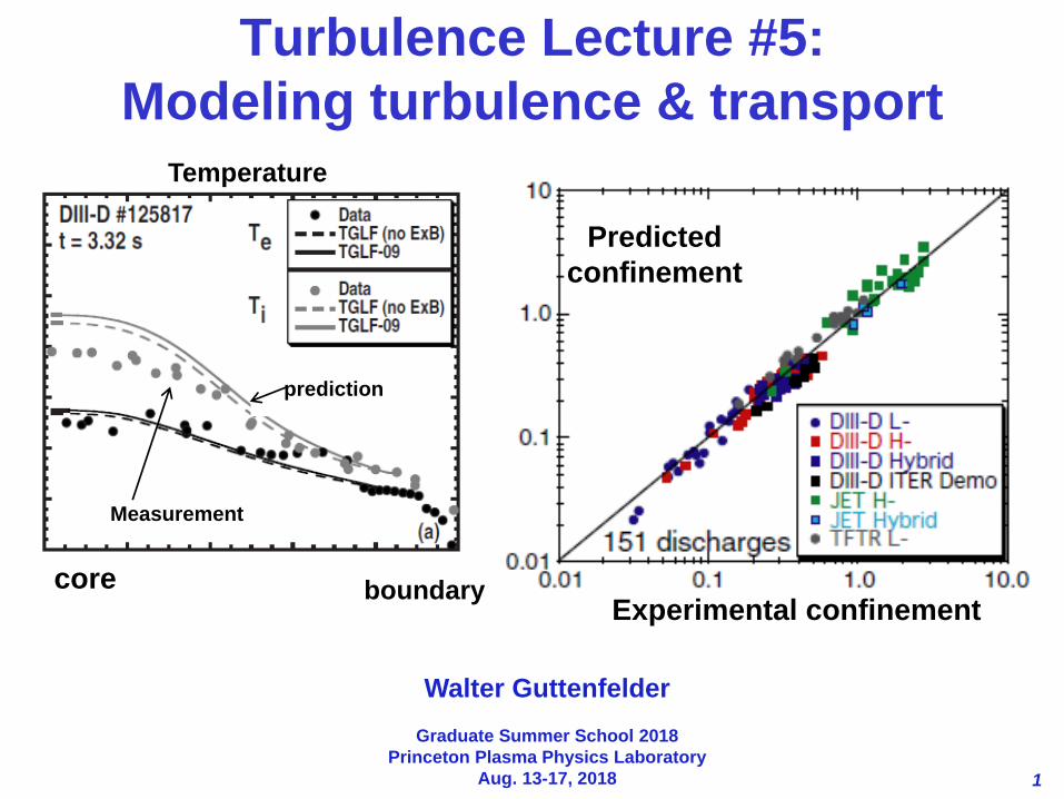
1 Turbulence Lecture #5: Modeling turbulence & transport Walter Guttenfelder Graduate Summer School 2018 Princeton Plasma Physics Laboratory Aug. 13-17, 2018 core boundary Temperature Measurement prediction Experimental confinement Predicted confinement
Transcript of Turbulence Lecture #5: Modeling turbulence & transport · Turbulence Lecture #5: Modeling...
1
Turbulence Lecture #5:
Modeling turbulence & transport
Walter Guttenfelder
Graduate Summer School 2018
Princeton Plasma Physics Laboratory
Aug. 13-17, 2018
core boundary
Temperature
Measurement
prediction
Experimental confinement
Predicted
confinement
2
Lecture #5 outline
• Simple Illustration of building a turbulent transport model
• Few examples of modern turbulent transport models
3
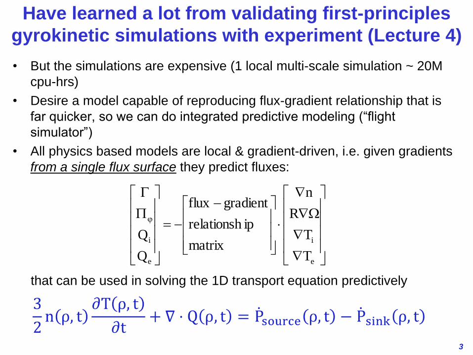
Have learned a lot from validating first-principles
gyrokinetic simulations with experiment (Lecture 4)
• But the simulations are expensive (1 local multi-scale simulation ~ 20M
cpu-hrs)
• Desire a model capable of reproducing flux-gradient relationship that is
far quicker, so we can do integrated predictive modeling (“flight
simulator”)
• All physics based models are local & gradient-driven, i.e. given gradients
from a single flux surface they predict fluxes:
that can be used in solving the 1D transport equation predictively
e
i
e
i
T
T
R
n
matrix
iprelationsh
gradientflux
Q
Q
4
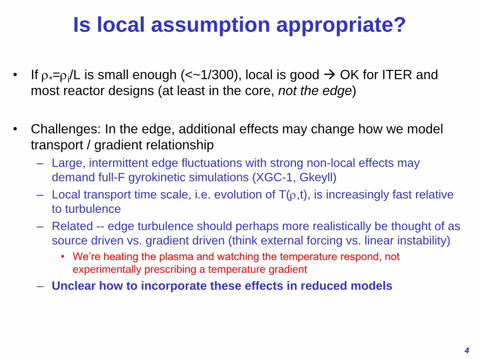
Is local assumption appropriate?
• If r*=ri/L is small enough (<~1/300), local is good OK for ITER and
most reactor designs (at least in the core, not the edge)
• Challenges: In the edge, additional effects may change how we model
transport / gradient relationship
– Large, intermittent edge fluctuations with strong non-local effects may
demand full-F gyrokinetic simulations (XGC-1, Gkeyll)
– Local transport time scale, i.e. evolution of T(r,t), is increasingly fast relative
to turbulence
– Related -- edge turbulence should perhaps more realistically be thought of as
source driven vs. gradient driven (think external forcing vs. linear instability)
• We’re heating the plasma and watching the temperature respond, not
experimentally prescribing a temperature gradient
– Unclear how to incorporate these effects in reduced models
5
TRANSPORT MODEL
DEVELOPMENT
6
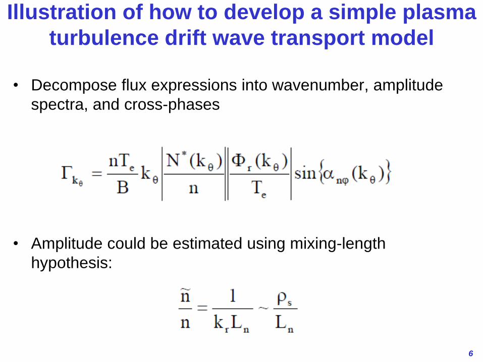
Illustration of how to develop a simple plasma
turbulence drift wave transport model
• Decompose flux expressions into wavenumber, amplitude
spectra, and cross-phases
• Amplitude could be estimated using mixing-length
hypothesis:
7
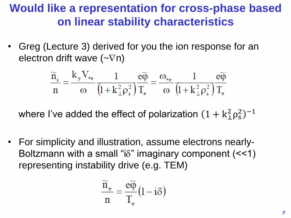
Would like a representation for cross-phase based
on linear stability characteristics
• Greg (Lecture 3) derived for you the ion response for an
electron drift wave (~n)
where I’ve added the effect of polarization 1 + k⊥2ρs
2 −1
• For simplicity and illustration, assume electrons nearly-
Boltzmann with a small “id” imaginary component (<<1)
representing instability drive (e.g. TEM)
8
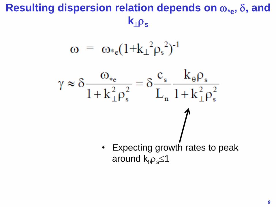
Resulting dispersion relation depends on w*e, d, and
krs
• Expecting growth rates to peak
around kqrs1
9
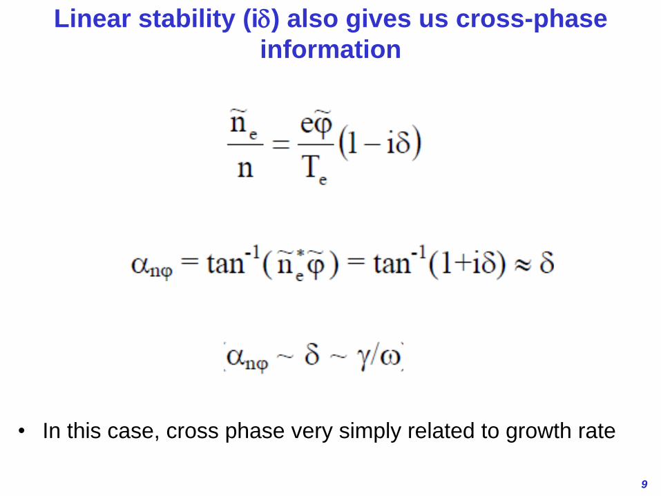
Linear stability (id) also gives us cross-phase
information
• In this case, cross phase very simply related to growth rate
10
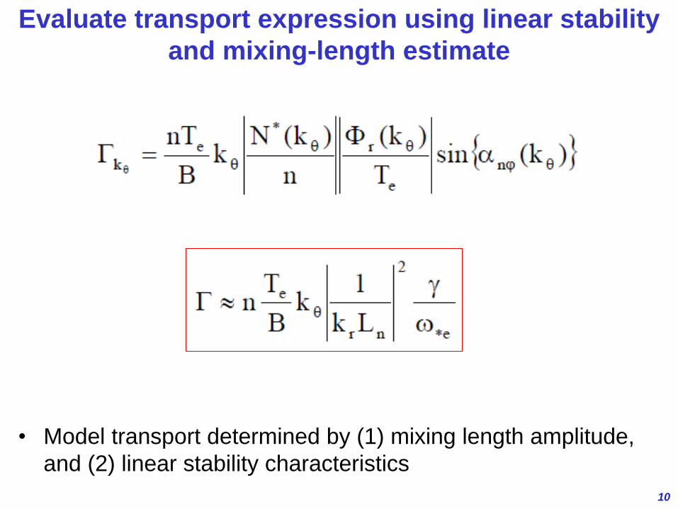
Evaluate transport expression using linear stability
and mixing-length estimate
• Model transport determined by (1) mixing length amplitude,
and (2) linear stability characteristics
11
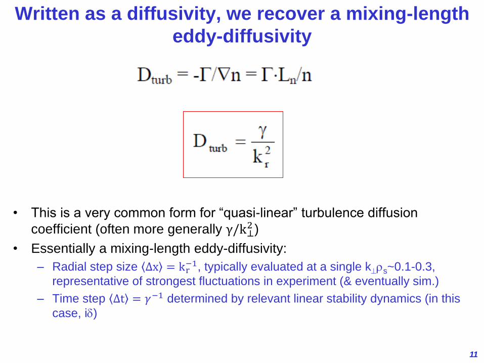
Written as a diffusivity, we recover a mixing-length
eddy-diffusivity
• This is a very common form for “quasi-linear” turbulence diffusion
coefficient (often more generally γ/k⊥2 )
• Essentially a mixing-length eddy-diffusivity:
– Radial step size Δx = kr−1, typically evaluated at a single krs~0.1-0.3,
representative of strongest fluctuations in experiment (& eventually sim.)
– Time step Δt = 𝛾−1 determined by relevant linear stability dynamics (in this
case, id)
12
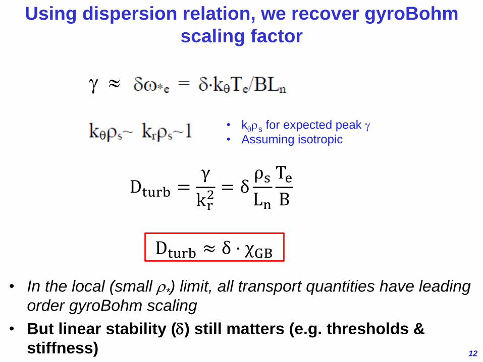
Using dispersion relation, we recover gyroBohm
scaling factor
• In the local (small r*) limit, all transport quantities have leading
order gyroBohm scaling
• But linear stability (d) still matters (e.g. thresholds &
stiffness)
• kqrs for expected peak g
• Assuming isotropic
g
Dturb =γ
kr2 = δ
ρsLn
TeB
Dturb ≈ δ ⋅ χGB
13
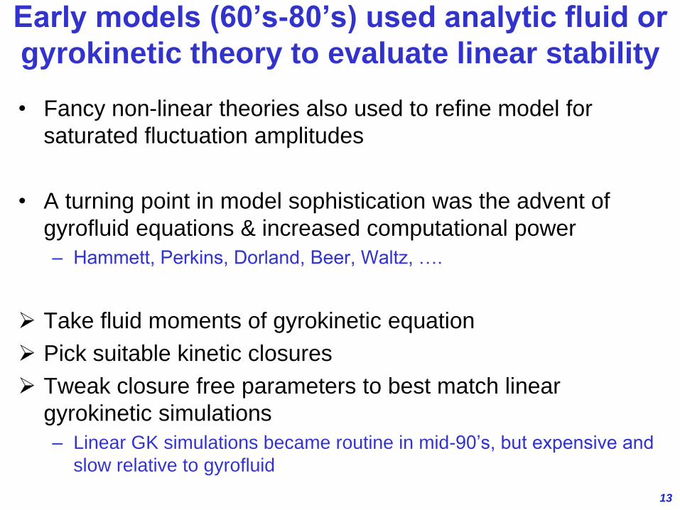
Early models (60’s-80’s) used analytic fluid or
gyrokinetic theory to evaluate linear stability
• Fancy non-linear theories also used to refine model for
saturated fluctuation amplitudes
• A turning point in model sophistication was the advent of
gyrofluid equations & increased computational power
– Hammett, Perkins, Dorland, Beer, Waltz, ….
Take fluid moments of gyrokinetic equation
Pick suitable kinetic closures
Tweak closure free parameters to best match linear
gyrokinetic simulations
– Linear GK simulations became routine in mid-90’s, but expensive and
slow relative to gyrofluid
14
MODERN TURBULENT
TRANSPORT MODELS
15
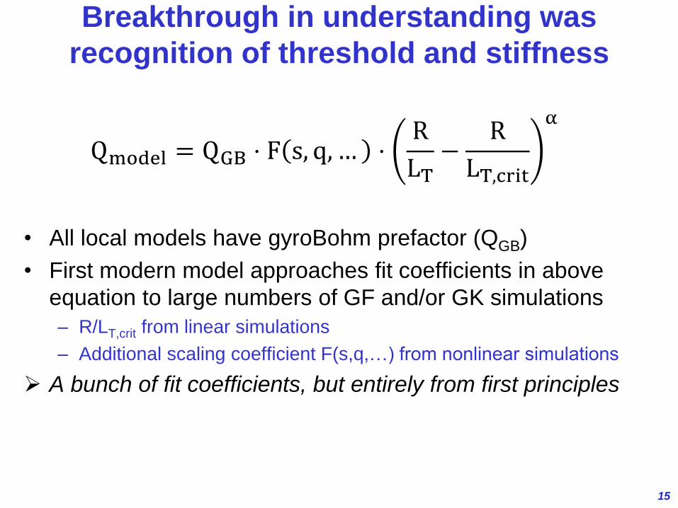
Breakthrough in understanding was
recognition of threshold and stiffness
• All local models have gyroBohm prefactor (QGB)
• First modern model approaches fit coefficients in above
equation to large numbers of GF and/or GK simulations
– R/LT,crit from linear simulations
– Additional scaling coefficient F(s,q,…) from nonlinear simulations
A bunch of fit coefficients, but entirely from first principles
Qmodel = QGB ⋅ F s, q, … ⋅R
LT−
R
LT,crit
α
16
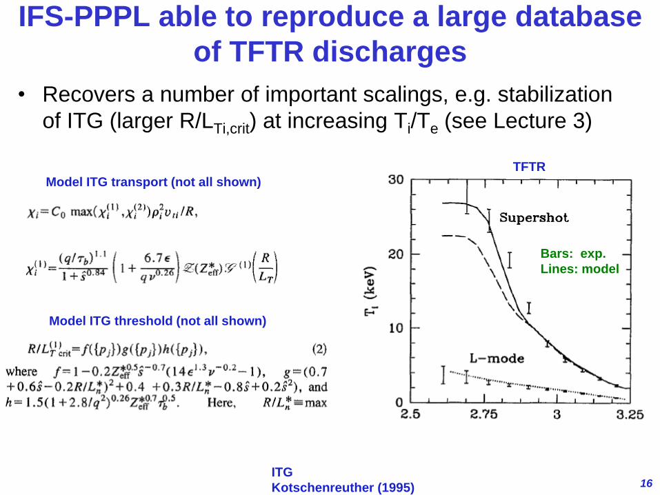
IFS-PPPL able to reproduce a large database
of TFTR discharges
• Recovers a number of important scalings, e.g. stabilization
of ITG (larger R/LTi,crit) at increasing Ti/Te (see Lecture 3)
ITG
Kotschenreuther (1995)
TFTR
Model ITG transport (not all shown)
Model ITG threshold (not all shown)
Bars: exp.
Lines: model
17
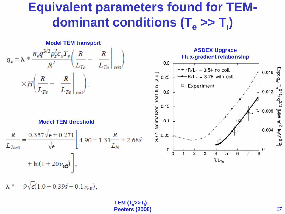
Equivalent parameters found for TEM-
dominant conditions (Te >> Ti)
TEM (Te>>Ti)
Peeters (2005)
Model TEM transport
Model TEM threshold
ASDEX Upgrade
Flux-gradient relationship
18
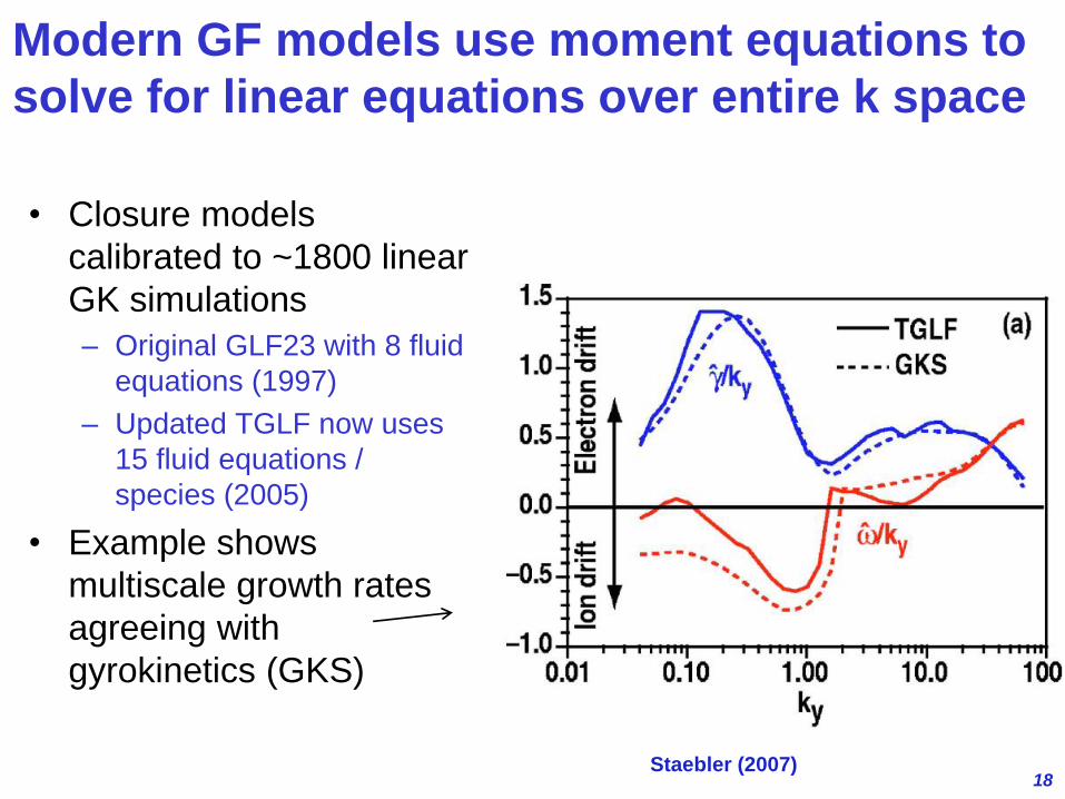
Modern GF models use moment equations to
solve for linear equations over entire k space
• Closure models
calibrated to ~1800 linear
GK simulations
– Original GLF23 with 8 fluid
equations (1997)
– Updated TGLF now uses
15 fluid equations /
species (2005)
• Example shows
multiscale growth rates
agreeing with
gyrokinetics (GKS)
Staebler (2007)
19
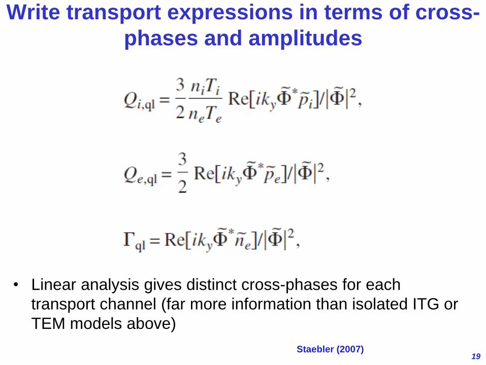
Write transport expressions in terms of cross-
phases and amplitudes
• Linear analysis gives distinct cross-phases for each
transport channel (far more information than isolated ITG or
TEM models above)
Staebler (2007)
20
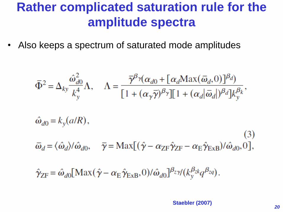
Rather complicated saturation rule for the
amplitude spectra
• Also keeps a spectrum of saturated mode amplitudes
Staebler (2007)
21
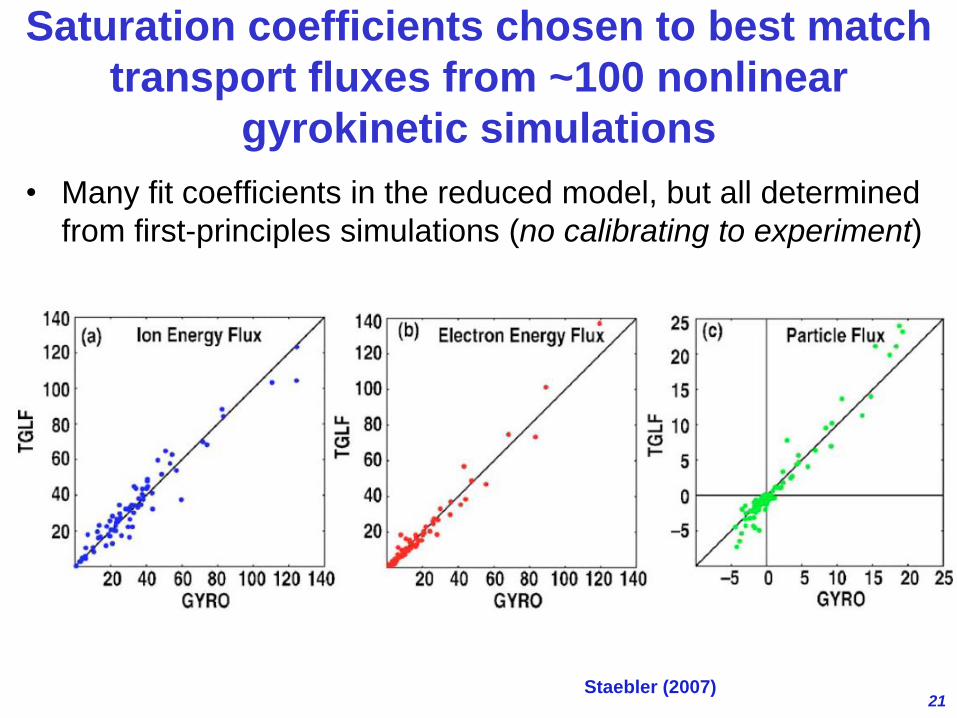
Saturation coefficients chosen to best match
transport fluxes from ~100 nonlinear
gyrokinetic simulations
• Many fit coefficients in the reduced model, but all determined
from first-principles simulations (no calibrating to experiment)
Staebler (2007)
22
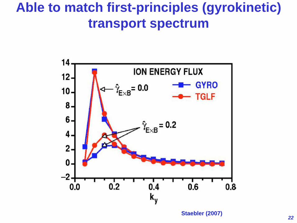
Able to match first-principles (gyrokinetic)
transport spectrum
Staebler (2007)
23
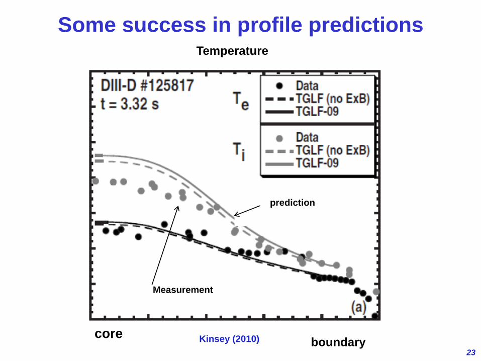
Some success in profile predictions
core boundary
Temperature
Measurement
prediction
Kinsey (2010)
24
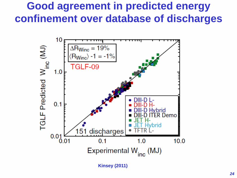
Good agreement in predicted energy
confinement over database of discharges
Kinsey (2011)
25
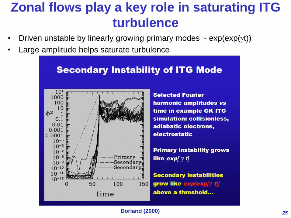
Zonal flows play a key role in saturating ITG
turbulence • Driven unstable by linearly growing primary modes ~ exp(exp(gt))
• Large amplitude helps saturate turbulence
Dorland (2000)
26
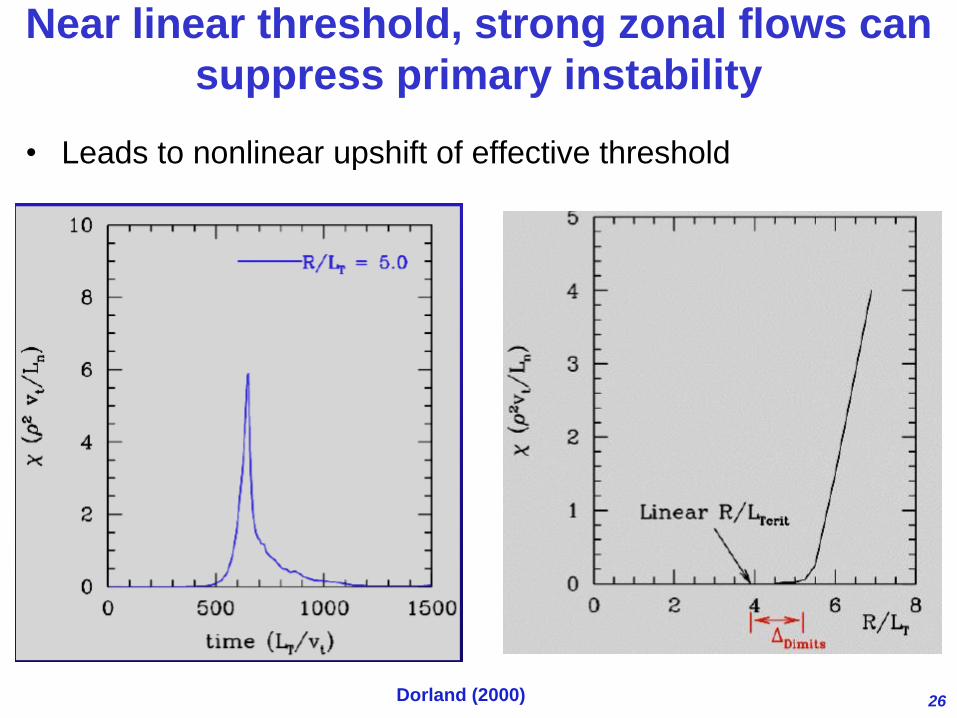
Near linear threshold, strong zonal flows can
suppress primary instability
• Leads to nonlinear upshift of effective threshold
Dorland (2000)
27
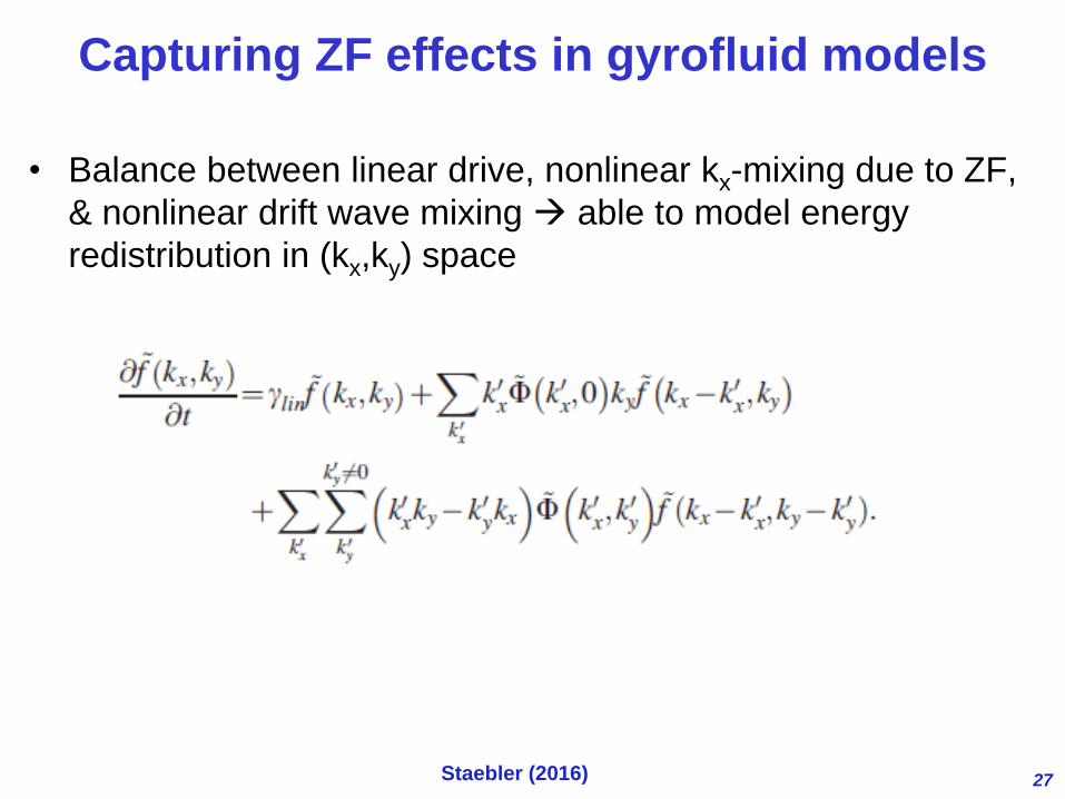
Capturing ZF effects in gyrofluid models
• Balance between linear drive, nonlinear kx-mixing due to ZF,
& nonlinear drift wave mixing able to model energy
redistribution in (kx,ky) space
Staebler (2016)
28
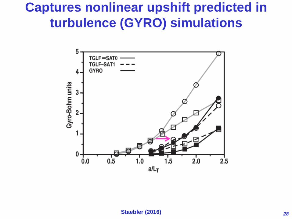
Captures nonlinear upshift predicted in
turbulence (GYRO) simulations
Staebler (2016)
29
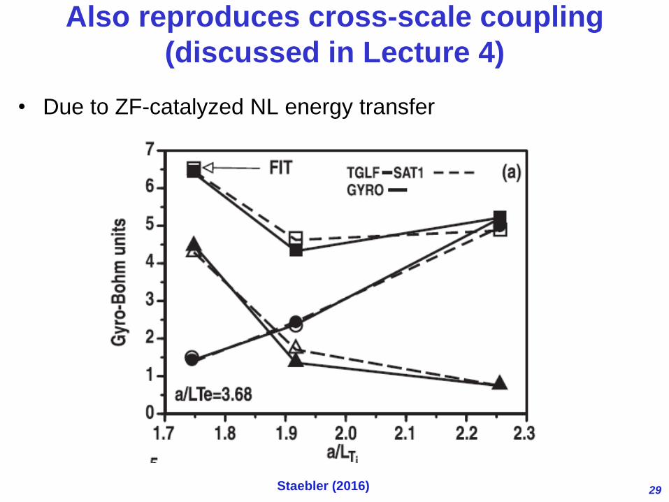
Also reproduces cross-scale coupling
(discussed in Lecture 4)
• Due to ZF-catalyzed NL energy transfer
Staebler (2016)
30
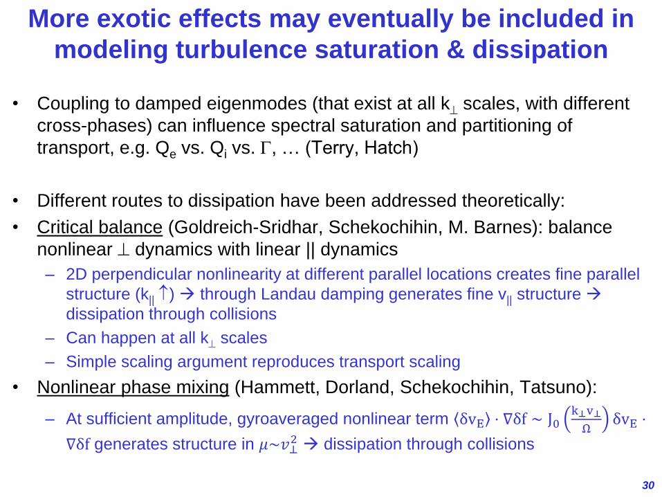
More exotic effects may eventually be included in
modeling turbulence saturation & dissipation
• Coupling to damped eigenmodes (that exist at all k scales, with different
cross-phases) can influence spectral saturation and partitioning of
transport, e.g. Qe vs. Qi vs. , … (Terry, Hatch)
• Different routes to dissipation have been addressed theoretically:
• Critical balance (Goldreich-Sridhar, Schekochihin, M. Barnes): balance
nonlinear dynamics with linear || dynamics
– 2D perpendicular nonlinearity at different parallel locations creates fine parallel
structure (k|| ) through Landau damping generates fine v|| structure
dissipation through collisions
– Can happen at all k scales
– Simple scaling argument reproduces transport scaling
• Nonlinear phase mixing (Hammett, Dorland, Schekochihin, Tatsuno):
– At sufficient amplitude, gyroaveraged nonlinear term δvE ⋅ ∇δf ∼ J0k⊥v⊥
ΩδvE ⋅
∇δf generates structure in 𝜇~𝑣⊥2 dissipation through collisions
31
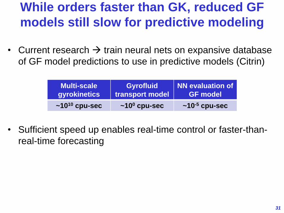
While orders faster than GK, reduced GF
models still slow for predictive modeling
• Current research train neural nets on expansive database
of GF model predictions to use in predictive models (Citrin)
• Sufficient speed up enables real-time control or faster-than-
real-time forecasting
Multi-scale
gyrokinetics
Gyrofluid
transport model
NN evaluation of
GF model
~1010 cpu-sec ~100 cpu-sec ~10-5 cpu-sec
32
Summary
• Magnetized turbulent transport models fundamentally use
quasi-linear calculation of cross-phases plus mixing-length
like saturation estimates
• Have shown a number of successes in reproducing first-
principles simulations
• As always, discrepancies (and failures) increase moving
towards the edge a frontier of turbulence and transport
modeling


