
Turbulence in Astrophysical and Laboratory...
55
Turbulence in Astrophysical and Laboratory Plasmas William Dorland Univ of Maryland, Univ of Oxford MIPSE, Univ of Michigan September 15, 2010
Transcript of Turbulence in Astrophysical and Laboratory...

Turbulence in Astrophysical and Laboratory Plasmas
William Dorland Univ of Maryland, Univ of Oxford
MIPSE, Univ of MichiganSeptember 15, 2010

Contributing Colleagues
Steve Cowley (UKAEA & Imperial College) Alex Schekochihin, M Barnes (Oxford Univ)Kate Despain (Maryland)T Tatsuno, R Numata, G Plunk (Maryland)Barrett Rogers (Dartmouth)Frank Jenko (Garching)Greg Hammett, David Mikkelsen (Princeton)Mike Kotschenreuther (Texas)Eliot Quataert, Stuart Bale (UC-Berkeley)Greg Howes (Univ of Iowa)
Keynes: “It is astonishing what foolish things a man thinking alone can come temporarily to believe.”
Overview
• Background
• A few successes:
• Nature of ion thermal transport: stiff
• Electron-gyroradius-scale fluctuations are interesting
• Multiscale algorithm developed for coupled turbulence and transport
• Gyrokinetic entropy cascade (perp phase-mixing)
• Gyrofluid revival? 1000x speedup in first-principles modeling
• Identification of Alfvenic solar wind turbulence
• Conclusion

Kinetic theory when (or )
!f
!t+ v ·
!f
!x
+ a ·
!f
!v
= C(f, f)
EM fields Two-particle collisions
ρ ≥ λ⊥λmfp ≥ λ

Kinetic theory when (or )
!f
!t+ v ·
!f
!x
+ a ·
!f
!v
= C(f, f)
EM fields Two-particle collisions
Boltzmann equation + Maxwell’s equations = kitchen sink
ρ ≥ λ⊥λmfp ≥ λ

Kinetic theory when (or )
!f
!t+ v ·
!f
!x
+ a ·
!f
!v
= C(f, f)
EM fields Two-particle collisions
Boltzmann equation + Maxwell’s equations = kitchen sinkVery frequently, the largest term in the equation is the acceleration due to the (self-consistent and/or imposed) magnetic field: leads to rapid gyration.
Take advantage of this, and work out asymptotically rigorous equations that describe all dynamics slower than the gyration: theory is known as “gyrokinetics”.
Two approaches: (1) conventional multiscale (2) Lie transform techniques
ρ ≥ λ⊥λmfp ≥ λ

Basic idea: Asymptotic, multiscale expansion
Expand Boltzmann and Maxwell equations in powers of epsilon, where
≡ ω
Ωc, Ωc ≡
qB
mc.

Basic idea: Asymptotic, multiscale expansion
Expand Boltzmann and Maxwell equations in powers of epsilon, where
≡ ω
Ωc, Ωc ≡
qB
mc.
Identify relevant physics at each order in epsilon (gyration, turbulence, thermodynamics) taking place at different space and time scales.

Basic idea: Asymptotic, multiscale expansion
Expand Boltzmann and Maxwell equations in powers of epsilon, where
≡ ω
Ωc, Ωc ≡
qB
mc.
Identify relevant physics at each order in epsilon (gyration, turbulence, thermodynamics) taking place at different space and time scales.
New qualitative features: for processes that are slow compared to the gyration, equations are reduced in dimensionality (from 6 to 5) but are integro-differential.
Conceptually, particles are replaced by rings whose radii are time-varying.
Interesting turbulent phenomena exist with eddies both large and small, compared to a typical “gyroradius”. Challenging to study!

Basic idea: Asymptotic, multiscale expansion
: Not described
: Point particles replaced by finite-sized “rings”
: Small scale dynamics (instabilities and fluctuations)
: Large scales slowly evolving
: Large scale moments close; no small-scale parallel nonlinearity
: Guiding center defined w/ this accuracy; limits field variation
: Perp scales smaller than a gyroradius treated faithfully
: Perp scales comparable to gyroradius “most natural” for theory
: Parallel scales of fluctuations comparable to equilibrium lengths
: Averaged quantities on large perp scales evolve slowly
ω > Ω
ω = Ωω ∼ Ωω ∼ 3Ω
∆ < ρ
∆ ∼ ρ
∆ ∼ ρ/
ν ∼ 3/2Ω
∆ ∼ ρ
∼ ρ/
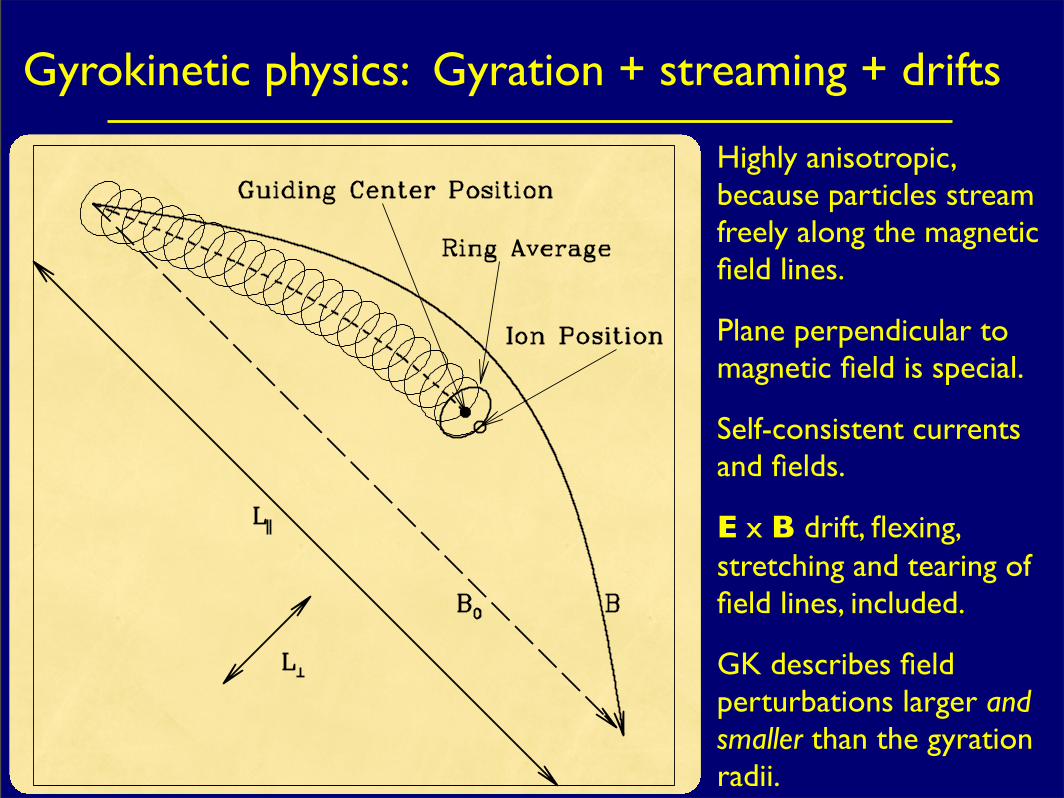
Gyrokinetic physics: Gyration + streaming + drifts
Highly anisotropic, because particles stream freely along the magnetic field lines.
Plane perpendicular to magnetic field is special.
Self-consistent currents and fields.
E x B drift, flexing, stretching and tearing of field lines, included.
GK describes field perturbations larger and smaller than the gyration radii.

Applications of gyrokinetics
Selected highlights
1. At high T, tokamak temperature profiles are stiff. ITG dominant
2. ETG turbulence can also be important, esp. when ITG is suppressed
3. Coupled turbulence/transport algorithm developed
4. Entropy cascade, turbulent heating
5. Gyrofluid revival? Fantastic GPU/CPU opportunity
6. Identification of solar wind fluctuations associated with Alfvenic cascade

At high temperature, transport is stiff
0
20
40
4 5 6
!ei/5
Expt. !ei
To
tal heat flux (
no
rmaliz
ed)
R/LT
Linear criticalgradients
Dimits shift
ITG+TEM; 2000-08

Offset-linear implies fast pulse propagation
1996

Offset-linear implies fast pulse propagation
1996

Offset-linear implies fast pulse propagation
1996
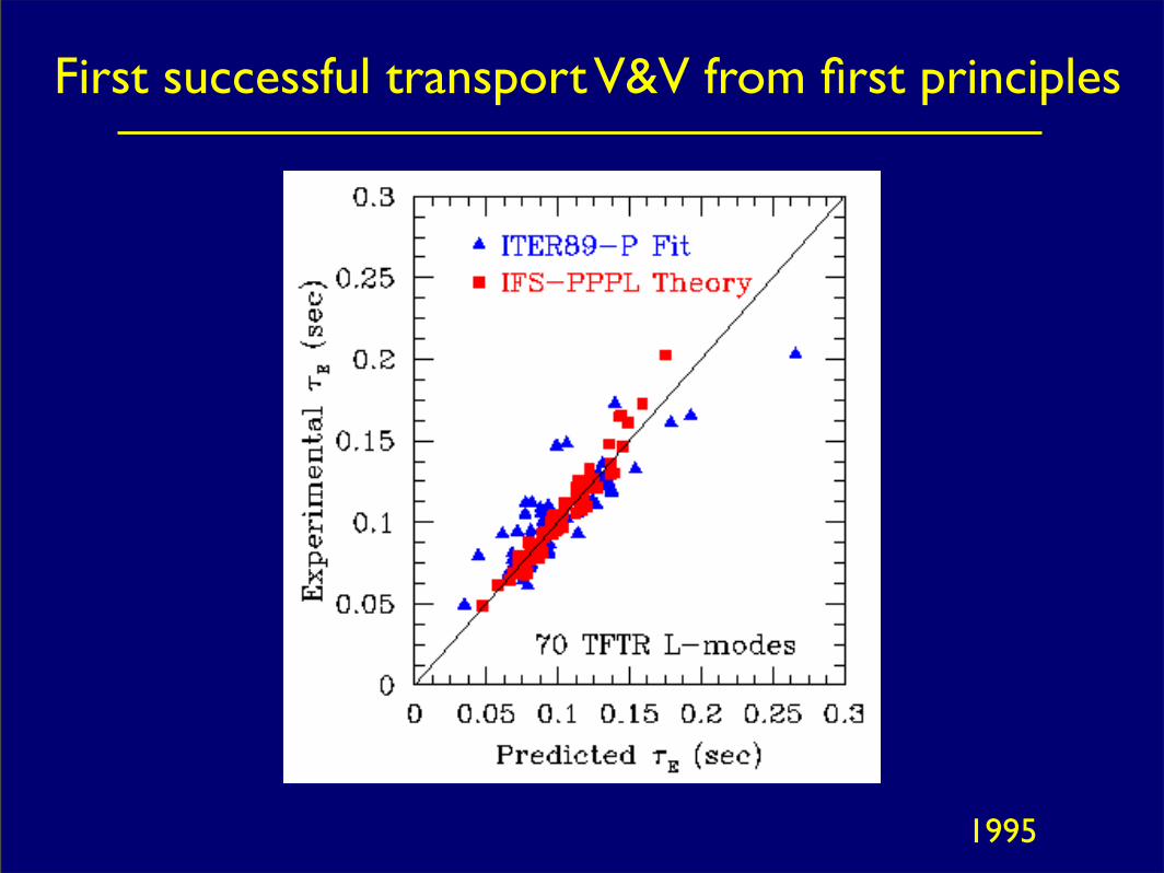
First successful transport V&V from first principles
1995

Observation of ETG fluctuations on NSTX
Recently, fluctuations predicted to be important (using continu-um gyrokinetic simulations) were observed in NSTX (PRL, 101, 075001, 2008).

Observation of ETG fluctuations on NSTX
Recently, fluctuations predicted to be important (using continu-um gyrokinetic simulations) were observed in NSTX (PRL, 101, 075001, 2008).
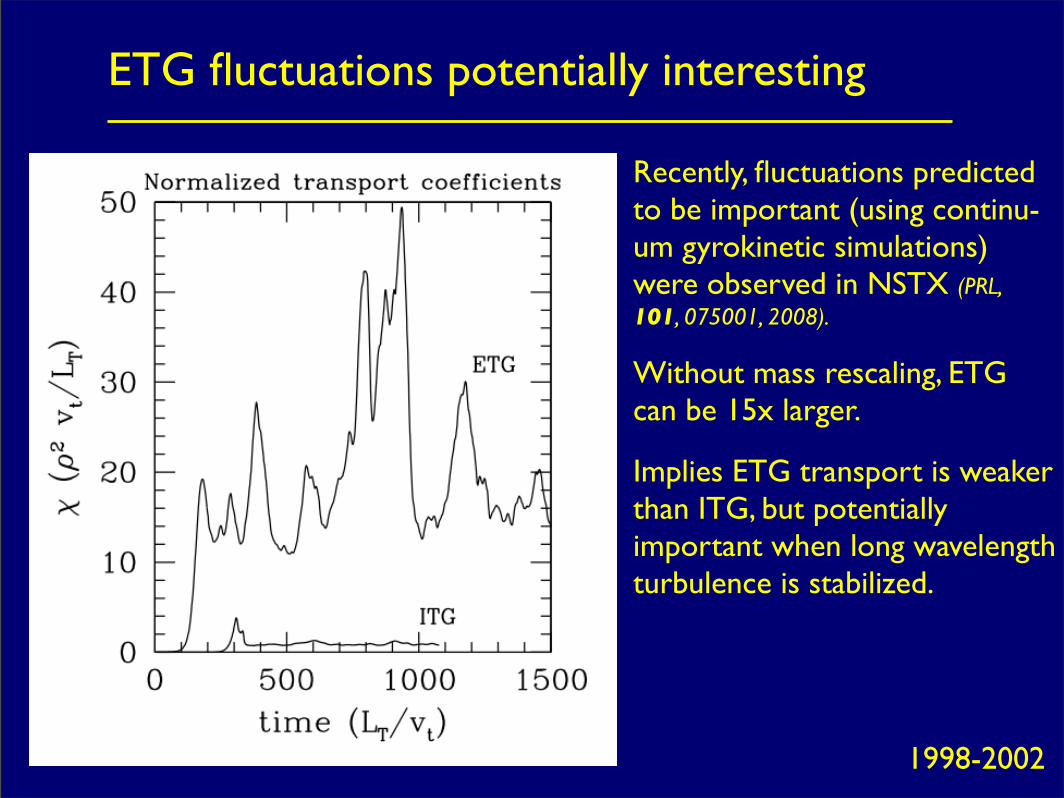
ETG fluctuations potentially interesting
Recently, fluctuations predicted to be important (using continu-um gyrokinetic simulations) were observed in NSTX (PRL, 101, 075001, 2008).
Without mass rescaling, ETG can be 15x larger.
Implies ETG transport is weaker than ITG, but potentially important when long wavelength turbulence is stabilized.
1998-2002

Stiffness of ETG varies; variation understood
Recently, fluctuations predicted to be important (using continu-um gyrokinetic simulations) were observed in NSTX (PRL, 101, 075001, 2008).
Without mass rescaling, ETG can be 15x larger.
Implies ETG transport is weaker than ITG, but potentially important when long wavelength turbulence is stabilized.
ETG stiffness varies strongly, understood theoretically (2002)

Coupled turbulence/transport algorithm (Barnes)

Direct simulation cost
Tem
p
•! Grid spacings in space (3D), velocity (2D) and time:
•! Grid points required:
•! Factor of ~1010 more than largest fluid turbulence calculations
•! Direct simulation not possible; need physics guidance
Time

Improved simulation cost
•! Field-aligned coordinates take advantage of a : savings of ~1000
•! Statistical periodicity in poloidal direction takes advantage of : savings of ~100
•! Total saving of ~105
•! Factor of ~105 more than largest fluid turbulence calculations
•! Simulation still not possible; need multiscale approach

Key results: turbulence and transport
(Boltzmann Eqn for short wavelength, mid-frequency turbulence)
1-D transport for slow background evolution depends on fluxes
(and sources, not shown)
Multiscale grid
Tim
e
Tim
e
Tem
p
Tem
p
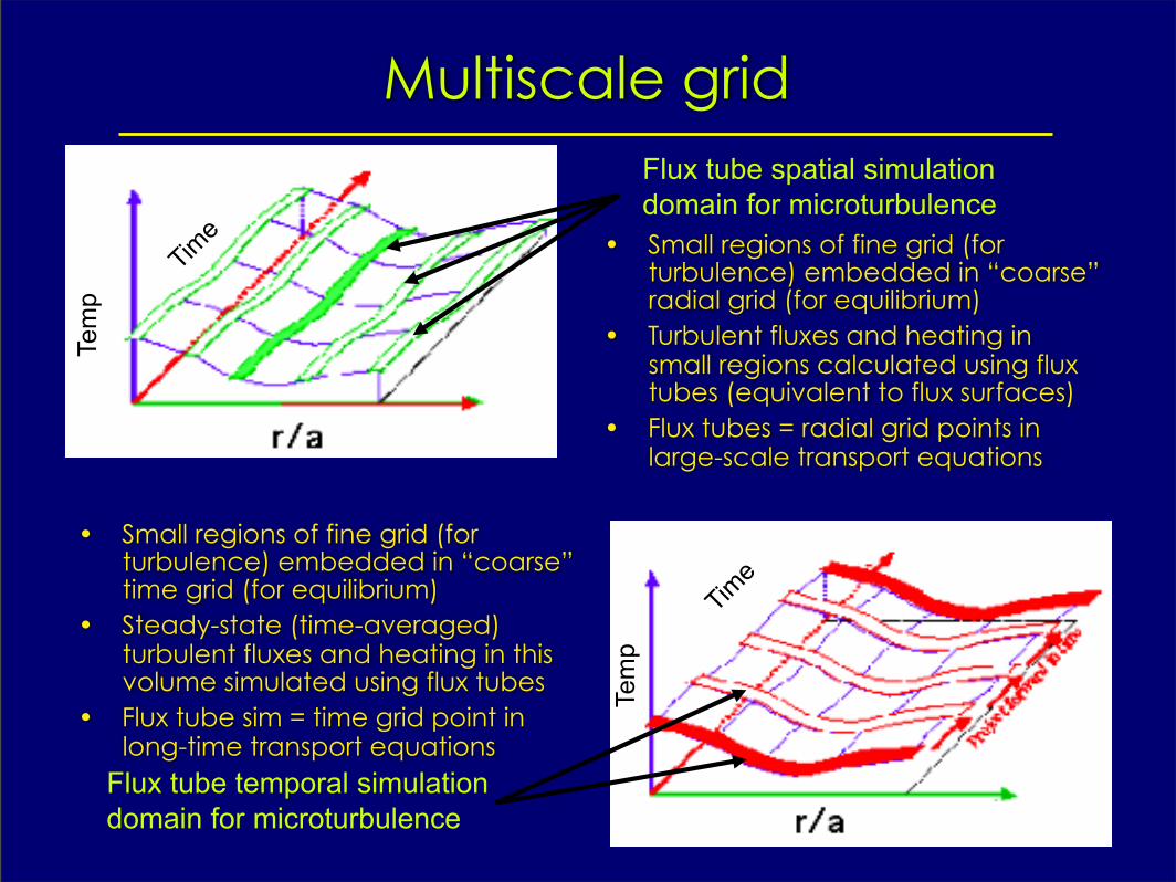
•! Small regions of fine grid (for turbulence) embedded in “coarse” radial grid (for equilibrium)
•! Turbulent fluxes and heating in small regions calculated using flux tubes (equivalent to flux surfaces)
•! Flux tubes = radial grid points in large-scale transport equations
Flux tube spatial simulation
domain for microturbulence
Flux tube temporal simulation
domain for microturbulence
•! Small regions of fine grid (for turbulence) embedded in “coarse” time grid (for equilibrium)
•! Steady-state (time-averaged) turbulent fluxes and heating in this volume simulated using flux tubes
•! Flux tube sim = time grid point in long-time transport equations

Flux tubes minimize flux surface grid points
Image of MAST simulation courtesty of G. Stantchev

Multiscale simulation cost
•! Grid spacings in radius and velocity (2D) roughly unchanged
•! Major savings is in time domain:
•! Required number of grid points:
•! Savings of ~103 over conventional numerical simulation
Coarse space-time grid
Tem
pera
ture
Tim
e
Turbulence:
Transport:

New topic in plasma turbulence
• Entropy cascade -- a newly discovered mechanism for turbulent plasma heating.

The cascade of entropy
• Energy and enstrophy cascades are well-known in 2D and 3D fluid turbulence.
• We have recently identified a new phenomenon which occurs in weakly collisional, magnetized plasma: the cascade of entropy.
• Before describing the new phenomenon, let’s review the simplest picture of the energy cascade in fluid turbulence...
Ek
k
stir
Inertial range
p =?
damp
Turbulent energy(cons.)
Wavenumber
∝ k−p
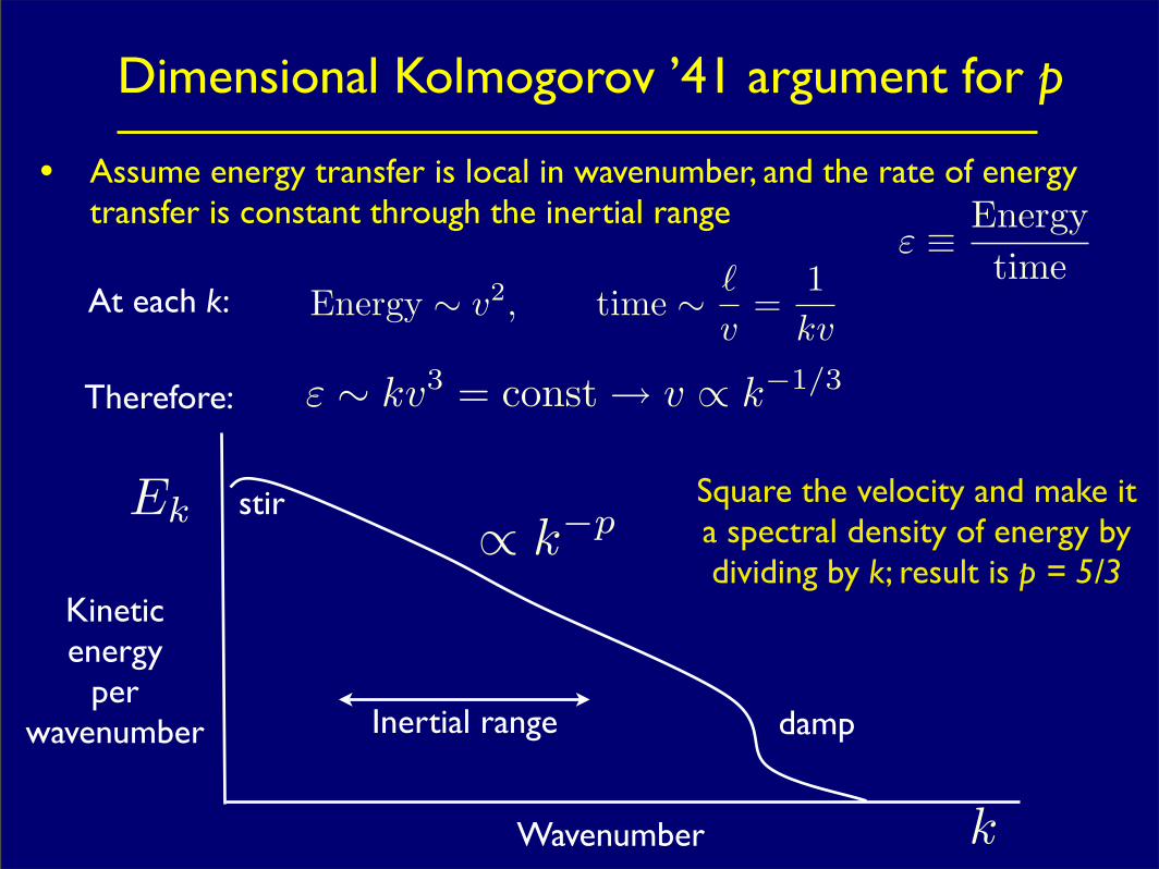
Dimensional Kolmogorov ’41 argument for p
• Assume energy transfer is local in wavenumber, and the rate of energy transfer is constant through the inertial range
ε ≡ Energytime
Energy ∼ v2, time ∼
v=
1kv
At each k:
Therefore: ε ∼ kv3 = const→ v ∝ k−1/3
Square the velocity and make it a spectral density of energy by dividing by k; result is p = 5/3
Ek
k
stir
Inertial range damp
Kinetic energy
perwavenumber
Wavenumber
∝ k−p

First step: Identify the conserved quantity[ies]
• In the inertial range, there is no stirring or damping.
• In this limit, it can be shown that the GK equations conserve
• Here, T0 is the temperature, F0 is the slowly varying part of the distribution function for species s, and the fluctuating quantities are indicated with deltas.
• It can also be shown that this conserved quantity reduces to the appropriate values in various limits, such as the fluid MHD limit
• It is this quantity that will be cascaded. Why do we talk about an entropy cascade?
E =
d3x
V
d3v
s
T0δf2
2F0
+
(δB)2
8π

Not quite entropy, but...
• Recall the definition of entropy:
• Here, the integration variable includes the space and velocity-space coordinates, kB is Boltzmann’s constant (taken to be unity from now), and the quantity f is the probability distribution function from kinetic theory.
• Upon expanding f = f0 + f1, and using spatial homogeneity to eliminate integrals over single powers of f1, one finds
• The quantity conserved by GK is a combination of magnetic field energy and S2, the second-order correction to the entropy. Hallatschek identifies the conserved quantity in terms of thermodynamic potentials (PRL, 2004).
S = −kB
f ln (f)dΓ
S0 ∝
f0 ln (f0)dΓ S1 = 0 S2 ∝
f21
f0dΓ

Predicted spectrum of ES entropy fluctuations
• Proceeding as before, define constant entropy flux, epsilon = Entropy/time
• Entropy ~ f 2 and time
• Complication: calculate self-consistent electric field scale by scale. Not easy! Use the physical intuition that v-space decorrelation , and solve Poisson’s equation to find the electrostatic potential:
• Put this all together, to find
• These scaling correspond to spectra for the non-Boltzman part of the entropy and the electrostatic potential as follows:
τ ∼ / <vE > ∼
(ρ/) 2/φ
v ∼
φ ∼ f
f ∼ 1/6 φ ∼ 7/6
Wh(k⊥) ∼ k−4/3⊥ , Wφ ∼ k−10/3
⊥

Numerical results consistent with expectations (Tatsuno)
Shown: three sims with increasing resolution
Decaying turbulence; will return to dissipation physics in a moment
Slopes generally consistent with estimated values
These are large runs -- thousands of processors on largest computers in US
10-8
10-7
10-6
10-5
10-4
10-3
10-2
10-1
100
1 2 5 10 20 50 100
W(k!)
/ W
ES
k! "
Wh
W#
k!-4/3
k!-10/3
(a)
(b)
(c)

Contours of f(v) at driving scale
This is a Maxwellian. There is no interesting structure in f(v).
What happens to f(v) at higher wavenumbers?-0.5
0
0.5
1
1.5
2
2.5
3
-3 -2 -1 0 1 2 3 0
0.5
1
1.5
2
2.5
3h(kx=1, ky=0)
v! / v
th
v|| / vth
h(kx=1, ky=0)

Reduce spatial scale 5x, see structure
-0.5
-0.4
-0.3
-0.2
-0.1
0
0.1
0.2
0.3
0.4
-3 -2 -1 0 1 2 3 0
0.5
1
1.5
2
2.5
3h(kx=5, ky=0)
v! /
vth
v|| / vth
h(kx=5, ky=0)
Begin to see structure in the perturbed distribution function in the perpendicular velocity direction.

Further reduce spatial scale, see more structure in f(v)
-0.3
-0.2
-0.1
0
0.1
0.2
0.3
0.4
-3 -2 -1 0 1 2 3 0
0.5
1
1.5
2
2.5
3h(kx=0, ky=10)
v! / v
th
v|| / vth
h(kx=0, ky=10)
Rate of structure formation is independent of collisions.
In the absence of collisions, could run time backwards and structure would disappear.
Collisions give irreversibility and heating -- with rate independent of ! ν

Small-angle collisions smooth v-space structure
• Give diffusion in v (second derivative in v-space)
• Important to have H-theorem for GK system (see PhD thesis of Barnes)
• Smoothing corresponds precisely to heating (Howes, 2008)
• Heating by nonlinear phase mixing is independent of collision frequency! And proportional to amplitude! Something fundamental and new -- missed by Landau.
• Scale at which irreversibility sets in given by balancing collisional smoothing against cascade to smaller scales:
δv⊥,c
vth∼ 1
k⊥,cρ∼ D−3/5,where D ≡ 1
ντρ.

Summary of perpendicular entropy cascade
• Particles with coincident gyrocenters but different gyroradii respond differently to the same electric fields, and contribute to the self-consistent fields differently.
• This leads to simultaneous structure formation at small scales in x and v.
• Even very infrequent collisions finally smooth f(v), resulting in irreversibility and turbulent heating, independent of the (finite) value of the collision frequency. Only the scale at which the heating occurs is affected by the specific value of the collision frequency -- not the rate of heating.
• (Note that the generation of small spatial scales alone would not result in heating in such weakly collisional gases -- collisional viscosity is irrelevant.)
• This source of heat may be important in a variety of contexts, such as in the case of the solar wind and in laboratory fusion experiments.
• Unlike Landau damping, this heating rate is amplitude dependent.

Gyrofluid revival? Fantastic opportunity
Inclusion of this physics brings GF into agreement with GK!
GF + GPU = Potential Trinity speedup of 1000x. Stunning.

Applications of gyrokinetics: Nature
The solar wind is a pressure-driven, outward flow of plasma from the sun.
The pressure should drop as the plasma expands, and the flow should stagnate.
Why doesn’t this happen? Perhaps turbulent heating -- in this case, gyrokinetic turbulent heating.
What we learn from solar wind may be applied to astrophysical systems.

Fluctuations in the solar wind
Fluctuations measured by Bale, et al., (2005).
At small wavenumbers, power spectra of electric and magnetic fields both have slopes ~ k -5/3

Fluctuations in the solar wind
Fluctuations measured by Bale, et al., (2005).
At small wavenumbers, power spectra of electric and magnetic fields both have slopes ~ k -5/3
Gyrokinetic simulations by Howes, et al., (2008)
At small wavenumbers, power spectra of electric and magnetic fields both have slopes ~ k -5/3
Numerical Dissipation

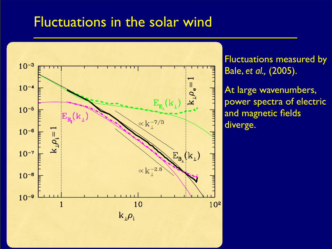
Fluctuations in the solar wind
Fluctuations measured by Bale, et al., (2005).
At large wavenumbers, power spectra of electric and magnetic fields diverge.

Fluctuations in the solar wind
Fluctuations measured by Bale, et al., (2005).
At large wavenumbers, power spectra of electric and magnetic fields diverge.
Numerical Dissipation
Gyrokinetic simulations by Howes, et al., (2008)
At large wavenumbers, power spectra of electric and magnetic fields diverge, in agreement with theory of kinetic Alfven wave turbulence.
Fluctuations in the solar wind
Fluctuations measured by Bale, et al., (2005).
At large wavenumbers, power spectra of electric and magnetic fields diverge.

Fluctuations in the solar wind
Fluctuations measured by Bale, et al., (2005).
At large wavenumbers, power spectra of electric and magnetic fields diverge.
Gyrokinetic simulations by Howes, et al., (2010)
At large wavenumbers, power spectra of electric and magnetic fields diverge, in agreement with theory of kinetic Alfven wave turbulence.

Conclusions
• Weakly collisional, magnetized plasma turbulence is important in a variety of contexts: fusion experiments, pressure-driven outflows
• A few results:
• Ion temperature profiles are stiff
• Electron-gyroradius scale turbulence is interesting
• First-principles transport modeling available now
• Entropy cascade occurs on scales smaller than gyroradius
• Electromagnetic fluctuation spectra in solar wind shown to be consistent with theoretical and numerical expectations, based on transition from Alfvenic to KAW turbulence.

The End


