!

NASA Contractor Report 4i47i

E--

!

r

c

i

z

Turbofan Forced Mixer

Lobe Flow Modeling

.i 1--Experimental and Analytical Assessment

T. Barber, R. W. Paterson,

and S. A. Skebe

CONTRACT NAS3-23039

OCTOBER 1988

https://ntrs.nasa.gov/search.jsp?R=19890004850 2018-06-03T07:14:42+00:00Z

F

[[

F

III

c

l

R

_T-T-

m

--T

Z.7_---7 ] _-

i

_ , ll___T----_--_--___ _-_--_, , _.-_

+_ l_[ i I _ L Ill _i -- .l '']l_l___

_ .... T_ _:_'l_l_'E _

NASA Contractor Report 4147

Turbofan Forced Mixer

Lobe Flow Modeling

I--Experimental and Analytical Assessment

T. Barber, R. W. Paterson,

and S. A. Skebe

United Technologies Corporation

Pratt & Whitney Engineering Division

East Hartford, Connecticut

Prepared forLewis Research Center

under Contract NAS3-23039

National Aeronautics

and Space Administration

Scientific and Technical

Information Division

1988

FOREWORD

The overall objective of this NASA program has been to develop and

implement several computer programs suitable for the design of lobeforced mixer nozzles. The analyses are based on linear or small

disturbance formulations. The analyses were applied to several mixer

lobe shapes to predict the downstream vorticity generated bydifferent lobe shapes. Data was taken in a simplified planar mixer

model tunnel to calibrate and evaluate the analysis. Anydiscrepancies between measured secondary flows emanating downstream

of the lobes and predicted vorticity by the analysis is fullyreviewed and explained. The lobe analysis are combined with an

existing 3D viscous calculation to help assess and explain measuredlobed data.

The program also investigated technology required to design forced

mixer geometries for augmentor engines that can provide forperformance requirements of future strategic aircraft. For this

purpose, available mixer design corre!ations were used to designseveral preliminary mixer concepts for application in a exhaust

system. Based on preliminary performance estimates, two mixerconfigurations were selected for further testing and analysis.

The results of the program are summarized in three volumes, all under

the global title, "Turbofan Forced Mixer Lobe Flow Modeling". Thefirst volume is entitled "Part I - Experimental and Analytical

Assessment" summarizes the basic analysis and experimental results aswell as focuses on the physics of the lobe flow field construed fromeach phase. The second volume is entitled "Part II - Three

Dimensional Inviscid Mixer Analysis (FLOMIX)" The third and last

volume is entitled "Part Ill - Application to Augmentor Engines".

pR'BI3EDiNG pAGE BLANK NOT FILMED

ill

ACKNOWLEDGEMENT

The authors wish to acknowledge helpful discussions with A11an Bishop

(NASA), Walter M. Presz, Jr. (Western New England College) and

Michael O. Werle (UTRC) _elative to the Formulation and conduct of

the study. Earl M. Murman (MIT) and George L. Muller (P&W) provided

guidance and assistance in the formulation of the analytical and

numerical FLOWMIX procedure. Roy K. Amiet (UTRC) developed the planar

analysis, PLANMIX. Appreciation is also expressed to 01of L. Anderson

(UTRC), Steve Zysman (P&W) and Bruce L. Morin (UTRC) for analytical

and experimental assistance, respectively, Edward M. Greitzer (MIT)

for reviewing the report and Thomas A. Wynosky who served as the

Pratt & Whitney Program Manager.

IV

SECTION

I .

II.

III.

IV.

V,

VI.

Vll.

TABLE OF CONTENFS

TITLE

FOREWORD

ACKNOWLEDGMENT

NOMENCLATURE

SUMMARY

INTRODUCTION

FORCED MIXER ANALYSIS

A General Concepts

B Planar AnalysisC Axisymmetric Analysis

D. Applications

DESCRIPTION OF EXPERIMENT

A Experimental Arrangement1 Mixer Lobe Cascade Facility2 Mixer Lobe Models

B Instrumentation

1 Laser Doppler Velocimetry2 Total and Static Pressures3 Flow Visualization

4 Boundary Layer Definition5 Experimental Technique

5 Data Analysis

RESULTS AND DISCUSSION

A. Experimental Observations

B.

C

1

23

45

67

MiMi

Data PresentationGeneral Observations

Mixer Lobe Flow Visualizat_on

Approximate AnalysisLow Penetration Sinusoidai Mixer

High Penetration Sinusoidal MixerAdvanced High Penetration ,ixer

xer Flow Analysisxer Flow Field Model

I. Circulations Calculations

2. Circulation and Mixing

SUMMARY OF RESULTS

CONCLUSIONS

REFERENCES

Page

iii

iv

vii

7

7

I0II

14

2929

2930

36

363839

3939

42

44

44

4445

465152

6273

8692

9297

99

101

103

SECTION

TABLE OF CONTENTS (Continued)

TITLE

APPENDICES

A. Viscous Marching AnalysisB. Lobed Mixer Coordinates

C. Code Input FilesD. Data Bases

E. Approximate Analysis

Page

105106

109I13

116143

v|

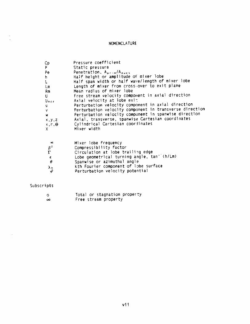
NOMENCLATURE

CpPPehLLmRmUUREF

u

v

w

x,y,zx,r,e

X

Pressure coefficient

Static pressure

Penetration, Ap_,m/Adu:_Half height or amplitude of mixer lobe

Half span width or half wave/length of mixer lobeLength of mixer from cross-over to exit planeMean radius of mixer lobe

Free stream velocity component in axial direction

Axial velocity at lobe exitPerturbation velocity component in axial directionPerturbation velocity component in transverse direction

Perturbation velocity component in spanwise directionAxial, transverse, spanwise Cartesian coordinates

Cylindrical Cartesian coordinatesMixer width

_2r

_k

Mixer lobe frequency

Compressibility factorCirculation at lobe trailing edge

Lobe geometrical turning angle, tan-'(h/Lm)

Spanwise or azimuthal anglekth Fourier component of lobe surfacePerturbation velocity potential

Subscripts

oO0

Total or stagnation property

Free stream property

vli

I. SUMMARY

This report describes a joint analytical and experimental investigation of

three-dimensional flowfield development within the lobe region of turbofan

forced mixer nozzles. The study represents a continuation of an effort

initiated by NASA and UTRC in 1977 to develop computational procedures for

predicting forced mixer nozzle mixing characteristics, thereby providing an

alternative to the empirical testing approach characteristic of the mixer

development process. The initial phase of that effort demonstrated that axial

vortex fields established at the lobe exit were responsible for the rapid

mixing observed in such nozzles and that when this secondary flow circulation

was used as a starting condition at the lobe exit plane, downstream nozzle

mixing could be predicted accurately. The objective of the current study was

to develop an analytical and experimental me_hod for predicting the lobe exit

flowfield, thereby providing, in conjunction with the mixing analysis, the

capability to compute engine flows from mixe," nozzle inlet to exit.

In the present analytical approach, a linearized inviscid aerodynamic theory

was used for representing the axial and seco_dary flows within the

three-dimensional convoluted mixer lobes and three-dimensional boundary layer

analysis was applied thereafter to account for viscous effects. The

experimental phase of the program employed three planar mixer lobe models

having different waveform shapes and lobe heights for which detailed

measurements were made of the three-dimensic,nal velocity field and total

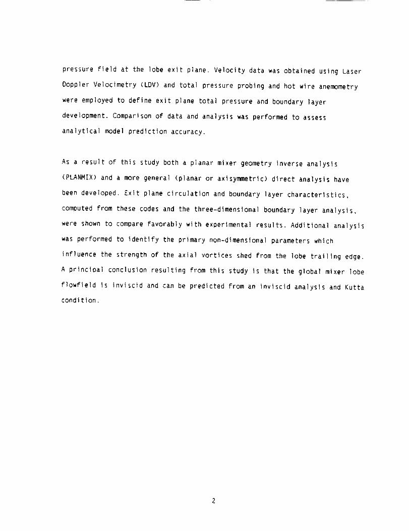
pressure field at the lobe exit plane. Velocity data was obtained using Laser

Doppler Velocimetry (LDV) and total pressure probing and hot wire anemometry

were employed to define exit plane total pressure and boundary layer

development. Comparison of data and analysis was performed to assess

analytical model prediction accuracy.

As a result of this study both a planar mixer geometry inverse analysis

(PLANMIX) and a more general (planar or axisymmetric) direct analysis have

been developed. Exit plane circulation and boundary layer characteristics,

computed from these codes and the three-dimensional boundary layer analysis,

were shown to compare Favorably with experimental results. Additional analysis

was performed to identify the primary non-dimensional parameters which

influence the strength of the axial vortices shed from the lobe trailing edge.

A principal conclusion resulting from this study is that the global mixer lobe

flowfield is inviscid and can be predicted from an inviscid analysis and Kutta

condition.

II. I NTRODUCTIGN

The overall research problem addressed in this study was the development of an

analytical method for predicting three-dimensional flow development within the

convoluted lobes of forced mixer nozzles installed in modern commercial

turbofan engines. The design of these forced mixer lobes has been

traditionally accomplished by using experimental correlations to relate mixer

performance to a variety of geometrical parameters. This process is typically

an iterative one, relying heavily on experimental verification. While this

process has been reasonab}y successful, little insight has been gained as to

the driving flow mechanisms involved and how to design the lobe surfaces so as

to optimize the mixing process. The formulation of an analytica} procedure is

critical to the development of improved mixer designs for use in such engines

and in the numerous additional applications of mixers which have been recently

identified.

Turbofan engine mixer technology is well established as a means for reducing

aircraft jet noise while at the same time achieving a measurable thrust

improvement. In addition to reducing noise by rapidly mixing out the high

axial velocity primary stream fluid with the lower velocity secondary stream,

the mixer reduces peak nozzle exit plane temperature, which is an important

consideration for certain engine applications. Recent research (Ref. l)

conducted at Western New England College and UTRC under NASA sponsorship has

shown mixer lobes can dramatically improve the performance of ejectors such as

suggested for use in advanced exhaust systems. Other applications of mixer

lobe axial vorticity flow control have been also identified (Ref. 2,3). These

involve airfoil stall and separation alleviation. Initial efforts at

analytically investigating the flow in mixer nozzles were performed in

conjunction with "benchmark" experiments (Ref. 4_5) that obtained a detailed

description of the flow within a model turbofan forced mixer nozzle. Laser

Doppler Velocimetry (LDV) was employed to define the three-dimensional

velocity field between the lobe exit plane and the nozzle exit. These

experiments have determined that the mixing process is dominated by the

secondary flow generated within the lobe region of the flow. Anderson et al.

(Ref. 6,7) have proposed several sources for the secondary flow and lumped

them together under a "generic" vorticity label. This vorticity source has

been analytically simulated in a viscous marching analysis and has reproduced

the observed flow mixing patterns and magnitudes.

Whereas previous research studies conducted at UTRC and NASA Lewis Research

Center have shown that three-dimensional viscous computational procedures can

be employed to calculate the nozzle mixing downstream of the mixer lobe exit

plane, no analytical method existed at the outset of the present study for

predicting the lobe exit plane flow field. Furthermore, these prior studies

showed that the success of the mixing calculation in predicting the

experimental nozzle mixing data was critically dependent upon the correct

definition of the secondary flow circulation existing at the exit of each

mixer lobe segment. Similar studies were conducted during the present program

using the PEPSI-M Parabolized Navier Stokes code and applying it to the data

cited in reference 2. These results substantiate the earlier results of other

researchers and indicate the magnitudeof the sE_condaryflow induced

circulation field is directly related to the loL:e shape. The highlights of

this study are presented in AppendixA. As a result of this research, it was

clear that the major problem remaining in the construction of an overall

prediction and design analysis system for turbofan engine forced mixers was

the prediction of the flow field developmentwi';hin the three-dimensional

convoluted lobes.

The outstanding issues to be resolved in this r_search programwere: how is

the secondary flow field generated over the lob,_ surface, is this process also

largely inviscidly dominatedand can a simplified analytical procedure be

constructed to predict the lobe exit plane flow field for a wide class of

convoluted geometries? This report, as Part 1 oi:: a three part series,

addresses these issues by developing an invisciJ numerical procedure for

predicting the flow over the lobe and thereby generating the necessary exit

plane secondary flowfield. The accuracy of the _nalytical model is then

assessedwith benchmarkdata bases generated in the present program for

selected mixer geometries. A specific focus of this study was to use

information gained from the joint analytical anJ experimental research to

design an advancedconfiguration which produces higher levels of axial

vorticity and circulation. Testing of this configuration and corresponding

code predictions assisted in the formulation of recommendationsrelative to

future research directions in the area of mixer technology. Finally, this

report constructs a modelof the flow mechanismwithin the lobe region and in

the interface region between the lobe and the downstreammixing duct.

The approach was a combined analytical and experimental effort. The analytical

approaches developed herein are based on linear inviscid theory. Two computer

codes, PLANMIX and FLOMIX, were developed. The viscous flow development over

the lobes was then determined using an ex post facto three-dimensional

boundary layer analysis. Lobe testing was also conducted to investigate the

lobe flow field and to provide data for assessing the analyses. An

experimental data base was generated: LDV techniques defined the three-

dimensional velocity field and pitot probes defined total pressure

distributions at the lobe exit plane. Lobe circulation levels and exit plane

boundary layer characteristics were developed from this data. An approximate

analysis was developed for identifying scaling parameters For lobe circulation

and to assess waveform geometry effects on circulation.

The major conclusion of this study is that the linear inviscid analyses are

able to predict the lobe exit plane circulation with the coupled boundary

layer analysis, thereby predicting the shear layer development on the lobe

surface. For the three specific lobe models tested, these predictions were

found to be in reasonable agreement with experiment. Additional analyses

identified the primary parameter affecting the exit plane circulation for

straight-ramped lobes as the ratio of the lobe amplitude squared to lobe

length. From this result, it is concluded that the steepest ramp angle that

can be achieved without separation maximizes the induced circulation.

Futhermore, it was also concluded from studying the effect of mixer waveform

on circulation that parallel-sided configurations are inherently superior to

nonparallel configurations such as sinusoidal or triangular. Experimental data

confirmed these predictions regarding both lobe amplitude and waveform. It was

found that mixer lobe performance can be adversely affected by boundary layer

buildup in the interior peak or trough region cf the lobes, thereby reducing

their effective lobe amplitude and consequently the circulation shed into the

wake.

The analytical and experimental phases of this study have resulted in an

improved understanding of the mechanisms driving the lobe flowfield and has

produced a validated code for integration into an overall mixer nozzle design

analysis.

III. FORCEDMIXER ANALYSIS

A. General Concepts

The development of an analysis to predict the Flow over a mixer lobe is

inherently an extremely complex problem. The flow field is fully

three-dimensional, may have different energy levels between the mixing streams

and can be dominated by viscous dissipation effects. A complete numerical

solution of the Navier-Stokes equations still _epresents a major challenge,

both in grid generation and in resolving the thin shear layers over the lobe

surface. A more tractable approach, however, considers a zonal treatment,

wherein local regions are analyzed using simplified procedures. The analytical

approach pursued in this study has been built on the results of Anderson et

al. by exploring the source of "generic" vorticity and modeling it within the

basic conservation laws. The "flap" vorticity concept, schematically shown in

Figure I, models the lobe as aperiodic system of cambered airfoils. Applying

to each airfoil a Kutta condition at the trailing edge determines the inviscid

lift distribution and sets up the observed trailing edge secondary flow field.

The effects of viscosity are then accounted For using an ex post Facto

three-dimensional boundary layer analysis.

Figure 1

CORE FLOW

FAN FLOW RADIAL FLOW

(a) BASIC FLOW TURNING (b) RADIAL FLOWORIENTATION

Secondary Flow Generation, Turning (Flap) Vorticity Model

Two different inviscid analytical approaches have been formulated and used in

this study. Each procedure assumes the local flow to be irrotational and both

apply local linearizations to simplify application of the tangency boundary

condition from the convoluted mixer lobe surface to some mean surface

representation. The first is a planar indirect analysis called PLANMIX that

uncouples the spanwise dependence by assuming a sinusoidal waveform lobe

shape. The latter analysis is a planar and axisymmetric direct analysis called

FLOMIX which is capable of treating arbitrary lobe geometries and mixing of

streams with unequal total pressures and total temperatures. The simpler

PLANMIX code was used to validate the more complex FLOMIX code. Complete

documentation of each analysis can be found in References 8-11, but a brief

description is provided below. Specific applications of the programs are also

presented and these configurations are subsequently examined in the

experimental portion of this document.

In the Following design, analysis and data _ections of this report, an (x,y,z)

Cartesian coordinate system oriented with t_e x axis in the primary flow

direction, the y axis in the transverse or ,/ertical direction and the z axis

in the spanwise or lateral direction. The c.)ordinate origin is centered along

the lobe crest (z=O) anC vertically at the half height (y=O). All coordinates

have been normalized by L, the lobe half-wave length. The corresponding

velocity components are ( u + U_ ), v, w where u, v, w are velocity

perturbation components from the free stream Flow. The velocity components, as

presently in the text, will be normalized ty the free stream velocity U_ .

Z,_J

x,(u ,- Uo:)

A. Planar Analysis

The planar potential analysis (Ref. 8), called PLANMIX, is an inverse

procedure constructed to assist in the design of idealized lobes for a planar

low speed test facility. The analysis assumes the flow is both incompressible"

and irrotational. A flow solution in terms of the velocity potential can be

determined from Laplace's equation_ The PLANMIX analysis idealizes the mixer

lobe by unwrapping it so that the planform forms a corrugated flat plate in

the y:O plane. The linearization assumption furthermore implies that the lobe

height is small compared to all other length scales in the problem.

In the present case, a further restriction is imposed by assuming the lobe

surface is a sinusoidal cross-sectional shape, thereby removing the spanwise

indeterminancy. Solutions to Laplace's equation can always be obtained from

superposition of singularities, i.e., point sources (monopoles), doublets,

vortices. For an incompressible flow, a doublet distribution of specified

strength along the flat plate will uniquely define the lobe height and

therefore its shape. The surface height of a lobe h(x,z) can be determined

from the following expression:

X

h(x,z) = cos (_cz) f v (_, O, O) d_ (1)

J s__L--00 UCXJ

lO

where vs is the transverse component of the perturbation velocity defined in

terms of the dipole loading function

I/2f(x) : R (P JLm-xl) exp (-P JLm-_}) (2)

is the frequency of the mixer lobe, U_is the free stream velocity, x and z

are the axial and spanwise distance, respectively, P, the axial scaling length

and R, the loading amplitude. Because of the linearity of the problem,

proportional increases in R resuTt in a propo_tionally higher mixer lobe. The

choice of loading function is somewhat arbitrary, however, its strength was

chosen to be zero at the lobe trailing edge (<=0.) to satisfy the Kutta

condition. The loading function choice was based on linear airfoil theory and

exhibits the expected square root decay.

C. Axisymmetric Analysis

In contrast to the above planar inverse analysis, the FLOMIX axisymmetric

analysis (Ref. 9-11) solves for the flow over a given lobe contour. It also

removes many of the geometrical and flow modeling restrictions previously

imposed in order to more closely model the a::tual environment of a forced

mixer found in current generation gas turbine installations. More

specifically, the mixer lobe geometry is not limited to sinusoidal

cross-sections, the lobe flow field analysis includes the effects of the

adjacent centerbody and fan nozzle walls shown in Figure 2, and the effects of

power addition and compressibility are also simulated. A potential flow model

is still applicable if the inlet flows can Ue considered as two separate

irrotational regions divided by a vortex sheet. In such an analysis, the wake

must be dynamically tracked and two separate velocity potentials considered.

11

MIXER

Figure 2 Schematic Cutaway View of Forced Mixer Installation in a Turbofan

Engine

The FLOMIX is a control volume analysis developed in cylindrical Cartesian

coordinates, aligned to the engine centerline. A novel procedure is followed

by solving the flux balanced equations by locating the intersections of the

geometry with the regular rectangular mesh. This procedure is schematically

shown in Figure 3. Small disturbance approximations are applied to linearize

compressibility effects, i.e., the mass flux vector is approximated

by:

2 l

pv = (1. +t3 _ ) ] +¢ 1 +---@8 iex x r r r

(3a)

#z = I. - MZ= , (3b)

and the convoluted lobe surface is approximated by an axisymmetric surface of

mean radius Rm (x). This latter linearization permits one to uncouple the

spanwise dependence (8) through a Fourier modal analysis

NH

e(x, r, 8) = _ g (x,r) h (@) (4)k=l k K

12

FLOW CELL

"i"

J

I ]

4

J

Ii

I, i

; Iit

SURFACE CELL

Figure 3 Mixer Geometry Definition on a Cylindrical Cartesian Mesh

The solution is now determined in terms of several axisymmetric potentials

g, (x,r) with a Kutta condition and a Flow tangency boundary condition

imposed for each kth mode. The tangency ccndition can be shown to be

equivalent to an effective flux condition applied on the mean surface Rm(x)

' l

g (x,Rm _) : )k (x) + --- )- > .}k

r k 2 --"_--" n

k 2R m j n

(x) g (x,r) [(6c) - 6c)] (5)

J

where Xn , k', are the modal shapes and c,1opes of the various Fourier

modes of the mixer lobe. The leading term in Eq. (5) is the classical

two-dimensional contribution, while the l_tter term is the three-dimensional

spanwise term that couples the individual (k) modes. The orientation of X and

Rm are schematically shown in Figure 4. C(:,mplete details regarding the

solution procedure can be found in (Ref. _il).

13

Figure 4 Definition of Lobe Geometrical Parameters for Fourier Analysis

D. Applications

The PLANMIX inverse analysis was used to generate coordinates for two mixer

lobe configurations: one, a low penetration design that was consistent with

the linearization assumptions used in the analysis and the second, a high

penetration design chosen to examine the limits of the model's applicability.

In this case reference to lobe penetration refers to the degree of projection

of the core or inner flow into the bypass or outer stream. In classical mixer

terminology, this would be termed the flow turning (h/Lm), rather than the

penetration Pe which is an area ratio parameter. The code geometrical

parameters for the low and high penetration sinusoidal lobes are given below

and a side view of both is given in Figure 5.

14

AMIET F(X)= R ,_ X e11 2

Figure 5 NASA Sinusoida] '4ixerCascade Designs ] and 2

A complete tabulation of their coordinates is given in Appendix B. A plot of

the solutions for these mixer lobes, expressed in terms of axial distribution

of the linearized pressure coefficient (CpL = -2u/U_ ), iS shown in Figures

6(a) and 6<b). The axial pressure gradient is produced by the surface

curvature at the break from the planar _urface. The return to free stream,

CpL=O.O, iS driven by the trailing edge Kutta condition. The spanwise

gradient inviscidly drives the flow fron the crest (8' = 0.) to the trough

(8' = 1.0), where 8' is the reduced spar_wise coordSnate 8' = z / L = _/_o.

If the Flow solution was displayed in terms of the actual Cp, the lower order

contributions of v and w would result in a nonzero value of Cp at the lobe

trailing edge.

Low Penetration High PenetrationLobe Lobe

h/Lm 0.9 0.4

h 0.500 2.000

P 0.215 0.215

R 0.02209 0.8839 = 4 (.02209)

15

O5

CpL

oo ,

-05 _

CREST

TROUGH

[ J J_. J4 6

(al LOW PENETRATION MIXER

8 1 0

CpL

io-

05 -

-.o5

z= o f _,

5O

\\

/\ /

_,75 /

\ ]/

\ ]1.O

-_o- T T T T0 .2 4 6 ,8

AXIAL DISTANCE X/Lm

(bl HIGH PENETRATION MIXER

CREST

TROUGH

t.O

Figure 6 PLANMIX Calculated Pressure Coefficient on Mixer Lobe Surface

16

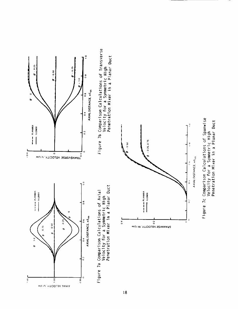
A calibration check of the FLOMIX analysi_ was made by calculating the high

penetration mixer lobe using the coordinates obtained From the PLANMIX inverse

analysis. The FLOMIX program can be used _o simulate a planar configuration by

modifying the lobe coordinates so that thE;_ mean radius Rm in the axisymmetric

mode is sufficiently large (Rm>> O). The fan nozzle and centerbody walls were

assumed planar and sufficiently displaced so that no wall interaction effects

were present. FLOMIX perturbation velocit,_ component calculations, shown in

Figures 7a, b, and c, are compared to the PLANMIX results. The two solutions

are essentially identical. Further validal;ion of the FLOMIX code are presented

in References 5 and 6, where calculations for the lobed mixer for the Energy

Efficient Engine (E3) in a powered enviroHment are compared to experimental

data (Ref. 12). Considerable agreement wa_;obtained although this case pushed

the limits of the small disturbance theorJ.

The validated FLOMIX program was used to _esign an advanced high penetration

lobed mixer, taking advantage of the experimental configuration base that was

obtained in the E3 program. The mixer cross-sectional contours, formed by

radii and circular arc segments, tended t:)be less peaked than the sinusoidal

type lobe section. A variation on one of the better performing designs was

adapted from an axisymmetric to a planar Format. Several Key geometrical

parameters were preserved in this adaptation in order to be consistent with

the empirical design procedure used in the original axisymmetric design.

Referring to the nomenclature in Figure 8, the specific procedure that was

followed is:

17

o

x

i_xz =E

I Ii,I

• I I

,_,N/A '_,J.IDO'I3A 3SEI3ASN'ffEI.I. _

i Li __z

_°!

=, / /

!.a o

_N N A.I.IDO'I3A qVIXV

1-- t-

_- "r- r_O O

Ul_I-

t- L t_

O_

U x

0 e-_ r-__. 0'_ 0 °_

E_ c-

o

i,

u

o _,_ '.t- _

0 --

0 _-'

o

_ _,_ _-

Z u x

_ _._

O t-"

-- O

t_ U -I-,

_..O _

,',, O _ _'

"I

' 1ii

o

z •

'1II

I

I I l

o

18

°_ _-

0

0_-_

I=:.--

U x

0 e-_, ," _ oF_ 0 .--

_ U 4.o

_ e-

qO_a.

,2

//

ADUC T

MIXING PLANE

Figure 8 Mixer Performance Parameter Nomenclature

l) Increase Rm and the number of lobes pr-oportionately so that Rm/Lm <<I

produces a planar surface with the sa_e lobe width X. i.e.,

X = 2_ (RmlN_o_.)

2) Maintaining the lobe turning angle, (h/Lm), implicitly maintains the

lobe aspect ratio

AR = Xlh = 2m (Rm/N,o..) h

3) The lobe penetration, Pe = A.r,IA_uc, is implicitly preserved by

holding the primary and bypass flow ,_reasconstant.

A_o. - A,_ : constant------- R.o.

A_m - Ac_udy = constant-----_-.Rc_bdy

19

Calculations for this planar advancedhigh penetration lobed mixer design were

madeusing the FL@MIXcode. Calculations were also madefor this configuration

using the three-dimensional VSAEROpanel code (Refs. 13 and 14). In this

latter calculation, no geometrical assumptions are madein the analysis and

its limitations to nonpoweredapplications or irrotationa] flows is

appropriate for the planar experiments in this contract. The paneling breakup

model used for the planar duct is shownin Figure 9, while the details of the

lobe paneling is shownin Figure IO. The lobe surface, after the break point,

is treated as a zero thickness surface of source panels. Figures ]] and 12,

showpredicted surface pressure coefficient comparisons for the two codes at

V OUTER

V INNER= _.

Figure 9 VSAERO Panelling Model of Advanced High Penetration Lobed Mixerwith Close Coupled Duct Walls

R

V INNER

Figure lO VSAERO Panelling Model of Advanced High Penetration Mixer LobeContour

20

0.4

0.2

0

Cp

-0.2

-0.4

-0.6

EXTERNAL

FLOW

INTERNAL

FLOW

_,,,,,,,,_.-- N OZZ LE WALL

,_ CREST

"_TROUGH

_CENTER BODY WALL

-INTERNAL FLOW

" / \_L'.-.... --,,.'-'-'-,

_._--'-__VSAEROEXTERNAL FLOW

B

, I I I I I I I I I I

46 48 50 52 54 56 58 60 62 64 66

AXIAL DISTANCE X/l.

Figure II Comparison Calculations of the Surf4_.ce Pressure Coefficient for the

Advanced High Penetration Mixer Lob(, Crest (e= O)

2]

0.6

0.4

0.2

Cp o

-0.2

_,_,_,_m_,_,_ NOZZLE WALL

EXTERNAL

FLOW

AXIAL DISTANCE X/L

Figure 12 Comparison Calculations of the Surface Pressure Coefficient forthe Advanced High Penetration M_xer Lobe Trough (e'= I)

22

the crest and trough planes. The degree of agreement is quite good considering

the substantial differences in the formulation_; and the high degree of

penetration, One should again note the dramati:_ influence of the lobe surface

curvature at the break point (x = 55.) on the _)ressure coefficient.

Two different linearized analytical formulatio,_s were used to design

generically different lobe cross-sectional contours. The codes were first

validated independently against data and for the same configurations. In the

experimental phase of the program, the three l:)bemixer designs will be used

to:

o validate the linearization approach FOr lOW and high penetration lobes,

o examine effect of lobe shape on the secondary flow,

o examine the effect of closely spaced (auct) walls on the secondary flow.

In addition, the analytical predictions for the three lobe designs were

examined to deduce some observations about the nature of the inviscid flow. In

a11 cases, the results shown in Figures 6, 7(b) and II indicate that the

induced pressure gradient is heavily driven by the surface curvature field.

Furthermore, this gradient sets up a spanwise pressure gradient that drives

the flow from the lobe crest and into the lobe trough. This process is shown

qualitatively in Figure 13. In part (a) of the figure, three paths from inlet

to exit of the lobe are shown. Path A-A is along the upper surface or lobe

23

C

(a)

DIRECTION OF BOUNDARY

LAYER MIGRATION

'TROUG..... "_"-- _ C__

PATH A-A

MEAN LINE _ _I PATH B-B

END VIEW OFLOBESEGMENT

PATH C-C

I tAXIAL DISTANCE, X

(b)

Figure 13 Lateral Pressure Field Established by Lobe Contour

24

crest. Path C-C is along the lobe trough and ::_athB-B is along the mean line

between the crest and trough (Rm). The left p<)rtion of Figure 13 (b) shows a

geometric view of the three paths re]ative to the mean planar surface as

viewed from downstream while the right portio_ displays the qualitative static

pressure distributions, as inferred from the inviscid flow calcu]ations. The

existence of the initial compression region or_ the lobe crest is clearly seen

in Figures 6, 7b and II. The existence of a second compression zone near the

lobe trailing edge but along the lobe trough can be proposed and related to

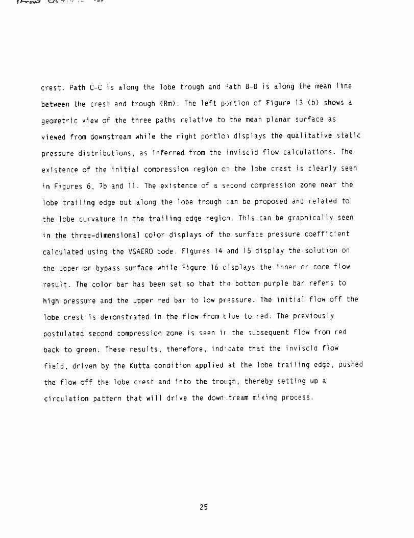
the lobe curvature in the trailing edge regicn. This can be graphically seen

in the three-dimensional color displays of the surface pressure coefficient

calculated using the VSAERO code. Figures 14 and 15 display the solution on

the upper or bypass surface while Figure 16 cisplays the inner or core flow

result. The color bar has been set so that t#,e bottom purple bar refers to

high pressure and the upper red bar to low pressure. The initial flow off the

lobe crest is demonstrated in the flow from t]ue to red. The previously

postulated second compression zone is seen ir the subsequent flow from red

back to green. These results, therefore, indicate that the inviscid flow

field, driven by the Kutta condition applied at the lobe trailing edge, pushed

the flow off the lobe crest and into the trough, thereby setting up a

circu]ation pattern that wi]l drive the down:,tream mixing process.

25

ORIGINAL PAGE IS

OF POOR QUALITY

Cp

-0.7

-0.6

-0.5

-0.4

-0.3

-0.2

-0.1

0.1

0.2

0.3

0.4

Figure 14 VSAERO Display of Pressure Coefficient on Outer Surface of Advanced

High Penetration Mixer

26

-_,-,_._:_'_pAGE IS

OF PoOR QUALIIYCp

-0.7

-0.6

-0.5

I

-0,4

,ii

-0,3

-0.2

-0.1

0.1

0.2

0.3

0.4

Figure 15 VSAERO Display of Pressure Coefficient on Outer Surface of AdvancedHigh Penetration Mixer

27

CRI_Ii'_.ALP_.t_E IS

OF POOR QUALITY

Cp

0

Figure 16 VSAERO Display of Pressure Coefficient on Inner Surface of AdvancedHigh Penetration Mixer

2B

IV. DESCRIPTION OF EXPERIMENT

A. Experimental Arrangement

I. Mixer Lobe Cascade Facility

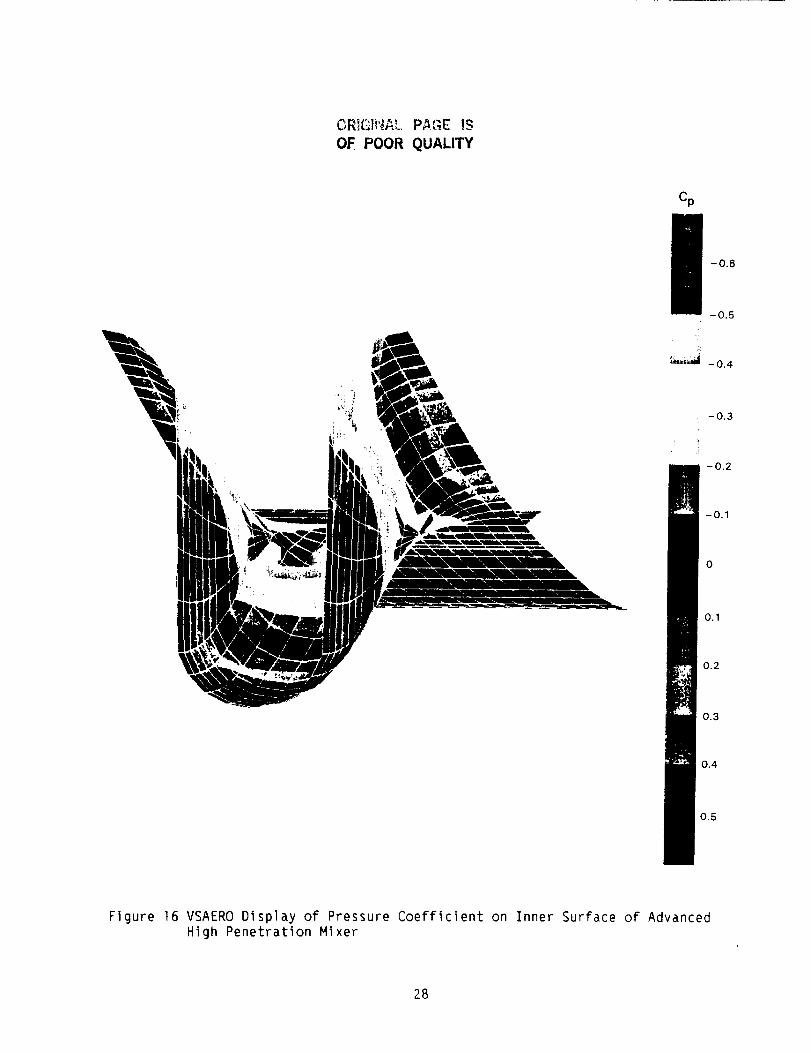
The experiments were conducted in the UTRC Mixer Lobe Cascade Facility shown

schematically in Figure 17. This facility is primarily of pIexiglass

construction, with air circulated by a low pressure/high volume centrifugal

fan. The fan supplies air flow at slightly ab:)ve atmospheric conditions to a

settling chamber containing screens and honeycomb to reduce velocity

nonuniformities. The flow then enters a 5.6 area ratio contraction, passes

through a 20.32 x 21.59 cm (8 x 8.5 in.) rectangular test section, and is

returned by ducting to the fan inlet. Tunnel temperature is equilibrated by

discharging a portion of the fan-warmed air flow from the return ducting and

replacing it with cooler atmospheric air drawn in through a separate fan inlet

port. The settling chamber and connected contraction and test sections are

vibrationally isolated from the rest of the tunnel to enable precise

positional measurements to be made in the test section flow.

All models were stationed a short distance dc_wnstream of the contraction

section. Empty tunnel flow uniformity at this station, as documented by laser

velocimeter measurements was approximately one-quarter percent of U_. Test

section velocity and total temperature were _ominally 37 m/s (120 f/s) and

319°K (575°R) respectively, with both dependent to some degree on atmospheric

conditions.

29

--- DISCHARGE LINEATMOSPHERIC f RETURN LINE

,c--INTAKE _E _ _]

_l.J L_L_ "_'cHAMBER _.= SECT'ON_SECT,ON_.I I Ir-' ,, I I

PROBE -- -- _ LOBED MODEL

W J LVIBRATION/ / PT

/ ,SO_T,ON/ --"HONEYCOMB I'-'4,._,_.- FAN._- M SECTION L..._ SCREEN 'IFT'

Figure 17 UTRC Mixer Lobe Cascade Facility

2. Mixer Lobe Models

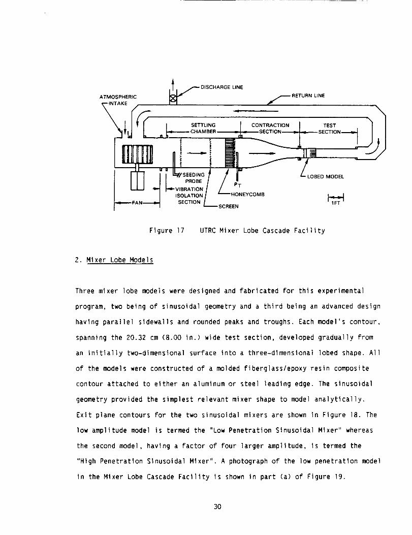
Three mixer lobe models were designed and fabricated For this experimental

program, two being of sinusoidal geometry and a third being an advanced design

having paralle] sidewalls and rounded peaks and troughs. Each model's contour,

spanning the 20.32 cm (8.00 in.) wide test section, developed gradually From

an initially two-dimensional surface into a three-dimensional lobed shape. A11

of the models were constructed of a molded Fiberglass/epoxy resin composite

contour attached to either an aluminum or steel leading edge. The sinusoidal

geometry provided the simplest relevant mixer shape to model analytically.

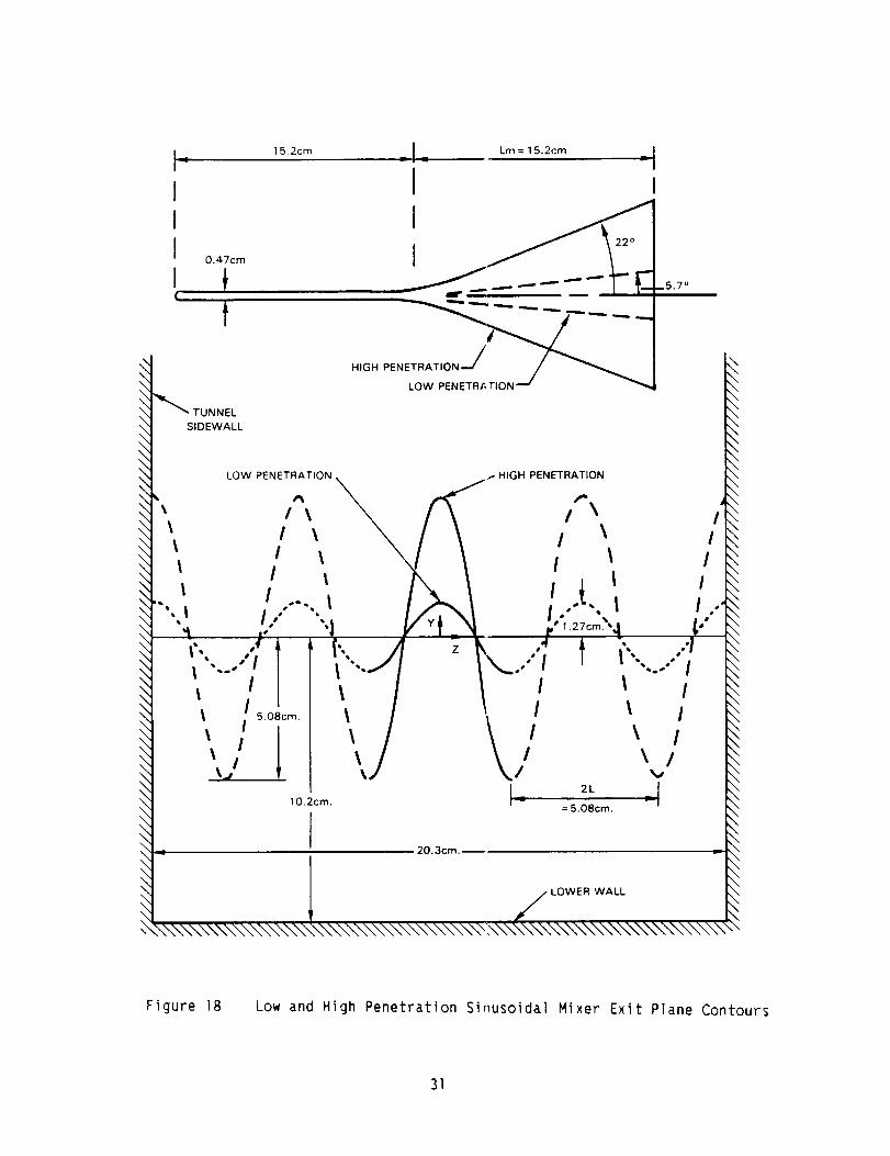
Exit plane contours For the two sinusoidal mixers are shown in Figure 18. The

low amplitude model is termed the "Low Penetration Slnusoidal Mixer" whereas

the second model, having a Factor of Four larger amplitude, is termed the

"High Penetration S1nusoidal Mixer". A photograph of the low penetration model

in the Mixer Lobe Cascade Facility is shown in part (a) of Figure 19.

30

\\\\\\\\\\\\\\\\\\\\\\\\\\\\\

\\

\

\

\

\

\\\\

IIII

0.47cm

I iI

__5.7o

"_'_ TUNNEL

SIDEWALL

HIGH PEN ET(_wA TIpOENNET_R i -TION--" J/___"_

• LOW PENETR/_TION X ,,_,,_,,f.-. HIGH PENETR_,_ON ,

'-.., /..----.,' /Z.,,! ;.--'-.., :..."• Is d' ,, • 1.27cm. ', •,t • 1. p" '_f _x r ,1

,..'..

';......,,'l' t'..-,' z t ,,,,.....;,l I / l I l I

',., I ',l \; "

_\\\\\\\\\\\\\\\"_.

1 _, _l10.2cm. _' = 5.08cm. -- I

20.3cm.

LOWER WALL

,x.\',,,_\\\\\\\\\\\\\\',,b:_\\\\\\\\\\\\\\\\\_

Figure 18 Low and High Penetration SinusoidaI Mixer Exit Plane Contours

31

ORIGINAL PAGE IS

.OF. pOOR QUALITY

(a) LOW PENETRATION SINUSOIDAL PLANAR MIXER

(b) ADVANCED HIGH PENETRATION PLANAR MIXER

Figure 19 Planar Lobed Mixers Installed in the UTRC Wind Tunnel

32

The models transitioned in cross-section fFom a surface that was initially

flat to one that was a sinusoid and whose naximum amplitude steadily increased

with downstream distance. At the exit plane the mean sinusoidal lobe amplitude

for the low penetration mixer was 1.27 cm (0.5 in.) and for the high

penetration mixer 5.08 cm (2.0 in.). Starting from one test section wal] at

maximum amplitude, the contours of both mc,dels reached the opposite wall after

four cycles (5.08 cm. (2.0 in.) wavelengtr) had been completed. Both models

had the same overall length of 25.4 cm. (10 in.) and shared a common forward

section to which their individual molded contours were attached. This forward

section consisted of a 0.47 cm (0.188 in._ thick steel flat plate that was

bracket-mounted to the test section's sid,_ walls. The plate had a rounded

leading edge that was followed a short distance downstream by boundary layer

trips on its upper and lower surfaces. Th_ molded contours were mounted at the

plate's trailing edge by tongue-and-groove attachment, with the trailing

surface of the plate having a 5 degree be_el to make a smooth transition to

the 0.I0 cm (0.04 in.)thick contoured lobe surface. The downstream end of the

model's molded contour was supported at the base of its outer lobes by a pair

of 0.08 cm (0.032 in.) diameter rods mounted to the test section floor.

The third model, referred to as the "Advanced High Penetration Mixer" was

designed to simulate, two-dimensionally, _he flow field of an axisymmetric

mixer lobe configuration for advanced aircraft turbofan engines. In addition

to the mixer lobe contour, it was necess6ry for the model to include

sufficient portions of the engine plug, _,hroud, and the turbine casing wall

separating the primary and fan f]ows in order for f]ow through the lobes to be

properly simulated. Therefore, the model consisted of three main components:

33

the lobe body, shroud, and plug. Each of these components spanned the test

section and were secured to the tunnel surfaces to maintain their correct

relative spacings. The exit plane contour and cross-section for this model

shown in Figure 19<b) and Figure 20 is a photograph of the model installed in

the lobe cascade facility. The model had the same 5.08 cm. wavelength as the

sinusoidal lobes but had parallel sidewalls capped by half circles. Relative

to the upstream flat plate centerline (y:O), the lobes were unsymmetrical in

that the exit plane height of the upwardly directed lobe was 2.94 cm. (lobe

interior dimension) and that of the downwardly directed lobe, 3.10 cm. The

peak-to-peak amplitude of the mixer was therefore 6.04 cm., intermediate

between the 2.54 cm. and 10.16 peak-to-peak amplitudes of the two sinusoidal

models. In addition to having differing amplitude up and down lobes, the slope

of the lobe peaks in the axial direction differed. As discussed relative to

the transverse velocity components subsequently, the bottom lobe sloped at a

steeper angle. Also, the trailing edge region of the upper lobe tapered to a

shallow angle.

The lobe body was made up of an aluminum forebody and an attached

fiberglass/epoxy resin composite contour, with an overall length of 56.24 cm

(22.14 in.). Leading edge shape of the forebody was that of a 4-to-I ellipse.

This shape was blended smoothly with the attached fiberglass/epoxy resin

composite contour, which modeled the two-dimensional primary and fan flow

walls and transitioned into a three-dimensional lobed surface. The

two-dimensional forward portion of the model was bolted to the test section

sidewalls, while the rear of the model was supported by a pair of spacers

attached to the plug surface and lobe trailing edge. Seams formed by the

adjoining model and test section sidewalls were sealed by a fillet of silicon

adhesive in order to isolate upper and lower surfaces of the model.

34

Flow

I _ _ .J;I_ 32.1cm Lm 24 lcrn

I

iL.- INNER WALL

C OUTER WALL

TUNNEL

SIDEWALL

-"3,

(AI AXIAL CROSS-EL:CTION

Y SIMULATED

_\\\\\\"__\\\'\_\\_'-,,\',,__'-,,\\\\\\\\\\\_

_\\\\\\\\\\\\\\\\\_:,%,\\\\\\\\\",_.',,(.; _ 20 3crn --

,B) EXIT CONTOU, q

_m 4 03cm

,Ocm 3 75cm

¢

_ SIMULATED

PLUG

Figure 20 Advanced High Penetration Hixer Section and Exit Plane Contour

The shroud and plug surfaces were each formed by a pair of 0.95 cm (0.375 in.)

thick contoured aluminum rails supporting a 0.32 cm (0.125 in.) thick

plexiglass sheet across the test section wi:Jth. Each of the rails had one edge

flattened for bolting to the test section c_iling or floor, while the other

edge was machined so that the attached plexiglass sheet would assume the

appropriate axial surface contour at the ccrrect relative spacing from the

lobe body. The shroud and plug surfaces extended upstream to the test section

35

inlet so as to provide un,iform flow to the model, with the remaining test

section inlet flow diverted beneath these surfaces. Downstream of the lobe

body the shroud and plug contours were extended as straight wails for a

distance of some four times their wall spacing. The straight wails were

approximately parallel, being set at a slight relative angle to account for

wail boundary layer growth and thereby maintain a constant pressure condition

downstream of the lobe model.

B. Instrumentation

Quantitative measurements made during the experimental tests included Laser

Doppler Velocimetry (LDV), flow total pressures, wall static pressures, inlet

boundary layer documentation and positional information. Qualitative

understanding of the flowfield was also obtained by means of surface oil flow

visualization.

I. Laser Doppler Velocimetry

A commercially available 2W argon-ion laser system was used for making flow

velocity measurements in the tunnel test section, with the laser system

mounted on a manually controlled three-axis traverse table and interfaced with

a computer for data processing and storage. The system, similar to that

employed in the previous mixer nozzle study (Reference 4) was configured in a

dual beam ("fringe") mode using 0.5145 micron wavelength light, with

collecting optics typically positioned for forward scatter. By means of

heterodyne detection of the Doppler shift in the light collected from the

36

intersection of incident beams during seed particle passage, instantaneous

flow velocity was obtained For that component w,lich was in the plane of and

perpendicular to the bisector of the incident beams. Bragg shifting was used

to eliminate directional ambiguity. Axial and s:)anwise velocity components

were taken by passage of the light beam through the test section's glass

sidewalls, while the vertical velocity component was measured by reflecting

the beams down through a glass window mounted in the test ceiling and

operating the laser system in a back-scatter mode.

Flow seeding for the sinusoidal lobe tests was 0y means of aluminum oxide

particles having a nominal diameter of 0.3 micron, which were fluidized in a

low pressure seeder and injected into the closed loop tunnel downstream of the

test section. Seeding for the advanced model t_st was accomDlished by atomizing

corn oil, having a nominal diameter of 1.0 micron, and injecting it into the

flow upstream of the settling chamber through a seeder probe designed to

minimize flow disturbance.

The collection optics signal was sent to a courter-type signal processor.

Operated in its continuous mode, the processor measured the time for a

particle to cross 8 fringes and then transferr_:_d this information to the

computer. Typically, I000 such measurements were taken per data point in order

to calculate a mean value and standard deviati<:,n of the velocity component.

Data point locations were established based on choosing a point on the model

as a coordinate origin and recording relative distances from this origin as

provided by calibrated potentiometer outputs o_ the laser system traverse

table.

37

2. Total and Static Pressures

Total pressure measurements made during this test program included detailed

planar surveys downstream of each model, boundary layer traverses at selected

model locations, and continuous tunnel operation monitoring. Total pressure in

all cases was sensed by a dedicated transducer whose calibration was checked

prior to and Following each test run. Types of probes used included a kiel

head probe for the planer surveys and a Flattened impact probe For the

boundary layer traverses. The probe support exited the test section through a

sidewall slot and was mounted to and moved by a computer controlled two-axis

traversing unit. Tunnel total pressure was measured with a pitot-static probe

mounted in the upstream end of the test section floor during the sinusoidal

lobe tests and with a kiel probe located downstream of the last flow

straightening screen in the settling chamber for the advanced mixer tests.

During the sinusoidal lobe tests, the test section static pressure was

obtained with a floor mounted pitot-static probe in the upstream end of the

test section. In addition, the common forward section of the two sinusoidal

lobe models had a pair of static taps on both upper and lower surfaces to

assist in aligning the model with the incoming stream. For the advanced

penetration model tests, forty-six static pressure taps were provided at

locations distributed over the model surface and wind tunnel walls.

38

3. Flow Visualization

A variety of standard flow visualization techniques were applied to gain

understanding of the flow about the lobe models. These included tuft and smoke

motion and oil film surface patterns. Fluorescing dye was mixed with the oil

prior to surface application in order improve _:urface pattern clarity.

4. Boundary Layer Definition

Hot wire anemometry was employed to define the boundary layer approaching the

lobe region of the models. Surveys were taken ()n the upper and lower surfaces

in the leading edge region.

5. Experimental Technique

Test preparation involved installation of a moJel in the tunnel test section,

calibration of measurement equipment, and preliminary measurements in the

flowfield to verify correct model placement. The sinusoidal models were

initially positioned to be aligned with the tunnel centerline horizontal

plane. Preliminary tests were then performed, Dy measuring static pressures

via taps in the models' common forward section, and the model's pitch angle

adjusted, if necessary, to achieve a proper zero flow angle alignment. In the

case of the advanced penetration model, its three components were designed to

maintain fixed relative spacings, with the entire assembly mounted horizontally

39

in the test section such that the tunnel centerline bisected the initial lobe

station. A preliminary test was similarly performed for this model by sampling

all static pressure tap locations to insure that proper component alignment

and spacing had been met. All model edges in contact with the test section

sidewalls were sealed to prevent leakage between upper and lower surfaces.

Equipment preparation primarily involved the laser system, including alignment

of the laser table, adjustment of the laser optics, activation of the data

acquisition software, locating the positional origin of the model, and fine

tuning the signal processor and seeding supply to obtain a satisfactory

signal-to-noise ratio and data rate. A double check was made to verify that

the LDV measured velocity values were correct. The first consisted of

determining the velocity at a given radius on a wheel rotating at a constant

rate with the LDV and comparing that result with the algebraically computed

value. The second method was to compare the LDV measured velocity at a point

in the test section flow with the value computed from a pitot-static probe

measurement at the same point. Good agreement was realized with both methods.

For test runs in which a total pressure survey or boundary layer traverse was

to be taken, preparation included alignment of the traverse mechanism,

locating the positional origin, and check-out of the computer controlled

traverse unit, data acquisition software, and pressure transducer calibration.

4O

Prior to taking data, the tunnel was operated For a sufficient length of time

to produce quasi-equilibrium test section con0itions. Following this, the

barometric pressure, laser optics information, and signal conditioner settings

were recorded and a final correction made in the positional origin to account

for tunnel growth.

The test procedure for acquiring LDV data was to record the barometric

pressure, laser optics information, and signal conditioner settings into the

computer, then position the probe volume at either the maximum or minimum of

the Y-axis survey plane, activate the seeding system, execute the LDV data

acquisition program to acquire lO00 valid sam[,les of the velocity component at

that location, stop the seeding system, revie_._the velocity histogram

following completion of the on-line processinc: to insure that the data point

is acceptable, instruct the computer to store this result along with the test

section total pressure and total temperature, and finally manually control

probe volume movement to the next Y-axis loca_ion. The seeding system was

again started, and the same acquisition steps repeated until a complete

vertical (Y-axis) traverse of approximately 3(i_different point locations had

been acquired. This resulting collection of d_,.tapoints was designated as a

'run'. The laser probe volume would then be moved to the next spanwise

(Z-axis) position and the entire procedure re_}eated until traverses at

required spanwise locations had been completed. These steps were again

repeated twice more to obtain the remaining t'_o components of velocity.

4l

Acquisition of total pressure survey data was facilitated by computer control

of both probe movementand data acquisition and reduction. After having

manually positioned the total probe at a starting location in the survey grid,

the computer software programwas initiated to samplethe probe pressure and

test section pressure and temperature, computeand output test parameters,

store the data, movethe probe to the next designated grid location, and

repeat these steps until array completion. Boundary layer traverse data was

obtained in a similar manner, but with manual control of probe movementbased

on operator selection of appropriate traverse data point locations.

Flow visualization tests were performed by forming a solution of medium-weight

gear oil and a florescent pigment, applying this mixture as small dots

randomly spaced on the model surface, operating the tunnel for a period

sufficient to allow the dots to spread and thin under the action of

aerodynamic forces, opening the test section, and photographing the patterns

under ultra-violet illumination.

6. Data Analysis

Data reduction was performed by on-line computers for this test program, with

a mini-computer used for the LDV and a personal computer (PC) for the total

pressure measurements. Software programs were written for each to meet

specific test requirements.

42

For the LDVtest phase, data was sent to the computer via the signal

processor. The processor transmitted a number identifying the amountof time

taken for a flow seed particle to travel a knowndistance through the laser

probe volume. From previously input parameter constants related to the laser

optics, geometric alignment, and beamproperties, the program could compute

this distance and hence a flow velocity. In crder to achieve an accurate

velocity measurement,lO00 samples were taker and stored for each point

location. The program calculated a velocity value for each sampleand computed

a meanand variance of the sample population A histogram was generated by

dividing the total range of possible velocities, as determined by the filter

settings of the signal processor, into 100 e(lual ranges or 'bins' and then

assigning each of the sample velocities to i_::sappropriate bin. The bin

containing the most samples was located by ti_e program, adjacent bins above

and below this central bin sequentially test_d until sampleless bins were

found, and a meanand variance computedfor this resulting sample subset. The

operator could choose a subset of this reduced population, if upon examining

the histogram it was found that the distribution was skewedappreciably from

the expected Gaussian distribution. In that case, a meanand variance would be

computedfor this new subset. The meanand variance was stored along with

probe location and tunnel condition information for each data point.

Model reference velocity, U_ , was computedFrom Bernoulli's equation, using

the test section pitot-static probe pressures for the sinusoidal lobe models

and the test section total pressure together with an average of the plug and

shroud upstream static tap pressures for the_ advancedpenetration model.

43

The total pressure survey data was processed by calculating a normalized total

pressure for each of the survey data points. Boundary layer calculations were

based on the assumption of constant static pressure across the layer.

V. RESULTS AND DISCUSSION

A. Experimental Observations

I. Data Presentation

This section of the report presents three-dimensional mean velocity and total

pressure measurements acquired just downstream of the mixer lobe exit plane

for the three mixer configurations considered in this study: Model l- Low

Penetration Sinusoidal Mixer, Model 2 - High Penetration Sinusoidal Mixer and

Model 3 - Advanced High Penetration Mixer Geometrical characteristics of

these three mixer configurations are described in the section, "Description of

the Experiment".

Data are presented at a location downstream of the trailing edge,

7 = x - XTE, as a function of spanwise (lateral) position, z, and transverse

position, y. The coordinate system was previously shown in the sketch on page

9. These coordinates represent physical values normalized by the lobe

half-wavelength of L = 2.54 cm. All other lengths such as boundary layer

parameters are presented in this normalized format. Tables D.l.l-3, D.2.1-3

and D.3.1-3 provide Laser Doppler Velocimetry (LDV) measured axial, transverse

44

and spanwise mean velocity components (U_+u,_,w) for the three

configurations, respectively. Tables D.I.4 and D.2.4 present exit station

total pressure measurements for the sinusoida mixers in terms of a normalized

total pressure, P-_. As defined in the List of Symbols, P_ represents the

measured total pressure referenced to the upstream reference static pressure,

p_ and normalized by the reference dynamic pressure, q_ . Table D.3.4

presents total pressure results for the advanced mixer in terms of the ratio

of measured to upstream total pressure. The f:}11owing discussion of results

begins with the Model 1 low penetration mixer and proceeds through the

remaining two models.

The axial component is given as a fraction of the upstream reference velocity,

U_ . Secondary flow components v and w are presented in a non-dimensional form

with the upstream reference velocity, U_ , as the normalizing quantity.

2. General Observations

Axial velocity and total pressure measurements at the exit plane of the two

sinusoidal waveform mixers indicated significant viscous retardation effects

occurred within the lobe region. Low momentu_ fluid tended to be concentrated

in the peak region within the lobe interior. %imilar measurements acquired

with the advanced high penetration mixer showed much thinner lobe boundary

layers with inviscid flow extending well intc the rounded lobe peak region.

45

Transverse velocity measurementsat the exit plane of all three models showed

significant cross-stream flows on the order of I0 to 30 percent of the lobe

exit axial velocity. Magnitudes were largest for the high penetration

sinusoidal model which also had the largest lobe amplitude (or equivalently,

largest rampangle). Transverse velocity magnitudes diminished in the interior

lobe peak region of the sinusoidal modelswhereas the advancedmixer displayed

near ideal velocity levels well into the lobe peak.

Spanwisevelocity componentmagnitudes at the lobe exit plane were

substantially smaller than the transverse componentfor all three models. The

combinedtransverse - spanwise secondary flowfield was characterized by two

counter-rotating axial vortices located within each spanwise wavelength of the

periodic models. The circulation associated with each axial vortex was Found

to be dominated by the contribution from the transverse velocity field.

Surface flow visualization of the lobes showedskewingof the near surface

flow toward the lobe peak and trough regions. The degree of skewing was

greatest for the two high penetration models. The direction of lateral

boundary layer fluid migration was in agreementwith the direction of lateral

pressure gradients predicted by the analyses.

3. Mixer Lobe Flow Visualization

Surface flow visualization patterns for all three models considered in this

study were qualitatively similar and in agreement with expectations based on

the analytically predicted lobe surface pressure distributions given in

46

Section III and shown schematically in Figure 13. These distributions are

reviewed briefly here. As shown in Figure 6, both sinusoidal mixers display an

initial pressure rise (dp/dx) along the crest line (z=O), followed by a

maximum and decline back to freestream pressure. The pressure distributions

are similar, as would be expected for geometrically similar designs, but four

times larger for the high penetration model because of the amplitude ratio of

four. The trough line (z=l) distribution is sin, ilar but of opposite sign and

the mid-lobe position (z:.5) shows no deviatioF from freestream static

pressure. As shown by the contours, a pressure ,_radient (dp/dz) exists from

crest-to-trough and is a maximum at an axial p(,sition midway through in the

lobe and between z=.25 and .75. This spanwise Tegion coincides with the region

of steepest spanwise slope of the cosine function describing the contour

(y = h cos_ z).

A photograph of the two sinusoidal mixer modeli is provided in Figure 21.

Surface flow visualization for the low penetration model displayed a weak

spanwise flow from crest to trough in response to the above described pressure

gradient. Surface flow visualization for the high penetration model, given in

Figure 22, was much more dramatic, displaying _ downwardly skewed near surface

flow from crest to trough. This surface flow i_;particularly evident midway

through the model on the steep sides of the lo0e, as expected based on the

above. Also evident is skewing of the approach boundary layer at the entrance

to the lobe region. Surface streaks aligned with a trough (z=1) run directly

aft down the trough centerline. Streaks aligned between trough and crest (z=O)

are rapidly turned laterally toward trough centerline. These results indicate

47

LOW PENETRATION HIGH PENETRATION

Figure 21 Sinusoidal Mixer Models

TRAILIN(EDGE

APPROACHFLOW

Figure 22 Flow Visualization Study of Surface Streamline Pattern on HighPenetration Planar Mixer

48 OF POOff QUALITY

that the low momentum boundary layer fluid apl,roaching the model should gather

in the trough thereby producing blockage in the bottom OF the trough at mixer

exit. This blockage is confirmed later when axial velocity and total pressure

data are examined.

Analytical predictions of pressure distributi,)ns for the advanced mixer are

shown in Figures II and 12 and in Figures ]4-16. For this discussion we shall

concentrate on flow patterns as viewed from t!_e top of the mode] For which the

crest pressure distribution is given by the Figure II curve labeled "external

flow". The curve displays a rapid rise (flow Jeceleration) at Station 56

which is the beginning of the lobe region. This is followed by a decline

(acceleration) to Station 64 and final return to freestream static pressure at

mixer exit, Station 66. The trough pressure distribution is given by the

Figure 12 curve labeled "internal flow". The curve displays the same character

as the crest distribution except magnitudes are lower. The net effect, when

the curves are overlaid, is that a pressure gradient from crest to trough

exists over the length of the model except fc,r a weak gradient from trough to

crest near the trailing edge. The maximum gradient exists at the lobe entrance

(Station 56). The above described pressure pattern is sketched in Figure 13.

Advanced penetration model flow visualizatior shown in Figure 23 displays the

spanwise skewing from crest to trough expectE_d based on the above pressure

distributions. Particularly evident is the s_rong curvature of surface traces

on the lobe crest midway through the mixer. C,ne would infer From these

pictures that significant thinning of the cr(_,stboundary layer would occur at

the expense of trough boundary layer thicken rig.As discussed below, boundary

layer measurements obtained at mixer exit confirmed these expectations.

_9

TRAILING APPROACH

EDGE- FLOW

Figure 23 Flow Visualization Study of Surface Streamline Pattern onAdvanced High Penetration Mixer

In summary, flow visualization studies showed strong three-dimensional

boundary layer effects for the high penetration mixer models as a result of

the lobe-induced surface pressure field. The process of boundary layer growth

under varying streamwise pressure gradients and spanwise skewing by virtue of

varying spanwise pressure gradients requires the use of computational

procedures to establish exit plane characteristics. As will be shown,

prediction of exit plane displacement thickness distributions is needed to

obtain accurate estimates of the circulation and vorticity field shed from

mixer trailing edge.

50

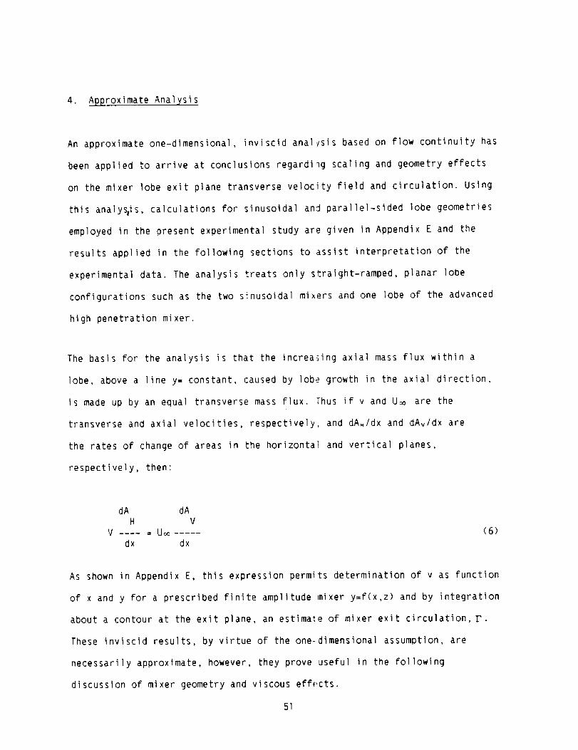
4. Approximate Analysis

An approximate one-dimensional, inviscid anal:isis based on flow continuity has

been applied to arrive at conclusions regardiqg scaling and geometry effects

on the mixer lobe exit plane transverse velocity field and circulation. Using

this analysris, calculations for sinusoidal and parallel-sided lobe geometries

employed in the present experimental study are given in Appendix E and the

results applied in the following sections to assist interpretation of the

experimental data. The analysis treats only s_raight-ramped, planar lobe

configurations such as the two sinusoidal mixers and one lobe of the advanced

high penetration mixer.

The basis for the analysis is that the increa_ing axial mass flux within a

lobe, above a line y= constant, caused by lobe growth in the axial direction,

is made up by an equal transverse mass flux. Fhus if v and U_ are the

transverse and axial velocities, respectively, and dA./dx and dAv/dx are

the rates of change of areas in the horizontal and vertical planes,

respectively, then:

dA dAH V

V = Uoo ..... (6)dx dx

As shown in Appendix E, this expression permits determination of v as function

of x and y for a prescribed finite amplitude mixer y=f(x,z) and by integration

about a contour at the exit p]ane, an estima1:e of mixer exit circulation, F.

These inviscid results, by virtue of the one-dimensional assumption, are

necessarily approximate, however, they prove useful in the following

discussion of mixer geometry and viscous effects.

51

5. Low Penetration Sinusoidal Mixer

Approach Boundary Layer Documentation - Hot wire anemometry was employed to

define the characteristics of the boundary layer approaching the lobe region

of the test model. E survey was taken in the transverse direction on tunnel

centerline at an axial position 4.33 from the leading edge of the model, fhis

position corresponds to the transition location between the upstream flat

plate approach section and the downstream three-dimensional contoured lobe

region. Measured boundary layer characteristics (Table D.4) at this location

(normalized by 2.54 cm) were: displacement thickness, 6* = 0.024, momentum

thickness, 8 = 0.017, 99% boundary layer thickness, 6 = 0.145, and shape

factor, H = 1.41. The measured boundary layer thickness of 0.145 was close to

the value of 0.127 calculated for a'zero pressure gradient turbulent boundary

layer growing from the plate leading edge.

The measured shape factor was in good agreement (approximately 3% lower) with

the value which applies to zero pressure gradient boundary layers at the test

momentum thickness Reynolds number of Re e = 970 (Reference 15) From these

measurements it is concluded that normal turbulent boundary layer flow

approach conditions were obtained.

Axial Velocity Field - At the mixer exit station located just downstream of

the mixer trailing edge (7 = 0.36), the velocity field is categorized by

regions of inviscid (near reference velocity) flow and viscously affected

(retarded) flow. As shown in the contour plot of Figure 24, inviscid flow

exists at distances removed from the lobe exit surface and retarded flow

52

occurs near the outside lobe surface and within the bulk of the interior

portion of the lobe peak. Specifically, the U/U,: = 0.99 contour demonstrates

that measureable viscous retardation effects within the lobe extend from the

lobe peak (z = O, y = 0.5) to the mixer centerl ne (y = 0).

0

-025 1

-0_)

-OPS

-IC0

l I l J I l l i-075 -050 -02S 0 ,2_ 050 0 75 I CO

SPANWISE DISTANCE Z

Figure 24 Contour Plot of Axial Velocity Field at Trailing Edge of LowPenetration Sinusoidal Mixer

More specifically, Table D.4 shows that within the interior of the lobe, _*

and 6 were 0.087 and 0.48, respectively, as measured along the line z = 0

relative to the lobe peak (y = 0.5). The 6" measurement can be interpreted as

a blockage in the lobe interfor peak region which effectively reduced the

nominal (geometric) lobe penetration from 0.5 tc 0.41, or to 83Z of its

nominal value. The deleterious effect of this blockage on transverse velocity

component magnitude is discussed subsequently.

53

As indicated by Table D.4, the boundary layer in the outer flow above the lobe

peak along the samez = 0 line wasapproximately a factor of three smaller

than that measured within the lobe (6= 0.15 as opposed to6= 0.481. This

significantly lower value is consistent with the previous discussion of flow

visualization results and lateral pressure gradients. In the outer flow, the

boundary lay@r along the peak surface is driven sideways and downward toward

the trough by the imposed inviscid pressure gradient field and consequently

thinned. The opposite effect occurs within the lobe interior where pressure

gradients cause boundary layer fluid migration toward the peak region. Viscous

retardation in the peak region is further aggravated by the narrowing of the

sinusoidal lobe waveform with increased distance, y. Fluid migration and peak

narrowing cause merging of the viscous layers from both sides of the lobe on

the lobe centerline (z = 01. The following section presents related exit plane

total pressure results.

Total Pressure Field - Normalized total pressure contours given in Figure 25

confirm the previously presented axial velocity results regarding the

existence of significant viscous effects within the interior of the lobe and

near the lobe surface. Using the 0.99 contour as an indicator of the dividing

line between inviscid and viscous regions, it is seen that viscous effects

extend throughout the region bounded by the lobe surface and the mixer

centerline (y = 0). Low total pressures in the peak of the lobe indicate that

viscous effects dominate this region, thereby contributing to blockage.

In summary, both axia) ve)ocity component and total pressure data indicate

significant viscous retardation effects for this model. Subsequent sections

will discuss implications of these findings relative to the magnitude of the

transverse velocity component, lobe exit plane circulation and preferred mixer

lobe geometries.54

C3

_Pu_

c-

.I

Spanwise Distance z

Normal i zedTotal Pressure

1 8.2000

2 0.4000

3 0. G088

4 0.8000

5 0.9900

Figure 25 Contour Plot of Normalized Total Pr=_ssure Field at Lobe TrailingEdge of Low Penetration Lobed Mixer

55

Transverse Velocity Field - At the mixer exit station the transverse velocity

component data indicate a general cross-stream (vertical) flow as would be

anticipated in response to the vertical penetration of the lobe contour into

the stream. Considering the symmetrical lobe segment extending from z = 0 to

z : .5, velocities are upward within the interior of the lobe (y < 0.5 cos_z)

and generally downward outside the lobe (y > 0.5 cos _z). As shown in the

contour plot of Figure 26 and Table D.I.2, the greatest transverse velocity

components (those in the range from 7 to 8.7% of Um) are directed upward and

occur within the upper half (y Z O) of the interior of the lobe. Values of

this magnitude extend across the lobe (from z : 0 to z : .4) with lower values

obtained near the lobe surface at all values of z. Contained within this

contour is a smaller region in the central portion of the half-lobe where

maximum values in the range from 8 to 8.7% of U_ are obtained. Outside these

contours, values decay to negligible levels as distance from the lobe surface

increases.

Examination of the transverse velocity component magnitude variation with y

provides insight into overall lobe flowfield development and for this purpose

the z = O line centered on the lobe peak has been selected. As shown in Figure

27, a maximum value for v of 8.5 % U_ is obtained inside the peak at a y

value of 0.3. Values decrease gradually with increasing distance from the lobe

peak with finite values of several percent obtained below the mixer (y < 0.5).

The rate of decay of the component in the opposite direction (y > 0.3) is much

more rapid with near zero values achieved at y > 0.6.

56

QJUc--to

or--

_=

tO

1.5 I I I I

/0.5

-0.5

Transverse

Velocity (v/U_)

I -.8000E-81

2 -.GOOOE-O1

3 -.4000E-01

4 -.2000E-01

5 .0000

G .2000E-91

7 .4000E-01

8 .GOOOE-O1

9 .8000E-OI

-1.5 I ! I I-I.0 -.6 -.2 .2 .6 1.

Spanwise Distance z

Figure 26 Contour Plot of Transverse Velocity Field at Trailing Edge of LowPenetration Lobed Mixer

57

2.0

DATA POSITION (z)

C) 0.0

-'_ 1.0 (SHIFTED)

OUTSIDE

LOBE PEAK

INSIDEI

IIIIIIIII

! I 1 I I

0 2.0 4.0 6.0 8.0 10.0

TRANSVERSE VELOCITY AS PERCENT OF Uco

IDEAL

MAGNITUDE

10%

Figure 27 Low Penetration Mixer, Transverse Velocity Component (v/Uo_ x 100)

58

Also shown in Figure 27 is the degree of sym_etry achieved in the experiment.

Circular and triangular symbols show results obtained at z = 0 and z = l,

respectively. The z=l velocity and position data have been changed in sign to

permit them to be overlaid onto the z:O data For this symmetrical model, data

at these two locations should be identical.-his symmetry is observed to be

true within the error band estimated to be 1:_ssthan one Dercent of the

reference velocity. Of particular importance is that the vertical component

did not achieve its ideal maximum value base:_ on lobe geometry. For an

inviscid flow and straight-ramped lobes such as considered here, the velocity

vector at the lobe peak should be parallel t) ramp slope. Based on the lobe

peak ramp angle (turning angle) of E= 5.7° and an axial velocity equal to the

upstream reference velocity, U_, the ideal ::ransverse component magnitude at

the mixer exit should be U_ tanE or 0.1U_ As a percentage of this ideal

value, the maximum magnitude achieved was only 85%. This degradation is

attributed to boundary layer blockage in the lobe peak region which

effectively reduced lobe penetration. It is important to note that this value

of 85% is in close agreement with the 83% effective lobe penetration

calculated in the previous section from bounJary layer displacement thickness.

Other comparisons to inviscid behavior can be made. Following the calculation

procedure described in the above section, "#pproximate Analysis", it is shown

in Appendix E that transverse velocity magnitude should be given by:

_/ 2l- (y/h)

v = U tan _ ........... (6)

arc cos (y/h)

59

where h is the sinusoidal amplitude <one-half peak-to-peak), or 0.5 for the

low penetration model. This relation is shownas a dashed line in Figure 27

and as not@dabove, the maximumvalue of 0.I U_is not achieved at y = 0.5.

The predicted decay with increasing distance from the lobe peak is observed in

the data, but contrary to analysis, non-zero componentsare measuredat values

of y less than 0.5.

In summary,the transverse velocity componentmeasurementsfor the low

penetration sinusoidal mixer follow overall expected trends basedon inviscid

analysis. Maximumvalues, however, are only 85%of ideal and this is

at&ributed to blockage in the lobe peak region caused by boundary layer

convection and growth within the lobes.

Spanwise Velocity Field - As in the case of the transverse component, the

spanwise velocity field at the mixer exit station displays cross-stream

motions in response to the penetration of the lobe contour into the stream. In

contrast with the transverse components, the spanwise component magnitudes are

small, reaching values of only several percent U_ in the vicinity of the lobe

surface. This general behavior is displayed in Figure 28 where spanwise

component vectors are plotted in terms of percent U_. Near zero values are

obtained along the line z = 0 as expected based on symmetry arguments.

It can be inferred that the variation of spanwise component magnitude with y,

exterior to the lobe and in the vicinity of the lobe surface, is such that the

vector sum of w and v is parallel to the surface tangent. This tangency

condition is consistent with the data which shows maximum values outside the

lobe peak and decreasing values toward mixer centerline. In summary, spanwise

6O

OR|r.._iAL I'AGE !S

QE -POOR QUALITY

O6

0 6 12 16 1.5 %4 13 1.1 _8

>-.

Z

0 0.4

2

mr

Z< 0.2

12 23 2_3 21 19 16 13 10

o--';--_,T7

0

0

1

O

IO

2.7 3.0 23 2.0 15 13 8

1 ..,=..._____-4 2.3 _2"5 _2"0 1.5 1. I 8

- , -4 6_ 1.7 1.8 i _

_.._ -7-- 4 - - 12 3

1 -1 6 2

1 5 lll 12 |%,0_" 12 11 5I I I I I 1

02 04 06 08

SPANWISEPOSllON. Z

6

8

77

5

1

Figure 28 Low Penetration Mixer, Spanwise Velocity Field (w/U= x I00)

velocity measurements indicate that while Maximum values can reach levels as

high as 34% of the maximum transverse component level, this component of the

secondary flow vector field is generally much weaker than the transverse

component.

Combined Transverse-Spanwise Velocity Fiell - Figure 29 is a vector plot of

the low penetration model lobe exit secondary velocity field measured at a

position just downstream (7 = 0.36) of the lobe trailing edge. The existence

of two counter-rotating axial vortices wit2in the single lobe segment is

clearly evident. The much higher dens%ty oF measurements and greater

measurement accuracy provide a much improved definition of the lobe-induced

circulations relative to the previous mixer study conducted by Paterson

(Reference 4), using LDV techniques. The circulation associated with these

vortices will be presented in the section, "Circulation Calculations"

61

-1.01,0

Figure 29 Low Penetration Sinusoidal Mixer Exit Plane Secondary VelocityField

6. High Penetration Sinusoidal Mixer

Approach Boundary Layer Documentation - Hot wire anemometry was used to define

the characteristics of the boundary layer approaching the lobe region of the

model. The survey was taken at the same location as that used for the low

penetration model, i.e. 4.33 from the leading edge at the junction of the flat

plate and lobe regions. Measured boundary layer characteristics at this

location are given in Table D.4 and are observed to be about 60% larger than

those obtained with the low penetration model. This difference is attributed

to a thicker turbulent trip in the leading edge region. The shape factor of

1.39 is reasonable being within 4% of the zero pressure gradient value for

this momentum Reynolds number (Reference 15). When compared to the factor of

62

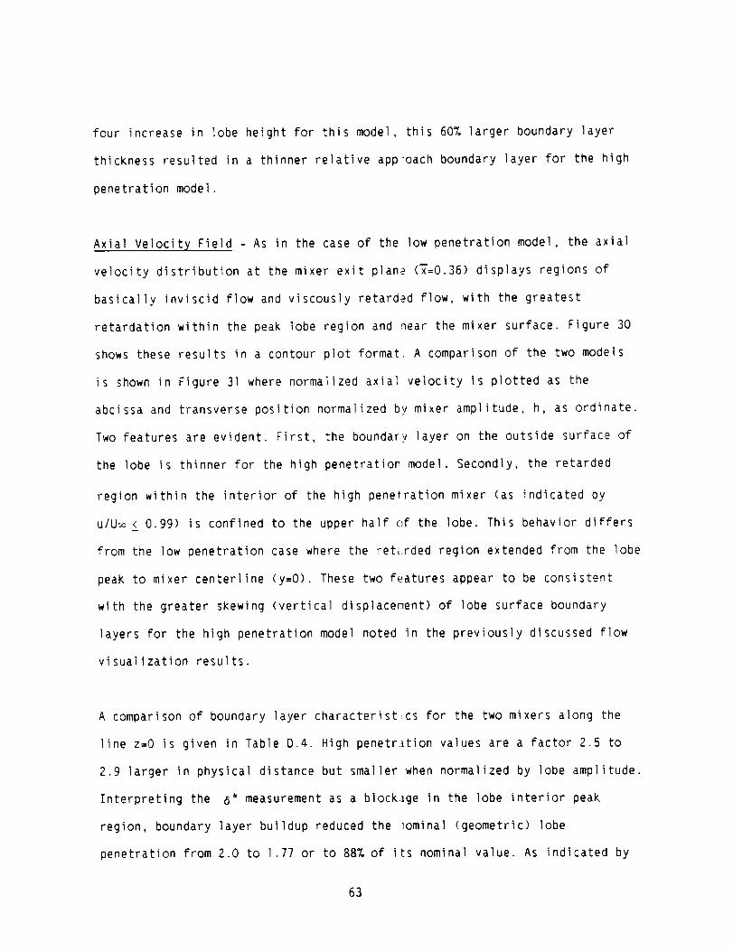
four increase in lobe height for this model, this 60% larger boundary layer

thickness resulted in a thinner relative app,oach boundary layer for the high

penetration model.

Axial Velocity Field - As in the case of the low penetration model, the axial

velocity distribution at the mixer exit plane (T=0.36) displays regions of

basically inviscid flow and viscously retarded flow, with the greatest

retardation within the peak lobe region and near the mixer surface. Figure 30

shows these results in a contour plot format. A comparison of the two models

is shown in Figure 31 where normalized axial velocity is plotted as the

abcissa and transverse position normalized by mixer amplitude, h, as ordinate.

Two features are evident. First, the boundary layer on the outside surface of

the lobe is thinner for the high penetration model. Secondly, the retarded

region within the interior of the high penetration mixer (as indicated by

u/U_ < 0.99) is confined to the upper half (>f the lobe. This behavior differs

from the low penetration case where the ret_rded region extended from the lobe

peak to mixer centerline (y=O). These two features appear to be consistent

with the greater skewing (vertical displacement) of lobe surface boundary

layers for the high penetration model noted in the previously discussed flow

visualization results.

A comparison of boundary layer characteristics for the two mixers along the

line z=O is given in Table D.4. High penetr_tion values are a factor 2.5 to

2.9 larger in physical distance but smaller when normalized by lobe amplitude.

Interpreting the 6* measurement as a block_ge in the lobe interior peak

region, boundary layer buildup reduced the nominal (geometric) lobe

penetration from 2.0 to 1.77 or to 88% of its nominal value. As indicated by

63

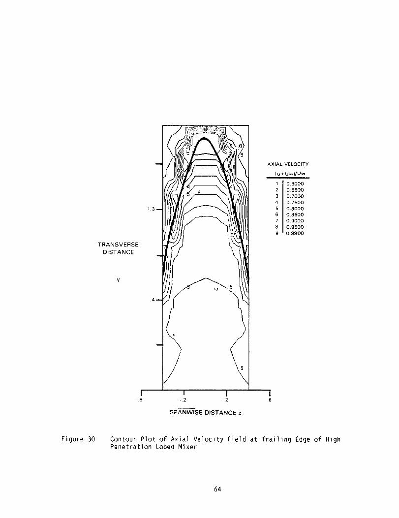
TRANSVERSE

DISTANCE

I f _,iiif-_ I_i_\__ I

d(il!( !l IvVJil ?l;i'!L

I f

.4

I !-,6 -.2 .2 .6

AXIAL VELOCITY

(u + U_)/U:-i

1 0.60002 0.65003 0.70004 0.75005 0.80006 0.85007 0.90008 0.9500

9 0.9900

SPANWlSE DISTANCE z

Figure 30 Contour Plot of Axial Velocity Field at Trailing Edge of HighPenetration Lobed Mixer

64

1.2

1.0

0.8

t---- 0.6

0.4

0.2

0

0t"_ OUTSIDE

..... LOBE PEAK

_i_ INSIDE

SYM CONFIGURATION

O LOW PENETRATION

A HIGH PENETRATION

I I I I0.2 0.4 0.6 0.8

AXIAL VELOCITY (u + U=)/Uc:o

1.0

Figure 31 Comparison of Lobe Crest (z = O) Axial Velocity, Components for

Low and High Penetration SinLsoidal Mixers

Table 0.4, the boundary layer in the outer flow above the lobe peak along the

same line, z=O, was approximately a Factor of twelve smaller than that

measured within the lobe. This ratio is four times larger than that of the low

penetration model and is believed to refle(t higher lateral and transverse

pressure gradients associated with the steeper lobe ramp angle. The resultant

stronger convection of lobe boundary layer fluid to the peaks and troughs of

the high penetration model would be expect,_d to both accelerate thinning of

the external surface boundary layer and collection of low axial momentum fluid

within the lobe peak region. The following section presents related exit plane

total pressure results.

65

Total Pressure Field - Normalized total pressure contours given in Figure 32

confirm the previously presented axial velocity results which showed low axial

velocity fluid was concentrated in the upper half of the interior of the lobe.

Specifically, the 0.99 contour intersects lobe centerline (z=O) at 60% of the

lobe amplitude. This contrasts with low penetration results where viscous

effects extended to mixer centerline (y=O).

In summary, both axial velocity component and total pressure data indicate

significant but similar viscous retardation effects for this model than for

the low penetration model when results are normalized by lobe amplitude. These

retardation effects are considered in the next section relative to the

transverse velocity field development.

Transverse Velocity Field - As expected, transverse velocity components for

the high penetration model were substantially larger than for the low

penetration model, but displayed the same general character as shown in the

contour plot of Figure 33 and Table D.2.2. Considering the symmetrical lobe

segment extending from z=O to z=0.5, velocities are upward within the interioF

of the lobe (y < 2 cos _z) and generally downward outside the lobe

(y > 2 cos_z). The greatest transverse velocity components (those in the

range from 26 to 33_ of U_ ) are directed upward and occur within the upper

half (y Z O) of the interior of the lobe. Values of this magnitude extend

across the lobe (from z=O to z=0.3) with lower values obtained near the lobe

surface at all values of z. Contained within this contour is a smaller region

66

TransverseDistance

5

\

Spanwise Distance z

Normal i zedTotal Pressure

1 8.2000

2 0.4008

3 0.60004 0.8080

5 0.9900

.6

Figure 32 Contour Plot of Normalized T)tal Pressure Field at Lobe TrailingEdge for High Penetration Lo_ed Mixer

67

TRANSVERSE

VELOCITY,(V/Uoo)

1 -.3000

2 -.2608

3 -.28084 -.I000

5 e.oooe6 8.1088

7 0.2000

8 8.26883 8.3088

>.-

t.t,,J

Z

<

cr]

a

iJJco

Z

I--

i

O 1.O

SPANWlSE DISTANCE Z

Figure 33 Contour Plot of Transverse Velocity Field at Trailing Edge ofHigh Penetration Lobed Mixer

68

in the central portion of the half lobe wheremaximumvalues in the range from

30 to 33_ of U_ are obtained. Outside these cont)urs, values decay to

negligible levels as distance from the lobe surface increases. The above

described behavior is generally similar to that _btained with the low

penetration model except that magnitudes are abcut a factor of four larger,

the sameratio as the ratio of high-to-low penetration model amplitude. This

is examinedin moredetail below.

As in the case of the low penetration model, th_+vertical componentdid not

achieve its ideal maximumvalue. Basedon the l(:.be peak rampangle of_ =22° ,

the ideal transverse componentmagnitude at the mixer exit would be U_.tan e or

0.4 U_. The measuredmaximumvalue of 0.33 U_r_:_presents83%of ideal. This is

close to the 88%effective penetration calculated above basedon displacement

thickness buildup in the peak region. It is als,) close to low penetration

mixer results where the measuredmaximumtransverse componentwas 85%of the

ideal value. These two data sets therefore provide a consistent explanation of

the role of boundary layer blockage in the redu::tion of exit plane secondary

flow velocity magnitude.

Transverse velocity magnitudesfor the two mixers along lobe centerline are

comparedin Figure 3a using v/U_ tan_ as the n_)rmalizedordinate and (y/h) as

the normalized abcissa, as suggested by the ide_l analysis (Equation 7). It is

seen that this scaling collapses the low and high penetration data reasonably

well. Whereasnon-normalized velocities for the two mixers at the samey/h

value typically differed by factors on the order of four, the normalized

69

V

U:o tan E

1.o

.8

.6 m

.4 B

.2

o-1

MODEL

HIGH PENETRATION

,_ LOW PENETRATION

/x

/k

z_

c>,#

O//

y%/

c//

Y

arc cos (y/h)

,"o/4

I I I-0.5 0 0.5

Y/h

7J

zE)

J

/x

0

I1.0

Figure 34 Comparison of High and Low Penetration Sinusoidal Mixer

Transverse Velocity Components

70

results display differences of less than 20% except at low y/h. The dashed

line in Figure 34 shows the equation (7) ideal result and this is in

reasonable agreement with the data (particularly the high penetration data)

except at large y/h where the previously discussed boundary layer blockage

effects dominate.

In summary, transverse velocity fields for the :wo geometrically similar

mixers are found also to be similar and with the exception of the viscously

dominated lobe peak region, in reasonable agreE_ment with approximate inviscid

calculations.

Spanwise Velocity Field - Spanwise velocity cor_ponents for the high

penetration mixer display the same general pattern as the low penetration

model. This is shown in Figure 35. Magnitudes (Lre larger for this model,

although the maximum value of I0.8% U_ was a f(_ctor of three smaller than the

maximum transverse component of 33_ U_. It can be seen that the larger values,

in the 5 to I0% U-c range, occupy only a small :egion outside the lobe peak.

The majority of the lobe region is characterized by spanwise components of a

few percent U_.

Based on the linear mixer mode] analysis, span4ise comoonents should scale

directly with lobe height for geometrically sinilar models. This is found to

be approximately true in that the maximum spanwise component for the high

penetration model was 3.6 times greater than tqe maximum value for the low

penetration model. Exact correspondence would )ccur at a ratio of four.

71

2.4- • • ----I____ • •.3 3 1.1 1.7 1.9 1.9 1.6 1.4 1.1 6 0

.8

2.02.0

,6 .4 0

10.8 8.8 6.6 5.2 3.8 2.8 1.9 .9 0

9.1 7.6 L.O 4.4 3.4 2.3 1.1 ,2 -.2B

1.6

>-

o_I--

O3oO. 1.2UJr./)n"ILl>O0Z<:n"I--

.8

.4

0 -3.1

.3 -3 -.4

D •

.2 -.3

I I0

5.8 4.6 3.6 2.5 1.8 8 -3 .3

5.0 3.9 3.0 2.2 1.3 .5 -,3 .4

1.4 3.6 2.7 2.0 1.3 .4 -3 .3

-.2 -6.6 2.7 2.0 1.4 .9 .3 -.4 .4

-.7 -6.5 2.1 1.8 1.2 .6 .1 -.4 4

-.8 -.4.0 1.6 1.0 .5 0 -.4 3

-.8 -6.2 -2.8 2.6 1.2 .7 .I -.3 .4

-.1 -.8 -4.9 1.9 1.4 .7 ,1 -.3 3

-1 -1.9 -3.9 .5 .4 -5 0 -.2 -.6

[ I ! i I I I I I.2 .4 .6 .8 1.0

SPANWlSE POSITION, Z

Figure 35 High Penetration Sinusoidal Mixer, Spanwise Velocity Field (w/U_cx 100)

72

The summary conclusion is similar to the low penetration result: the spanwise

component of the secondary flow velocity field is much weaker than the

transverse component. Magnitudes appear to be _ioverned by the non-parallel

lobe surfaces which impose a tangency conditior on the sum of the transverse

and spanwise vectors. That is, the lobe ramp argle sets the transverse

velocity magnitude and the spanwise component _djusts to satisfy the surface

tangency condition.

Combined Transverse - Spanwise Velocity Field .. The high penetration

sinusoidal model lobe exit secondary flow patt,.:,rn shown in Figure 36 is

generally similar to the low penetration patte,n previously presented for the

same location (T=0.36) downstream of the trailing edge. This similarity would

be expected based on the foregoing sections wh!ch demonstrated that velocity

magnitudes scale directly with ramp angle for _eometrically similar

straight-ramped mixers. The resultant vortex circulation is presented in the

section, "Circulation Calculations"

7. Advanced High Penetration Mixer

Approach Boundary Layer Documentation - As in the case of the sinusoidal

models, hot wire anemometry was used to define the boundary layer approaching

the lobe region of the model. The surveys were taken on the upper and lower

surfaces at a distance of 4.4 from the leadin£ edge. This is the same distance

used for the sinusoidal models but in this case not coincident with the lobe

formation location which occurred at a distan(:e of 12.5.

73

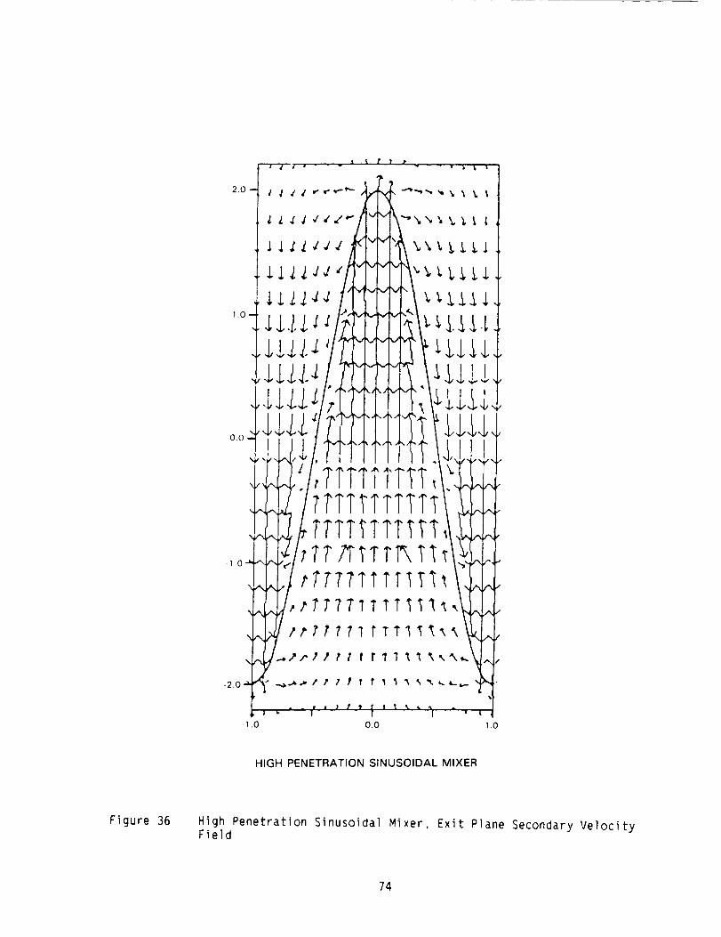
V

-I .0 0.0 1.0

HIGH PENETRATION SINUSOIDAL MIXER

Figure 36 High Penetration Sinusoidal Mixer, Exit Plane Secondary VelocityField

74

Measuredboundary layer parameters at this 1o::ation are given in Table D.4 and

are observed to be several times smaller than those for the low penetration

model which had a similar turbulent trip. This boundary layer reduction is

attributed to local flow acceleration in the thick (0.7) leading edge region

of the model.

Axial Velocity Field - The advanced high penetration model displayed a larger

region of inviscid flow within the interior c,f the lobes than either of the

sinusoidal mixers. This behavior is evident from Figure 37 which shows that the

(u+U_)/(].49 U_) = 0.99 contour extends upw_.rd to a value of y=0.81 at z=O

and downward to y= -0.75 at z=]. (In this corJ1parison,1.49 U_ is used for

normalization of the axial velocity componeni_ since this represents the local

freestream velocity in the vicinity of the m xer trailing edge. Flow

acceleration from U_to 1.49 U_was caused 01 the convergence of the tunnel

walls). Based on lobe peak coordinates of y=l.16 and -1.22 at z=O and l,

respectively, the above 0.99 contour location,s correspond to 70% of peak at

z=O and 60% of peak at z=l. Corresponding 0.39 contours for the low and high

penetration models extended only to zero and 50%, respectively.

The proportionately greater inviscid flow region for the advanced mixer

resulted in significantly greater effective penetrations. This greater

effective penetration is evident from the table below where boundary layer

transverses at the lobe exit plane are used to calculate displacement

thickness (see Table D.4) along lobe centerIines (z=O and l). Subtracting this

value from the lobe amplitude gives the effE_ctive lobe amplitude which can be

expressed as a percentage of physical amplilude. This percentage is termed

effective penetration.

75

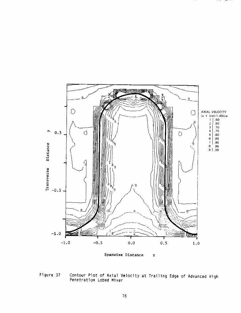
0,5

-i.0

©

9\

b

©

-0.5 1.0

AXIAL VELOCITY

(u + Uo=itl.49Uoo

1 .60

2 .65

3 .70

4 .75

5 .80

.85.90

8 .95

9 .99

Spanwise Distance z

Figure 37 Contour Plot of Axial Velocity at Trailing Edge of Advanced HighPenetration Lobed Mixer

76

Model

Location

EffectivePenetration(h-6*)xlO0

h

Low Penetration High Penetration Advanced High

Sinusoidal Sinusoidal Penetration

z= O,l z = O,l z=O z=l

83% 88% 97% 95%

Total Pressure Field - Normalized total pressbre distributions given in Table

D.3.4 confirm the previously presented axial velocity results which showed

inviscid flow extended further into the lobe nteriors than in the case of the

sinusoidal mixers. Complicating factors in these model comparisons is that the

advanced mixer was three times longer than the sinusoidal mixers but was

subjected to an overall favorable pressure gradient. These two factors have

opposite effects on boundary layer growth. Belween the axial station where the

lobes began to form (Station 56.5) and the trailing edge (Station 66),

however, average velocity increased by only IC,%based on the tunnel area

distribution. This acceleration appears to be too small to account for the

significant differences noted above.

A feature not previously discussed is the bour,dary layer buildup on the

parallel sidewalls of the mixer. Tabulated in Table D.4 are boundary layer

characteristics obtained from horizontal totai pressure transverses at the

locations shown in Figure 38. Proceeding from bottom to top of the lobe,

transverses labeled "4 IN, "3 IN" and "2 IN" ,,ielded 6* values of O.Oll, 0.019

and 0.026 indicating a general thickening of ,;idewal] boundary layer thickness

with increasing y. Traverse "l IN" at the lobe peak yielded the highest value

of 0.04l. Similar results apply to the adjacent downward facing lobe.

77

6 OUT

1 OUT

i 2 IN m

III[

3IN

4IN _.!

2 OUT

3 OUT_Z

4 OUT

_OUT

5IN

6IN

ADVANCED HIGH PENETRATION

Figure 38 Advanced High Penetration Lobe Trailing Edge Boundary LayerTraverse Locations

78

This increase of boundary layer thickness with lobe height would be expected

based on pressure gradient arguments given earlier. Both sinusoidal mixers

displayed the same behavior, however in those (ases, sidewall convergence,

resulting in reduced lobe width with increasin_i!y, fostered merging of

opposite surface boundary layers on lobe centerline (z=O). This then

contributed to peak region blockage and reduced effective penetration. An

advantage of the parallel-sided lobe, therefor(J, appears to be the constant

lobe width which does not contribute to boundary layer merging on lobe

centerline. Stated in another manner, low momentum boundary layer fluid,

driven to the peak region by inviscidly imposed pressure gradients, can

distribute itself over the greater surface are._ of the rounded, parallel-sided

lobe peak (as opposed to the more pointed sinu_:oidaI peak) thereby reducing

peak region blockage on lobe centerline (z=O).

In summary, axial velocity and total pressure ,Jata indicate substantially

reduced viscous retardation effects for the advanced high penetration model.

This will be shown in the following section to have a Favorable effect on the

transverse velocity component Field.

Transverse Velocity Field - Transverse velocitll components for the advanced

mixer displayed the same general pattern as the sinusoidal models, as shown in

the right portion of Figure 39, but were unsymmetrical due to the

unsymmetrical lobe geometry. A significant difference between this model and

the previously discussed sinusoidal models is that the transverse component

magnitudes achieved near ideal values as discussed below.

79

1.6

1.2

.8

.4

>-

z-OI-

OQ.W .0con'-w

03Z

n,"

-,4

-.3

-.I .2

(A)SPANWISE

COMPONENT

(B)

TRANSVERSE

COMPONENT

"-" -T -To_ -_-'T3

3 3 '--_ •0 0

0_ • 111 1 0 "_ •0

•--D,,, _,_-- • • 10i O

0 2 7 J7 0 0

• "--- "-'--I_ lo_

--O _ _ | _ ,.11,-- _ 10_0 1 6 J12 2 >"

• _ _,1_, I ,.I0.-.

0 2 6 i12

-o _ .-mD. _ _ • _ 10'0 1 7 12 3 0 n'-

w

• _ 10'-71,7- "3- o_0 1

-o .-m.- .-_I_ _ • _ 1o0 1 5 11 3 0

0 1

2 1

2 3

I

3 lll 3 0I

_ ..,4,-- _ _ 6

3 _11 3 1

w

3

\

2 5 7 9 10 21

I ! I.6 .8 1.0

I !0 .2 .4

L 10 15_ 18 I_ 2 _ 2 {

L 10 _ 7__20 _ 18 _ 17{

. 0{ _ I,J, _i, _iI

- ,f ,,{ I, i\

-' i ,i ,i',-l,..-=I I I I I

.2 .4 .6 .8 1.0

SPANWISE POSITION

Figure 39 Advanced High Penetration Mixer Transverse and Spanwise VelocityField

80

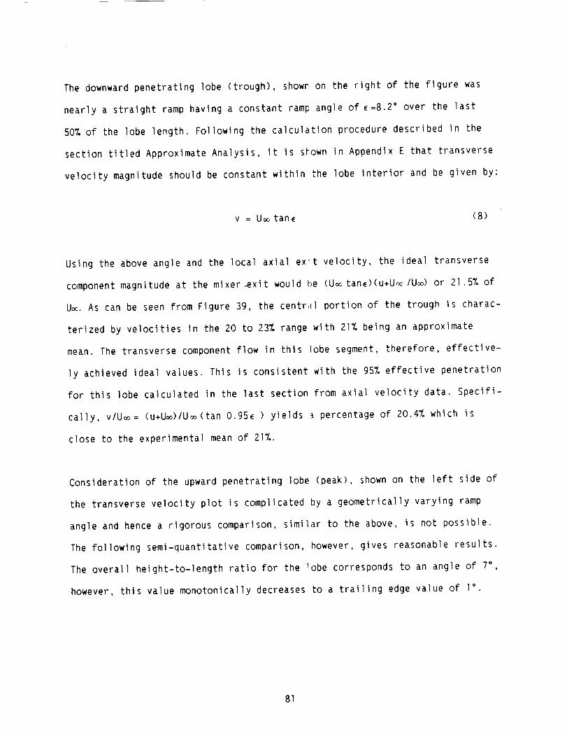
The downward penetrating lobe (trough), shown on the right of the figure was

nearly a straight ramp having a constant ramp angle of _=8.2 ° over the last

50% of the lobe length. Following the calculation procedure described in the

section titled Approximate Analysis, it is shown in Appendix E that transverse

velocity magnitude should be constant within the lobe interior and be given by:

v : U_tanE (8)

Using the above angle and the local axial exit velocity, the ideal transverse

component magnitude at the mixer mxit would be (U_ tanE)(u+U_ /Um) or 21.5% of

Um. As can be seen from Figure 39, the centr,_,1 portion of the trough is charac-

terized by velocities in the 20 to 23% range with 21% being an approximate

mean. The transverse component flow in this lobe segment, therefore, effective-

ly achieved ideal values. This is consistent with the 95% effective penetration

for this lobe calculated in the last section from axial velocity data. Specifi-

cally, vlU_= (u+Um)IUm(tan 0.95E ) yields _ percentage of 20.4% which is

close to the experimental mean of 21%.

Consideration of the upward penetrating lobe (peak), shown on the left side of

the transverse velocity plot is complicated by a geometrically varying ramp

angle and hence a rigorous comparison, similar to the above, is not possible.

The following semi-quantitative comparison, however, gives reasonable results.

The overall height-to-length ratio for the lobe corresponds to an angle of 7°,

however, this value monotonically decreases to a trailing edge value of 1°

81

Since a distance is required for the overall flow field to readjust to a

change in lobe slope, a intermediate effective ramp angle would be expected.

The measuredtransverse componentmagnitude of I0%U corresponds to an

effective angle of about 3.5° , which is plausible since this is the meanangle

over the last 30%of the lobe length (or about 1.2 times the peak-to-trough

lobe height). The above suggests that contouring a lobe to yield a smal] slope

at the lobe trailing edge is undesirable. Furthermore, maintaining a near zero

slope for several channel heights would be expected to effectively eliminate

the transverse componentresponsible for exit plane circulation and mixing.

Turbofan engine mixer geometries such as that studied by Paterson have a

decreasing slope in the trailing edge of the primary stream lobe. This is done

to prevent heating due to direct impingementon the tailpipe wall and high

expected turning losses. It is clear from the current study in which two lobes

of similar overall height-to-length ratio but differing rampangle schedules

(straight verses tapered) were investigated in the sameflow environment, that

ramp angle tapering has a strong negative influence on transverse component

magnitude and hence shed circulation.

One additional observation is useful relative to the data and approximate

analysis. The data shownin Figure 39 confirms the analytical result that

transverse componentmagnitude for a parallel-sided lobe is invariant with

respect to transverse position, y, within the lobe interior. This will be

shownsubsequently to be the cause of the higher exit circulation obtained

with this lobe relative to the sinusoidal lobes.

82

In summary,data from the straight-ramped downwardpenetrating lobe

conclusively showedthat the advancedmixer produced nearly ideal transverse

componentmagnitudes.

Spanwise Velocity Field - Spanwise velocity c::)mponentsfor the advanced mixer

were substantially different from the low and high penetration sinusoidal

models as shown in the left hand portion of Figure 39. This difference can be

attributed to the close proximity of the exit plane measurement station to the

trailing edge of this n_de (7 = 0.05). The trailing edge geometry was a

semicircle with a diameter of 0.06, hence the measurement station was only one

trailing edge thickness downstream of the bl_nt base. As shown in the study by

Paterson and Weingold (References 16,17), the near wake of such a trailing

edge consists of a closed recirculation bubble having a length of about one

trailing edge thickness. In response to the termination of the bubble in the

axial direction the flow is directed inward (,n both sides toward the trailing

edge centerline thereby filling in the wake behind the edge. Quantitatively,

Reference 16 shows that at one trailing edge thickness downstream of the

trailing edge, and one thickness offset from centerline, the inwardly directed

velocity component is 9% of the axial veloci;;y. This relative location

corresponds closely to the Figure 39 traverse at z=0.57 where values ranging

from 7 to ll% of U_ are observed on right side of the vertical portion of the

lobe. Values obtained along transverse lines at z=O.17, 0.37 and 0.77 are also

consistent with Reference 16 results. From t_is it is concluded that the

spanwise component field between y=-O.8 and ).8 is dominated by this near wake

effect. If taken further downstream at the _::0.36 Tocation used for the

previous models, ie. at seven trailing edge thickness downstream, Reference 16

shows these spanwise components would have decayed to levels on the order of

one percent.

83

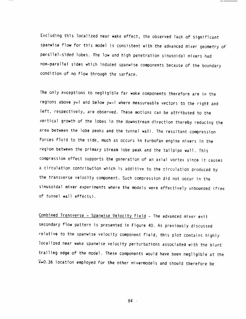
Excluding this localized near wake effect, the observed lack of significant

spanwise flow for this model is consistent with the advancedmixer geometry of

parallel-sided lobes. The low and high penetration sinusoidal mixers had

non-parallel sides which induced spanwise componentsbecauseof the boundary

condition of no flow through the surface.

The only exceptions to negligible far wake componentstherefore are in the

regions above y=1 and below y=-l where measureablevectors to the right and

left, respectively, are observed. Thesemotions can be attributed to the

vertical growth of the lobes in the downstreamdirection thereby reducing the

area between the lobe peaks and the tunnel wall. The resultant compression

forces fluid to the side, muchas occurs in turbofan engine mixers in the

region between the primary stream lobe peak and the tailpipe wall. This

compression effect supports the generation of an axial vortex since it causes

a circulation contribution which is additive to the circulation produced by

the transverse velocity component. Such compression did not occur in the

sinusoidal mixer experiments where the models were effectively unbounded(free

of tunnel wall effects).

Combined Transverse - Spanwise Velocity Field - The advanced mixer exit

secondary flow pattern is presented in Figure 40. As previously discussed

relative to the spanwise velocity component field, this plot contains highly

localized near wake spanwise velocity perturbations associated with the blunt

trailing edge of the model. These components would have been negligible at the

_=0.36 location employed for the other mixermodels and should therefore be

84

Figure 40 Advanced High Penetration Mixer Exit Plane Secondary VelocityField

85

disregarded when making comparisons. Figure 40 shows the same general

counter-rotating axial vortex pattern obtained with the sinusoidal models. The

resultant vortex circulation is presented in the section,"Circulation

Calculations".

B. Mixer Flow Analysis

In Section III, two inviscid linearized potential flow analyses (PLANMIX and

FLOMIX) were used to analyze the flow over the three lobed mixer contours for

which experimental measurements were presented in Section IV. The results of

these analyses, presented in Figures 6, II, and 12 show that the lobes induce

a spanwise or cross stream pressure gradient that force the flow off the crest

and into the trough. The experimental results presented in Section IV

furthermore showed that the sinusoidally shaped lobes did not achieve their

ideal levels of penetration, based on their lobe height to length ratio,

primarily due to a buildup of boundary layer flow in the trough. It was,

moreover, observed that the boundary layer distribution at the trailing edge

of the advanced high penetration lobe was more evenly distributed over its

surface area. An analytical solution of the lobe boundary layer development

was therefore made to see if these characteristics could be attributed to the

inviscid pressure gradient alone.

86

A calculation of the boundary layer development on the surface of the analyzed

mixer lobes was madeusing a three-dimension_l turbulent differential method

of Vatsa (Ref. 18, 19). This method is based on the two-dimensional concepts

of Blottner (Ref. 20) but was extended by developing a more suitable

transformation based on the Levy-Lees variables. The method has been used to

obtain solutions to a numberof complex turbomachinery problems. This

procedure has been also modified to treat arbitrary three-dimensional surfaces

using a nonorthogonal surface oriented coorcinate system (Ref. 21). The

inviscid surface flow field obtained from tr,e PLANIXor FLOMIXcodes was

adapted to this nonorthogonal frame of refeTence to provide edge conditions

for the boundary layer analysis.

The solution procedure is a forward marchinq algorithm, propagating

disturbances according to characteristic zc,ne of influence conditions. The

solution was initialized to march from the :nlet to lobe exit Dlane and march

off the lobe crest symmetryline to the lob_ trough. The calculation was

tripped to turbulent close to the inlet or eading edge and an equilibrium

turbulent profile was generated substantial y upstream of the lobe break

7ocation. The boundary layer calculations w_re made on a 100 by 100 surface

grid with 100 points normal to the surface.

The boundary layer results for the low and _igh penetration sinusoidal lobed

mixers are shown in Figures 41-43. Figure 41 shows a contour plot comparison

of the cross flow angle at the edge of the boundary layer (inviscid - from the

linear analyses) and the cross flow angle along the surface (viscid - from 3D

87

1.0

0.0

1.0

0.0

Inviscid Crossflow Contours Viscous Crossflow Contours

Trough

(:leg.

0.WOO

I. 0002.9003.0O84.000

5.000

Crest

]Trough

deg.

1 I 0.0090

2 [ 5.0803 10. O0

Crestr u J i I

(a) Low Penetration Sinusoidal Mixer Lobe

'.0

Trough

deg.

0. 00895.00010.8015.0020.88

Crest

/

\

I

i

Trough

deg.1 9.0000

2 5.0083 10.004 15.085 20.00G 25.007 30.00

Crest

I I| | , i

I0. 41.0

(b) High Penetration Sinusoidal Mixer Lobe

I I

I0.

Figure 41 Calculated Surface Inviscid and Viscous Crossflow Angle Contoursfor Sinusoidal Lobed Mixers

88

i.O(Trough'.

0.0(Crest)

High Penetration Sinu,,oidalLow Penet.ration Sinu',,oidal

v

l.-.-m-_

.b ll_

l I l0.7 0.8 0.9

Axial Distance x,Lm

l.O

(a) Inviscid Str(amlines

l.O

(Trough)

O.O

(Crest)

High Penetration Sinusoid_=l

Low Penetration Sinusoidal

i I l0.7 0.8 0.9 l.O

Axial Distance )/Lm

Figure 42

(b) Viscous Streamlines

Calculated Streamline Deflections dueEffects for Sinusoidal Lobed Mixers

to Inviscid and Viscous

89

boundary layer analysis). The plots have been plotted on on enlarged spanwise

scale. Onecan clearly see that viscous effects have significantly increased

the flow skewing on the high penetration mixer, but that the maximumskewing

effect still occurs at the trailing edge, midwaybetween the crest and trough.

The increase in skewing on the high penetration surface is about 50%over the

inviscid level. This trend is seen more clearly in the calculated streamline

patterns shownon Figure 42 (a) and (b). The lobe aspect ratio has beenmain-

tained here, so only the last third of the lobe surface has been displayed.

The effect of the viscous boundary layer on slow skewing is clearly notice-

able. The streamline deflection increase on the low penetration surface shown

in Figure 42 (a) is very slight, while the increased skewing angle fOr the

high penetration mixer, shownin Figure 42 (b) is so severe that one can

visualize the flow being swept off the crest and into the trough.

Finally, Figure 43 shows the trailing edge distribution of 699, the boundary

layer thickness, relative to that on an equivalent length flat plate. The

results show the same trends demonstrated experimentally in Section IV, i.e.

that the boundary layer is driven from the crest and that the trough boundary

layer is significantly increased. Furthermore, the boundary layer buildup

effect on the high penetration lobe is larger than that for the low

penetration lobe.

90

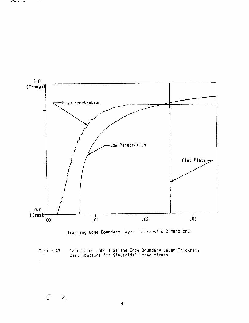
, v w_

l.O

(Trough) _

0.0

(.00

gh Penetration

tion

J

I I I

.01 .02 .03

I Flat Pla_

I

Trailing Edge Boundary Layer Thickness 6 Dimensional

Figure 43 Calculated Lobe Trailing Ed_iieBoundary Layer ThicknessDistributions for Sinusoida Lobed Mixers

91

C. Mixer Flow Field Model

1. Circulation Calculations

The most important single parameter describing the velocity field shed from

the mixer lobe trailing edge is the vortex circulation,Fproduced in each ]obe

segment and found by performing a contour integration in a p]ane norma] to the

axial direction. This circulation is related to downstream mixing rate as

discussed in the next section. In this section, vortex circulation is

calculated for the three mixer configurations by integrating experimentally

determined secondary ve]ocity fie]ds about an appropriate contour. Comparisons

are made with estimates derived from the approximate inviscid analysis.

Comparisons with FLOMIX results are given in the section titled Flow Analysis.

Referring to the integration path sketched below, exit plane circulation is

given by:

I' :I_-_.d-_ = Ivdy +I wdz +Ivdy + I wdz

s 1 2 3 4

=Fv +Fw

(9a)

(9b)

where the numbers refer to the integration paths shown in the sketch.

The quantities Fv andrw are the circulation contributions from the two

vertical and horizontal legs of the circuit, respectively. The circulation, r,

represents the strength of the vortex layer (or sheet) which is ]ocated along

the trailing edge surface and is shed into the wake. This circulation should

92

VORTEX LAYE RCROSS-HATCHED

, ' I I I%, / I ,SINUSOIDAL LOBE ADVANCED LOBE

be independent of the path choosen for integ'ation if the path encompasses the

entire sheet. The above path satisfies this equirement and has been chosen

for ease of integration.

Results of the circulation calculation are given in the table below. Row 1 of

the table gives absolute values of the circulation, based on experimental

data, for all three models in terms of U_ (tqe upstream freestream velocity)

and L, the lobe width on mixer centerline. The quantity L appears here, not

because it is a circulation parameter, but _ecause it has been used to

non-dimensionalize all distances in this re,oFt. The value of L for all three

models was 2.54 cm. As can be seen, the higf, penetration sinusoidal mixer had

the highest circulation, being 12.2 times larger than the low penetration

model. The advanced high penetration mixer _as intermediate between these two.

being 4.4 times larger than the circulation For the low penetration model. The

above has considered absolute levels of circulation per lobe segment for

models having significantly different geomelries. The next paragraph considers

the dependence of circulation on the import_:,ntgeometrical parameters.

93

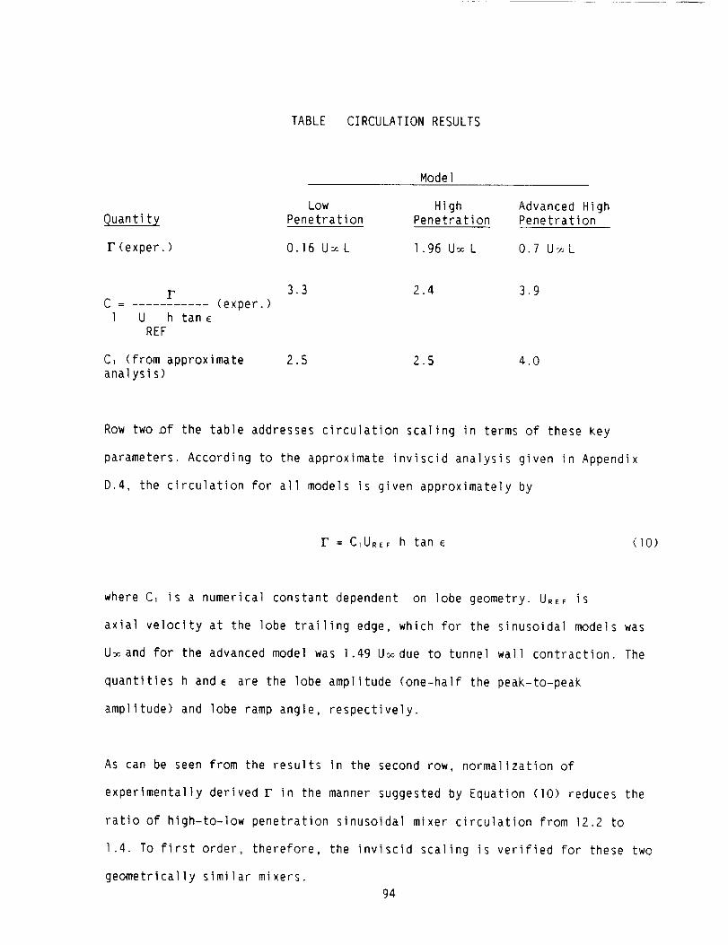
TABLE CIRCULATION RESULTS

Quantity

r (exper.)

rc = (exper.)1 u h tan E

REF

Model

Low High Advanced HighPenetration Penetration Penetration

0.16 U_L 1.96 U_L 0.7 U-_L

3.3 2.4 3.9

C, (from approximate 2.5 2.5 4.0

analysis)

Row two _f the table addresses circulation scaling in terms of these key

parameters. According to the approximate inviscid analysis given in Appendix

D.4, the circulation for all models is given approximately by

F = C_URE_ h tan E (10)

where C, is a numerical constant dependent on lobe geometry. URER iS

axial velocity at the lobe trailing edge, which for the sinusoidal models was

U_and for the advanced model was 1.49 U_due to tunnel wall contraction. The

quantities h and _ are the lobe amplitude (one-half the peak-to-peak

amplitude) and lobe ramp angle, respectively.

As can be seen from the results in the second row, normalization of

experimentally derived F in the manner suggested by EQuation (10) reduces the

ratio of high-to-low penetration sinusoidal mixer circulation from 12.2 to

1.4. To first order, therefore, the inviscid scaling is verified for these two

geometrically similar mixers.

94

Some complications ensue in obtaining C_ for ihe advanced mixer because the

ramp angle was different for adjacent lobes. As discussed in the section

titled "Transverse Velocity Field", ramp angles for the two lobes were derived

to be 8.2 deg. and 3.5 deg. Use of the average of these angles (5.85 deg>

leads to the constant of 3.9 shown. The higher value of the constant relative

to the sinusoidal mixers is due to the more effective parallel-wa11 geometry

of the advanced mixer. This circulation enhanc;ement is confirmed in row three

where the theoretical constants C,, derived in Appendix D.4, are given for

sinusoidal and parallel wall geometries. As c,Ln be seen, the parallel walled

lobe circulation is predicted to be higher th,_n the sinusoidal lobe

circulation and is in close agreement with exi)eriment.

Since the approximate analysis is a one-dimen_;ional calculation it can be

expected to be most accurate in the limit of large sinusoidal amplitude (high

aspect ratio lobes have a flow which is close to one-dimensional) and this is

observed to be the case based on the close ageement of experimental and

theoretical C_ constants for the high penetration sinusoid. As shown in

Appendix D.4, the sinusoidal mixer calculatio_ neglects contributions from the

horizontal legs of the circuit shown above. Based on data, this contribution

to total circulation was negligible for the lirge aspect ratio sinusoidal

mixer (only 2%) but appreciable for the low penetration sinusoid (24%). The

more two dimensional flow character of the Io_ penetration sinusoid,

therefore, is the reason for the discrepancy between measurement and analysis

shown in column I. The parallel-sided lobe calculation is the most accurate

95

since there is no horizontal leg contribution and the flow is inherently

one-dimensional by virtue of the parallel walls. In summary,for

parallel-sided lobes or sinusoidal lobes having the high aspect ratio

necessary to produce large circulations, the approximate calculation gives a

good estimate of the circulation shed at the mixer trailing edge.

One conclusion resulting from the above is that the approximate circulation

scaling given by Equation (lO) is supported by the data. A second conclusion

is that the advancedmixer, having parallel sidewalls, is inherently superior

in terms of circulation, to sinusoidal lobes (that is, for similar rampangle

and lobe amplitude, the ratio of parallel walled to sinusoidal lobe

circulations would be 4.0/2.5 or 60% greater). In fact the approximate

analysis in Appendix D.4 shows that the more pointed the lobe, the lower the

value of C,, ie. parallel-walled lobes, sinusoidal lobes and triangular

lobes have constants of 4, 2.5 and 2, respectively. The relatively high C,

value of 3.3 obtained experimentally for the low penetration sinusoidal is not

practica]ly important, because to achieve the C, benefit for a fixed lobe

length Lm, lobe amplitude, h, must be reduced dramatically and the scaling

showscirculation is proportional to the square of this amplitude, ie.

£ _h tan E _hZ/L_ (ll)

where L_ is lobe axial Length. A low penetration sinusoidal mixer, such as

considered here, therefore, will produce a high C, constant but poor

circulation per lobe segment.

96

2. Circulation and Mixin 9

This section discusses the effect of lobe e<it circulation and other lobe

parameters on downstream mixing. From the s!:andpoint of mixing it is believed

that maximizing circulation per lobe segment is advantageous. This is the

basic conclusion of Paterson's previous for_:ed mixer nozzle study. As shown by

Equation (I0), this can be achieved, in part, by using the largest ramp angle,

E, that does not cause separation within the lobe. This is a strong effect

since circulation is proportional to the square of lobe amplitude. Tapering

ramp angles at the trailing edge of a lobe is clearly undersirable.

Circulation can also be increased by accelerating flow within the lobes to

produce a higher exit plane UREF. Such acceleration is also desirable to

thin lobe boundary layers and reduce lobe peak blockage. Circulation can also

be enhanced by selecting geometries having high C, constants. For planar

configurations, purely rectangular lobes have the highest theoretical value

but rectangular lobes with rounded peaks ar, d troughs may be superior because

corner secondary vortices and flow separation off the ramp in the outer flow

can be avoided. Such vortices were found b_ Paterson (Reference 4) in a survey

downstream of rectangular lobes.

Lobe segment circulation is not the only p,,rameter affecting downstream

mixing. Lobe width is another free and important parameter. It is clear that

extremely narrow lobes will behave poorly because sidewall boundary layers

will merge on lobe centerline producing vi._.cous losses and reduced circulation

due to increased peak region blockage. Ver_ wide lobes, however, are

undesirable since the average vorticity pe_ lobe segment is reduced. This can

be seen, for example, in the following exp_ession for a rectangular lobe. For

such a lobe, average vorticity per lobe, _ , is given by:

97

2U tanF REF

co ..... + (12)2hL L

Stated in a different manner, vortex sheets (concentrated along the lobe

sidewall trailing edges) will roll-up to produce a vortex having some

characteristic lateral scale. If this scale is small relative to lobe width,

then regions of irrotational flow will exist between adjacent counter rotating

vortices. These irrotational flow regions will mix out slower than those

regions containing vortices and mixing will be degraded. Improved

understanding of the effect of L on mixing can only come from mixing

calculations. This is also true of the remaining mixing parameter which is the

lobe penetration (ratio of lobe height to mixing duct height).

In summary, this study produced insight into the lobe circulation development

process. It now remains to extend the preliminary calculation shown in

Appendix A, where the FLOMIX lobe calculation was coupled with a downstream

mixing calculation and to perform a comprehensive parameter variation study on

the effects of lobe penetration and lobe width for various lobe geometries and

selected values of ramp angle and URE,. This should be complemented by

experiments in which mixing is measured (eg. using a cold and warm stream

configuration to permit temperature to be used to define mixing) at several

downstream locations for selected designs. For planar configurations, the

prime emphasis should be on the parallel-sided geometry shown here to maximize

circulation. For other geometries, such as axisymmetric, the approximate

inviscid analysis can be used to identify preferred geometries.

98

It is also clear that further experimental anc analytical research is needed

in the area of vortex dynamics. For similar values of lobe segment

circulation, different lobe width-to-lobe hei_i_ntratios would be expected to

affect vortex roll-up. Thus while designing l(:bes to maximize circulation is

important, this is not sufficient to maximize downstreammixing ratio.

Vl. SUMMARYOF R[SULTS

l o Experiments conducted with three planar mLxer lobe models confirmed the

findings of a previous research program tilat lobed mixers produce a

periodic array of adjacent, contrarotating streamwise vortices downstream

of the lobe exit plane. The transverse scale of the vortices is comparable

to the lobe-to-peak amplitude and the spa_wise scale of each vortex is

one-half of the periodic lobe wave length.

. Planar and axisymmetric linear inviscid analyses were developed to predict

the secondary velocity fields and vortex circulations at the exit plane of

periodic lobed mixers. A coupled three-dimensional boundary layer analysis

was applied to predict exit plane boundarv layer characteristics. These

analyses were then used to predict flow cevelopment for the three mixer

configurations studied experimentally. Acditionally, an approximate

inviscid analysis was developed to identify scaling parameters for lobe

circulation and to assess waveform geomelry effects on exit plane

circulation.

99

. Transverse velocity component measurements at the exit plane of the three

models tested showed significant cross-stream flows in the direction of

the lobe peak on the order of IO - 30% of the lobe exit axial velocity.

Magnitudes were largest for high penetration sinusoidal model which also

has the largest lobe amplitude. Transverse velocity magnitudes diminished

in the interior lobe peak region of the sinusoidal models whereas the

advanced mixer displayed near ideal velocity levels well into the lobe

peak.

, Axial velocity and total pressure measurements at the exit plane of the

two sinusoidal waveform mixers indicated significant viscous retardation

effects occurred w%thin the peak interior region of the lobes. Similar

measurements for the advanced mixer showed much thinner lobe boundary

layers with inviscid flow extending well into the rounded lobe peak region.

5. Spanwise velocity component magnitudes at the lobe exit plane were

substantially smaller than the transverse component for all three models.

, Surface flow visualization of the lobes showed skewing of the near surface

flow toward the lobe peak and trough regions. As expected, the degree of

skewing was greatest for the two high penetration models.

100

VII. CONCLUSIONS

I o The array of large scale, streamwise vortice_ shed from the trailing edge

of convoluted lobe mixers is a consequence of the combined transverse and

spanwise pressure field created by lobe penetration into the approaching

stream. Cross-stream pressure gradients in conjunction with a lobe

trailing edge Kutta condition create a press,Jre driven secondary flow

field having significant transverse velocity components. Cross-stream

pressure gradients also cause skewing of the lobe boundary layer toward

the lobe peak and trough regions, the origic of the streamwise vortex

array is basically inviscid in nature.

o Linear inviscid analyses developed in this _tudy, in conjunction with a

three-dimensional boundary layer analysis, e_re capable of predicting lobe

streamwise vortex array characteristics. PrE_dicted lobe exit plane

streamwise vortex circulations and boundary layer characteristics were

found to be in favorable agreement with current experimental results.

Since the lobe flow was found to be invisci(i, a boundary layer analysis is

only needed if details inside the viscous r(,gion are needed.

. An approximate inviscid analysis identified the primary parameters

affecting exit plane circulation for straight ramped lobes as the ratio of

lobe amplitude squared-to-lobe length, exit plane axial velocity and a

lobe shape factor which varies with lobe sp_nwise waveform. Circulation is

found to be equal to the product of these f_ctors, therefore exhibiting a

strong dependence on lobe amplitude. Experinental data obtained in the

study confirmed the lobe amplitude and axial velocity scaling.

101

o The lobe shape factor is highest for parallel-sided lobe configurations

(similar to the advance high penetration mixer tested in the study). Such

configurations are inherently superior to non-parallel walled

configurations such as sinusoidal or triangular. Experimental data

obtained in the study confirmed the predictions relative to parallel-sided

and sinusoidal configurations.

. The advanced mixer model tested in the program nearly achieved the ideal

exit plane circulation predicted by an inviscid analysis. In addition to

an inherently lower circulation geometry, the two sinusoidal mixer models

were adversely affected by boundary layer buildup in the interior peak

region of the lobes. This reduced the effective lobe amplitude and

consequently the circulation shed into the wake.

. The final conclusion of this study is that future work should be directed

toward integration of the linear inviscid analysis into an overall mixer

mixing analysis permitting mixing calculations to be performed for a

series of lobe geometrical parameters. A complementary experimental study

of downstream mixing should also be performed thereby providing a verified

overall design analysis system for use in turbofan engine, ejector and

other convoluted lobe mixing applications.

I02

l .

°

°

,

.

,

°

REFERENCES

Presz, W. M., Jr., Gousy, R., and Morin B.." Forced Mixer Lobes in EjectorDesigns," AIAA 86-1614, AIAA/ASME/SAE/ASEE 22nd Joint PropulsionConference, Hustsville, AL, 1986.

Werle, M. O., Paterson, R. W., and Presz W. M., Jr., "Flow Structure in aPeriodic Axial Vortex Array," AIAA 87-0610.. AIAA 25th Aerospace SciencesMeeting, Reno, NV, 1987.

Nerle, M. J., Paterson, R. W., and Presz, ;_. M., Jr.," Trailing-EdgeSeparation/Stall Alleviation," AIAA Journal, Vol. 25, No. 4, 1987, p. 624.

Paterson, R.W., "Turbofan Forced Mixer-Nozzle Internal Flowfield,Part I - A Benchmark Experimental Study," '_ASA CR 3492, April, 1982. AlsoASME Journal of Engineering for Gas Turbinas and Power, Vol. 106, July1984, pp. 692-698.

Povinelli, L., Anderson, B., and Gerstenmaier, W., "Computation of theThree-Dimensional Flow in Turbofan Mixers _nd Comparison Nith ExperimentalData," AIAA Paper 80-0227, Jan. 1980.

Anderson, B., Povinelli, L., and Gerstenmaier, N., "Influence of PressureDriven Secondary Flows on the Behavior of Turbofan Forced Mixers," AIAAPaper 80-I198, AIAA/ASME/SAE 16th Joint Propulsion Conference, July, 1980.

Povinelli, L.A.., and Anderson, B.H., "Investigation of Mixing in aTurbofan Exhaust Duct, Part II: Computer Code Application andVerification," AIAA J., Vol. 22, No. 4, 1984, p. 518

8. Amiet, R.K., "User's Manual a Laterally Planar Inviscid Mixer Analysis,"

Pratt & Whitney Report PNA-5904-18, 1983.

. Barber, T.J., "Turbofan Forced Mixer Lobe Flow Modeling, Part II: -Three-Dimensional Inviscid Mixer Analysis (FLOMIX)," to be published as aNASA CR ×XXX, 1986.

I0. Barber, T.J., Muller, G.L., Ramsay, S.M., and Murman, E.M., "Three-Dimensional Inviscid Flow in MIxers, Part [: Mixer Analysis Using a

Cartesian Grid," AIAA J of Propulsion &Pcwer, Vol. 2, No. 3, 1986, P. 275.

II. Barber,AT.J., Muller, G.L. Ramsay, S.M., end Murman, E.M.,"Three-Dimensional Inviscid Flow in MIxer_, Part 11: Analysis of Turbofan

Forced Mixers," AIAA J Propulsion & Power, Vol. 2, No. 4, 1986, p. 339.

12. Larkin, M.J., and Blatt, J.R., "Energy Efiicient Engine Exhaust Mixer

Model Technology Report Addendum-Phase II] Test Report," NASA CR 17499,1984.

13. Maskew, B. "Prediction of Subsonic Aerodyr_amic Characteristics: A Case for

Low-Order Panel Methods," AIAA J Aircraft. Vol. 19, No. 2, 1982, p.157

103

14. Clark, D.R., Maskew,B., & Dvorak, F.A., "The Application of a SecondGeneration Low-Order Panel Method--ProgramVSAERO--to PowerplantInstallation Studies," AIAA Paper 84-0122, AIAA 22nd Aerospace SciencesMeeting, Reno, NV, 1984.

15. Coles, D. E., "The Turbulent Boundary Layer in a Compressible Fluid,"Report R-4-3-PR, RandCorporation, Santa Monica, CA, September1962.

16. Paterson, R. W., and Weingold, H. D.," SupercriticaI Airfoil TechnologyProgram," Pratt & Whitney Aircraft, FR-15859,October ]982.

17. Paterson, R. W., and Weingold, H. D.," Experimental Investigation of aSinu]ated CompressorAirfoil Trailing Edge Flowfield," AIAA Journal, VoI.21, No. 5, 1985, p. 768.

18. Vatsa, V. N., "A Three-Dimensional Boundary Layer Analysis Including HeatTransfer and Blade Rotation Effects," Third Symposiumon Numerical andPhysical Aspects of Aerodynamic Flows, Long Beach, CA, 1985.

19. Vatsa, V. N., "A Three Dimensional Boundary Layer Analysis forTurbomachinery Applications," UTRCRepOFt84-44, 1984.

20. Blottner, F. G., "Computational Techniques for BoundaryLayers AGARDLecture Series 73, presented at VKI, February 1985.

21. Anderson, O. L., "Assessmentof a 3-D Boundary Layer Analysis to PredictHeat Transfer and Flow Field in a Turbine Passage," UTRC ReportR85-956834, also NASA CR-174894, 1985.

A.I Briley, W.R., and McDonald, H., "Analysis and Computation of Viscous

Subsonic Primary and Secondary Flows", AIAA 4th Computational Fluid

Dynamics Conference, Williamsburg, VA, 1979.

A.2 Kreskovsky, J.P., Briley, W.R., and McDonald, H., "Development of a Methodfor Computing Three-Dimensional Subsonic Turbulent Flows in Turbofan Lobe

Mixers", Scientific Research Associates, Inc., R79-300006-F, 1979.

104

APPENDICES

A. Viscous Marching Analysis

B. Lobed Mixer Coordinates

I. Low Penetration Sinusoidal Lobed Mixer

2. High Penetration Sinusoidal Lobed Mixer

3. Advanced High Penetration Lobed Mixer

C. Code Input Files

I. PLANMIX: Low Penetration, High Penetration

2. FLOWMIX: Low Penetration, High Penetration, Advanced High Penetration

D. Experimental Data Base

I. Low Penetration: U+u,v,w and Pt data

2. High Penetration: U+u, v, w and Pt data

3. Advanced High: U+u,v, w and Pt and BoLndary Layer Data

4. Boundary Layers

105

APPENDIXA

VISCOUSMARCHINGANALYSIS

An analytical study was performed to demonstrate the influence of pressure

driven secondary flows on the behavior and performance of turbofan forced

mixer nozzles. The viscous marching analysis used in this study was the PEPSIM

approach developed by Briley, McDonaldand Kerskovsky (Ref. AI, A2). The

procedure is based on the decomposition of the velocity field into primary and

secondary flow velocities. The governing equations are solved by a forward

marching method, where elliptic effects due to curvature and area changeare

accounted for a priori through the imposedpressure gradients determined from

a potential flow solution for the geometry in question. The inflow conditions

entering the mixing duct were varied to demonstrate their effect on the mixing

rate at the nozzle exit plane. In previous analytical studies, the secondary

flow effect was represented as a superimposed radial velocity basedon a

factor of the local mainstream velocity.

In the present study, the benchmark experimental study of the JT8D-209 forced

mixer was considered. Mixing predictions have been made using the PEPSIM

anlysis for the following inflow profiles:

I. the measured mixer lobe exit plane data,

2. an ideal inflow profile with no cross flow velocity field, and

3. an ideal inflow profile with a superimposed secondary flow field.

106

The ideal profile consists of a uniform primarl and bypass profile separated

by an assumedor estimated shear layer interfa_:e. In the latter case, a

series of calculations were madewhere the degree of secondary flow was

parametrically varied. The primary measureof neasuring the mixing

effectiveness of a specific input profile was the predicted total temperature

profile. Exit plane profile comparisons with t_e measuredtraverse data were

madeat three equally spacedazimuthal cuts. A partial display of the results

of this study is presented in Figure A.I. The ;op comparison indicates that by

starting the calculation with the actual mixer lobe exit plane profile, one

can obtain a reasonable level of agreementwith the measuredprofiles. In

contrast, the ideal profile input case showsvery little agreement. At the

bottom of the figure, one particular estimated secondary flow case is

presented. The magnitude of the superimposed p_imary and secondary radial

flows were estimated from the exit slope of the lobe crest and trough,

respectively. The predicted profiles show some disagreement in level, however,

they do follow the radial trends of the measured data. The analytical

predictions therefore demonstrate that the driving mechansism of the forced

mixer is the inflow secondary flow and that this effect can be modeled in an

empirical fashion.

107

1.00-

1

2.80_

0.80

0.40"

MIXER EXIT

O "_"

o 0-.\

0.20] c3:_._ _ _ _0.000.40 o./_o 2.i3o 1.00

O'

8 o

8'

2

00.4

°!°o

\O

0.6 0.8

NO77LE EXIT

O A

I /°/ o A

/ O ."I

( o t "

I o { ,.,

I o \ ,,,

I o _\ o ._\

NO "

): ,_ : o t41.0 026 0.8o_6 o18 1:o

(a) DATA INPUTSTART

11o

1.0

0.8

0.6

0.4

- \

0.2- _.

A

o0.4 0'.6

\ o

\ "o !\ °%

A

0'.8 1.0

1.0"

0.8"

0.8"

0.4"

0.2"

0.00.4

O

o_ \ o a0 1 ,h,

o\0 ,*,,,

o \ "

o _ o \ "/

0 1 0 \ ZZ

O 0 \

0 0 \

0 0 -"

0 0 _

o o I ,,

O, O I • _.

o'.6 0.8 £0 0.6o._ o18 o'.8 _;o

(b) IDEALSTART

\

\I

0.8 _:o

0.8I

0.6_ °\iz_ \_ = {3

--_ .4 \

\

0.4 o:8 0:8 _.o

Figure A.I

1,0'

0.8"

0,8"

0.4-

00.4

0.2

0

o°/ "o° °_ _:

/ 0 / A

/ ° /,,° / °

+ FLAP EFFECTo\

Ooi:/ ooo_oo _ _1 A _A''_,,,,.,. I

o'.6 8:8 1:o o I o:8 ,_ I 'o0.8 1.

0.4 06 0:8 11o

Effect of Starting Conditions on PEPSI-M Calculated Temperature

Ratio Profiles at Inlet and Exit Planes of JT8D-209 Mixing Duct.

(--,oO'=o;--_--_ O' =5; -,_e']08

TABLE B. l

LOW PENETRATION LOBED MIXER COORDINATES

1

2

3

4

5

6

7

8

9

i0

ii

12

13

14

15

16

17

18

19

2O

21

AXIAL COORDINATE

X(I)

0.00000

0.51547

0.92784

1.44330

1.95877

2.47423

2.98969

3.50516

4.02062

4.43299

4.94845

5.46392

5.97938

6.49485

7.01031

7. 52577

7.93814

8. 55670

8.96907

9.48454

10.00000

RA5 IAL COORDINATE

YCREST( I )

0.I0014E-04

0.I0014E-04

0.I0014E-04

0.19997E-04

0. 79989E-04

0. 31999E-03

0. 12100E-02

0. 37900E-02

0.99900E-02

0. 19290E-01

0. 38440E-01

0. 67200E-01

0. I0506E+00

0. 14986E+00

0 19891E+00

0 25000E+00

0 29148E+00

0 35398E+00

0 39570E+00

0 44785E+00

0 50000E+00

EQUATION OF LOBE CROSS-SE CTION

Y(I) = YCREST(I)* cos l--2c--Z(I)I

O{ ----Q = I-[

I09

TABLE B. 2

HIGH PENETRATION LOBED MIXER COORDINATES

1

2

3

4

5

6

7

8

9

i0

ii

12

13

14

15

16

17

18

19

20

21

AXIAL COORDINATE RADIAL COORDINATE

X( I ) YCREST (I )

0.00000 0.00000E+00

0.51547 0.00000E+00

0.92784 0.I0002E-03

1.44330 0.I0002E-03

1.95877 0.30005E-03

2.47423 0.13000E-02

2.98969 0.48000E-02

3.50516 0.15200E-01

3.91753 0.33400E-01

4.53608 0.89600E-01

4.94845 0.15380E+00

5.46392 0.26880E+00

5.97938 0.42020E+00

6.49485 0.59940E+00

7.01031 0.79560E+00

7.52577 0.10000E+01

8.04124 0.12075E+01

8.55670 0.14159E+01

9.07217 0.16245E+01

9.58763 0.18331E+01

10.00000 0.20000E+01

EQUATION OF LOBE CROSS-SECTION

Y(I) = YCREST(I) * CosI_Z(I) I

O_ ----Q -- 11"

110

TABLEB.3.1ADVANCED HIGH PENETRAT ILION

LOBED MIXER COORDINATES

RADIAL COORDINATES

I AXIAL COORDINATE YCREST(I)* YTROUGH(I)*

1 46.000 -0.138 0.575

2 47.000 -0.138 0.575

3 48.000 -0.138 0.571

4 49.000 -0.138 0.550

5 50.000 -0.138 0.509

6 51.000 -0.138 0.449

7 52.000 -0.138 0.376

8 53.000 -0.138 0.308

9 54.000 -0.138 0.230

I0 54.694 -0.138 0.179

Ii 55.000 -0.134 0.154

12 55.500 -0.116 0.112

13 55.600 -0.110 0.103

14 55.700 -0.104 -

15 55.800 -0.097 0.085

16 55.900 -0.089 -

17 56.000 -0.081 0.066

18 56.100 -0.071 -

19 56.200 -0.060 0.046

20 56.300 -0.049 -

21 56.400 -0.036 -0.033

22 56.500 0.036 -

23 56.600 0.049 -0.052

24 56.700 0.062 -

25 56.800 0.076 -0.070

26 56.900 0.090 -

27 57.000 0.105 -0.089

28 57.500 0.186 -0.137

29 58.000 0.268 -0.190

30 58.500 0.351 -0.244

31 59.000 0.434 -0.305

32 60.000 0.599 -0.429

33 61.000 0.766 -0.563

34 62.000 0.926 -0.703

35 63.000 1.055 -0.849

36 64.000 1.151 -0.992

37 64.500 1.180 -1o065

38 65.003 1.200 -1.137

39 65.600 1.210 -1.208

40 66.000 1.216 -1.281

* Y +/- 0.020

Ill

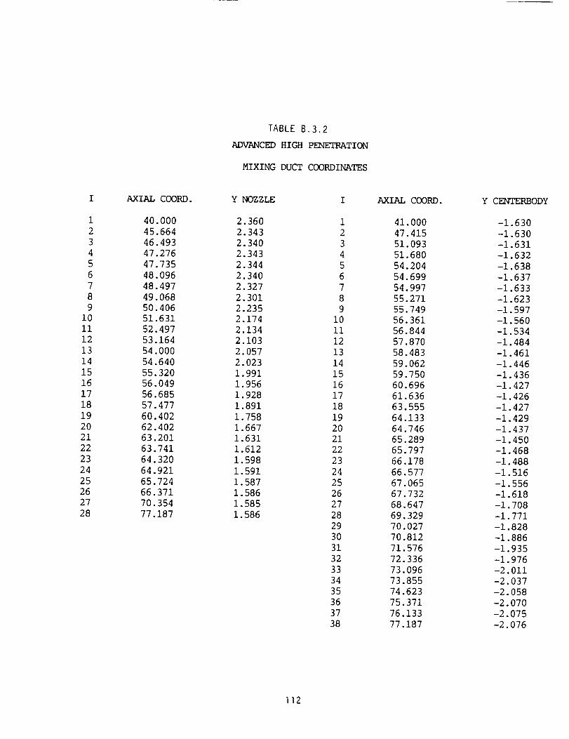
TABLE B.3.2

ADVANCED HIGH PENETRATION

MIXING DUCT COORDINATES

1

2

3

4

5

6

7

8

9

i0

ii

12

13

14

15

16

17

18

19

20

21

22

23

24

25

26

27

28

_IAL COO_. Y NOZZLE I

40.000 2.360 1

45.664 2.343 2

46.493 2.340 3

47.276 2.343 4

47.735 2.344 5

48.096 2.340 6

48.497 2.327 7

49.068 2.301 8

50.406 2.235 9

51.631 2.174 10

52.497 2.134 ii

53.164 2.103 12

54.000 2.057 13

54.640 2.023 14

55.320 1.991 15

56.049 1.956 16

56.685 1.928 17

57.477 1.891 18

60.402 1.758 19

62.402 1.667 20

63.201 1.631 21

63.741 1.612 22

64.320 1.598 23

64.921 1.591 24

65.724 1.587 25

66.371 1.586 26

70.354 1.585 27

77.187 1.586 28

29

30

31

32

33

34

35

36

37

38

AXIAL COORD.

41.000

47.415

51.093

51.680

54.204

54.699

54.997

55.271

55.749

56.361

56.844

57.870

58.483

59.062

59.750

60.696

61.636

63.555

64.133

64.746

65.289

65.797

66.178

66.577

67.065

67.732

68.647

69.329

70.027

70.812

71.576

72.336

73.096

73.855

74.623

75.371

76.133

77.187

Y CENTERBODY

-1.630

-1.630

-1.631

-1.632

-1.638

-1.637

-1.633

-1.623

-i. 597

-I. 560

-1.534

-1.484

-1.461

-1.446

-1.436

-1.427

-1.426

-1.427

-1.429

-1.437

-1.450

-1.468

-1.488

-1.516

-1.556

-1.618

-1.708

-1.771

-1.828

-1.886

-1.935

-1.976

-2.011

-2.037

-2.058

-2.070

-2.075

-2.076

112

TABLEC. 1

Low Penetration Mixer

MIXER TEST CASE

196 0.0

81 41 0

1.0 1.0

SVMESH

SXYO=O., SYZ0:0.,

DSXY=81*. 125,

DSYZ=41* .025

Sm_D

.215

0.5

3.14159

0.0

•0220977

Hi9h Penetration Mixer

MIXER TEST CASE

196 0,0

41 41 0

1.0 1.0

SVMESH

SXYO=O. ,SYZ0:0.,

DSXY=4 i* .25,

DSYZ=41*.025

SEND

.215

2.0

3.14159

0.0

.0883908

113

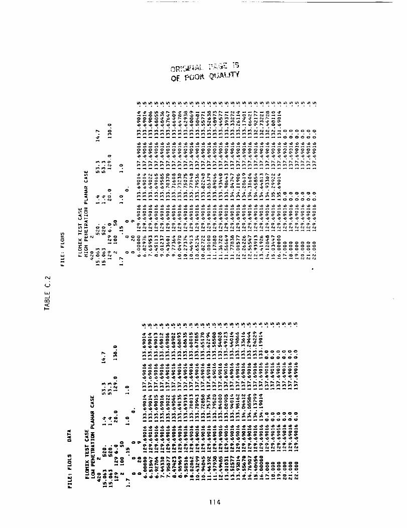
Of_ pOOR ._UAL_._f

(J7

gw.

_5

..--J

nr_

I---

o

r_

o

L_ _

_(

Q_,_ OZ

n_J 0 . ¢_

q[ i._C,J)--

I*-Q_ • • O t_**

m_

,.°°.o,°**°.°, ............... .°

• . , ..... , • • , , , , 0 . , , , . • • • •

_____oooooo

o_ ...............................

O

.JO

114

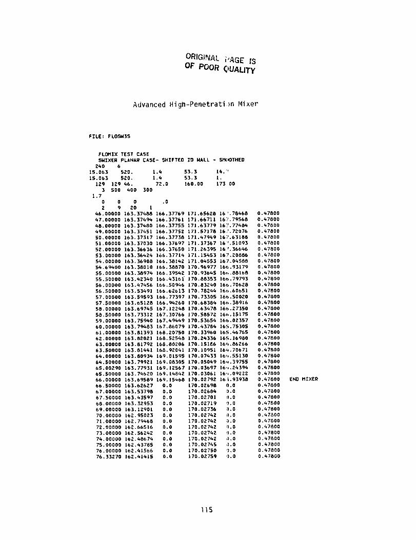
ORIGiF'JAL PAGE fS

OF POOR QUALITY

Advanced High-Penetrati,)n Mixer

FILE: FLOSMSS

FLOMIX TEST CASE

SNIXER PLANAR CASE- SHIFTED IO MALL - SMOOTHED

240

15.06315.063

129

31.7

0 0

Z 9

46.0000047.00000

48.00000

49.00000

50.0000051.00000

52.00000

53.0000054.00000

54.69400

55.00000

55.5000056.00000

56.50000

57.00000

57.5000058.00000

58.50000

59.0000060.00000

61.0000062.00000

63.00000

63.5000064.00000

64.50000

65.00290

65.5000066.00000

66.5000067.00000

67.50000

68.00000

69.0000070.00000

71.00000

72.0000073.00000

74.00000

75.0000076.00000

76.33270

6520. 1._ 53.3 14.':'

520. 1.4 53.3 1.

129 46. 72.0 160.00 17300

500 400 300

0

20 1

163.37488163.37494

163.37480

163.37_51163.37317

163.37030

163.36636

163.364Z_163.36908

163.38010

163.3897_163.42340

163.47456

163.53491

163.59593163.65128

163.697_5163.73312

163.759_0

163.79483

163.81393163.82021

163.81792

163.81441163.80934

163.79921

163.77931163.74620

163.69589

163.62627163.53798

163.43597

163.32953163.12901

162 95023

162 79468

162 66516162 56242

162 4867_162 43785

162.61566

162.41615

.0

166 37769

166 37761

166 37755

166 3775Z166 37738

166 37697

166 37650

166 37719166 38142

166. 38870166. 39562

166.43161"

166.50946

166.62613

166.77]97166. 94260

167. 12248167. 30766

167.49_69

167.86079

168. 20750168. 52548

166.80206

168.92041169.01595

169.08305169. 12567

169. 148_2

169. 154680.0

0.0

0.0

0.00.0

0.0

0.00.0

0.0

0.00.0

0.00.0

171.65628 16";'.78668 0.47800

171.66711 167.79568 0.47800

171.63779 16"7.77484 0.47800171.57178 167.72076 0.47800

171.47969 16"7.63188 0.47800

171.37367 167.51093 0.47800171.26395 167.36666 0.47800

171.15453 167.20886 0.67800

171.04553 167.04588 0.47800

170.96977 166.93179 0.47800170.93645 16_.88168 0._7800

170.88353 166.79793 0._7800

170.83240 166.70628 0.67800170.78266 166.60651 0.47800

170.73305 16_.50020 0.67800

170.68386 16_.38916 0.47800

170.63478 16_.27350 0.67800170.58572 166.15175 0.67800

170.53656 166.02357 0.67800

170.;3786 165.75305 0.47800170.31960 165.46765 0.47800

170.26336 165.16980 0.47800170.151_,6 16_.86266 0.47800

170.10951 16_.70671 0.47800

170.07433 16_.55130 0.47800

170.05069 16_.39755 0.47800170.03697 16':_.243c_ 0.47800

170.03061 16':_.09222 0.47800170.02792 165.93938 0.47800 END MIXER

170.02698 0.0 0.47800

170.02686 0.0 0.47800

170.02701 _).0 0.47800170.02719 i).O 0.47800

170.02736 _.0 0.47800

170.02762 _).0 0.47800170.02742 0.0 0.47600

170.02742 o.0 0.47800

170.0Z742 0.0 0.47800170.02742 _}.0 0.47800

170.02745 _.0 0.47800170.02750 0.0 0.67800

170.02759 _.0 0._7800

115

TABLE D.I.I

Low Penetration Lobed Mixer, (u+Um)/U_

Normalized Axial Velocity LV Data

Axial Location X = 0.36

Z

0 .i0

0.20

Y=0.72

0.992

0.996

Z Y=0.62 Z Y=0.52 Y=0.42

0.00 0.984 0.00 0.572 0.00 0.703

0.07 0.986 0.09 0.613 0.09 0.700

0.13 0.989 0.ii 0.613 0.ii 0.684

0.17 0.992 0.14 0.695 0.15 0.620

0.23 0.993 0.16 0.769 0.17 0.594

0.27 0.993 0.19 0.868 0.19 0.600

0.33 0.996 0.21 0.918 0.21 0.593

0.37 0.996 0.29 0.980 0.24 0.612

0.43 0.997 0.31 0.984 0.26 0.665

0.39 0.988 0.29 0.805

0.41 0.988 0.31 0.878

0.49 0.990 0.39 0.977

0.41 0.983

0.49 0.988

Y=O. 32 Z Y=O. 22 Z Y=O. 12 Y=0.08

0.00 0.822 0.00 0.899 0.00 0.956 0.02 0.983

0.09 0.824 0.08 0.901 0.08 0.953 0.08 0.978

0.ii 0.807 0.12 0.887 0.12 0.943 0.18 0.957

0.19 0.766 0.18 0.875 0.18 0.936 0.23 0.928

0.21 0.727 0.22 0.852 0.22 0.912 0.28 0.908

0.24 0.687 0.28 0.751 0.28 0.881 0.32 0.834

0.26 0.632 0.32 0.698 0.32 0.844 0.33 0.837

0.28 0.593 0.33 0.616 0.37 0.728 0.38 0.761

0.29 0.592 0.35 0.596 0.38 0.667 0.41 0.628

0.31 0.601 0.36 0.598 0.41 0.586 0.42 0.612

0.34 0.679 0.38 0.620 0.42 0.580 0.43 0.564

0.36 0.764 0.42 0.713 0.43 0.584 0.48 0.624

0.39 0.876 0.48 0.910 0.45 0.593

0.41 0.922 0.47 0.671

0.49 0.979 0.48 0.723

Z Y=O.02 Z Y=-O. 08 Z Y=-O. 22 Z Y=-O. 32

116

0.00 0.990 0.00 0.996 0.02 0.994 0.02 0.991

0.08 0.990 0.08 0.990 0.05 0.991 0.08 0.990

0.12 0.985 0.12 0.991 0.08 0.993 0.13 0.990

0.18 0.981 0.18 0.988 0.15 0.989 0.18 0.991

0.22 0.970 0.22 0.988 0.18 0.993 0.23 0.989

0.28 0.954 0.28 0.982 0.25 0.989 0.28 0.989

0.32 0.927 0.32 0.973 0.28 0.991 0.33 0.989

0.38 0.862 0.37 0.948 0.35 0.986 0.38 0.989

0.42 0.781 0.38 0.949 0.38 0.985 0.43 0.988

0.43 0.735 0.42 0.904 0.45 0.973 0.48 0.984

0.46 0.632 0.47 0.837 0.48 0.937

0.48 0.587 0.48 0.785

0.50 0.596

TABLED.].I (Continued)Low Penetration LobedMixer, (u+U_)/U_

Normalized Axial Velocil_y LV Data

Axial Location X 0.36

(Continued)

Y=-0.42 Z Y=-0.52 Z Y=-0.62

0.00 0.998 0.00 0.9980.i0 0.998 0.i0 1.0000.20 0.998 0.20 1.0000.30 0.996 0.30 0.9990.40 0.996 0.40 0.9980.50 0.993 0.50 0.997

Z Y=-O.72

0.i0 1.000 0.i0 1.0000.30 1.000 0.30 1.0000.50 0.998 0.50 0.997

Y Z--0.0 Y Z=l. 0

0.62 0.984 0.62 1.0000.57 0.902 0.52 1.0000.54 0.646 0.42 0.9990.52 0.572 0.32 0.9980.47 0.625 0.22 0.9970.42 0.703 0.12 0.9950.32 0.822 0.02 0.9920.22 0.899 -0.08 0.9760.12 0.956 -0.18 0.9200.02 0.990 -0.28 0.841

-0.08 0.996 -0.38 0.710-0.18 0.997 -0.48 0.567-0.28 0.997 -0.50 0.531-0.38 0.999 -0.53 0.566-0.48 1.000 -0.58 0.931-0.58 1.000 -0.68 0.988-0.68 1.000

If7

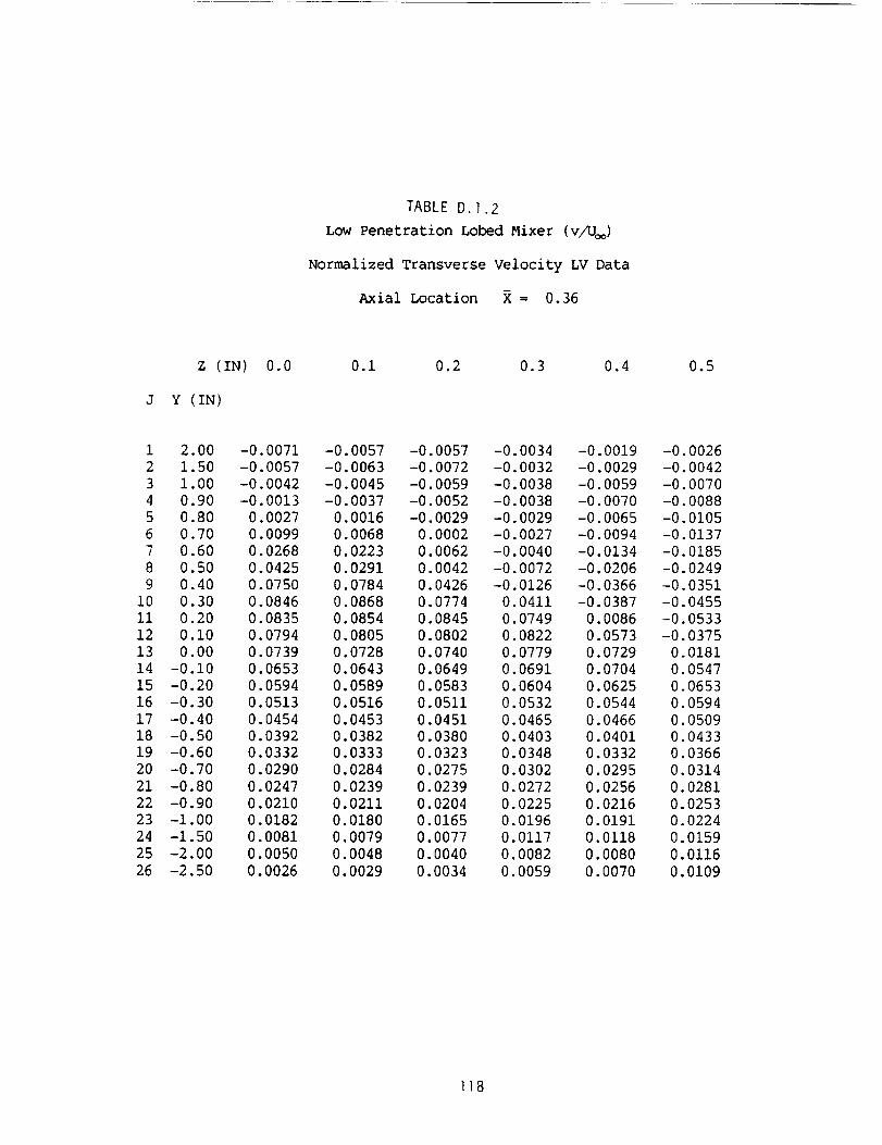
TABLEDI.2Low Penetration LobedMixer (v/U_)

Normalized Transverse Velocity LV Data

Axial Location X = 0.36

Z (IN) 0.0

J Y (IN)

0.i 0.2 0.3 0.4 0.5

1 2.00 -0.00712 1.50 -0.00573 1.00 -0.00424 0.90 -0.00135 0.80 0.00276 0.70 0.00997 0.60 0.02688 0.50 0.04259 0.40 0.0750

i0 0.30 0.0846Ii 0.20 0.083512 0.10 0.079413 0.00 0.073914 -0.i0 0.065315 -0.20 0.059416 -0.30 0.051317 -0.40 0.045418 -0.50 0.039219 -0.60 0.033220 -0.70 0.029021 -0.80 0.024722 -0.90 0.021023 -i.00 0.018224 -1.50 0.008125 -2.00 0.005026 -2.50 0.0026

-0.0057 -0.0057 -0.0034 -0.0019-0.0063 -0.0072 -0.0032 -0.0029-0.0045 -0.0059 -0.0038 -0.0059-0.0037 -0.0052 -0.0038 -0.00700.0016 -0.0029 -0.0029 -0.00650.0068 0.0002 -0.0027 -0.00940.0223 0.0062 -0.0040 -0.01340.0291 0.0042 -0.0072 -0.02060.0784 0.0426 -0.0126 -0.03660.0868 0.0774 0.0411 -0.03870.0854 0.0845 0.0749 0.00860.0805 0.0802 0.0822 0.05730.0728 0.0740 0.0779 0.07290.0643 0.0649 0.0691 0.07040.0589 0.0583 0.0604 0.06250.0516 0.0511 0.0532 0.05440.0453 0.0451 0.0465 0.04660.0382 0.0380 0.0403 0.04010.0333 0.0323 0.0348 0.03320.0284 0.0275 0.0302 0.02950.0239 0.0239 0.0272 0.02560.0211 0.0204 0.0225 0.02160.0180 0.0165 0.0196 0.01910.0079 0.0077 0.0117 0.01180.0048 0.0040 0.0082 0.00800.0029 0.0034 0.0059 0.0070

-0.0026-0.0042-0.0070-0.0088-0.0105-0.0137-0.0185-0.0249-0.0351-0.0455-0.0533-0.03750.01810.05470.06530.05940.05090.04330.03660.03140.02810.02530.02240.01590.01160.0109

118

TABLED.I.2 (Continu_d)

LowPenetration LobedMixer (v/U_)

Normalized Transverse Velocity LV Data

Axial Location X : 0.36

Z (IN) 0.6

J Y (IN)

0.7 0.8 C .9 1.0

1 2.00 -0.0047

2 1.50 -0.0055

3 1.00 -0.0102

4 0.90 -0.0124

5 0.80 -0.0151

6 0.70 -0.0182

7 0.60 -0.0232

8 0.50 -0.0293

9 0.40 -0.0363

i0 0.30 -0.0462

ii 0.20 -0.0554

12 0.i0 -0.0605

13 0.00 -0.0596

14 -0.i0 -0.0213

15 -0.20 0.0378

16 -0.30 0.0534

17 -0.40 0.0471

18 -0.50 0.0369

19 -0.60 0.0306

20 -0.70 0.0258

21 -0.80 0.0213

22 -0.90 0.0182

23 -1.00 0.0178

24 -1.50 0.0114

25 -2.00 0.0077

26 -2.50 0.0061

-0.0059 -0.0056 -0.(053 -0.0051

-0.0099 -0.0096 -0.C096 -0.0105

-0.0174 -0.0185 -0.(193 -0.0198

-0.0208 -0.0210 -0.(1230 -0.0228

-0.0232 -0.0264 -0.(>270 -0.0261

-0.0285 -0.0303 -0.[_317 -0.0313

-0.0336 -0.0361 -0.(!369 -0.0368

-0.0400 -0.0415 -0.0426 -0.0418

-0.0483 -0.0481 -0.(1482 -0.0500

-0.0552 -0.0554 -0.(,551 -0.0560

-0.0623 -0.0624 -0.0627 -0.0634

-0.0723 -0.0684 -0.0693 -0.0692

-0.0808 -0.0788 -0.(i749 -0.0738

-0.0753 -0.0847 -0.(1838 -0.0838

-0.0460 -0.0857 -0.()872 -0.0856

0.0179 -0.0651 -0.(}872 -0.0912

0.0381 0.0100 -0.(_693 -0.0787

0.0284 0.0196 0.(!071 -0.0076

0.0203 0.0094 -0.(!022 -0.0108

0.0154 0.0091 0.0019 0.0001

0.0132 0.0090 0.(1048 0.0028

0.0116 0.0076 0.0060 0.0046

0.0105 0.0074 0.0055 0.0056

0.0058 0.0050 0.0055 0.0059

0.0042 0.0028 0.0047 0.0039

0.0034 0.0015 0.0027 0.0041

119

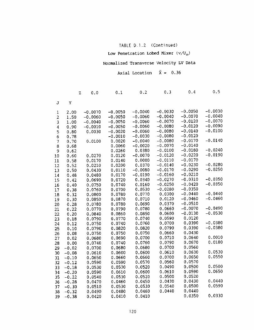
TABLED.I.2 (Continued)

Low Penetration Lobed Mixer (v/Um)

Normalized Transverse Velocity LV Data

Axial Location X = 0.36

J

1

2

3

4

5

6

7

8

9

I0

ii

12

13

14

15

16

17

18

19

2O

21

22

23

24

25

26

27

28

29

30

31

32

33

34

35

36

37

38

39

Y

2.00

1.50

1.00

0.90

0.80

0.78

0.70

0.68

0.62

0.60

0.58

0.52

0.50

0.48

0.42

0.40

0.38

0.32

0.30

0.28

0.22

0.20

0.18

0.12

0.i0

0.08

0.02

0.00

-0.02

-0.08

-0.10

-0.12

-0.18

-0.20

-0.22

-0.28

-0.30

-0.32

-0.38

Z 0.0

-0.0070

-0.0060

-0.0O40

-0.0010

0.0030

0.0100

0.0270

0.0170

0.0210

0.0430

O.048O

0.0690

0.0750

0.0760

0.0800

0.0850

0.0780

0.0770

0.0840

0.0790

0.0750

0.0790

0.0750

O.O68O

0.0740

0.0700

0.0610

0.0650

0.0590

0.0530

0.0590

0.0540

0.0470

0.0510

0.0490

0.0420

0.i 0.2 0.3 0.4 0.5

-0.0050 -0.0040 -0.0030

-0.0050 -0.0060 -0.0040

-0.0050 -0.0060 -0.0070

-0.0050 -0.0060 -0.0080

-0.0020 -0.0060 -0.0080

-0.0010 -0.0030 -0.0080

0.0020 -0.0040 -0.0080

0.0060 -0.0020 -0.0070

0.0260 0.0380 -0.0100

0.0120 -0.0070 -0.0120

0.0140 0.0000 -0.0110

0.0200 0.0370 -0.0140

0.0110 -0.0080 -0.0170

0.0170 -0.0190 -0.0160

0.0720 0.0340 -0.0270

0.0740 0.0160 -0.0250

0.0700 0.0530 -0.0280

0.0780 0.0770 0.0300

0.0870 0.0710 0.0120

0.0780 0.0690 0.0370

0.0790 0.0780 0.0660

0.0860 0.0850 0.0600

0.0770 0.0740 0.0590

0.0740 0.0760 0.0700

0.0820 0.0820 0.0790

0.0750 0.0750 0.0660

0.0690 0.0700 0.0710

0.0740 0.0760 0.0790

0.0680 0.0680 0.0700

0.0600 0.0600 0.0610

0.0660 0.0660 0.0700

0.0590 0.0570 0.0560

0.0530 0.0520 0.0490

0.0610 0.0600 0.0610

0.0530 0.0520 0.0500

0.0460 0.0450 0.0430

0.0530 0.0530 0.0540

0.0480 0.0460 0.0440

0.0410 0.0410

-0.0050

-0.0070

-0.0120

-0.0120

-0.0140

-0.0120

-0.0170

-0.0140

-0.0180

-0.0220

-0.0170

-0.0230

-0.0290

-0.0210

-0.0310

-0.0420

-0.0350

-0.0440

-0.0460

-0.0510

-0.0070

-0.0130

0.0120

0 0390

0 0390

0 0430

0 0640

0 0670

0 0560

0 0630

0.0650

O.057O

0.0500

0.0590

0.0520

0.0430

0.0500

0.0440

0.0350

-0.0030

-0.0040

-0.0070

-0.0090

-0.0100

-0.0140

-0.0240

-0.0190

-0.0280

-0.0250

-0.0350

-0.0350

-0.0440

-0.0460

-0.0490

-0.0530

-0.0380

-0.O38O

0.0010

0.0180

0.0530

0.0550

0.0500

0.0650

0.0440

0.0590

0.0330

120

TABLE D.].2 (Continued)

Low Penetration Lobed Mixer (v/U=)

Normalized Transverse Velocity LV Data

Axial Location K = 0.36

(Continuedi

J

40

41

42

43

44

45

46

47

48

49

50

51

52

53

54

55

56

Y

-0.40

-0.42

-0.48

-0.50

-0.52

-0.58

-0.60

-0.62

-0.68

-0.70

-0.78

-0.80

-0.90

-i.00

-i. 50

-2.00

-2.50

Z 0.0

0.0450

0.0450

0.0380

0.0390

0.0390

0.0320

0.0330

0.0350

0.0280

0.0290

0.0240

0.0250

0.0210

0.0180

0.0080

0.0050

0.0030

0.i 0.2 0.3 0.4 0.5

0.0460 0.0460 0.0470 0.0410

0.0440 0.0410 0.0410 0.0380

0.0370 0.0360 0.0300

0.0400 0.0400 0.0400 0.0340

0.0380 0.0360 0.0330 0.0310

0.0320 0.0310 0.0250

0.0350 0.0340 0.0340 0.0280

0.0340 0.0320 0.0300 0.0260

0.0290 0.0270 0.0210

0.0300 0.0290 0.0290 0.0240

0.0240 0.0220 0.0170 0.0180

0.0250 0.0250 0.0230 0.0200

0.0220 0.0200 0.0210 0.0170

0.0180 0.0180 0.0170 0.0140

0.0090 0.0090 0.0100 0.0090

0.0050 0.0050 0.0060 0.0070

0.0030 0.0030 0.0060 0.0070

0.0510

0.0260

0.0430

0.0220

0.0370

0.0180

0.0310

0.0150

0.0280

0.0250

0.0220

0.0160

0.0120

0.0110

121

TABLED.1.3

Low Penetration Lobed Mixer (w/U=)

Normalized Spanwise Velocity LV Data

Axial Location X = 0.36

Y

Z 0.0 0.1 0.2 0.3 0.4 0.5

1

2

3

4

5

6

7

8

0.00 0.0000 -0.0010 -0.0050 -0.0110 -0.0120 0.0000

0.i0 0.0010 -0.0010 -0.0100 -0.0140 -0.0020 0.0060

0.20 0.0000 -0.0040 -0.0080 -0.0030 0.0080 0.0120

0.30 0.0020 -0.0010 -0.0040 0.0060 0.0170 0.0180

0.40 0.0000 0.0010 -0.0040 0.0230 0.0250 0.0200

0.50 0.0000 0.0130 0.0270 0.0300 0.0230 0.0200

0.60 0.0010 0.0120 0.0230 0.0230 0.0210 0.0190

0.70 0.0000 0.0060 0.0120 0.0160 0.0150 0.0140

J Y

Z 0.6 0.7 0.8 0.9

1 0.00 0.0120 0.0110 0.0050 0.0010

2 0.i0 0.0140 0.0070 0.0020 0.0000

3 0.20 0.0120 0.0070 0.0030 0.0000

4 0.30 0.0130 0.0090 0.0060 0.0010

5 0.40 0.0150 0.0110 0.0080 0.0050

6 0.50 0.0150 0.0130 0.0080 0.0050

7 0.60 0.0160 0.0130 0.0100 0.0080

8 0.70 0.0130 0.0110 0.0080 0.0060

122

TABLE D.1.4

Low Penetration Lo_,d Mixer (PT)

Normalized Total Plessure Data

Axial Location X = 0.01

Z

Y

0.00 0.05 0.i0 0.15 0.20 0.25

1 0.70 0.9990 1.0000 1.0000 1.0000 1.0000 1.0000

2 0.60 0.9640 0.9670 0.9830 0.9940 0.9980 1.0000

3 0.50 0.3010 0.2870 0.2800 0.7270 0.8430 0.9290

4 0.40 0.5150 0.5070 0.4710 0.4160 0.3550 0.4400

5 0.30 0.6900 0.6810 0.6610 0.6210 0.5700 0.4900

6 0.20 0.8370 0.8180 0.8030 0.7790 0.7460 0.6930

7 0.i0 0.9500 0.9370 0.9260 0.9040 0.8840 0.8470

8 0.00 0.9940 0.9890 0.9850 0.9780 0.9690 0.9480

9 -0.i0 0.9990 0.9990 0.9990 0.9980 0.9970 0.9940

i0 -0.20 0.9990 0.9990 0.9990 0.9990 0.9990 0.9990

ii -0.30 0.9990 1.0000 1.0000 1.0000 1.0000 1.0000

12 -0.40 0.9990 0.9990 1.0000 0.9990 1.0000 0.9990

13 -0.50 0.9990 0.9990 1.0000 0.9990 1.0000 0.9990

14 -0.60 0.9990 0.9990 1.0000 0.9990 1.0000 0.9990

J

Z

Y

0.30 0.35 0.40 0.45 0.50

1 0.70

2 0.60

3 0.50

4 0.40

5 0.30

6 0.20

7 0.i0

8 0.00

9 -0.i0

i0 -0.20

ii -0.30

12 -0.40

13 -0.50

14 -0.60

1.0000 1.0000 1.0000 1.0000 1.0000

0.9990 0.9990 0.9990 0.9990

0.9760 0.9920 0.9970 0.9990 0.9990

0.7680 0.8940 0.9540 0.9850 0.9960

0.3770 0.5920 0.7440 0.8670 0.9410

0.6040 0.4880 0.1280 0.5920 0.7700

0.7830 0.6540 0.5690 0.1910 0.5330

0.9150 0.8520 0.7710 0.6460 0.4780

0.9850 0.9640 0.9170 0.8260 0.6740

0.9990 0.9960 0.9890 0.9640 0.8970

1.0000 1.0000 0.9990 0.9980 0.9890

1.0000 0.9990 0.9990 0.9990 0.9890

1.0000 0.9990 0.9990 0.9990 0.9890

1.0000 0.9990 0.9990 0.9990 0.9890

123

TABLE D.2.|

High Penetration Lobed Mixer, (u+U_)/U_

Normalized Axial Velocity LV Data

Axial Location X = 0.36

Y

Z 0.0 0.i 0.2 0.3 0.4 0.5

1 2.10

2 2.00

3 1.90

4 1.80

5 1.70

6 1.60

7 1.50

8 1.40

9 1.30

i0 1.20

ii 1.10

12 1.00

13 0.90

14 0.70

15 0.50

16 0.30

17 0.10

18 -0.i0

19 -0.30

20 -0.50

21 -0.70

22 -0.90

23 -1.00

24 -1.10

25 -1.20

26 -1.30

27 -1.40

28 -1.50

29 -1.60

30 -1.70

31 -1.80

32 -1.90

33 -2.00

34 -2.10

0.9820 0.9850 0.9880 0.9992 0.9960

0.4010 0.5020 0.9820 0.9890 0.9940

0.5310 0.4970 0.8460 0.9870 0.9920

0.6270 0.6170 0.6060 0.9900 0.9960

0.7110 0.7140 0.5440 0.9870 0.9930

0.7530 0.7530 0.6480 0.9790 0.9930

0.8110 0.8090 0.7360 0.8360 0.9910

0.8650 0.8640 0.8090 0.7080 0.9940

0.9080 0.9010 0.8570 0.6450 0.9890

0.9550 0.9490 0.9200 0.6560 0.9890

0.9740 0.9730 0.9540 0.7130 0.9840

0.9790 0.9770 0.9660 0.7810 0.9230

0.9820 0.9800 0.9740 0.9160 0.8360

0.9860 0.9850 0.9830 0.9730 0.7050

0.9940 0.9920 0.9900 0.9870 0.8060

1.0000 0.9980 0.9970 0.9930 0.9800

1.0000 1.0000 1.0000 0.9950 0.9880

1.0000 0.9950 0.9920 0.9850 0.9850

1.0000 0.9980 0.9960 0.9900 0.9870

1.0000 0.9980 0.9980 0.9930 0.9910

1.0000 1.0000 0.9990 0.9970 0.9940

1.0000 1.0000 1.0000 0.9970 0.9940

1.0000 1.0000 1.0000 1.0000 0.9960

1.0000 1.0000 1.0000 1.0000 0.9950

1.0000 1.0000 1.0000 1.0000 0.9980

1.0000 1.0000 1.0000 1.0000 0.9960

1.0000 1.0000 1.0000 1.0000 0.9990

1.0000 1.0000 1.0000 1.0000 1.0000

1.0000 1.0000 1.0000 1.0000 1.0000

1.0000 1.0000 1.0000 1.0000 1.0000

1.0000 1.0000 1.0000 1.0000 1.0000

1.0000 1.0000 1.0000 1.0000 1.0000

1.0000 1.0000 1.0000 1.0000 1.0000

1.0000 1.0000 1.0000 1.0000 1.0000

0.7840

0.8500

0.9770

0.9900

0.9910

0.9930

0.9930

0.9940

0.9930

0.9970

0.9970

0.9970

0.9970

0.9970

0.9980

0.9960

0.9980

]24

TABLED.2.2

High Penetration Lobed Mixe[ (v/U_)

Normalized Spanwise Velocity LV Data

Axial Location X = 0.36

Y

Z 0.6 0.7 0.8 0.9 1.0

1

2

3

4

5

6

7

8

9

i0

ii

12

13

14

15

16

17

18

19

2O

21

22

23

-2

-2

-i

-i

-I

-i

-i

-0

-0

-0

-0

-0

0

0

0

0

1

1

1

1

1

2

2

.2

.0

.8

.6

.4

.2

.0

.8

.6

.4

.2

.0

.2

.4

.6

.8

.0

.2

.4

.6

.8

.0

.2

0.0050

0.0280

0.0670

0.0910

0.1030

0.1170

0.1260

0.0850

0.0080

-0.0280

-0.1130

-0.2360

-0.2500

-0.2380

-0.2180

-0.2020

-0.1900

-0.1660

-0.1440

-0.1190

-0.0910

-0.0620

-0.0340

0.0210 -0.0460

0.0170 -0.0150

0.0830 0.0210

0.0960 -0.0630

0.0650 -0.2730

0.0210 -0.3100

-0.0610 -0.3280

-0.2170 -0.3150

-0.2930 -0.3030

-0.2940 -0.2930

-0.2830 -0.2830

-0.2690 -0.2670

-0.2520 -0.2510

-0.2350 -0.2350

-0.2180 -0.2180

-0.2010 -0.2010

-0.1840 -0.1820

-0.1640 -0.1610

-0.1410 .0.1470

-0.1160 -0.1170

-0.0910 -0.0930

-0.0660 -0.0690

-0.0470 -0.0560

-0 0610

-0 0920

-0 2750

-0 3200

-0 3240

-0 3210

-0 3180

-0 3040

-0 2940

-0 2840

-0 2730

-0 2580

-0.2420

-0.2280

-0.2100

-0.1970

-0.1750

-0.1550

-0.1330

-0.1090

-0.0870

-0.0660

-0.0480

-0.0740

-0.1520

-0.2810

-0.3120

-0.3120

-0.3150

-0.3130

-0.3020

-0.2920

-0.2820

-0.2720

-0.2590

-0.2440

-0.2320

-0.2120

-0.1990

-0.1780

-0.1560

-0.1340

-0.iii0

-0.0890

-0.0690

-0.0520

125

TA8LE D.2.3

High Penetration Lobed Mixer (w/U_)

Normalized Spanwise Velocity LV Data

Axial Location X = 0.36

J Y

Z 0.0 0.i 0.2 0.3 0.4 0.5

1

2

3

4

5

6

7

8

9

i0

ii

12

13

0.00

0.20

0.40

0.60

0.80

1.00

1.20

1.40

1.60

1.80

2.00

2.20

2.40

0.0020

0.0030

0.0040

0.0030

0.0040

0.0010

0.0030

-0.0010

-0.0030

0.0030

0.0200

0.0080

0.0030

-0.0030 -0.0100 -0.0190 -0.0390

-0.0020 -0.0100 -0.0080 -0.0490

-0.0010 -0.0080 -0.0620 -0.0280

-0.0020 -0.0080 -0.0400 0.0070

0.0010 -0.0070 -0.0650 0.0210

0.0060 -0.0020 -0.0660 0.0270

-0.0030 -0.0040 0.0140 0.0360

0.0000 -0.0310 0.0500 0.0390

-0.0040 -0.0170 0.0580 0.0460

-0.0010 0.0910 0.0760 0.0600

0.0100 0.1080 0.0880 0.0660

0.0060 0.0310 0.0390 0.0370

0.0030 0.0110 0.0170 0.0190

0.0050

0.0190

0.0200

0.0160

0.0180

0.0200

0.0270

0.0300

0.0360

0.0440

O.O52O

0.0330

0.0190

Y

Z 0.6 0.7 0.8 0.9 1.0

1

2

3

4

5

6

7

8

9

i0

ii

12

13

0.00 0.0040 0.0050 0.0000 -0.0020 0.0060

0.20 0.0140 0.0070 0.0010 -0.0030 0.0030

0.40 0.0120 0.0070 0.0010 -0.0030 0.0040

0.60 0.0100 0.0050 0.0000 -0.0040 0.0030

0.80 0.0120 0.0060 0.0010 -0.0040 0.0040

1.00 0.0140 0.0090 0.0030 -0.0040 0.0040

1.20 0.0200 0.0130 0.0040 -0.0030 0.0030

1.40 0.0220 0.0130 0.0050 -0.0030 0.0040

1.60 0.0250 0.0180 0.0080 -0.0030 0.0030

1.80 0.0340 0.0230 0.0110 0.0020 -0.0020

2.00 0.0380 0.0280 0.0190 0.0090 0.0000

2.20 0.0250 0.0190 0.0140 0.0040 0.0000

2.40 0.0160 0.0140 0.0110 0.0060 0.0000

126

TABLE D.2.4

High Penetration Lobed Mixer (PT)

Normalized Total Pressure Data

Axial Location X = 0.07

J Y

Z 0.0 0.i 0.2 0.3 0.4 0.5

1 2.20 1.0000 1.0000 1.0000 1.0000 1.0000 1.0000

2 2.10 1.0000 1.0000 1.0000 1.0000 1.0000 1.0000

3 2.00 0.1470 0.2030 1.0000 1.0000 1.0000 1.0000

4 1.90 0.2950 0.3590 0.9170 1.0000 1.0000 1.0000

5 1.80 0.4430 0.5080 0.0360 1.0000 1.0000 1.0000

6 1.70 0.5630 0.6320 0.3620 1.0000 1.0000 1.0000

7 1.60 0.6620 0.7320 0.5040 1.0000 1.0000 1.0000

8 1.50 0.7500 0.8190 0.6270 1.0000 1.0000 1.0000

9 1.40 0.8410 0.9050 0.7540 0.2830 1.0000 1.0000

i0 1.30 0.9400 0.9720 0.8660 0.0220 1.0000 1.0000

ii 1.20 0.9930 0.9950 0.9420 0.5470 1.0000 1.0000

12 i.i0 1.0000 1.0000 0.9790 0.6700 1.0000 1.0000

13 1.00 1.0000 1.0000 0.9930 0.7900 1.0000 1.0000

14 0.90 1.0000 1.0000 1.0000 0.9000 0.9750 1.0000

15 0.80 1.0000 1.0000 1.0000 0.9710 0.5380 1.0000

16 0.70 1.0000 1.0000 1.0000 1.0000 0.0000 1.0000

17 0.60 1.0000 1.0000 1.0000 1.0000 0.4020 1.0000

18 0.50 1.0000 1.0000 1.0000 1.0000 0.6680 1.0000

19 0.40 1.0000 1.0000 1.0000 1.0000 0.9450 1.0000

20 0.30 1.0000 1.0000 1.0000 1.0000 0.9520 0.9780

21 0.20 1.0000 1.0000 1.0000 1.0000 0.9930 0.7140

22 0.i0 1.0000 1.0000 1.0000 1.0000 1.0000 0.0220

23 0.00 1.0000 1.0000 1.0000 1.0000 1.0000 -0.0400

24 -0.i0 1.0000 1.0000 1.0000 1.0000 1.0000 -0.0400

25 -0.20 1.0000 1.0000 1.0000 1.0000 1.0000 0.7140

26 -0.30 1.0000 1.0000 1.0000 1.0000 1.0000 0.9890

27 -0.40 1.0000 1.0000 1.0000 1.0000 1.0000 1.0000

28 -0.50 1.0000 1.0000 1.0000 1.0000 1.0000 1.0000

29 -0.60 1.0000 1.0000 1.0000 1.0000 1.0000 1.0000

30 -0.80 1.0000 1.0000 1.0000 1.0000 1.0000 1.0000

31 -i.00 1.0000 1.0000 1.0000 1.0000 1.0000 1.0000

32 -1.50 1.0000 1.0000 1.0000 1.0000 1.0000 1.0000

33 -2.00 1.0000 1.0000 1.0000 1.0000 1.0000 1.0000

34 -2.50 1.0000 1.0000 1.0000 1.0000 1.0000 1.0000

_27

TABLE D.3.I

ADVANCED HIGH PENETRATION

Lobed Mixer (u+U_/U_)

Normalized Axial Velocity LV Data

Axial Location X = 0.05

Z

J Y

0.0 0.i 0.2 0.3 0.4 0.5

1 1.40

2 1.30

3 1.20

4 1 .I0

5 1.00

6 0.90

7 0.80

8 0.70

9 0.60

i0 0.50

ii 0.40

12 0.30

13 0.20

14 0.10

15 0.00

16 -0.I0

17 -0.20

18 -0.30

19 -0.40

20 -0.50

21 -0.60

22 -0.70

23 -0.80

24 -0.90

25 -i. 00

26 -i.i0

27 -i .20

28 -1.30

1.4862 1.5098 1.4853 1.4678 1.4280 1.3977

1.4937 1.5098 1.5170 1.5064 1.4963 1.4813

0.8334 0.6550 0.2084 1.4399 1.5064 1.4942

1.0074 1.1527 1.1828 0.7170 1.3338 1.5008

1.3215 1.3321 1.4209 1.2326 0.4931 1.4915

1.4303 1.4408 1.4680 1.3610 1.1013 1.0953

1.4783 1.4833 1.4851 1.4165 1.1767 0.7839

1.4809 1.4860 1.4864 1.4316 1.1800 0.7012

1.4788 1.4870 1.4872 1.4467 1.1956 0.6560

1.4775 1.4858 1.4861 1.4664 1.2045 0.6310

1.4789 1.4834 1.4844 1.4751 1.2308 0.6472

1.4771 1.4831 1.4878 1.4845 1.2216 0.6799

1.4627 1.4858 1.4875 1.4861 1.2446 0.6877

1.4796 1.4859 1.4895 1.4941 1.2761 0.7060

1.4817 1.4877 1.5059 1.4875 1.3168 0.7257

1.4799 1.4849 1.4909 1.4775 1.2997 0.7373

1.4788 1.4858 1.4908 1.4704 1.2850 0.7420

1.4799 1.4854 1.4903 1.4705 1.2547 0.7449

1.4742 1.4835 1.4875 1.4716 1.2504 0.7685

1.4723 1.4808 1.4849 1.4842 1.2569 0.7518

1.4669 1.4725 1.4825 1.4957 1.3025 0.7652

1.4549 1.4599 1.4781 1.4963 1.3626 0.6190

1.4335 1.4390 1.4579 1.4892 1.4326 0.9049

1.4108 1.4121 1.4411 1.4765 1.4924 0.9664

1.3694 1.3755 1.4015 1.4163 1.4935 1.4816

1.3188 1.3250 1.3503 1.4016 1.4618 0.8909

1.2357 1.2345 1.2752 1.3339 1.3937 1.3771

1.1019 1.1061 1.1475 1.2115 1.3554 1.3771

]28

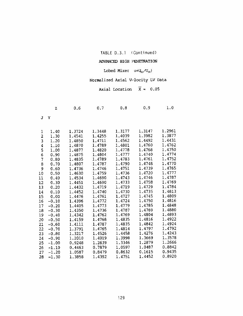
TABLE D.3.1 (Continued)

ADVANCED HIGH PENETRATION

Lobed Mixer u+U_/U_)

Normalized Axial W,locity LV Data

Axial Location X-- 0.05

Z

J Y

0.6 0.7 0.8 0.9 1.0

1

2

3

4

5

6

7

8

9

i0

ii

12

13

14

15

16

17

18

19

2O

21

22

23

24

25

26

27

28

1.40

1.30

1.20

i.i0

1.00

0.90

0.80

0.70

0.60

0.50

0.40

0.30

0.20

0.i0

0.00

-0. i0

-0.20

-0.30

-0.40

-0.50

-0.60

-0.70

-0.80

-0.90

-1.00

-I .10

-i. 20

-i. 30

1.3724

1.4541

1.4850

1.4870

1.4877

1.4875

1.4835

1.4807

1.4736

1.4630

1.4534

1.4451

1.4432

1.4452

1.4476

1.4396

1.4405

1.4350

1.4342

1.4159

1.4111

1.3791

1.3217

1.2010

0.9248

0.4463

1.0587

1.3858

1.3448 1.3177 1.3147

1.4255 1.4039 1.3982

1.4711 1.4562 1.4492

1.4789 1.4801 1.4760

1.4820 1.4778 1.4768

1.4804 1.4777 1.4740

1.4789 1.4783 1.4761

1.4787 1.4790 1.4748

1.4746 1.4751 1.4739

1.4759 1.4736 1.4720

1.4690 1.4743 1.4746

1.4690 1.4733 1.4758

1.4719 1.4719 1.4729

1.4740 1.4730 1.4735

1.4761 1.4727 1.4745

1.4772 1.4724 1.4750

1.4773 1.4779 1.4785

1.4736 1.4787 1.4769

1.4762 1.4769 1.4804

1.4768 1.4835 1.4816

1.4787 1.4835 1.4842

1.4765 1.4814 1.4797

1.4526 1.4458 1.4276

1.4019 1.3998 1.3669

1.2639 1.3346 1.2879

0.7879 1.0597 1.0487

0.8479 0.8632 0.1615

1.4392 1.4751 1.4452

1.2961

1.3877

1.4431

1.4762

1.4750

1.4774

1.4752

1.4770

1.4765

1.4777

1.4787

1.4769

1.4784

1.4813

1.4809

1.4816

1.4848

1.4880

1.4893

1.4922

1.4924

1.4792

1.4243

1.3578

1.2666

0.8842

0.9435

0.8920

129

TABLED.3.2

ADVANCED HIGH PENETRATION

Lobed Mixer (v/U_)

Normalized Transverse Velocity LV Data

Axial Location X -- 0.05

Z

J Y

0.0 0.I 0.2 0.3 0.4 0.5

i

2

3

4

5

6

7

8

9

i0

ii

12

13

14

15

16

17

18

19

20

21

22

23

24

25

26

27

28

1.34

1.30

1.20

i.i0

1.00

0.90

0.80

0.70

0.60

0.50

0.40

0.30

0.20

0.10

0.00

-0.i0

-0.20

-0.30

-0.40

-0.50

-0.60

-0.70

-0.80

-0.90

-i. O0

-i. i0

-i .20

-1.30

-0.0535

-0.0875

-0.0304

0.0046

0.0038

0.1114

0.0910

0.1010

0.1015

0.i010

0.1018

0.1018

0.1023

0.1036

0.1035

0.1032

0.1036

0.1040

0.1009

0.0980

0.0941

0.0860

0.0754

0.0643

0.0492

0.0266

0.0127

-0.0059

-0.0503 -0.0499 -0.0512 -0.0522

-0.0818 -0.0761 -0.0659 -0.0653

-0.0223 -0.0355 -0.1132 -0.0931

0.0295 0.0134 0.1900 -0.1448

0.0137 0.0077 0.1113 0.1060

0.0972 0.1028 0.1002 0.1484

0.1004 0.1066 0.1086 0.0484

0.1027 0.1031 0.1078 0.0712

0.1021 0.1021 0.1054 0.0574

0.1032 0.1014 0.1029 0.0651

0.1036 0.1008 0.1025 0.0735

0.1027 0.1009 0.1034 0.0790

0.1037 0.1017 0.1023 0.0825

0.1041 0.1025 0.i010 0.0753

0.1037 0.1035 0.1021 0.0798

0.1053 0.1044 0.1057 0.0821

0.1039 0.1063 0.1099 0.0787

0.1032 0.1058 0.1106 0.0778

0.1028 0.1048 0.1111 0.0919

0.0998 0.1006 0.1080 0.0965

0.0950 0.0960 0.1056 0.1075

0.0872 0.0899 0.1020 0.1218

0.0793 0.0820 0.0947 0.1279

0.0675 0.0696 0.0799 0.1119

0.0503 0.0490 0.0570 0.0785

0.0130 0.0176 0.0305 0.0272

0.0105 0.0048 0.0072 -0.0010

-0.0093 -0.0149 -0.0192 -0.0208

-0.0512

-0.0649

-0.0984

-0.1235

-0.1840

0.0182

0.0007

0.0122

-0.0018

0.0022

-0.0066

0.0097

0.0189

0.0235

0.0283

-0.0176

-0.0296

-0.0309

-0.0458

-0.0536

-0.0486

-0.0537

-0.0434

0.1019

0.1177

0.0358

-0.0031

-0.0379

l 30

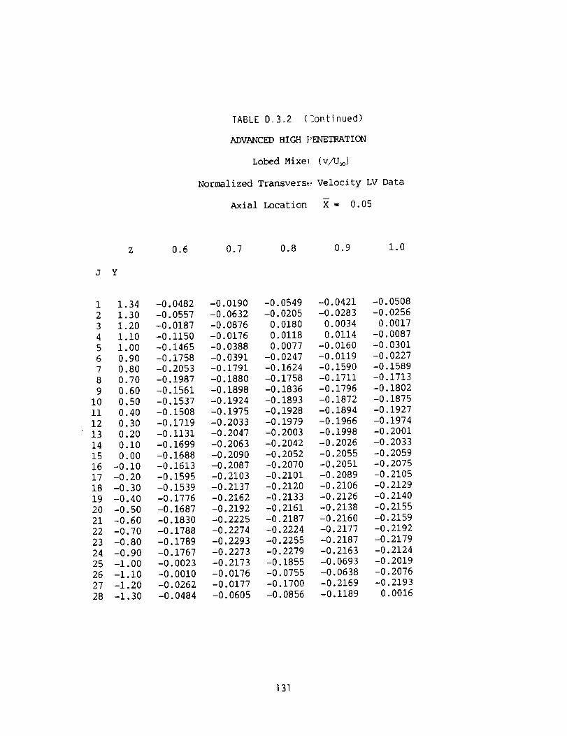
TABLED.3.2 (Continued)

ADVANCEDHIGHPENETRATION

LobedMixel (v/U=)

Normalized Transvers_ Velocity LV Data

Axial Location X = 0.05

Z

J Y

0.6 0.7 0.8 0.9 1.0

1 1.34 -0.0482 -0.0190 -0.0549 -0.0421

2 1.30 -0.0557 -0.0632 -0.0205 -0.0283

3 1.20 -0.0187 -0.0876 0.0180 0.0034

4 i.i0 -0.1150 -0.0176 0.0118 0.0114

5 1.00 -0.1465 -0.0388 0.0077 -0.0160

6 0.90 -0.1758 -0.0391 -0.0247 -0.0119

7 0.80 -0.2053 -0.1791 -0.1624 -0.1590

8 0.70 -0.1987 -0.1880 -0.1758 -0.1711

9 0.60 -0.1561 -0.1898 -0.1836 -0.1796

i0 0.50 -0.1537 -0.1924 -0.1893 -0.1872

ii 0.40 -0.1508 -0.1975 -0.1928 -0.1894

12 0.30 -0.1719 -0.2033 -0.1979 -0.1966

13 0.20 -0.1131 -0.2047 -0.2003 -0.1998

14 0.i0 -0.1699 -0.2063 -0.2042 -0.2026

15 0.00 -0.1688 -0.2090 -0.2052 -0.2055

16 -0.i0 -0.1613 -0.2087 -0.2070 -0.2051

17 -0.20 -0.1595 -0.2103 -0.2101 -0.2089

18 -0.30 -0.1539 -0.2137 -0.2120 -0.2106

19 -0.40 -0.1776 -0.2162 -0.2133 -0.2126

20 -0.50 -0.1687 -0.2192 -0.2161 -0.2138

21 -0.60 -0.1830 -0.2225 -0.2187 -0.2160

22 -0.70 -0.1788 -0.2274 -0.2224 -0.2177

23 -0.80 -0.1789 -0.2293 -0.2255 -0.2187

24 -0.90 -0.1767 -0.2273 -0.2279 -0.2163

25 -i.00 -0.0023 -0.2173 -0.1855 -0.0693

26 -1.10 -0.0010 -0.0176 -0.0755 -0.0638

27 -1.20 -0.0262 -0.0177 -0.1700 -0.2169

28 -1.30 -0.0484 -0.0605 -0.0856 -0.1189

-0.0508

-0.0256

0.0017

-0.0087

-0.0301

-0.0227

-0.1589

-0.1713

-0.1802

-0.1875

-0.1927

-0.1974

-0.2001

-0.2033

-0.2059

-0.2075

-0.2105

-0 2129

-0 2140

-0 2155

-0 2159

-02192

-02179

-0.2124

-0.2019

-0.2076

-0.2193

0.0016

131

Table D.3.3 (Continued)

ADVANCED HIGH PENETRATION

Lobed Mixer (w/U_)

Normalized Spanwise Velocity LV Data

Axial Location X = 0.05

Z (IN)

J Y (IN)

0.07 0.17 0.27 0.37 0.47

1

2

3

4

5

6

7

8

9

i0

ii

12

13

14

15

16

17

18

19

20

21

22

23

24

25

26

27

28

1.40

1.30

1.20

i.i0

1.00

0.90

0.80

0.70

0.60

0.50

0.40

0.30

0.20

0.i0

0.00

-0. i0

-0.20

-0.30-0.40

-0.50

-0.60

-0.70

-0.80

-0.90

-i. 00

-i.i0

-i. 20

-i. 30

0.0028

0.0001

-0.0089

-0.0097

-0.0057

-O.O05O

-0.0016

0.0026

-0.0011

-0.0017

-0.0026

-0.0028

-0.0008

-0.0004

0.0002

-0.0033-0.0027

-0.0027

-0.0034

-0.0072

-0.0031

-O.0108-0.0157

-0.0179-0.0174

-0.0215

-0.0228

-0.0355

0.0157 0.0233 0.0271 0.0285

0.0158 0.0271 0.0375 0.0349

-0.0079 -0.0251 0.0323 0.0370

0.0159 0.0660 0.2186 0.0048

0.0088 0.0469 0.1004 -0.1818

0.0172 0.0346 0.0771 0.1912

0.0180 0.0345 0.0737 0.1745

0.0185 0.0318 0.0614 0.1453

0.0120 0.0268 0.0657 0.1454

0.0157 0.0243 0.0527 0.1344

0.0138 0.0251 0.0606 0.1571

0.0157 0.0231 0.0549 0.1478

0.0151 0.0253 0.0614 0.1574

0.0121 0.0256 0.0641 0.1453

0.0146 0.0292 0.0654 0.1066

0.0143 0.0253 0.0654 0.1589

0.0086 0.0222 0.0525 0.1471

0.0116 0.0201 0.0580 0.1609

0.0057 0.0173 0.0491 0.1069

0.0050 0.0094 0.0513 0.1795

-0.0010 0.0037 0.0336 0.1305

-0.0057 -0.0061 0.0220 0.1056

-0.0124 -0.0150 -0.0065 0.0295

-0.0230 -0.0271 -0.0373 -0.0594

-0.0323 -0.0423 -0.0528 -0.0751

-0.0357 -0.0506 -0.0647 -0.0853

-0.0498 -0.0574 -0.0734 -0.0807

-0.0578 -0.0655 -0.0804 -0.0912

132

Table D.3.3 (Continued)

ADVANCED HIGH PENE_I_ATION

Lobed Mixer (w/U_)

Normalized Spanwise Vel(_city LV Data

Axial Location X -- 0.05

Z (IN) 0.57

J Y (IN)

0.67 0.77 0.87 0.97

1 1.40 0.0171

2 1.30 0.0253

3 1.20 0.0271

4 i.i0 0.0230

5 1.00 0.0032

6 0.90 -0.0302

7 0.80 -0.0662

8 0.70 -0.0917

9 0.60 -0.1084

i0 0.50 -0.1207

ii 0.40 -0.1236

12 0.30 -0.1243

13 0.20 -0.1193

14 0.10 -0.1064

15 0.00 -0.1158

16 -0.i0 -0.1198

17 -0.20 -0.1114

18 -0.30 -0.1131

19 -0.40 -0.1093

20 -0.50 -0.1151

21 -0.60 -0.1132

22 -0.70 -0.0997

23 -0.80 -0.0962

24 -0.90 -0.0753

25 -1.00 -0.0460

26 -i.i0 -0.1147

27 -1.20 -0.0890

28 -1.30 -0.0865

0.0142 0.0080

0.0231 0.0153

0.0217 0.0165

0.0176 0.0168

0.0097 0.0122

-0.0022 0.0072

-0.0247 -0.0034

-0.0360 -0.0133

-0.0468 -0.0180

-0.0496 -0.0226

-0.0515 -0.0241

-0.0544 -0.0270

-0.0518 -0.0291

-0.0517 -0.0277

-0.0560 -0.0300

-0.0588 -0.0288

-0.0647 -0.0290

-0.0619 -0.0312

-0.0621 -0.0330

-0.0619 -0.0316

-0.0562 -0.0319

-0.0518 -0.0316

-0.0548 -0.0333

-0.0574 -0.0317

-0.0564 -0.0428

-0.1478 -0.0599

-0.0998 -0.0978

-0.0910 -0.0675

-0.0019

0.0012

0.0079

0.0093

0.0100

0.0028

0.0028

-0.0007

-0.0063

-0.0088

-0.0104

-0.0122

-0.0124

-0 0180

-0 0157

-0 0153

-0 0186

-0 0194

-0 0190

-0 0191

-0 0193

-0.0244

-0.0247

-0.0229

-0.0173

-0.0321

-0.2672

-0.0308

-0.0056

-0.0070

-0.0004

0.0035

0.0029

O.O02O

0.0033

0.0018

0.0002

-0.0004

-0.0015

-0.0031

-0.0029

-0.0016

-0.0031

-0.0021

-0.0006

-0.0031

-O.OO25

-0.0055

-0.0031

-0.0061

-0.0101

-0.0039

-0.0193

-0.0349

-0.2096

-0.0186

133

TABLE D.3.4

ADVANCED HIGH PENETRATION

Lobed Mixer (PT/PT_)

Normalized Total Pressure Data

Axial Location X = 0.05

Y

K Z

0.0 -0.i -0.2 -0.3 -0.4 -0.5

1

2

3

4

5

6

7

8

9

i0

Ii

12

13

14

15

16

17

18

19

2O

21

1.00

0.90

0.80

0.70

0.60

0.55

0.53

0.51

0.50

0.49

0.47

0.45

0.43

0.41

0.40

0.39

0.37

0.30

0.20

0.10

0.00

0.9987

0.9987

0.9991

0.9989

0.9050

0.6994

0.6593

0.6199

0.5079

0.4329

0.5887

0.6774

0.7121

0.7381

0.7668

0.7973

0.8991

0.9868

0.9962

0.9965

0.9961

0.9986 0.9981 0.9977

0.9986 0.9984 0.9976

0.9988 0.9984 0.9977

0.9987 0.9984 0.9974

0.8968 0.8851 0.8706

0.6942 0.6894 0.6840

0.6546 0.6495 0.6468

0.6173 0.6145 0.6091

0.4912 0.4953 0.5054

0.4241 0.3937 0.4004

0.5898 0.5692 0.5610

0.6788 0.6630 0.6457

0.7091 0.6956 0.6769

0.7388 0.7183 0.7018

0.7643 0.7451 0.7277

0.7893 0.7701 0.7563

0.8852 0.8666 0.8629

0.9823 0.9787 0.9784

0.9955 0.9932 0.9898

0.9951 0.9927 0.9887

0.9953 0.9923 0.9889

0.9977

0.9977

0.9982

0.9969

0.8480

0.6646

0.6300

0.5975

0.4537

0.3815

0.5639

0.6417

0.6664

0.6954

0.7230

0.7529

0.8784

0.9802

0.9857

0.9839

0.9840

0.9972

0.9974

0.9975

0.9958

0.8437

0.6725

0.6353

0.6000

0.4569

0.3802

0.5620

0.6465

0.6718

0.7023

0.7365

0.7714

0.9015

0.9801

0.9793

0.9779

0.9776

134

TABLED.3.4 (Coltinued)

ADVANCED HIGH PE4ETRATION

Lobed Mixer (?T/PT_)

Normalized Total Pressure Data

Axial Location X = 0.05

Y

K Z

-0.6 -0.7 -0.8 -0.9 -i.0 -i.i

1 1.00 0.9980

2 0.90 0.9985

3 0.80 0.9983

4 0.70 0.9944

5 0.60 0.8608

6 0.55 0.6936

7 0.53 0.6542

8 0.51 0.6207

9 0.50 0.4352

i0 0.49 0.4292

Ii 0.47 0.5902

12 0.45 0.6638

13 0.43 0.6938

14 0.41 0.7311

15 0.40 0.7671

16 0.39 0.8079

17 0.37 0.9325

18 0.30 0.9800

19 0.20 0.9744

20 0.I0 0.9695

21 0.00 0.9696

0.9826 0.9186 0.8438

0.9850 0.9306 0.8678

0.9882 0.9460 0.8956

0.9771 0.9369 0.8684

0.7765 0.7318 0.6543

0.6189 0.5891 0.4271

0.5881 0.5594 0.3361

0.5586 0.4616 0.5633

0.3777 0.3772 0.7214

0.4726 0.5828 0.7829

0.6285 0.6736 0.8222

0.6977 0.7340 0.8663

0.7326 0.7949 0.8978

0.7767 0.8370 0.9239

0.8160 0.8727 0.9419

0.8561 0.9040 0.9527

0.9534 0.9667 0.9651

0.9733 0.9606 0.9417

0.9617 0.9470 0.9217

0.9550 0.9384 0.9121

0.9580 0.9401 0.9120

0.7621

0.7982

0.8212

0.7338

0.5186

0.7953

0.8719

0.9233

0.9376

0.9525

0.9636

0.9642

0.9597

0.9549

0.9473

0.9470

0.9403

0.9141

0.8911

0.8808

0.8784

0.6152

0.6466

0.6246

0.5229

0.8779

0.9528

0.9586

0.9587

0.9551

0.9544

0.9478

0.9387

0.9306

0.9200

0.9153

0.9084

0.9039

0.8775

0.8492

0.8365

0.8385

135

TABLE D.3.4 (Continued)

ADVANCED HIGH PENETRATION

Lobed Mixer (PT/PT_)

Normalized Total Pressure Data

Axial Location X = 0.05

Y

K Z

0.00 0.i0 0.20 0.30 0.40 0.50

1

2

3

4

5

6

7

8

9

i0

ii

12

13

14

15

16

17

18

19

20

21

22

23

0.00

0.i0

0.20

0.30

0.35

0.38

0.40

0.41

0.42

0.43

0.44

0.45

0.46

0.47

0.48

0.49

0.50

0.55

0.60

0.70

0.80

0.90

1.00

0.9964

0.9967

0.9966

0.9879

0.9718

0.9425

0.9002

0.8810

0.8678

0.8487

0.7755

0.7436

0.7586

0.8492

0.8660

0.8821

0.8994

0.9764

0.9981

0.9971

0.9974

0.9978

0.9974

0.9973 0.9978 0.9982

0.9974 0.9976 0.9989

0.9977 0.9985 0.9993

0.9952 0.9976 0.9986

0.9835 0.9905 0.9886

0.9494 0.9521 0.9462

0.8887 0.8927 0.8890

0.8697 0.8805 0.8768

0.8550 0.8682 0.8650

0.8305 0.8552 0.8521

0.7875 0.8392 0.8385

0.6686 0.7901 0.7836

0.6901 0.7523 0.7588

0.8262 0.7641 0.7654

0.8433 0.8357 0.8375

0.8638 0.8637 0.8624

0.8764 0.8829 0.8824

0.9630 0.9716 0.9729

0.9977 0.9997 0.9989

0.9981 1.0000 0.9991

0.9987 1.0002 0.9989

0.9990 1.0008 0.9993

0.9992 1.0008 0.9994

1.0003

0.9997

0.9995

0.9989

0.9894

0.9474

0.8911

0.8783

0.8673

0.8542

0.8421

0.8173

0.7466

0.7554

0.8172

0.8544

0.8766

0.9713

0.9983

0.9997

0.9990

0.9982

0.9986

1.0135

1.0126

1.0119

1.0121

0.9978

0.9505

0.8921

0.8814

0.8695

0.8561

0.8434

0.8220

0.7507

0.7461

0.7827

0.8493

0.8766

0.9865

1.0118

1.0117

1.0123

1.0121

1.0123

136

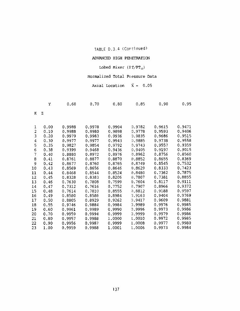
TABLE D.3.4 (Cop[inued)

ADVANCED HIGH PENETRATION

Lobed Mixer (FT/PT=_)

Normalized Total P[essure Data

Axial Location _ = 0.05

Y

K Z

0.60 0.70 0.80 0.85 0.90 0.95

1

2

3

4

5

6

7

8

9

I0

ii

12

13

14

15

16

17

18

19

2O

21

22

23

0.00

0 .i0

0.20

0.30

0.35

0.38

0.40

0.41

0.42

0.43

0.44

0.45

0.46

0.47

0.48

0.49

0.50

0.55

0.60

0.70

0.80

0.90

1.00

0.9988

0.9988

0.9979

0.9977

0.9827

0.9399

0.8880

0.8761

0.8677

0.8569

0.8468

0.8328

0.7630

0.7312

0.7614

0.8580

0.8805

0.9746

0.9961

0.9959

0.9957

0.9956

0.9959

0.9978

0.9980

0.9983

0.9977

0.9854

0.9468

0.8972

0.8877

0.8760

0.8656

0.8544

0.8383

0.7808

0.7616

0.7810

0.8586

0.8929

0.9884

0.9989

0.9994

0.9988

0.9987

0.9988

0.9904

0.9898

0.9936

0.9943

0.9792

0.9436

0.8976

0.8870

0.8765

0.8646

0.8524

0.8206

0.7599

0.7752

0.8555

0.8984

0 9262

0 9984

0 9990

0 9999

1 0000

0 9999

1.0001

0.9782

3.9778

3.9835

3.9885

13.9743

13.9405

0.8962

0.8852

0.8749

0.8629

0.8480

i).7807

0.7604

0.7907

i).8812

0.9163

0.9417

0.9989

c).9996

0.9999

L.0010

L.0008

[.0006

0.9615

0.9593

0.9686

0.9738

0.9557

0.9197

0.8756

0.8655

0.8545

0.8333

0.7362

0.7381

0.8117

0.8966

0 9188

0 9404

0 9609

0 9976

0 9973

0 9979

0 9972

0.9977

0.9973

0.9471

0.9406

0.9515

0.9558

0.9359

0.9015

0.8560

0.8369

0.7532

0.7423

0.7875

0.8855

0.9111

0.9372

0.9597

0.9769

0.9881

0.9985

0.9986

0.9986

0.9985

0.9980

0.9984

137

TABLED.3.4 (Continued)

ADVANCED HIGH PENETRATION

Lobed Mixer (PT/PT_)

Normalized Total Pressure Data

Axial Location X = 0.05

Y

K Z

1.00 1.05

1

2

3

4

5

6

7

8

9

i0

ii

12

13

14

15

16

17

18

19

20

21

22

23

0.00

0.i0

0.20

0.30

0.35

0.38

0.40

0.41

0.42

0.43

0.44

O.45

0.46

0.47

0.48

0.49

0.50

0.55

0.60

0.70

0.80

0.90

1.00

0.9322

0.9208

0.9326

0.9333

0.9108

0.8762

0.8657

0.8539

O.8400

0.7581

0.7374

0.7554

0.8643

0.9044

0.9242

0.9503

0.9673

0.9830

0.9982

0.9983

0.9984

0.9980

0.9987

0.9181

0.8982

0.9093

0.9038

0.8774

0.8574

0.7498

0.7302

0.7501

0.8677

0.9029

0.9241

0.9456

0.9635

0.9790

0.9882

0.9958

1.0001

0.9997

0.9998

0.9996

1.0003

1.0000

]38

TABLE D. 4

SINUSOIDAL LOBE[, MIXERS

LOBE TRAILING EDGE LOUNDARY LAYER

LOW PENETRATION

CREST OUTER

Z = 0.0 Y = 0.5

CREST INNER

Z = 0.0 Y = 0.5

I NORMAL U / U_

1 0.02 0.327

2 0.04 0.417

3 0.07 0.814

4 0.12 0.968

5 0.15 0.982

6 0.200 0.999

NORMAL U / U_

1 0.03 0.625

2 0.08 0.703

3 0.18 0.822

4 0.28 0.899

5 0.38 0.956

6 0.48 0.990

7 0.58 0.996

8 0.68 0.997

9 0.78 0.997

i0 0.88 0.999

ii 0.98 1.000

FLAT PLATE

PARAMETER INLET EXIT

;REST EXIT

OUTER LOW

CREST_IT

I_RLOW

6" = 0.024

: 0.017

H = 1.41

6 = 0.145

= 0.04

= 0. 021

= 2.29

= 0.15

= 0. 0867

= 0.0587

: 1.48

= 0.48

139

TABLE0.4 (Continued)

SINUSOIDAL LOBED MIXERS

LOBE TRAILING EDGE BOUNDARY LAYER

HIGH PENETRATION

CREST OUTER

Z = 0.0 Y = 2.0

CREST INNER

7,= 0.0 Y = 2.0

I NORMAL U / U_ I NORMAL U / Uc_

1 0.025 0.650

2 0.050 0.800

3 0.075 0.940

4 0.i00 0.982

5 0.125 0.990

FLAT PLATE

PARAMETER INLET EXIT

1

2

3

4

5

6

7

8

9

i0

ii

12

13

14

15

CREST EXIT

OUTER HIGH

00

00

00

O.

O.

O.O.

i.1.

i.i.

I.

05 0.466

i0 0.531

20 0.627

30 0.711

40 0.753

50 0.811

60 0.865

70 0.908

80 0.955

90 0.974

00 0.979

i0 0.982

30 0.986

50 0.994

70 1.000

CREST EXIT

INNER HIGH

6_ = 0.039 = 0.0280

@ = 0.028 = 0.0146

H = 1.39 = 1.92

6 = 0.240 = 0.125

= 0.235

= 0.148

= 1.59

= 1.40

140

TABLED.4 (Continued)ADVANCED HIGH PENETRATION MI;CER

TRAILING EDGE BOUNDARY LAYI_R

3

4

5

6

7

8

9

i0

_W

0

H

6

Z=0.0

NORMAL

OUT

Y = 1.22

PT/PTo o

2 OUT

Z = 0.053 Y = 0 75

I NORMAL PT/PT_ o I

0.010 0.578 1 0.010 0.5(i2

0.016 0.702 2 0.015 0.6_i0

0.020 0.752 3 0.020 0.681

0.024 0.795 4 0.026 0.7_2

0.028 0.835 5 0.030 0.767

0.034 0.891 6 0.036 0.8G9

0.042 0.950 7 0.040 0.848

0.050 0.984 8 0.046 0.884

0.058 0.997 9 0.050 0.916

0.066 1.000 i0 0.056 0.944

ii 0.060 0.964

12 0.070 0.991

13 0.080 1.000

= 0.0098

= 0.0055

= 1.78

= 0.049

= 0. 0118

= 0. 0071

= 1.65

= 0.056

3 OUT

Z = 0.053 Y = 0.0

NORMAL PT/PTco

1 0.010 0.603

2 0.020 0.665

3 0.030 0.738

4 0.040 0.792

5 0.050 0.840

6 0.060 0.885

7 0.070 0.926

8 0.080 0.957

9 0.090 0.980

i0 0.i00 0.992

ii 0.ii0 0.996

12 0.160 1.000

= 0.0138

= 0.0091

= 1.52

= 0.090

4 OUT

Z = 0.053 Y = -0.75 Z

5 OUT

= 1.000 Y = -1.22

I NORMAL PT/'PT_ I NORMAL PT/'P'?_

1 0.010 0.500 1 0.010 0.339

2 0.020 0.582 2 0.030 0.45_

3 0.030 0.626 3 0.050 0.51;'

4 0.050 0.700 4 0.070 0.566

5 0.070 0.775 5 0.090 0.610

6 0.ii0 0.890 6 0.110 0.65_

7 0.160 0.964 7 0.130 0.686

8 0.210 0.989 8 0.150 0.71!1!

9 0.260 0.984 9 0.170 0.745

10 0.310 0.976 10 0.190 0.77!_

ii 0.360 0.969 ii 0.210 0.787

12 0.410 0.960 12 0.260 0.82_!I

13 0.450 0.951 13 0.310 0.86(!,

14 0.410 0.940

15 0.510 0.99_!:

16 0.610 1.00(

= 0.0283

= 0.0214

= 1.32

= (undefined)

O

H

6

= 0.0_ 52

= 0.0489

= 1.33

= 0.475

141

6OUT

Z = 0.000 Y = 1.59

I NORMAL PT/PT

1 0.010 0.548

2 0.020 0.626

3 0.030 0.684

4 0.042 0.743

5 0.050 0.772

6 0.062 0.822

7 0.070 0.846

8 0.080 0.872

9 0.090 0.893

10 0.100 0.919

ii 0.ii0 0.933

12 0.150 0.982

13 0.190 0.999

: 0.0187

= 0.0130

= 1.44

= 0.150

TABLE D.4 (Continued

ADVANCED HIGH PENETRATION MIXER

TRAILING EDGE BOUNDARY LAYER

i IN

Z = 0.0 Y = 1.16

2 IN

Z = 0.47 Y = 0.69

3 IN

Z = 0.47 Y = 0.0

NORMAL PT/PT_ I NORMAL PT/PT_

1 0.010 0.590 1 0.010 0.543

2 0.030 0.617 2 0.030 0.638

3 0.050 0.644 3 0.050 0.697

4 0.070 0.669 4 0.070 0.748

5 0.090 0.689 5 0.090 0.797

6 0.110 0.743 6 0.ii0 0.841

7 0.130 0.755 7 0.160 0.931

8 0.150 0.789 8 0.210 0.987

9 0.170 0.808 9 0.260 0.998

i0 0.190 0.837 i0 0.310 1.000

ii 0.210 0.860

12 0.310 0.968

13 0.410 1.000

= 0.0411

= 0.0322

= 1.28

= 0.348

6 )$

8

H

6

= 0.0262

= 0.0193

= 1.36

= 0.203

NORMAL PT/PT_

1 0.010 0.510

2 0.020 0.651

3 0.030 0.707

4 0.050 0.787

5 0.070 0.850

6 0.100 0.917

7 0.ii0 0.936

8 0.160 0.982

9 0.210 0.996

i0 0.260 0.999

= 0.0190

= 0.0131

= 1.45

= 0.161

4 IN

Z = 0.47 Y = -0.75

5 IN

Z = 1.000 Y = -1.28

6 IN

Z = 1.000 Y = -1.47

I NORMAL PT/PT_

1 0.010 0.609

2 0.020 0.720

3 0.026 0.776

4 O.03O O.8O8

5 0.040 0.869

6 0.050 0.917

7 0.060 0.947

8 0.070 0.971

9 0.080 0.983

i0 0.090 0.991

ii 0.i00 0.998

12 0.ii0 1.000

6* = 0.0113

O = 0.0070

H = 1.61

6 = 0.078

1

2

3

4

5

6

7

8

9

i0

NORMAL

0.010

0.020

0.030

0.042

0.050

0.062

0.070

0.080

0.090

0.i00

142

PT/PTm

0.370

0 402

0 463

0 563

0 639

0 772

0 853

0 936

0 982

0.999

0.0229

0.0137

1.67

0.090

1

2

3

4

5

6

7

8

9

i0

ii

12

NORMAL PT/PT_

0.010 0.484

0.020 0.657

0.030 0.744

0.042 0.808

0.054 0.850

0.062 0.875

0.070 0.899

0.080 0.921

0.090 0.945

0.i00 0.963

0.110 0.978

0.130 0.997

= 0.0147

= 0.0092

= 1.60

= 0.112

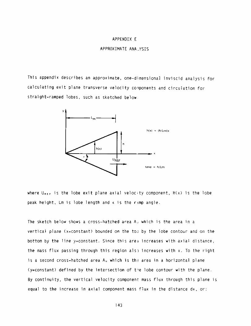
APPENDIX E

APPROXIMATE ANAL_YSIS

This appendix describes an approximate, one-d:imensiona] inviscid analysis for

calculating exit plane transverse velocity co;nponents and circulation for

straight-ramped lobes, such as sketched below

h

h(x} = (h/Lm)x

X

tane = hlLm

where URE_ is the lobe exit plane axial velocity component, H(x) is the lobe

peak height, Lm is lobe length and E is the ramp angle.

The sketch below shows a cross-hatched area A, which is the area in a

vertical plane (x=constant) bounded on the to_)by the lobe contour and on the

bottom by the line y=constant. Since this are:_ increases with axial distance,

the mass flux passing through this region als) increases with x. To the right

is a second cross-hatched area A, which is th,_)area in a horizontal plane

(y=constant) defined by the intersection of t!_e lobe contour with the plane.

By continuity, the vertical velocity component mass flux through this plane is

equal to the increase in axial component mass flux in the distance dx, or:

143

dA dAH V

V .... U REFdx dx

(E.I)

A V

z =0

w

z = L/2

IIIIIIVIIIItI

z II I

I-,_--- I×--_ I

' ' vl I

/ IIII

DASHED LINE GIVES

INTEGRATION CIRCUIT

L\ \",&

I(x) ÷ dl

constant density conditions. Since UREF iS known and the areas are functions

of lobe waveform, y and x, the vertical velocity component can be determined

as a function of X and y and lobe shape.

In the Following, the exit plane velocity was calculated as well as the

contribution of this component to circulation, F As sketched above, the

circulation path includes both vertical and horizontal legs. The present

analysis cannot treat the horizontal leg contribution, however, the section

titled "Circulation Calculations" in the main text shows this contribution is

negligibly small for large amplitude mixer lobes. Calculations are performed

for rectangular lobes, parallel sided lobes with peak regiond rounds,

triangular lobes and sinusoidal lobes.

144

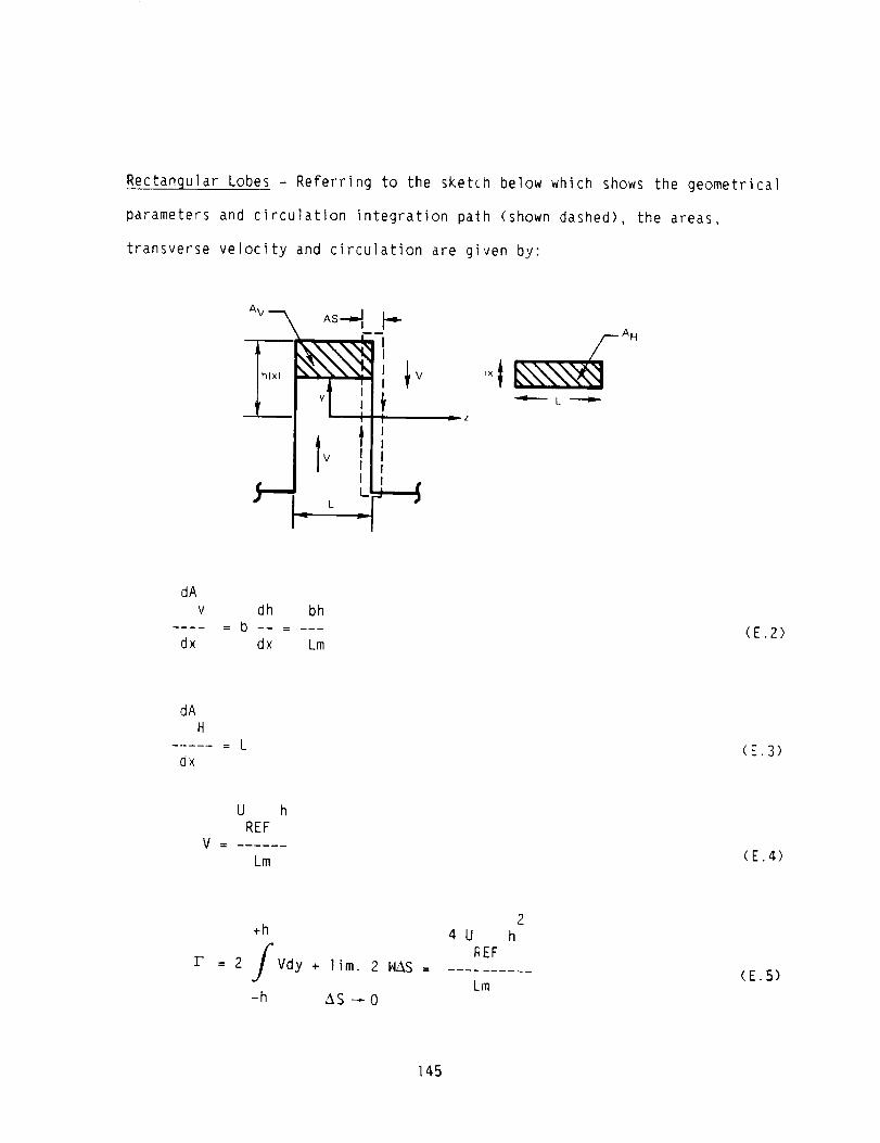
Rectanqular Lobes - Referring to the sketch below which shows the geometrical

parameters and circulation integration path (shown dashed), the areas,

transverse velocity and circulation are given by:

AV_ AS--_ _-

Itvfl,_ z

dx

dAV

dx

dh bh

dx Lm(E.2)

dAH

...... = Ldx

(E.3)

V

U h

REF

Lm(E.4)

÷h

= 2 J Vdy + lim. 2 N&S =£

-h _S _ 0

2

4U hREF

Lm(E.5)

145

Since the spanwise component, N, is finite, the horizontal leg contribution

for this lobe is zero. Vertical component magnitude within the lobe is

constant and directly dependent on the amplitude-to-length ratio (tangent of

the ramp angle• ). Circulation is dependent on the second power of lobe

amplitude.

Sinusoidal Lobes - Similar quantities for a sinusoidal lobe geometry are given

below:

A_h(x)_ S y = h(x) COS ('n'z/L)

lh Z

/,vLk I

dAv 2L dh

dx _ dx

2 2h-y

(E.6)

dA -I

H : 2L COS

dx

(y/h)

V

_/ 2U l-(ylh)

REFh

-I

L cos (y/h)

(E.7)

(E.8)

2I-' = 2.46U h

REF

146

(E.9)

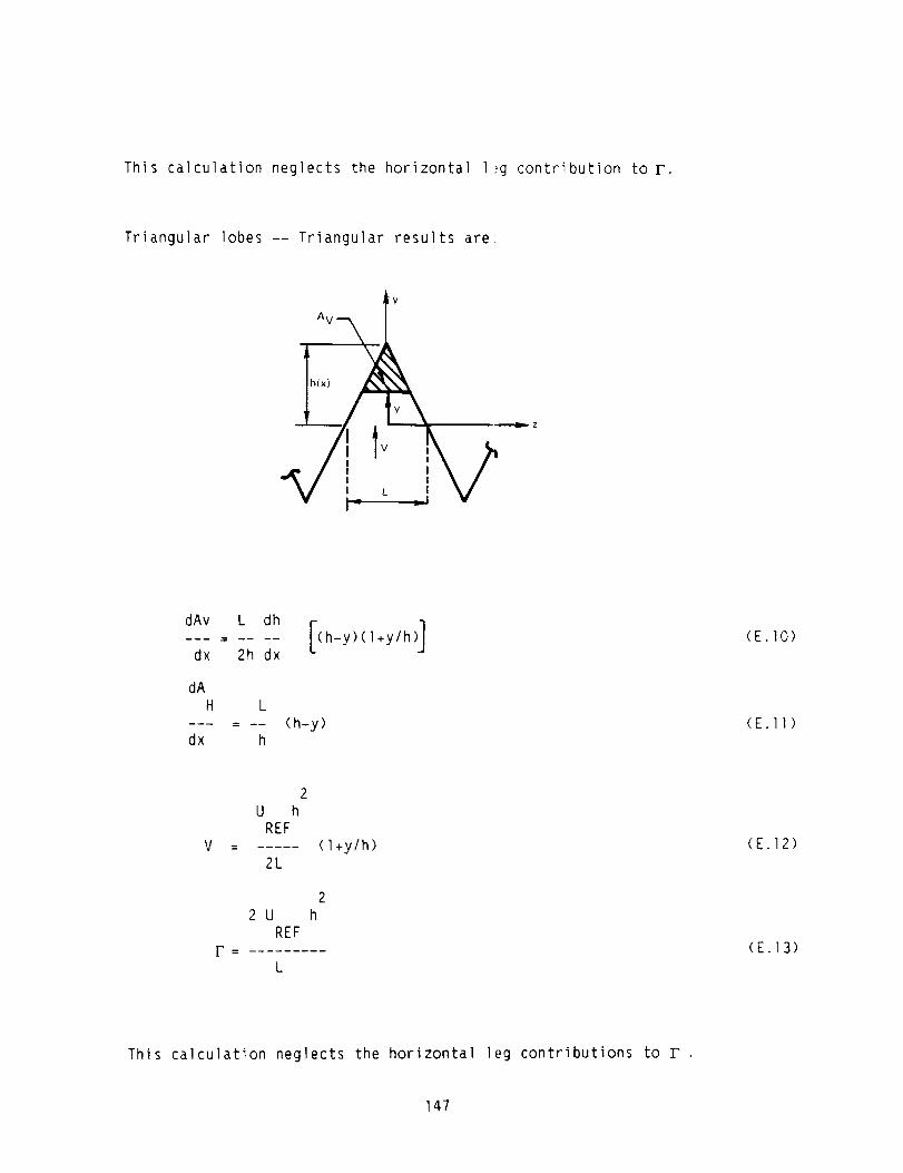
This calculation neglects the horizontal l_g contribution to F.

Triangular lobes -- Triangular results are-

I-

-_ Z

dAv

dx

dAH

dx

L dh

2h dx

L

h

(h-y)(l+y/h)]

(h-y)

(E.IO)

(E.11)

2U h

REF

2L(l+ylh)

22U h

REFP=

L

(E.12)

(E.13)

This calculation neglects the horizontal leg contributions to r .

147

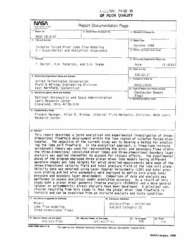
OF. P_OR QUALITY

Nat4o_al Aeronau!,cs andS_ace Adm,_,st,at,on

1 Report No,

NASA CR-41474 Title and Subtitle

Report Documentation Page

2 Government Accession No.

Turbofan Forced Mixer Lobe Flow ModelingI -Experimenta] and Analytical Assessment

7, Author(s)

T. Barber, R.N. Paterson, and S.A. Skebe

g Performing Organization Name and Address

United Technologies CorporationPratt & Nhitney Engineering DivisionEast Hartford, Connecticut

12. Sponsoring A_ncy Name and Address

Nationa] Aeronautics and Space AdministrationLewis Research CenterCleveland, Ohio 44135-3191

3 Reclpient's Calalog No

5. Report Date

October 1988

6, Performing Organization Code

8. Performing Organization Repo_ No.

None (E-4083)10. Work Unit No.

505-62-2111. Contract or Grant No,

NAS3-2303913. Type of Report and Peri_ Covered

Contractor ReportFinal

14. S_nsoring Agency Code

15. Supplementa_ Notes

Project Manager, Allan R.Research Center.

Bishop, Internal Fluid Mechanics Division, NASA Lewis

16. Abstract

This report describes a Joint analytical and experimental investigation of three-dlmensional flowfteld development within the lobe region of turbofan forced mlxernozzles. The objective of the current study was to develop a method for predict-ing the lobe exlt flowfteld. In the analytlcal approach, a llnearlzed lnviscidaerodynamlc theory was used for representing the axial and secondary flows withinthe three-dlmenslonal convo]uted mixer lobes and three-dlmenslonal boundary layeranalysis was applled thereafter to account for viscous effects. The experlmentalphase of the program employed three planar mixer lobe models having differentwaveform shapes and lobe heights for which detailed measurements were made of the

three-dlmenslonal velocity fleld and total pressure field at the lobe exlt plane.Velocity data was obtained using Laser Dopp]er Veloclmetry (LDV) and total pres-sure probing and hot wlre anemometry were employed to define exit plane totalpressure and boundary layer development. Comparison of data and analysis wasperformed to assess analytical model prediction accuracy. As a result of this

study both a planar mixer geometry inverse analysis (PLANMIX) and a more general(planar or axlsymmetrlc) dlrect analysls have been developed. A prlncipal con-cluslon resultlng from thls study is that the global mixer lobe flowfleld isinviscld and can be predicted from an Invlscld analysls and Kutta condition.

17. Key Words (Suggest_ by Aurar(s)) 118. Distribution Statement

Mixers I Unclassified - Unlimited

Lobe flow modeling Subject Category 02Three-dimensional flows

19. Security Clessif (of this re_R) I 20. Securi_ Classif. (of this page) 21, No of pages 22 Price*

Uncl_ssified l Unclassified 156 _

N_A FORM1626_T _ *For sate by the National T_hnical Information Service, Springfield, Virginia 22161

NASA-Langley, 1988

SPECIAL FOURTH-CLASS RATE

POSTAGE & FEES PAIDNASA

Permit No G-27

POSTMASTER: if Undeliverable (Section 158Postsl Manual) Do Not Return

4