Turbocharger 000
34
MEEN-646 T URBOMACHINERY F L OW P HYSICS P ROJECT 3 Design of an Integrated Turbocharger Author: Yuval DORON Presented to: Dr. T. S CHOBEIRI 4/26/2009
-
Upload
pinakin-panchal -
Category
Documents
-
view
249 -
download
1
Transcript of Turbocharger 000

8/3/2019 Turbocharger 000
http://slidepdf.com/reader/full/turbocharger-000 1/34
MEEN-646 TURBOMACHINERY FLOW PHYSICS
PROJECT 3
Design of an Integrated Turbocharger
Author:
Yuval DORON
Presented to:
Dr. T. SCHOBEIRI
4/26/2009
8/3/2019 Turbocharger 000
http://slidepdf.com/reader/full/turbocharger-000 2/34
Contents
1 Project Description 1
1.1 Introduction . . . . . . . . . . . . . . . . . . . . . . . . . . . . . . . . . . . . . . 1
1.2 Background . . . . . . . . . . . . . . . . . . . . . . . . . . . . . . . . . . . . . . 11.3 Objectives . . . . . . . . . . . . . . . . . . . . . . . . . . . . . . . . . . . . . . . 3
2 Project Tasks 4
2.1 Compressor Aero-thermodynamics . . . . . . . . . . . . . . . . . . . . . . . . . . 5
2.1.1 Compressor Solution . . . . . . . . . . . . . . . . . . . . . . . . . . . . . 6
2.2 Turbine Aero-thermodynamics . . . . . . . . . . . . . . . . . . . . . . . . . . . . 8
2.3 Compressor CAD Design . . . . . . . . . . . . . . . . . . . . . . . . . . . . . . . 9
2.3.1 Compressor Diffuser . . . . . . . . . . . . . . . . . . . . . . . . . . . . . 122.4 Turbine CAD Design . . . . . . . . . . . . . . . . . . . . . . . . . . . . . . . . . 13
2.4.1 Stator Blades . . . . . . . . . . . . . . . . . . . . . . . . . . . . . . . . . 16
3 Results 17
3.1 Complete Turbocharger Design . . . . . . . . . . . . . . . . . . . . . . . . . . . . 18
3.1.1 Bearing Calculations . . . . . . . . . . . . . . . . . . . . . . . . . . . . . 20
3.2 Conclusions . . . . . . . . . . . . . . . . . . . . . . . . . . . . . . . . . . . . . . 21
Appendices 22
i
8/3/2019 Turbocharger 000
http://slidepdf.com/reader/full/turbocharger-000 3/34
List of Figures
1.1 Figure shows from the left, Pratt & Whitney centrifugal compressor gas turbine.
Right, Siemens 35 MW axial compressor gas turbine . . . . . . . . . . . . . . . . 1
1.2 Figure shows two distinct turbochargers for different applications . . . . . . . . . . 3
2.1 Centrifugal compressor designed with Solidworks . . . . . . . . . . . . . . . . . . 9
2.2 Shown impeller with internal threads . . . . . . . . . . . . . . . . . . . . . . . . . 10
2.3 Shown impeller shaft & cap configuration . . . . . . . . . . . . . . . . . . . . . . 10
2.4 Impeller safety factor of 0.5 from stress analysis . . . . . . . . . . . . . . . . . . . 11
2.5 Impeller deformation results from stress analysis . . . . . . . . . . . . . . . . . . 11
2.6 Impeller safety factor of 2.1 from stress analysis . . . . . . . . . . . . . . . . . . . 12
2.7 Impeller deformation results from stress analysis . . . . . . . . . . . . . . . . . . 12
2.8 A cut section of the diffuser is shown, α3 = 15 . . . . . . . . . . . . . . . . . . . 132.9 Turbine and stator blade designed with Solidworks . . . . . . . . . . . . . . . . . 13
2.10 Turbine rotor designed with Solidworks . . . . . . . . . . . . . . . . . . . . . . . 14
2.11 Section cut shows added radius to internal hub diameter . . . . . . . . . . . . . . . 14
2.12 Final stress analysis shows rotor hub deformation . . . . . . . . . . . . . . . . . . 15
2.13 Final stress analysis shows rotor hub safety factor . . . . . . . . . . . . . . . . . . 15
2.14 iso surface clipping examination shows safety factor of .55 at blade tip close to hub 16
2.15 Stator blade designed on Solidworks . . . . . . . . . . . . . . . . . . . . . . . . . 16
3.1 Velocity triangle for the compressor stage . . . . . . . . . . . . . . . . . . . . . . 18
3.2 Velocity triangle for the turbine stage . . . . . . . . . . . . . . . . . . . . . . . . . 18
3.3 Complete turbocharger designed on Solidworks, cut view . . . . . . . . . . . . . . 19
3.4 Complete turbocharger designed on Solidworks, exploded view . . . . . . . . . . . 20
.5 Appendix A, Parametric Table solutions for the compressor from EES . . . . . . . 22
.6 Appendix B, Alloy steel used as a material choice for the compressor . . . . . . . 22
.7 Appendix C, Compressor calculations from EES . . . . . . . . . . . . . . . . . . . 23
.8 Appendix C, Compressor calculations from EES . . . . . . . . . . . . . . . . . . . 25
.9 Appendix C, Compressor calculations from EES . . . . . . . . . . . . . . . . . . . 26
.10 Appendix C, Turbine calculations from EES . . . . . . . . . . . . . . . . . . . . . 27
.11 Appendix C, Turbine calculations from EES . . . . . . . . . . . . . . . . . . . . . 28
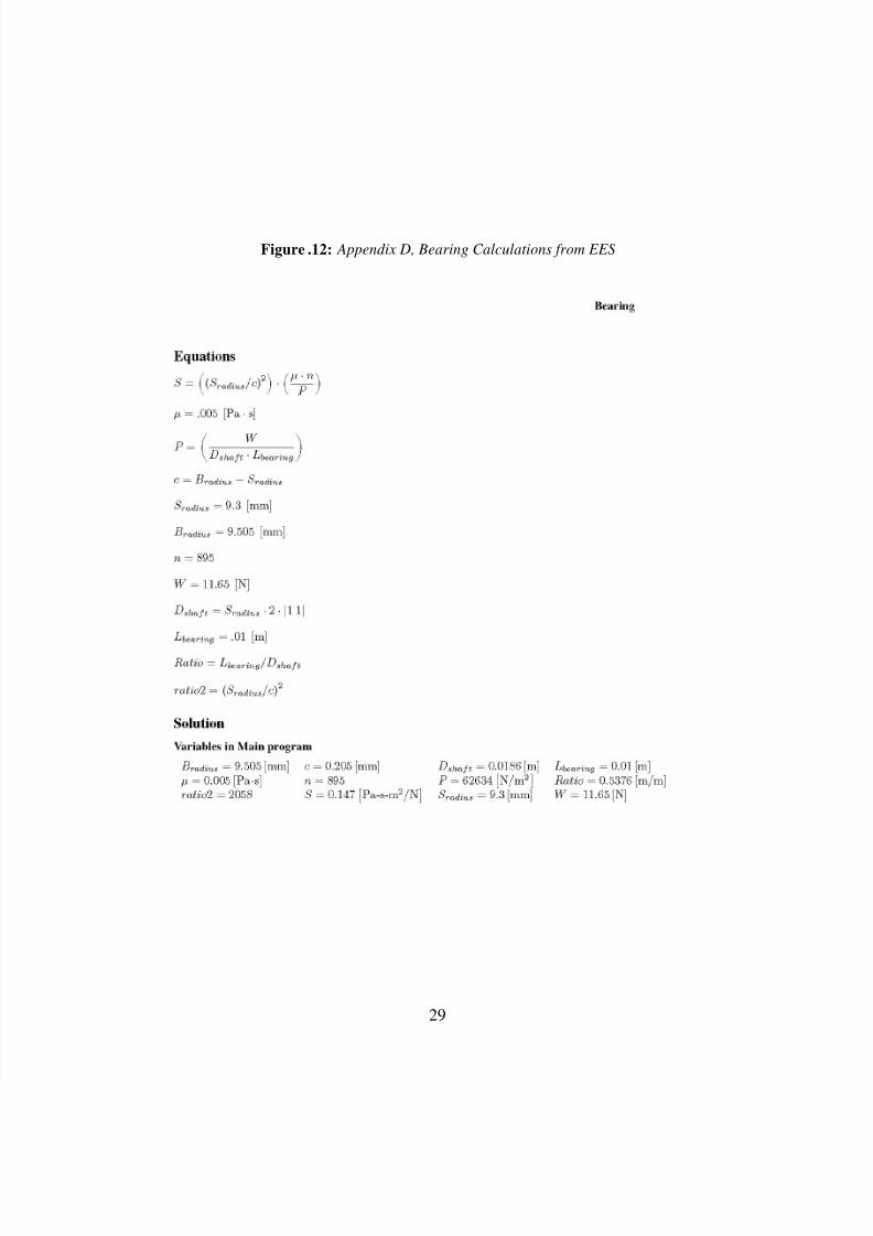
.12 Appendix D, Bearing Calculations from EES . . . . . . . . . . . . . . . . . . . . 29
ii

8/3/2019 Turbocharger 000
http://slidepdf.com/reader/full/turbocharger-000 4/34
List of Tables
2.1 Parameter list for compressor and turbine . . . . . . . . . . . . . . . . . . . . . . 5
3.1 Solved parameters for compressor and turbine . . . . . . . . . . . . . . . . . . . . 17
3.2 Table shows turbocharger components associated with either compressor or turbine 18
iii

8/3/2019 Turbocharger 000
http://slidepdf.com/reader/full/turbocharger-000 5/34
Abstract
A turbocharger is a device that adds air to the engine in order to increase power and ef-
ficiency. There are a great many variety of turbocharger designs which are dependent on
applications and manufacturing methodology. This project reports the complete solutions and
design for a turbocharger with some known data. Some of the Data provided was altered as
a necessity in order to find a viable solution. A complete aero thermodynamic analysis was
performed on the turbocharger turbine and compressor components, followed by a complete
design on a 3-D modeling software, in this case Solidworks. Stress analysis was performed
on different components to validate the design and overall performance. Results for the aero
thermodynamic properties are reported in a table format which includes all stage parameters
for both compressor and turbine. The project concludes with a calculation for the correct size
and geometry for the turbocharger bearings.
iv
8/3/2019 Turbocharger 000
http://slidepdf.com/reader/full/turbocharger-000 6/34
1 Project Description
1.1 Introduction
This project is the culmination of the complete fundamental study of turbomachinery flow physics.
Up to this juncture turbomachinery had been studied in component form,that is, compressors andturbines where explored in details but separately. Though both the compressor and turbine follow
identical analysis individually, combining the two into one machine and then solving for their op-
erating parameters is an involved process that may have more than one solution. In turbomachinery
there are only two types of machines that integrate both compressor and turbine into one machine:
• Turbocharger
• Gas Turbine Engine
A gas turbine engine differs from a turbocharger first by application and second by the working
principle. The gas turbine is designed in such a way that the compressor compresses the air thatis then combusted and is directed onto the turbine. The turbine is designed to generate enough
power to run the compressor in addition to generating net work. The turbine in the turbocharger
however, is not designed to generate any net work. Moreover, in the turbocharger the compressed
air from the compressor is utilized to enhance the performance of an internal combustion engine.
In addition, gas turbine engines are designed to operate with either a centrifugal compressor or
axial compressor, where as the turbocharger is designed exclusively with a centrifugal compressor.
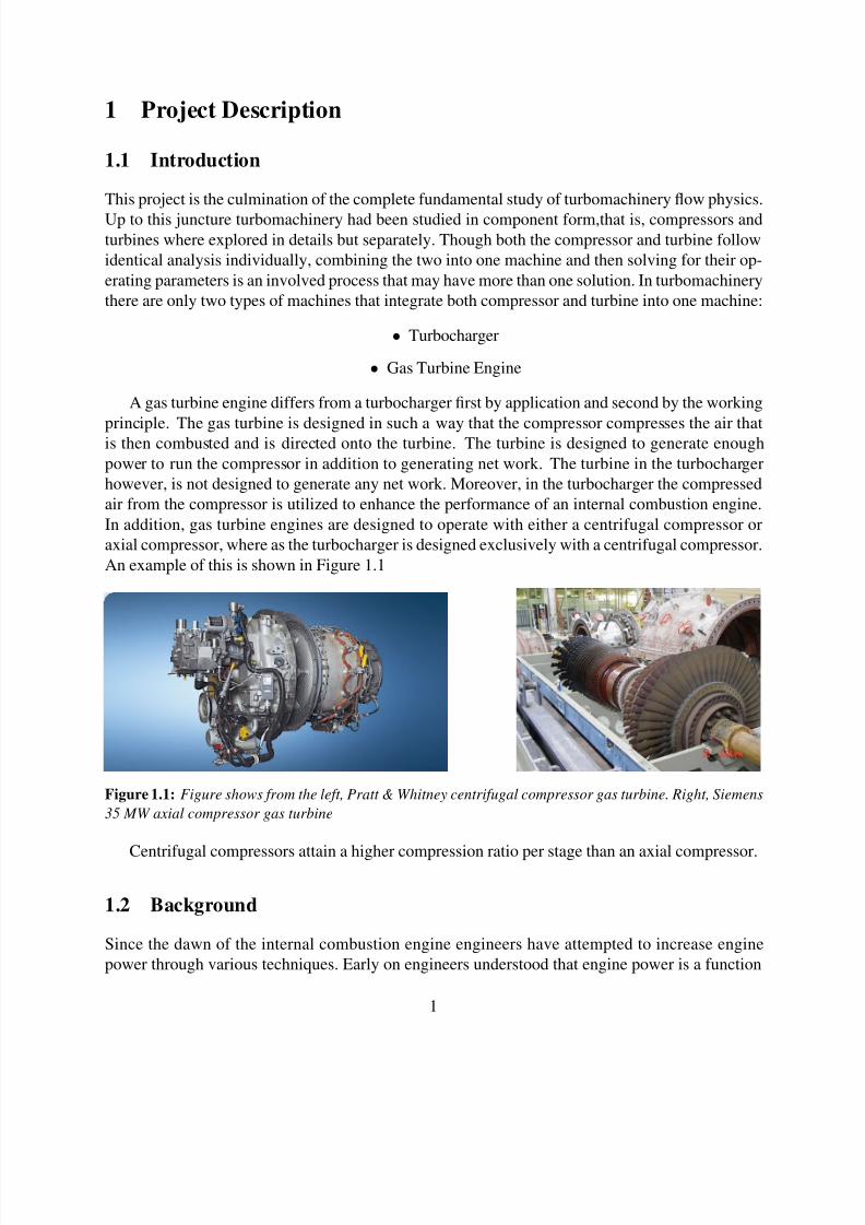
An example of this is shown in Figure 1.1
Figure 1.1: Figure shows from the left, Pratt & Whitney centrifugal compressor gas turbine. Right, Siemens
35 MW axial compressor gas turbine
Centrifugal compressors attain a higher compression ratio per stage than an axial compressor.
1.2 Background
Since the dawn of the internal combustion engine engineers have attempted to increase engine
power through various techniques. Early on engineers understood that engine power is a function
1

8/3/2019 Turbocharger 000
http://slidepdf.com/reader/full/turbocharger-000 7/34
of compression ratio, fuel grade, and the amount of air that enters piston chamber. In fact, it was
discovered that the amount of fuel that may be added per engine stroke is directly proportional
to the amount of air that enters the combustion chamber. This fact is due to the stoichiometric
balance that must be satisfied per combustion. The stoichiometric balance is satisfied when there
are enough oxygen molecules to completely react with all the fuel molecules. In fact, the definition
of a stoichiometric reaction is one where the exact amount of oxygen molecules react with the fuelinsuring no unburned fuel remains. However, since it is difficult to ensure a stoichiometric reaction,
it is common to allow more air per given reaction. The results of having too much oxygen or too
little oxygen per combustion produces what is known as a rich or a lean burn respectively. Though,
with the introduction of computerized fuel injection and ignition, engineers have closed the gap
between a stoichiometric reaction and a rich or lean reaction. A simple example of a stoichiometric
reaction using a combination fuel of Methane and Propane reacting with air is as follows:
.5CH 4 + .5C 3H 8 + 3.5 × (O2 + 3.76N 2) ⇒ 2CO2 + 3H 2O + 13.16N 2 (1.1)
Using the coefficients of the molecules in equation 1.1 it is possible to calculate the air to fuel
ratio, this ratio indicates the molecular weight of air to the molecular weight of fuel, and is asfollows:
AF s =(3.5 × (16× 2)) + (13.16 × (14× 2))
.5 × (12 + 4) + .5 × ((12× 3) + 8)(1.2)
The subscript s indicates a stoichiometric reaction. The AF S for this reaction as shown in equation
1.2 is 16.02, indicates that for every molecule of fuel there are 16.02 molecules of air. This simple
example shows that the amount fuel injected into the combustion cylinder is dependent on the
amount air that is mixed with the fuel. Therefor, it is evident that if the amount of air can be
increased per combustion cycle then more fuel can be introduced which generates more power per
combustion cycle.
The question then is how to add more air per stroke of a piston. To understand this it is firstcrucial to understand what parameter controls the amount of air that enters the piston chamber in
the first place. The simple answer is that, the amount of air is controlled by the piston draw itself.
The mechanism for drawing in air is controlled by vacuum that is created when the piston is in the
drawing cycle also known as the down stroke in a four stroke engine. As the piston moves down,
the intake valve is simultaneously opened to allow the air and fuel mixture to enter the cylinder
chamber. This means that which ever device is utilized for providing more air to the engine, it
must do so in the same period of time that it takes for the cylinder to traverse from the top position
to the bottom position.
There are a two such devices that enable more air to enter the cylinder per stroke, but in essence
they operate on the same principle. The two devices are:
1. Supercharger
2. Turbocharger
2
8/3/2019 Turbocharger 000
http://slidepdf.com/reader/full/turbocharger-000 8/34
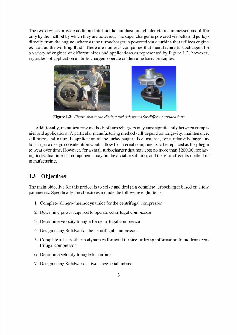
The two devices provide additional air into the combustion cylinder via a compressor, and differ
only by the method by which they are powered. The super charger is powered via belts and pulleys
directly from the engine, where as the turbocharger is powered via a turbine that utilizes engine
exhaust as the working fluid. There are numerus companies that manufacture turbochargers for
a variety of engines of different sizes and applications as represented by Figure 1.2, however,
regardless of application all turbochargers operate on the same basic principles.
Figure 1.2: Figure shows two distinct turbochargers for different applications
Additionally, manufacturing methods of turbochargers may vary significantly between compa-
nies and applications. A particular manufacturing method will depend on longevity, maintenance,
sell price, and naturally application of the turbocharger. For instance, for a relatively large tur-
bocharger a design consideration would allow for internal components to be replaced as they begin
to wear over time. However, for a small turbocharger that may cost no more than $200.00, replac-
ing individual internal components may not be a viable solution, and therefor affect its method of
manufacturing.
1.3 Objectives
The main objective for this project is to solve and design a complete turbocharger based on a few
parameters. Specifically the objectives include the following eight items:
1. Complete all aero-thermodynamics for the centrifugal compressor
2. Determine power required to operate centrifugal compressor
3. Determine velocity triangle for centrifugal compressor
4. Design using Solidworks the centrifugal compressor
5. Complete all aero-thermodynamics for axial turbine utilizing information found from cen-
trifugal compressor
6. Determine velocity triangle for turbine
7. Design using Solidworks a two stage axial turbine
3

8/3/2019 Turbocharger 000
http://slidepdf.com/reader/full/turbocharger-000 9/34
8. Design using Solidworks a complete turbocharger to include casing, bearings, labyrinth
seals, rotor, and volutes
The item list above represents not only the objectives sought in this project but also the process
path that was required to solve all the parameters for the turbocharger. What the list does not
describe however, is the exact methodology that is required to solve all equations. In fact as it wasdiscovered some of the parameters that were given in the problem for the turbocharger had to be
altered in order to converge on a solution. In particular, on the compressor side of the turbocharger,
either lowering the angular velocity ω, or reducing the impeller’s outer diameter was mandatory in
order to attain a converging solution. The exact path to the complete solution will be discussed in
detail in the following three sections.
2 Project Tasks
The complete analysis and design of a turbocharger is presented in this report. The turbochargeranalysis was performed utilizing Engineering Equation Solver, also known as EES, which permits
the user to enter all equations that are necessary to converge on a solution. However, if the solver
does not converge on a solution then a parametric table can be generated which permits the user to
alter values which are then used to converge on a solution. The latter was used in the compressor
analysis, see appendix A. The analysis for the turbocharger is constrained by the following two
main items:
• Compressor impeller and turbine should have similar out side diameters
• Turbine and impeller rotate at same rotational velocity
The reason for maintaining similar overall diameters for the turbine and compressor impeller is
based on ease of manufacturability and placement in the engine compartment. Having two very
different diameters would prove cumbersome when arranging other components that go in the en-
gine compartment. This is an example of a design consideration that is dependent on application.
The second constraint is due tot the fact that the impeller and turbine sit on the same shaft. This
constraint is found in most turbogenerators. In fact, various gas turbines are manufactured in a sim-
ilar fashion, however, some gas turbines operate with different rotational speeds for the compressor
and turbine. These types of gas turbines are manufactured with what is known as a spooling shaft.
This means that the turbine and compressor sit on different shafts that are one inside the other.
Other than these two main constraints a list of operational parameters were given in the problem
statement, however, some of these parameters had to be altered in order to converge on a solution.The initial parameters are given in table 2.1.
With these initial parameters it was possible to start the analysis employing the correct equa-
tions in EES. However, as it was discovered a solution could not be attained utilizing these initial
parameters. There for a parametric table was created in EES that permitted altering various param-
eters until a solution could be found. This method of converging on to a viable solution required
4
8/3/2019 Turbocharger 000
http://slidepdf.com/reader/full/turbocharger-000 10/34
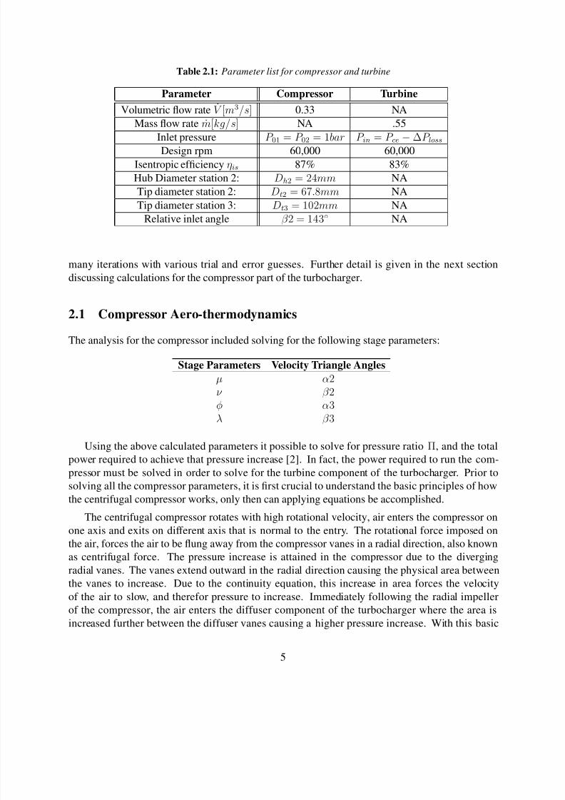
Table 2.1: Parameter list for compressor and turbine
Parameter Compressor Turbine
Volumetric flow rate V [m3/s] 0.33 NA
Mass flow rate m[kg/s] NA .55
Inlet pressure P 01 = P 02 = 1bar P in = P ce −∆P lossDesign rpm 60,000 60,000
Isentropic efficiency ηis 87% 83%
Hub Diameter station 2: Dh2 = 24mm NA
Tip diameter station 2: Dt2 = 67.8mm NA
Tip diameter station 3: Dt3 = 102mm NA
Relative inlet angle β 2 = 143◦ NA
many iterations with various trial and error guesses. Further detail is given in the next section
discussing calculations for the compressor part of the turbocharger.
2.1 Compressor Aero-thermodynamics
The analysis for the compressor included solving for the following stage parameters:
Stage Parameters Velocity Triangle Angles
µ α2ν β 2φ α3
λ β 3
Using the above calculated parameters it possible to solve for pressure ratio Π, and the total
power required to achieve that pressure increase [2]. In fact, the power required to run the com-
pressor must be solved in order to solve for the turbine component of the turbocharger. Prior to
solving all the compressor parameters, it is first crucial to understand the basic principles of how
the centrifugal compressor works, only then can applying equations be accomplished.
The centrifugal compressor rotates with high rotational velocity, air enters the compressor on
one axis and exits on different axis that is normal to the entry. The rotational force imposed on
the air, forces the air to be flung away from the compressor vanes in a radial direction, also known
as centrifugal force. The pressure increase is attained in the compressor due to the divergingradial vanes. The vanes extend outward in the radial direction causing the physical area between
the vanes to increase. Due to the continuity equation, this increase in area forces the velocity
of the air to slow, and therefor pressure to increase. Immediately following the radial impeller
of the compressor, the air enters the diffuser component of the turbocharger where the area is
increased further between the diffuser vanes causing a higher pressure increase. With this basic
5
8/3/2019 Turbocharger 000
http://slidepdf.com/reader/full/turbocharger-000 11/34
understanding for the impeller’s physics, the proper equations can be applied and a solution found.
After finding a solution, however, it should be examined and verified that it is a logical solution,
and this can only be achieved once the physics of the impeller are understood.
2.1.1 Compressor Solution
The first step in the process for finding a viable compressor solution is to solve for the thermo-
dynamic properties of the impeller. Beginning with the inlet temperature and using build in ther-
modynamic properties in EES, enthalpy and density at the inlet are found. Next the geometry is
defined for the inlet and outlet area, (see equation 2.1) however, since no information is given for
the outlet area, a guess value must be used. Additionally, since the outlet area is a function of exit
blade height and exit tip diameter, then the blade at the exit was parameterized in the parametric
table. In particular, a blade height of 3mm, 4mm, 5mm, 7.5mm, 10mm, and 12.5mm were used.
A2 = π/4 ·
D2
t2 −D2
h2
(2.1)
Now that the areas are known and given the inlet density, the inlet and outlet axial velocity can bedetermined using continuity (see equations 2.2& 2.3).
mcc2 = V · ρincc (2.2)
V 2 =mcc2
ρincc ·A2
(2.3)
Next the rest of the velocity triangle components are found using basic trigonometry, these are β 2,
U2, U3, W3, V3. The exit relative angle β 3 is set at 90◦. The exit angle α3, is also parameterized
in the parametric table, and W3 is set equal to V m3 (see equations 2.4, thru 2.10).
U 2 = ω · radiuscl (2.4)
radiuscl =
(Dt2/2) − (Dh2/2)
2
+ (Dh2/2) (2.5)
U 3 = (Dh3/2) · ω (2.6)
W 2 = V 22
+ U 22
(2.7)
β 2 = arccos (V 2/W 2) + 90 (2.8)
V 3 =U 3
Cos(α3)(2.9)
6

8/3/2019 Turbocharger 000
http://slidepdf.com/reader/full/turbocharger-000 12/34
W 3 = V 3 · sin(α3) (2.10)
The next set of equation are set solve both the exit absolute velocity and the exit temperature at
stage three. However, since the exit density is not known calculating exit temperature and velocity
depend both on exit area, and impeller’s rotation. In order to solve this open ended problem a
parametric table was generated (see Appendix A) using all the input equations. Additionally, aMach number equation was added in stage three in order to set an upper boundary on the system.
The mach number equation (see equation 2.11) in its basic form uses the gas constant which when
divided by the molecular weight of the local gas provides a more accurate solution. The Mach
number equation also uses the local temperature, which in this case is at stage three ( T 3) and
is also unknown. In order to find T 3 the ideal gas equation is used (see equation 2.13) which
incorporates the pressure ratio (R p) across the compressor. Of course this T 3 is the isentropic
temperature, and so the given compressor efficiency is used to find the actual temperature at stage
three (see equation 2.14). Initially it was unknown which Mach number would solve the system of
equations, however, after numerous guesses a Mach number of .8 proved to be a viable solution.
M = V 3 k ·
R/28.97
· T 3cc
(2.11)
Using equation 2.12 the density at the exit is calculated from mass flow and the axial component
of exit velocity, which in this case is W3.
ρ3 =mcc3
W 3 ·A3
(2.12)
T 3cc,is = (T 2cc) · (R p)k−1
k (2.13)
T 3cc = T 3cc,is − T 2cc
ηis + T 2cc (2.14)
The next step is solving for the specific power required to run the compressor. Using equation
2.15 and assuming that all the compression is dully performed by the impeller, gives λ = 1. At
this stage there are insufficient equations to solve the system, therefore an additional equation for
specific power is added. Equation 2.16 provides the remaining variables required to solve the
system.
lm = λ · U 23
(2.15)
lm = c p · (T 3cc − T 2cc) +
.5 ·
V 23− V 2
2
(2.16)
All that remains now in order to converge on a reasonable solution is to run the parametric analysis
that is also created in EES. In this parametric table (see appendix A) as previously discussed, 6
different tables were generated, where the varying parameter between the tables was the exit bladeheight. However, for each particular table the varying parameter was the rotational speed of the
compressor. The last step in the analysis is to solve for all stage coefficients, the results for these
are shown in table 3.1. This concludes the analysis for the compressor, the cad design for the
compressor will be shown in section 2.3. The next section will discuss the solution for the turbine
component of the turbocharger.
7

8/3/2019 Turbocharger 000
http://slidepdf.com/reader/full/turbocharger-000 13/34
2.2 Turbine Aero-thermodynamics
The solution for the turbine component of the turbocharger was not as complex as the compressor
component and depended only the power found from the compressor problem. In fact, the solution
is straight forward and did not require any assumptions. Moreover, all essential parameters to find
a solution were given, assuming of course that a solution for the compressor power was found.Similar to the compressor problem, the main objective for the turbine component is to solve for
the total power that the turbine is expected to provide, in addition to all stage coefficients and all
angles in the velocity triangle (see table in section 2.1). The rotational velocity of the turbine as
previously mentioned is equal to the compressor’s since both compressor and turbine reside on the
same shaft. Similarly to the compressor analysis, the turbine analysis was performed using EES,
though no parametric table was required.
To begin the analysis the thermodynamic properties for the turbine were found using EES built
in functions. Next using the provided information in the problem statement the total power that
the turbine must provide was found using equations 2.17 thru 2.19. To clarify the Bloss in equation
2.18 refers to the power lost in the bearings of the turbine.
ηt = .83 (2.17)
Bloss = .1 · P wrt (2.18)
P wrt =31.51 + Bloss
ηt
(2.19)
The next section in the analysis is set to solve for all velocity triangle components including all
stage coefficients. However, this step required some predesign concepts to be chosen. In particular,
since this turbine is composed of both stator and rotating blades, a 50% degree of reaction was
established. Second, a 20 degree absolute angle was chosen for the inlet of the rotating blades.
With these two chosen parameters the complete analysis could be completed (see equations 2.20thru 2.29).
U 2 = ((Dh/2) + (Bh/2)) · ω (2.20)
V m2 =mt
ρin ·A(2.21)
V 2 =V m2
sin(α2)(2.22)
V u2 = V 2 · Cos(α2) (2.23)
lm =1000 · P wrt
mt
(2.24)
λ =lmU 23
(2.25)
V 3 = W 2 (2.26)
W 2 =
V 2m2
+ (V u2 − U 2)2 (2.27)
8
8/3/2019 Turbocharger 000
http://slidepdf.com/reader/full/turbocharger-000 14/34
β 2 = arcsin (V m2/W 2) (2.28)
V u3 = V 3 · Cos(β 2) (2.29)
The Complete set of equations for both the compressor and turbine will be shown in the appendix
C. However, the results for stage coefficients are shown in table 3.1 in section 3.
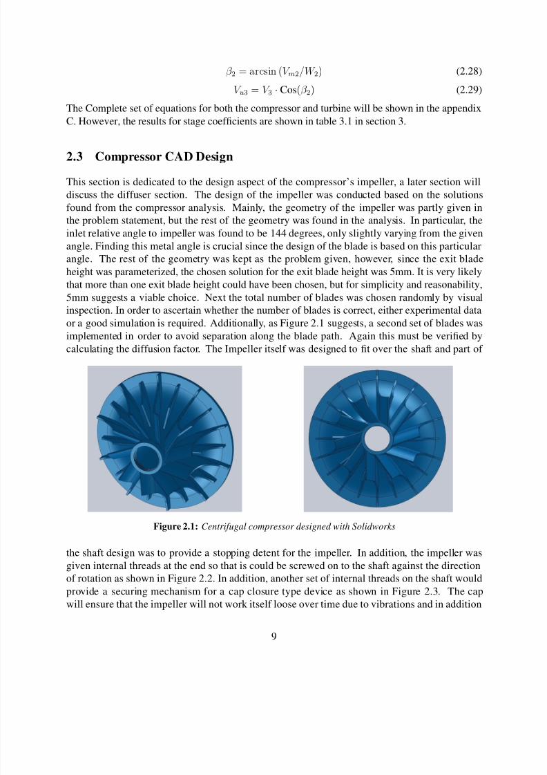
2.3 Compressor CAD Design
This section is dedicated to the design aspect of the compressor’s impeller, a later section will
discuss the diffuser section. The design of the impeller was conducted based on the solutions
found from the compressor analysis. Mainly, the geometry of the impeller was partly given in
the problem statement, but the rest of the geometry was found in the analysis. In particular, the
inlet relative angle to impeller was found to be 144 degrees, only slightly varying from the given
angle. Finding this metal angle is crucial since the design of the blade is based on this particular
angle. The rest of the geometry was kept as the problem given, however, since the exit blade
height was parameterized, the chosen solution for the exit blade height was 5mm. It is very likelythat more than one exit blade height could have been chosen, but for simplicity and reasonability,
5mm suggests a viable choice. Next the total number of blades was chosen randomly by visual
inspection. In order to ascertain whether the number of blades is correct, either experimental data
or a good simulation is required. Additionally, as Figure 2.1 suggests, a second set of blades was
implemented in order to avoid separation along the blade path. Again this must be verified by
calculating the diffusion factor. The Impeller itself was designed to fit over the shaft and part of
Figure 2.1: Centrifugal compressor designed with Solidworks
the shaft design was to provide a stopping detent for the impeller. In addition, the impeller was
given internal threads at the end so that is could be screwed on to the shaft against the direction
of rotation as shown in Figure 2.2. In addition, another set of internal threads on the shaft would
provide a securing mechanism for a cap closure type device as shown in Figure 2.3. The cap
will ensure that the impeller will not work itself loose over time due to vibrations and in addition
9

8/3/2019 Turbocharger 000
http://slidepdf.com/reader/full/turbocharger-000 15/34
Figure 2.2: Shown impeller with internal threads
Figure 2.3: Shown impeller shaft & cap configuration
will provide a smooth body for the incoming air. An additional consideration in the design is the
impeller’s material specification. The selected material is dependent on manufacturability, cost,
and stress analysis on the impeller. The stress analysis is performed on COSMOS a Solidworks
program that resides in the Solidworks interface. COSMOS is capable of performing various
stress analysis, one of which is applied centrifugal forces. This analysis was performed on both
the impeller and turbine rotor. For this part of the design, a stainless alloy was chosen as the basematerial, however, after a performed stress analysis using centrifugal loads, a safety factor of 0.5
was attained. A safety factor of 0.5 is insufficient, and therefor other materials were selected and
retested. A strong alloy was selected in the end after stress analysis results proved a safety factor
of 2. Figure 2.4 shows the safety factor results and Figure 2.5 shows deformation from the stress
analysis on stainless steel impeller.
10
8/3/2019 Turbocharger 000
http://slidepdf.com/reader/full/turbocharger-000 16/34
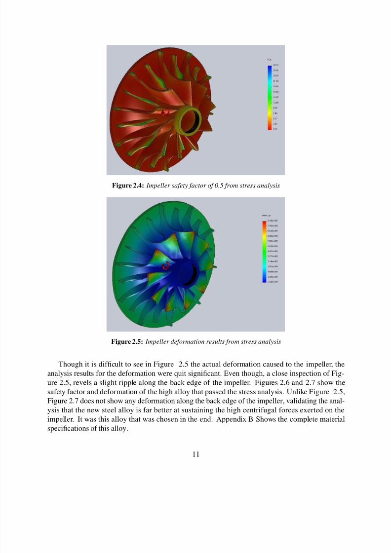
Figure 2.4: Impeller safety factor of 0.5 from stress analysis
Figure 2.5: Impeller deformation results from stress analysis
Though it is difficult to see in Figure 2.5 the actual deformation caused to the impeller, the
analysis results for the deformation were quit significant. Even though, a close inspection of Fig-
ure 2.5, revels a slight ripple along the back edge of the impeller. Figures 2.6 and 2.7 show the
safety factor and deformation of the high alloy that passed the stress analysis. Unlike Figure 2.5,
Figure 2.7 does not show any deformation along the back edge of the impeller, validating the anal-
ysis that the new steel alloy is far better at sustaining the high centrifugal forces exerted on the
impeller. It was this alloy that was chosen in the end. Appendix B Shows the complete material
specifications of this alloy.
11
8/3/2019 Turbocharger 000
http://slidepdf.com/reader/full/turbocharger-000 17/34
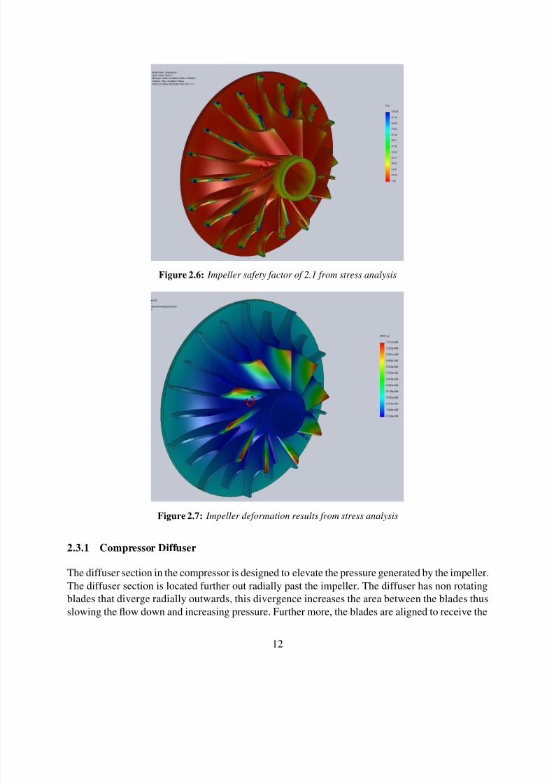
Figure 2.6: Impeller safety factor of 2.1 from stress analysis
Figure 2.7: Impeller deformation results from stress analysis
2.3.1 Compressor Diffuser
The diffuser section in the compressor is designed to elevate the pressure generated by the impeller.
The diffuser section is located further out radially past the impeller. The diffuser has non rotating
blades that diverge radially outwards, this divergence increases the area between the blades thus
slowing the flow down and increasing pressure. Further more, the blades are aligned to receive the
12
8/3/2019 Turbocharger 000
http://slidepdf.com/reader/full/turbocharger-000 18/34
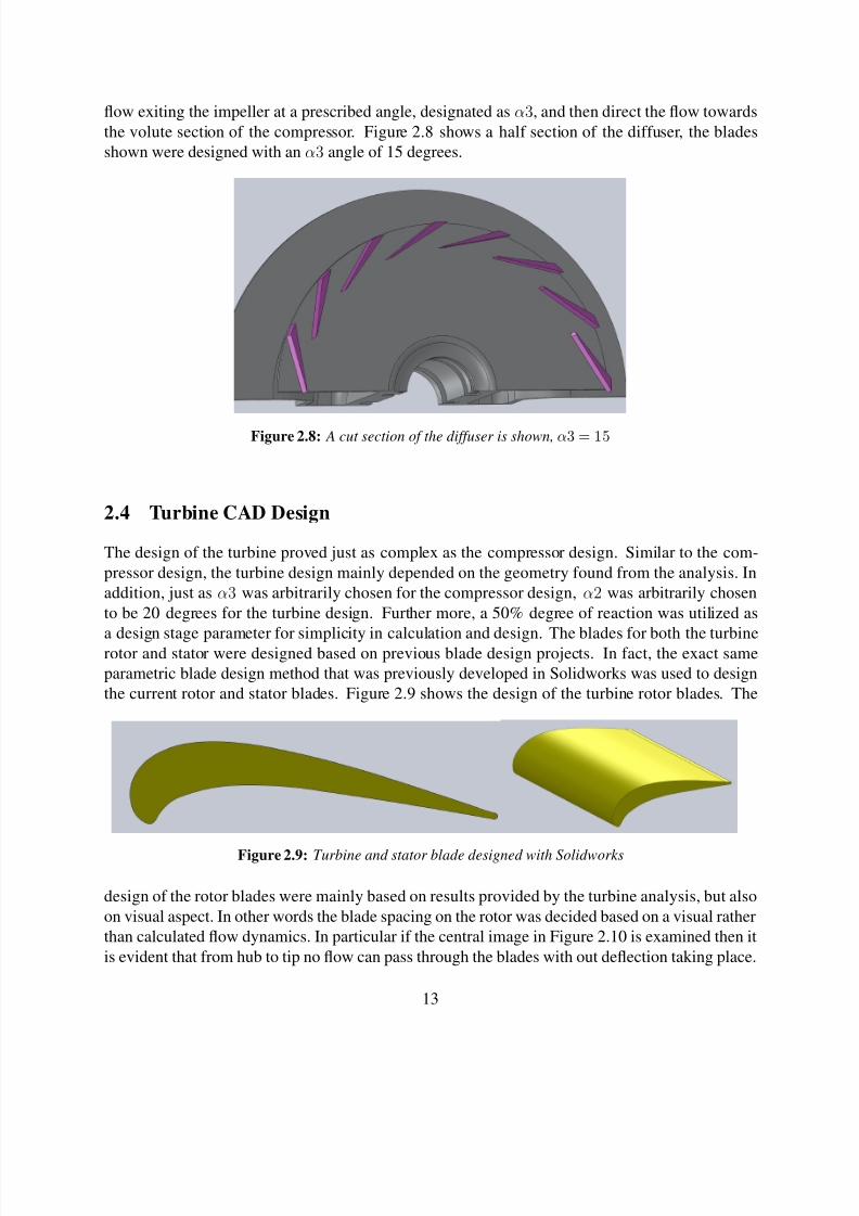
flow exiting the impeller at a prescribed angle, designated as α3, and then direct the flow towards
the volute section of the compressor. Figure 2.8 shows a half section of the diffuser, the blades
shown were designed with an α3 angle of 15 degrees.
Figure 2.8: A cut section of the diffuser is shown, α3 = 15
2.4 Turbine CAD Design
The design of the turbine proved just as complex as the compressor design. Similar to the com-
pressor design, the turbine design mainly depended on the geometry found from the analysis. In
addition, just as α3 was arbitrarily chosen for the compressor design, α2 was arbitrarily chosen
to be 20 degrees for the turbine design. Further more, a 50% degree of reaction was utilized as
a design stage parameter for simplicity in calculation and design. The blades for both the turbinerotor and stator were designed based on previous blade design projects. In fact, the exact same
parametric blade design method that was previously developed in Solidworks was used to design
the current rotor and stator blades. Figure 2.9 shows the design of the turbine rotor blades. The
Figure 2.9: Turbine and stator blade designed with Solidworks
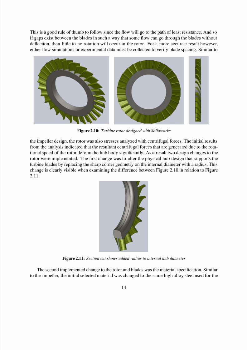
design of the rotor blades were mainly based on results provided by the turbine analysis, but also
on visual aspect. In other words the blade spacing on the rotor was decided based on a visual rather
than calculated flow dynamics. In particular if the central image in Figure 2.10 is examined then it
is evident that from hub to tip no flow can pass through the blades with out deflection taking place.
13
8/3/2019 Turbocharger 000
http://slidepdf.com/reader/full/turbocharger-000 19/34
This is a good rule of thumb to follow since the flow will go to the path of least resistance. And so
if gaps exist between the blades in such a way that some flow can go through the blades without
deflection, then little to no rotation will occur in the rotor. For a more accurate result however,
either flow simulations or experimental data must be collected to verify blade spacing. Similar to
Figure 2.10: Turbine rotor designed with Solidworks
the impeller design, the rotor was also stresses analyzed with centrifugal forces. The initial results
from the analysis indicated that the resultant centrifugal forces that are generated due to the rota-
tional speed of the rotor deform the hub body significantly. As a result two design changes to the
rotor were implemented. The first change was to alter the physical hub design that supports the
turbine blades by replacing the sharp corner geometry on the internal diameter with a radius. This
change is clearly visible when examining the difference between Figure 2.10 in relation to Figure
2.11.
Figure 2.11: Section cut shows added radius to internal hub diameter
The second implemented change to the rotor and blades was the material specification. Similar
to the impeller, the initial selected material was changed to the same high alloy steel used for the
14
8/3/2019 Turbocharger 000
http://slidepdf.com/reader/full/turbocharger-000 20/34
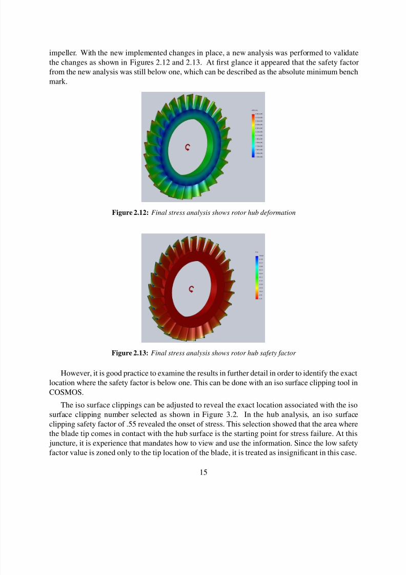
impeller. With the new implemented changes in place, a new analysis was performed to validate
the changes as shown in Figures 2.12 and 2.13. At first glance it appeared that the safety factor
from the new analysis was still below one, which can be described as the absolute minimum bench
mark.
Figure 2.12: Final stress analysis shows rotor hub deformation
Figure 2.13: Final stress analysis shows rotor hub safety factor
However, it is good practice to examine the results in further detail in order to identify the exact
location where the safety factor is below one. This can be done with an iso surface clipping tool in
COSMOS.
The iso surface clippings can be adjusted to reveal the exact location associated with the isosurface clipping number selected as shown in Figure 3.2. In the hub analysis, an iso surface
clipping safety factor of .55 revealed the onset of stress. This selection showed that the area where
the blade tip comes in contact with the hub surface is the starting point for stress failure. At this
juncture, it is experience that mandates how to view and use the information. Since the low safety
factor value is zoned only to the tip location of the blade, it is treated as insignificant in this case.
15

8/3/2019 Turbocharger 000
http://slidepdf.com/reader/full/turbocharger-000 21/34
Figure 2.14: iso surface clipping examination shows safety factor of .55 at blade tip close to hub
In other words, the low safety factor at that location does not affect the entire stability of the
construction, nor is there any deformation at that location. This indicates that there may be some
unresolved stresses at the tip, however, it is not enough to cause any failure to the rotor hub.
2.4.1 Stator Blades
The turbine in the turbogenerator is designed as a two stage turbine incorporating a row of station-
ary blades followed by a row of rotating blades. The analysis performed in EES calculated the total
power generated by the turbine using a 50% degree of reaction. However, unlike the rotating blade
which has a metal angle of 20 degrees (α2) at the inlet, the stator blades receive the flow head on at
90 degrees. The stator blade is designed to deflect the flow and align it with the metal angle of the
rotating blades. The velocity triangles will show the corresponding angles and magnitudes for the
turbine in the results section. The difference in design pertaining to the flow deflection between
Figure 2.15: Stator blade designed on Solidworks
the rotating and stator blades is evident when examining Figure 2.9 in comparison to Figure 2.15.
It is this profile difference between the blades that constitutes how the flow is deflected, and how
much power is generated in the turbine due to this deflection.
16
8/3/2019 Turbocharger 000
http://slidepdf.com/reader/full/turbocharger-000 22/34
3 Results
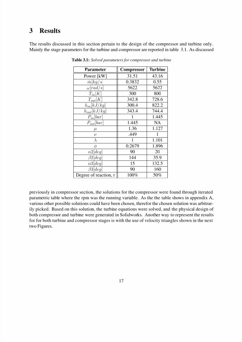
The results discussed in this section pertain to the design of the compressor and turbine only.
Mainly the stage parameters for the turbine and compressor are reported in table 3.1. As discussed
Table 3.1: Solved parameters for compressor and turbine
Parameter Compressor Turbine
Power [kW] 31.51 43.16
m[kg/s] 0.3832 0.55
ω[rad/s] 5622 5622
T in[K ] 300 800
T out[K ] 342.8 728.6
hin[kJ/kg] 300.4 822.2
hout[kJ/kg] 343.4 744.4
P in[bar] 1 1.445
P out[bar] 1.445 NA
µ 1.36 1.127
ν .449 1
λ 1 1.101
φ 0.2679 1.896
α2[deg] 90 20
β 2[deg] 144 35.9
α3[deg] 15 132.5
β 3[deg] 90 160
Degree of reaction, r 100% 50%
previously in compressor section, the solutions for the compressor were found through iterated
parametric table where the rpm was the running variable. As the the table shows in appendix A,
various other possible solutions could have been chosen, therefor the chosen solution was arbitrar-
ily picked. Based on this solution, the turbine equations were solved, and the physical design of
both compressor and turbine were generated in Solidworks. Another way to represent the results
for for both turbine and compressor stages is with the use of velocity triangles shown in the next
two Figures.
17
8/3/2019 Turbocharger 000
http://slidepdf.com/reader/full/turbocharger-000 23/34
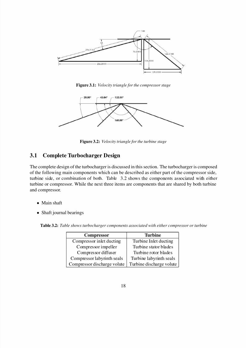
Figure 3.1: Velocity triangle for the compressor stage
Figure 3.2: Velocity triangle for the turbine stage
3.1 Complete Turbocharger Design
The complete design of the turbocharger is discussed in this section. The turbocharger is composed
of the following main components which can be described as either part of the compressor side,
turbine side, or combination of both. Table 3.2 shows the components associated with either
turbine or compressor. While the next three items are components that are shared by both turbineand compressor.
• Main shaft
• Shaft journal bearings
Table 3.2: Table shows turbocharger components associated with either compressor or turbine
Compressor Turbine
Compressor inlet ducting Turbine Inlet ducting
Compressor impeller Turbine stator blades
Compressor diffuser Turbine rotor blades
Compressor labyrinth seals Turbine labyrinth seals
Compressor discharge volute Turbine discharge volute
18

8/3/2019 Turbocharger 000
http://slidepdf.com/reader/full/turbocharger-000 24/34
• Turbine and Compressor casing
The geometry of both the turbine and compressor directly followed the results from the anal-
ysis, and therefor little guess work was needed in the design of both. However, designing the
casing for the turbocharger, including the inlet to the compressor, inlet to the turbine, both volutes,
labyrinth seals, and bearings, proved a great challenge. At the onset of the design there were manyoptions to follow, and many possible configurations for the turbocharger. Dimensions were arbi-
trarily chosen for the various components. The only source of information by which the design
should follow were pictures found on the internet. Naturally different manufacturers have their
own designs which are based on years of trial and error and experimentations. Therefor choosing
by which picture the base design should follow was difficult. At the end the design followed a com-
bination of pictures found on the internet, experience, and manufacturability for the end product.
Figure 3.3 shows a cut view of the completed assembled turbocharger.
Figure 3.3: Complete turbocharger designed on Solidworks, cut view
A paramount condition for the design was the feasibility of manufacturing. This means that the
design was not to be a simple block design, a mere suggestion of how the turbocharger should be
configured. Rather, a detailed design showing precisely how each component can be manufactured,
and then attached to the other components was the prescribed method used. An example would be
for the casing of the turbocharger. The casing could not be simply drawn as one component and
then assembled to cover the turbine and compressor. Rather, the casing has to be manufactured
from two sections that can accept the assembled turbine and compressor and inclose them properly.
Another example is the impeller which cannot be drawn with the shaft as one component, the
impeller is manufactured separately and is then assembled onto the shaft in a manner that ensures
19
8/3/2019 Turbocharger 000
http://slidepdf.com/reader/full/turbocharger-000 25/34
it from falling off during operation. This type of design methodology was incorporated for the
turbocharger design.
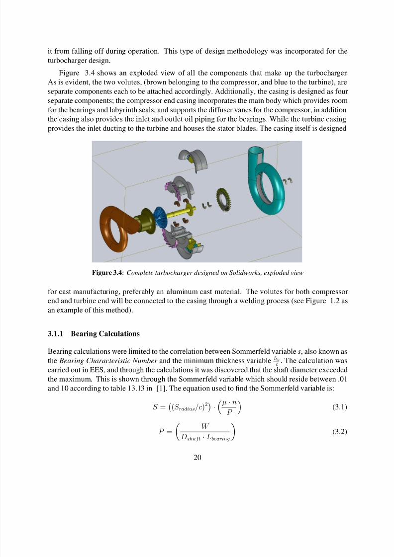
Figure 3.4 shows an exploded view of all the components that make up the turbocharger.
As is evident, the two volutes, (brown belonging to the compressor, and blue to the turbine), are
separate components each to be attached accordingly. Additionally, the casing is designed as four
separate components; the compressor end casing incorporates the main body which provides room
for the bearings and labyrinth seals, and supports the diffuser vanes for the compressor, in addition
the casing also provides the inlet and outlet oil piping for the bearings. While the turbine casing
provides the inlet ducting to the turbine and houses the stator blades. The casing itself is designed
Figure 3.4: Complete turbocharger designed on Solidworks, exploded view
for cast manufacturing, preferably an aluminum cast material. The volutes for both compressorend and turbine end will be connected to the casing through a welding process (see Figure 1.2 as
an example of this method).
3.1.1 Bearing Calculations
Bearing calculations were limited to the correlation between Sommerfeld variable s, also known as
the Bearing Characteristic Number and the minimum thickness variable hoc
. The calculation was
carried out in EES, and through the calculations it was discovered that the shaft diameter exceeded
the maximum. This is shown through the Sommerfeld variable which should reside between .01
and 10 according to table 13.13 in [1]. The equation used to find the Sommerfeld variable is:
S =
(S radius/c)2·
µ · n
P
(3.1)
P =
W
Dshaft · Lbearing
(3.2)
20
8/3/2019 Turbocharger 000
http://slidepdf.com/reader/full/turbocharger-000 26/34
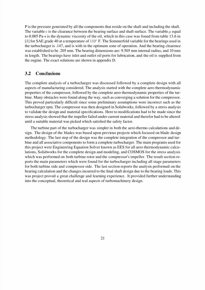
P is the pressure generated by all the components that reside on the shaft and including the shaft.
The variable c is the clearance between the bearing surface and shaft surface. The variable µ equal
to 0.005 Pa-s is the dynamic viscosity of the oil, which in this case was found from table 13.6 in
[1] for SAE grade 40 at a temperature of 110◦ F. The Sommerfeld variable for the bearings used in
the turbocharger is .147, and is with in the optimum zone of operation. And the bearing clearence
was established to be .205 mm. The bearing dimensions are: 9.505 mm internal radius, and 10 mmin length. The bearings have inlet and outlet oil ports for lubrication, and the oil is supplied from
the engine. The exact solutions are shown in appendix D.
3.2 Conclusions
The complete analysis of a turbocharger was discussed followed by a complete design with all
aspects of manufacturing considered. The analysis started with the complete aero thermodynamic
properties of the compressor, followed by the complete aero thermodynamic properties of the tur-
bine. Many obstacles were found along the way, such as converging a solution for the compressor.
This proved particularly difficult since some preliminary assumptions were incorrect such as theturbocharger rpm. The compressor was then designed in Solidworks, followed by a stress analysis
to validate the design and material specifications. Here to modifications had to be made since the
stress analysis showed that the impeller failed under current material and therefor had to be altered
until a suitable material was picked which satisfied the safety factor.
The turbine part of the turbocharger was simpler in both the aero-thermo calculations and de-
sign. The design of the blades was based upon previous projects which focused on blade design
methodology. The last step of the design was the complete integration of the compressor and tur-
bine and all associative components to form a complete turbocharger. The main programs used for
this project were Engineering Equation Solver known as EES for all aero thermodynamic calcu-
lations, Solidworks for the complete design and modeling, and COSMOS for the stress analysiswhich was performed on both turbine rotor and the compressor’s impeller. The result section re-
ports the main parameters which were found for the turbocharger including all stage parameters
for both turbine side and compressor side. The last section reports the analysis performed on the
bearing calculation and the changes incurred to the final shaft design due to the bearing loads. This
was project proved a great challenge and learning experience. It provided further understanding
into the conceptual, theoretical and real aspects of turbomachinery design.
21
8/3/2019 Turbocharger 000
http://slidepdf.com/reader/full/turbocharger-000 27/34
Appendices
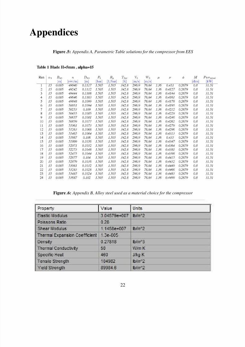
Figure .5: Appendix A, Parametric Table solutions for the compressor from EES
Figure .6: Appendix B, Alloy steel used as a material choice for the compressor
22
8/3/2019 Turbocharger 000
http://slidepdf.com/reader/full/turbocharger-000 28/34
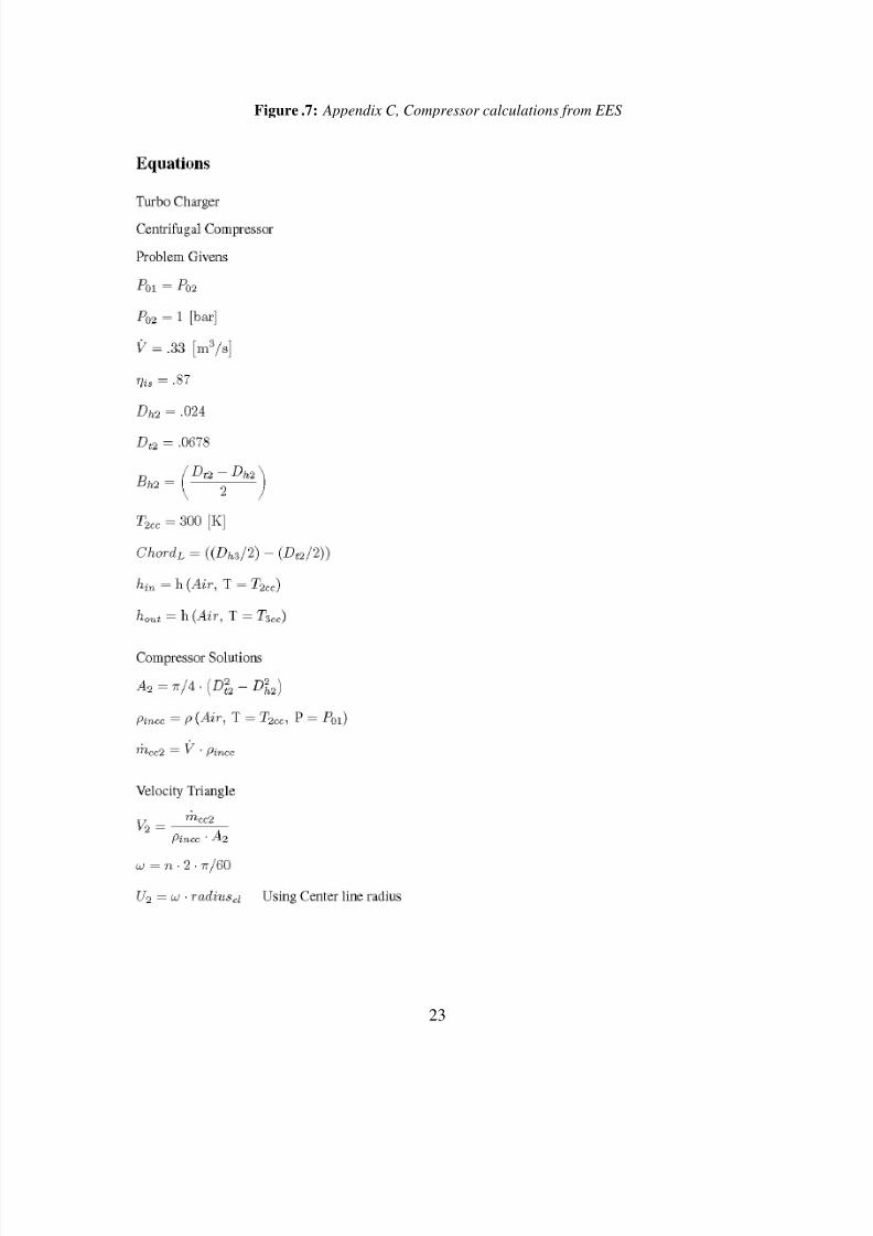
Figure .7: Appendix C, Compressor calculations from EES
23

8/3/2019 Turbocharger 000
http://slidepdf.com/reader/full/turbocharger-000 29/34
References
[1] Kurt M. Marshek Robert C. Juvinall. Fundamentals of Machine Component Design. John
Wiley &Sons,Inc, 3rd edition, 2000.
[2] Meinhard Schobeiri. Turbomachinery Flow Physics and Dynamic Performance. Springer,2005.
24
8/3/2019 Turbocharger 000
http://slidepdf.com/reader/full/turbocharger-000 30/34
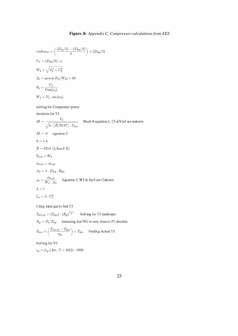
Figure .8: Appendix C, Compressor calculations from EES
25

8/3/2019 Turbocharger 000
http://slidepdf.com/reader/full/turbocharger-000 31/34
Figure .9: Appendix C, Compressor calculations from EES
26

8/3/2019 Turbocharger 000
http://slidepdf.com/reader/full/turbocharger-000 32/34
Figure .10: Appendix C, Turbine calculations from EES
27

8/3/2019 Turbocharger 000
http://slidepdf.com/reader/full/turbocharger-000 33/34
Figure .11: Appendix C, Turbine calculations from EES
28
8/3/2019 Turbocharger 000
http://slidepdf.com/reader/full/turbocharger-000 34/34
Figure .12: Appendix D, Bearing Calculations from EES