
Tunable Laser Optics
287
Transcript of Tunable Laser Optics


TUNABLE LASER OPTICS

This Page Intentionally Left Blank

TUNABLE LASER OPTICS
Francisco J. Duarte Eastman Kodak Company Research Laboratories Rochester, New York
ELSEVIER ACADEMIC
PRESS
Amsterdam Boston Heidelberg London New York Oxford Paris San Diego San Francisco Singapore Sydney Tokyo
This book is printed on acid-free paper. @
Copyright 2003, Elsevier Science (USA). All rights reserved.
No part of this publication may be reproduced or transmitted in any form or by any means, electronic or mechanical, including photocopy, recording, or any information storage and retrieval system, without permission in writing from the publisher.
Permissions may be sought directly from Elsevier's Science & Technology Rights Department in Oxford, UK: phone: (+44) 1865 843830, fax: (+44) 1865 853333, e-mail: [email protected]. You may also complete your request on-line via the Elsevier Science homepage (http://elsevier.com), by selecting "Customer Support" and then "Obtaining Permissions."
ACADEMIC PRESS An imprint of Elsevier Science 525 B Street, Suite 1900, San Diego, CA 92101-4495, USA http://www.academicpress.com
Academic Press 84 Theobald's Road, London WC1X 8RR, UK http://www.academicpress.com
Library of Congress Control Number: 2003108747
International Standard Book Number: 0-12-222696-8
PRINTED IN THE UNITED STATES OF AMERICA 03 04 05 06 07 9 8 7 6 5 4 3 2 1

To my parents, Ruth Virginia and Luis Enrique

This Page Intentionally Left Blank

Contents
Preface xiii
Chapter 1
Introduction to Lasers
1.1 Introduction 1 1.1.1 Historical Remarks 2
1.2 Lasers 3 1.2.1 Laser Optics 5
1.3 Excitation Mechanisms and Rate Equations 1.3.1 Rate Equations 5 1.3.2 Dynamics of the Multiple-Level System 1.3.3 Transition Probabilities and Cross Sections
1.4 Laser Resonators and Laser Cavities 14 Problems 20 References 20
Chapter 2
Dirac Optics
2.1 Dirac Notation in Optics 23 2.2 Interference 25
2.2.1 Geometry of the N-Slit Interferometer 2.2.2 N-Slit Interferometer Experiment
2.3 Diffraction 32 2.4 Refraction 38 2.5 Reflection 39 2.6 Angular Dispersion 40
29 29
11
vii

viii
2.7 Dirac and the Laser Problems 42 References 42
41
Contents
Chapter 3
The Uncertainty Principle in Optics 3.1 Approximate Derivation of the Uncertainty Principle
3.1.1 The Wave Character of Particles 45 3.1.2 The Diffraction Identity and the Uncertainty
Principle 46 3.1.3 Alternative Versions of the Uncertainty Principle
3.2 Applications of the Uncertainty Principle in Optics 3.2.1 Beam Divergence 50 3.2.2 Beam Divergence and Astronomy 52 3.2.3 The Uncertainty Principle and the Cavity Linewidth
Equation 54 Problems 55 References 55
45
49 49
Chapter 4
The Physics of Multiple-Prism Optics 4.1 Introduction 57 4.2 Generalized Multiple-Prism Dispersion 58
4.2.1 Double-Pass Generalized Multiple-Prism Dispersion 60
4.2.2 Multiple Return-Pass Generalized Multiple-Prism Dispersion 62
4.2.3 Single-Prism Equations 64 4.3 Multiple-Prism Dispersion and Linewidth Narrowing
4.3.1 The Mechanics of Linewidth Narrowing in Optically Pumped Pulsed Laser Oscillators
4.3.2 Design of Zero-Dispersion Multiple-Prism Beam Expanders 67
4.4 Multiple-Prism Dispersion and Pulse Compression 4.5 Applications of Multiple-Prism Arrays 72
Problems 72 References 73
68
64
65

Contents
Chapter 5
Linear Polarization 5.1 Maxwell Equations 75 5.2 Polarization and Reflection 77
5.2.1 The Plane of Incidence 79 5.3 Polarizing Prisms 79
5.3.1 Transmission Efficiency in Multiple-Prism Arrays 80
5.3.2 Induced Polarization in a Double-Prism Beam Expander 81
5.3.3 Double-Refraction Polarizers 82 5.3.4 Attenuation of the Intensity of Laser Beams Using
Polarization 84 5.4 Polarization Rotators 85
5.4.1 Fresnel Rhombs and Total Internal Reflection 85
5.4.2 Birefringent Rotators 86 5.4.3 Broadband Prismatic Rotators 87 Problems 90 References 91
ix
Chapter 6
Laser Beam Propagation Matrices 6.1 Introduction 93 6.2 ABCD Propagation Matrices 93
6.2.1 Properties of A B C D Matrices 95 6.2.2 Survey of A B C D Matrices 96 6.2.3 The Astronomical Telescope 96 6.2.4 A Single-Prism in Space 103 6.2.5 Multiple-Prism Beam Expanders 6.2.6 Telescopes in Series 106 6.2.7 Single-Return-Pass Beam Divergence 6.2.8 Multiple-Return-Pass Beam Divergence 6.2.9 Unstable Resonators 110
6.3 Higher-Order Matrices 111 Problems 114 References 114
104
107 108

Contents
Chapter 7
Pulsed Narrow-Linewidth Tunable Laser Oscillators 7.1 Introduction 115 7.2 Transverse and Longitudinal Modes 116
7.2.1 Transverse-Mode Structure 116 7.2.2 Longitudinal-Mode Emission 118
7.3 Tunable Laser Oscillator Architectures 122 7.3.1 Tunable Laser Oscillators Without Intracavity Beam
Expansion 122 7.3.2 Tunable Laser Oscillators with Intracavity Beam
Expansion 126 7.3.3 Widely Tunable Narrow-Linewidth External-Cavity
Semiconductor Lasers 131 7.3.4 Distributed-Feedback Lasers 134
7.4 Wavelength-Tuning Techniques 136 7.4.1 Prismatic Tuning Techniques 137 7.4.2 Diffractive Tuning Techniques 138 7.4.3 Interferometric Tuning Techniques 139 7.4.4 Longitudinal Tuning Techniques 141 7.4.5 Synchronous Tuning Techniques 142
7.5 Polarization Matching 144 7.6 Design of Efficient Narrow-Linewidth Tunable Laser
Oscillators 146 7.6.1 Useful Axioms for the Design of Narrow-Linewidth
Tunable Laser Oscillators 147 7.7 Narrow-Linewidth Oscillator-Amplifiers 148
7.7.1 Laser-Pumped Narrow-Linewidth Oscillator-Amplifier Configurations 148
7.7.2 Narrow-Linewidth Master-Oscillator Forced-Oscillator Configurations 150
Problems 152 References 152
Chapter 8
Nonlinear Optics
8.1 Introduction 157 8.2 Generation of Frequency Harmonics 159
8.2.1 Second-Harmonic and Sum-Frequency Generation 8.2.2 Difference-Frequency Generation and Optical
Parametric Oscillation 162
159

Contents xi
8.2.3 The Refractive Index as a Function of Intensity 8.3 Optical Phase Conjugation 167 8.4 Raman Shifting 170 8.5 Applications of Nonlinear Optics 172
Problems 174 References 174
166
C h a p t e r 9
Lasers and Their Emission Characteristics
9.1 Introduction 177 9.2 Gas Lasers 178
9.2.1 Pulsed Molecular Gas Lasers 179 9.2.2 Pulsed Atomic and Ionic Metal Vapor Lasers 9.2.3 Continuous-Wave Gas Lasers 182
9.3 Dye Lasers 184 9.3.1 Pulsed Dye Lasers 184 9.3.2 Continuous-Wave Dye Lasers 187
9.4 Solid-State Lasers 189 9.4.1 Ionic Solid-State Lasers 189 9.4.2 Transition Metal Solid-State Lasers 9.4.3 Color-Center Lasers 191 9.4.4 Diode-Laser-Pumped Fiber Lasers 191 9.4.5 Optical Parametric Oscillators 192
9.5 Semiconductor Lasers 193 9.6 Additional Lasers 195
References 196
189
181
Chap t e r 10
Architecture of N-Slit Interferometric Laser Optical Systems
10.1 Introduction 203 10.2 Optical Architecture of the N-Slit Laser Interferometer
10.2.1 Beam Propagation in the N-Slit Laser Interferometer 206
10.3 An Interferometric Computer 208 10.4 Applications of the N-Slit Laser Interferometer 211
10.4.1 Digital Laser Microdensitometer 211 10.4.2 Light Modulation Measurements 214 10.4.3 Secure Interferometric Communications in Free
Space 214
204

xii
10.4.4 Wavelength Meter and Broadband Interferograms 221
10.5 Sensitometry 222 Problems 224 References 225
Chapter 11
Spectrometry and Interferometry 11.1 Introduction 227 11.2 Spectrometry 227
11.2.1 Prism Spectrometers 228 11.2.2 Diffraction Grating Spectrometers 11.2.3 Dispersive Wavelength Meters 231
11.3 Interferometry 233 11.3.1 Two-Beam Interferometers 233 11.3.2 Multiple-Beam Interferometers 236 11.3.3 Interferometric Wavelength Meters Problems 247 References 247
Chapter 12
Physical Constants and Optical Quantities 12.1 Fundamental Physical Constants 249 12.2 Conversion Quantities 250 12.3 Units of Optical Quantities 250 12.4 Dispersion of Optical Materials 250 12.5 ~n/o~T of Optical Materials 251
References 252
229
242
Contents
Appendix of Laser Dyes 253 Index 267

Preface
Since the introduction of the laser, the field of optics has experienced an enormous expansion. For students, scientists, and engineers working with lasers but not specialized in lasers or optics, there is a plethora of sources of information at all levels and from all angles. Tunable Laser Optics was conceived from a utilitarian perspective to distill into a single, and concise, volume the fundamental optics needed to work efficiently and productively in an environment employing lasers. The optics tools presented in Tunable Laser Optics use humble, practical mathematics. Although the emphasis is on optics involving macroscopic low-divergence, narrow-linewidth lasers, some of the principles described can also be applied in the microscopic domain.
The style and the selection of subject matter in Tunable Laser Optics were determined by a desire to reduce entropy in the search for information on this wonderful and fascinating subject. The author is grateful to the U.S. Army Aviation and Missile Command (Redstone Arsenal, Alabama) for supporting some of the word discussed in the book.
F. J. Duarte Rochester, New York April, 2003
xiii
sAm
Preface

This Page Intentionally Left Blank

Chapter I
Introduction to Lasers
1.1 I N T R O D U C T I O N
Lasers are widely applied in academic, medical, industrial, and military research. Lasers are also used beyond the boundary of research, in numerous applications that continue to expand.
Optics principles and optical elements are applied to build laser resona- tors and to propagate laser radiation. Optical instruments are utilized to characterize laser emission, and lasers have been incorporated into new optical instrumentation.
Tunable Laser Optics focuses on the optics and optical principles needed to build lasers, on the optics instrumentation necessary to characterize laser emission, and on laser-based optical instrumentation. The emphasis is on practical and utilitarian aspects of relevant optics, including the necessary theory. Though this book refers explicitly to macroscopic lasers, many of the principles and ideas described here are applicable to microscopic lasers.
Tunable Laser Optics was written for advanced undergraduate students in physics, nonoptics graduate students using lasers, engineers, and scientists from other fields seeking to incorporate lasers and optics into their work.
Tunable Laser Optics is organized into three areas. It begins with an introduction to laser concepts and a series of chapters that introduce the ideas necessary to quantify the propagation of laser radiation and that are central to the design of tunable laser oscillators. The second area begins with a chapter on nonlinear optics that has intra- and extracavity applications. The attention is then focused on a survey of the emission characteristics of most well- known lasers. The third area includes a chapter on interferometric optical

2 Tunable Laser Optics
instrumentation and by a chapter on instrumentation for measurements on laser characteristics. A set of fairly straightforward problems ends every chapter, to assist the reader in assessing assimilation of the subject matter.
Thus, the book begins with an introduction to some basic concepts of laser excitation mechanisms and laser resonators in Chapter 1. The focus then turns to optics principles, with Dirac optics being discussed in Chapter 2 and the uncertainty principle introduced in Chapter 3. The principles of disper- sive optics are described in Chapter 4, while linear polarization is discussed in Chapter 5. Next, propagation matrices are introduced in Chapter 6. The optical principles discussed in Chapters 1 through 6 can all be applied to the design and construction of tunable laser oscillators, as described in Chapter 7. Nonlinear optics, with an emphasis on frequency conversion, is outlined in Chapter 8. A brief but fairly comprehensive survey of lasers in the gaseous, liquid, and solid states is given in Chapter 9. Attention is focused on the emission characteristics of the various lasers. For this second area it is hoped that the student will have gained sufficient confidence and familiarity with the subject of laser optics to select an appropriate gain medium and resonator architecture for its efficient use in an applied field. The optics architecture and applications of N-slit laser interferometers are considered in Chapter 10, while optics-based diagnostic instrumentation is described in Chapter 11. The book concludes with an appendix on useful physical constants and optical quantities.
It should be emphasized that the material in this book does not require mathematical tools above those available to a third-year undergraduate physics student. Also, perhaps with the exception of Chapter 7, individual chapters can be studied independently.
1.1.1 HISTORICAL REMARKS
A considerable amount has been written about the history of the maser and the laser. For brief and yet informative historical summaries the reader should refer to Willett (1974), Siegman (1986), and Silfvast (1996). Here, remarks will be limited to mention that the first experimental laser was demonstrated by Maiman (1960) and that this laser was an optically pumped solid-state laser. More specifically, it was a flashlamp-pumped ruby laser. This momentous development was followed shortly afterwards by the intro- duction of the first electrically excited gas laser (Javan et al., 1961). This was the He-Ne laser emitting in the near infrared. From a practical perspective, the demonstration of these laser devices also signaled the birth of experi- mental laser optics, since the laser resonators, or laser optical cavities, are an integral and essential part of the laser.
Introduction to Lasers 3
Two publications apparently unrelated to the laser are mentioned next. The first is the description that Dirac gave on interference in his book The Principles of Quantum Mechanics, first published in 1930 (Dirac, 1978). In his statement on interference, Dirac refers first to a source of monochro- matic light and then to a beam of light consisting of a large number of photons. In his discussion, it is this beam composed of a large number of undistin- guishable photons that is divided and then recombined to undergo interfer- ence. In this regard, Dirac could have been describing a high-intensity laser beam with a very narrow linewidth (Duarte, 1998). Regardless of the pro- phetic value of Dirac's description, his was probably the first discussion in physical optics to include a coherent beam of light. In other words, Dirac wrote the first chapter in laser optics.
The second publication of interest is The Feynman Lectures on Physics, authored by Feynman et al. (1965). In Chapter 9 of the volume on quantum mechanics, Feynman uses Dirac's notation to describe the quantum mech- anics of stimulated emission. In Chapter 10 he applies that physics to several physical systems, including dye molecules. Notice that this was done just prior to the discovery of the dye laser by Sorokin and Lankard (1966) and Sch~fer et al. (1966). In this regard, Feynman could have predicted the existence of the tunable laser. Further, Feynman made accessible Dirac's quantum notation via his thought experiments on two-slit interference with electrons. This provided the foundations for the subject of Dirac optics, described in Chapter 2, where the method outlined by Feynman is extended to generalized transmission gratings using photons rather than electrons.
1.2 L A S E R S
The word laser has its origin in an acronym of the words light amplification by stimulated emission of radiation. Although the laser is readily associated with the spatial and spectral coherence characteristics of its emission, to some the physical meaning of the concept still remains shrouded in mystery. Looking up the word in a good dictionary does not help much.
A laser is a device that transforms electrical energy, chemical energy, or incoherent optical energy into coherent optical emission. This coherence is both spatial and spectral. Spatial coherence means a highly directional light beam, with little divergence; spectral coherence means an extremely pure color of emission. An alternative way to cast this idea is to think of the laser as a device that transforms ordinary energy into an extremely well-defined form of energy, both in the spatial and the spectral domains. However, this is only the manifestation of the phenomenon, since the essence of this energy transformation lies in the device called the laser.

4 Tunable Laser Optics
Physically, the laser consists of an atomic or molecular gain medium optically aligned within an optical resonator or optical cavity, as depicted in Fig. 1.1. When excited by electrical energy or optical energy, the atoms or molecules in the gain medium oscillate at optical frequencies. This oscillation is maintained and sustained by the optical resonator or optical cavity. In this regard, the laser is analogous to a mechanical or radio oscillator but oscillat- ing at extremely high frequencies. For the green color of A = 500 nm, the equivalent frequency is u ~ 5.99 x 10¹⁴ Hz. A direct comparison between a laser and a radio oscillator makes the atomic or molecular g~,~ medium equivalent to the transistor and the elements of the optical cavity equivalent to the resistances, capacitances, and inductances. Thus, from a physical perspective the gain medium, in conjunction with the optical cavity, behaves like an optical oscillator (see, for example, Duarte (1990a)). The spectral purity of the emission of a laser is related to how narrow its linewidth is. High-power narrow-linewidth lasers can have linewidths of Au ~ 300 MHz; low-power narrow-linewidth lasers can have Au ~ 100 kHz; and stabilized lasers can yield Au ~ 1 kHz or less. In all the instances mentioned here the emission is in the form of a single longitudinal mode; that is, all the emission radiation is contained in a single electromagnetic mode.
In the language of the laser literature, a laser emitting narrow-linewidth radiation is referred to as a laser oscillator or as a master oscillator (MO). High-power narrow-linewidth emission is attained when an MO is used to inject a laser amplifier, or power amplifier (PA). Large high-power systems include several MOPA chains, with each chain including several amplifiers. The difference between an oscillator and an amplifier is that the amplifier simply stores energy to be released upon the arrival of the narrow-linewidth oscillator signal. In some cases the amplifiers are configured within unstable resonator cavities in what is referred to as a forced oscillator (FO). When that is the case, the amplifier is called a forced oscillator and the integrated configuration is referred to as a M O F O system. This subject is considered in more detail in Chapter 7.
Gain medium M1 -- L ,
M2
Figure 1.1 Basic laser resonator. It comprises an atomic or molecular gain medium and two mirrors aligned along the optical axis. The length of the cavity is L, and the diameter of the beam is 2w. The gain medium can be excited optically or electrically.

Introduction to Lasers 5
1 . 2 . 1 LASER OPTICS
Laser optics refers to the individual optics elements that comprise laser cavities, to the optics ensemblies that comprise laser cavities, and to the physics that results from the propagation of laser radiation. In addition, the subject of laser optics includes instrumentation employed to characterize laser radiation and instrumentation that incorporates lasers.
1.3 E X C I T A T I O N M E C H A N I S M S A N D R A T E
E Q U A T I O N S
There are various methods and approaches to describing the dynamics of excita- tion in the gain media of lasers. Approaches range from complete quantum mechanical treatments to rate equation descriptions (Haken, 1970). A complete survey of energy level diagrams corresponding to gain media in the gaseous, liquid, and solid states is given by Silfvast (1996). Here, a basic description of laser excitation mechanisms is given using energy levels and classical rate equations applicable to tunable molecular gain media. The link to the quantum mechanical nature of the laser is made via the cross sections of the transitions.
1.3.1 RATE EQUATIONS
Rate equations are widely applied in physics and in laser physics in parti- cular. Rate equations, for example, can be used to describe and quantify the process of molecular recombination in metal vapor lasers or to describe the dynamics of the excitation mechanism in a multiple-level gain medium. The basic concept of rate equations is introduced using an ideally simplified two-level molecular system, depicted in Fig. 1.2. Here, the pump excitation intensity Ip(t), populates the upper energy level N1 from the ground state No. Emission from the upper state is designated as Iz (x, t, A) since it is a function of position x in the gain medium, time t, and wavelength A. The time evolution of the upper-state, or excited-state, population can be written as
(ON1/Ot) = N0cr0,1/p(t) - Nlcrell(x, t, A) (1.1)
which has a positive factor, due to excitation from the ground level, and a negative component, due to the emission from the upper state. Here, a01 is the absorption cross section and O" e is the emission cross section. Cross sections have units of cm 2, time has units of seconds, the populations have units of
-1 molecules cm -3, and the intensities have units of photons cm-2s .

6 Tunable Laser Optics
No
ao.1 ae
Figure 1.2 Simple two-level energy system including a ground level and an excited (upper) level.
The pump intensity Ip(t), undergoes absorption due to its interaction with a molecular population No, a process that is described by the equation
(l/c) ( OIp ( t) / Ot) = - Uoao,11p ( t) (1.2)
where c is the speed of light. The process of emission is described by the time evolution of the intensity
It(x, t, )~) given by
(1/c)(OZl(x,t ,A)/Ot) + (OZ,(x,t,A)/Ox) - ( N i t r e - Nocr~,l)Zl(x,t,)~ ) (1.3)
In the steady state this equation reduces to
(OI,(x,A)/Ox) ~ ( N i t r e - NoJo,1)It(x,A) (1.4)
which can be integrated to yield
Ii(x, )~) - It(O, ,~)e (N'ae-N~ (1.5)
Thus, if Nitre > NoJo,1, the intensity increases exponentially and there is amplification that corresponds to laserlike emission. Exponential terms such as that in Eq. (1.5) are referred to as the gain.
1.3.2 DYNAMICS OF THE MULTIPLE-LEVEL SYSTEM
Here, the rate equation approach is used to describe in some detail the excitation dynamics in a multiple-level energy system, relevant to a well- known tunable molecular laser known as the dye laser. This approach applies to laser dye gain media either in the liquid or the solid state. The literature on rate equations for dye lasers is fairly extensive and it includes the works of Ganiel etal. (1975), Teschke etal. (1976), Penzkofer and

Introduction to Lasers 7
Falkenstein (1978), Dujardin and Flamant (1978), Munz and Haag (1980), Haag etal. (1983), Nair and Dasgupta (1985), and Jensen (1991).
Laser dye molecules are rather large, with molecular weights ranging from ~ 175 to ~830u . An energy level diagram for a laser dye molecule is depicted in Fig. 1.3. Usually, three electronic states are considered, So, S1, and $2, in addition to two triplet states, T1 and T2, which are detrimental to laser emission. Laser emission takes place due to S1 ~ So transitions. Each electronic state contains a large number of overlapping vibrational- rotational levels. This plethora of closely lying vibrational-rotational levels is what gives origin to the broadband gain and to the intrinsic tunability of dye lasers. This is because E = hu, where u is frequency. Thus, a AE implies a Au, which also means a change in the wavelength domain, or AA.
$1 u
So
N2,0 m
0"1,2
A N 1 , 0 _
o'0,1
i, v
N0,0
s2
/ ~
I'
Oo! 1
7"2,1
\ \
\ks, T \
\
Tl,o / /
/ / 7-T,S
I /
___LJ
T 0"1,2
T/ 0"1,2
T2
N2,o
71 N1 ,o
Figure 1.3 Energy level diagram corresponding to a laser dye molecule. It includes three electro- nic levels (So, $1, and $2) and two triplet levels (T1 and T2). Each electronic level contains a large number of vibrational and rotational levels. Laser emission takes place from S] to So. [Reprinted from Duarte (1995a), copyright 1995, with permission from Elsevier].

8 Tunable Laser Optics
In reference to the energy level diagram of Fig. 1.3, and considering only vibrational manifolds at each electronic state, a set of rate equations for transverse excitations was written by Duarte (1995a):
m m m m
N - Z E N s , v + Z Z N r , v S=0 v=0 T=I v=0
(1.6)
m m
(ONl o/Ot) ~ Z No,vffO, lv,olp(t) + E v(7o ,1 1 ~,o II (x,t,)%) q- (N2,0/7-2, 1 ) v=0 v=0
m - NI,o O'l,2o,~Ip(t) + EO'eo,v[l(x,t,)% )
v--0 v=0
m ) -Jr- ~-~ll,2ovll(X,t,)kv), Jr- (ks, T +7"-1)1,0
v=O
(1.7)
(ONTl,o/Ot) ~ NI,oks, T -- (NTI,o/TT,S) m )
-- NT,,o o~2ovIP(t), -Jr- E o. 1Tl,2o,v II (x, t, ,~v) v=0 v=0
(1.8)
( (1/c)(0Ip(t)/0t) ~ - N o , o O'0,1O,v + N1,0 O'l,2o,v v--0 v=0
m )
+Nv' , ~ E a r Ie( t ) 1,2O,v v--O
(1.9)
m
(1/c)(OIl(x, t, A)/Ot) + (OIl(x, t, A)/Ox) ~ Nl,o E aeo,vIl(x, t, Av) v:0
m
- ENo,vJo, lv,olt(x,t,~v) v=0
m
- Ul,o y~ d I,(~, t, ~vl 1,2o,v v=0
m
NTI,o E O'Tl -- 1,2o,v ll ( X , t, )%) v=0
(1.10)
m
I,(~, t, ~1 = Z i,(x, t, ~vl v=0
(1.11)

Introduction to Lasers 9
I i ( x , t , A ) = I~- (x , t ,A) + I T ( x , t , A ) (1.12)
Here, Ip(t) is the intensity of the pump laser beam and Ii(x, t, A) is the laser emission from the gain medium. In this notation, as depicted in Fig. 1.3, the subscripts in the populations designate the electronic state and correspond- ing vibrational level, so Ns, v refers to the population of the S electronic state at the u vibrational level. The absorption cross sections are designated by a subscript S",SPv,,,v , that designates the electronic transition S" ~ S ~ and the vibrational transition u" ---+ u ~. The subscript of the emission cross section is is designated by ee,v,,.
The broadband nature of the emission is a consequence of the involve- ment of the vibrational manifold of the ground electronic state, represented by the summation terms of Eqs. (1.9), (1.10), and (1.11). The usual approach to solving an equation system as described here is numerical.
Since the gain medium exhibits homogeneous broadening, the introduc- tion of intracavity frequency selective optics (see Chapter 7) enables all the molecules to contribute efficiently to narrow-linewidth emission.
A simplified set of equations can be obtained by replacing the vibrational manifolds by single energy levels and by neglecting a number of mechanisms including spontaneous decay from $2 and absorption of the pump laser by T1. Thus, Eqs. (1.6)-(1.10) reduce to
U = No + N1 + U r (1.13)
(OXl/Ot)~No(yo,llp(t) @ ( N0(9"'0,1 - Xl(Ye - Nl(Tll,2)II(x,t, )k)
- N1 ( k s , r + T -1 1,0 ) \ (1.14)
(ONr /Ot) - N l k s , v - Nr~-T, ls -- NvcrT!zll(x, t, A) (1.15)
(1 /c) (OIp( t ) /Ot) = - (N0o0,1 + Nl~rl,Z)Ip(t) (1.16)
(1/c)(OIl(x,t,A)/Ot) + (OII(x,t,A)/Ox) -- (Nlffe - N0ff/,1 -- N1Jl,2
--Nr rlTt2) It(x, t, A) (1.17)
This set of equations is similar to the set of equations considered by Teschke et al. (1976). This type of equation has been applied to simulate numerically the behavior of the output intensity and the gain as a function of the laser- pump intensity and to optimize laser performance. Relevant cross sections and excitation rates are given in Tables 1.1 and 1.2.

10
Symbol
Tunable Laser Opt ics
Table 1.1
Transition Cross Sections for Rhodamine 6G
Cross section ( c m 2) A (nm) Reference
(70,1 (70,1
O'0,1
(70,1 (70,1 (71,2 (71,2 (Te
(7e
(7 e
do,1 O-I
0,1 (7l
1,2 (7T
1,2 (7Tl
1,2 (TTl
1,2
0.34 • 10 -16 308 0.34 x 10 -16 337 1.66 x 10 -16 510 2.86 x 10 -16 514.5
4.5 x 10 -16 530 ~0.4 x 10 -16 510
0.4 • 10 -16 530 1.86 x 10 -16 572 1.32 x 10 -16 590
1.3 x 10 -16 600 < 1 . 0 X 10 -17 580
1.0 x 10 -19 600 1.0 x 10 -17 600 1.0 x 10 -17 530 6.0 x 10 -17 590 4.0 X 10 -17 600
Peterson (1979) Peterson (1979) Hargrove and Kan (1980) Peterson (1979) Everett (1991) Hammond (1979) Hillman (1990) Hargrove and Kan (1980) Peterson (1979) Everett (1991) Hillman (1990) Everett (1991) Everett ( 1991) Everett (1991 ) Peterson (1979) Everett (1991)
Source: Duarte (1995a).
Symbol
Table 1.2
Transition Rates and Decay Times for Rhodamine 6G
Rate (s -1) Decay time (s) Reference
ks, v 2.0 x 10⁷ Everett (1991) ks, v 3.4 x 10⁶ Webb etal. (1970) kS, T 8.2 x 10⁶ Tuccio and Strome (1972) 7-v,s 2.5 x 10 - 7 Webb et al. (1970) 7-T,S 1.1 X 10 -7 Tuccio and Strome (1972) 7-T,S 0.5 X 10 -7 Everett (1991) 7-1,0 4.8 x 10 -9 Tuccio and Strome (1972) 7-1,0 3.5 x 10 -9 Everett (1991) 7-2,1 ~1.0 x 10 -12 Hargrove and Kan (1980)
Source: Duarte (1995a).
For long-pulse or continuous-wave (CW) excitation, the time derivatives approach zero and Eqs. (1.14)-(1.17) reduce to
(1 .18)

Introduction to Lasers 11
Nlks , r - NTTT, lS + NT0.I,T12II(x, )~) (1.19)
N00.0,1 - -N10.1,2 (1.20)
Oil(x, A)/Ox - (Nl0.e - N00.~,I - N,0.11,2 - NT0.1,TI2)II(x, A) (1.21)
From these equations some characteristic features of CW dye lasers become apparent. For example, as indicated by Dienes and Yankelevich (1998), from Eq. (1.18) just below threshold, that is, h(x,A) ~ 0,
Ip ~ 0.-1 (ks, T + 7-1ol)(N1/No) (1.22) 0,1
which means that to approach population inversion using rhodamine 6G under visible laser excitation, pump intensities exceeding 1022 photons cm -2 s -1 are necessary.
A problem unique to long-pulse and CW dye lasers is intersystem crossing from N1 into NT. Thus, researchers use triplet-level quenchers, such as O2 and C8H8 (see, for example, Duarte, 1990b), to neutralize the effect of that level. Under those circumstances, from Eq. (1.21), the gain factor can be written as
g__ ( g l ( o . e _ o.1,2)l _ go0 . / ,1 ) t (1.23)
From this equation it can be deduced that amplification can occur, in the absence of triplet losses, when the ratio of the populations becomes
( N1/ No ) > a t 0-z 0,1/( O'e -- 1,2) (1.24)
From the values of the cross sections listed in Table 1.1, this ratio is approximately 0.1.
1 .3 .3 TRANSITION PROBABILITIES AND CROSS SECTIONS
The dynamics described with the classical approach of rate equations depends on the cross sections, which are measured experimentally and listed here in Table 1.1. The origin of these cross sections, however, is not classical. Their origin is quantum mechanical. Here, the quantum mechanical prob- ability, for a two-level transition, is introduced and its relation to the cross section of the transition outlined. The style adopted here follows the treat- ment given to this problem by Feynman etal. (1965), which uses Dirac notation. An introduction to Dirac notation is given in Chapter 2.

12 Tunable Laser Optics
This approach is based on the basic principles of quantum mechanics, described by
and
(~bl~)- Z (~b[/)(j[~) (1.25) J
For j = 1,2, Eq. (1.25) leads to
(qSl~) = (012)(21r + (4~11)(11~)
which can be expressed as
(~1r - (~12)C2 + (~bll)C1
where
and
(1.26)
(1.27)
(1.28)
Hll -- E0 + #g~ (1.35)
H22 - E0 - #g~ (1.36)
H12 - H21 - - A (1.37)
the Hamiltonian are
C2 = (21~) ( 1 .30 )
Here, the amplitudes change as a function of time according to the Hamiltonian
2 ih(dCj/dt) -- ~ HjkCk (1.31)
k
Now, Feynman et al. (1965) define new amplitudes CI and Czi as linear combinations of C1 and C2. However, since
(IIlII) - (II[1)(1111) + (II]2)(2111) (1.32)
must equal unity, the normalization factor 2 -1/2 is introduced in the defin- itions of the new amplitudes:
1 Cn = 2-2(C1 + C2) (1.33)
1 C I - - 2-2(C1 - C2) ( 1 . 34 )
For a molecule under the influence of an electric field E, the components of
C1 - (1 ]~) (1.29)

Introduction to Lasers 13
where
E = ~o(ei~t-k-e -i~t) (1.38)
and # corresponds to the electric dipole moment. Expanding the Hamil- tonian given in Eq. (1.31) and then subtracting and adding yields
i h ( d C i / d t ) = (Eo + A ) C I + # ~ C I I (1.39)
i h (dCi i /d t ) = (Eo - A)CII + # ~ C I
Assuming a small electric field, solutions are of the form
CI = Die -iEI@t
(1.40)
(1.41)
where
and
Cll - Dl le -iEn/ht (1.42)
EI = Eo + A (1.43)
E I I = Eo - A (1.44)
Hence, neglecting the term (co + coo), because it oscillates too rapidly to contribute to the average value of the rate of change of O I and DII, the following expressions, for D1 and DII, are found:
ih(dDi /d t ) -- # '~oDiie -i(~-~~ (1.45)
ih(dDii /d t ) -- Iz'~oDie i(~-~~ (1.46)
If at t = 0, DI '~ 1, then integration of Eq. (1.46) yields (Feynman et al., 1965)
]D//I 2 - ( # ~ o T / h ) 2 s i n 2 ( ( ~ - coo)(T/2)) / ( (co - coo)(T/2)) 2 (1.47)
which is the probability for the transition I ~ H. It can be further shown that
I D i I 2 - [D.I 2 (1.48)
which means that the probability for emission is equal to the probability for absorption. This result is central to the theory of absorption and radiation of light by atoms and molecules.

14 Tunable Laser Optics
Integrating over the sharp resonance with a linewith A~o, using J -- 2eocg~ and replacing # by 3-1/2# (Sargent etal., 1974), the expression for the probability of the transition becomes
IDiiI 2 - (47r2/a)(#2/47reoch2)(oC( co)/A )T (1.49)
where # is the dipole moment in units of cm, (1/47re0) is in units of Nm2C -2, and J(~c0) is the intensity in units of j s - lm -2. It follows that an expression for the cross section of the transition can be written as
cr = (47rz / 3 ) (1/4rceoch ) (co/ Aco) # 2 (1.50)
in units of m 2. As indicated by Feynman et al. (1965) for a simple atomic or molecular system, the dipole moment can be calculated from the definition
#mn~ = (mlHIn} = Hmn (1.51)
where Hmn is the matrix element of the Hamiltonian for a weak electric field. For a simple diatomic molecule, such as I2, the dependence of this matrix element on the Franck-Condon factor (q~,#,,) and the square of the transi- tion moment (IRe 2) is described by Chutjian and James (1969). For the optically pumped I2 lasers, Byer et al. (1972) wrote an expression for the gain of vibrational-rotational transitions of the form
g = a N L (1.52)
or more specifically
g - (4rc2/3)(1/4rreoch)(co/Aw)lRelZqv,,v,,(Sj,,/(2J" + 1))NL (1.53)
where S,, is known as the line strength and J" identifies a specific rotational level. In practice, however, cross sections are mostly determined experimen- tally, as in the case of those listed in Table 1.1.
1.4 LASER RESONATORS A N D LASER CAVITIES
A basic laser is composed of a gain medium, a mechanism to excite that medium, and an optical resonator and/or optical cavity. These optical resonators and optical cavities, known as laser resonators and laser cavities, are the optical systems that reflect radiation back to the gain medium and determine the amount of radiation to be emitted by the laser. In this section, a brief introduction to laser resonators is provided. In further chapters, this subject is considered in more detail.
The most basic resonator, regardless of the method of excitation, is that composed of two mirrors aligned along a single optical axis, as depicted in

Introduction to Lasers 15
Fig. 1.1. In this flat-mirror resonator, one of the mirrors is M 00% reflective at the wavelength or wavelengths of interest and the other mirror is partially reflective. The amount of reflectivity depends on the characteristics of the gain medium. The optimum reflectivity for the output coupler is often determined empirically. For a low-gain laser medium this reflectivity can approach 99%, whereas for a high-gain laser medium, the reflectivity can be as low as 20%. In Fig. 1.1 the gain medium is depicted with its output windows at an angle relative to the optical axis. If the angle of incidence of the laser emission on the windows is the Brewster angle, then the emission will be highly linearly polarized. If the windows are oriented as depicted in Fig. 1.1, then the laser emission will be polarized parallel to the plane of incidence. An alternative to the flat-mirror approach is to use a pair of optically matched concave mirrors. Transverse and longitudinal excitation geometries are depicted in Fig. 1.4.
Laser Pumping Geometries
Figure 1.4 (a) Transverse laser excitation. (b) Transverse double-laser excitation. (c) Long- itudinal laser excitation. [Reprinted from Duarte (1990a), copyright 1990, with permission from Elsevier].

16 Tunable Laser Optics
Figure 1.5 (a) Grating-mirror resonator and (b) grating-mirror resonator incorporating an intracavity etalon. [Reprinted from Duarte (1990a), copyright 1990, with permission from Elsevier].
Further, in some resonators the back mirror can be replaced by a diffraction grating, as shown in Fig. 1.5. This is often the case in tunable lasers.
These resonators might incorporate intracavity frequency-selective opti- cal elements, such as Fabry-Perot etalons (Fig. 1.5b), to narrow the emission linewidth. They can also include intracavity beam expanders to protect optics from optical damage and to be utilized in linewidth narrowing tech- niques. Resonators that yield highly coherent, or narrow-linewidth, emission are often called oscillators and are considered in detail in Chapter 7.
The transverse-mode structure in these resonators is approximately determined by the ratio (Siegman, 1986)
NF -- (wZ/LA) (1.54)
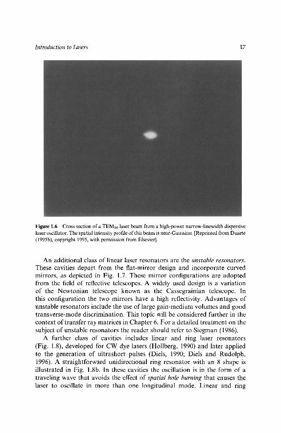
known as the Fresnel number. Here, w is the beam waist at the gain region, L is the length of the cavity, and A is the wavelength of emission. The lower this number, the better the beam quality of the emission or the closer it will be to a single transverse mode, designated by TEM00. A TEM00 is a clean beam with no spatial structure on it, as shown in Fig. 1.6, and is generally round with a near-Gaussian intensity profile in the spatial domain. Thus, long lasers with relatively narrow beam waists tend to yield single-transverse- mode emission. As it will be examined in Chapters 4 and 7, an important part of laser cavity design consists in optimizing the dimensions of the beam waist to the cavity length to obtain TEM00 emission and low beam diver- gences in compact configurations.
Introduction to Lasers 17
Figure 1.6 Cross section of a TEM00 laser beam from a high-power narrow-linewidth dispersive laser oscillator. The spatial intensity profile of this beam is near-Gaussian. [Reprinted from Duarte (1995b), copyright 1995, with permission from Elsevier].
An additional class of linear laser resonators are the unstable resonators. These cavities depart from the flat-mirror design and incorporate curved mirrors, as depicted in Fig. 1.7. These mirror configurations are adopted from the field of reflective telescopes. A widely used design is a variation of the Newtonian telescope known as the Cassegrainian telescope. In this configuration the two mirrors have a high reflectivity. Advantages of unstable resonators include the use of large gain-medium volumes and good transverse-mode discrimination. This topic will be considered further in the context of transfer ray matrices in Chapter 6. For a detailed treatment on the subject of unstable resonators the reader should refer to Siegman (1986).
A further class of cavities includes linear and ring laser resonators (Fig. 1.8), developed for CW dye lasers (Hollberg, 1990) and later applied to the generation of ultrashort pulses (Diels, 1990; Diels and Rudolph, 1996). A straightforward unidirectional ring resonator with an 8 shape is illustrated in Fig. 1.8b. In these cavities the oscillation is in the form of a traveling wave that avoids the effect of spatial hole burning that causes the laser to oscillate in more than one longitudinal mode. Linear and ring

18 Tunable Laser Optics
Figure 1.7 Basic unstable resonator laser cavity.
resonators incorporating saturable absorbers are depicted in the ultrashort pulse cavity configurations of Fig. 1.9. In the ring laser, a collision between two counterpropagating pulses occurs at the saturable absorber. This collision causes the two pulses to interfere, thus creating a transient grating that shortens the emission pulse. This effect is known as colliding-pulse-mode (CPM) locking (Fork etal., 1981). The prisms in this cavity are deployed to provide negative dispersion and thus help in pulse compression, as will be described in Chapter 4.
Dye Jet
CW Laser v ~ M 1 Pump ~ M p
Dispersive and/or FSE
M3
(a)
Dispersive and/or FSE UDD
M3Lj M4
CW Laser .. I - /~~ '~ " - . . .~D__ Pum.
Dye~ jet .""~ Mp (b)
Figure 1.8 (a) Linear and (b) unidirectional 8-shape ring dye laser cavities. [Reprinted from Hollberg (1990), copyright 1990, with permission from Elsevier].

Introduction to Lasers 19
Pump laser
M1
medium
Pulse compressor
M4
le absorber
/ <,./ M 3 (a)
M7
Pump laser Pulse compressor
Gain medium
M2
M1 M4
"•M6 u~ible absorber
M3 (b)
Figure 1.9 (a) Linear femtosecond laser cavity. (b) Ring femtosecond laser resonator. Both laser configurations include a saturable absorber and a multiple-prism pulse compressor.
20 Tunable Laser Optics
Although originally developed for dye lasers, these cavities are widely used with a variety of gain media.
Although most lasers do need efficient and well-designed optical resonators, some lasers have such high gain factors that they tend to emit laserlike radiation, sometimes called superradiant emission or superfluorescence, with only one mirror or even without external mirrors. This means that the intrinsic reflection factors from flat windows provide the necessary feedback for powerful emission, albeit with poor coherence properties. More specifically, this emission tends to be broadband and highly divergent. One additional advantage of using inclined windows when using high-gain laser media is to reduce parasitic reflections that tend to contribute to output noise. Some laser media that produce very high gains include copper vapor, molecular nitrogen, and laser dyes.
PROBLEMS
1. Show that in the steady state, Eq. (1.14) becomes Eq. (1.18). 2. Show that in the steady state, Eq. (1.17) becomes Eq. (1.21). 3. Show that by neglecting the triplet state, Eq. (1.21) can be expressed as
Eq. (1.23). 4. Starting from Eqs. (1.39) and (1.40), derive an expression for [DII 2 and
show that it is equal to IDII] 2. 5. Use Eq. (1.49) to arrive at the expression for the transition cross section
given in Eq. (1.50).
REFERENCES
Byer, R. L., Herbst, R. L., Kildal, H., and Levenson, M. D. (1972). Optically pumped molecular iodine vapor-phase laser. Appl. Phys. Lett. 20, 463-466.
Chutjian, A., and James, T. C. (1969). Intensity measurements in the B 3 II u +-X1Ng+ system of I2. J. Chem. Phys. 51, 1242-1249.
Diels, J.-C. (1990). Femtosecond dye lasers. In Dye Laser Principles (Duarte, F. J., and Hillman, L. W., eds.). Academic Press, New York, pp. 41-132.
Diels, J.-C., and Rudolph, W. (1996). Ultrashort Laser Pulse Phenomena. Academic Press, New York.
Dienes, A., and Yankelevich, D. R. (1998). Tunable dye lasers. In Encyclopedia of Applied Physics, Vol. 22 (Trigg, G. L., ed). Wiley-VCH, New York, pp. 299-334.
Dirac, P. A. M. (1978). The Principles of Quantum Mechanics, 4th ed. Oxford University Press, London.
Duarte, F. J. (1990a). Narrow-linewidth pulsed dye laser oscillators. In Dye Laser Principles (Duarte, F. J., and Hillman, L. W., eds.) Academic Press, New York, pp. 133-183.

Introduction to Lasers 21
Duarte, F. J. (1990b). Technology of pulsed dye lasers. In Dye Laser Principles (Duarte, F. J., and Hillman, L. W., eds.). Academic Press, New York, pp. 239-285.
Duarte, F. J. (1995a). Dye lasers. In Tunable Lasers Handbook (Duarte, F. J., ed.). Academic Press, New York, pp. 167-218.
Duarte, F. J. (1995b). Solid-state dispersive dye laser oscillator: very compact cavity. Opt. Commun. 117, 480-484.
Duarte, F. J. (1998). Interference of two independent sources. Am. J. Phys. 66, 662-663. Dujardin, G., and Flamant, P. (1978). Amplified spontaneous emission and spatial dependence
of gain in dye amplifiers. Opt. Commun. 24, 243-247. Everett, P. N. (1991). Flashlamp-excited dye lasers. In High-Power Dye Lasers (Duarte, F. J.,
ed.). Springer-Verlag, Berlin, pp. 183-245. Feynman, R. P., Leighton, R. B., and Sands, M. (1965). The Feynman Lectures on Physics,
Vol. III, Addison-Wesley, Reading, MA. Fork, R. L., Greene, B. I., and Shank, C. V. (1981). Generation of optical pulses shorter than
0.1 psec by colliding pulse-mode locking, Appl. Phys. Lett. 38, 671-672. Ganiel, U., Hardy, A., Neumann, G., and Treves, D. (1975). Amplified spontaneous emission
and signal amplification in dye-laser systems. IEEE J. Quantum Electron. QE-11, 881-892. Haag, G., Munz, M., and Marowski, G. (1983). Amplified spontaneous emission (ASE) in laser
oscillators and amplifires. IEEE J. Quantum Electron. QE-19, 1149. Haken, H. (1970). Light and Matter. Springer-Verlag, Berlin. Hammond, P. (1979). Spectra of the lowest excited singlet states of rhodamine 6G and rhoda-
mine B. IEEE J. Quantum Electron. QE-15, 624-632. Hargrove, R. S., and Kan, T. K. (1980). High-power efficient dye amplifier pumped by copper
vapor lasers. IEEE J. Quantum Electron. QE-16, 1108-1113. Hillman, L. W. (1990). Laser dynamics. In Dye Laser Principles (Duarte, F. J., and Hillman, L. W.,
eds.). Academic Press, New York, pp. 17-39. Hollberg, L. (1990). CW dye lasers. In Dye Laser Principles (Duarte, F. J., and Hillman, L. W.,
eds.). Academic Press, New York, pp. 185-238. Javan, A., Benett, W. R., and Herriott, D. R. (1961). Population inversion and continuous optical
maser oscillation in a gas discharge containing a He-Ne mixture. Phys. Rev. Lett. 6, 106-110. Jensen, C. (1991). Pulsed dye laser gain analysis and amplifier design. In High-Power Dye Lasers
(Duarte, F. J., ed.). Springer-Verlag, Berlin, pp. 45-91. Maiman, T. H. (1960). Stimulated optical radiation in ruby. Nature 187, 493-494. Munz, M., and Haag, G. (1980). Optimization of dye-laser output coupling by consideration of
the spatial gain distribution. Appl. Phys. 22, 175-184. Nair, L. G., and Dasgupta, K. (1985). Amplified spontaneous emission in narrow-band pulsed
dye laser oscillators--theory and experiment. IEEE J. Quantum Electron. 21, 1782-1794. Penzkofer, A., and Falkenstein, W. (1978). Theoretical investigation of amplified spontaneous
emission with picosecond light pulses in dye solutions. Opt. Quantum Electron. 10, 399-423.
Peterson, O. G. (1979). Dye lasers. In Methods of Experimental Physics, Vol. 15 (Tang, C. L., ed.). Academic Press, New York, pp. 251-359.
Sargent, M., Scully, M. O., and Lamb, W. E. (1974). Laser Physics, Addison Wesley, Reading, MA. Sch~fer, F. P. (ed.). (1990). Dye Lasers, 3rd ed. Springer-Verlag, Berlin. Sch~ifer, F. P., Schmidt, W., and Volze, J. (1966). Organic dye solution laser. Appl. Phys. Lett. 9,
306-309. Siegman, A. (1986). Lasers. University Science Books, Mill Valley, California. Silfvast, W. T. (1996). Laser Fundamentals. Cambridge University Press, Cambridge, UK. Sorokin, P. P., and Lankard, J. R. (1966). Stimulated emission observed from an organic dye,
chloro-aluminum phthalocyanine. IBM J. Res. Dev. 10, 162-163.

22 Tunable Laser Optics
Teschke, O., Dienes, A., and Whinnery, J. R. (1976). Theory and operation of high-power CW and long-pulse dye lasers. IEEE J. Quantum Electron. QE-12, 383-395.
Tuccio, S. A., and Strome, F. C. (1972). Design and operation of a tunable continuous dye laser. Appl. Opt. 11, 64-73.
Webb, J. P., McGolgin, W. C., Peterson, O. G., Stockman, D. L., and Eberly, J. H. (1970). Intersystem crossing rate and triplet state lifetime for a lasing dye. J. Chem. Phys. 53, 4227-4229.
Willett, C. S. (1974). An introduction to Gas Lasers: Population Inversion Mechanisms. Pergamon Press, New York.

Chapter 2
Dirac Optics
2.1 DIRAC NOTATION IN OPTICS
Dirac discussed in his classic book Principles of Quantum Mechanics, first published in 1930 (Dirac, 1978), the essence of interference as a one-photon phenomenom. He did so, however, qualitatively. In 1965 Feynman discussed electron interference in two-slit thought experiments using probability amplitudes and Dirac's notation as a tool (Feynman etal., 1965a). In 1991 Dirac's notation was applied to the propagation of coherent light in an N-slit interferometer (Duarte, 1991).
The concept behind the notation invented by Dirac can be explained by considering the propagation of a particle from plane s to plane x, as illustrated in Fig. 2.1. According to the Dirac concept there is a probability amplitude, denoted by Ixls), that quantifies such propagation. Historically, Dirac intro- duced the nomenclature of ket vectors, denoted by ]), and bra vectors, denoted by (], which are mirror images of each other. Thus the probability amplitude is described by the braket (x]s), which is a complex number.
It is important to note that in Dirac's notation the propagation from s to x is expressed in reverse by Ix[s). In other words, the starting condition is at the right and the final condition is at the left. If the propagation of the photon is not directly from plane s to plane x, but involves the passage through an intermediate plane j, as illustrated in Fig. 2.2, then the prob- ability amplitude describing such propagation is
(x[s) = (xlj) (jls) (2.1)
23

24 Tunable Laser Optics
S x
Figure 2.1 Propagation from plane s to plane x is expressed as (xls).
If the photon from plane s must also propagate through planes j and k in its trajectory to plane x, as illustrated in Fig. 2.3, then the probability amplitude is given by
(xls) - (xlk) (k l j ) ( j s) (2.2)
When at the intermediate plane in Fig. 2.2, a number of N alternatives are available to the passage of the photon, as depicted in Fig. 2.4a, then the overall probability amplitude must consider every possible alternative, which is expressed mathematically by a summation over j in the form of
N
<xls> - F_~ <xlj><jls> (2.3) j = l
s 1 x
Figure 2.2 Propagation from plane s to plane x via an intermediate planej is expressed as (x]j) (j[s).
s 1 k x
Figure 2.3 Propagation from plane s to plane x via two intermediate planesj and k is expressed as (x k)(k j)(jls).

Dirac Optics 25
(a)
(b) s
1 1
1
k x
Figure 2.4 (a) Propagation from plane s to plane x via an array of N-slits positioned at the intermediate plane j. (b) Propagation from s to x via an array of N-slits positioned at the intermediate plane j and via an additional array of N-slits positioned at k.
For the case of an additional intermediate plane with N alternatives, as illustrated in Fig. 2.4b, the probability amplitude is written as
N N
(xls) - ~ ~ (xlk)(klj)( j]s) (2.4) k--1 j=l
The addition of further intermediate planes, with N alternatives, can then be systematically incorporated in the notation. The Dirac notation, though originally applied to the propagation of single particles (Dirac, 1978; Feyn- man et al., 1965a), also applies to describing the propagation of ensembles of coherent, or indistinguishable, photons (Duarte 1991, 1993). This is in agreement with the interpretation that suggests that the principles of quan- tum mechanics are applicable to the description of macroscopic phenomena that are not perturbed by observation (van Kampen, 1988).
2.2 I N T E R F E R E N C E
As outlined by Feynman in his thought experiments on two-slit electron interference, Dirac's notation offers a natural avenue to describe the propa- gation of particles from a source to a detection plane via a pair of slits. This idea can be extended to the description of photon propagation from a source s to a screen detector x via a transmission grating j comprising N slits, as illustrated in Fig. 2.5.
26 Tunable Laser Optics
I Telescope
Multiple-prism beam
expander
----', 1
, 3', I
I I
I I
I I !
! !
I ! i !
I !
J x S
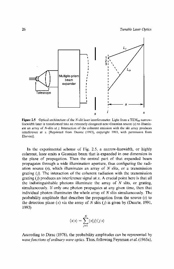
Figure 2.5 Optical architecture of the N-slit laser interferometer. Light from a TEM00 narrow- linewidth laser is transformed into an extremely elongated near-Gaussian source (s) to illumin- ate an array of N-slits at j. Interaction of the coherent emission with the slit array produces interference at x. [Reprinted from Duarte (1993), copyright 1993, with permission from Elsevier].
In the experimental scheme of Fig. 2.5, a narrow-linewidth, or highly coherent, laser emits a Gaussian beam that is expanded in one dimension in the plane of propagation. Then the central part of that expanded beam propagates through a wide illumination aperture, thus configuring the radi- ation source (s), which illuminates an array of N slits, or a transmission grating (j). The interaction of the coherent radiation with the transmission grating (j) produces an interference signal at x. A crucial point here is that all the indistinguishable photons illuminate the array of N slits, or grating, simultaneously. If only one photon propagates at any given time, then that individual photon illuminates the whole array of N slits simultaneously. The probability amplitude that describes the propagation from the source (s) to the detection plane (x) via the array of N slits (j) is given by (Duarte, 1991, 1993)
N
<xls) - ~ <xlj) <Jl,> j= l
According to Dirac (1978), the probability amplitudes can be represented by wave functions o f ordinary wave optics. Thus, following Feynman et al. (1965a),
Dirac Optics 27
(jls) - q~(rj,s)e -i~ (2.5)
(xl j ) - q~(rxj)e -i~j (2.6)
Here, Oj and ~bj are the phase terms associated with the incidence and diffraction waves, respectively. Using these expressions for the probability amplitudes then, Eq. (2.3) can be written as
N < x l s > - ~(r j )e -i~' (2.7)
j=l
where
t~(rj) = @(rxj)t~(rj,s) (2.8)
f~j = (Oj + ~by) (2.9)
The propagation probability can be obtained by expanding Eq. (2.7) and multiplying the expansion by its complex conjugate, in other words by performing the multiplication
<X]S) <X]S>* -- ]<X]S> 12 (2.10)
and using the identity
2 cos(Dm - a j ) - e -i(am-a') + e i(am-a') (2.11)
we can write the generalized propagation probability in one dimension
N N I(X[S)[2 -- Z ~(rj)~ ~(rm)e i(9tm-ctj) (2.12)
j=l m=l
which can be expressed as (Duarte and Paine, 1989; Duarte, 1991)
I<xls)l 2 - ~ ~(rj) 2 -+- 2 Z ~(r j ) ~(rm) c o s ( a m -- ~'-~j) (2.13) "= m=j+l
Interference due to transmission in a two-dimensional transmission grating can be described by considering the experimental setup depicted in Fig. 2.6. Propagation occurs from s to x via a two-dimensional transmission grating jzy; that is, j is replaced by a grid comprised ofj components in the y direction and j components in the z direction. Note that in the one-dimen- sional case only the y component ofj is present, which is written simply as j. The plane configured by the jzy grid is orthogonal to the plane of propaga- tion. Hence, for photon propagation from s to x via jzy, the probability amplitude is given by (Duarte, 1995a).

28 Tunable Laser Optics
Figure 2.6 A two-dimensional representation of the (x j ) ( j s) geometry.
N N
/~l,/- Z Z/~lJ~.y//J~, ,/ L=I jy=l
(2.14)
Now, if the j is abstracted from j~y, then Eq. (2.14) can be expressed as
N N
Ixl,I - Z Z , ~ l r z , le-i~:; ' z=l y=l
(2.15)
and the corresponding probability is given by (Duarte, 1995a)
I(xl~)l= N N N N
z=l y=l q=l p=l
(2.16)
For a three-dimensional transmission grating it can be shown that
N N N N N N
z=l y=l x=l q=l p=l r=l
(2.17)
It is important to emphasize that the concepts described here apply to the propagation of single photons and to the propagation of ensembles of

Dirac Optics 29
coherent, &dist&guishable (monochromatic) photons. The application of quantum principles to the description of the propagation of large numbers of monochromatic, or indistinguishable, photons was already advanced by Dirac in his discussion of interference (Dirac, 1978; Duarte, 1998).
2.2.1 GEOMETRY OF THE N-SLIT INTERFEROMETER
In addition to the generalized interferometric equations it is important to consider the geometry of the transmission grating (j) in conjunction with the plane of interference (x) for the one-dimensional case, as illustrated in Fig. 2.7. According to the geometry, the phase-difference term in Eq. (2.13) can be expressed as (Duarte, 1997)
COS( (O m - - Oj) -~ ( r -- r - - COS(l /m - - l m - , I k l • ILm - L m - l l k 2 ) ( 2 . 1 8 )
where
kl = 27rnl/Av (2.19)
k2 = 27rnz/Av (2.20)
are the wavenumbers of the two optical regions defined in Fig. 2.7b. Here, A1 = Av/nl and/~2 - - )~v/n2, where Av is the vacuum wavelength and nl and n2 are the corresponding indexes of refraction (Wallenstein and Hfinsch, 1974; Born and Wolf, 1999). The phase differences can be expressed exactly via the following geometrical equations (Duarte, 1993):
Itm - t m - l l = 2~mdm/ltm -+- t m - l l
L 2 - a 2 + (~m + (dm/2)) 2
2 __ a 2 2 t m _ l + (~m - ( d m / 2 ) )
(2.21)
(2.22)
(2.23)
In this notation, ~m is the lateral displacement on the x plane, from the projected median of dm to the interference plane.
2.2.2 N-SLIT INTERFEROMETER EXPERIMENT
The N-slit interferometer is illustrated in Fig. 2.5. In practice this interfe- rometer can be configured with a variety of lasers, including tunable lasers. However, one requirement is that the laser to be utilized emit in the narrow- linewidth regime and in a single transverse mode (TEM00) with a near- Gaussian profile. Ideally the source should be a single-longitudinal-mode

30 Tunable Laser Optics
\\ / Lm
~m k2, n2
(a)
d~
,, a ,
~m
dm/2
/I",,, / ',, o~ i ~ ; -
/ 'gml \
k ~ , ~ l k2' n2
(b) I 1
Figure 2.7 (a) Detailed perspective of the transmission grating plane (j) and the detection plane (x) including the relevant geometrical parameters. (b) The grating plane (j) depicting the difference in path length and the angles of incidence (Om) and diffraction (~m) for the condition a >> din. (From Duarte, 1997.)

Dirac Optics 31
laser. The reason for this requirement is that narrow-linewidth lasers yield sharp, well-defined interference patterns close to those predicted theoret- ically for a single wavelength.
One particular configuration of the N-slit interferometer can be integrated by a TEM00 He-Ne laser (A ~ 632.8 nm) with a beam 0.5 mm in diameter. It should be emphasized that this class of laser yields smooth near-Gaussian beam profiles and narrow-linewidth emission. The laser beam is then magnified, in two-dimensions, by a • 20 Galilean telescope. Following the telescopic expan- sion the beam is further expanded, in one dimension, by a • 5 multiple-prism beam expander. This optical arrangement yields an expanded smooth near- Gaussian beam approximately 50 mm wide. An option is to insert a convex lens prior to the multiple-prism expander. This produces an extremely elongated near-Gaussian beam 20-30~tm at it maximum height by 50mm in width (Duarte, 1993). The beam propagation through this system can be accurately characterized using ray transfer matrices, as discussed in Chapter 6 (Duarte, 1995b). Also, as an option, at the exit of the multiple-prism beam expander an aperture, a few mm wide, can be deployed. Thus, the source s can be either the exit prism of the multiple-prism beam expander or the wide aperture.
At this stage it should be noted that for the illumination of two slits 50 lam in width that are separated by 501am, the elongated Gaussian provides a nearly plane illumination. That is also approximately the case even if a larger number of slits of these dimensions are illuminated. For the particular case of a two-slit experiment, or Young's interference experiment, involving 50- ~tm slits separated by 50 ~tm and a grating-to-screen distance (a) of 10 cm, the interference signal is displayed in Fig. 2.8a. The calculated interference using Eq. (2.13) and assuming plane-wave illumination is given in Fig. 2.8b. The interference screen at x is a digital detector comprising an array of photo- diodes, each 25 ~tm in width. For an array of 100 slits, each 30 ~tm in width and separated by 30 ~m, the measured and calculated interferograms are shown in Fig. 2.9. Here the grating-to-digital-detector distance is a = 75 cm.
In practice the transmission gratings are not perfect and offer an uncer- tainty in the dimension of the slits. The uncertainty in the slit dimensions of the grating, incorporating the 30~tm slits used in this experiment was measured to be 2% or less. The theoretical interferogram for the grating comprising by 100 slits, each 30.0+0.6~tm wide and separated by 30.0 + 0.6 ~tm, is given in Fig. 2.10. Notice the symmetry deterioration.
When a wide slit is used to select the central portion of the elongated Gaussian beam, the interaction of the coherent laser beam with the slit results in diffraction prior to the illumination of the transmission grating. The interferometric Eq. (2.13) can be used to characterize this diffraction. This is done by dividing the wide slit into hundreds of smaller slits. As an example, a 3-mm-wide aperture is divided into 600 slits, each 4 ~tm wide and

2.0
Tunable Laser Optics
~, 14~176176 _F
"~- 10000 -
E
=_, oooo A / / A
n- 2000
%od;Oo,,,x~
1.6
(b)
"~ 1.2 - e,,
~: 08
0.0 ~ ~ , i -20.0 -10.0 0.0 10.0 20.0 S c r e e n A x i a l D i s t a n c e ( m e t e r s ) x 10 4
0.4
32
Figure 2.8 (a) Measured interferogram resulting from the interaction of coherent laser emission at )~--632.82 nm and two slits 50 pm wide, separated by 50 pm. The j to x distance is 10cm. (b) Corresponding theoretical interefogram from Eq. (2.13). Note: the horizontal axis in this figure is referred to as the Screen Axial Distance. This is the axis on the screen x which is orthogonal to the axis of propagation [From Duarte (1991), copyright 1991, with permission from Springer-Verlag].
separated by a 1-1am interslit distance. The calculated near-field diffraction pattern for a distance of 10cm is shown in Fig. 2.11. Using this class of radiation source to illuminate the 100-slit grating comprising 30 pm slits with an interslit distance of 30 pm (for a = 75 cm) yields the theoretical interfero- gram displayed in Fig. 2.12.
2.3 DIFFRACTION
Feynman, in his usual style, stated that no one has ever been able to define the difference between interference and diffraction satisfactorily (Feynman

Dirac Optics 33
7000 i .,,= ~= "-' 5000
.>_ .
( a ) ' ' 'r 100 300 500 700 900
N u m b e r of P ixe ls
14.0
12.0
10.0
c 8.0 ~=
, , . , . , .
.> 6.0 u
rr 4.0
2.0-
.0 -0.0100 -0.0050 0.0000 0.0050 0.0100
(b) Screen Axial Distance (meters)
Figure 2.9 (a) Measured interferogram resulting from the interaction of coherent laser emis- sion at A - 632.82 nm and 100 slits, 30 gm wide and separated by 30 gm. The j-to-x distance is 75cm. (b) Corresponding theoretical interefogram from Eq. (2.13). [Reprinted from Duarte (1993), copyright 1993, with permission from Elsevier].
etal., 1965b). His point is well taken. In the discussion related to Fig. 2.9 and its variants, reference was only made to interference. However, what we really have is interference in three diffraction orders. That is, the 0th, or central, order and the +1, or secondary, orders. In other words, there is an interference pattern associated with each diffraction order. Phys- ically, however, this is the same phenomenon. The interaction of coherent

34 Tunable Laser Optics
14.0
12.0
10.0
t~ r 8.0 c Q
6.0
0
4.0
2.0
0.0 r -ls.o '-~d.o ' - s l o ' 6 ' ~g.o
1 \ s ' ~ c ; o '
Screen Axial Distance (meters) x 10 -a Figure 2.10 Theoretical interfererometric/diffraction distribution using a _<2% uncertainty in the dimensions of the 30-~tm slits. In this calculation, N = 100 and the j-to-x distance is 75 cm. A deterioration in the spatial symmetry of the distribution is evident. [Reprinted from Duarte (1993), copyright 1993, with permission from Elsevier].
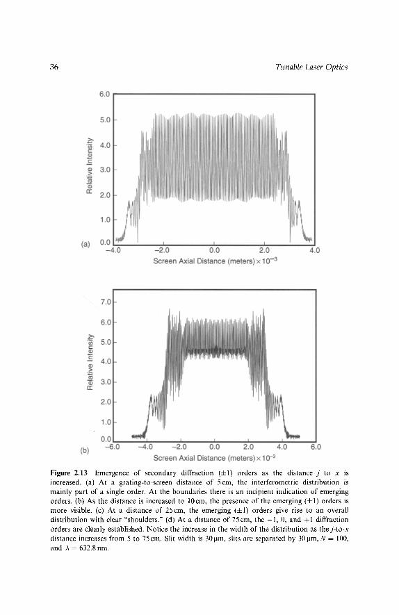
light with a set of slits in the near field gives rise to an interference pattern. As the distance a from j to x increases, the central interference pattern begins to give rise to secondary patterns that gradually separate from the central order at lower intensities. These are the +1 diffraction orders. This physical phenomenon as one goes from the near to the far field is illustrated in Fig. 2.13. One of the beauties of the Dirac description of optics is the ability to move continuously from the near to the far field with a single mathematical description.
The second interference-diffraction entanglement refers to the fact that our generalized interference equation can be naturally applied to describe a diffraction pattern produced by a single wide slit, as shown in Fig. 2.11. Under those circumstances the wide slit is mathematically represented by a series of subslits.

Dirac Optics 35
7.0
6 . 0 -
_>, 5 . 0 - t/} t - O E 4 . 0 -
.>_ 3 . 0 -
tr
2 . 0 -
1 . 0 -
0.0 -3.0
__j I I I I I
- 2 o -1 o o o l o 2 o Screen Axial Distance (meters) x 10 -3
3.0
Figure 2.11 Theoretical interferometric distribution produced by a 3 mm aperture illuminated at A = 632.82 nm. The j to x distance is 10 cm.
1.0.
0.8
"~ 0 6 ' c--
=> 0.4-
rc
0.2
| I | | | | | |
-12.5 -7.5 -2.5 0 2.5 7.5 12.5
Screen Axial Distance (meters) x 10 -3
Figure 2.12 Theoretical interferometric distribution incorporating diffraction-edge effects in the illumination. In this calculation the slits in the array are 30Hm wide and separated by 30~tm, N - 1 0 0 , and the j-to-x distance is 75cm. The aperture-grating distance is 10cm. [Reprinted from Duarte (1993), copyright 1993, with permission from Elsevier].
36 Tunable Laser Optics
Figure 2.13 Emergence of secondary diffraction (+1) orders as the distance j to x is increased. (a) At a grating-to-screen distance of 5cm, the interferometric distribution is mainly part of a single order. At the boundaries there is an incipient indication of emerging orders. (b) As the distance is increased to 10cm, the presence of the emerging (+1) orders is more visible. (c) At a distance of 25cm, the emerging (+1) orders give rise to an overall distribution with clear "shoulders." (d) At a distance of 75cm, the -1 , 0, and +1 diffraction orders are clearly established. Notice the increase in the width of the distribution as the j-to-x distance increases from 5 to 75 cm. Slit width is 30 lam, slits are separated by 30 ~tm, N = 100, and A = 632.8 nm.
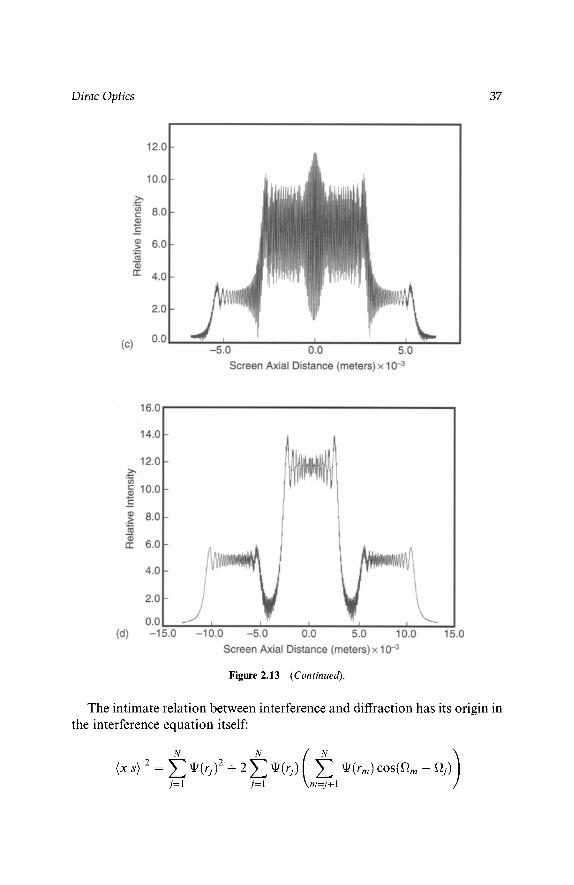
Dirac Optics 37
Figure 2.13 (Continued).
The intimate relation between interference and diffraction has its origin in the interference equation itself:
N N )

38 Tunable Laser Optics
for it is the COS(~-~m- ~-~j) term that gives rise to the different diffraction orders.
From the geometry of Fig. 2.7 we can write
sin ff~m -- (~m + (dm/2))/Lm (2.24)
And for the condition a >> din, we have ILm-k-Lm-ll ,-~ 2Lm. Then using Eqs. (2.21) and (2.24) we have
]Lm - Lm-1] ~ dm sin ff~m (2.25)
]lm -- lm-l l ~ dm sin ~)m (2.26)
where Om and (~)m are the angles of incidence and diffraction, respectively. Given that maxima occur at
([lm -- lm-1 Inl -+-ILm - Lm-1 ]nz)ZTr/Av = MTr (2.27)
then, using Eqs. (2.25) and (2.26), we get
dm(nl sin Om + n2 sin ff~m)(27r/Av) = MTr (2.28)
where M = 0, 2, 4, 6 , . . . . For nl = n2 we have A = Av, and this equation reduces to the well-known diffraction grating equation
dm(sin Om+ sin ff~m) = mA (2.29)
where m = 0, 1, 2, 3 , . . . are the various diffraction orders.
2.4 REFRACTION
An additional fundamental phenomenon in optics is refraction. This is the change in the geometrical path of a beam of light due to transmission from the original medium of propagation to a second medium with a different refractive index. For example, refraction is the bending of a ray of light due to propagation in a glass or crystalline prism.
If in the diffraction grating equation dm is made very small relative to a given A, diffraction ceases to occur and the only solution that can be found is for m = 0. That is, under these conditions a grating made of grooves coated on a transparent substrate, such as optical glass, does not diffract and exhibits the refraction properties of the glass. For example, since the maximum value of ( sin ~:)m -+- sin ff~m) is 2 for a 5000-1ines/mm transmission grating, no diffraction can be observed for the visible spectrum. Hence for the condition dm << A, the diffraction grating equation can only be solved for
din(n1 sin Om 4- n2 sin ff)m)(27r/Av) = 0 (2.30)

Dirac Optics 39
which can lead to
rtl sin Om -- rt2 sin ~m (2.31)
For an air-glass interface, n l = 1 and
sin Om = n2 sin ~)m (2.32)
which is the well-known equation of refraction, also known as Snell's law. Under the present physical conditions, ~m is the angle of incidence and ffm becomes the angle of refraction.
2.5 R E F L E C T I O N
Up to now, the discussion on interference has involved an N-slit array, or a transmission grating. It should be indicated that the arguments and physics apply equally well to a reflection interferometer, that is, to an interferometer incorporating a reflection, rather than a transmission, grat- ing. Explicitly, if a mirror is placed at an infinitesimal distance immediately behind the N-slit array of Fig. 2.7, as illustrated in Fig. 2.14, then the interferometer becomes a reflection interferometer. Under those circum- stances the equations
dm(nl sin Om • n2 sin ~m)(27r/)~v) = MTr and dm(sin {~)m ~ sin (I)m) = mA
'\\
N-slit array,, 0 / % \\
Figure 2.14 A reflection diffraction grating is formed by approaching a reflection surface at an infinitesimal distance to the array of N slits.

40 Tunable Laser Optics
apply in the reflection domain, with {~m being the incidence angle and (I)m the diffraction angle in the reflection domain. For the case of dm << A and nl = n2, we can then have
sin Om -- sin (I) m (2.33)
which means
Om = (I)m (2.34)
where E)m is the angle of incidence and (I)m is the angle of reflection. This is known as the law of reflection.
2.6 A N G U L A R DISPERSION
Angular dispersion, an important quantity in optics, describes the ability of an optical element, such as a diffraction grating or prism, to geometrically spread a beam of light as a function of wavelength. Mathematically it is expressed by the differential (00/0A). For spectrophotometers and wave- length meters based on dispersive elements, such as diffraction gratings and prism arrays, the dispersion should be as large as possible since that enables a higher-wavelength spatial resolution. Further, in the case of dispersive laser oscillators, a high dispersion leads to the achievement of narrow-linewidth emission, since the dispersive linewidth is given by (see Chapter 3)
A~ ~ AO(OO/O)k) -1 (2.35)
where (00/0A) is the overall intracavity dispersion. For a uniform diffraction grating, dm = d and the grating equation
becomes
d(sin 0 + sin ~) = mA (2.36)
The angular dispersion is calculated by differentiating Eq. (2.36), so
(O0/OA) = m/ (d cos O) (2.37)
or alternatively
(00/0A) = (sinO-t- sin ~)/(A cos O) (2.38)
For a prism deployed at minimum deviation, as illustrated in Fig. 2.15, the following set of geometrical relations apply:
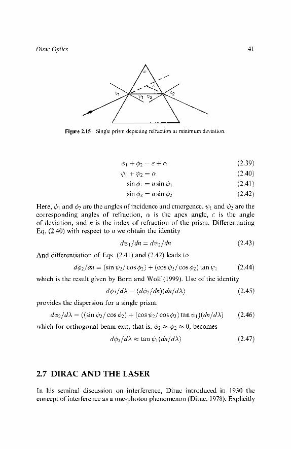
Dirac Optics
1 /
Figure 2.15 Single prism depicting refraction at minimum deviation.
41
q~l -~- q~2 = C -+- O~ (2.39)
~;1 -Jr- ~2 = Ol (2.40) sin 4~1 = n sin ~1 (2.41)
sin ~2 = t / s in ~;2 (2.42)
Here, ~1 and ~2 are the angles of incidence and emergence, ~1 and ff;2 are the corresponding angles of refraction, c~ is the apex angle, c is the angle of deviation, and n is the index of refraction of the prism. Differentiating Eq. (2.40) with respect to n we obtain the identity
d~l/dn = d~z/dn (2.43)
And differentiation of Eqs. (2.41) and (2.42) leads to
d~z/dn = (sin ~;2/COS q~2) -+- (COS if;Z/COS ~2) tan ~1 (2.44)
which is the result given by Born and Wolf (1999). Use of the identity
d~z/dA = (d~z/dn)(dn/dA) (2.45)
provides the dispersion for a single prism,
d~z/dA = ((sin ~2/COS q~2) -+- (COS if)Z/COS ~2) tan ~l)(dn/dA) (2.46)
which for orthogonal beam exit, that is, ~2 ~ ~;2 "~ 0, becomes
d~z/dA ~ tan ~l (dn/dA) (2.47)
2.7 DIRAC A N D THE LASER
In his seminal discussion on interference, Dirac introduced in 1930 the concept of interference as a one-photon phenomenon (Dirac, 1978). Explicitly

42 Tunable Laser Optics
he stated: Each photon then interferes only with itself. Interference between two different photons never occurs. This concept is central to explaining the physics of the N-slit interferometer, since it is a single photon that illuminates the whole the array of N slits, or the grating, simultaneously. In the case of a monochromatic laser beam, that is, an ensemble of indistinguishable photons, all the indistinguishable photons illuminate the array of N slits, or the grating, simultaneously. In the past this concept has been the source of some controversy due to a misunderstanding of the Dirac interpretation that implies that indistinguishable photons, regardless of source of origin, are the same photon. On the other hand, distinguishable photons, or photons of different wavelengths, do not interfere with each other.
The Dirac discussion on the interference of photons goes even further. It begins with reference to a beam of roughly monochromatic light; then, prior to his dictum on interference, he writes about a beam of light having a large number of photons. It is this beam of light that in his discussion is divided into two components and is subsequently made to interference. In present terms this is no different than the description of interference due to the interaction of a high-power narrow-linewidth laser beam with a two-beam interferometer (Duarte, 1998). In other words, in 1930 Dirac provided perhaps the earliest physical description of a laser beam.
PROBLEMS
1. Show that substitution of Eqs. (2.5) and (2.6) into Eq. (2.3) leads to Eq. (2.7).
2. Show that Eq. (2.12) can be expressed as Eq. (2.13). 3. From the geometry of Fig. 2.7 derive Eqs. (2.21)-(2.23). 4. Write an equation for I< x[s >12 in the case relevant to Fig. 2.12, that is,
an N-slit grating illuminated by a single wide slit. Assume that the single wide slit can be represented by an array of N subslits.
5. Show that, for orthogonal beam exit, Eq. (2.46) reduces to Eq. (2.47).
REFERENCES
Born, M., and Wolf, E. (1999). Principles of Optics, 7th ed. Cambridge University Press, New York.
Dirac, P. A. M. (1978). The Principles of Quantum Mechanics, 4th ed. Oxford University Press, London.
Duarte, F. J. (1991). Dispersive dye lasers. In High Power Dye Lasers (Duarte, F. J., ed.). Springer-Verlag, Berlin, pp. 7-43.

Dirac Optics 43
Duarte, F. J. (1993). On a generalized interference equation and interferometric measurements. Opt. Commun. 103, 8-14.
Duarte, F. J. (1995a). Interferometric imaging. In Tunable Laser Applications (Duarte, F. J., ed.). Marcel Dekker, New York, pp. 153-178.
Duarte, F. J. (1995b). Narrow-linewidth laser oscillators and intracavity dispersion. In Tunable Lasers Handbook (Duarte, F. J., ed.). Academic Press, New York, pp. 9-32.
Duarte, F. J. (1997). Interference, diffraction, and refraction, via Dirac's notation. Am. dr. Phys. 65, 637-640.
Duarte, F. J. (1998). Interference of two independent sources. Am. J. Phys. 66, 662-663. Duarte, F. J., and Paine, D. J. (1989). Quantum mechanical description of N-slit interference
phenomena. In Proceedings of the International Conference on Lasers '89 (Harris, D. G., and Shay, T. M., eds.). STS Press, McLean, VA, pp. 42-27.
Feynman, R. P., Leighton, R. B., and Sands, M. (1965a). The Feynman Lectures on Physics, Vol. III, Addison-Wesley, Reading, MA.
Feynman, R. P., Leighton, R. B., and Sands, M. (1965b). The Feynman Lectures on Physics, Vol. I, Addison-Wesley, Reading, MA.
Van Kampen, N. G. (1988). Ten theorems about quantum mechanical measurements. Physica A 153, 97-113.
Wallenstein, R., and H~insch, T. W. (1974). Linear pressure tuning of a multielement dye laser spectrometer. Appl. Opt. 13, 1625-1628.

This Page Intentionally Left Blank

Chapter 3
The Uncertainty Principle in Optics
3.1 APPROXIMATE DERIVATION OF THE UNCERTAINTY PRINCIPLE
The uncertainty principle is of fundamental importance to optics and to laser optics in particular. Here, optical arguments are applied to outline an approximate derivation of the uncertainty principle.
3.1.1 THE WAVE CHARACTER OF PARTICLES
The quantum energy of a particle is given by the well-known quantum energy equation
E = h v (3.1)
where h is Planck's constant. Equating this to the relativistic energy equation E = m c 2 and using the identity )~ = c/u, an expression for the momentum of a particle can be given as
p = h / k (3.2)
which, using the identity
k = 27r/k (3.3)
45

46 Tunable Laser Optics
can be restated as
p = hk (3.4)
This momentum equation was applied to particles, such as electrons, by De Broglie (Haken, 1981). Thus, wave properties such as frequency and wavelength were attributed to the motion of particles.
3 .1 .2 THE DIFFRACTION IDENTITY AND THE UNCERTAINTY
PRINCIPLE
In his discussion of position and momentum, Feynman (Feynman et al., 1965) considers the relative uncertainty in the wavelength that can be meas- ured with a given grating. Using that approach he arrives at an expression for the resolving power of a diffraction grating, namely, AA/A. His discus- sion is then extended to include the length of a wave train in order to derive an identity for AA/A 2. Here, the origin of this expression is examined from an interferometric perspective.
The generalized one-dimensional interferometric equation derived using Dirac's notation is given by (Duarte, 1991)
I(xts)l 2 = ~ ~ ( r j ) 2 -+- 2 ~ tI,(rj) ~ ( r m ) c o s ( a m - Qj) (3.5) j=l j=l m=j+l
The interference term in this equation can be expressed as (Duarte, 1997)
COS((0 m -- Oj) -Jr" ((~m -- ~ j ) ) - - COS(I/m -- /m-11kl -'}- ILm - t m - 1 1 k 2 ) (3.6)
where k l - 2rml/Av and k 2 - 2rm2/Av are the wave numbers for the two optical regions defined in Fig. 3.1. Also, Ilm - lm-l[ and ILm - Lm-l] are the corresponding path differences. Since it can be shown that m a x i m a can occur at
([lm -- lm-1 ]nl -4-]tm - t m - 1 ]n2)2rC/Av = Mrc (3.7)
where M = 0, + 2, + 4, + 6 , . . . , then it can be shown that
dm(?'ll sin {~m 4-//2 sin ~m)2rr/Av -- Mrr (3.8)
which, for nl = n2 = 1 and A -- A~, reduces to
dm(sin {~m --1-- sin '~m)k = Mrr (3.9)
which can be expressed as the well-known grating equation,
din(sin Om+ sin Ore) = mA (3.10)

The Uncertainty Principle in Optics 47
/
k~ k2, n2
Figure 3.1 Region boundary, for kl and k2, at the plane j. (From, Duarte, 1997.)
where m = 0, + 1, + 2, + 3,. . . . . For a grating deployed in the reflection domain and at Littrow configuration, ~ m - - ( I ) m = E), SO the grating equa- tion reduces to
2d sin O = mA (3.11 )
Using this equation one can consider an expanded light beam incident on a reflection grating, as illustrated in Fig. 3.2. For an infinitesimal change in wavelength,
A1 = ( 2 d / m ) ( A x l / l ) (3.12)
)k 2 = ( 2d /m) (Ax2 / l ) (3.13)
where I is the grating length and Ax is the path difference. It follows that
AA = ( l A / A x ) ( A x l - Ax2)/1 (3.14)
In order to distinguish between a maximum and a minimum, the difference in path differences should be equal to a single wavelength; that is,
(aXl - ax2) (3.15)
Hence, Eq. (3.14) reduces to the well-known diffraction identity
AA ..~ AZ /Ax (3.16)

48 Tunable Laser Optics
/
/ /
/
Figure 3.2 Path differences in a diffraction grating of the reflective class in Littrow configur- ation. From the geometry, sin O = Ax/l.
which in turn leads to
Au ~ c / A x (3.17)
Assuming a grating composed of uniform and equally spaced slits of width d, themselves separated by a distance d, the total length of the grating can be stated as l ,~ 2Nd, where N is the total number of slits. Hence, the path difference can be written as A x ~ mNA, so Eq. (3.16) can also be expressed as
Multiplication by A yields
AA/A 2 ~ l lmNA (3.18)
1/mN (3.19)
which is known as the resolving power of a diffraction grating. Considering p = hk for two slightly different wavelengths leads to
Pl - p 2 = h(A1 --/~2)//~1/~2 (3.20)
Since the difference between A1 and A2 is infinitesimal, Eq. (3.20) can be restated as
Ap ~ h AA/A 2 (3.21)
Substitution of Eq. (3.21) into Eq. (3.16) leads to
Ap Ax ~ h (3.22)
which is known as Heisenberg's uncertainty principle (Dirac, 1978). This approach offers a geometrical perspective on the foundations of the
The Uncertainty Principle in Optics 49
uncertainty principle. It should also be noted that many authors express the uncertainty principle as
Ap A x >_ h/2 (3.23)
an expression that can be derived using the probability density of the wave function (Feynman et al., 1965).
3.1.3 ALTERNATIVE VERSIONS OF THE UNCERTAINTY PRINCIPLE
In addition to Ap Ax ~ h, the uncertainty principle can be expressed in various useful versions. Assuming an independent derivation and using p - hk, it can be expressed in its wavelength-spatial form,
A,,~ AN ~ ~2 (3.24)
which can also be stated in its frequency-spatial version,
Au Ax ~ c (3.25)
Using E --mc 2, the uncertainty principle can also be written in its energy- time form,
AE At ~ h (3.26)
which, using the quantum energy equation E = hv, can be transformed to its frequency-time version,
Au At ~ 1 (3.27)
This result is very important in the area of pulsed lasers and implies that a laser emitting a pulse of a given duration At has a minimum spectral line- width Au. It also implies that by measuring the width of spectral emission, the duration of that pulse can be determined. The time A t ~ 1/Au is also known as the coherence time. From this time the coherence length can be defined as A x ~ c/Au, which is an alternative form of Eq. (3.25).
3.2 A P P L I C A T I O N S O F T H E U N C E R T A I N T Y
P R I N C I P L E I N O P T I C S
In this section some useful applications of the uncertainty principle in beam propagation and intracavity optics are considered.
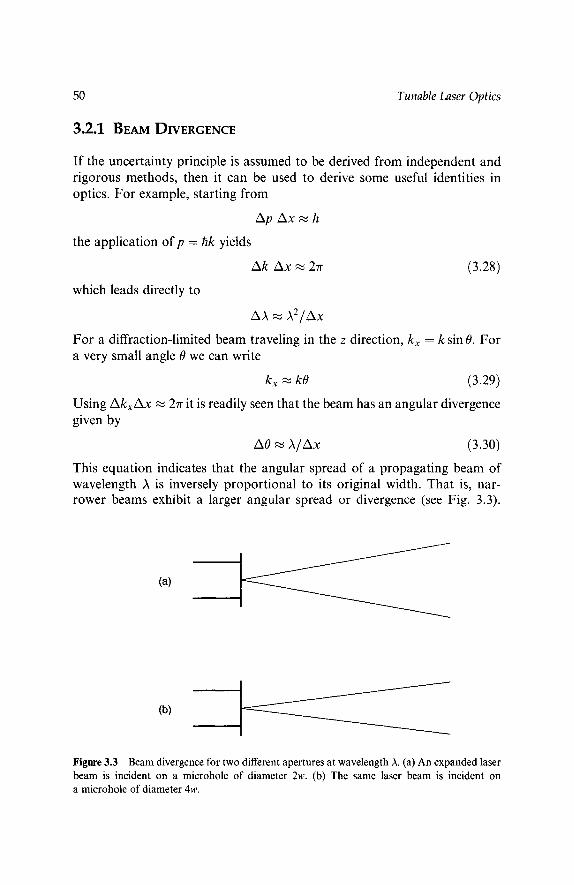
50 Tunable Laser Optics
3.2.1 BEAM DIVERGENCE
If the uncertainty principle is assumed to be derived from independent and rigorous methods, then it can be used to derive some useful identities in optics. For example, starting from
Ap A x ~ h
the application of p - hk yields
Ak Ax ~ 27r (3.28)
which leads directly to
AA ~ A 2 /Ax
For a diffraction-limited beam traveling in the z direction, kx = k sin 0. For a very small angle 0 we can write
kx ,.~ kO (3.29)
Using AkxAx ~ 27r it is readily seen that the beam has an angular divergence given by
AO ~ A /Ax (3.30)
This equation indicates that the angular spread of a propagating beam of wavelength A is inversely proportional to its original width. That is, nar- rower beams exhibit a larger angular spread or divergence (see Fig. 3.3).
(a) -----_.____
(b)
Figure 3.3 Beam divergence for two different apertures at wavelength A. (a) An expanded laser beam is incident on a microhole of diameter 2w. (b) The same laser beam is incident on a microhole of diameter 4w.
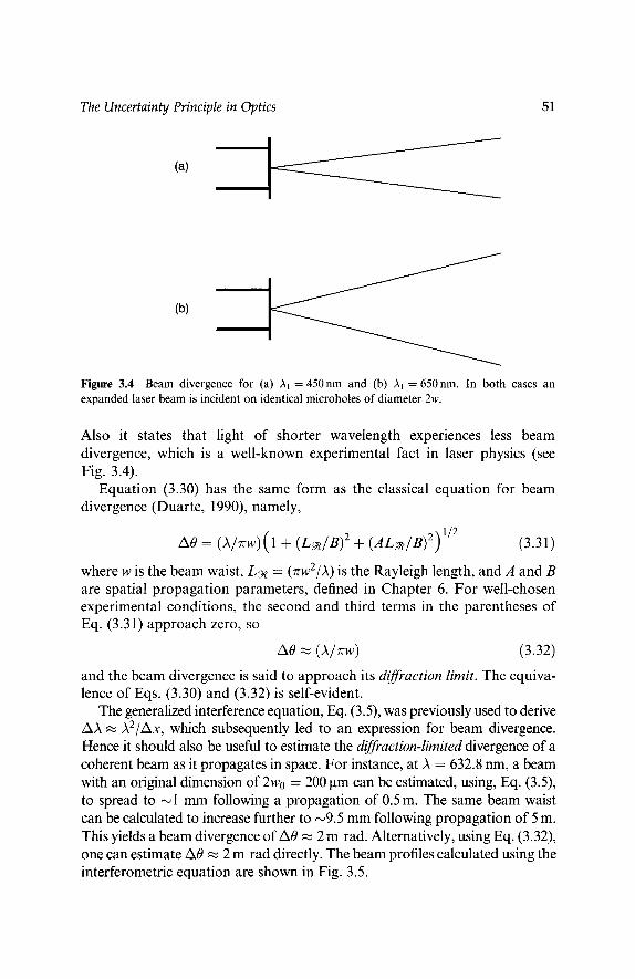
The Uncertainty Principle in Optics 51
(a)
(b)
Figure 3.4 Beam divergence for (a) Al = 450nm and (b) A1 = 650nm. In both cases an expanded laser beam is incident on identical microholes of diameter 2w.
Also it states that light of shorter wavelength experiences less beam divergence, which is a well-known experimental fact in laser physics (see Fig. 3.4).
Equation (3.30) has the same form as the classical equation for beam divergence (Duarte, 1990), namely,
A 0 - (A/Trw) (1 + (L~/B) 2 + (AL~/B)2) '/2 (3.31)
where w is the beam waist, L ~ = (Trw2/A) is the Rayleigh length, and A and B are spatial propagation parameters, defined in Chapter 6. For well-chosen experimental conditions, the second and third terms in the parentheses of Eq. (3.31) approach zero, so
AO ,.~ (A/Trw) (3.32)
and the beam divergence is said to approach its diffraction limit. The equiva- lence of Eqs. (3.30) and (3.32) is self-evident.
The generalized interference equation, Eq. (3.5), was previously used to derive AA ~ AZ/Ax, which subsequently led to an expression for beam divergence. Hence it should also be useful to estimate the diffraction-limited divergence of a coherent beam as it propagates in space. For instance, at A = 632.8 nm, a beam with an original dimension of 2w0 = 200 ~m can be estimated, using, Eq. (3.5), to spread to ~ 1 mm following a propagation of 0.5 m. The same beam waist can be calculated to increase further to ~9.5 mm following propagation of 5 m. This yields a beam divergence of A0 ~ 2 m rad. Alternatively, using Eq. (3.32), one can estimate A0 ~ 2 m rad directly. The beam profiles calculated using the interferometric equation are shown in Fig. 3.5.

52
(a)
40.0 -
-"~ 30.0 - t - t l ) ( . -
�9 g 20.0 - I1) rv
10.0 -
0.0 -4.0
Tunable Laser Optics
-2 .0 0.0 2.0 Screen Axial Distance (m)x 10 -3
4 .0
(b)
40.0 -
~ 3 0 . 0 - r
r B
(D
"~ 20.0 - m
rr"
10.0 -
0.0 -3.0 -2 .0 -1 .0 0.0 1.0 2.0
Screen Axial Distance (m) x 10 -2 3.0
Figure 3.5 Beam divergence determined from the generalized interference equation. (a) Beam profile following propagation through a distance of 0.5 m. (b) Beam profile following propagation through a distance of 5 m. Here, w0 = 100 gm and A = 632.8 nm. The divergence is determined by taking the difference at half width, half maximum and dividing by 4.5 m.
3 . 2 . 2 B E A M D I V E R G E N C E AND A S T R O N O M Y
C o n s i d e r p r o p a g a t i o n o f a d i f f r a c t i o n - l i m i t e d l ase r b e a m o v e r a d i s t a n c e o f
95 k m a t A - 589 n m fo r guide star a p p l i c a t i o n s in a s t r o n o m y . A m u l t i p l e -

53
(a)
prism-grating tunable laser oscillator (Duarte and Piper, 1984; Duarte, 1999) can be designed to provide single-longitudinal-mode oscillation at A- -589nm in a laser with a beam divergence that is nearly diffraction limited. Thus, its divergence is characterized by A0 ~ A/Trw. For a beam waist w ~ 125 lam, the corresponding beam divergence becomes A0 ..~ 1.5 m rad. If the beam of this oscillator were to be propagated over a distance of 95 km it would illuminate a circle nearly 285 m in diameter. This would yield a very weak power density. If, on the other hand, the beam is expanded, without introducing further divergence, by a factor of M ..~ 200, then the new beam divergence becomes A0 ~ A/MTrw. Now, as a consequence of the beam expansion, the beam diameter at the required propagation distance becomes about 1.42 m, which is close to the dimensions needed to achieve the necessary power densities with existing high-power tunable lasers. It should be mentioned that beam magnification factors of about 200 are not difficult to attain. Further, for this type of application the narrow-linewidth oscillator emission is augmented at amplifier stages, where the beam also increases its dimensions, thus reducing the requirements o n M .
One further application of the beam divergence equation relates to the angular resolution limit of telescopes used in astronomical observations. Reflection telescopes, such as the Newtonian and Cassegrain telescopes, are depicted in Fig. 3.6 and discussed further in Chapter 6. The angular resolution that can be accomplished with these telescopes under ideal con- ditions is approximately described by the diffraction limit given in Eq. (3.32).
The Uncertainty Principle in Optics
(b)
Figure 3.6 Reflection telescopes used in astronomical observations. (a) Newtonian telescope. (b) Cassegranian telescope.

54 Tunable Laser Optics
That is, the smallest angular discrimination, or resolution limit, of a tele- scope with a diameter D = 2w is given by
AO ~ 2A/TrD (3.33)
This equation indicates that the two avenues to increase the angular resolution of a telescope are either to observe at shorter wavelengths or to increase the diameter of the telescope. The latter option has been adopted by optical designers who have built very large telescopes. At A = 500 nm, the angular resolution for a telescope with D - 10 m is A0 ,~ 3.18 x 10 -8 rad. For an hypothetical diameter of D -- (1000/70 m the angular resolution at the same wavelength becomes A0 ~ 1.00 x 10 .9 rad. In addition to better angular resolutions, large aperture telescopes provide increased signal to noise ratios since the area of collection increases substantially. In the future, this class of telescope might be made available by advances in segmented optics technology.
3.2.3 THE UNCERTAINTY PRINCIPLE AND THE CAVITY LINEWIDTH EQUATION
As outlined by Duarte (1992), starting from
[(X[S)[ 2 -- ~ ~(rj) 2 if- 2 ~ q~(rj) m=j+l ffJ(rm) coS(am -- ~')j)
the equation for a diffraction grating, mA = 2d sin O, can be established. Considering two slightly different wavelengths, an expression for the wave- length difference can be written as
AA = (2d/m)(sin 01 - sin 02) (3.34)
For O1 ~ 02 (=0) this equation can be restated as
AA ~ (2d/m)AO(1 - ( 3 0 2 / 3 ! ) + (504/5!) . . . ) (3.35)
Differentiation of the grating equation leads to
(O0/OA) cos 19 = m/2d (3.36)
and substitution into Eq. (3.35) yields
/kA ~ A0(00/0A)-I (1 - (O2/2! ) -+- (O4/4! ) . . . ) / cos O (3.37)
which reduces to the well-known cavity linewidth equation (Duarte, 1992),

The Uncertainty Principle in Optics 55
m)k ~ mO(OO/O)k) -1 (3.38)
or
AA ~ A0(V~0) -~ (3.39)
where V~0 = (00/0A). This equation has been used extensively to determine the emission linewidth in pulsed narrow-linewidth dispersive laser oscilla- tors (Duarte, 1990). It originates in the generalized N-slit interference equation and incorporates AO, whose value can be determined either from the uncertainty principle or from the interferometric equation itself. This equation is well known in the field of classical spectrometers, where it was introduced using geometrical arguments (Robertson, 1955). In addition to its technical and computational usefulness, Eq. (3.38) and/or Eq. (3.39) illustrate the inherent interdependence between spectral and spatial coherence.
PROBLEMS
1. Calculate the diffraction-limited beam divergence at fullwidth, half max- imum (FWHM) for (a) a laser beam with a 100-gm radius at A = 590 nm, and (b) a laser beam with a 500-gm radius at A = 590 nm.
2. Repeat the calculations of the first problem for A = 308 nm. Comment. 3. Calculate the dispersive cavity linewidth for a high-power tunable laser
yielding a diffraction-limited beam divergence 100gm in radius, at A = 590nm. Assume that an appropriate beam expander illuminates a 3000-1/mm grating deployed in the first order. The grating has a 50-mm length perpendicular to the grooves.
4. (a) For a pulsed laser delivering a 350-MHz laser linewidth, estimate its shortest possible pulse width.
(b) For a laser emitting 10-fs pulses, estimate its broadest possible spec- tral width in nanometers centered around A = 600 nm.
5. Show that Eq. (3.29) can be expressed as Eq. (3.30).
REFERENCES
Dirac, P. A. M. (1978). The Principles of Quantum Mechanics, 4th ed. Oxford University Press, London.
Duarte, F. J. (1990). Narrow-linewidth pulsed dye laser oscillators. In Dye Laser Principles (Duarte, F. J., and Hillman, L. W., eds.). Academic Press, New York.
56 Tunable Laser Optics
Duarte, F. J. (1991). Dispersive dye lasers. In High-Power Dye Lasers (Duarte, F. J., ed.) Springer-Verlag, Berlin.
Duarte, F. J. (1992). Cavity dispersion equation AA ~ A0(00/0A)-I: a note on its origin. Appl. Opt. 31, 6979-6982.
Duarte, F. J. (1997). Interference, diffraction, and refraction, via Dirac's notation. Am. J. Phys. 65, 637-640.
Duarte, F. J. (1999). Multiple-prism grating solid-state dye laser oscillator: optimized architec- ture. Appl. Opt. 38, 6347-6349.
Duarte, F. J., and Piper, J. A. (1984). Narrow-linewidth, high-prf copper laser-pumped dye- laser oscillators. Appl. Opt. 23, 1391-1394.
Feynman, R. P., Leighton, R. B., and Sands, M. (1965). The Feynman Lectures on Physics, Vol. III. Addison-Wesley, Reading, MA.
Haken, H. (1981). Light. North Holland, Amsterdam. Robertson, J. K. (1955). Introduction to Optics: Geometrical and Physical. Van Nostrand, New
York.

Chapter 4
The Physics of Multiple-Prism Optics
4.1 INTRODUCTION
Multiple-prism arrays were first introduced by Newton (1704) in his book Opticks. In that visionary volume Newton reported on arrays of nearly isosceles prisms in additive and compensating configurations to control the propagation path and the dispersion of light. Further, he also illustrated slight beam expansion in a single isosceles prism. In his treatise, Newton does provide a written qualitative description of light dispersion in a sequence of prisms, thus laying the foundation for prismatic spectrometers and related instrumentation. In this chapter, a mathematical description of light dispersion in generalized multiple-prism arrays is given. Although the theory was originally developed to quantify the phenomenon of intracavity line- width narrowing, in multiple-prism-grating tunable laser oscillators (Duarte and Piper, 1982), it is applicable beyond the domain of tunable lasers to optics in general. The theory considers single-pass as well as multiple-pass dispersion in generalized multiple-prism arrays and is useful to both line- width narrowing and pulse compression. As a pedagogical tool, reduction of the generalized formulae to single-prism calculations are included in add- ition to a specific design of a particular practical high-magnification multiple- prism beam expander.
In order to facilitate the flow of information and to maintain the focus on the physics, some of the mathematical steps involved in the derivations are not included. For further details, references to the original work are cited.
57

58 Tunable Laser Optics
The mathematical notation is consistent with the notation used in the original literature.
4.2 GENERALIZED MULTIPLE-PRISM DISPERSION
Multiple-prism arrays are widely used in optics in a variety of applications, such as (a) intracavity beam expanders, in narrow-linewidth tunable laser oscillators, (b) extracavity beam expanders, (c) pulse compressors in ultrafast lasers, and (d) dispersive elements in spectrometers. Even though multiple-prism arrays were first introduced by Newton (1704), a mathemat- ical description of their dispersion had to wait a long time, until their application as intracavity beam expanders in narrow-linewidth tunable lasers (Duarte and Piper, 1982). Generalized multiple-prism arrays are depicted in Fig. 4.1. Considering the mth prism of the arrangements, the angular relations are given by
q~l,m -}- q~Z,m ~- Cm -}- Ogm
~)l,m q" ffdZ,rn = OLm
sin 4~l,m =nm sin ~l,m
sin ~2,m = n m sin ~2,m
(4.1)
(4.2)
(4.3)
(4.4)
As illustrated in Fig. (4.1), ~)l,m and ~)2,m are the angles of incidence and emergence, and ~l,m and ~2,m are the corresponding angles of refraction, at the mth prism. Differentiating Eqs. (4.3) and (4.4) and using
d~bl ,m / dn -- d~b2,m / dn (4.5)
the single-pass dispersion following the mth prism is given by (Duarte and Piper, 1982, 1983)
~7)~2,m -- O--~2,m~nm -t- (kl,mk2,m) -1 ( ~ l , m ~ ) ~ n m -Jr- ~7Aq~2,(m_l) ) (4.6)
where V~ = 0/0A and the following geometrical identities apply:
kl,m -- COS ~)l,m/COS q~l,m
k2,m = cos ~2 ,m/cos ff)2,m
~ l , m = tan q~l,m/nm ~ 2 , m = tan q~2,m/nm
(4.7)
(4.8)
(4.9)
(4.10)
The kl,m and k2,m factors represent the physical beam expansion experienced at the mth prism by the incidence and the emergence beams, respectively. The generalized single-pass dispersion equation indicates that the cumulative dispersion at the mth prism, namely, Va~z,m, is a function of the geometry of
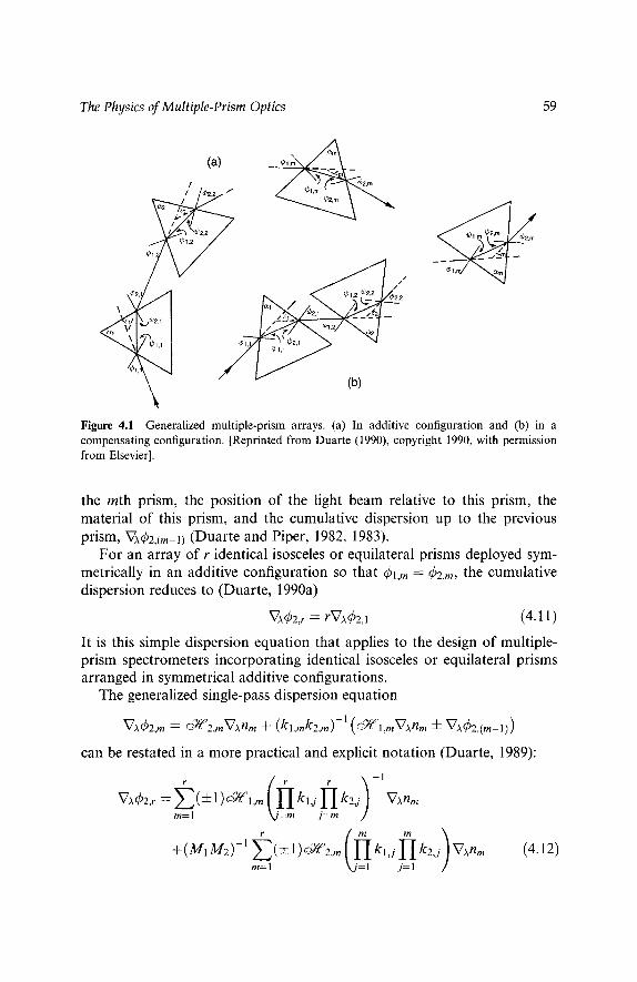
The Physics of Multiple-Prism Optics 59
/ (a) __~~/ , ") f~~,m
- - , / ' 1 , ~
7",e,,, ~ (b) .,,
Figure 4.1 Generalized multiple-prism arrays. (a) In additive configuration and (b) in a compensating configuration. [Reprinted from Duarte (1990), copyright 1990, with permission from Elsevier].
the mth prism, the position of the light beam relative to this prism, the material of this prism, and the cumulative dispersion up to the previous pr ism, ~7A~)Z,(m_l) (Duarte and Piper, 1982, 1983).
For an array of r identical isosceles or equilateral prisms deployed sym- metrically in an additive configuration so that r = (b2,m, the cumulative dispersion reduces to (Duarte, 1990a)
~7,~q52, r = r~7)~q52,1 ( 4 . 1 1 )
It is this simple dispersion equation that applies to the design of multiple- prism spectrometers incorporating identical isosceles or equilateral prisms arranged in symmetrical additive configurations.
The generalized single-pass dispersion equation
~7Ar m -- O_~2,m~7Anrn .-]- (kl,mk2,m) -1 (~ l , rn~TA/ ' /m q-- ~7Ar )
can be restated in a more practical and explicit notation (Duarte, 1989):
V)~ t~2,r = Z ( - ' I - 1) ~ ,~ l ,m klj k2r V~l"lm m= 1 =m "=
+(M1M2) -1 ( + l ) ~ 2 , m kl,j H k2,j V,Xrtrn m=l =1 j= l
(4.12)
60 Tunable Laser Optics
where
M1 - 1zI klj (4.13) j=l
M2 - ~ I k2j (4.14) j=l
are the respective beam expansion factors. For the important practical case of an array of r right angle prisms, designed for orthogonal beam exit (that is, q~2,m -- ~2,m -- 0), Eq. (4.12) reduces to
)' VA~b2,r- ~ (-+-l)~{~l,m klj ~7Anm (4.15)
m= 1 =m
If in addition the prisms have identical apex angles (OL1 = tY2 = Ol3 . . . . . tYm) and are configured to have the same angle of incidence (~bl,1 = ~bl,2 = ~bl,3 . . . . . ~bl,m), then Eq. (4.15) can be written as (Duarte, 1985)
VA~2,r- tan ~1,1 ~ (+l)(1/kl,m)m-lvAnm m=l
(4.16)
Further, if the angle of incidence for all prisms is Brewster's angle, then the single-pass dispersion reduces to the elegant expression
V~bZ,r - ~ (+l)(1/nm)mV~,nm (4.17) m-1
4.2.1 DOUBLE-PASS GENERALIZED MULTIPLE-PRISM DISPERSION
The evaluation of intracavity dispersion in tunable laser oscillators incor- porating multiple-prism beam expanders requires the assessment of the double-pass, or return-pass, dispersion. The double-pass dispersion of multi- ple-prism beam expanders was derived by thinking of the return pass as a mirror image of the first light passage, as illustrated in Fig. 4.2. The return- pass dispersion corresponds to the dispersion experienced by the return light

The Physics of Multiple-Prism Optics 61
Symmetric half
I ! I ]
I el, Grating ~'~'~r-1
or Mirror
~1'1/~. k ? I,~2r Figure 4.2 Multiple-prism beam expander geometry in additive configuration and its mirror image. A dispersive analysis through the multiple-prism array and its mirror image is equivalent to a double-pass, or return-pass, analysis. [Reprinted from Duarte and Piper (1982), copyright 1982, with permission from Elsevier].
beam at the first prism. Thus, it is given by O~tl,m/O)~- ~A~ t where the 1,m~ prime character indicates return pass (Duarte and Piper, 1982, 1984):
~7A~l,m __ O_~tl,m~7~llm_.l..(kt 1 , - 1 ( t ) t ,mk2,m ) ~ 2 , m ~ A ? l m _4_ ~7Aq~tl,(m+l) (4.18)
where
kll m ! ! ,m COS ffOl,m/COS ~l,m
k~2,m -- COS r ,//)t 2,m ~ l , m -- tan r 1 ,m//'/m
o_~2, m - tan r 2,m/nm
(4.19)
(4.20)
(4.21)
(4.22)
Here, ~7lq~],(m+l ) provides the cumulative single-pass multiple-prism disper- sion plus the dispersion of the diffraction grating; that is,
= + V r (4.23)
where VaOa is the grating dispersion. If the grating is replaced by a mirror, then we simply have the prismatic contribution and
VaqStl,(m+l) = Va~bZ,r (4.24)
Defining ~7Aq~], m --~7(I)p, where the capital phi stands for return pass and P stands for for multiple prism, the explicit version of the generalized

62 Tunable Laser Optics
double-pass dispersion for a multiple-prism mirror system is given by (Duarte, 1985, 1989)
-1 VA~p =2M1 M2 (-+- l ) ~al,m klj k2j
m=l =m "=
+ 2 ( - + - l ) ~ 2 , m kid Hk2d VAnm m=l =1 j = l
V~nm
(4.25)
For the case of r right angle prisms, designed for orthogonal beam exit (that is, q~2,m - ~b2,m -- 0), Eq. (4.25) reduces to
r C " ) VAmp -- 2M1 ~(+l)~_Tfl,m klj
m=l =m
-1
~7A/"/m (4.26)
which can also be expressed as (Duarte, 1985)
gTA~p- 2~m=l (+ 1)(j]~ k l j )= l tan~bl,mV:~nm (4.27)
If the angle of incidence for all prisms in the array is made equal to the Brewster angle, this equation simplifies further to (Duarte, 1990a)
V~,~bF, - 2 ~ (-'}-l )(nm)m-l~7Anm (4.28) m=l
4.2.2 MULTIPLE RETURN-PAss GENERALIZED MULTIPLE-PRISM DISPERSION
Here we consider a multiple-prism grating or multiple-prism mirror assem- bly, as illustrated in Fig. 4.3. The light beam enters the first prism of the array; it is then expanded and either diffracted back or reflected back into the multiple-prism array. In a dispersive laser oscillator this process goes forth and back many times, thus giving rise to the concept of intracavity double pass, or intracavity return pass. For the first return pass, toward the first prism in the array, the dispersion is given by Eq. (4.18). If N denotes the

The Physics of Multiple-Prism Optics 63
Figure 4.3 Multiple-prism grating assembly used to perform a dispersive multiple-return-pass analysis. [Reprinted from Duarte and Piper (1982), copyright 1982, with permission from Elsevier].
number of passes toward the grating or the reflecting element and 2N denotes the number of return passes toward the first prism in the sequence, we have
(VA~)Z,m)N -- Q-~2,mVArtm -[-(kl,mkz,m) -1 (~l,mVArtm -+- (VA~Z,(m-1))N) (4.29)
' ' ' - l ( ' ' N) (V,X~I,m)2N -- ~l,mV~nm + (k~l,mk2,m) ~2,mV,xnm -Jr- (~7~l,(m+l)) 2 (4.30)
For the first prism of the array, (Va~b2,(m-1))u (with N = 3, 5, 7 , . . . ) in Eq. (4.29) is replaced by (VaqS'l,1)2u (with N - 1, 2, 3, . . .) . Likewise for the last prism of the assembly, (VaqS'l,(m+l))ZU (with N - 1, 2, 3 , . . . ) in Eq. (4.30) is replaced by (VaOa + (Vaq52,r)u) (with N = 1, 3, 5,. . .) . In the case where the grating is replaced by a mirror, this expression becomes simply (Vaq52,r)U (with N = 1, 3, 5, . . .) . Thus, the multiple return-pass dispersion for a multi- ple-prism grating assembly is given by (Duarte and Piper, 1984)
(V:~0)R = (RMV~,Oa + R V ~ p ) (4.31)
where R is the number of return passes. This equation illustrates the very important fact that in the return-pass dispersion of a multiple-prism grating assembly, the dispersion of a grating is multiplied by the factor RM, where M is the overall beam magnification of the multiple-prism beam expander. Once again, if the grating is replaced by a mirror, that is, X7~OG = 0, the dispersion reduces to
(V~0)R = RX7A~e (4.32)
which implies that the multiple-prism intracavity dispersion increases linearly as a function of R.

64 Tunable Laser Optics
4.2.3 SINGLE-PRISM EQUATIONS
Using Eq. (4.6) for m = 1 yields
V~c/)2,1- ~d~Z,lV~nl + (kl,lkz,1)-l(~l,lV:~nl) (4.33)
which can also be expressed as
V~2,1 -- ((sin ~P2,1/cos 4~2,1) + (cos ~2,1/cos q52,1) tan ~Pl,~) V~n (4.34)
Division by V~n yields the result given for V, qS2,1 by Born and Wolf (1999). For orthogonal beam exit (q52,1 ,-~ ~P2,1 ~ 0) Eq. (4.34) simplifies to
~7Aq~2,1 ~ tan ~31,1V~n (4.35)
which is the result given by Wyatt (1978). For a single prism designed for orthogonal beam exit and deployed at
Brewster's angle of incidence, Eq. (4.17) becomes
~7A ~)2,1 = (1 In) V:~n (4.36)
a result that also follows from Eq. (4.35). For a double-pass analysis, for m = 1, Eq. (4.18), becomes
' YAH1--~-(k' l k ' ) - I ( Q _ ~ , VAg/I-I-VA~2,1) v~r 1 ~ ~-{~1,1 ,1 2,1 2,1 (4.37)
which for orthogonal beam exit reduces to
Vamp = 2(k1,1 t an ~)I,1)VAn (4.38)
For incidence at the Brewster angle this equation simplifies to
V ~ p = 2V~n (4.39)
Reduction from Eq. (4.38) to Eq. (4.39) implies that at the Brewster angle of incidence the beam magnification
kl,1 = n (4.40)
tan ~Pl,1 = (1/n) (4.41)
4.3 MULTIPLE-PRISM DISPERSION A N D LINEWIDTH N A R R O W I N G
In Chapter 3, the cavity linewidth equation was derived from interferometric principles as (Duarte, 1992)
z ~ - A0(V~0) -1 (4.42)

The Physics of Multiple-Prism Optics 65
where A0 is the beam divergence and V~0 is the overall intracavity disper- sion. The message from this equation is that for narrow-linewidth emission we need to minimize the beam divergence and to increase the intracavity dispersion. The multiple return-pass cavity linewidth for dispersive oscillator configurations, as illustrated in Fig. 4.4, is given by (Duarte, 200 l a)
zSA - AOR(MRVaOa + R~7A(I)p) -1 (4.43)
and the multiple return-pass beam divergence (see Chapter 6) is given by
AOR - - (A/Tl'w) (1 q-(L,~/BR) 2 + (ARL~/BR) 2) 1/2 (4.44)
Here, AR and BR are multiple-pass propagation matrix coefficients and L ~ = 7rwZ/A (where w is the beam waist) is known as the Rayleigh length. For an optimized multiple-prism grating laser oscillator, A0R approaches its diffraction limit following a few return passes.
4.3.1 THE MECHANICS OF LINEWIDTH NARROWING IN OPTICALLY PUMPED PULSED LASER OSCILLATORS
The factor R in the multiple-return-pass linewidth equation is related to the total intracavity transit time from the beginning of the excitation pulse to the onset of laser oscillation. Thus, R is determined experimentally by measuring the time delay &- between the leading edge of the pump pulse and the leading edge of the laser emission pulse. This perspective is consistent with the mechanics of recording single-pulse interferograms, which provide a laser linewidth at the early stages of oscillation that is broader than at subsequent times of emission. That is, although the linewidth narrowing continues throughout the duration of the laser emission, the time-integrated recording process (using photographic means, for instance) yields information as broad as that recorded at the onset of the laser oscillation. Once &- has been measured, the number of return intracavity passes is given by
R = &-/At (4.45)
where At is the time taken by the emission to cover twice the cavity length (At = 2L/c), so
R = &-(c/2L) (4.46)
In summary, from the beginning of the pulsed laser excitation the R factor contributes to reduce both the beam divergence and the laser linewidth. As indicated by Eq. (4.44) the beam divergence can decrease only toward its

66 Tunable Laser Optics
Figure 4.4 (a) MPL grating laser oscillator incorporating a (+, + , + , - ) multiple-prism con- figuration and (b) a ( + , - , + , - ) multiple-prism configuration. (c) HMPGI grating laser oscil- lator incorporating a compensating double-prism configuration. In this oscillator, the refraction angle identified as 0' corresponds to ft. [Reprinted from Duarte (1995c), copyright 1995, with permission from Elsevier].
The Physics of Multiple-Prism Optics 67
diffraction limit, while the laser linewidth decreases linearly as a function of R. In turn, R is a finite number that can be as low as R ~ 3 for high-power short-pulse excitation. It is also necessary to remember that Eq. (4.43) is the dispersive cavity linewidth equation; that is, it quantifies the ability of a dispersive oscillator cavity to narrow the frequency transmission window of the cavity. Once the dispersion linewidth limits emission to a single long- itudimal mode, the actual linewidth of that mode is determined by the dynamics of the laser. For further information on this subject the reader should refer to Duarte and Piper (1984) and Duarte (2001a).
4.3.2 DESIGN OF ZERO-DISPERSION MULTIPLE-PRISM BEAM EXPANDERS
In practice, the dispersion of the grating multiplied by the beam expansion, that is, M(V~O6), amply dominates the overall intracavity dispersion. Thus, it is desirable to remove the dispersion component originating from the multiple-prism beam expander so that
z2~ ~ AOR(MRV~OG) -1 (4.47)
In such designs the tuning characteristics of the laser are those of the grating around a specific wavelength. To illustrate the design of a quasi-achromatic multiple-prism beam expander, a case of practical interest, with M ,~ 100 and a four-prism expander deployed in a compensating configuration similar to that outlined in Fig. 4.4, is considered. The compensating configuration selected is (+, +, + , - ) ; that is, the additive dispersion of the first three prisms is subtracted by the fourth prism, thus yielding zero overall disper- sion. Multiple-prism beam expanders deployed intracavity in tunable lasers employ right angle prisms designed for orthogonal beam exit; that is ~2,m ~ ~2,m ~ 0. Thus, we must have Va~p = 0 in Eq. (4.27) so that (Duarte, 1985)
(kl,1 + kl,lkl,2 q- kl,lkl,2kl,3) tan ~1,1 -- (kl,lkl,2kl,3)kl,4 tan r (4.48)
where
t a n ~31,1 ~ tan ~1,2 = t a n ~1,3 (4.49)
A particular wavelength of interest in tunable lasers is A = 590 nm. At this wavelenth, for a material such as optical crown glass, n - 1.5167. For M ~ 100 we select
kl,1 -- kl,2 = kl,3 -- 4

68 Tunable Laser Optics
This means that for the first three prisms,
~1,1 = q)l ,2 ~--- q~l,3 = 79.01~ and 1/)1,1 - - @1,2 • @1,3 - - 40.330
which also becomes the apex angle of the first three prisms. Using Eq. (4.48) it is found that for the fourth prism, 4~1,4 = 59.39 ~ @1,4 = 34.57 ~ and k l , 4 - - 1 . 6 2 . This yields an overall beam magnification factor of M = 103.48. Normally the beam waist w in a well-designed high-power multiple-prism grating laser oscillator is about 100 gm. This means that the expanded beam at the exit surface of the fourth prism is 2 w M ~ 20.7 mm. Thus, this particular multiple-prism beam expander can comprise three small prisms with a hypotenuse of 17 mm, though the first two can be even smaller. The larger, fourth prism requires a hypotenuse of 27 mm. The thickness of all prisms can be 10 mm. The surface of these prisms are usually polished to yield a surface flatness of A/4 or better.
The design of compact solid-state multiple-prism laser oscillators, as illustrated in Fig. 4.4, requires the use of small prism beam expanders with M ~ 40. The exercise is now repeated for r = 2 in Eq. (4.27). Setting V ~ p = 0 we obtain (Duarte, 2000)
tan @1,1 = kl,2 t a n / / ; 1 , 2 (4.50)
For k l , 1 --- 30, ~1,1 ~--- 88.560 and ~)1,1 = 41.23 ~ Hence, for the second prism, Eq. (4.50) yields q51,2 = 53.05 ~ ~1,2 = 31.80 ~ and kl,2 = 1.41. Therefore, the overall intracavity beam expansion becomes k l , lk l ,2 = 42.41. For a beam waist of w = 100 gm this implies 2 w M ,.~ 8.48 mm. These dimensions require the first prism to have a hypotenuse of ~8 mm and the second prism a hypotenuse of ~ 10 mm.
4.4 MULTIPLE-PRISM DISPERSION A N D PULSE COMPRESSION
Prismatic pulse compression was demonstrated for the first time by Dietel etal. (1983), yielding a pulse duration of 53 fs. A prism compensating pair was introduced by Diels etal. (1985), obtaining a pulse duration of 85 fs. Two compensating prism pairs as pulse compressors were demonstrated by Fork etal. (1984), who reported pulses of 65 fs. Generalized dispersion equations applicable to pulse compression were introduced by Duarte and Piper (1982) and Duarte (1987). Various pulse compression configurations are depicted in Fig. 4.5.
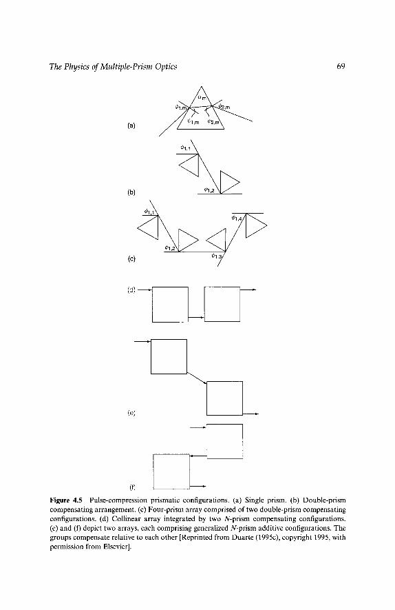
The Physics of Multiple-Prism Optics
(a)
(b)
(c)
69
(d)
(e)
(f) Figure 4.5 Pulse-compression prismatic configurations. (a) Single prism. (b) Double-prism compensating arrangement. (c) Four-prism array comprised of two double-prism compensating configurations. (d) Collinear array integrated by two N-prism compensating configurations. (e) and (f) depict two arrays, each comprising generalized N-prism additive configurations. The groups compensate relative to each other [Reprinted from Duarte (1995c), copyright 1995, with permission from Elsevier].

70 Tunable Laser Optics
In the laser linewidth equation
= x0(v 0)
~7~0 is the overall intracavity dispersion. In laser cavities designed for narrow-linewidth oscillation, ~7~0 is very large and is dominated by the dis- persion of the grating, which is often multiplied by M. By contrast, in the case of ultrashort-pulse lasers, as a consequence of the uncertainty principle (see Chapter 3), the emission spectrum is broadband, which is associated with a small value for ~7~0.
As discussed by Diels (1990), the phase factor in a femtosecond laser pulse depends on the addition of ~72n and ~72p terms. Here, P is the optical path length of the compressor, whose derivative with respect to wavelength is given by
~7~e = ~,~nVnC~VO P (4.51)
and its second derivative is (Fork et al., 1984)
~72p - (~72n~Tn~5 + (~TAn)2V2nq~) ~Tq~P -~-(~7An)2(VnqS)2~7~P (4.52)
where ~7~n is the prism material dispersion, 272- 02/0~ 2, ~72n is the derivative of the prism material dispersion, ~'~P is the angular derivative of the path length, and V~P is the second angular derivative of the path length. In general, ~7~n is a negative number and 272n is a positive number and
IV2nl >> IV nl (4.53)
Numerical values for n, ~7~n, and 272n for some well-known materials are given in Table 4.1.
In order to compress ultrashort pulses with a large positive chirp, gTZp should be a large negative number (Diels, 1990). From Eqs. (4.6), (4.18), and (4.25) it should be evident that the prismatic dispersion can be made positive or negative at will by choice of design and configuration. For a generalized multiple-prism array ~7n~ and ~72~b correspond to ~n~Z,m and ~72q~Z,m, respectively. The first derivative can be obtained by using the identity
Vn~2,m -- Vk(P2,rn(~TAnm) -1 (4.54)

The Physics of Multiple-Prism Optics 71
Table 4.1 Dispersion Characteristics of Prism Materials for Pulse Compression
Material n A V~n V 2n (lam) (btm-') (lam -2)
Reference
Quartz 1.457 0.62 -0.03059 0.1267 BK7 1.51554 0.62 -0.03613 0.15509 F2 1.61747 0.62 -0.07357 0.34332 SF 10 1.72444 0.62 -0.10873 0.53819 LaSF9 1.84629 0.62 -0.11189 0.57778
1.83257 0.80 -0.05201 0.18023 ZnSe a 2.586 0.62 -0.698 5.068
2.511 0.80 -0.246 1.163
Fork etal. (1984)
Diels (1990) Diels (1990)
Source: Duarte, 1995b. a Calculated using data from Marple, 1964.
and the second derivative is given by Duarte (1987)
2 Vn~2,m --~-ga2,m(VnO2,m)2nm + (kl,mk2,m) -!
X {(~--~l,mXl,mkl,mVnr -1- V2nq52,(m-1)) -~- (~gal ,m -]- Vnq52(m-1))
(Xl,mVn~31,m -- ~2,mk2,mVn~32,m - ~l,mkl,mVn~l,mnm) }
-~-(k2,m) -1 (Vnr + Vnr (4.55)
where
Xl,m = tan ~l,m (4.56)
For a single isosceles prism, that is, m - 1, deployed for minimum deviation and Brewster's angle of incidence, Eqs. (2.54) and (2.55) reduce to
Vnq52,1 -- 2 (4 .57)
V2q52,1 -- (4n- ( 2 / n 3 ) ) (4.58)
which are the single-prism results given by Fork et al. (1984). Using P = 2l cos r Duarte (1987) calculated (at A = 620 nm) the required prism separation length to achieve negative dispersion for an isosceles prism sequence, as illustrated in Fig. 4.5c, for prisms made of quartz, LaSF9, and ZnSe. Those calculations

72 Tunable Laser Optics
demonstrated a significant reduction in the required prism separation as the index of refraction of the prism material increased. For a single-prism material, the required prism separation decreases as the angle of incidence increases until a minimum is reached. A rapid increase is observed following the minimum. The effect of minute angular deviations from the Brewster angle of incidence on ~n~PZ,m and ~72052,m was quantified by Duarte (1990b). A detailed discussion of pulse compression can be found in Diels and Rudolph (1996).
4.5 APPLICATIONS OF MULTIPLE-PRISM ARRAYS
So far, the use of multiple-prism arrays as intracavity beam expanders in narrow-linewidth tunable laser oscillators and as pulse compressors in ultrafast lasers has been examined. However, multiple-prism arrays as one- dimensional telescopes have found a variety of alternative applications as follows.
Extracavity double-prism beam expander to correct the ellipticity of laser beams generated by semiconductor lasers (Maker and Ferguson, 1989). These expanders make use of the prism pairs first introduced by Brewster (1813). Generalized laser beam shaping devises as discussed by Duarte (1995c). Beam-expanding devices for optical computing (Lohmann and Stork, 1989) One-dimensional beam expanders yielding extremely elongated Gaussian beams, with minimum height to width with ratios of 1:1000, for scanning applications (Duarte, 1987, 1993, 1995a). This includes characterization of transmission and reflection imaging surfaces. Multiple-prism beam expansion for N-slit interferometry (Duarte, 1991, 1993). One-dimensional multiple-prism telescopes in conjunction with digital detectors (Duarte, 1993, 1995a). This includes applications in conjunction with transmission grating in areas of wavelength measurements (Duarte, 1995c) and secure optical communications (Duarte, 2002). One-dimensional beam expansion for application in laser exposing devices known as laser sensitometers (Duarte, 2001 b).
PROBLEMS
1. Show that Eq. (4.6) can also be expressed in its explicit form of Eq. (4.12). 2. Show that for orthogonal beam exit, Eq. (4.12) reduces to Eq. (4.15). 3. Show that for prisms with (c~1 = c~2 = c~3 . . . . . C~m) and deployed for
Brewster's angle of incidence, Eq. (4.15) can be restated as Eq. (4.17).

The Physics of Multiple-Prism Optics 73
4. D e s i g n a t h r e e - p r i s m b e a m e x p a n d e r w i th Vaq~e = 0 for M ~ 70. A s s u m e
A = 590 n m , n = 1.5167 a n d w = 100 lam.
5. S h o w t h a t for m = 1, o r t h o g o n a l b e a m exit , a n d B r e w s t e r ' s ang le o f
inc idence , Eq. (4.18) r educes to Eq. (4.39).
REFERENCES
Born, M., and Wolf, E. (1999). Principles of Optics, 7th ed. Cambridge University Press, Cambridge, UK.
Brewster, D. (1813). A Treatise on New Philosophical Instruments for Various Purposes in the Arts and Sciences with Experiments on Light and Colours. Murray and Blackwood, Edinburgh.
Diels, J.-C. (1990). Femtosecond dye lasers. In Dye Laser Principles (Duarte, F. J. and Hillman, L. W., ed.). Academic, New York, pp. 41-132.
Diels, J.-C., and Rudolph, W. (1996). Ultrafast Laser Pulse Phenomena. Academic Press, New York.
Diels, J.-C., Dietel, W., Fontaine, J. J., Rudolph, W., and Wilhelmi, B. (1985). Analysis of a mode-locked ring laser: chirped-solitary-pulse solutions. J. Opt. Soc. Am. B, 2, 680-686.
Dietel, W., Fontaine, J. J., and Diels, J.-C. (1983). Intracavity pulse compression with glass: a new method of generating pulses shorter than 60 fs. Opt. Lett. 8, 4-6.
Duarte, F. J. (1985). Note on achromatic multiple-prism beam expanders. Opt. Commun. 53, 259-262.
Duarte, F. J. (1987). Generalized multiple-prism dispersion theory for pulse compression in ultrafast dye lasers. Opt Quantum Electron. 19, 223-229.
Duarte, F. J. (1989). Transmission efficiency in achromatic nonorthogonal multiple-prism laser beam expanders. Opt. Commun. 71, 1-5.
Duarte, F. J. (1990a). Narrow-linewidth pulsed dye laser oscillators. In Dye Laser Principles (Duarte, F. J. and Hillman, L. W., eds.). Academic Press, New York, pp. 133-183.
Duarte, F. J. (1990b). Prismatic pulse compression: beam deviations and geometrical pertur- bations. Opt. Quantum Electron. 22, 467-471.
Duarte, F. J. (1991). Dispersive dye lasers. In High-Power Dye Lasers (Duarte, F. J., ed.). Springer-Verlag, Berlin, pp. 7-43.
Duarte, F. J. (1992). Cavity dispersion equation ~ ~ &0(00/0A)-l: a note on its origin. Appl. Opt. 31, 6979-6982.
Duarte, F. J. (1993). On a generalized interference equation and interferometric measurements. Opt. Commun. 103, 8-14.
Duarte, F. J. (1995a). Interferometric imaging. In Tunable Laser Applications (Duarte, F. J., ed.). Marcel Dekker, New York, pp. 153-178.
Duarte, F. J. (1995b). Dye lasers. In Tunable Lasers Handbook (Duarte, F. J., ed.). Academic Press, New York, pp. 167-218.
Duarte, F. J. (1995c). Narrow-linewidth laser oscillators. In Tunable Lasers Handbook (Duarte, F. J., ed.). Academic Press, New York, pp. 9-32.
Duarte, F. J. (2000). Multiple-prism arrays in laser optics. Am. J. Phys. 68, 162-166. Duarte, F. J. (200 l a). Multiple-return-pass beam divergence and the linewidth equation. Appl.
Opt. 40, 3038-3041. Duarte, F. J. (2001 b). Laser sensitometer using multiple-prism beam expansion and a Polarizer.
US Patent No. 6236461.

74 Tunable Laser Optics
Duarte, F. J. (2002). Secure interferometric communications in free space. Opt. Commun. 205, 313-319.
Duarte, F. J., and Piper, J. A. (1982). Dispersion theory of multiple-prism beam expander for pulsed dye lasers. Opt. Commun. 43, 303-307.
Duarte, F. J., and Piper, J. A. (1983). Generalized prism dispersion theory. Am. J. Phys. 51, 1132-1134.
Duarte, F. J., and Piper, J. A. (1984a). Narrow-llinewidth; high prf copper laser-pumped dye laser oscillators. Appl. Opt. 23, 1391-1394.
Duarte, F. J., and Piper, J. A. (1984b). Multi-pass dispersion theory of prismatic pulsed dye lasers. Optica Acta 31, 331-335.
Fork, R. L., Martinez, O. M., and Gordon, J. P. (1984). Negative dispersion using pairs of prisms. Opt. Lett. 9, 150-152.
Lohmann, A. W., and Stork, W. (1989). Modified Brewster telescopes. Appl. Opt. 28, 1318- 1319.
Maker, G. T., and Ferguson, A. I. (1989). Frequency-modulation mode locking of a diode- pumped Nd:YAG laser. Opt. Lett. 14, 788-790.
Marple, D. T. F. (1964). Refractive index of ZnSe, ZnTe, and CdTe. J. Appl. Phys. 35, 539-542. Newton, I. (1704). Opticks. Royal Society, London. Wyatt, R. (1978). Comment on "On the dispersion of a prism used as a beam expander in a
nitrogen laser." Opt. Commun. 26, 9-11.

Chapter 5
Linear Polarization
5.1 MAXWELL EQUATIONS
Maxwell equations are of fundamental importance since they describe the whole of classical electromagnetic phenomena. From a classical perspective, light can be described as waves of electromagnetic radiation. As such, Maxwell equations are very useful to illustrate a number of the character- istics of light including polarization. It is customary just to state these equations without derivation. Since our goal is simply to apply them, the usual approach will be followed. However, for those interested, a derivation by Dyson (1990), attributed to Feynman, is available in the literature. Maxwe l l equations in the rationalized metric system are given by
v . s = 0 (5.1)
V . E = p/co (5.2)
c2V • a = oE/ot +j/~o (5.3)
~7 >< E = - O B / O t (5.4)
(Feynman et al., 1965). These equations illustrate, with succinct beauty, the unique coexistence in nature of the electric field and the magnetic field. The first two equations give the value of the given flux through a closed surface, and the second two equations give the value of a line integral around a loop. In this notation,
v = (OlOx, OlOy, O l & )
75

76 Tunable Laser Optics
E is the electric vector, B is the magnetic induction, p is the electric charge density, j is the electric current density, co is the permittivity offree space, and c is the speed of light. In addition to Maxwell equations, the following identities are useful:
j - erE (5.5)
D = eE (5.6)
B = # H (5.7)
Here, D is the electric displacement, H is the magnetic vector, er is the specific conductivity, e is the dielectric constant (or permittivity), and # is the magnetic permeability.
In the Gaussian systems of units, Maxwell equations are given in the form of
v . B = o (5.8) V. E = 4rrp (5.9)
V x H = (1/c)(OD/Ot + 4rrj) (5.10)
V • E = - ( 1 / c ) ( O B / O t ) (5.11)
(Born and Wolf, 1999). It should be noted that many authors in the field of optics prefer to use Maxwell equations in the Gaussian system of units. As explained by Born and Wolf (1999), E, D, j, and p in this system are measured in electrostatic units, and H and B are measured in electromag- netic units. The use of Maxwell equations in this book is consistent with the tradition established by Born and Wolf.
For the case of no charges or currents, that is, j - 0 and p - 0, and a homogeneous medium, Maxwell equations and the given identities can be applied in conjunction with the vector identity
V x V • E = VV. E - ~72E (5.12)
to obtain wave equations of the form (Born and Wolf, 1999)
V2F - ( l 2)(02F lOt 2) - 0 (S.13)
This leads to an expression for the velocity of propagation
1~ = C I ( C ~ ) 1/2 (5.14)
Comparison of this expression with the law of refraction, derived in Chapter 2, leads to what is known as Maxwell's formula (Born and Wolf, 1999):
(S.lS)

Linear Polarization 77
Here, n is the refractive index. It is useful to note that in vacuum
r __~_ l/C0#0 (5.16)
in the rationalized metric system, where #0 is the permeability of free space (Lorrain and Corson, 1970).
5.2 POLARIZATION A N D REFLECTION
Following the convention of Born and Wolf (1999), we consider a reflection boundary, depicted in Fig. 5.1, and a plane of incidence established by the incidence ray and the normal to the reflection surface. Here, the reflected component ~ll is parallel to the plane of incidence, and the reflected com- ponent ~ x is perpendicular to the plane of incidence.
For the case of #l = # 2 = l , Born and Wolf (1999) consider the electric and magnetic vectors as complex plane waves. In this approach, the incident electric vector is represented by equations of the form
E(x i) - _All cos dp(e-in )
E(i) _ _Ax(e-i~i)
g ~ i) - - -All sin ~(e -in)
(5.17)
(5.18)
(5.19)
where All and A• are complex amplitudes and Ti is the usual plane-wave phase factor, written as Ti = ~ [t - (x sin ~b + z cos cb)/v]. Using corresponding
I RII
~"--~ I _ . ~ R l
T•
Figure 5.1 Reflection boundary defining the plane of incidence.

78 Tunable Laser Optics
equations for E and H for transmission and reflection in conjunction with Maxwell's relation, with # = 1, and the law or refraction, Born and Wolf (1999) derive the Fresnelformulae:
Q_UII = ((2 sin ~bcos qS)/sin(q5 + ~b) cos(q5 - ~b))Aii
~ • = ((2 sin ~bcos qS)/sin(q5 + ~b))A•
~11 = (tan(q5 - ~b)/tan(q5 + ~b))Aii
~ • = (sin(q~ - ~b)/sin(~5 + ~b))A•
(5.20)
(5.21)
(5.22)
(5.23)
Using these equations the transmissivity and reflectivity can be expressed as
d-tl - ((sin 2q5 sin 2~b)/sin2(q5 + ~b) cos2(~b - ~b))
~ z - ((sin 2~b sin 2~b)/sin2(~b + ~b))
~ll -- (tan2( q5 - ~b)/tan2(q5 + @))
~ z - (sin2(q5 - ~b)/sin2(q5 + ~b))
(5.24)
(5.25)
(5.26)
(5.27)
and
~11 + ~--~11 = 1 (5.28) ~ • + ~ • = 1 (5.29)
Using these expressions for transmissivity and reflectivity, the degree of polarization, ~ , is defined as (Born and Wolf, 1999)
+ (s.30)
The usefulness of these equations is self-evident once ~ll is calculated as a function of angle of incidence (Fig. 5.2) for fused silica at 594nm (n = 1.4582). Here we see that ~11 = 0 at 55.5586 degrees. At this angle (4~ + 9) becomes 90 degrees so that tan (~b + 9) approaches infinity thus causing ~11 = 0. This particular ~b, known as the Brewster angle (~@), has a very important role in laser optics. Since at 4~ = 4~ the angle of refraction becomes 9 - (90 - ~b) ~ the law of refraction takes the form of
tan q~ = n (5.31)
For orthogonal, or normal, incidence, the difference between the two polariza- tions vanishes. Using the law of refraction and the appropriate trigonometric identities in Eqs. (5.24)-(5.27), it can be shown that (Born and Wolf, 1999)
- ( ( n - 1)/(n + 1)) 2 (5.32)
~_U - (4n/(n + 1)) 2 (5.33)
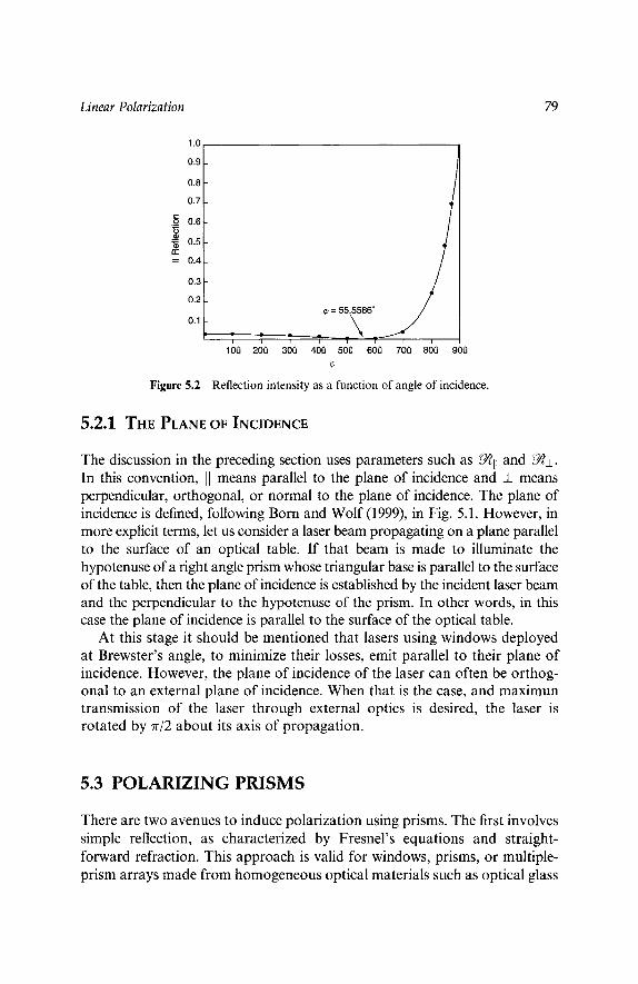
Linear Polarization 79
1.0
0.9
0 .8 -
0.7-
.~ 0 . 6 -
o.5- rr -- 0.4-
0.3-
0.2- q~ = 55.5586 ~
i i i I ] i i i
100 200 30s 400 500 600 700 800 )00
Figure 5.2 Reflection intensity as a function of angle of incidence.
5.2.1 THE PLANE OF INCIDENCE
The discussion in the preceding section uses parameters such as ~1t and ~• In this convention, 1] means parallel to the plane of incidence and • means perpendicular, orthogonal, or normal to the plane of incidence. The plane of incidence is defined, following Born and Wolf (1999), in Fig. 5.1. However, in more explicit terms, let us consider a laser beam propagating on a plane parallel to the surface of an optical table. If that beam is made to illuminate the hypotenuse of a fight angle prism whose triangular base is parallel to the surface of the table, then the plane of incidence is established by the incident laser beam and the perpendicular to the hypotenuse of the prism. In other words, in this case the plane of incidence is parallel to the surface of the optical table.
At this stage it should be mentioned that lasers using windows deployed at Brewster's angle, to minimize their losses, emit parallel to their plane of incidence. However, the plane of incidence of the laser can often be orthog- onal to an external plane of incidence. When that is the case, and maximun transmission of the laser through external optics is desired, the laser is rotated by ~r/2 about its axis of propagation.
5.3 P O L A R I Z I N G P R I S M S
There are two avenues to induce polarization using prisms. The first involves simple reflection, as characterized by Fresnel's equations and straight- forward refraction. This approach is valid for windows, prisms, or multiple- prism arrays made from homogeneous optical materials such as optical glass

80 Tunable Laser Optics
and fused silica. The second approach involves double refraction in crystal- line transmission media exhibiting birefrinegence.
5 . 3 . 1 TRANSMISSION EFFICIENCY IN MULTIPLE-PRISM ARRAYS
For a generalized multiple-prism array, as shown in Fig. 5.3, the cumulative reflection losses at the incidence surface of the mth prism are given by (Duarte et al., 1990)
Zl,m -- Z2,(m-1) -t- (1 - Z2,(m_l))~l, m (5.34)
I
I
\\
/1,m I I
,m I
L2,m Figure 5.3 Generalized multiple-prism array, in additive configuration, indicating correspon- dence to cumulative reflection loss factors Ll,m and L2,m [adapted from Duarte (1990), copyright 1990, with permission from Elsevier].

Linear Polarization 81
and the losses at the mth exit surface are given by
L2,m = L l,m -Jr- (1 - L l,m) ~2,m (5.35)
where ~l,m and ~2,m are given by either ~11 or ~ j . In practice, the optics are deployed so that the polarization of the propagation beam is parallel to the plane of incidence, meaning that the reflection coefficient is given by ~11" It should be noted that these equations apply not just to prisms but also to optical wedges and any homogeneous optical element with an input and exit surface used in the transmission domain.
5.3.2 INDUCED POLARIZATION IN A DOUBLE-PRISM BEAM EXPANDER
Polarization induction in multiple-prism beam expander s should be apparent once the Fresnel equations are combined with the transmission Eqs. (5.34) and (5.35). In this section this effect is made clear by con- sidering the transmission efficiency for both components of polarization of a simple double-prism beam expander, as illustrated in Fig. 5.4. This beam expander comprises two identical prisms made of fused silica, with n = 1.4583 at A ~ 590nm and an apex angle of 42.7 ~ Both prisms are deployed to yield identical magnifications and for orthogonal beam exit. This implies that q~l,1 = q~l,2 = 8 1 . 4 9 ~ ~Pl,1 = ~1,1 = 41.70 ~ q~2,1 = ~2,2 = 0 ,
and ~P2,1 = ~P2,2 = 0. Under these conditions, for radiation polarized par- allel to the plane of incidence,
~11
/
Figure 5.4 Double-prism expander as described in the text.

82 Tunable Laser Optics
LI,1 = ~1 ,1 = 0 . 2 9 8 5
L2,1 = Ll,1
L1,2 = L2,1 -+- (1 - L2,1) ~ 1 , 2 - 0.5079
L2,2 -- L1,2
and for radiation polarized perpendicular to the plane of incidence,
Ll,1 = ~1,1 = 0.5739
L2,1 = LI,1
L1,2 -- L2,1 n t- (1 - L2,1) ~ 1 , 2 = 0.8285
L2,2 -- L1,2
Thus, for this particular beam expander, the cumulative reflection losses are 50.79% for light polarized parallel to the plane of incidence, they increase to 82.85% for radiation polarized perpendicular to the plane of incidence. This example helps to illustrate the fact that multiple-prism beam expanders exhibit a clear polarization preference. It is easy to see that the addition of further stages of beam magnification lead to increased discrimination. When incorporated in frequency-selective dispersive laser cavities, these beam expanders contribute significantly to laser emission polarized parallel to the plane of propagation.
5.3.3 DOUBLE-REFRACTION POLARIZERS
These are crystalline prism pairs that exploit the birefringence effect in crystals. In birefringent materials the dielectric constant, ~, is different in each of the x, y, and z directions, so the propagation velocity is different in each direction:
a - - r 1/2 (5.36)
12 b - - C/(Ey) 1/2 (5.37)
(S.38)
Since polarization of a transmission medium is determined by the D vector, it is possible to describe the polarization characteristics in each direction. Further, it can be shown that there are two different velocities for the refracted radiation in any given direction (Born and Wolf, 1999). As

Linear Polarization 83
Anti-Reflective Coating
P
t"
Laser Output Partially
Reflective Coating
Figure 5.5 Glan-Thompson polarizer [from Duarte (1995a), copyright 1995, with permission from Elsevier].
a consequence of the law of refraction, these two velocities lead to two different propagation paths in the crystal and give rise to the ordinary and extraordinary ray. In other words, the two velocities lead to double refraction.
Although there are a number of double-refraction prism pairs, here we consider only those that allow straight transmission of the extraordinary ray from the first to the second prism. Of particular interest in this class of polarizers are those known as the Nicol prism, the Rochon prism, the Glan- Foucault prism, and the Glan-Thompson prism. According to Bennett and Bennett (1978), a Glan-Foucault prism pair is an air-spaced Glan-Thomp- son prism pair.
As illustrated in Fig. 5.5, in the Glan-type polarizers the extraordinary ray is transmitted from the first to the second prism in the propagation direction of the incident beam. On the other hand, the diagonal surface of the two prisms is predetermined to induce total internal reflection for the ordinary ray. Glan-type polarizers are very useful because they can be oriented to discriminate in favor of either polarization component with negligible beam deviation. Normally these polarizers are made of calcite. Commercially available calcite Glan-Thompson polarizers with a useful aperture of 10mm provide extinction ratios of ~5 x 10 -s. It should be noted that Glan-type polarizers are used in straightforward propagation applications as well as intracavity elements. For instance, the tunable single-longitudinal- mode laser oscillator depicted in Fig. 5.6 incorporates a Glan-Thompson polarizer as output coupler. In this particular polarizer the inner window is antireflection coated while the outer window is coated for partial reflectivity to act as an output coupler mirror. The laser emission from multiple-prism grating oscillators is highly polarized parallel to the

84 Tunable Laser Optics
Solid-state gain medium
-,... M
Figure 5.6 Solid-state MPL grating dye laser oscillator, yielding single-longitudinal-mode emission, incorporating a Glan-Thompson polarizer output coupler [Reprinted from Duarte (1995b), copyright 1995, with permission from Elsevier].
plane of incidence by the interaction of the intracavity flux with the multiple- prism expander and the grating. The function of the polarizer output coupler here is to provide further discrimination against unpolarized single-pass amplified spontaneous emission. These dispersive tunable laser oscillators yield extremely low levels of broadband amplified spontaneous emission measured to be in the 10-7-10 -6 range (Duarte, 1995b, 1999).
5.3 .4 ATTENUATION OF THE INTENSITY OF LASER BEAMS
USING POLARIZATION
A very simple and yet powerful technique to attenuate the intensity of linearly polarized laser beams involves the transmission of the laser beam through a prism pair, such as a Glan-Thompson polarizer, followed by rotation of the polarizer. This is illustrated in Fig. 5.7. In this technique for a ~ 100% laser beam polarized parallel to the plane of incidence, there is almost total transmission when the Glan-Thompson prism pair is oriented as in Fig. 5.7a. As the prism pair is rotated about the axis of propagation, the intensity of the transmission decreases until it becomes zero once the angular displacement has reached 7r/2. With precision rotation of the prism pair, a scale of well-determined intensities can easily be obtained. This has a number of applications, including the generation of precise laser intensity scales for exposing instrumentation used in imaging (Duarte, 2001).

Linear Polarization 85
(a)
(b)
Figure 5.7 Attenuation of polarized laser beams using a Glan-Thompson polarizer. (a) Polar- izer set for ~ 100% transmission. (b) Rotation of the polarizer about the axis of propagation by 7r/2 yields ,-,0% transmission. The amount of transmitted light can be varied continuously by rotating the polarizer in the 0 < 0 < 7r/2 range.
5.4 POLARIZATION ROTATORS
Maximum transmission efficiency is always a goal in optical systems. If the polarization of a laser is mismatched to the polarization preference of the optics, then transmission efficiency will be poor. Although the transmission sometimes can be improved or even optimized by the simple rotation of a laser, it is highly desirable and practical to have optical elements to per- form this function. In this section we shall consider three alternatives to perform such rotation: rhomboids, half-wave and quarter-wave plates, and prismatic rotators.
5.4.1 FRESNEL RHOMBS AND TOTAL INTERNAL REFLECTION
An interesting situation occurs when light propagation from a higher- to a lower-density medium is considered. Under those circumstances, and provided the angle of incidence is greater than a critical value, the light beam will undergo total internal reflection. For propagation under these conditions, the refractive index is less than 1 and the critical value for the angle of incidence (~bc) is greater than the angle resulting in sin r = 1. In other words, 4~c is greater than the angle determined from sin 4~ = n.
Setting sin r = ( sin c~)/n and cos r - +i [( sin 2 (9/n 2) - 1] 1/2 in the Fresnel equations, Born and Wolf (1999) show that for each component of polariza- tion the incident light is totally reflected. Further, considering E and H with

86 Tunable Laser Optics
Figure 5.8 Double Fresnel rhom.
the phase factors applicable to total internal reflection, these authors show that there is a phase difference between the two components of polarization given by
tan(6/2) - cos ~(sin 2 q~ - r t 2 ) l / 2 / s i n 2 4~ (5.39)
Thus it is possible to control the change in polarization by careful selection of n and the angle of incidence. This phase difference applies to the rotation of linearly polarized light in Fresnel rhombs and double Fresnel rhombs (see Fig. 5.8). A double Fresnel rhomb, comprising two quarter-wave parallel- epipeds, becomes a half-wave rhomb, which rotates linearly polarized light by 7r/2. A commercially available Fresnel rhomb of this class, 10 mm wide and 53 mm in length, offers a transmission efficiency close to 96% with broadband antireflection coatings. As indicated by Bennett and Bennett (1978), these achromatic rotators tend to offer a small useful aperture-to- length ratio, and its achromaticity can be compromised by residual birefrin- gence in the quartz.
5.4.2 BIREFRINGENT ROTATORS
In birefringent uniaxial crystalline materials the ordinary and extraordinary rays propagate at different velocities. Following Born and Wolf (1999), the D vectors for the incident radiation can be written as
D(x i) - acoswt (5.40)
D~ i) - b sin wt (5.41)

Linear Polarization 87
and the components for the transmitted radiation can be expressed as
D (t) - a cos(cot + (Se) (5.42)
D(y t) -- b cos(cot + 60) (5.43)
Using standard notation it follows that the phase difference, 6 = 6 e - ,50, introduced by transmission in the birefringent material is given by
t5 = k (ne - n o ) d (5.44)
(5 = (2rc//~)(ne - n o ) d (5.45)
For linearly polarized transmitted light, the condition 6 = (2m + 1)rr/2 must be met, where m is an integer. Hence, it follows that the thickness of a uniaxial crystalline plate is determined by
d = ](2m + 1)/(ne - n o ) l ( A / 4 ) (5.46)
This is a useful and important result since, besides its application in the design of r e t a r d a t i o n p l a t e s , it indicates that these devices are wavelength specific, which can be a limitation. For a q u a t e r - w a v e p la t e , 6 = 7r/2; for a h a l f - w a v e p la t e , 6 = 7r.
5.4.3 BROADBAND PRISMATIC ROTATORS
An alternative to frequency-selective polarization rotators are prismatic rotators. These devices work at normal incidence and apply the principle of total internal reflection. The basic operation of polarization rotation by 7r/2, due to total internal reflection is shown in Fig. 5.9. This operation, however, reflects the beam into a direction that is orthogonal to the original propagation. Furthermore, the beam is not in the same plane. In order to achieve collinear polarization rotation by 7r/2, the beam must be displaced upward and then be brought into alignment with the incident beam while conserving the polarization rotation achieved by the initial double reflection operation. A collinear prismatic polarization rotator that performs this task using seven total internal reflections is depicted in Fig. 5.10. The individual components of this collinear polarization rotator are shown in Fig. 5.11. For high-power laser applications this rotator is best assembled using a high-precision mechanical mount that allows air inter- faces between the individual prisms. The useful aperture in this rotator is about 10mm and its physical length is 30mm.

88 Tunable Laser Optics
I I
i )L_U_
i /
i I
Figure 5.9 Basic operator for polarization rotation using two reflections.
f
Figure 5.10 Broadband collinear polarization rotator. For high power applications the rotator is integrated using a high-precision optical mount thus allowing for direct contact at the surfaces of the prisms (From Duarte 1992.)

Linear Polarization 89
J
s
/ f /
s
/ s
N / "
Figure 5.11 Components of the broadband collinear polarization rotator.
It should be noted that despite the apparent complexity of this collinear polarization rotator, the transmission efficiency is relatively high using anti- reflection coatings. In fact, using broadband (425-675 nm) antireflection coatings with a nominal loss of 0.5% per surface, the measured transmission efficiency becomes 94.7% at )~ = 632.8 nm. The predicted transmission losses using
Lr - 1 - (1 - L) r (5.47)
are 4.9%, with L = 0.5%, as compared to a measured value of 5.3%. Equation (5.47) is derived combining Eqs. (5.34) and (5.35) for the special case of identical reflection losses. Here, r is the total number of reflection surfaces, which is 10 for this particular collinear rotator. A further para- meter of interest is the transmission fidelity of the rotator, since it is also important to keep spatial distortions of the rotated beam to a minimum. The integrity of the beam due to transmission and rotation is quantified in Fig. 5.12, where a slight beam expansion of ~3.2% at F W H M is evident (Duarte, 1992).

90
6000 5000
. m
C
E 4000 >
. m
3000
2000
1000
Tunable Laser Optics
Magnitude: j ~ 6 57
440 480 520 560 Pixel Number
(a)
6000
5000
C 4000 C m
0
�9 ~ 3000
2000
1000
Magnitude: ~ ' ~ _ 6 _
440 480 520 560 Pixel Number
(b)
Figure 5.12 Transmission fidelity of the broadband collinear polarization rotator. (From Duarte, 1992.)
PROBLEMS
1. Design a single right angle prism made of fused silica to expand a laser beam by a factor of 2 with orthogonal beam exit. Calculate ~11 and ~ • (use n - 1.4583 at A ~ 590 nm).
Linear Polarization 91
2. For a four-prism beam expander with orthogonal beam exit and using fused silica prisms with an apex angle of 41 ~ , calculate the overall beam magnification factor M. Also, calculate the overall transmission efficiency for a laser beam polarized parallel to the plane of incidence (use n = 1.4583 at A ~ 590 nm).
3. Calculate the thickness of a half-wave plate using quartz at ,~ ~ 590 nm. For this particular plate estimate the angular deviation from a 7r/2 rotation experienced at )~ ~ 650 nm
4. Use Maxwell equations in the Gaussian system for the j - 0 and p - - 0 case to derive the wave equations
VaF - ( ,/o2)(OaF /Ot - 0
- ( o a n / o t - 0
5. Assume normal incidence in the Fresnel equations to obtain Eqs. (5.32) and (5.33).
REFERENCES
Bennett, J. M., and Bennett, H. E. (1978). Polarization. In Handbook of Optics (Driscoll, W. G., and Vaughan, W., eds.). McGraw-Hill, New York.
Born, M., and Wolf, E. (1999). Principles of Optics, 7th ed. Cambridge University Press, New York.
Duarte, F. J. (1990). Narrow-linewidth pulsed dye laser oscillators. In Dye Laser Principles (Duarte, F. J. and Hillman, L. W., eds.) Academic, New York, pp. 133-183.
Duarte, F. J. (1992). Beam transmission characteristics of a collinear polarization rotator. Appl. Opt. 31, 3377-3378.
Duarte, F. J. (1995a). Narrow-linewidth laser oscillators. In Tunable Lasers Handbook (Duarte, F. J., ed.) Academic, New York, pp. 9-32.
Duarte, F. J. (1995b). Solid-state dispersive dye laser oscillator: very compact cavity. Opt. Commun. 117, 480-484.
Duarte, F. J. (1999). Multiple-prism grating solid-state dye laser oscillator: optimized architec- ture. Appl. Opt. 38, 6347-6349.
Duarte, F. J. (2001). Laser sensitometer using a multiple-prism beam expander and a polarizer. U.S. Patent no. 6,236,461 B1.
Duarte, F. J., Ehrlich, J. J., Davenport, W. E., and Taylor, T. S. (1990). Flashlamp pumped narrow-linewidth dispersive dye laser oscillators: very low amplified spontaneous emission levels and reduction of linewidth instabilities. Appl. Opt. 29, 3176-3179.
Dyson, F. J. (1990). Feynman's proof of Maxwell equations. Am. J. Phys. 58, 209-211. Feynman, R. P., Leighton, R. B, and Sands, M. (1965). The Feynman Lectures on Physics,
Vol. II. Addison-Wesley, Reading, MA. Lorrain, P., and Corson, D. (1970). Electromagnetic Fields and Waves. Freeman, San Francisco.

This Page Intentionally Left Blank
Chapter 6
Laser Beam Propagation Matrices
6.1 IN TR OD UCTION
A powerful approach to characterizing and designing laser optics systems is the use of beam propagation matrices, also known as ray transfer matrices. This is a practical method that applies to the propagation of laser beams with a Gaussian profile. Since most lasers can be designed to yield beams with Gaussian or near-Gaussian profiles, this is a widely applicable method. From a historical perspective, it should be mentioned that propagation matrices in optics have been known for a while. For early references in the subject the reader is referred to Brouwer (1964), Kogelnik (1979), Siegman (1986), and Wollnik (1987). In this chapter the basic principles of propaga- tion matrices are outlined and a survey of matrices for various widely applicable optical elements is given. The emphasis is on the application of the method to practical optical systems. In addition, examples of some useful single-pass and multiple-pass calculations are given. Higher-order matrices are also considered.
6.2 ABCD PROPAGATION MATRICES
The basic idea with propagation matrices is that one vector at a given plane is related to a second vector at a different plane via a linear transformation. This transformation is represented by a propagation matrix. This concept is
93

94 Tunable Laser Optics
] Figure 6.1 Geometry for propagation through distance I in space.
applicable to the characterization of the deviation of a ray, or beam, of light through either free space or any linear optical media. The ray of light is assumed to be a paraxial ray that propagates in proximity and almost parallel to the optical axis (Kogelnik, 1979).
To illustrate this idea further, consider the propagation of a paraxial ray of light from an original plane to a secondary plane in free space, as depicted in Fig. 6.1. Here it is noted that, in moving form the original plane to the secondary plane, the ray of light experiences a linear displacement in the x direction and a small angular deviation; that is,
X2 - - X l -3 t- 101 (6.1)
02 -- 01 (6.2)
which in matrix form can be stated as
X2 1 l Xl (02) (0 1) (01) 63, The resulting 2 • 2 matrix is known as a ray transfer matrix. Here, it should be noted that some authors (Kogelnik, 1979; Siegman, 1986) use derivatives instead of the angular quantities.
For a thin lens the geometry of propagation is illustrated in Fig. 6.2. In this case, there is no displacement in the x direction and the ray is concen- trated, or focused, toward the optical axis, so
X 2 - - X l (6.4) 02 -- - - ( 1 / f ) x l -+- 01 (6.5)
which in matrix form can be expressed as
X2 1 0 Xl (02) ( 1) (01) ,66,

Laser Beam Propagation Matrices
m
Figure 6.2 Thin convex lens.
95
In more general terms, the X2 vector is related to the X~ vector by a transfer matrix T known as the ABCD matrix so that
X2-- TX1 (6.7)
where
T - ( AC DB ) (6.8)
At this stage, it is useful to consider the dimensions of the components involved in these ray transfer matrices. By inspection, it is found that
oqO z / Oq X l OqX2/O01 ) (6.9) 002/001) ( xlol
This implies that A is a ratio of spatial dimensions and B is an optical length, while C is the reciprocal of an optical length. Consideration of various imaging systems leads to the conclusion that the spatial ratio represented by A is a beam magnification factor (M) and D is the reciprocal of such magnification (1/M). These observations are very useful to verify the physi- cal validity of newly derived matrices.
6.2.1 PROPERTIES OF ABCD MATRICES
A very useful property of ABCD matrices is that they can be cascaded, via matrix multiplication, to produce a single overall matrix describing the propagation properties of an optical system. For example, if a linear optical system is composed of N optical elements deployed from left to right, as

96 Tunable Laser Optics
ra r3 r4 r,
Figure 6.3 N optical elements in series.
depicted in Fig. 6.3, then the overall transfer matrix is given by the multi- plication of the individual matrices in the reverse order; that is,
N
1-I Tm - TN. . . T3 T2 T, (6.10) m=l
It is easy to see that the complexity in the form of these product matrices can increase rather rapidly. Thus, it is always useful to remember that any resulting matrix must have the dimensions of Eq. (6.9) and a determinant equal to unity; that is
A D - BC = 1 (6.11)
6.2.2 SURVEY OF ABCD MATRICES
In Table 6.1 a number of representative and widely used optical components are represented in ray transfer matrix form. This is done without derivation and using the published literature as reference.
6.2.3 THE ASTRONOMICAL TELESCOPE
The astronomical telescope (Fig. 6.8) is composed of an input lens with focal length f~, an intralens distance L, and an output lens with focal length f2. Following Eq. (6.10), the matrix multiplication proceeds as
Table 6.1
ABCD Ray Transfer Matrices
Optical element or system ABCD matrix Reference
Distance I in free space (Fig. 6.1)
Distance I in a medium with refractive index n (Fig. 6.4)
Slab of material with refractive index n (Fig. 6.5)
Thin convex (positive) lens of focal lengthf(Fig. 6.2)
Thin concave (negative) lens (Fig. 6.6)
Galilean telescope (Fig. 6.7)
Astronomical telescope (Fig. 6.8)
Flat mirror (Fig. 6.9)
( b :)
(; Y )
Kogelnik (1979)
Kogelnik (1979)
Duarte (1991)
Kogelnik (1979)
Siegman (1986)
Siegman (1 986)
Siegman ( 1986)

Table 6.1
(Continued)
ABCD matrix Reference Optical element or system
Curved mirror (Fig. 6.10)
Double pass in Cassegrainian telescope (Fig. 6.11)
Flat grating (Fig. 6.12)
Flat grating in Littrow configuration (Fig. 6.13)
Single right angle prism (Fig. 6.14)
Multiple-prism beam expander (Fig. 6.15)
Multiple-prism beam expander (return pass)
cos @/ O ) cos 0
( l / n ) cos q5/ cos $ cos $1 cos li,
Siegman (1986)
Siegman (1986)
Siegman (1986)
Duarte (1991)
Duarte (1989)
Duarte (1991)
Duarte (1991)
Laser Beam Propagation Matrices 99
Figure 6.4 Geometry for propagation through distance l in a region with refractive index n.
Figure 6.5
-~ ! r.-
Slab of material with refractive index n, such as an optical plate.
Figure 6.6 Concave lens.

100
Figure 6.7 Galilean telescope.
Tunable Laser Optics
Figure 6.8 Astronomical telescope.
Figure 6.9 Flat mirror.

Laser Beam Propagation Matrices
Figure 6.10 Curved mirror.
101
J J
Figure 6.11 Cassegrainian telescope.
I !
I
Figure 6.12 Flat reflection grating.

102
s s
s
s S
s S
s ~
Tunable Laser Optics
Figure 6.13 Flat reflection grating in Littrow configuration.
qo
Figure 6.14 Single prism.
( 1 0 ) ( 1 L ) ( 1 0) (6.12) -1 / /2 1 0 1 -1/ f l 1
(note that here and further, for notational succinctness, the lefthand side of the equation, that is, the ABCD matrix, is abstracted). For a well-adjusted telescope, where
L - f 2 + f ~ (6.13)
the transfer matrix becomes
A B +ll) -fl / f2 (6.14)
Laser Beam Propagation Matrices 103
Figure 6.15 Multiple-prism beam expanders in various configurations [adapted from Duarte (1991), copyright 1991, with permission from Springer-Verlag].
which is the matrix given in Table 6.1. Defining
- M = - ( f 2 / f , ) (6.15)
this matrix can be restated as
C D = 0 - 1 / M (6.16)
For this matrix it can be easily verified that the condition lAD - BC] = 1 holds.
6.2.4 A SINGLE-PRISM IN SPACE
For a right angle prism with orthogonal beam exit, preceded by a distance L1 and followed by a distance L2, as shown in Fig. 6.16, the matrix multi- plication becomes

,%
Tunable Laser Optics
~
i
i
L 1 - - ~
104
Figure 6.16 Single prism preceded by a distance L1 and followed by a distance L2.
where
1 1 2 k l / n k I L l ( 0 ) ( 0 i / k ) ( 0 ) (6.17)
k - cos@/cosq5 (6.18)
Thus, the transfer matrix becomes
c which can be restated as
Llk + (Lz/k) + l/(nk) ~/k ) (6.19)
where
A B c o) (k 0 1/k) (6.20)
B - L,k + (L2/k) + (t/,,k) (6.21)
is the optical length of the system. Notice that both L1 and L2 are modified by the dimensionless beam magnification factor k and that l is divided by the dimensionless quantity nk.
6.2.5 MULTIPLE-PRISM BEAM EXPANDERS
For a generalized multiple-prism array, as illustrated in Fig. 6.17, the ray transfer matrix is given by (Duarte, 1989, 1991)
C D - 0 (M1M2) -1

Laser Beam Propagation Matrices 105
Ca) __ m ~ ~ _
Figure 6.17 Generalized multiple-prism array. [Reprinted from Duarte (1990), copyright 1990, with permission from Elsevier].
where
M1 - [ I kl,m (6.23) m=l
M2 -- I-I k2,m (6.24) m=l
and
r
B =M1 M2 Z Lm kl,j k2,j m=l j=l j=l
-2
(6.25)
For a straightforward multiple-prism beam expander with orthogonal beam exit, cos ~bz,j = 0 and kz,j -- l, SO the equations reduce to
(AB) B) ,626, C D - 0 (M1)-1

106 Tunable Laser Optics
where
r ( n ) B = M~ Z L m kl,j m=l j=l
-~-M1 Z(lm/?lm) kl,j m=l j=l
(6.27)
For a single prism these equations reduce further to M1- -k l , 1 and B = l / ( k l , l n ) , which is the result for the single prism given in Table 6.1.
6 . 2 . 6 TELESCOPES IN SERIES
For some applications it is necessary to propagate TEM0o laser beams through optical systems including telescopes in series, as illustrated in Fig. 6.18. For a series comprising a telescope followed by a free-space distance, followed by a second telescope, and so on, the single-pass cumulative matrix is given by
A = M r (6.28)
Arr-2m+l D B - Mr-2m+2Lm + 1V171 l'JTm (6.29) m=l
C = 0 (6.30)
D = M - r (6.31)
where r is the total number of telescopes and BTm is the B term of the mth telescope. This result applies to a series of well-adjusted Galilean or astro- nomical telescopes or a series of prismatic telescopes.
I I
"-/-1-~ "-/-a-~ 4"/-r-l-~
Figure 6.18 Series of telescopes separated by a distance Lm.

Laser Beam Propagation Matrices 107
6.2 .7 SINGLE-RETURN-PAss BEAM DIVERGENCE
It can be shown (Duarte, 1990) that the double-pass or single-return-pass divergence in a dispersive laser cavity can be expressed as
z:~,O -- ()k/71"W) (1 -[-(L~g/B) 2 -Jr-(AL~/B) 2) 1/2 (6.32)
where
L~ = (Trw2/A) (6.33)
is the Rayleigh length and A and B are the corresponding elements of the ray transfer matrix. The double-pass or single-return pass calculation for a narrow-linewidth multiple-prism grating oscillator, of the class illustrated in Fig. 6.19, can be performed using the reflection surface of the output coupler mirror as the reference point. For this purpose the cavity is unfolded about the reflective surface of the output coupler, as shown in Fig. 6.20. Thus, from the grating toward the output coupler and then proceeding from the output coupler to the grating, the matrix multiplication becomes
(10 0 1 L, /M) ~Ip) 1 L2 /3~5) (0 1 ) (0 1 l) (0 l ) ("0 (0 (~ 0 1 Lp/np) (; L3 1 L3 1) (0 l 1) (~ fl 1 L2 (0 l)( o l)
(6.34)
So (Duarte et al., 1997)
A - a 2 + ((A + ,=.)a + 6A + f l )x + .=,Ax 2 (6.35)
B - (a2 + ~52)A + (a + ~5)fl + Ea~5 + ((E + A)(a + ~5) + 2fl)Ax + EA2x 2 (6.36)
C - (a + 6)X + ~-X 2 (6.37)
D - ~2 + [(A + E)~5 + 6A + fl]X + "ZAx2 (6.38)
where
E = 2L2 + 2(BMp/M) + 2(L3/M 2) A= (L1,/np) + L1
(6.39)
(6.40)
For an ideal laser gain medium with a - 6 ~ 1, X ~ 0, a n d / 3 - / 3 ,
A ,,~ 1 (6.41)
B ,~ 2A + 2/3 + E (6.42)

108 Tunable Laser Optics
Grating
e~ ,f - . .
/ /
1 / I " (~"
Pump beam
U /~1
i I
',, I I M Solid-state
gainmedium Figure 6.19 Long-pulse solid-state MPL grating laser oscillator. (From Duarte et al. 1998.)
which imply that the beam divergence will approach its diffraction limit as the optical length of the cavity B increases. This is in accordance with experimental observations.
6.2.8 MULTIPLE-RETURN-PAss BEAM DIVERGENCE
The multiple-return-pass laser linewidth in a dispersive tunable laser oscil- lator is given by (Duarte, 2001)
A A -- A O R ( R M V a O a + RV.xdPp) -1 (6.43)

Laser Beam Propagation Matrices
Symmetry plane
109
Gain medium
"', 0 '"'--..' ..-"
L 3 L 2 L 1
Figure 6.20 Unfolded laser cavity for multiple-return-pass analysis.
where M is the overall intracavity beam magnification, R is the number of return passes, ~7~Oc is the grating dispersion, and 27~p is the return-pass multiple-prism dispersion. Here, the multiple-return-pass beam divergence is given by
A0R -- (A/ww)(1 + (Ly?/BR) 2 -}-(ARL~/BR) 2) 1/2 (6.44)
where AR and BR correspond to cumulative multiple-return-pass transfer matrix coefficients. For a multiple-return-pass analysis, the cavity is unfolded multiple times and the multiplication described for the single-return pass is performed multiple times. This leads to the following matrix components (Duarte, 2001):
AR =(OzAR-1 -}- X~R-1 )(O~ -Jr- X(~ -- n2)) q-- X~R-1 (xL2 -q- 6)
+ XAR-I(o~L2 + fl) B~ =A~A + (~A~_~ + X ~ . _ . ) + (;3 + 6(Z - L2)) + 6 ~ . _ . (xL2 + ~)
+ 6AR-1 (c~L2 + fl)
(6.45)
(6.46)
where
~R-1 - AAR-1 + BR-1 (6.47)
For a single-return pass,
A1 - (c~ + xA) (c~ + X(Z - L2)) + xA(xL2 + 6) + X(c~L2 + fl) (6.48)
B, - A1A + (c~ + xA) + (fl + 6(E - L2)) + 6A(xL2 + 6) + 6(~L2 + fl) (6.49)

110 Tunable Laser Optics
which reduce to Eqs. (6.35) and (6.36), respectively. Note that by definition A0 = 1 and B0 = 0. For an ideal gain medium, with little or no thermal lensing, a = 6 ~ 1, X --~ 0, and/3 =/3, so
AR ~ 1 (6.50)
BR ~ R(ZA + 2/3 + E) (6.51)
which are the multiple-pass versions of Eqs. (6.41) and (6.42), respectively. These results mean that, in the absence of thermal lensing, the beam diver- gence described by Eq. (6.44) will decrease toward its diffraction limit as the number of intracavity passes increases. A discussion on the application of these equations to low-divergence narrow-linewidth tunable lasers has been given by Duarte (2001).
6.2.9 UNSTABLE RESONATORS
The subject of unstable resonators is a vast subject and has been treated in detail by Siegman (1986). Unstable resonators are cavities that are configured with curved mirrors in order to provide intracavity magnifica- tion, which in turn provides good transverse-mode discrimination and good far-field beam profiles. In addition to their application as intrinsic resonators, unstable resonators are widely applied to conFigure the cav- ities of forced oscillators that amplify the emission from a master oscilla- tor (see Chapter 7). Here, the discussion is limited to resonators incorporating Cassegrainian telescopes. These are reflective telescopes, as illustrated in Fig. 6.11, which are widely used in the field of astronomy. The double-pass or single-return-pass ray transfer matrix for a telescope comprising a concave back reflector and a convex exit mirror is given in Table 6.1. The radius of curvature of the mirrors is considered positive if concave toward the resonator. In addition to the transfer matrix, the following relations are useful (Siegman, 1986):
M = - ( R z / R 1 ) (6.52)
L - (R1 + R2) (6.53) 2
The condition for lasing in the unstable regime is determined by the inequality
](A + D)/2] > 1 (6.54)

Laser Beam Propagation Matrices 111
In addition to traditional unstable resonators of the Cassegrainian type, multiple-prism-grating oscillators can also meet the conditions of an unstable resonator when incorporating a gain medium that exhibits thermal lensing (Duarte et al., 1997). On the other hand, in the absence of thermal lensing and for an ideal gain medium, c~ = 6 = 1, X = 0, and/3 =/3, the A and D terms can have a value of unity.
6.3 H I G H E R - O R D E R M A T R I C E S
The description of optical systems using 3 x 3, 4 x 4, and 6 x 6 matrices has been considered by several authors (Brouwer, 1964; Siegman, 1986; Wollnik, 1987). A more recent description of 4 x 4 matrices, by Kostenbauder (1990), uses the notation
OX2/OXl OX2/O01 Ox2/Otl OX2/OlJl O0 2 / O X l 002/OO01 O0 2 / O t l 002/0//1 Otz/OXl Ot2/O01 Otz/Otl Otz/OUl OlQ / ON 1 OlJ 2 / O01 0l'2 / 0 t 1 0112 / 0111
(6.55)
which can be written as
A B 0 E C D 0 F G H 1 I 0 0 0 1
(6.56)
where the A B C D terms have their usual meaning. For a plane mirror this matrix becomes
1 0 0 0 0 1 0 0 0 0 1 0 0 0 0 1
(6.57)

112
and for a thin concave lens it becomes
Tunable Laser Optics
1 0 0 0
If-~l 1 0 0 0 0 1 0 0 0 0 1
(6.58)
For a single mth prism, the components of the matrix are given by (Kos- tenbauder, 1990; Duarte, 1992)
Am -- kl,mk2,m
nm --(k2,m/kl ,m)( lm/nm)
Cm = O
Om -- (kl,mk2,m) -1
Em -- BmQ-~l,m(Onm/Oll)
Fm = V A ~2,m ( O)~ / OtJ)
Gm -- Amrm//~
nm -- Bm( ~gc~2,m/~)(Onm/OV)
Im -- nm~l ,m(OFlm/Ol j ) --(lm/V2)(Ol~/Oll)
(6.59)
(6.60)
(6.61)
(6.62)
(6.63)
(6.64)
(6.65)
(6.66)
(6.67)
where
~Ct~ m = ( t a n (fil,m)/rlm
~-g~2,m ~- (tan (fi2,m)/nm
V A ~)2,m = O~2,m / O)k
(6.68)
(6.69)
(6.70)
Here, Em is a function of the optical length Bm multiplied by the geometrical factor c'~l,m and (Onm/OZ,'). A more identifiable term is Fm, which is a function of the angular dispersion of the prism V~b2,m multiplied by 0A/0u. The third row of the matrix, containing the terms Gm, nm, and Im, provides temporal information on the propagation through the prism, which is useful when evaluating prisms as pulse compressors in ultrafast lasers. The

Laser Beam Propagation Matrices 113
dependence of the temporal component Gm on dispersion can be made explicit by rewriting Eq. (6.65) as
Gm = AmVA~2,m(O)~/Ov),~ -1 (6.71)
The dependence of Im on the optical length Bm is made explicit by restating Eq. (6.67) as
Im -- B m ( ~ 2 , m ~ l , m / ) k ) ( O n m / O l l ) 2 -- (lm/'V2)(Ov/Ol I) (6.72)
For a generalized multiple-prism array comprising r prisms, the elements become (Duarte, 1992)
Ar = M1 M2 -2 r l( n)
Br -- M1 M2 ~ Lm kl,j k2,j m=l j=l j=l
Cr = 0
Dr -- (MtM2) -1
Fr = V ~ 2 , r ( 0 ~ / 0 ~ )
Gr -- Fm k l,j kz,j A-1 m=l j=l j=l
(6.73)
(6.74)
(6.75)
(6.76)
(6.77)
(6.78)
where ~7A~2, r is the generalized single-pass multiple-prism dispersion given by (Duarte and Piper, 1982; Duarte, 1988)
~TA~2,r=(MIM2) -1 (--1-1 ) ~q~2,m H k l , j H k 2 , j ~TAFlm m=l j=l j=l
-1 (6.79)
where
V~nm = Onm/OA (6.80)
The explicit E~, Hr, and Ir terms for a generalized multiple-prism array are a function of Br. These terms are rather extensive and thus are not included in the text.

114 Tunable Laser Optics
P R O B L E M S
1. Derive the ray transfer matrix for the Galilean telescope given in Table 6.1. 2. Derive the single-pass ray transfer matrix corresponding to a multiple-
prism beam expander, deployed in an additive configuration and com- prising four prisms designed for orthogonal beam exit.
3. Perform the matrix multiplication for the intracavity single-return pass of the multiple-prism-grating tunable laser oscillator depicted in Fig. 6.19 that results in Eqs. (6.35) to (6.38).
4. Show that Eqs. (6.48) and (6.49) reduce to the single-pass A and B terms given by Eqs. (6.35) and (6.36).
5. Use the temporal G, H, I components to write down an expression for t2 in a double-prism pulse compressor.
R E F E R E N C E S
Brouwer, W. (1964). Matrix Methods in Optical Design. Benjamin, New York. Duarte, F. J. (1988). Transmission efficiency in achromatic nonorthogonal multiple-prism laser
beam expanders. Opt. Commun. 71, 1-5. Duarte, F. J. (1989). Ray transfer matrix analysis of multiple-prism dye laser oscillators. Opt.
Quantum Electron. 21, 47-54. Duarte, F. J. (1990). Narrow-linewidth pulsed dye laser oscillators. In Dye Laser Principles
(Duarte, F. J., and Hillman, L. W., eds.). Academic Press, New York, pp. 133-183. Duarte, F. J. (1991). Dispersive dye lasers. In High-Power Dye Lasers (Duarte, F. J., ed.).
Springer-Verlag, Berlin, pp. 7-43. Duarte, F. J. (1992). Multiple-prism dispersion and 4 x 4 ray transfer matrices. Opt. Quantum
Electron. 24, 49-53. Duarte, F. J. (1999). Multiple-prism-grating solid-state dye laser oscillator: optimized architec-
ture. Appl. Opt. 38, 6347-6349. Duarte, F. J. (2001). Multiple-return-pass beam divergence and the linewidth equation. Appl.
Opt. 40, 3038-3041. Duarte, F. J., and Piper, J. A. (1982). Dispersion theory of multiple-prism beam expanders. Opt.
Commun. 43, 303-307. Duarte, F. J., Costela, A., Garcia-Moreno, I., Sastre, R., Ehrlich, J. J., and Taylor, T. S. (1997).
Dispersive solid-state dye laser oscillators. Opt. Quantum Electron. 29, 461-472. Duarte, F. J., Taylor, T. S., Costela, A., Garcia-Moreno, I., and Sastre, R. (1998). Long pulse
narrow-linewidth dispersive solid-state dye-laser oscillator. Appl. Opt. 37, 3987-3989. Kogelnik, H. (1979). Propagation of laser beams. In Applied Optics and Optics Engineering
(Shannon, R. R., and Wyant., J. C., eds.). Academic Press, New York, pp. 155-190. Kostenbauer, A. G. (1990). Ray-pulse matrices: a rational treatment for dispersive optical
systems. IEEE J. Quantum Electron. 26, 1148-1157. Siegman, A. (1986). Lasers. University Science Books, Mill Valley, CA. Wollnik, H (1987). Optics of Charged Particles. Academic Press, New York.

Chapter 7
Pulsed Narrow-Linewidth Tunable Laser Oscillators
7.1 INTRODUCTION
In this chapter the basics on interference, the uncertainty principle, polariza- tion, and beam propagation are applied to the design, architecture, and engineering of narrow-linewidth tunable lasers. The principles discussed here apply in general to tunable lasers and are not limited by the type or class of gain media. Thus, the gain media assumed here are generic broadly tunable media either in the gas, liquid, or solid state.
A narrow-linewidth tunable laser oscillator is defined as a source of highly coherent continuously tunable laser emission, that is, a laser source that emits highly directional radiation of an extremely pure color. Pure emission in the visible spectrum is defined as having a linewidth narrower than A u ~ 3GHz, which translates approximately into AA ~ 0 . 0 0 1 7 n m at 510nm. This criterion is provided by the laser linewidth requirements to
3 + X 1 + electronic transition excite single vibrorotational levels in the B IIou - 12g of the iodine molecule at room temperature. Although most of the discus- sion is oriented toward high-power pulsed tunable lasers, mention of continuous-wave (CW) lasers is also made when appropriate.
115

116 Tunable Laser Optics
7.2 TRANSVERSE A N D L O N G I T U D I N A L M O D E S
7.2.1 TRANSVERSE-MODE STRUCTURE
The most straightforward laser cavity is that comprising a gain medium and two mirrors, as illustrated in Fig. 7.1. The physical dimensions of the intracavity aperture relative to the separation of mirrors, or cavity length, determine the number of transverse electromagnetic modes. The narrower the intracavity aperture and the longer the cavity, the lower the number of transverse modes. The single-pass transverse-mode structure in one dimen- sion can be characterized using the generalized interferometric equation introduced in Chapter 2 (Duarte, 1991 a, 1993a),
I(XlS>I2-- j--~l ~(rj)2 -+- 2 j~l ~ ( r J ) '= m=j+l ql(rm) COS(Qm - Qj) (7.1)
and in two dimensions by (Duarte, 1995a)
N N N N
L - Z Z (rz l Z E z=l y=l q=l p=l
(7.2)
In addition, a useful tool to determine the number of transverse modes is the Fresnel number (Siegman, 1986),
NF = wZ/(LA) (7.3)
The single-pass approximation to estimate the transverse-mode structure assumes that in a laser with a given cavity length most of the emission generated next to the output-coupler mirror is in the form of spontaneous emission and thus highly divergent. Thus only the emission generated at the opposite end of the cavity and that propagates via an intracavity length L contributes to the initial transverse-mode structure.
D = 2 w
Gain medium M1
I M2
Figure 7.1 Mirror-mirror laser cavity. The physical dimensions of the intracavity aperture relative to the cavity length determine the number of transverse modes.

Pulsed Narrow-Linewidth Tunable Laser Oscillators 117
In order to illustrate the use of these equations, let us consider a hypothe- tical laser with a 10-cm cavity emitting at A = 632.8 nm incorporating a 4-mm- wide one-dimensional aperture. Using Eq. (7.1), the intensity distribution of the emission is calculated as shown in Fig. 7.2. Each ripple represents a transverse mode. An estimate of this number can be obtained by counting the ripples in Fig. 7.2, which yields an approximate number of 63. This number of ripples should be compared with the Fresnel number, which is 63.21.
The wavelength A = 632.8 nm corresponds to the well-known 3S2-2p4 transition of the He-Ne laser. A He-Ne laser with the cavity dimensions just given would be highly unusual. Atomic gas lasers, such as the Ne-Ne laser, are characterized by long cavities and narrow emission beams. Dimensions of a realistic He-Ne laser are a cavity length of L = 40 cm and an emission
60.0 -
~
r
r
.>_
. , . . , .=
tr
50.0 -
40.0 -
30.0
20.0 -
10.0
.J . . . . . . . . . '1" ' ! I I I ! a ! l s i - a
-35.0 -25.0 -15.0 -5.0 0 5.0 15.0 25.0 35.0
Screen Axial Distance (meters) x 10 .4
Figure 7.2 Cross section of diffraction distribution corresponding to a large number of trans- verse modes. [Reprinted from Duarte (1993a), copyright 1993, with permission from Elsevier].

118 Tunable Laser Optics
50.0 -
40.0- . m
c - ( 9
3 0 . 0 - (9 .>_
(9 n-" 2 0 . 0 -
10.0 -
0.0 -10.0
I I I -5.0 0.0 5.0 10.0
Screen Axial Distance (m) x 10 .4
Figure 7.3 Cross section of diffraction distribution corresponding to a near-single-transverse mode (NF ,~ 0.25).
beam with w = 0.25 mm. For such dimensions the calculated intensity dis- tribution, using Eq. (7.1), is given in Fig. 7.3. In this case the Fresnel number becomes NF '~ 0.25. The distribution in Fig. 7.3 indicates that most of the emission intensity is contained in a central near-Gaussian distribution.
In practice the spatial distribution of the emission for this He-Ne laser is a near-Gaussian distribution characteristic of what is known as TEM00 emis- sion. In general, continuous-wave lasers using gaseous gain media that emit via atomic transitions yield TEM00 emission. Examples of such coherent sources are the He-Ne, He-Cd, and He-Zn lasers.
Reducing the transverse-mode distribution to TEM00 emission is the first step in the design of narrow-linewidth tunable lasers. The task of the designer consists in achieving TEMo0 emission in the shortest possible cavity length.
7.2.2 LONGITUDINAL-MODE EMISSION
Once single-transverse-mode emission has been established, the task consists in controlling the number of longitudinal modes in the cavity. In a laser with cavity length L, the longitudinal-mode spacing in the frequency domain is given by
6 v - c/2L (7.4)

Pulsed Narrow-Linewidth Tunable Laser Oscillators 119
and the number of longitudinal modes NLM is given by
- Lx.l . ( 7 . 5 )
where Au is the measured laser linewidth. Thus, for a laser with a cavity 30 cm long and a measured linewidth of Au = 3 GHz, the number of long- itudinal modes becomes NLM ~ 6. If the cavity length is reduced to 10 cm, then the number of longitudinal modes is reduced to NLM ~ 2 and the emission would be called double-longitudinal-mode (DLM) emission. If the cavity length is reduced to 5 cm, then NLM ~ 1 and the laser is said to be undergoing single-longitudinal-mode (SLM) oscillation. These simple examples highlight the advantages of compact cavity designs, provided the active medium can sustain the gain to overcome threshold.
An alternative to reducing the cavity and still achieve SLM emission is to optimize the beam divergence and to increase the intracavity dispersion to yield a narrower cavity linewidth that would restrict oscillation to the SLM regime. In this context the linewidth
AA ~ A0(V~0) -1 (7.6)
is converted to Au using the identity
2) (7.7)
and applying the criterion
Au _< 6u (7.8)
to guide the design of the dispersive oscillator. Multiple-longitudinal-mode emission appears complex and chaotic in
both the frequency and temporal domains. Double-longitudinal-mode and SLM emission can be characterized in the frequency domain using Fabry- Perot interferometry or in the temporal domain by observing the shape of the temporal pulsed. In the case of DLM emission, the interferometric rings appear to be double. In the temporal domain, mode beating is still observed when the intensity ratio of the primary to the secondary mode is 100:1 or even higher. Mode beating of two longitudinal modes, as illustrated in Fig. 7.4, can be characterized using a simple wave representation (Pacala et al., 1984), where each mode of amplitudes E1 and E2, with frequencies ~1 and ~2, combine to produce a resulting field
E - E1 cos(~lt - klz) + E2 cos(~2t - k2z) (7.9)
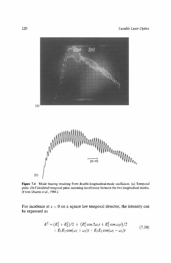
120 Tunable Laser Optics
Figure 7.4 Mode beating resulting from double-longitudinal-mode oscillation. (a) Temporal pulse. (b) Calculated temporal pulse assuming interference between the two longitudinal modes. (From Duarte et al., 1988.)
For incidence at z = 0 on a square law temporal detector, the intensity can be expressed as
E 2 - ( E 2 -+- E 2 ) / 2 + (E 2 cos 2w1 t -+- E 2 cos w21)/2
-k E1 E2 cos(col Jr- w2) t + E1 E2 cos(w1 - w2) t (7.10)

Pulsed Narrow-Linewidth Tunable Laser Oscillators 121
Detectors in the nanosecond regime respond only to the first and the last terms of this equation, so Eq. (7.10) can be approximated by
E 2 ~ (E~ + E2)/2 + E1E2 cos(~l - ~ 2 ) t (7.11)
Using this approximation and a non-Gaussian temporal representation derived from experimental data, for the amplitudes of the form
E1 (t) -- (a2t 2 + alt + ao)(blt + bo) -1 (7.12)
a calculated version of the experimental waveform exhibiting mode beating can be obtained as shown in Fig. 7.4b. For this particular dispersive oscillator lasing in a double longitudinal mode, the ratio of frequency jitter 5~ to cavity mode spacing A~ ~ (~l - ~2) was represented by a sinusoidal function at 20 MHz. The initial mode intensity ratio is 200:1 (Duarte et al., 1988; Duarte, 1990a).
In the case of SLM emission, the Fabry-Perot interferometric rings appear singular and well defined (see Fig. 7.5). Mode beating in the temporal domain is absent, and the pulses assume a near-Gaussian distribution (see Fig. 7.6). These results were obtained in an optimized solid-state multiple- prism grating dye laser oscillator for which A u A t ~ 1 (Duarte, 1999).
Figure 7.5 Fabry-Perot interferogram corresponding to single-longitudinal-mode emission at Au ~ 350 MHz. (From Duarte, 1999.)

122 Tunable Laser Optics
Figure 7.6 Near-Gaussian temporal pulse corresponding to single-longitudinal-mode emission. The temporal scale is 1 ns/div. (From Duarte, 1999.)
7.3 T U N A B L E L A S E R O S C I L L A T O R A R C H I T E C T U R E S
Tunable laser oscillators can be configured in a variety of cavity designs. Here, a brief survey of these alternatives is presented. In general, these cavity architectures can be classified into tunable laser oscillators without intracav- ity beam expansion and tunable laser oscillators with intracavity beam expansion (Duarte, 1991 a). Further, each of these classes can be divided into open- and closed-cavity designs (Duarte and Piper, 1980). It is assumed that oscillators considered in this section are designed to yield narrow-linewidth emission. The architectures are relevant to a variety of tunable gain media and are applicable to both CW and pulsed lasers.
7.3.1 TUNABLE LASER OSCILLATORS WITHOUT INTRACAVITY BEAM EXPANSION
Tunable laser oscillators without intracavity beam expansion are those laser resonators in which the intrinsic narrow beam waist at the gain region is not expanded using intracavity optics. The most basic of tunable laser designs is that incorporating an output mirror coupler and a tuning grating in Littrow configuration, as illustrated in Fig. 1.5. Tuning is accomplished by slight rotation of the grating. This cavity configuration will yield relatively broad

Pulsed Narrow-Linewidth Tunable Laser Oscillators 123
Figure 7.7 Grating-mirror tunable laser cavities. [Reprinted from Duarte (1995b), copyright 1995b, with permission from Elsevier].
tunable emission in a short pulsed laser, such as a high-power pulsed dye laser, but could emit fairly narrow emission if applied to a CW semiconduc- tor laser. A refinement of this cavity consists in inserting one or more intracavity etalons to further narrow the emission wavelength, as illustrated in Figs. 7.7 and 7.8. Such multiple-etalon grating cavities can yield very narrow-linewidth pulsed emission, down to the SLM regime, in high-power pulsed lasers. The introduction of the etalons provides further avenues of wavelength tuning. The main disadvantage of this class of resonator in the pulsed regime is the very high intracavity power flux that can induce optical damage in the grating and the coating of the etalons.
An important configuration in the tunable laser oscillators without intra- cavity beam expansion class that employs only the natural divergence of the intracavity beam for total illumination of the diffractive element is the grazing-incidence grating design (Shoshan et al., 1977; Littman and Metcalf,
Figure 7.8 Mirror-mirror laser cavity incorporating intracavity etalons.

124 Tunable Laser Optics
1978). In these lasers the grating is deployed at a high angle of incidence. The diffracted beam is subsequently reflected back toward the grating by the tuning mirror. A variation on this design is the replacement of the tuning mirror by a grating deployed in Littrow configuration (Littman, 1978). This cavity has been configured as an open cavity, as shown in Fig. 7.9a, or as a closed cavity, as shown in Fig. 7.9b. A further alternative is the inclusion of an intracavity etalon (Saikan, 1978) for further linewidth narrowing. Grazing-incidence grating cavities have the advantage of being fairly com- pact and are widely used both in the pulsed regime and in the CW regime. A limitation of these cavities is the relatively high losses associated with the deployment of the diffraction grating at a high angle of incidence, as illus- trated in Fig. 7.10 (Duarte and Piper, 1981).
For tunable laser oscillators without intracavity beam expansion and in the absence of intracavity etalons, the cavity linewidth equation takes the fairly simple form of
,/kA '~ AOR(RVAOG) -1 (7.13)
where V~Oa is the grating dispersion either in Littrow configuration,
Figure 7.9 Grazing-incidence grating cavities. (a) Open cavity. (b) Closed cavity. In these oscillators, the refraction angle identified as 0' corresponds to �9 [Reprinted from Duarte (1990a), copyright 1990, with permission from Elsevier].

Pulsed Narrow-Linewidth Tunable Laser Oscillators 125
50
4O >, O r
~
._~ 30 uJ
20
10
5
Grating efficiency
- I
I I I ~ , , , i , , 7 - ' ~ 1
60 70 80 85 90 Incidence Ange (|
Figure 7.10 Grating efficiency curve as a function of angle of incidence at A = 632.8 nm. (From Duarte and Piper, 1981.)
V~OG -- (2 tan O)/A
V,xOG -- m/(d cos O)
(7.14)
(7.15)
or in grazing-incidence configuration,
VAOG -- 2(sin O + sin ~ ) / (A cos O)
~7,~OG -- 2m/(d cos O)
(7.16)
(7.17)
where the multiple-return-pass beam divergence A0R is given by
AOR --(A/Trw) (1 + (L~/BR) 2 + (ARL~/BR) 2) 1/2 (7.18)
and the appropriate propagation terms can be calculated according to the optical architecture of the cavity, as described in Chapter 6.
For tunable oscillators incorporating a diffraction grating and an intra- cavity etalon, the linewidth established via Eq. (7.13) can be used to provide Au via Eq. (7.7) and thus to determine the free spectral range (FSR) of the etalon, which is given by (Born and Wolf, 1999)
F S R - c/2nle (7.19)
where n is the refractive index of the etalon's material and le is the distance between the reflective surfaces. The expression for the FRS has its origin in A u - c/Ax.

126 Tunable Laser Optics
The minimum resolvable linewidth or resulting laser linewidth obtainable from the etalon is given by
Ab'FR S - - F R S / ~ (7.20)
where ~ is the effective finesse of the etalon. The finesse of the etalon is a function of the flatness of the surfaces (often in the range of A/100 - A/50), the dimensions of the aperture, and the reflectivity of the surfaces. The effective finesse is given by (Meaburn, 1976)
OY -~-2 -- ~---~R 2 + ~ F 2 --I-- ~--~A 2 (7.21)
where ~ R , ~F, and ~ A are the reflective, flatness, and aperture finesses, respectively. The reflective finesse is given by (Born and Wolf, 1999)
~ g = ~-x/R/(1 - R) (7.22)
where R is the reflectivity of the surface. Further details on Fabry-Perot etalons are given in Chapter 11.
Multiple-etalon systems are described in detail in the literature (Maeda etal., 1975; Pacala etal., 1984). As implied earlier, these multiple-etalon assemblies are designed so that the FRS of the etalon to be introduced is compatible with the measured laser linewidth attained with the previous etalon or etalons. Although this is a very effective avenue to achieve fairly narrow linewidths, the issue of optical damage due to high intracavity power densities does introduce limitations. The performance of representative tunable laser oscillators without intracavity beam expansion is summarized in Table 7.1.
7 . 3 . 2 TUNABLE LASER OSCILLATORS WITH INTRACAVITY
BEAM EXPANSION
Equation 7.3 indicates that a key principle in achieving narrow-linewidth emission consists of augmenting the intrinsic intracavity dispersion provided by the diffraction grating. This is accomplished by the total illumination of the diffraction surface of the tuning element. In the case of the grazing- incidence grating cavities, this is done by deploying the grating at a high angle of incidence; however, that can be associated with low diffraction efficiencies. An alternative method is to illuminate the diffractive element via intracavity beam expansion. Tunable laser oscillators with intracavity beam expansion are divided into two subclasses: those using two-dimensional beam expansion and those using one-dimensional beam expansion.
Initially, intracavity beam expansion was accomplished utilizing two- dimensional beam expansion and a diffraction grating deployed in Littrow
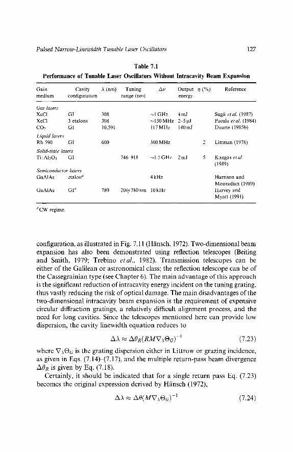
Pulsed Narrow-Linewidth Tunable Laser Oscillators 127
Table 7.1
Performance of Tunable Laser Oscillators Without Intracavity Beam Expansion
Gain Cavity A (nm) Tuning Au Output r/(%) Reference medium configuration range (nm) energy
Gas lasers XeC1 GI 308 H1 GHz 4 mJ XeC1 3 etalons 308 HI50 MHz 2-5 gJ CO2 G! 10,591 117 MHz 140mJ
Liquid lasers Rh 590 GI 600 300 MHz
Solid-state lasers Ti : A1203 G! 746-918 ~1.5 GHz 2 mJ
Semiconductor lasers GaA1As etalon a 4 kHz
GaA1As GI a 780 20@780nm 10kHz
Sugii et al. (1987) Pacala et al. (1984) Duarte (1985b)
Littman (1978)
Kangas et al. (1989)
Harrison and Mooradian (1989) Harvey and Myatt (1991)
a CW regime.
configuration, as illustrated in Fig. 7.11 (H/insch, 1972). Two-dimensional beam expansion has also been demonstrated using reflection telescopes (Beiting and Smith, 1979; Trebino etal., 1982). Transmission telescopes can be either of the Galilean or astronomical class; the reflection telescope can be of the Cassegrainian type (see Chapter 6). The main advantage of this approach is the significant reduction of intracavity energy incident on the tuning grating, thus vastly reducing the risk of optical damage. The main disadvantages of the two-dimensional intracavity beam expansion is the requirement of expensive circular diffraction gratings, a relatively difficult alignment process, and the need for long cavities. Since the telescopes mentioned here can provide low dispersion, the cavity linewidth equation reduces to
/ kA ~ A O R ( R M V ) ~ O G ) -1 (7.23)
where V~Oc is the grating dispersion either in Littrow or grazing incidence, as given in Eqs. (7.14)-(7.17), and the multiple return-pass beam divergence AOR is given by Eq. (7.18).
Certainly, it should be indicated that for a single return pass Eq. (7.23) becomes the original expression derived by H/insch (1972),
/k)~ ~ / k O ( M V ~ O G ) -1 (7.24)

128 Tunable Laser Optics
Figure 7.11 Two-dimensional transmission telescope Littrow grating laser cavity. (From Duarte, 1990a.)
One-dimensional intracavity beam expansion uses multiple-prism beam expanders rather than conventional telescopes to perform the beam expan- sion. Multiple-prism grating tunable laser oscillators are classified as multiple- prism Littrow (MPL) grating laser oscillators (Klauminzer, 1978; Kasuya et al., 1978; Wyatt, 1978; Duarte and Piper, 1980) and hybrid multiple-prism grazing-incidence (HMPGI) grating laser oscillators (Duarte and Piper, 1981, 1984a). The MPL and HMPGI grating laser oscillators are depicted in Figs. 7.12 and 7.13, respectively. Both of these oscillator subclasses belong to the closed-cavity class.
In these laser oscillators the intracavity beam expansion is one- dimensional, thus facilitating the alignment process significantly. In addition, the requirements on the dimensions of the diffraction grating perpendicular
Figure 7.12 Optimized compact MPL grating solid-state dye laser oscillator. (From Duarte, 1999.)
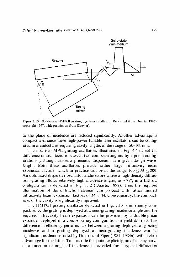
Pulsed Narrow-Linewidth Tunable Laser Oscillators 129
Solid-state gain medium
Grating _ ,, _~1 M ~
\\x[
! ( / Tuning '~ ~ ~ " mirror
Figure 7.13 Solid-state HMPG[ grating dye laser oscillator. [Reprinted from Duarte (1997), copyright 1997, with permission from Elsevier].
to the plane of incidence are reduced significantly. Another advantage is compactness, since these high-power tunable laser oscillators can be config- ured in architectures requiring cavity lengths in the range of 50-100 mm.
The first two MPL grating oscillators illustrated in Fig. 4.4 depict the difference in architecture between two compensating multiple-prism config- urations yielding near-zero prismatic dispersion at a given design wave- length. Both these oscillators provide rather large intracavity beam expansion factors, which in practice can be in the range 100 _< M <_ 200. An optimized dispersive oscillator architecture where a high-density diffrac- tion grating allows relatively high incidence angles, at ~77 ~ in a Littrow configuration is depicted in Fig. 7.12 (Duarte, 1999). Thus the required illumination of the diffraction element can proceed with rather modest intracavity beam expansion factors of M ~ 44. Consequently, the compact- ness of the cavity is significantly improved.
The HMPGI grating oscillator depicted in Fig. 7.13 is inherently com- pact, since the grating is deployed at a near-grazing-incidence angle and the required intracavity beam expansion can be provided by a double-prism expander deployed in a compensating configuration to yield M ~ 30. The difference in efficiency performance between a grating deployed at grazing incidence and a grating deployed at near-grazing incidence can be significant, as demonstrated by Duarte and Piper (1981, 1984a), with a clear advantage for the latter. To illustrate this point explicitly, an efficiency curve as a function of angle of incidence is provided for a typical diffraction

130 Tunable Laser Optics
grating in Fig. 7.10. It is interesting to note that most of external semicon- ductor lasers use the near-grazing-incidence configuration rather than the pure grazing-incidence scheme, given the highly divergent beams available from the narrow-gain regions of semiconductor lasers. The MPL and HMPGI grating oscillator configurations are directly applicable to tunable high-power gas lasers, such as excimer lasers and CO2 lasers (Duarte, 1985c), as depicted in Fig. 7.14.
The MPL and HMPGI grating oscillators have been shown to inherently yield extremely low levels of amplified spontaneous emission (ASE), which is a very desirable feature in many applications, including high-resolution spectroscopy (Duarte and Piper, 1980, 1981). The MPL and HMPGI grating oscillators described here incorporate a polarizer-output-coupler mirror that is antireflection coated toward the gain medium and whose output surface is broadband coated with ~20% reflectivity. The function of this polarizer- output coupler is to further suppress the single-pass amplified spontaneous emission, since the laser emission from these oscillators is intrinsically highly polarized parallel to the plane of incidence. Using these oscillator architec- tures, ASE levels, as determined by the spectral density ratio PASE/Pl (Duarte, 1990b), are in the 10-7-10 -6 range (Duarte, 1990b, 1997, 1999).
The multiple-return-pass linewidth for a multiple-prism grating oscillator is given by (Duarte and Piper, 1984b; Duarte, 2001)
A A - AOR(RMVa@o + R~7A~p) -1 (7.25)
Figure 7.14 MPL and HMPGI grating high-power pulsed C O 2 laser oscillators. (From Duarte, 1985c.)

Pulsed Narrow-Linewidth Tunable Laser Oscillators 131
where 27~Oc is the grating dispersion either in Littrow or grazing-incidence configuration, as given in Eqs. (7.14)-(7.17), and the multiple-return-pass beam divergence AOR is given by Eq. (7.18). In addition to the dispersion of the grating, the multiple prism must also be considered and is given by (Duarte and Piper, 1982; Duarte, 1985a, 1989)
-1
VAmp --2M1M2 Z ( • kid k2 j m=l =m "=
r m ) n t- 2 Z ( - + - l ) ~ 2 , m k l j I I k2j ~TAf/m
m=l =1 j=l
V,~nm
(7.26)
As indicated in Chapter 4, either Eq. (7.26) can be used to evaluate the return-pass multiple-prism dispersion or it can be applied to design a zero- dispersion beam expander at a given wavelength. In the latter case, VAff~p ~ 0 and Eq. (7.25) reduces to Eq. (7.23). As described in Chapter 5, the transmission efficiency of the multiple-prism beam expander can be quantified using
L1, m = L2,(m_l) + (1 - L 2 , ( m _ l ) ) ~ l , m
L2,m --- Ll,m + (1 -- L l,m) ~2 ,m
(7.27)
(7.28)
where L l,m and L2,m represent respectively, the losses at the incidence and exit surfaces of the mth prism. ~l,m and ~2,m are the respective Fresnel reflection factors given in Chapter 5. The performance of tunable laser oscillators with intracavity beam expansion is summarized in Table 7.2.
7.3.3 WIDELY TUNABLE NARROW-LINEWIDTH EXTERNAL-CAVITY SEMICONDUCTOR LASERS
The external-cavity semiconductor laser (ECSL) has become widely used in a number of contemporaneous applications, including laser cooling and Bose-Einstein condensation. Central to the attractiveness of ECSLs is their tunability, narrow-linewidth characteristics, stability, compactness, and low cost. Two of the most popular external-cavity configurations belong to the open-cavity class in the form of a Littrow grating cavity design (Wieman and Hollberg, 1991) and a grazing-incidence grating design (Harvey and Myatt, 1991). The adoption of open-cavity designs appears to have resulted from a need to adapt to the availability of commercial semiconductor lasers with one end of the cavity sealed from access.

132 Tunable Laser Optics
Table 7.2
Performance of Tunable Laser Oscillators with Intracavity Beam Expansion
Gain Cavity A (nm) Tuning Au Output r /(%) Reference medium configuration range (nm) energy
Gas lasers XeC1 HMPGI a 308 1.8 GHz CO2 MPL 10,591 140 MHz CO2 HMPGI 10,591 107 MHz Liquid dye lasers Rh 590 Telescopic 600 2.5 GHz Rh 590 Telescopic b 600 300 MHz C 500 MPL 510 490-530 1.61GHz
Rh 590 MPL b 572 60 MHz
Rh 590 MPL 575 565-605 1.4GHz
C 500 HMPGI 510 490-530 1.15GHz
Rh 590 HMPGI 575 565-603 400-650MHz
Solid-state dye lasers Rh 590 MPL 590 550-603 350MHz Rh 590 HMPGI 580 565-610 375MHz
Semiconductor lasers InGaAs MPG c 1255-1335 100 kHz
P/InP Diode a HMPGI 670
GaInP- Littrow e 640-652 A1GaInP
1.2 GHz a
4 MHz
Duarte (199 lb) 200 mJ Duarte (1985c)
85 mJ Duarte (1985c)
20 Hfinsch (1972) 2-4 Hfinsch (1972)
14 Duarte and Piper (1980)
5 Bernhardt and Rassmusen (1981)
5 Duarte and Piper (1984a)
4 Duarte and Piper (1981 )
4 Duarte and Piper (1984a)
5 Duarte (1999) 4 Duarte (1997)
Zorabedian (1992)
Duarte (1993b) Laurila et al. (2002)
,1 Calculated return-pass dispersive linewidth. b Includes intracavity etalon. c CW regime. aIndex guided. e Transmission grating.
The advantages of closed-cavity tunable laser oscillators over open-cavity alternatives in the pulsed high-power domain were outlined by Duarte and Piper (1980, 1981). These advantages include significantly reduced optical noise levels and independence from external feedback effects. Although the first phenomenon is less pronounced, in semiconductor lasers the second observation still applies. Moreover, in ECSLs incorporating open Littrow

Pulsed Narrow-Linewidth Tunable Laser Oscillators 133
grating configurations, the diffracted beam is directed back to the gain region while the output is coupled via the reflection losses of the grating. This means that as the wavelength is tuned, the direction of the output beam changes. Thus, additional external optics is required for beam correction (Hawthorn et al., 2001). In ECSLs incorporating the open grazing-incidence configur- ation, tighter boundaries for thermal stability are required (Laurila et al., 2002).
This is interesting, given the fact that closed-cavity ECSLs preceded the open-cavity alternatives (Voumard, 1977; Fleming and Mooradian, 1981; Belenov et al., 1983). The main difference is that ECSLs require access to both ends of the gain region. Ideally both ends of the gain region should be antire- flection coated, as indicated by Fleming and Mooradian (1981), so that the characteristics of the emission are entirely controlled by the external cavity, as illustrated in Fig. 7.15 (Duarte, 1993b). Alternatively, at least one of the cavity ends should be antireflection coated. When this is the case, the frequency- selective elements are deployed next to the antireflection end of the gain region and the laser output is coupled from the partially reflective extreme (Notomi et al., 1990).
Perhaps one of the most thoroughly engineered ECSLs to date is that reported by Zorabedian (1992), which was based on a closed-cavity
Figure 7.15 (a) MPL and (b) HMPGI grating semiconductor laser oscillators. In the HMPGI grating oscillator, the refraction angle identified as 0' corresponds to ff~ [from Duarte (1993b), reproduced with permission. Copyright Laser Focus World 2003].

134 Tunable Laser Optics
multiple-prism Littrow grating design. This author reports on a laser linewidth of Au = 100 kHz sustainable over a 60-nm tuning range, with a side-mode suppression ratio of 70 dB (Zorabedian, 1992).
The closed-cavity approach has recently gained further attention in the form of a cavity incorporating a transmission Littrow grating (Laurila et al., 2002). These authors report laser linewidths of Au ~ 4 MHz over a tuning range of 12nm centered at A - 646nm. The laser beam has an elliptical profile of 8 mm x 1.5 mm (Laurila et al., 2002). Elliptical TEM00 laser beam profiles are typical in semiconductor lasers, and they are a result of the rectangular cross section of the gain region. For instance, rectangular dimensions of 4 ~tm x 1 ~tm are not uncommon (Fox et al., 1997). One way to produce intracavity a circular beam with tunable narrow-linewidth charac- teristics is to introduce multiple-prism beam expansion prior to illumination of the transmission grating. In this design the gain region is oriented to emit its elliptical beam with the long axis perpendicular to the plane of incidence. The multiple-prism beam expander then elongates the narrow dimension of the beam to yield a circular profile incident on the grating. The beam expansion, which contributes to the line narrowing, takes place at a plane parallel to the plane of incidence. This cavity is depicted in Fig. 7.16. Comprehensive reviews on ECSLs are given by Zorabedian (1995), Duarte (1995c), and Fox et al. (1997).
7.3.4 DISTRIBUTED-FEEDBACK LASERS
A laser architecture that does not belong to either class of resonators previously described, since it does not incorporate mirrors in the optical axis of the emission, is that of the distributed-feedback (DFB) laser introduced by Kogelnik and Shank (1971). In these laser configurations, depicted in Fig. 7.17, the excitation laser beam is divided into two subbeams that are recombined at the gain medium, where they produce an interference signal.
Figure 7.16 MPL transmission grating semiconductor laser oscillator designed to produce circular TEM00 emission. The semiconductor is oriented to emit its elongated beam with the long axis perpendicular to the plane of propagation. Intracavity prismatic beam expansion (parallel to the plane of propagation) renders a nearly circular output beam.

Pulsed Narrow-Linewidth Tunable Laser Oscillators 135
Gain medium
\ \ \ " \ 0
/ / / / /
/
i i
i I
\ \
Figure 7.17 Distributed feedback laser [adapted from Shank etal. (1971)].
In DFB lasers, feedback is provided by backward Bragg scattering induced by the periodic perturbations of the refractive index at the gain medium. Kogel- nik and Shank (1972) have modeled basic gain and spectral features of these lasers using a representation of the scalar wave equation in the form of
(OZE/Oz 2) -k- nZE = 0 (7.29)
and a two-counter propagating-wave approach to describe the electric field in the form of
E(z) = R(z )e -i~z/2 + S(z )e inz/2 (7.30)
where z is in the direction of propagation. These authors also assume a periodic spatial variation in the refractive
index, represented by
n(z) = n + n: cos t~z (7.31)
where ~ is related to the fringe spacing A by
- 27r/A (7.32)

136 Tunable Laser Optics
and the wavelength of oscillation is defined by the Bragg condition
)V = 2nA (7.33)
The passive linewidth of a DFB laser is given by (Bor, 1979)
A)~ t= (,~t/Ap)A)~p (7.34)
where AI is the wavelength of the DBF laser, Ap is the wavelength of the pump laser, and AAp is the linewidth of the pump laser. This equation indicates that the linewidth of the DFB laser is determined by the spectral properties of the pump laser. Thus, narrow-linewidth emission in DBF lasers requires a narrow-linewidth pump laser. This is quite different from the lasers using dispersive oscillators whose emission linewidth is independent of the bandwidth of the excitation source.
Tuning DFB lasers can be accomplished either by varying the refractive index of the gain medium or by changing A. The refractive index can be changed by thermal means or by varying the composition of the gain medium. In the case of DFB dye lasers, that is done by altering the composition of the solvents. For a DFB laser configuration, allowing rotation of the mirrors, as shown in Fig. 7.17, the fringe separation is given by the first-order grating equation
A = Ap/2 sin 0 (7.35)
so (Shank et al., 197 l)
)~t = n~p/ sin 0 (7.36)
which allows the laser to be tuned by geometrical means. Given their typical linewidth characteristics, Au ~ 45 GHz (Bor, 1979),
DFB lasers are well-known sources of pulses in the picosecond regime. Distributed-feedback laser configurations originally applied to liquid dye lasers have also been demonstrated with solid-state dye laser gain media (Wadsworth et al., 1999; Zhu et al., 2000).
In the CW regime, DFB semiconductor lasers have been demonstrated to yield linewidths as low as 2 MHz in the wavelength range of 1.30-1.55 gm (Wolf et al., 1991).
7.4 W A V E L E N G T H - T U N I N G T E C H N I Q U E S
Laser oscillators incorporating dispersive, diffractive, and interferometric elements such as prisms, gratings, and etalons are intrinsically tunable. Here, several wavelength-tuning techniques based on these elements are described.
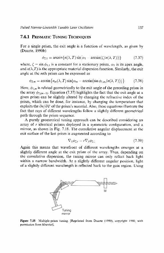
Pulsed Narrow-Linewidth Tunable Laser Oscillators 137
7.4.1 PRISMATIC TUNING TECHNIQUES
For a single prism, the exit angle is a function of wavelength, as given by (Duarte, 1990b)
~2,1 =- arcsin{n(A, T)sin[c~l - arcsin(~/n(A, T))]} (7.37)
where, ~ = sin ~51,1 is a constant for a stationary prism, c~1 is its apex angle, and n(A,T) is the appropriate material dispersion function. Similarly, the exit angle at the ruth prism can be expressed as
~52, m -- arcsin{nm(A, T)sin [C~m - arcsin(sin ~l,mln()~, r ) ) J } (7.38)
Here, q51,m is related geometrically to the exit angle of the preceding prism in the array q52,(m-1). Equation (7.37) highlights the fact that the exit angle at a given prism can be slightly altered by changing the refractive index of the prism, which can be done, for instance, by changing the temperature that exploits the On/OT of the prism's material. Also, these equations illustrate the fact that rays of different wavelengths follow a slightly different geometrical path through the prism sequence.
A purely geometrical tuning approach can be described considering an array of r identical prisms deployed in a symmetric configuration, and a mirror, as shown in Fig. 7.18. The cumulative angular displacement at the exit surface of the last prism is augmented according to
VAq52,r-- rVA02,1 (7.39)
Again this means that wavefront of different wavelengths emerges at a slightly different angle at the exit prism of the array. Thus, depending on the cumulative dispersion, the tuning mirror can only reflect back light within a narrow bandwidth. At a slightly different angular position, light of a slightly different wavelength is reflected back to the gain region. Using
Figure 7.18 Multiple-prism tuning. [Reprinted from Duarte (1990), copyright 1990, with permission from Elsevier].

138 Tunable Laser Optics
this approach, Strome and Webb (1971) report a tuning range from 571 to 615 nm using a four-prism sequence in a pulsed dye laser.
7.4.2 DIFFRACTIVE TUNING TECHNIQUES
Diffraction gratings are the main tuning elements in narrow-linewidth dis- persive laser oscillators. In a cavity incorporating a grating deployed in a grazing-incidence or near-grazing-incidence configuration (as illustrated in Fig. 7.19), the wavelength is changed by rotating the tuning mirror. Wave- length tuning in this configuration is described by the grating equation
mA = d(sin O + sin ~) (7.40)
where O is the angle of incidence and �9 is the angle of refraction. For a fixed angle of incidence, different wavelengths diffract at different angles. Hence the precise angular position of the tuning mirror determines the wavelength of the radiation that will return to the gain region for further amplification. Geometrically, the tuning is described by Eq. (7.40), where m, d, and O are kept constant so that A becomes a function of sin ~.
For a grating in Littrow configuration, O = �9 (see Fig. 7.20) and the grating equation becomes
mA -- 2d sin 0 (7.41 )
With m and d fixed, A becomes solely a function of sin O. Using these simple diffraction techniques, narrow-linewidth dispersive laser oscillators have been tuned over 50 nm or more (Duarte, 1990a, 1999).
Accurate angular displacement of tuning gratings requires the use of high- quality kinematic mounts with 0.1 s of arc or better. For a MPL grating oscillator, a frequency shift of 6u ~ 250 MHz, equivalent to the Au of the
" ~~,~ning mirror
Grating Figure 7.19 Diffraction grating deployed in near-grazing-incidence configuration.

139
/ / /
/
Pulsed Narrow-Linewidth Tunable Laser Oscillators
Figure 7.20 Diffraction grating deployed in Littrow configuration.
dispersive oscillator, requires an angular rotation of 60 ~ 10 -6 radians at the grating (Duarte et al., 1988).
7.4.3 INTERFEROMETRIC TUNING TECHNIQUES
In addition to prismatic and diffractive tuning methods, intracavity etalons provide a further alternative for fine wavelength tuning. According to Born and Wolf (1999) the etalon can be considered a periodic-wavelength filter that satisfies the condition
me)~ = 2n(A, T)de cos Ce (7.42)
for maxima. Here, me is an integer, de is the distance between the reflective surfaces, ~e is the refraction angle that is related to the tilt angle by
sin ~e = n(A, T) sin ~e (7.43)
and n(A,T) is the refractive index of the substrate of the etalon (see Fig. 7.21). The angular dispersion of the etalon can be written as (Duarte, 1990b)
VA(~e = (sin//)e/COS ~e)VAn + n(COS if)e/COS ~e)VA~/) e (7.44)
where
VA?/)e -- ( n - l V A r/ -- A-1) (tan //)e) -1
For n = 1 the condition VA(~e = ~7A?/Je arises, so
VA~e -- --(A tan ~be) -1
(7.45)
(7.46)

140 Tunable Laser Optics
Figure 7.21 Solid etalon depicting incidence and refraction angles.
as given by ScMfer (1990). For the special case of n -- 1, it can be shown that the wavelength shift resulting from a displacement in ~be (from 4~e = 0 at A1) is given by (Sch~ifer, 1990)
~)k ~" ( | -- COS (~e),,~l (7 .47)
In addition to angular rotation, an alternative fine tuning technique exploits the thermal dependence of the refractive index of the etalon's substrate. Using Eq. (7.42), the wavelength difference from A1 to A2, corresponding to a change in temperature from/ '1 to T2, can be written as
6A -- (21e/me)(n( T1) cOS ~el - n( T2) cOS ~e2)
which for ~e~ = 0 at A1 reduces to
6)~ = (1 - - ( n ( Z 2 ) / n ( Z l ) ) C O S ~ e 2 ) ) ~ l
(7.48)
(7.49)
For the special case of n(T1) = n(T2) = 1 this equation reduces to Eq. (7.47). In addition to solid etalons, gas-spaced Fabry-Perot interferometers can
be used for fine frequency tuning. According to Meaburn (1976), the refrac- tive index of the gas can be varied as a function of pressure according to
K A P ~ n - 1 (7.50)
where K is a constant related to the intrinsic properties of the gas and AP is the pressure gradient applied over the plates of the interferometer. The wavelength shift thus obtained can be expressed as (Meaburn, 1976)
8A ,~ K A A P (7.51)
This principle was applied by Wallenstein and H~insch (1974) to vary the frequency of a telescopic dye laser oscillator, including a tilted etalon and a grating mounted in Littrow configuration. According to these authors the laser frequency changes almost linearly as a function of pressure according to
6u ~ - ( c / A ) K A P (7.52)

Pulsed Narrow-Linewidth Tunable Laser Oscillators 141
7 .4 .4 LONGITUDINAL TUNING TECHNIQUES
Tuning can also be done by changing the cavity length. This principle is based on the interferometric identity
6A = A2/cSx (7.53)
which can also be stated as
6u = c/6x (7.54)
Assume that the cavity linewidth AA remains constant at two relatively close but different wavelengths, as illustrated in Fig. 7.22. This is a reasonable assumption for a laser emitting a diffraction-limited beam. Under those circumstances the spacing of the intracavity modes will change within the transmission window, so
or
For AA1 ~ A/~2,
8 A 1 - A2/2L (7.55)
6A2 - A22/2(L + AL) (7.56)
N1 -- AA1/6A1 (7.57)
N2 -- A ) k 2 / ~ 2 (7.58)
)k2 ~ )kl(6)k2/6)kl)l/2(1 + (/kL/L)) 1/2 (7.59)
-~ A X , 1 ~-
Figure 7.22 Dispersive cavity linewidth at two slightly different frequencies. It is assumed that AA1 ,~ AA2 while the intracavity free spectral range changes.

142 Tunable Laser Optics
Or
A2 ~ AI(N1/N2)I/2(1 4-(AL/L)) 1/2 (7.60)
for AL = 0,6A1 = 6A2, and A1 ~ A2. For multilongitudinal-mode oscillation, this approach requires counting the number of modes at the two wave- lengths. For single-longitudinal-mode oscillation, N1 -- N2 = 1 and
A2 ,-~ AI(1 • (AL/L)) 1/2 (7.61)
This equation indicates that tuning, by changing the cavity length, depends on the AL/L ratio. For instance, a tunable dispersive oscillator yielding single- longitudinal-mode emission (Au ~ 350 MHz) with a cavity length of 75 mm (Duarte, 1999) can tune its emission wavelength from 590.0000nm to 590.2949 nm by increasing its cavity length by just 0.0750 mm. This wavelength change translates to a frequency shift of 253.9979 GHz. Given a laser linewidth of Au ~ 350 MHz, such change in cavity length translates into an enormous frequency shift. This implies that the cavity length of such oscillators must be carefully controlled to ensure stability in the frequency domain. For the case of a miniature laser cavity with a length of 1 mm, tuned with MEMS methods, and lasing at 650nm, the frequency can be tuned in steps of 2.3 GHz by changing the cavity length every 10 nm.
It should be noted that Eq. (7.61) applies over the limited tuning range where the condition AA1 ~ A)k2 holds. Uenishi etal. (1996) report on a MEMS-driven semiconductor laser with a cavity length L ~ 305 ~tm. For a change in cavity length of ~1 ~tm, these authors report a nearly linear change in wavelength of ~2.5 nm. Substituting AL ~ -1 ~tm and A1 ~ 1550nm into Eq. (7.61) yields A2 ~ 1547.45 nm, which agrees fairly well with an experi- mental value of A2 ~ 1547.50 nm.
7.4.5 SYNCHRONOUS TUNING TECHNIQUES
As the wavelength of the oscillator is being tuned using a dispersive element such as a diffraction grating, either in grazing-incidence or Littrow configuratrion, the FSR of the cavity or the spacing of the longitudinal modes varies according to
FSR = AZ/2L (7.62)
This can lead to abrupt jumps in the longitudinal-mode selection, which is also known as mode hopping. One way to suppress this effect is to adjust the cavity length accordingly so that the FSR of the cavity is not altered. This is known as synchronous tuning. In cavities tuned by a grating deployed in Littrow config-

Pul sed N a r r o w - L i n e w i d t h Tunab le Laser Osci l la tors 143
uration, synchronous tuning can be achieved by synchronizing the position of the output coupler mirror with the rotation of the grating. Although this is a simple principle, its successful practical implementation requires the applica- tion of accurate wavelength monitoring and high-precision servomechanisms.
An alternative approach to synchronous wavelength tuning, applicable to single-longitudinal-mode lasers, was introduced by Liu and Littman (1981), who realized that the cavity length (see Fig. 7.23) is an integral number of half-wavelengths, so
= (2/N)(Lu + Lp sin ~) (7.63)
where N is the number of longitudinal modes. Comparison of this equation with
A = (d/m)(sin 0 + sin ~)
indicates that equivalence is achieved if (Liu and Litmann, 1981)
2Lf / N = (d/m) sin
and
(7.64)
2 L p / N = (d/m) (7.65)
i / . / I
/ I J / I
L p / I 2 \ , / \~ I . I ~ ~t~ -41,/ r - ~ 1~
/ - / /
/ / / /
Gain me6ium ~ M
~t l.. t ) .
Figure 7.23 Synchronous wavelength tuning [adapted from Liu and Littman (1981)].

144 Tunable Laser Optics
Careful selection of the cavity parameters involved in these equations can lead to the establishment of a fairly wide single-mode scanning range. This scheme requires high-precision rotation of the tuning mirror, since the mechanical displacement equivalent to half a wavelength can result in mode hopping (Liu and Littman, 1981).
7.5 P O L A R I Z A T I O N M A T C H I N G
The polarization characteristics of a given tunable laser oscillator depend on the intrinsic polarization of the gain medium, the angle of the laser windows (or emission exit surfaces), the configuration of the dispersive elements, and the diffraction grating. For optimum laser conversion efficiency it is import- ant to perform a polarization matching of the gain region to that of the optical elements integrating the laser cavity. For the purpose of this discus- sion the plane of incidence is as defined in Chapter 5.
The polarization characteristics of a given gain medium depend on the atomic or molecular composition of such medium. A gain medium such as a laser dye responds differently to different orientations of the polarization of the pump laser (Sch~ifer, 1990). As illustrated in Fig. 7.22 (Duarte, 1990b), excitation with the pump laser beam polarized perpendicular to the plane of propagation yields single-pass emission also polarized perpendicular to the plane of incidence when using rhodamine 590 molecules as the gain medium and the 2P3/2-2D5/2 transition of the copper laser ( A - 510.554nm) as the excitation radiation. On the other hand, for excitation parallel to the plane of incidence the emission is almost unpolarized.
The first opportunity to induce a given polarization is presented in the selection of the angle of the laser windows. Windows deployed at an angle, thus creating a gain region in form of a trapezoid, greatly reduce internal reflections, contribute significantly to reducing optical noise, and facilitate the control of the spectral characteristics by the dispersive optics. The reflection losses for the given components of polarization are given by (Born and Wolf, 1999)
~11 - tan2(~ b - ~)/tanZ(q 5 + ~) (7.66)
~ • - sinZ(q~ - ~)/sinZ(~b + ~) (7.67)
For a multiple-prism grating oscillator, the reflection losses at the multiple- prism beam expander are calculated using Eqs. (7.27) and (7.28). The polarization efficiency response of a typical holographic grating suitable for linewidth narrowing and tuning in dispersive tunable laser oscillators is illustrated in Fig. 7.10.

Pulsed Narrow-Linewidth Tunable Laser Oscillators 145
Given that the polarization efficiency response of the grating clearly favors radiation polarized parallel to the plane of incidence and that the natural deployment of the multiple-prism beam expander (see Fig. 7.12) also induces a polarization parallel to the plane of incidence, it is logical to deploy the gain medium as illustrated in Fig. 7.24, that is, with the windows at an angle relative to the orthogonal to the optical axis and the trapezoid parallel to the plane of incidence. As described on Chapter 5, the closer this angle gets to Brewster's angle, the greater the preference for radiation polarized parallel to the plane of incidence. Finally, the orientation of the polarization of the excitation laser should be selected so that the single-pass emission is compatible with the polarization preference of the architecture of the oscillator. In this particular case, the pump laser radiation should be selected to yield unpolarized single-pass emission, as shown in Fig. 7.24b.
Using the approach described here, Duarte and Piper (1984a) demon- strated single-longitudinal-mode emission ~100% polarized parallel to the plane of incidence in a high-pulse-repetition-frequency copper-laser pumped dye laser. Polarization matching of the excitation laser to the polarization preference of the multiple-prism grating oscillator yields an increase of 15 % in the laser conversion efficiency (Duarte and Piper, 1984a). It should be indicated that although a specific example was used to describe the idea of polarization matching, the simple principles given are applicable to any laser
Figure 7.24 Polarization matching. [Reprinted from Duarte (1990b), copyright 1990, with permission from Elsevier].

146 Tunable Laser Optics
system and even to extracavity optics for the efficient transmission of laser radiation.
7.6 DESIGN OF EFFICIENT NARROW-LINEWIDTH T U N A B L E L A S E R O S C I L L A T O R S
The design of efficient optically pumped pulsed high-power tunable laser oscillators follows a well-defined series of stages, which are outlined here in chronological order.
1. Select the most efficient pump laser for the given medium. In the case of molecular gain media, the efficiency follows approximately the ratio (Shank, 1975)
T] ~ )ke/)k p (7.68)
where )~e is the emission wavelength and ~p is the wavelength of the pump source. In addition to better efficiency, in the case of visible dye lasers an excitation source with a wavelength close to the emission wavelength enhances significantly the lifetime of the gain medium. Specifically, the lifetimes of rhodamine dye solutions using copper-vapor-laser excitation is vastly superior to the lifetime of the same molecular medium under the excitation of ultraviolet lasers.
2. Determine the energy density threshold for optical damage of the gain medium.
3. Select the geometry of the gain medium. A trapezoid geometry is recommended to eliminate internal reflections and thus to facilitate the frequency control with the intracavity optics.
4. Once the approximate cavity length has been determined, select the dimensions of the beam waist (w) at the gain region adequate to yield TEM00 emission. This could be done applying Eqs. (7.1)-(7.3) or experimentally. An important issue here is not to exceed the energy density threshold for optical damage of the gain medium. For a given cavity length, verify experimentally that TEM00 emission is present.
5. Select the cavity architecture that best matches the application. Here, issues of compactness, simplicity, and efficiency play an important role.
6. Select an efficient high-density diffraction grating suitable for the requited tuning range. Use Eqs. (7.14)-(7.17) to determine the dispersion and Eqs. (7.40) and (7.41) to calculate the tuning range of a given grating.

Pulsed Narrow-Linewidth Tunable Laser Oscillators 147
~
.
.
10.
11.
12.
13.
If intracavity beam expansion is required, select the appropriate method of expansion. For telescopic beam expansion, use the matrix equations in Chapter 6 to design an appropiate two-dimensional beam expander. If a multiple-prism beam expander is selected, use Eq. (7.26) to design the multiple-prism array and Eqs. (7.27) and (7.28) to determine its transmission efficiency. The beam expander selected should have polar- ization characteristics compatible with those of the diffraction grating. Perform a return-pass linewidth calculation using Eq. (7.25). Adjust the cavity length to satisfy the criterion established in inequality (7.8). If the dispersion of the cavity is not sufficient to satisfy the criterion in inequality (7.8), either redesign the oscillator to attain a shorter cavity or insert an intracavity etalon. The etalon can be designed using Eqs. (7.19)-(7.22). Depending on the optical components integrating the cavity, select the method of wavelength tuning. Determine the polarization preference of the cavity and compare it to the polarization of the excitation source. Perform polarization matching if necessary. Determine the PASE/P! ratio. If necessary, replace the output-coupler mirror by a polarizer-output-coupler mirror, as illustrated in Fig. 7.12. Optimize alignment, and measure the conversion efficiency, tuning range, A0, and AA. If SLM oscillation is not observed, either decrease the cavity length or increase the intracavity dispersion.
7.6.1 USEFUL AXIOMS FOR THE DESIGN OF NARROW-LINEWIDTH TUNABLE LASER OSCILLATORS
A dispersive narrow-linewidth tunable laser oscillator integrates the follow- ing principles of optics in a single physical device: absorption, emission, interference, reflection, refraction, dispersion, and diffraction. As such, the design of efficient narrow-linewidth tunable laser oscillators does benefit from the careful application of a number of well defined, and specific, rules of physics which can be classified as follows:
1. The longer the cavity and the narrower the beam waist, the better the beam quality of the laser emission, or
I<xlx>l 2 - ~ ~(r j) 2 q- 2 ~ ~(rj) ~(rm)COS(am -- ~j) m=j+l

148 Tunable Laser Optics
2. The larger the optical length of the cavity, the lower the beam divergence, or
1/2 A0R --(A/Trw)(1 + (L~/BR) 2 + (ARL~/BR) 2)
3. For diffraction-limited TEM00 emission, the narrower the beam waist w, the larger the beam divergence, or
AO = A/Trw
4. The larger the beam magnification, the larger the intracavity dispersion and the narrower the linewidth, or
/XA -- A O R ( R M V , x O G -+- R V A ~ p ) -1
5. Also, from the previous axiom, the lower the beam divergence, the narrower the linewidth.
6. From the second and fourth axioms, the larger the number of intracavity passes, the lower the beam divergence and the narrower the linewidth.
7. The shorter the cavity, the longer the longitudinal-mode spacing, or
&, = c / 6 x
These axioms clearly illustrate that some of the design parameters have a competing effect on the overall physics. The task of the designer is to apply these principles in a balanced approach to optimize the beam divergence and linewidth performance in a compact-cavity architecture.
7.7 N A R R O W - L I N E W I D T H OSCILLATOR-AMPLIFIERS
The dispersive tunable laser oscillators so far described yield single- longitudinal-mode emission at very low levels of ASE. However, for many applications high energies or high-average powers are required. For that purpose the exquisite emission from the oscillator must be amplified by one or several amplification stages. A review on this subject and its literature is given by Duarte (1990b). Here, the focus will be on the fundamentals and the performance of various representative systems.
7.7.1 LASER-PUMPED NARROW-LINEWIDTH OSCILLATOR-AMPLIFIER CONFIGURATIONS
Amplification of coherent optical radiation in laser-excited systems is well illustrated by the configurations developed for dye lasers. Two of the most

Pulsed Narrow-Linewidth Tunable Laser Oscillators 149
interesting features of these systems is that amplification is performed in a single pass and that several stages of amplification are often employed. As such, given that lasing in these systems occurs in the nanosecond regime, it is important to synchronize the arrival of the oscillator pulse with the excita- tion of the amplifier. This is arranged by allowing the excitation geometry to delay the pump pulse, as illustrated in Fig. 7.25. An additional aspect important to the design of multistage oscillator-amplifier systems is the geometrical matching of the oscillator or preamplified beam with the focused excitation laser at the corresponding amplifier stage. This helps to maintain the cumulative ASE at low levels. For optimum efficiency, proper distribu- tion of the pump energy is required, with only a fraction (often less than 5 %) of it used to excite the oscillator. Correct polarization matching is also important.
The performances of illustrative multistage oscillator-amplifier laser sys- tems are listed in Table 7.3. Bos (1981) reports 6% efficiency at the oscillator, 20% at the preamplifier, and 60% at the amplifiers. The overall gain factor is about 229. The copper-vapor-laser pumped dye laser reported from Lawrence Livermore (Bass et al., 1992) operates at a pulse-repetition frequency of 13.2 kHz and comprises several master-oscillator power-amplifier (MOPA) chains performing at a 50-60% overall conversion efficiency. The master oscillators are of the MPL grating class and incorporate an intracavity etalon, and each MOPA chain includes three to four amplifiers in series.
Although most oscillator-amplifiers systems considered here utilize high- performance pulsed master oscillators, the alternative of semiconductor laser oscillators lasing in the CW regime is also available, as demonstrated
Tunable oscillator
AC1 AC2 ACa F F
BSO
beam
Figure 7.25 Single-pass multiple-stage laser amplifier.

150 Tunable Laser Optics
Table 7.3
Performance of Laser-Pumped Narrow-Linewidth Oscillator-Amplifier Configurations
Oscillator A (nm) Au configuration
Amplification Gain Output Output r/(%) Reference stages energy a power b
Telescopic c 590 320 MHz 3 229 165 mJ HMPGI 440 650MHz 2 ~700 3.5mJ
MPU ~590 0.5-5 GHz 3-4 d
a Per pulse. b Average power. e Includes intracavity etalon. dAt each of four amplification chains.
55 Bos (1981) ~9 Dupre
(1987) 2.5 kW@ 50-60 Glass et al. 13.2 kHz (1992)
by Farkas and Eden (1993). These authors used a five-stage dye laser amplification system to produce pulses of 1.2mJ at 786nm, with Av = 118 MHz.
7 .7 .2 NARROW-LINEWIDTH MASTER-OSCILLATOR FORCED-
OSCILLATOR CONFIGURATIONS
The master oscillator (MO) comprises the narrow-linewidth dispersive laser oscillators already discussed. The forced oscillator (FO), on the other hand, is an amplifier stage comprising a gain region within a resonator, as depicted in Fig. 7.26. The resonator of the amplifier stage can be an unstable reso- nator. Several aspects are rather critical to the efficient frequency locking of these configurations. First, the alignment of the master oscillator relative to the forced oscillator must be concentric. Second, there are stringent require-
Figure 7.26 Master-oscillator forced-oscillator laser configuration. (From Duarte and Conrad, 1987.)

Pulsed Narrow-Linewidth Tunable Laser Oscillators 151
ments on the timing of the excitation that impose arrival of the master- oscillator pulse at the onset of the forced-oscillator pulse buildup. Efficient frequency locking also occurs. Optimum lasing is achieved when the emis- sion wavelength of the master oscillator is tuned to the central wavelength of the gain spectrum of the forced oscillator. The performance of some repre- sentative master-oscillator forced-oscillator systems is described on Table 7.4.
The forced-oscillator cavity depicted in Fig. 7.26 is configured after a Cassegrainian telescope and is cataloged as a confocal unstable resonator of the positive branch (Siegman, 1986). Here the radius of curvature of the large concave mirror is R2, and the radius for the small mirror is R1 and has a negative value. The magnification of the resonator is given by (Siegman, 1986)
M - - ( R z / R 1 ) (7.69)
and its length is
L - - (R1 + R2)/2 (7.70)
As discussed by Siegman (1986), the condition for oscillation in the unstable regime is satisfied by
I(A + O)/21 > 1 (7.71)
where A and D are the matrix elements introduced in Chapter 6. For the resonator depicted in Fig. 7.26, R 1 - - 2 m and R 2 - 4m, so M - 2 and L - 1 m, and the condition for lasing in the unstable regime is satisfied.
Table 7.4
Performance of Narrow-Linewidth Master-Oscillator Forced-Oscillator Configurations
MO A (nm) Av configuration
FO Gain Output energy a Reference configuration
Two etalons 589
MPL 590
CW dye laser
aPer pulse.
346 MHz Flat-mirror cavity
<375 MHz Unstable resonator
80 MHz Ring cavity
~51
300 mJ Flamant et al. (1984)
600 mJ Duarte and Conrad (1987)
50 mJ Blit et al. (1977)

152 Tunable Laser Optics
PROBLEMS
1. For a laser emitting at )~ = 590 nm with a beam waist of 100 ~tm and a cavity length of 10cm, calculate the Fresnel number. Comment on the likely beam profile of this laser.
2. For a dispersive oscillator lasing with a TEM00 beam profile at )~ = 590 nm and a cavity length of 10 cm, calculate the longitudinal-mode spacing. Assuming that the calculated single-return-pass dispersive line- width is 1 GHz, determine whether this oscillator design is likely to yield single-longitudinal-mode emission, given that the temporal pulse is known to be 5 ns long at FWHM.
3. For a dispersive laser oscillator yielding double longitudinal-mode emis- sion with 6u = 1 GHz, design a suitable etalon to restrict oscillation to a single longitudinal mode. Assume a fairly high surface finesse and neglect the aperture finesse. Select a suitable reflection to allow maximum trans- mission while restricting oscillation to an SLM.
4. For a multiple-prism grating laser oscillator with w = l l7~tm and M = 100, calculate the single-return-pass linewidth for a 5-cm grating with 3000 l/mm. Assume )~ = 590nm, a diffraction-limited laser beam, and that the multiple-prism expander was designed to yield zero disper- sion at this wavelength.
5. For an etalon, from Eq. (7.42) derive Eq. (7.49) and then Eq. (7.47). 6. For an optimized tunable laser oscillator with a cavity length of 50mm
and lasing in an SLM at )~ = 590 nm, calculate the wavelength shift due to a decrease of 50 ~tm in cavity length.
7. Design, step by step, a multiple-prism grating oscillator capable of yield- ing SLM lasing at )~ = 590 nm. Assume that a beam waist of 100 ~tm can be attained at the gain region and that a 5-cm grating is available that has 3300 l/mm. Use a double-prism beam expander and configure it to yield zero dispersion at the given wavelength. Select a cavity length providing a longitudinal-mode spacing approximately equal to the return-pass linewidth.
REFERENCES
Bass, I. L., Bonanno, R. E., Hackel, R. H., and Hammond, P. R. (1992). High-average power dye laser at Lawrence Livermore National Laboratory. Appl. Opt. 31, 6993-7006.
Beiting, E. J., and Smith, K. A. (1979). An on-axis reflective beam expander for pulsed dye laser cavities. Opt. Commun. 28, 355-358.
Belenov, E. M., Velichanskii, V. L., Zibrob, A. S., Nitikin, V. V., Sautenkov, V. A., and Uskov, A. V. (1983). Methods for narrowing the emission line of an injection laser. Soy. J. Quantum Electron. 13, 792-798.

Pulsed Narrow-Linewidth Tunable Laser Oscillators 153
Bernhardt, A. F., and Rasmussen, P. (1981). Design criteria and operating characteristics of a single-mode pulsed dye laser. App. Phys. B 26, 141-146.
Blit, S., Ganiel, U., and Treves, D. (1977). A tunable, single-mode, injection-locked, flashlamp- pumped dye laser. Appl. Phys. 12, 69-74.
Bor, Zs. (1979). A novel pumping arrangement for tunable single picosecond pulse generation with a N2 laser pumped distributed feedback dye lasers. Opt. Commun. 29, 103-108.
Born, M., and Wolf, E. (1999). Principles of Optics, 7th ed. Cambridge University Press, Cambridge, UK.
Bos, F. (1981). Versatile high-power single-longitudinal-mode pulsed dye laser. Appl. Opt. 20, 1886-1890.
Duarte, F. J. (1985a). Note on achromatic multiple-prism beam expanders. Opt. Commun. 53, 259-262.
Duarte, F. J. (1985b). Application of dye laser techniques to frequency selectivity in pulsed CO2 lasers. In Proceedings of the International Conference on Lasers '84 (Corcoran, K. M., Sullivan, M. D., and Stwalley, W. C., eds.). STS Press, McLean, VA., pp. 397-403.
Duarte, F. J. (1985c). Multiple-prism Littrow and grazing-incidence pulsed CO2 lasers. Appl. Opt. 24, 1244-1245.
Duarte, F. J. (1989). Transmission efficiency in achromatic nonorthogonal multiple-prism laser beam expanders. Opt. Commun. 71, 1-5.
Duarte, F. J. (1990a). Narrow-linewidth pulsed dye laser oscillators. In Dye Laser Principles (Duarte, F. J., and Hillman, L. W., eds.) Academic Press, New York, pp. 133-183.
Duarte, F. J. (1990b). Technology of pulsed dye lasers. In Dye Laser Principles (Duarte, F. J., and Hillman, L. W., eds.). Academic, New York, pp. 239-285.
Duarte, F. J. (1991). Dispersive dye lasers. In High-Power Dye Lasers (Duarte, F. J., ed.). Springer-Verlag, Berlin, pp. 7-43.
Duarte, F. J. (1991b). Dispersive excimer lasers. In Proceedings of the International Conference on Lasers '90 (Harris, D. G., and Herbelin, J., eds.). STS press, McLean, VA, pp. 277-279.
Duarte, F. J. (1993a). On a generalized interference equation and interferometric measurements. Opt. Commun. 103, 8-14.
Duarte, F. J. (1993b). Multiple-prism grating designs tune diode lasers. Laser Focus Worm 29(2), 103-109.
Duarte, F. J. (1995a). Interferometric imaging. In Tunable Laser Applications (Duarte, F. J., ed.). Marcel Dekker, New York, pp. 153-178.
Duarte, F. J. (1995b). Narrow-linewidth laser oscillators and intracavity dispersion. In Tunable Lasers Handbook (Duarte, F. J., ed.). Academic Press, New York, pp. 9-32.
Duarte, F. J. (1995c). Dispersive external-cavity semiconductor lasers. In Tunable Laser Applications (Duarte, F. J., ed.). Marcel Dekker, New York, pp. 83-112.
Duarte, F. J. (1997). Multiple-prism near-grazing-incidence grating solid-state dye laser oscillator. Opt. Laser Technol. 29, 513-516.
Duarte, F. J. (1999). Multiple-prism grating solid-state dye laser oscillator: optimized architec- ture. Appl. Opt. 38, 6347-6349.
Duarte, F. J. (2001). Multiple-return-pass beam divergence and the linewidth equation. Appl. Opt. 40, 3038-3041.
Duarte, F. J., and Conrad, R. W. (1987). Diffraction-limited single-longitudinal-mode multiple- prism flashlamp-pumped dye laser oscillator: linewidth analysis and injection of amplifier system. Appl. Opt. 26, 2567-2571.
Duarte, F. J., and Piper, J. A. (1980). A double-prism beam expander for pulsed dye lasers. Opt. Commun. 35, 100-104.
Duarte, F. J., and Piper, J. A. (1981). Prism preexpanded grazing-incidence grating cavity for pulsed dye lasers. Appl. Opt. 20, 2113-2116.

154 Tunable Laser Optics
Duarte, F. J., and Piper, J. A. (1982). Dispersion theory of multiple-prism beam expanders. Opt. Commun. 43, 303-307.
Duarte, F. J., and Piper, J. A. (1984a). Narrow-linewidth, high-prf copper laser-pumped dye laser oscillators. Appl. Opt. 23, 1391-1394.
Duarte, F. J., and Piper, J. A. (1984b). Multi-pass dispersion theory of prismatic pulsed dye lasers. Optica Acta 31, 331-335.
Duarte, F. J., Ehrlich, J. J., Patterson, S. P., Russell, S. D., and Adams, J. E. (1988). Linewidth instabilities in narrow-linewidth flashlamp-pumped dye laser oscillators. Appl. Opt. 27, 843-846.
Dupre, P. (1987). Quasiunimodal tunable pulsed dye laser at 440nm: theoretical development for using quad prism beam expander and one or two gratings in a pulsed dye laser oscillator cavity. Appl. Opt. 26, 860-871.
Farkas, A. M., and Eden, J. G. (1993). Pulsed dye laser amplification and frequency doubling of single-longitudinal-mode semiconductor lasers. IEEE J. Quantum Electron. 29, 2923-2927.
Flamant, P. H., and Maillard, D. J. M. (1984). Transient injection frequency-locking of a microsecond-pulsed dye laser for atmospheric measurements. Opt. Quantum Electron. 16, 179-182.
Fleming, M. W., and Mooradian, A. (1981). Spectral characteristics of external-cavity controlled semiconductor lasers. IEEE J. Quantum Electron. QE-17, 44-59.
Fox, R. W., Hollberg, L., and Zibrov, A. S. (1997). Semiconductor diode lasers. In Atomic, Molecular, and Optical Physics: Electromagnetic Radiation (Dunning, F. B., and Hulet, R. G., eds.). Academic Press, New York, pp. 77-102.
Glass, I. L., Bonanno, R. E., Hackel, R. H., and Hammond, P. R. (1992). High-average power dye laser at Lawrence Livermore National Laboratory. Appl. Opt. 31, 6993-7006.
H~insch, T. W. (1972). Repetitively pulsed tunable dye laser for high-resolution spectroscopy. Appl. Opt. 11, 895-898.
Harrison, J., and Mooradian, A. (1989). Linewidth and offset frequency locking of external cavity GaA1As lasers. IEEE J. Quantum Electron. QE-25, 1152-1155.
Harvey, K. C., and and Myatt, C. J. (1991). External-cavity diode laser using a grazing- incidence diffraction grating. Opt. Lett. 16, 910-912.
Hawthorn, C. J., Weber, K. P., and Scholten, R. E. (2001). Littrow configuration tun- able external-cavity diode laser with fixed-direction output beam. Rev. Sci. Instrum. 72, 4477-4479.
Kangas, K. W., Lowenthal, D. D., and Muller, C. H. (1989). Single-longitudinal-mode, tunable, pulsed Ti:sapphire laser oscillator. Opt. Lett. 14, 21-23.
Kasuya, T., Suzuki, T., and Shimoda. K. (1978). A prism anamorphic system for Gaussian beam expander. Appl. Phys. 17, 131-136.
Klauminzer, G. K. (1978). Optical beam expander for dye laser. U.S. Patent no. 4,127,828. Kogelnik, H., and Shank, C. V. (1971). Stimulated emission in a periodic structure. Appl. Phys.
Lett. 18, 152-154. Kogelnik, H., and Shank, C. V. (1972). Coupled-wave theory of distributed-feedback lasers.
J. Appl. Phys. 43, 2327-2335. Laurila, T., Joutsenoja, T., Hernberg, R., and Kuittinen, M. (2002). Tunable external-cavity
laser at 650 nm based on a transmission diffraction grating. Appl. Opt. 27, 5632-5637. Littman, M. G. (1978). Single-mode operation of grazing-incidence pulsed dye laser. Opt. Lett.
3, 138-140. Liu, K., and Littman, M. G. (1981). Novel geometry for single-mode scanning of tunable lasers.
Opt. Lett. 6, 117-118. Littman, M. G., and Metcalf, H. J. (1978). Spectrally narrow pulsed dye laser without beam
expander. Appl. Opt. 17, 2224-2227.

Pulsed Narrow-Linewidth Tunable Laser Oscillators 155
Maeda, M., Uchino, O., Okada, T., and Miyazoe, Y. (1975). Powerful narrowband dye laser forced oscillator. J. Appl. Phys. 14, 1975-1980.
Meaburn, J. (1976). Detection and Spectrometry of Faint Light. Reidel, Boston. Notomi, M., Mitomi, O., Yoshikuni, Y., Kano, F., and Tohmori, Y. (1990). Broadband tunable
two-section laser diode with external grating cavity. IEEE Photon. Technol. Lett. 2, 85-87. Pacala, T. J., McDermid, I. S., and Laudenslager, J. B. (1984). Single-longitudinal-mode
operation of an XeC1 laser. Appl. Phys. Lett. 45, 507-509. Saikan, S. (1978). Nitrogen-laser-pumped single-mode dye laser. Appl. Phys. 17, 41-44. ScMfer, F. P. (1990). Principles of dye laser operation. In Dye Lasers, 3rd ed. (Sch~ifer, F. P.,
ed.). Springer-Verlag, Berlin, pp. 1-85. Shank, C. V. (1975). Physics of dye lasers. Rev. Mod. Phys. 47, 649-657. Shank, C. V., Bjorkholm, J. E., and Kogelnik, H. (1971). Tunable distributed-feedback dye
laser. Apl. Phys. Lett. 18, 395-396. Shoshan, I., Danon, N. N., and Oppenheim, U. P. (1977). Narrowband operation of a pulsed
dye laser without intracavity beam expansion. J. Appl. Phys. 48, 4495-4497. Siegman, A. (1986). Lasers. University Science Books, Mill Valley, CA. Strome, F. C., and Webb, J. P. (1971). Flashtube-pumped dye laser with multiple-prism tuning.
Appl. Opt. 10, 1348-1353. Sugii, M., Ando, M., and Sasaki, K. (1987). Simple long-pulse XeC1 laser with narrow-line
output. IEEE J. Quantum Electron. QE-23, 1458-1460. Trebino, R., Roller, J. P., and Siegman, A. E. (1982). A comparison of the Cassegrain and other
beam expanders in high-power pulsed dye lasers, IEEE J. Quantum Electron. QE-18, 1208-1213. Uenishi, Y., Honna, K., and Nagaoka, S. (1996). Tunable laser diode using a nickel micro-
machined external mirror. Electron. Lett. 32, 1207-1208. Voumard, C. (1977). External-cavity-controlled 32-MHz narrowband CW GaA1As-diode
lasers. Opt. Lett. 1, 61-63. Wadsworth, W. J., McKinnie, I. T., Woolhouse, A. D., and Haskell, T. G. (1999). Efficient
distributed-feedback solid-state dye laser with dynamic grating. Appl. Phys. B 69, 163-165. Wallenstein, R., and H~insch, T. W. (1974). Linear pressure tuning of a multielement dye laser
spectrometer. Appl. Opt. 13, 1625-1628. Wieman, C. E., and Hollberg, L. (1991). Using diode lasers for atomic physics. Rev. Sci.
Instrum. 62, 1-20. Wolf, T., Borchert, B., Dr6gemfiller, K., and Amann, M.-C. (1991). Narrow-linewidth
InGaAsP/InP metal-clad ridge-waveguide distributed-feedback lasers. Jap. J. Appl. Phys. 30, L745-L747.
Wyatt, R. (1978). Narrow-linewidth, short pulse operation of a nitrogen-laser-pumped dye laser. Opt. Commun. 26, 429-431.
Zhu, X.-L., Lam, S.-K., and Lo, D. (2000). Distributed-feedback dye-doped solgel silica Lasers. Appl. Opt. 39, 3104-3107.
Zorabedian, P. (1992). Characteristics of a grating-external-cavity semiconductor laser contain- ing intracavity prism beam expanders. J. Lightwave Technol. 10, 330-335.
Zorabedian, P. (1995). Tunable external-cavity semiconductor lasers. In Tunable Lasers Hand- book (Duarte, F. J., ed.). Academic Press, New York, pp. 349-442.

This Page Intentionally Left Blank

Chapter 8
Nonlinear Optics
8.1 I N T R O D U C T I O N
The subject of polarization as related to reflection and transmission in isotropic homogeneous optical media such as optical glass was considered via Maxwell equations in Chapter 5. Here, we consider the subject of propagation and polarization in crystalline media, which gives origin to the subject of nonlinear optics. The brief treatment given here is at an introductory level and designed only to highlight the main features relevant to frequency conversion. For a detailed treatment on the subject of nonlinear optics, the reader is referred to a collection of books on nonlinear optics, including Bloembergen (1965), Baldwin (1969), Shen (1984), Yariv (1985), Mills (1991), Boyd (1992), and Agrawal (1995).
For propagation in an isotropic medium, the polarization P is related to the electric field by the following identity:
P = X(1)E (8.1)
where X C1) is known as the electric susceptibility. In a crystal, the propagating field induces a polarization that depends on the
direction and magnitude of this field, and the simple definition given in Eq. (8.1) must be extended to include the second- and third-order susceptibilities, so
P = X(1)E + X(2)E 2 + X(3)E 3 -+-... (8.2)
Second-harmonic generation, sum-frequency generation, and optical para- metric oscillation depend on X (2), while third-harmonic generation depends on X (3) .
157

158 Tunable Laser Optics
T h e s e c o n d - o r d e r n o n l i n e a r p o l a r i z a t i o n p(2) = X(2)E2 c a n be e x p r e s s e d in
m o r e d e t a i l u s i n g
E( t ) = E l e -ic~ + E2e -i~ + . . . (8 .3)
according to Boyd (1992), so
e(2) _ X(2)(E~e-2i~olt q_ E2e-2i~o2t _+_ 2E1E2e-i(co,+~o2)t _+_ 2E1E~e-i(~o,-~o2)t
+2E~E2e-i(c~176 . . .) q- 2X (2) (E1E~ q- E2E~) (8 .4)
The first two terms of this equation relate to second-harmonic generation, the third term to sum-frequency generation, and the fourth term to difference- frequency generation.
Nonlinear susceptibility is described using tensors, which for the second order take the form of XI2d. In shorthand notation these are described b y
1 (2) (8 5) dijk -- -2 Aijk
In Table 8.1, second-order nonlinear susceptibilities are listed for some well- known crystals.
Identities useful in this chapter are
km -- nmCOm/C
km -- 2 7rnm / )~m
/~/m i (ECOm) 1/2
(8.6) (8.7) (8.8)
Table 8.1
Second-Order Nonlinear Optical Susceptibilities "'b
Crystal Point group dit = 1 X(2)
ADP 42 m d36 = 0.53 KDP 42 m d36 = 0.44 LiNbO3 3 m d22 = 2.76, d31 = -5.44 BBO 3m d22 = 2.22,d31 = 0.16 KTP mm2 d31 --- 6.5, d32 = 5.0d33 -- 13.7, d24 -- 7.6,d15 = 6.1 AgGaS 2 42 m d36 = 13.4 AgGaSe 2 42 m d36 = 37.4
Source: Barnes (1995). aUnits of dit are in 10-12 m/V. bThe dit matrix element is a contracted notation for dijk (see, for example, Boyd, 1992).

Nonlinear Optics 159
8.2 GENERATION OF FREQUENCY HARMONICS
Here, a basic description of second-harmonic, sum-frequency, and difference- frequency generation is given. The difference-frequency generation section is designed to describe some of the salient aspects of optical parametric oscillation.
8.2.1 SECOND-HARMONIC AND SuM-FREQUENCY GENERATION
Previously, Maxwell equations were applied to describe propagation in isotropic linear optical media. Here the propagation of electromagnetic radiation in crystals is considered from a practical perspective consistent with the previous material on polarization.
Maxwell equations in the Gaussian system of units are given by (Born and Wolf, 1999)
V - B = 0 (8.9)
V. E = 47rp (8.10)
V x H = ( 1 / c ) ( O D / O t + 47rj) (8.11)
V • E = - ( 1 / c ) ( O B / O t ) (8.12)
For a description of propagation in a crystal we adopt the approach of Boyd (1992) and further consider a propagation medium characterized by p = 0, j - 0, and B - H. The nonlinearity of the medium introduces
O = E + 47rP (8.13)
As in Chapter 5, taking the curl of both sides of Eq. (8.12) and using Eq. (8.13) leads to
V X V X E - -c-2(V2E-Jr-47rVZP) (8.14)
which is the generalized wave equation for nonlinear optics. Here, - ( o 2 1 o t b .
Following Boyd (1992), it is useful to provide a number of defin- itions starting by separating the polarization into its linear and nonlinear components,
P = PL -Jr- PNL (8.15) followed by the separation of the displacement into
D = DL + 47rPNL (8.16)

160
where
Tunable Laser Optics
DL = E + 47rPL (8.17)
Using this definition, the nonlinear wave equation can be rewritten as
2 47rV~PNL) V x V x E - - c - 2 (V tD L + (8.18)
In Chapter 5, for an isotropic material, we saw that
DL = c E (8.19)
For the case of a crystal this definition can be modified to
DL (r, t) = e(CO). E(r, t) (8.20)
which includes a real frequency-dependent dielectric tensor. Using Eq. (8.20), the nonlinear wave equation can be restated as (Armstrong et al., 1962)
V X V X g(r, t) -- _c-2 (c(CO). v2tg(r, t) + 47rV2tPNL(r, t)) (8.21)
where
t) = + . . .
PNL(r, t) = PNL(r )e -iwt + . . .
(8.22)
(8.23)
Now, with the nonlinear wave equation established, we proceed to describe the process of second-harmonic generation, or frequency doubling. This is illustrated schematically in Fig. 8.1 and consists of the basic process of radiation of COl incident on a nonlinear crystal to yield collinear output radiation of frequency CO2--2COl. We proceed, as in Chapter 5, using the identity
V x V x E = V V . E - V2E (8.24)

Nonlinear Optics
(.01 ~-
--. L ,
( -01 ,,,...- (_0 2 = 2~o 1
_ _ _ ~ , ( ' 0 2
W 4 = 2 W 2
161
q ) l
co 2 = 2 o ) 1
Figure 8.1 Optical configuration for frequency-doubling generation.
the wave equation can be restated in scalar form as
V 2 E m ( z , t) -- - c -2 (g (OJm)V~Em(z , t) -Jr- 47rV~Pm(z, t)) (8.25)
After Boyd (1992), we use the following expressions for m = 2:
Em(z, t) = Am(z)eikmze -i~mt + . . . (8.26)
E(z, t) = E1 (z, t) + E2(z, t) (8.27)
Pro(z, t ) - - Pm(z )e - i~mt + . . . (8.28)
P1 (z) - 4dA2A~e i(k2-k')z (8.29)
n2(z) - 2dA2e iklz (8.30)
P ( z , t) = El (z, t) -Jr- P2(z , I) (8.31)
Following differentiation and substitution into the wave equation, the 02A1/Oz 2 and 0 2 A 2 / 0 2 2 terms are neglected, so the coupled-amplitude equations can be expressed as (Boyd, 1992)
dA , /dz - i(8"rcdco2 /kl c2)A*l A2e -iAkz (8.32)
d A z / d z - i(47rdJ/k2cZ)AZe iAkz (8.33)
where
Ak -- 2kl - k2
Integration of Eq. (8.33) leads to
A2A~ - (47rd~/k2c2)2A4L 2 [ ( s in2(LAk/2) ) / (LAk/2) 2]
(8.34)
(8.35)

162 Tunable Laser Optics
%
O) 1
>O)2
Figure 8.2 Optical configuration for sum-frequency generation.
Equation (8.35) illustrates the nonlinear dependence of the frequency- doubled output on the input signal and indicates its relation to the (L Ak/2) parameter. This dependence implies that conversion efficiency decreases significantly as (L Ak/2) increases. The distance
L~ = 21Ak (8.36)
referred to as the coherence length of the crystal, provides a measure of the length of the crystal necessary for the efficient generation of second- harmonic radiation.
Sum-frequency generation is outlined in the third term of Eq. (8.4) and involves the interaction of radiation at two different frequencies in a crystal to produce radiation at a third distinct frequency. This process, illustrated schematically in Fig. 8.2, consists of the normal incidence radiation of ~1 and &2 onto a nonlinear crystal to yield collinear output radiation of fre- quency ~3 = w1 + ~2. Using the appropriate expressions for Em(z, t) and Pm(z, t) in the wave equation, it can be shown that (Boyd, 1992)
Ak = k l -t- k2 - k3
and the output intensity again depends on sincZ(L Ak/2). The ideal condition of phase matching is achieved when
(8.37)
A k = 0 (8.38)
and it offers the most favorable circumstances for a high conversion effi- ciency. When this condition is not satisfied, there is a strong decrease in the efficiency of sum-frequency generation.
8.2.2 DIFFERENCE-FREQUENCY GENERATION AND OPTICAL PARAMETRIC OSCILLATION
The process of difference-frequency generation is outlined in the fourth term of Eq. (8.4) and involves the interaction of radiation at two different fre- quencies in a crystal to produce radiation at a third distinct frequency. This process, illustrated schematically in Fig. 8.3, consists of the normal incidence

Nonlinear Optics 163
I., L ._1 I ~ - I
wl ~._ oJ 2 = co a - co 1 (~ %
Figure 8.3 Optical configuration for difference-frequency generation.
radiation of a~l and co3 onto a nonlinear crystal to yield collinear output radiation of frequency co2 ~- a J3 - a)l.
Assuming that co3 is the frequency of a high-intensity pump-laser beam, which remains undepleted during the excitation process, then A3 can be considered a constant; using an analogous approach to that adopted in the previous section, it is found that (Boyd, 1992)
where
d A 1 / d z - i(87rd~2/kl c2)A3A~e iAt:z dA2 / d z - i( 87rdaj2 /k2c2)A 3A*l eiAl~z
d A 3 / d z - O
(8.39)
(8.40)
(8.41)
Ak -- k3 - k2 - kl (8.42)
If the nonlinear crystal involved in the process of frequency difference is deployed and properly aligned at the propagation axis of an optical reson- ator, as illustrated in Fig. 8.4, then the intracavity intensity can build to very high values. This is the essence of an optical parametr ic oscillator (OPO). Early papers on OPOs are those of Giordmaine and Miller (1965), Akhma- nov etal . (1966), Byer etal . (1968), and Harris (1969). Recent reviews are given by Barnes (1995) and Orr et al. (1995).
In the OPO literature, co3 is known as the p u m p frequency, a~l as the idler frequency, and adZ as the signal frequency. Thus, Eq. (8.42) can be restated as
A k -- kp - k s - k1 (8.43)
M2
Crystal
M1
Figure 8.4 Basic optical parametric oscillator configuration.

164 Tunable Laser Optics
Equations (8.39) and (8.40) can be used to provide equations for the signal under various conditions of interest. For example, for the case when the initial idler intensity is zero and Ak ~ 0, it can be shown that
, 1 , As(L)As(L ) ~ -~ As(O)As(O)(e "YL + e-'~L) 2 (8.44)
where As(O) is the initial amplitude of the signal. Here, the parameter 7 is defined as (Boyd, 1992)
7 - - (647r2d2co2i~O2kll kslc-41ApI2) 1/2 (8.45)
Equation (8.44) indicates that for the ideal condition of Ak ~ 0, the signal experiences an exponential gain as long as the pump intensity is not depleted.
Frequency selectivity in pulsed OPOs has been studied in detail by Bros- nan and Byer (1979) and Barnes (1995). Wavelength tuning by angular and thermal means is discussed by Barnes (1995). Considering the frequency difference
03 S = Cdp - - Od I (8.46)
and Eq. (8.43), it can be shown that for the case of Ak ,,~ 0 (Orr et al., 1995),
,)k S ~ , )kp(n S - - t 11 ) / (11P - - 111) ( 8 . 4 7 )
which illustrates the dependence of the signal wavelength on the refractive indices. An effective avenue to change the refractive index is to vary the angle of the optical axis of the crystal relative to the optical axis of the cavity, as indicated in Fig. 8.4. For instance, Brosnan and Byer (1979) report that changing this angle from 45 ~ to 49 ~ in a Nd:YAG laser-pumped LiNbO3 OPO tunes the wavelength from ~2 lam to beyond 4 gm. The angular depen- dence of refractive indices in uniaxial birefringent crystals is discussed by Born and Wolf (1999).
It should be mentioned that the principles discussed in Chapter 4 and 7 can be applied toward the tuning and linewidth narrowing in OPOs. How- ever, there are some unique features of nonlinear crystals that should be considered in some detail. Central to this discussion is the issue of phase matching, or allowable mismatch. It is clear that a resonance condition exists around Ak ,,~ 0, and from Eq. (8.44) it is seen that the output signal from an OPO can experience a large increase when this condition is satisfied. Thus, Ak ~ 0 is a desirable feature. Here it should be mentioned that some authors define slightly differently what is known as allowable mismatch. For instance, Barnes (1995) defines it as
A k = Tr/L (8.48)

Nonlinear Optics 165
which is slightly broader than the definition given in Eq. (8.36). The discussion on frequency selectivity in OPOs benefits significantly by
expanding Ak in a Taylor series (Barnes and Corcoran, 1976) so that
A k = Ako + ( O A k / O x ) A x + (1/2!)(OZAk/OxZ)Ax 2 + . . .
Here this process is repeated for other variables of interest
2xk = &ko + (02xk/OO)2xO + (1/2!)(022xk/OO2)2xO 2 + . . .
A k = Ako + (OAk/OA)AA + (1/2!)(02Ak/OA2)AA 2 -+-...
A k = Ako + ( O A k / O T ) A T +(1/2!)(02Ak/OT2)AT 2 + . . .
(8.49)
(8.50) (8.51) (8.52)
Equating the first two series and ignoring the second derivatives, it is found that (Barnes, 1995)
A A - AO(OAk/OO)(OAk/OA) -1 (8.53)
This linewidth equation shows a dependence on the beam divergence, which is determined by the geometrical characteristics of the pump beam and the geometry of the cavity. It should be noted that this equation provides an estimate of the intrinsic linewidth available from an OPO in the absence of intracavity dispersive optics or injection seeding from external sources. Barnes (1995) reports that for a AgGaSe 2 0 P O pumped by a Er:YLF laser, the linewidth is AA = 0.0214 gm at A = 3.82 gm.
Introduction of the intracavity dispersive techniques described in Chapter 7 produce much narrower emission linewidths. A dispersive OPO is illustrated in Fig. 8.5. For this oscillator the multiple-return-pass linewidth is determined by
AA -- AOR(RMVaOa + RVa~p) -~ (8.54)
where the various coefficients are as defined in Chapter 7. It should be apparent that Eq. (8.54) has its origin in
A)k--- A0(00/0)k) -1 (8.55)
which is a simplified version of Eq. (8.53). Hence, we have demonstrated a simple mathematical approach to arrive at the linewidth equation that was derived using geometrical arguments in Chapter 4.
Using a dispersive cavity incorporating an intracavity etalon in a LiNbO3 OPO excited by a Nd:YAG laser, Brosnan and Byer (1979) achieved a linewidth of Au = 2.25GHz. Also using a Nd:YAG-pumped LiNbO3 OPO and a similar interferometric technique, Milton et al. (1989) achieved single-longitudinal-mode emission at a linewidth of Au ~ 30 MHz.

166 Tunable Laser Optics
i !
/ i I Grating ~ ~
\ \ I f " Crystal M
mirror
Figure 8.5 Dispersive optical parametric oscillator using an HMPGI grating configuration.
A further aspect illustrated by the Taylor series expansion is that by equating the second and third series it is found that
A O - AT(OAk /OT) (OAk /O0) -1 (8.56)
which indicates that the beam divergence is a function of temperature, which should be considered when contemplating thermal tuning techniques. Chapter 9 includes a section on the emission performance of various OPOs.
8.2.3 THE REFRACTIVE INDEX AS A FUNCTION OF INTENSITY
Using a Taylor series to expand an expression for the refractive index yields
n = no + (On/OI)I + (1/2!)(02n/012)I 2 + . . . (8.57)
Neglecting the second-order and higher terms, this expression reduces to
n = no + (On/OI)I (8.58)
where no is the normal weak-field refractive index, defined in Chapter 12 for various materials. The quantity (On/OI) is not dimensionless and has units that are the inverse of the laser intensity, or W -1 cm 2. Using polarization arguments this derivative can be expressed as (Boyd, 1992)
O n l O I - 127rZx3/(nZ(a~)c) (8.59)

Nonlinear Optics 167
This quantity is known as the second-order index o f refraction and is trad- itionally referred to as n2. Setting On/OI = n2, Eq. (8.58) can be restated in its usual form as
n(~) = n0(~) + n2(~)I(~) (8.60)
The change in refractive index as a function of laser intensity is known as the optical Kerr effect. For a description of the electro-optical Kerr effect, the reader should refer to Agrawal (1995).
A well-known consequence of the optical Kerr effect is the phenomenon of self-focusing. This results from the propagation of a laser beam with a near-Gaussian spatial intensity profile, since, according to Eq. (8.60), the refractive index at the center of the beam is higher than the refractive index at the wings of the beam. This results in an intensity-dependent lensing effect, as illustrated in Fig. 8.6.
The phenomenon of self-focusing, or intensity-dependent lensing, is important in ultrafast lasers or femtosecond lasers (Diels, 1990; Diels and Rudoph, 1996), where it gives rise to what is known as Kerr lens mode locking (KLM). This is applied to spatially select the high-intensity mode- locked pulses from the background CW lasing. This can be accomplished simply by inserting an aperture near the gain medium to restrict lasing to the central, high-intensity, portion of the intracavity beam. This technique has become widely used in femtosecond laser cavities.
8.3 O P T I C A L P H A S E C O N J U G A T I O N
Optical phase conjugation is a technique that is applied to correct laser beam distortions either intracavity or extracavity. A proof of the distortion correc- tion properties of phase conjugation was provided by Yariv (1977) and is
Optical medium
Figure 8.6 Simplified representation of self-focusing due to n = no + n2I in an optical medium due to propagation of a laser beam with a near-Gaussian intensity profile.

168 Tunable Laser Optics
outlined here. Consider a propagating beam in the +z direction, represented by
E(r, t) - Al (r)e -i(";t-kz) -+-... (8.61)
and the scalar version of the nonlinear wave equation given in Eq. (8.25), assuming that the spatial variations of e are much larger than the optical wavelength. Neglecting the polarization term one can write
(OZA1/Oz 2) + i2k(OA1/Oz) + ((eco2/c 2) - kZ)A1 - 0 (8.62)
The complex conjugate of this equation is
(02A*l/Oz 2) - i2k(OA*l/OZ ) + ( ( e J / c 2) - k2)A*l - 0 (8.63)
which is the same wave equation as for a wave propagating in the - z direction of the form
E(r, t) - A2(r)e -i(~t+kz) + . . . (8.64)
provided
A2(r) - aA~(r) (8.65)
where a is a constant. Here, the presence of a distorting medium is repre- sented by the real quantity e (Yariv, 1977). This exercise illustrates that a wave propagating in the reverse direction of A l(r) and whose complex amplitude is everywhere the complex conjugate of A l(r) satisfies the same wave equation satisfied by A l(r). From a practical perspective this implies that a phase-conjugate mirror can generate a wave propagating in reverse to the incident wave whose amplitude is the complex conjugate of the incident wave. Thus, the wavefronts of the reverse wave coincide with those of the incident wave. This concept is illustrated in Fig. 8.7.
52
E1
Inhomogeneous PCM optical medium
Figure 8.7 The concept of optical phase conjugation.

Nonlinear Optics 169
Figure 8.8 Basic phase-conjugated laser cavity.
A phase-conjugated mirror (PCM), as depicted in Fig. 8.8, is generated by a process called degenerate four-wave mixing (DFWM), which itself depends on X (3) (Yariv, 1985). This process can be described by considering plane- wave equations of the form
Em(r, t) - Am(r)e -i(~t-kmr) + . . . (8.66)
where m = 1,2, 3, 4 and k and r are vectors. Using these equations and the simplified equations for the four polarization terms (Boyd, 1992),
e l 3~(3) 2 , E2E~] = [E 1E 1 -+- 2El
P2 3X(3) 2 �9 - - [ g 2 g 2 n t- 2g2glg~]
P3 - 3X(3)[2E3E1Ef + 2E3E2E~ + 2E1E2E~]
P4 = 3X(3)[2E4E1Ef + 2E4E2E~ + 2E1E2E~]
in the generalized wave equation
V2Em(z, t) -- - c -2 (e(a~m) VtEm2 (z, t) + 47rVZPm(z, t))
(8.67a)
(8.67b)
(8.67c)
(8.67d)
ABCD matrix is given by
A B 1 D ) - ( 0
which should be compared to
A B 1 D ) - ( 0
0 ) (8.68) -1
0)1 (8.69)
eventually leads to expressions for the amplitudes that show that the gener- ated field is driven only by the complex conjugate of the input amplitude.
An issue of practical interest is the representation of a phase-conjugated mirror in transfer matrix notation, as introduced in Chapter 6. This problem was solved by Auyeung etal. (1979), who, using the argument that the reflected field is the conjugate replica of the incident field, showed that the

170 Tunable Laser Optics
for a conventional optical mirror. A well-known nonlinear material sui- table as a PCM is CS2 (Yariv, 1985). Fluctuations in the phase-conjugated signal generated by D F W M in sodium was investigated by Kumar e ta l .
(1984).
8.4 R A M A N SHIFTING
Stimulated Raman scattering (SRS) is an additional and very useful tool to extend the frequency range of fixed-frequency and tunable lasers. Also known as Raman shifting, SRS can be accomplished by focusing a TEM00 laser beam onto a nonlinear medium, such as H2 (as illustrated in Fig. 8.9), to generate emission at a series of wavelengths above and below the wave- length of the laser pump. The series of longer-wavelength emissions are known as Stokes and are determined by (Hartig and Schmidt, 1979)
USm = Ue -- muR (8.70)
where us,, is the frequency of a given Stokes, ue is the frequency of the pump laser, uR is the intrinsic Raman frequency, and m = 1,2, 3, 4 , . . . for succes- sively higher Stokes. For the series of shorter anti-Stokes wavelengths,
UASm = Up + mug (8.71)
where UASm is the frequency of a given anti-Stokes. It should be noted that us~ and uAS~ are generated by the pump radiation, while these fields, in turn, generate u& and uAS2. In other words, for m = 2, 3, 4 , . . . , us,, and UASm are generated by US(m_,~ and UAS(m_~, respectively. Hence, the most intense radi- ation occurs for m = 1, with successively weaker emission for m = 2, 3, 4 , . . . , as depicted in Fig. 8.10. For instance, efficiencies can decrease progressively from 37% (first Stokes), to 18% (second Stokes), to 3.5% (third Stokes) (Berik etal . , 1985). For the H2 molecule, uR ~ 124.5637663THz (or 4155 cm -1) (Bloembergen, 1967).
m
~'AS~R Figure 8.9 Optical configuration for H2 Raman shifter. The output window and the dispersing prism are made of CaF:.

Nonlinear Optics 171
100 -I (/) c:: I0-I __c >~ 10 .2
10-3 n"
10 .4 _`&is ̀ I
300
'&As,
&̀s, &̀So
I I I I I 400 500 600 700 800 900
Z (nm)
Figure 8.10 Stokes and anti-Stokes emission in H2 for )~e = 500 nm.
Using the wave equation and assuming solutions of the form
Es(z , t) - A s ( z ) e -i(~st-ksz) + . . .
Ee(z , t) - Ae ( z ) e -i(~pt-kez) + . . .
(8.72)
(8.73)
it can be shown, using the fact that the Stokes polarization depends on X(3)EpE*pEs, that the gain at the Stokes frequency depends on the intensity of the pump radiation, the population density, and the inverse of the Raman linewidth, among other factors (Trutna and Byer, 1980). It is interesting to note that the Raman gain can be independent of the linewidth of the pump laser (Trutna et al., 1979). A detailed description on the mechanics of SRS is provided by Boyd (1992).
Stimulated Raman Scattering in H2 has been widely used to extend the frequency range of tunable lasers, such as dye lasers. This technique was first demonstrated by Schmidt and Appt (1972) using room-temperature hydro- gen at a pressure of 200 atmospheres. This is mentioned because, though simple, the use of pressurized hydrogen requires stainless steel cells and detailed attention to safety procedures. Using a dye laser with an emission wavelength centered around 563 nm, Wilke and Schmidt (1978) generated SRS radiation in H2 from the eight anti-Stokes (at 198 nm) to the third Stokes (at 2064 nm) at an overall conversion efficiency of up to 50%. Using the second harmonic of the dye laser, the same authors generated from the fourth anti-Stokes to the fifth Stokes, as illustrated on Table 8.2, at an overall conversion efficiency of up to 75%. Using a similar dye laser config- uration, Hartig and Schmidt (1979) employed a capillary waveguide H2 cell to generate tunable first, second, and third Stokes spanning the wavelength range from 0.7 gm to 7 gm.
Using a dye laser system incorporating a MPL grating oscillator and two stages of amplification, Schomburg et al. (1982) achieved generation up to the thirteenth anti Stokes at 138 nm. Brink and Proch (1982) report on a 70%

172
Anti-Stokes A range (nm)
Table 8.2
Tunable Raman Shifting in Hydrogen
Tunable laser a A range (nm)
Tunable Laser Optics
Stokes A range (nm) b
)k4 ~ 192 (~A4 ~ 5.8) c A3 ~ 210 (~"~3 ~'~ 7.2) A2 ~ 229 (~A2 ~ 8.9) A1 ~ 251 (6A1 ~ 10.7)
275 < A < 287 309 _< A1 _< 326 355 _< )k 2 ~ 378 418 _< A3 < 450 505 ~ ,~4 ~ 550 640 _< A5 _< 711
Source: Wilke and Schmidt (1978). a Second harmonic from a dye laser. b Approximate values. c Corresponds to a quoted range of 188.7 nm< )k 1 ~ 194.5 nm. All other values are approximated.
conversion efficieny at the seventh anti Stokes by lowering the H2 tempera- ture to 78~ Hanna etal. (1985) report on a 90% conversion efficiency to the first Stokes using an oscillator-amplifier configuration for SRS in H2.
In addition to H2, numerous materials have been characterized as SRS media (Bloembergen, 1967; Yariv, 1975). Other gaseous media include I2 (Fouche and Chang, 1972), Cs (Wyatt and Cotter, 1980), Ba (Manners, 1983), Sn and T1 (White and Henderson, 1983; Ludewigt etal., 1984), and Pb (Marshall and Piper, 1990). Stimulated Raman Scattering in optical fibers is discussed in detail by Agrawal (1995).
8.5 APPLICATIONS OF N O N L I N E A R OPTICS
Perhaps the most well-known application of nonlinear optics in the field of laser optics is in the generation of second, third, and fourth harmonics of some well-established laser sources, suchs as the Nd:YAG laser. Table 8.3 lists the laser fundamental and its three harmonics. This frequency multi- plication can be accomplished using nonlinear crystals, such as KDP and ADP. Certainly, it should be apparent that the generation of frequency harmonics is not limited to just the Nd:YAG laser, it is also practiced with a variety of laser sources, including tunable lasers.
One application that integrates various aspects of laser optics, including harmonic generation, is known as optical clockwork (Holzwarth et al., 2001). This involves the generation of a phase-locked white-light continuum for absolute frequency measurements. This is an idea originally outlined by H~insch and colleagues in the mid- to late 1970s (Eckstein et al., 1976) but

Nonlinear Optics
Table 8.3
Harmonics of the 4F3/2-4Ill/2 Transition of the Nd:YAG Laser
173
Fundamental Harmonics
u ~ 2.82 x 10¹⁴ Hz (A ~ 1064 nm) 2u~ 5.64 x 10¹⁴ H z (/~ ~ 532nm) 3u ~ 8.46 x 10¹⁴ Hz ()~ ~ 355 nm) 4u ~ 1.13 x 10¹⁵ Hz ()~ ~ 266nm)
only recently has found the technological tools necessary to become signifi- cantly developed.
The basic tools are a stabilized femtosecond laser, a nonlinear crystal fiber capable of self-modulation, a stabilized narrow-linewidth laser, and a fre- quency-doubling crystal. Briefly, the concept consists of generating a peri- odic train of pulses, also known as a comb or ruler, with each pulse separated by an interval A, for an entire optical octave. This is accomplished by focusing a high-intensity femtosecond laser beam on to a X (3) medium. This medium is a crystal fiber, also known as a photonic crystalf iber (PCF), whose refractive index behaves according to
n(t) = no + nzZ(t) (8.74)
Propagation in such a medium causes red spread at the leading edge of the pulse and a blue spread at the trailing edge of the pulse, since the field experiences a time-dependent shift according to (Bellini and Hfinsch, 2000)
Aa~(t) = - ( cconzL /c ) (d I ( t ) / d t ) (8.75)
Thus, a high-intensity ~20-fs pulse focused on a X (3) medium a few centi- meters long can give rise to a continuum (Holzwarth et al., 2001).
The stabilized-frequency and broadened pulse train is made collinear with a narrow-linewidth stabilized laser, to be measured, and its second harmonic (Diddams et al., 2000). The combined laser beam containing the pulse train u and 2u is then dispersed by a grating, and two detectors are combined to determine the frequency beating between the pulse train with u and 2u, thus determining the beat frequencies 61 and t~ 2 (see Fig. 8.11). Following Diddams et al. (2000), the frequency difference is given by
2 u - u = nA 4- (61 4- 62) (8.76)
where
A = vg/ZL (8.77)
is determined by controlling L, which is the cavity length of the stabilized femtosecond laser. Using this method, Diddams et al. (2000) determined

174 Tunable Laser Opt ics
I J
~ A ~ I I
L i ~ rtA ~-
Figure 8.11 Schematics for determining the frequency difference (2u - u) in the optical clock- work. (Adapted from Diddams et al., 2000.)
u for an 12712-stabilized Nd:YAG laser to be 281,630, 111,740 kHz, with an offset of + 17.2 kHz.
This technique has led to the development of optical frequency synthesi- zers capable of providing an upper limit for the measurement uncertainty of several parts in 10 -16 (Holzwarthz etal. , 2000). The method has also been extended to include other stabilized lasers and higher harmonics (Holz- warthz et al., 2001).
PROBLEMS
1. Use Maxwell's equations to derive the generalized wave equation of nonlinear optics, that is, Eq. (8.14).
2. Use Eq. (8.40) to arrive at Eq. (8.44) using the approximation Ak ~ 0. 3. Use the scalar form of the wave equation [Eq. (8.25)] to arrive at
Eq. (8.62). 4. Derive the linewidth equation for an OPO, that is, Eq. (8.53). 5. Determine the wavelengths for the Stokes radiation at m = 1,2, 3 and for
the anti-Stokes radiation at m = 1,2, 3, 4, 5 for H2, given that the laser excitation is at A = 600 nm.
REFERENCES
Agrawal, G. P. (1995). Nonlinear Fiber Optics, 2nd ed. Academic Press, New York. Akhmanov, S. A., Kovrigin, A. I., Kolosov, V. A., Piskarskas, A. S., Fadeev, V. V., Khokhlov,
R. V. (1966). Tunable parametric light generator with KDP crystal. J E T P Lett. 3, 241-245. Armstrong, J. A., Bloemberger, N., Duccuing, J., and Pershan, P. S. (1962). Interactions
between light waves in a nonlinear dielectric. Phys. Rev. 127, 1918-1939.

Nonlinear Optics 175
Auyeung, J., Fekete, D., Pepper, D. M., and Yariv. A. (1979). A theoretical and experimental investigation of the modes of optical resonators with phase-conjugate mirrors. IEEE J. Quantum Electron. QE-15, 1180-1188.
Baldwin, G. C. (1969). An Introduction to Nonlinear Optics. Plenum Press, New York. Barnes, N. P. (1995a). Transition metal solid-state lasers. In Tunable Lasers Handbook (Duarte,
F. J., ed.). Academic Press, New York, pp. 219-291. Barnes, N. P. (1995b). Optical parametic oscillators. In Tunable Lasers Handbook (Duarte, F. J.,
ed.). Academic Press, New York, pp. 293-348. Barnes, N. P., and Corcoran, V. J. (1976). Parametric generation processes: spectral bandwidth
and acceptance angles. Appl. Opt. 15, 696-699. Bellini, M., and H~insch, T. W. (2000). Phase-locked white-light continuum pulses: toward a
universal optical frequency-comb synthesizer. Opt. Lett. 25, 1049-1051. Berik, E., Davidenko, B., Mihkelsoo, V., Apanasevich, P., Grabchikov, A., and Orlovich, V.
(1985). Stimulated Raman scattering of dye laser radiation in hydrogen: improvement of spectral purity. Opt. Commun. 56, 283-287.
Bloembergen, N. (1965). Nonlinear Optics. Benjamin, New York. Bloembergen, N. (1967). The stimulated Raman effect. Am. J. Phys. 35, 989-1023. Boyd, R. W. (1992). Nonlinear Optics. Academic Press, New York. Born, M., and Wolf, E. (1999). Principles of Optics, 7th ed. Cambridge University Press,
Cambridge, UK. Brink, D. J., and Proch, D. (1982). Efficient tunable ultraviolet source based on stimulated
Raman scattering of an excimer-pumped dye laser. Opt. Lett. 7, 494-496. Brosnan, S. J., and Byer, R. L. (1979). Optical parametric oscillator and linewidth studies, IEEE
J. Quantum Electron. QE-15, 415-431. Byer, R. L., Oshman, M. K., Young, J. F., and Harris, S. E. (1968). Visible CW parametric
oscillators. Appl. Phys. Lett. 12, 109-111. Diddams, S. A., Jones, D. J., Ye, J., Cundiff, S. T., Hall, J. L., Ranka, J. K., Windeler, R. S.,
Holzwarth, R., Udem, T., and Hfinsch, T. W. (2000). Direct link between microwave and optical frequencies with a 300-THz femtosecond laser comb. Phys. Rev. Lett. 84, 5102-5105.
Diels, J.-C. (1990). Femtosecond dye lasers. In Dye Laser Principles (Duarte, F. J., and Hillman, L. W., eds.). Academic Press, New York, pp. 41-132.
Diels, J.-C., and Rudolph, W. (1996). Ultrafast Laser Pulse Phenomena, Academic Press, New York.
Eckstein, J. N., Ferguson, A. I., and HS.nsch, T. W. (1976). High-resolution two-photon spectroscopy with picosecond light pulses. Phys. Rev. Lett. 40, 847-850.
Fouche, D. G., and Chang, R. K. (1972). Observation of resonance Raman scattering below the dissociation limit in I2 vapor. Phys. Rev. Lett. 29, 536-539.
Giordmaine, J. A., and Miller, R. C. (1965). Tunable coherent parametric oscillation in LiNbO3 at optical frequencies. Phys. Rev. Lett. 14, 973-976.
Hanna, D. C., Pacheco, M. T. T., and Wong, K. H. (1985). High efficiency and high brightness Raman conversion of dye laser radiation. Opt. Commun. 55, 188-192.
Harris, S. E. (1969). Tunable optical parametric oscillators. Proc. IEEE 5'7, 2096-2113. Hartig, W., and Schmidt, W. (1979). A broadly tunable IR waveguide Raman laser pumped by a
dye laser. Appl. Phys. 18, 235-241. Holzwarth, R., Udem, Th., H/insch, T. W., Knight, J. C., Wadsworth, W. J., and Russell, P. St.
J. (2000). Optical frequency synthesizer for precision spectroscopy. Phys. Rev. Lett. 85, 2264-2267.
Holzwarth, R., Zimmermann, M., Udem, T., and H/insch, T. W. (2001). Optical clockworks and the measurement of laser frequencies with a mode-locked frequency comb. IEEE J. Quantum Electron. 37, 1493-1501.

176 Tunable Laser Optics
Kumar, P., Shapiro, J. H., Bondurant, R. S. (1984). Fluctuations in the phase-conjugate signal generated via degenerate four-wave mixing. Opt. Commun. 50, 183-188.
Ludewigt, K., Birkmann, K., and Wellegehausen, B. (1984). Anti-Stokes Raman laser investiga- tions on atomic T1 and Sn. Appl. Phys. B 33, 133-139.
Manners, J. (1983). XeC1 laser-generated infrared SRS in barium vapor. Opt. Commun. 44, 366-370.
Marshall, L. R., and Piper, J. A. (1990). Transient stimulated Raman scattering in lead vapor. IEEE J. Quantum Electron. 26, 1098-1104.
Mills, D. L. (1991). Nonlinear Optics. Springer-Verlag, Berlin. Milton, T. K., Reid, S. A., Kim, H. L., Mc Donald, J. D. (1989). A scanning, single-mode,
LiNbO3, optical parametric oscillator. Opt. Commun. 69, 289-293. Orr, B. J., Johnson, M. J., and Haub, J. G. (1995). Spectroscopic applications of pulsed tunable
optical parametric oscillators. In Tunable Laser Applications (Duarte, F. J., ed.). Marcel Dekker, New York, pp. 11-82.
Schmidt, W., and Appt, W. (1972). Tunable stimulated Raman emission generated by a dye laser. Z. Naturforsch 28a, 792-793.
Schomburg, H., D6bele, H. F., and Rfickle, B. (1983). Generation of tunable narrow-bandwidth VUV radiation by anti-Stokes SRS in H2. Appl. Phys. B 30, 131-134.
Shen, Y. R. (1984). The Principles of Nonlinear Optics. Wiley, New York. Trutna, W. R., and Byer, R. L. (1980). Multiple-pass Raman gain cell. Appl. Opt. 19, 301-312. Trutna, W. R., Yong, J. R., Park, K., and Byer, R. L. (1979). The dependence of Raman gain on
pump laser linewidth. IEEE J. Quantum Electron. QE-15, 648-655. White, J. C., and Henderson, D. (1983). Tuning and saturation behavior of the anti-Stokes
Raman laser. Opt. Lett. 8, 15-17. Wilke, V., and Schmidt, W. (1978). Tunable UV radiation by stimulated Raman scattering.
Appl. Phys. 151-154. Wyatt, R., and Cotter, D. (1980). Tunable infrared generation using 6s-6d Raman transition in
cesium vapor. Appl. Phys. 21, 199-204. Yariv, A. (1977). Compensation for atmospheric degradation of optical transmission by non-
linear optical mixing. Opt. Commun. 21, 49-50. Yariv, A. (1975). Quantum Electronics, 2nd ed. Wiley, New York. Yariv, A. (1985). Optical Electronics, 3rd ed. HRW, New York.

Chapter 9
Lasers and Their Emission Characteristics
9.1 I N T R O D U C T I O N
The aim of this chapter is to provide a utilitarian and succinct overview of the emission characteristics of lasers. Lasers included in this survey emit mostly in the ultraviolet-visible-near infrared part of the spectrum and offer one or more of the following features:
Narrow-linewidth emission TEM00 beam profile. High pulsed powers, high average powers, or high CW powers.
At this stage it should be indicated that lasers that naturally exhibit a high degree of spectral coherence tend to be lasers that derive their emission from discrete atomic transitions. Examples of such coherent sources are found among the continuous-wave gas lasers, which also tend to emit laser beams with TEM00 characteristics. High-gain, high-power lasers can be configured to yield both TEM00 beam characteristics and narrow-linewidth emission using a variety of optical architectures, as described in Chapter 7.
As discussed in a previous publication (Duarte, 1995a), different types of lasers cover different spectral regions and offer different optimized modes of operation and emission. As such, different lasers should be considered from the perspective of complementarity. In this context, it is the application itself that should determine the selection of a particular laser. Among the
177

178 Tunable Laser Optics
characteristics that determine the suitability of a particular laser, pulsed or CW, for a given application are the following.
1. Spectral region of emission 2. Wavelength tunability 3. Laser linewidth 4. Amplified spontaneous emission (ASE) level 5. Wavelength and linewidth stability 6. Beam profile 7. Pulse duration 8. Pulse energy 9. Average power
10. CW power 11. Physical and optical ruggedness 12. Physical dimensions 13. Cost and environment
Characteristics 1-6 are common to both pulsed and CW lasers, as are items 11-13. An example of complementarity in the laser field can be provided by considering the application of laser isotope separation. Here, the spectro- scopic information can be obtained using either CW dye lasers or tunable external-cavity diode lasers (see, for example, Olivares et al., 2002). How- ever, large-scale isotope separation requires high-power narrow-linewidth dye lasers efficiently excited by copper-vapor lasers operating in the high-prf regime (Broyer etal., 1984; Bass etal., 1992; Singh etal., 1994; Sugiyama et al., 1996). A further example of complementarity is provided by recent applications in laser cooling, where the lasers of choice are external-cavity tunable semiconductor lasers, with CW dye lasers being employed to provide highly coherent radiation in spectral regions unattainable with the compact diode lasers (Bradley et al., 2000).
For the purpose of this survey, high-power pulsed lasers are those lasers belonging to a class capable of generating pulsed powers in the MW regime. Lasers classified as high-average, or high-CW, powers are those lasers cap- able of delivering powers at a level of several watts.
This survey should not be considered a historical introduction to the subject of lasers, since references were selected mainly for the instructional value of their data.
9.2 GAS LASERS
The emission of high-pulse energies, or high-average powers, requires the rapid removal of heat. Gas lasers are well suited for the efficient removal of

Lasers and Their Emission Characteristics 179
excess heat. In this section, representative gas lasers from the subclasses of molecular and atomic transitions are included.
9 .2 .1 PULSED MOLECULAR GAS LASERS
Among the most widely used high-power gas lasers are those that derive their radiation from molecular transitions. Table 9.1 lists these lasers and their relevant emission characteristics. Excimer lasers can be excited either via e-beam technology or, more commonly, by using electrical discharges. An excimer molecule, such as XeC1, does not readily exist in nature and is created by the interaction of energetic electrons with a gas mixture that includes a buffer gas that participates in the excitation process, such as He, and the components of the lasing molecules, such as Xe and C1.
Discharge-excited excimer lasers are available in a variety of designs that provide an ample choice of performance parameters, from joule-class pulse energies at low repetition rates to millijoule-type lasers operating at hundreds of Hz and approaching the kilohertz regime. Commercial excimer lasers offer average powers from a few watts to hundreds of watts. Pulse duration in excimer lasers is a function of the discharge configuration and the type of excimer. Most excimer lasers provide pulses in the range of 20-30 ns, however, using inductance-stabilized circuits; pulses as long as 180 ns in KrF and 250ns in XeC1 have been reported (Sze and Harris, 1995).
Table 9.1
Molecular Pulsed Gas Lasers
Laser Transition A (nm) prf a Approximate Reference b bandwidth (GHz)
KrF ~,n2~+,__,1/2-Y2~+,_,l/2 248 200 Hz 10,500 c Loree et al. (1978) 2,583 c Caro etal. (1982)
XeCI 308 500-1000 Hz 204 McKee (1985) 308.2 223 McKee (1985)
XeF 351 200 Hz 187 Yang etal. (1988) 353 330 Yang etal. (1988)
N2 C3IIu-B3I-[g 337.1 100 Hz 203 Woodward et al. (1973) HgBr BZ~/z -X2~/2 502 <100Hz 918 Shay etal. (1981)
504 1,012 Shay et al. (1981 ) CO2 P20 (00~176 10,590 100Hz
Source: Adapted from Duarte (1995b). a prf values do not represent absolute limits. b References relate to bandwidth exclusively. c Tuning range.

180 Tunable Laser Optics
Excimer lasers tend to yield wide beams with multiple transverse-mode structures. Adoption of unstable resonator techniques can be used to improve beam quality, and linewidth performance can be improved significantly using, for example, intracavity multiple-prism grating techniques (Lugewigt e ta l . , 1987; Duarte, 1991b). For a comprehensive review on excimer lasers the reader should refer to Rhodes (1979). Sze and Harris (1995) provide a detailed discussion of tunable excimer lasers.
Nitrogen lasers are reliable, simple to build, and easy to operate. The N2 laser emits via two electronic transitions; one is the c3I- Iu-B31-Ig transition in the ultraviolet, and the other is the B 3 I - I g - A 32g + transition, in the near- infrared. In the ultraviolet system, three vibrational transitions, corres- ponding to v ' = 0 ~ v " = 0 , v ' = 0 ~ v " = l , and v ' - l ~ v " = 0 , are observed at 337.1 nm, 357.7nm, and 315.9nm, respectively (Willett, 1974). Of these transition, the one at 337.1 nm has the largest Franck-Condon factor. N2 lasers emitting at this wavelength often deliver energies of about 10 mJ in pulses approximately 10 ns wide (FWHM) at prfs from a few hertz up to 100 Hz.
CO2 lasers emit in the infrared, mainly in the 10-gm region. These lasers can be configured into powerful sources of coherent emission both in the pulsed and the CW regimes. For information about CO2 lasers, the reader is referred to Willett (1974). Table 9.1 summarizes the wavelength and band- width characteristics of well-known pulsed molecular lasers.
Since molecular transitions give origin to emission bands, these lasers are tunable. Application of the line-narrowing techniques described in Chapter 7 can yield tunable narrow-linewidth emission, as summarized in Table 9.2.
Table 9.2
Narrow-Linewidth Tunable Molecular Pulsed Gas Lasers
Laser Oscillator A (nm) Au Pulse configuration energy
Reference
ArF MPL 193 10GHz 150 gJ KrF GI 248 _<9 GHz 15 gJ XeCI GI a 308 ~31 GHz 50 mJ XeC1 GI 308 1.5 GHz ~1 mJ XeC1 G! 308 1 GHz 4 mJ XeC1 3 etalons 308 <_ 150 MHz 2-5 gJ CO2 G! a 10,591 ll7MHz 140mJ CO2 GI a 10,591 400-700 MHz 230 mJ CO2 MPL 10,591 <_ 140 MHz 200 mJ CO2 HMPG! 10,591 107MHz 85mJ
Ludewigt et al. (1987) Caro etal. (1982) Buffa etal. (1983)
Sze et al. (1986) Sugii et al. (1987)
Pacala et al. (1984) Duarte (1985a)
Bobrovskii et al. (1987) Duarte (1985b) Duarte (1985b)
Source: Duarte (1990). a Open-cavity configuration.
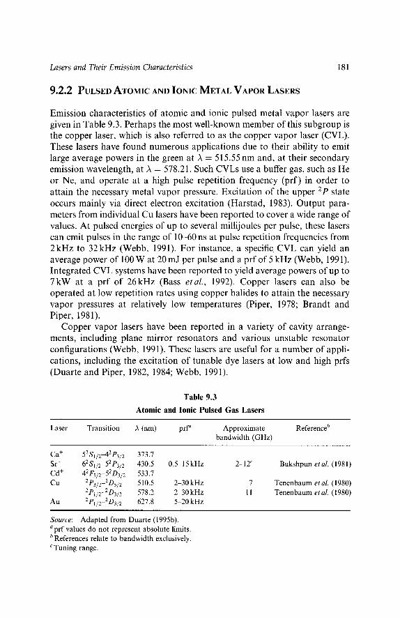
Lasers and Their Emission Characteristics 181
9 .2 .2 PULSED ATOMIC AND IONIC METAL VAPOR LASERS
Emission characteristics of atomic and ionic pulsed metal vapor lasers are given in Table 9.3. Perhaps the most well-known member of this subgroup is the copper laser, which is also referred to as the copper vapor laser (CVL). These lasers have found numerous applications due to their ability to emit large average powers in the green at A - 515.55 nm and, at their secondary emission wavelength, at A = 578.21. Such CVLs use a buffer gas, such as He or Ne, and operate at a high pulse repetition frequency (prf) in order to attain the necessary metal vapor pressure. Excitation of the upper 2p state occurs mainly via direct electron excitation (Harstad, 1983). Output para- meters from individual Cu lasers have been reported to cover a wide range of values. At pulsed energies of up to several millijoules per pulse, these lasers can emit pulses in the range of 10-60 ns at pulse repetition frequencies from 2kHz to 32kHz (Webb, 1991). For instance, a specific CVL can yield an average power of 100 W at 20 mJ per pulse and a prf of 5 kHz (Webb, 1991). Integrated CVL systems have been reported to yield average powers of up to 7kW at a prf of 26kHz (Bass etal . , 1992). Copper lasers can also be operated at low repetition rates using copper halides to attain the necessary vapor pressures at relatively low temperatures (Piper, 1978; Brandt and Piper, 1981).
Copper vapor lasers have been reported in a variety of cavity arrange- ments, including plane mirror resonators and various unstable resonator configurations (Webb, 1991). These lasers are useful for a number of appli- cations, including the excitation of tunable dye lasers at low and high prfs (Duarte and Piper, 1982, 1984; Webb, 1991).
Table 9.3
Atomic and Ionic Pulsed Gas Lasers
Laser Transition A (nm) p r f f Approximate Reference b bandwidth (GHz)
Ca + 52S1/2-42P3/2 373.7 Sr + 62S1/2-52P3/2 430.5 0.5-15kHz Cd + 42Fs/z-52D3/2 533.7 Cu 2P3/z-205/2 510.5 2-30 kHz
2P1/2-2D3/2 578.2 2-30 kHz Au 2P1/2-2D3/2 627.8 5-20 kHz
2-12 c Bukshpun et al. ( 1981)
7 Tenenbaum et al. (1980) 11 Tenenbaum etal. (1980)
Source: Adapted from Duarte (1995b). a prf values do not represent absolute limits. 6 References relate to bandwidth exclusively. c Tuning range.

182 Tunable Laser Optics
9.2.3 CONTINUOUS-WAVE GAS LASERS
Perhaps the most well-known gas laser is the helium-neon (He-Ne) laser. Its most most well-known line corresponds to the 3s2-2p4 transition at A -- 632.82 nm. This transition is made possible by excitation transfer from atoms at the helium metastable level He*(23S1) to ground state Ne atoms (Willett, 1974). The emission from this laser is characterized by a most beautiful TEM00 beam at a laser linewidth typically less than a few gigahertz in the absence of frequency-selective intracavity optics. At the referred wavelength, and depending on the discharge length, available powers vary from a few milliwatts to a few tens of milliwatts. Additional transitions available from the He-Ne laser are listed in Table 9.4. He-Ne lasers incor- porating broadband mirrors and tuning optics can emit at several visible transitions.
Another CW gas laser that is widely used in the laboratory, due to its powerful blue-green transitions, is the Ar + laser. All the transitions listed in Table 9.5 are excited via electron impact (Willett, 1974). The dominant CW transitions are those at 487.99nm and 514.53nm. It should be noted that relatively compact Ar + lasers can be engineered to deliver powers at a range of tens of milliwatts, while large systems have been configured to yield as much as 175 W (Anliker et al., 1977). An additional feature of laboratory Ar + lasers is the option to tune from line to line using intracavity optics.
Additional CW metal vapor lasers are the He-Zn and the He-Cd lasers. Ion transitions in these lasers are excited via Penning and Duffendack
Table 9.4
Transitions of Continuous-Wave He-N e Laser a
Transition b A (nm) ~
3s2-2p10 543.30 3s2-2p8 593.93 3s2-2p7 604.61 3s2-2p6 611.80 3s2-2p4 632.82 2sa-2p8 1,114.30 2s2-2p4 1,152.35 2sa-2p3 1,268.90 2s2-2pl 1,523.10
a Partial list of available transitions. b Transition assignment following Willett (1974). CWavelength values from Beck etal. (1976).

Lasers and Their Emiss ion Characteristics 183
Table 9.5
Ionized Continuous-Wave Gas Lasers a
Laser Transition b A (nmy
Ar + 4p2 P{. 4p2S 4,02/~ 4pZD( 4p2 P~. 4paD~ 4p2D~
4p2D~
4pqS! 4p4DI
,2-4s2P3/2 ,2-4s2P1/2 ,2-4s2P3/2 ,2-4s2P3/2 ,2-4s2P1/2 ,2-4s2P3/2 ,2-4s2P1/2 ~-4dZ D3/2 ,2-4s2P3/2 ,2-4s2P1/2
Zn + 4f21~5/2-4d2D3/2 4f 2 F~ /2--4d2 05/2
4s22 D 3) 2-4p 2 P~I/2 4s22 O5/2-4p2 P~3}2
5P 2 P~3/2 -5S2 S1/2
Kr + 4p4P~3/2-5s4P3/2 5p4 P~5 /2-5s4 P3 /2 5P 4D0/2 -5s2P3/2 5P 4 P~5/2 -5S2 P3/2 5P 4 P~3/2 -5S2 P1/~
5p4P~3/2-4d2D1/2
Cd+ 5s22 D5/2-5p 2 P~3/2 2 0 2 - 4f F~/z-5dAD3/2
4f Z F7/z-5dZ D5/2 6g 2 G7/2-4f 2 F~ 6gZ G9 /z-4 f Z F~ /2 Of 2 F~/z-6d 2 D3/2 6f 2 F~ /z-6d 2 D5/2 6P 2 P~3/2 -6S2 S1/2 6pZ P~l }z-6sZ SI /2 9s 2 S1/' 2-7p 2 P~3/2
I + 6p'3 Dz-6J 3 D o 6p' 3 F2-6J 3 D2 6p '3 D2-6J 3 D O 6p'3 D1-6s' 3 D O 6pt 3 D1-6d 3 D O 6p'3F2-5d'3D o 6p'3D2-5d'3D o 6p'3F2-5d'3D o 6p~3Di-5dt3D 0 6pt 3 D2-5dt 3 F~3 6p~3F2-5dt3F3
a Partial list of available transitions. b Transition assignment following Willett (1974). CWavelength values from Beck etal. (1976).
454.50 457.93 465.79 472.69 476.49 487.99 496.51 510.72 514.53 528.69
491.16 492.40 589.44 747.88 758.85
520.83 530.87 568.19 647.09 752.55 799.32
441.56 533.75 537.80 635.48 636.00 723.70 728.40 806.70 853.00 887.80
540.73 567.81 576.07 612.75 658.52 703.30 713.89 761.85 773.57 817.01 880.43

184 Tunable Laser Optics
reactions (Piper and Gill, 1975). In the first reaction the helium metastable He*(3S1) interacts with the metal atoms, in the second reaction it is the helium ion He+(2S1/2) that participates in the excitation. In the case of the He-Zn laser, the transitions at 491.16nm, 492.40nm, and 758.85nm are excited via Duffendack reactions, which can occur only in hollow-cathode discharges that give origin to energetic electrons. Using a hollow-cathode He-CdI2 discharge, Piper (1976) combined simultaneously four transitions from Cd + and 11 transitions from I + to produce a most striking TEM00 white-light laser beam. All of the I + transitions listed in Table 9.5 partici- pated in the emission, plus the Cd + transitions at 441.56nm, 533.75nm, 537.80nm, and 806.70nm. All of these transitions are excited via Duffen- dack reactions, except the 441.56 nm transition from Cd + which results from Penning ionization.
For a survey of CW CO2 lasers, the reader should refer to Willett (1974) and Freed (1995). An excellent review on frequency selectivity in CO2 lasers is provided by Tratt et al. (1985).
9.3 DYE LASERS
Dye lasers are inherently tunable and well suited for the generation of high- average powers (Duarte, 1991 a). These lasers can be divided into two main categories: pulsed dye lasers and CW dye lasers. These lasers, using various dyes, can span the electromagnetic spectrum, from the near-ultraviolet to the near-infrared. Some individual dyes, such as rhodamine 6G, can provide tuning ranges in excess of 50nm. The appendix at the end of the book contains a fairly comprehensive listing of well-known laser dyes, including molecular weight, molecular structure, and approximate tuning ranges. For historical reviews the reader should refer to SchS.fer (1990) or Duarte and Hillman (1990).
9.3.1 PULSED DYE LASERS
Pulsed dye lasers are divided into two subclasses: laser-pumped pulsed dye lasers and flashlamp-pumped pulsed dye lasers.
As is apparent from Table 9.6, laser-pumped dye lasers can provide either hundreds of joules per pulse at low repetition rates or very high average powers, well into the kilowatt regime at prfs in excess of 10 kHz. Excellent reviews on CVL-pumped dye lasers are given by Webb (1991) and on excimer-laser-pumped dye lasers by Tallman and Tennant (1991).

Lasers and Their Emission Characteristics
Table 9.6
Performance of High-Power Laser-Pumped Dye Lasers
185
Excitation Pulse laser energy
prf Average Efficiency Dye power (%)
Reference
XeC1 800 ja Very low XeC1 200 mJ 250 Hz
CVL >190 mJ 13.2 kHz
27 50 W 20
>2.5kW >50
Coumarin 480 Tang etal. (1987) TBS Tallman and
Tennant (1991) Rhodamine b Bass et al. (1992)
Source: Adapted from Duarte (1995b). a Pulse length quoted at 500 ns. bTuning range: 550-650nm (Bass etal., 1992).
The performance of laboratory-size laser-pumped dye lasers can be illus- trated by considering the work of Bos (1981), who reported a linewidth of Au ~ 320MHz at 590nm with a telescopic oscillator incorporating an intracavity etalon. Using three stages of amplification, the output energy was 165mJ at overall conversion efficiency of 55% for excitation at 532nm. Employing an HMPGI grating oscillator and two stages of amplification, Dupre (1987) reported 3.5 mJ and Au = 1.2 GHz at 440 nm. The conversion energy efficiency was ~9% for excitation at 355 nm.
Copper Vapor Laser excitation of an HMPGI grating oscillator yielded Au ~ 600MHz for A = 575nm, and pulse lengths of 12ns (FWHM) at conversion efficiencies of ~5% (Duarte and Piper, 1984). The average out- put power was 80 mW at a prf of 8 kHz. Using the same class of multiple- prism oscillator and one amplifier stage, Singh eta l . (1994) reported Au ~ 1.5 GHz and a conversion efficiency of 40% at a prf of 6.5 kHz.
The performance of large flashlamp-pumped dye lasers is summarized in Table 9.7. For a comprehensive review of flashlamp-pumped dye lasers, the reader should consult Everett (1991). In general, these lasers have been used to generate large energies in pulses in the microsecond regime. The energy per pulse is such that fairly modest prfs can generate average powers in the kilowatt regime.
Besides their intrinsic ability to generate large pulsed energies, flashlamp- pumped dye lasers have been configured in small-scale laboratory versions designed to yield fairly narrow-linewidth tunable laser emission. For a review on this subject, see Duarte (1995b).
A ruggedized MPL grating coaxial flashlamp-pumped dye laser oscillator yielding Au ~ 375 MHz at amplified spontaneous emission levels a few parts in 10 -7 was reported by Duarte etal . (1991). This dispersive oscillator provided ~3 mJ per pulse using rhodamine 590 at a concentration of 0.01 mM.

186 Tunable Laser Optics
Table 9.7
Performance of High-Energy Flashlamp-Pumped Dye Lasers
Excitation Pulse Output Efficiency Dye duration energy (%)
Reference
Linear a 7 las 40 J 0.4 Rhodamine 6G at 0.08 mM
Transverse b 5 las 140 Jr 1.8 Rhodamine 6G at 0.025 mM
Coaxial 10 las 400 J 0.8 Rhodamine 6G at 0.022 mM
Fort and Moulin (1987) Klimek et al. (1992) Baltakov et al. (1974)
Source: Adapted from Duarte (1995b). a Employs 12 flashlamps in a linear configuration. b Employs 16 flashlamps in a transverse configuration. C yields an average power of 1.4 kW at a prf of 10 Hz.
The output from narrow-linewidth oscillators can be amplified using single-stage amplifiers to yield hundreds of millijoules per pulse. Flamant and Maillard (1984) used a two-etalon oscillator to excite a flat-mirror amplifier to attain Au = 346 MHz and a pulse energy of 300 mJ at 590 nm. Using a multiple-prism grating oscillator and a single-stage unstable- resonator amplifier, Duarte and Conrad (1987) achieved Au ~ 375 MHz and a pulse energy of 600mJ at 590 nm.
In addition to traditional liquid dye lasers there has been considerable research and development activity in the area of solid-state dye lasers. An excellent review on dye-doped solid-state matrices is provided by Costela e ta l . (1998), and the photophysical properties of these solid-state gain materials have been characterized by Holzer et al. (2000). Although most recent activity has been centered on polymeric matrices and hybrid silicate- polymer composite materials, there has also been work reported on crystal- line dye lasers (Rifani et al., 1995; Braun et al., 2000). A review of organic lasers, including solid-state dye lasers, aimed at assessing the development of electrically pumped polymer lasers is given by Kranzelbinder and Leising (2000). Work at establishing quasi-CW oscillation using improved hybrid dye-doped polymer-nanoparticle matrices is also in progress.
The performance of broadband solid-state dye lasers is summarized in Table 9.8. Optimized multiple-prism grating solid-state oscillators, as described in Chapter 7, have yielded tuning ranges in the range of 550-603 nm with TEM00 laser beams, at beam divergences ~1.5 times the diffraction limit. The emission is in a single longitudinal mode at Au ~ 350 MHz in pulses ~3 ns (FWHM) with a near-Gaussian temporal profile. Conversion efficiency is reported at ~5%, and the ASE levels are extremely low at ,-,~10 -6

Lasers and Their Emis s ion Characteris t ics
Table 9.8
Performance of Broadband Solid-State Dye Lasers
Excitation Matrix Dye Output Efficiency source energy (%)
Reference
187
Flashlamp PMMA a Rhodamine 590 50 mJ at 0.11 mM
Nd:YAG MPMMA b Rhodamine 65 laser (2u) 11B at 0.5 mM LPDL c HEMA:MMA d Rhodamine 6G 0.8 mJ 40
at 0.5 mM FLPDL e TEOS c Rhodamine 6G 2.5 mJ
at 2 mM Nd:YAG ORMOSIL g Rhodamine 6G 3.5mJ 35 laser (2u) at 0.086 mM
Pacheco et al. (1988)
Maslyukov et al. (1995)
Duarte et al. (1997)
Duarte et al. (1993)
Larrue et al. (1994)
Source: Adapted from Duarte (1995b). a Polymethyl methacrylate. b Modified Polymethyl metracrylate. c Laser-pumped dye laser using Coumarin 152. d2_hydroxyethyl methacrylate:methyl methacrylate e Flashlamp-pumped dye laser using Coumarin 525. fSi(OC2H5)4 g Organically modified silicate.
(Duarte, 1999). Transverse excitation in the long-pulse regime of a four-prism grating solid-state dye laser oscillator has led to pulses as long as 105 ns (FWHM) and Au ~ 650 MHz at pulsed energies of ~0.4 mJ (Duarte et al., 1998).
9.3.2 CONTINUOUS-~AVE DYw LASERS
Dye lasers have had a significant impact in high-resolution spectroscopy and other applications, including laser cooling, given their tunability, excellent TEM00 beam quality, and intrinsic narrow linewidths, which can readily reach a level of a few megahertz. Continuous-wave dye lasers typically use Ar + and Kr + as excitation sources, although in principle they could use any compatible laser yielding TEM00 emission. It should be noted that CW dye lasers have been excited with a variety of lasers, including diode lasers (see, for example, Scheps, 1993). Table 9.9 summarizes the performance of rela- tively high-power dye lasers, some of which yield SLM oscillation at line- widths in the megahartz regime. Stabilization techniques can produce significant improvements in laser linewidth, as indicated in Table 9.10. Here,

188 Tunable Laser Optics
Table 9.9
Performance of High-Power CW Dye Lasers
Cavity Spectral range Linewidth Output Efficiency (%) Reference (nm) power
Linear a 33 W b'~ 30 Anliker etal. (1977) Linear a 560-650 SLM d 33 W ef 17 Baving et al. (1982) Ring a 407-887 g SLM a 5.6W h 23.3 Johnston etal. (1982)
Source: Adapted from Duarte (1995b). a Under Ar + laser excitation. b Maximun CW power quoted: 52 W for a pump power of 175 W. e Using Rhodamine 6G at 0.7 mM. a Linewidth values can be in the few MHz range. eWithout intracavity tuning prism, quoted output power is 43 W for a pump power of 200 W. fUsing Rhodamine 6G at 0.94mM. g Using 11 dyes. h Using Rhodamine 6G.
the use o f an r f -opt ica l h e t e r o d y n e lock t echn ique enab led D r e v e r et al.
(1983) to reach a laser l inewid th of 100 Hz. A n excel lent review on C W dye
lasers is given by H o l l b e r g (1990).
A fu r the r t ower ing c o n t r i b u t i o n of the C W dye lasers to the field of opt ics
a n d lasers was their use as tools in the d e v e l o p m e n t of u l t r a s h o r t - p u l s e lasers t h a t gave or ig in to the f e m t o s e c o n d lasers. A m o n g the i m p o r t a n t concep t s
deve loped in this e n d e a v o r were the g e n e r a t i o n of b a n d w i t h - l i m i t e d u l t ra-
sho r t pulses ( R u d d o c k a n d Bradley , 1976), the co l l id ing-pulse m o d e ( C P M )
lock ing t echn ique ( F o r k e ta l . , 1981), and p r i sma t i c pulse c o m p r e s s i o n
(Diete l et al., 1983; F o r k et al., 1984). Us ing an ex t racav i ty pulse c o m p r e s s o r ,
Table 9.10
Performance of Frequency-Stabilized CW Dye Lasers a
Stabilization method Linewidth Frequency drift Reference
Cavity side lock a 150 kHz a 50 MHz/h Divens and Jarrett (1982) rf-optical 100 Hz Drever etal. (1983) Heterodyne lock b <750 Hz a 720 Hz/s Hough et al. (1984) Post laser e 20 kHz d Hall and H~nsch (1984)
a Uses two Fabry-Perot interferometers. b Uses a reference cavity. C Uses acousto-optic and electro-optic modulators. For dye lasers with intrinsic linewidths of ~1MHz, this method has yielded ultimate linewidths of ~1 kHz (Hollberg, 1990). a Emission source: ring dye laser.

Lasers and Their Emission Characteristics 189
consisting of a four-grating array and a four-prism array, Fork et al. (1987) compressed a 50-fs pulse further to just 6 fs. Diels (1990) and Diels and Rudolph (1996) provide comprehensive reviews on this subject.
9.4 S O L I D - S T A T E L A S E R S
The solid-state laser field is vast and includes traditional crystalline materials and fiber gain media. These lasers can emit in both the pulsed and the CW regimes. In this section some of the most well-known gain media are surveyed, with emphases on spectral characteristics.
9.4.1 IONIC SOLID-STATE LASERS
Optically pumped ionic solid-state lasers include the well-known Nd laser, which can exist in either a crystalline or a glass host. These lasers are very well suited to be configured in various cavity arrangements, including unstable resonator arrangements, which yield single-transverse-mode emission. The linewidth of a TEM00 laser at 1064 nm is typically 15-30 GHz (Chesler and Geusic, 1972). Frequency doubling using nonlinear crystals, intracavity or extracavity, yields efficient conversion into the visible. Originally, these lasers were excited using flashlamp pumping; however, diode laser pumping has become rather pervasive. Commercially available diode-laser pumped Nd:YAG lasers can yield tens of watts at prfs in the kilohertz regime. Individual laser pulse lengths can be in the range of 10-15 ns. Ionic gain media in crystalline hosts has also lased in the CW regime.
Nd:glass lasers are operated mainly at very high peak powers and low prfs in the TW regime. Some of the most well-known ionic solid-state lasers are listed in Table 9.11, along with their respective transitions.
9.4.2 TRANSITION METAL SOLID-STATE LASERS
Transition metal solid-state lasers include the alexandrite and the Ti:sap- phire lasers, which are widely tunable. This quality has made the Ti:sapphire laser particularly applicable to the generation of ultrashort pulses in the femtosecond regime. Although the ruby laser is operated mainly in the pulsed regime, typically delivering a few joules of energy per pulse, the other two media are very versatile and are well suited to both pulsed and CW operation (Walling and Peterson, 1980; Walling etal. , 1980a; Moulton,

190
Table 9.11
Ionic Solid-State Lasers
Ion Transition A (nm)
Yb 3+ 2Fs/2-2F7/2 1015 a Nd3+ 4 F3/2 __4 I11/2 10646
2u 532 3u 355 4u 266
E r 3 + 4113/2_4115/2 1540 a Tm 3+ 3H4-3H 6 2013 c Ho 3+ 517-518 2097 c
Source: Adapted from Duarte (1995b). a In glass host. bin YAG host. c In Y3AlsO12 host.
Tunable Laser Optics
1986). Tuning ranges are listed in Table 9.12. A comprehensive review of t ransi t ion metal solid-state lasers has been given by Barnes (1995a).
All solid-state Ti:sapphire lasers are available commercial ly with TEM00 beam profiles and emission in the s ingle- longi tudinal-mode domain , deliver- ing average powers in the watts regime at ~10 kHz. Using CVL pumping, nar row-l inewidth emission has been demons t ra ted at average powers of 5 W at 6.2 kHz, at a conversion efficiency of ~ 2 6 % (Cout ts et al., 1998). Liquid- n i t rogen cooling of Ti :sapphire gain media has resulted in C W ou tpu t powers of up to 43 W at an efficiency of ~ 4 2 % for b r o a d b a n d lasing (Erbert et al., 1991). In the ul t rashor t -pulse regime, Ti:sapphire lasers have been shown to deliver pulses as short as 5 fs (Ell et al., 2001).
Table 9.12
Transition Metal Solid-State Lasers
Laser Ion:host crystal Transition A (nm)
Ruby Cr 3+ :A12 03 2E(E)_4A2 694.3 Emerald Cr 3+ :Be3 A12(SIO3)6 4 T2_4 A2 695-835 a Alexandrite Cr 3+ :BeAI2 04 4 T2_4A2 701-818 b
Ti:sapphire Ti 3+ :A1203 2 T2_2 E 660-986 c
a Gain range in the pulsed regime (Shand and Walling, 1982). b Tuning range in the pulsed regime (Walling et al., 1980b). CTuning range in the pulsed regime (Moulton, 1986).
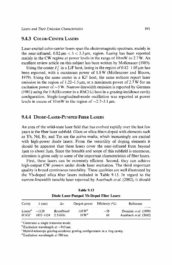
Lasers and Their Emission Characteristics 191
9.4.3 COLOR-CENTER LASERS
Laser-excited color-center lasers span the electromagnetic spectrum, mainly in the near-infrared, 0.82 gm < A < 3.3 lam, region. Lasing has been reported mainly in the CW regime at power levels in the range of 10 mW to 2.7 W. An excellent review article on this subject has been written by Mollenauer (1985).
Using the center F f in a LiF host, lasing in the region of 0.82-1.05 gm has been reported, with a maximum power of 1.8 W (Mollenauer and Bloom, 1979). Using the same center in a KF host, the same authors report laser emission in the region of 1.22-1.5 lam, at a maximum power of 2.7 W for an excitation power of ~5 W. Narrow-linewidth emission is reported by German (1981) using the FA(II) center in a RbCI:Li host in a grazing-incidence cavity configuration. Single-longitudinal-mode oscillation was reported at power levels in excess of 10 mW in the region of ~2.7-3.1 gm.
9.4.4 DIODE-LASER-PUMPED FIBER LASERS
An area of the solid-state laser field that has evolved rapidly over the last few years is the fiber laser subfield. Glass or silica fibers doped with elements such as Yb, Nd, Er, and Tm are the active media, which increasingly are excited with high-power diode lasers. From the versatility of doping elements it should be apparent that these lasers cover the near-infrared from beyond 1 gm to about 3gm. Since the breadth and scope of this subfield is enormous, attention is given only to some of the important characteristics of fiber lasers.
First, these lasers can be extremely efficient. Second, they can achieve high-output CW powers under diode laser excitation. The third important quality is broad continuous tunability. These qualities are well illustrated by the Yb-doped silica fiber lasers included in Table 9.13. In regard to the narrow-linewidth tunable laser reported by Auerbach et al. (2002), it should
Table 9.13
Diode-Laser-Pumped Yb-Doped Fiber Lasers
Cavity A (nm) Au Output power Efficiency (%) Reference
Linear a ~ 1 1 2 0 Broadband ll0W b ~58 Dominic etal. (1999) HTGI c 1032-1124 2.5 GHz 10W a 68 Auerbach etal. (2002)
a Generates a single transvese mode. b Excitation wavelength at ~915 nm. c Hybrid-telescope grazing-incidence grating configuration in a ring cavity. d Excitation wavelength at 980 nm.

192 Tunable Laser Optics
be mentioned that the authors report extremely low levels of ASE. Also, the hybrid-telescope-grazing-incidence (HTGI) grating configuration (Yodh e t a l . , 1984; Smith and DiMauro, 1987) used to induce narrow-linewidth oscillation is a variant of the principle of the HMPGI grating configurations (Duarte and Piper, 1981, 1984) described in Chapter 7. Both lasers listed in Table 9.13 were excited with diode lasers. The 110-W laser used four laser diode bars providing a combined power of ~180 W.
9.4.5 OPTICAL PARAMETRIC OSCILLATORS
Although the optical parametric oscillator (OPO) does not involve the process of population inversion in its excitation mechanism, it is included here because it is a source of spatially and spectrally coherent emission, which is inherently tunable. For detailed review articles on this subject, the reader is referred to Barnes (1995b) and Orr et al. (1995). Spectral character- istics of several well-known OPOs are given in Table 9.14.
Optical parametric oscillators are optically pumped devices that make wide use of Nd:YAG lasers and the different harmonics that can be provided with these excitation sources. A fairly instructive case study on the perform- ance of pulsed OPOs is provided by Schr6der e t a l . (1994), who report an output energy of 77mJ for an excitation energy of 170mJ at 355 nm for a 15-mm-long LiB3Os crystal. The emission bandwidth was ~0.5 nm (~366 GHz) at A ~ 640 nm. This performance was obtained using excitation pulses 5-6 ns in duration at a prf of 10 Hz. Pulsed OPOs for analytical applications tend to operate at prfs of ~10 Hz (He and Orr, 2001). Barnes and Williams-Byrd (1995) discuss thermally induced phase mismatch and thermally induced lensing that tend to limit the average power in OPOs and optical parametric amplifiers.
Table 9.14
Pulsed Optical Parametric Oscillators
Crystal Optical transmission (l.tm) a Ap (nm) Tuning range ( g m ) Reference
KTP 0.35-4.5 532 0.61-4.0 Orr etal. (1995) BBO 0.20-2.2 355 0.41-3.0 Orr et al. (1995) LBO 0.16-2.3 355 0.41-2.47 Schr6der et al. (1994) LiNbO3 0.33-5.5 532 0.61-4.4 Orr et al. (1995) AgGaS2 0.15-13 1064 1.4-4.0 Fan et al. (1984)
aFor the ordinary ray (Barnes, 1995b).

Lasers and Their Emission Characteristics 193
Certainly, all the linewidth-narrowing techniques described in Chapter 7 are applicable to OPOs, further details are given in Chapter 8. For example, a multiple-prism grating cavity incorporating an intracavity etalon, in a L i N b O 3 0 P O yielded a linewidth of ~30MHz at a wavelength of ~3.4 lam. The energy conversion efficiency was reported at ~0.74%.
Initially, OPOs in the continuous-wave regime were longitudinally excited by CW frequency-doubled Nd:YAG lasers (Smith et al., 1968). An improved approach consists of using diode-laser excitation in intracavity configura- tions. Using fiber-coupled excitation from a diode laser at 940 nm, Jensen etal . (2002) excited a Yb:YAG crystal whose emission was focused on a periodically poled LiNbO3 (PPLN) crystal. For a diode laser power of 13.5W, tunable emission in the range of 3.82-4.571am was reported at output powers of 200 mW (Jensen et al., 2002).
Femtosecond OPOs in linear and ring cavities incorporating multiple- prism pulse compressors have been discussed by Powers et al. (1993).
9.5 S E M I C O N D U C T O R L A S E R S
The area of semiconductor lasers is a rapidly evolving field that can be classified into high-power lasers, external-cavity lasers, and miniature lasers. Semiconductor lasers work via direct electrical excitation, are compact, offer wavelength tunability, and can be very stable. The tuning ranges available from various semiconductor laser materials are listed in Table 9.15. Their compactness, with aperture dimensions in the micrometer regime, results in large beam divergences that require external or intracavity beam-shaping optics to reduce the divergence.
Table 9.15
Wavelength Coverage of Semiconductor Laser Materials
Semiconductor Wavelength coverage (nm)
II-VI materials Blue-green A1GaInP/GaAs 610-690 A1GaAs/GaAs 780-880 InGaAs/GaAs 880-1100 InGaAsP/InP 1100-1600 InGaAs/InP 1600-2100
Source: From Zorabedian (1995).

194 Tunable Laser Opt ics
High-power diode lasers, such as those used in the excitation of crystalline solid-state lasers and fiber lasers, integrate many individual diode lasers to increase the overall output power. Arrays of many diode lasers in parallel form what is known as a "bars." The divergent emission from these bars is collected and guided using external beam-shaping optics. As indicated in Table 9.16, these bars can yield powers in the range of 10-40 W. For uses requiring even higher output powers, such as industrial applications, the bars are further integrated into "stacks." These stacks can yield powers in the kilowatt regime.
One area of research that has received considerable attention is the line- narrowing and tunability of semiconductor devices. External-cavity tunable semiconductor lasers utilize grating and multiple-prism grating cavity archi- tectures similar to those described in Chapter 7. The performance of these lasers, which have been widely applied in areas such as laser cooling and Bose-Einstein condensation (BEC), is summarized in Table 9.17. Note that although many authors for convenience use open-cavity configurations, only closed-cavity configurations are considered here, given their superior signal-to-noise characteristics (Zorabedian, 1992). For reviews on this sub- ject, the reader is referred to Zorabedian (1995), Duarte (1995c), and Fox et al. (1997).
Table 9.16
Performance of CW Diode-Laser Arrays
A (nm) Output power (W) Reference
791 10 Srinivasan et al. (1999) ~915 45 Dominic et al. (1999) 980 29 Auerbach et al. (2002)
Semiconductor
Table 9.17
External-Cavity Tunable Semiconductor Lasers a
Cavity Tuning Au Output power range (nm)
Reference
InGaAsP/InP LG b 1285-1320 31 kHz 1 mW InGaAsP/InP MPL 1255-1335 100 kHz GaA1As LG b 815-825 1.5 MHz 5 mW
Shan et al. (1991) Zorabedian (1992) Fleeming and Mooradian (1981)
a All entries in this table use closed-cavity configurations. b Tuning is performed by a Littrow grating (LG).

Lasers and Their Emission Characteristics 195
One further variant in the field of tunable semiconductor lasers consists of building miniature lasers for applications in optics communications. One such approach utilizes a silicon microelectromechanical system (MEMS) grazing-incidence grating external cavity (Berger et al., 2001). This miniature dispersive laser has been shown to yield narrow-linewidth emission tunable for over a 26-nm range in the near infrared. A second approach tunes an integrated vertical-cavity surface-emitting laser (VCSEL) that varies its wavelength by changing the length of the cavity (Kner et al., 2002). The length of the cavity is changed by displacing the voltage-driven output mirror. The performance of these lasers is summarized in Table 9.18.
9.6 A D D I T I O N A L L A S E R S
An important source of widely tunable coherent radiation not already included in this survey is the free-electron laser (FEL). The reason for this choice is that FELs are fairly large high-power devices that require accel- erator technology. In his review of FELs, Benson (1995) reports that various devices around the world cover, with their primary emission wavelengths, the electromagnetic spectrum from 2 ~tm to 2500 ~tm. An excellent book on FELs was written by Brau (1990).
Additional lasers not included in this survey are chemical lasers, far- infrared lasers, and nuclear-pumped lasers. Chemical lasers are large and powerful sources of coherent radiation suitable for military applications. The HF laser that results from a reaction between H2 and F emits in the region of 2.640-2.954 lam (Miller, 1988). The iodine laser, which originates from a reaction of oxygen and iodine, emits at 1.3 ~tm (Yoshida et al., 1988).
Table 9.18
Miniature Tunable Semiconductor Lasers
Semiconductor Cavity Tuning Av Output Reference range (nm) power
InGaAsP/InP GIG a 1531.5-1557.9 2MHz 20mW Berger eta1. (2001) GaAs/A1GaAs b Mirror c 1533-1555 SM d 0.9mW Kner etal. (2002)
a Uses a silicon MEMS-driven grazing-incidence grating cavity. bVCEL C Tuning is achieved by displacing a voltage-driven micromirror that is supported by a cantilever. dQuoted as single mode.

196 Tunable Laser Optics
Far-infrared lasers are optically pumped molecular lasers that cover the spectrum deep in the infrared from 0.1 to 1 mm (see, for example, James et al., 1988). The active media in these lasers are molecules such as HCOOH and CH3OH (Farhoomand and Pickett, 1988), and the excitation is pro- vided by CO2 lasers.
Nuclear-pumped lasers use reactors as excitation source and various gaseous mixtures as the lasing media (Schneider and Cox, 1988).
R E F E R E N C E S
Anliker, P., Luthi, H. R., Seelig, W. Steinger, J., Weber, H. P., Leutwyler, S., Schumacher, E., and Woste, L. (1977). 33-W CW dye laser. IEEE J. Quantum Electron. QE-13, 547-548.
Auerbach, M., Adel, P., Wandt, D., Fallnich, C., Unger, S., Jetschke, S., and Mller, H.-R. (2002). Opt. Express 10, 139-144.
Baltakov, F. N., Barikhin, B. A., and Sukhanov, L. V. (1974). 400-J pulsed laser using a solution of rhodamine-6G in ethanol. JETP Lett. 19, 174-175.
Barnes, N. P. (1995a). Transition metal solid-state lasers. In Tunable Lasers Handbook (Duarte, F. J., ed.). Academic Press, New York, pp. 219-291.
Barnes (1995b). Optical parametric oscillators. In Tunable Lasers Handbook (Duarte, F. J., ed.). Academic Press, New York, pp. 293-348.
Barnes, N. P., and Williams-Byrd, J. A. (1995). Average power effects in parametric oscillators and amplifiers. J. Opt. Soc. Am. B 12, 124-131.
Baving, H. J., Muuss, H., and Skolaut, W. (1982). Appl. Phys. B. 29, 19-21. Bass, I. L., Bonanno, R. E., Hackel, R. H., and Hammond, P. R. (1992). High-average-power
dye laser at Lawrence Livermore National Laboratory. Appl. Opt. 31, 6993-7006. Beck, R., Englisch, W., and Gfirs, K. (1976). Table of Laser Lines in Gases and Vapors. Springer-
Verlag, Berlin. Benson, S. V. (1995). Tunable free-electron lasers. In Tunable Lasers Handbook (Duarte, F. J.,
ed.). Academic Press, New York, pp. 167-218. Berger, J. D., Zhang, Y., Grade, J. D., Howard, L., Hrynia, S., Jerman, H., Fennema, A.,
Tselikov, A., and Anthon, D. (2001). External cavity diode lasers tuned with silicon MEMS. IEEE LEOS Newslett. 15(5), 9-10.
Bobrovskii, A. N., Branitskii, A. V., Zurin, M. V., Koshevnikov, A. V., Mishchenko, V. A., and Myl'nikov, G. D. (1987). Continuously tunable TEA CO2 laser. Sov. J. Quantum Electron. 17, 1157-1159.
Bos, F. (1981). Versatile high-power single-longitudinal-mode pulsed dye laser. Appl. Opt. 20, 1886-1890.
Bradley, C. C., McClelland, J. J., Anderson, W. R., and Celotta, R. J. (2000). Magneto-optical trapping of chromium atoms. Phys. Rev. 61, 053407.
Brandt, M., and Piper, J. A. (1981). Operating characteristics of TE copper bromide lasers. IEEE J. Quantum Electron. QE-17, 1107-1115.
Brau, C. A. (1990). Free-Electron Lasers. Academic Press, New York. Braun, I., Ihlein, G., Laeri, F., N6ckel, J. U., Schulz-Ekloff, G., Schfith, F., Vietze, U., Weiss, O.,
and W6hrle, D. (2000). Hexagonal microlasers based on organic dyes in nanoporous crystals. Appl. Phys. "70, 335-343.
Broyer, M., Chevaleyre, J., Delacr6taz, G., and W6ste, L. (1984). CVL-pumped dye laser spectroscopic application. Appl. Phys. B. 35, 31-36.
Lasers and Their Emission Characteristics 197
Buffa, R., Burlamacchi, P., Salimbeni, R., and Matera, M. (1983). Efficient spectral narrowing of a XeC1 TEA laser. J. Phys. D: Appl. Phys. 16, L125-L128.
Bukshpun, L. M., Zhukov, V. V., Latush, E. L., and Sem, M. F. (1981). Frequency tuning and self-locking in He-Sr recombination laser, Sov. J. Quantum Electron. 11, 804-805.
Caro, R. G., Gower, M. C., and Webb, C. E. (1982). A simple tunable KrF laser system with narrow bandwidth and diffraction-limited divergence. J. Phys. D." Appl. Phys. lfi, 767-773.
Chesler, R. B., and Geusic, J. E. (1972). Solid-state ionic lasers. In Laser Handbook, Vol. 1 (Arecchi, F. T., and Schulz-Dubois, E. O., eds.). North Holland, Amsterdam, pp. 325-368.
Costela, A., Garcia-Moreno, I., Figuera, J. M., Amat-Guerri, F., and Sastre, R. (1998). Poly- meric matrices for lasing dyes: recent developments. Laser Chem. 18, 63-84.
Coutts, D. W., Wadsworth, W. J., and Webb, C. E. (1998). High-average-power blue generation from a copper-vapor laser-pumped titanium sapphire laser. J. Mod. Opt. 45, 1185-1197.
Diels, J.-C. (1990). Femtosecond dye lasers. In Dye Laser Principles (Duarte, F. J., and Hillman, L. W., eds.). Academic Press, New York, pp. 41-132.
Diels, J.-C., and Rudolph, W. (1996). Ultrashort Laser Pulse Phenomena. Academic Press, New York.
Dietel, W., Fontaine, J. J., and Diels, J.-C. (1983). Intracavity pulse compression with glass: a new method of generating pulses shorter than 60 fs. Opt. Lett. 8, 4-6.
Divens, W. G., and Jarrett, S. M. (1982). Rev. Sci. Instrum. 53, 1363. Dominic, V., MacCormack, S., Waarts, R., Sanders, S., Bicknese, S., Dohle, R., Wolak, E.,
Yeh, P. S., and Zucker, E. (1999). l l0-W fiber laser. Electron. Lett. 35, 1158-1160. Drever, R. W. P., Hall, J. L., Kowalski, F. V., Hough, J., Ford, G. M., Munley, A. J., and
Ward, H. (1983). Laser phase and frequency stabilization using an optical resonator. Appl. Phys. B. 31, 97-105.
Duarte, F. J. (1985a). Application of dye laser techniques to frequency selectivity in pulsed CO2 lasers. In Proceedings of the International Conference on Lasers '84 (Corcoran, K. M., Sullivan, M. D., and Stwalley, W. C., eds.). STS Press, McLean, VA, pp. 397-403.
Duarte, F. J. (1985b). Multiple-prism Littrow and grazing-incidence pulsed CO2 lasers. Appl. Opt. 24, 1244-1245.
Duarte, F. J. (1990). Narrow-linewidth pulsed dye laser oscillators. In Dye Laser Principles (Duarte, F. J., and Hillman, L. W., eds.). Academic Press, New York, pp. 133-183.
Duarte, F. J. (1991a). Dispersive dye lasers. In High Power Dye Lasers (Duarte, F. J., ed.). Springer-Verlag, Berlin, pp. 7-43.
Duarte, F. J. (1991 b). Dispersive excimer lasers. In Proceedings of the International Conference on Lasers '90 (Harris, D. G., and Herbelin, J., eds.). STS Press, McLean, VA, pp. 277-279.
Duarte, F. J. (1995a). Introduction. In Tunable Lasers Handbook (Duarte, F. J., ed.). Academic Press, New York, pp. 1-7.
Duarte, F. J. (1995b). Dye lasers. In Tunable Lasers Handbook (Duarte, F. J., ed.). Academic Press, New York, pp. 167-218.
Duarte, F. J. (1995c). Dispersive external-cavity semiconductor lasers. In Tunable Laser Appli- cations (Duarte, F. J., ed.). Marcel Dekker, New York, pp. 83-112.
Duarte, F. J. (1999). Multiple-prism grating solid-state dye laser oscillator: optimized architec- ture. Appl. Opt. 38, 6347-6349.
Duarte, F. J., and Conrad, R. W. (1987). Diffraction-limited single-longitudinal-mode multiple- prism flashlamp-pumped dye laser oscillator: linewidth analysis and injection of amplifier system. Appl. Opt. 26, 2567-2571.
Duarte, F. J., and Hillman, L. W. (1990). Introduction. In Dye Laser Principles (Duarte, F. J., and Hillman, L. W., eds.). Academic Press, New York, pp. 1-15.
Duarte, F. J., and Piper, J. A. (1981). Prism preexpanded grazing-incidence grating cavity for pulsed dye lasers, Appl. Opt. 20, 2113-2116.

198 Tunable Laser Optics
Duarte, F. J., and Piper, J. A. (1982). Comparison of prism-expander and grazing-incidence grating cavities for copper laser pumped dye lasers. Appl. Opt. 21, 2782-2786.
Duarte, F. J., and Piper, J. A. (1984). Narrow-linewidth, high prf copper laser-pumped dye laser oscillators. Appl. Opt. 23, 1391-1394.
Duarte, F. J., Davenport, W. E., Ehrlich, J. J., and Taylor, T. S. (1991). Ruggedized narrow- linewidth dispersive dye laser oscillator. Opt. Commun. 84, 310-316.
Duarte, F. J., Ehrlich, J. J., Davenport, W. E., Taylor, T. S., and McDonald, J. C. (1993). A new tunable dye laser oscillator: preliminary report. In Proceedings of the International Confer- ence on Lasers '92 (Wang, C. P., ed.). STS Press, McLean, VA, pp. 293-296.
Duarte, F. J., Costela, A., Garcia-Moreno, I., Sastre, R., Ehrlich, J. J., and Taylor, T. S. (1997). Dispersive solid-state dye laser oscillators. Opt. Quantum Electron. 29, 461-472.
Duarte, F. J., Taylor, T. S., Costela, A., Garcia-Moreno, I., and Sastre, R. (1998). Long-pulse narrow-linewidth dispersive solid-state dye-laser oscillator. Appl. Opt. 37, 3987-3989.
Dupre, P. (1987). Quasiunimodal tunable pulsed dye laser at 440nm: theoretical development for using quad prism beam expander and one or two gratings in a pulsed dye laser oscillator cavity. Appl. Opt. 26, 860-871.
Erbert, G., Bass, I., Hackel, R., Jenkins, S., Kanz, K., and Paisner, J. (1991). 43-W CW Ti:Sapphire laser. In Technical Digest, Conference on Lasers and Electro-Optics. Paper CThH4. Optical Society of America, Washington, DC.
Ell, R., Morgner, U., K~irtner, F. X., Fugimoto, J. G., Ippen, E. P., Scheuer, V., Angelow, G., Tschudi, T., Lederer, M. J., Boiko, A., and Luther-Davies, B. (2001). Generation of 5-fs pulses from a Ti:sapphire laser. Opt. Lett. 26, 373-375.
Everett, P. N. (1991). Flashlamp-excited dye lasers. In High Power Dye Lasers (Duarte, F. J., ed.). Springer-Verlag, Berlin, pp. 183-245.
Fan, Y. X., Eckardt, R. C., Byer, R. L., Route, R. K., and Feigelson, R. S. (1984). AgGaS2 infrared parametric oscillator. Appl. Phys. Lett. 45, 313-315.
Farhoomand, J., and Pickett, H. M. (1988). A stable high-power optically pumped far-infrared laser system. In Proceedings of the International Conference on Lasers '87 (Duarte, F. J., ed.). STS Press, McLean, VA, pp. 539-543.
Flamant, P. H., and Maillard, D. J. M. (1984). Transient injection frequency-locking of a micro- second-pulsed dye laser for atmospheric measurements. Opt. Quantum Electron. 16, 179-182.
Fleeming, M. W., and Mooradian, A. (1981). Spectral characteristics of external-cavity controlled semiconductor lasers. IEEE J. Quantum Electron. QE-17, 44-59.
Fork, R. L., Greene, B. I., and Shank, C. V. (1981). Generation of optical pulses shorter than 0.1 psec by colliding pulse mode locking. Appl. Phys. Lett. 38, 671-672.
Fork, R. L., Martinez, O. E., and Gordon, J. P. (1984). Negative dispersion using pairs of prisms. Opt. Lett. 9, 150-152.
Fork, R. L., Brito Cruz, C. H., Becker, P. C., and Shank, C. V. (1987). Compression of optical pulses to 6 femtoseconds by using cubic phase compression. Opt. Lett. 12, 483-485.
Fort, J., and Moulin, C. (1987). High-power high-energy linear flashlamp-pumped dye Laser. Appl. Opt. 26, 1246-1249.
Fox, R. W., Hollberg, L., and Zibrov, A. S. (1997). In Atomic, Molecular, and Optical Physics. Academic Press, New York, pp. 77-102.
Freed, C. (1995). CO2 isotope lasers and their applications in tunable laser spectroscopy. In Tunable Lasers Handbook (Duarte, F. J., ed.). Academic Press, New York, pp. 63-165.
German, K. R. (1981). Grazing-angle tuner for CW lasers. Appl. Opt. 20, 3168-3171. Hall, J. L., and H~insch, T. W. (1984), External dye laser frequency stabilizer. Opt. Lett. 9,
502-504. Harstad, K. (1983). Interpulse kinetics in copper and copper halide lasers. IEEE J. Quantum
Electron. QE-19, 88-91.
Lasers and Their Emission Characteristics 199
He, Y., and Orr, B. J. (2001). Tunable single-mode operation of a pulsed optical parametric oscillator pumped by a multimode laser. Appl. Opt. 40, 4836-4848.
Hollberg, L. (1990). CW dye lasers. In Dye Laser Principles (Duarte, F. J., and Hillman, L. W., eds.). Academic Press, New York, pp. 185-238.
Holzer, W., Gratz, H., Schmitt, T., Penzkofer, A., Costela, A., Garcia-Moreno, I., Sastre, R., and Duarte, F. J. (2000). Photo-physical characterization of rhodamine 6G in a 2-hydro- xyethyl-methacrylate methyl-methacrylate copolymer. Chem. Phys. 256, 125-136.
Hough, J., Hils, D., Rayman, M. D., Ma, L.-S., Hollberg, L., and Hall, J. L. (1984). Appl. Phys. B. 33, 179-185.
James, B. W., Falconer, I. S., Bowden, M. D., Krug, P. A., Whitbourn, L. B., Stimson, P. A., and Macfarlane, J. C. (1988). In Proceedings of the International Conference on Lasers "87 (Duarte, F. J., ed.). STS Press, McLean, VA, pp. 550-554.
Jensen, O. B., Skettrup, T., Petersen, O. B., and Larsen, M. B. (2002). Diode-pumped intra- cavity optical parametric oscillator in pulsed and continuous-wave operation. J. Opt. A: Pure Appl. Opt. 4, 190-193.
Johnston, T. F., Brady, R. H., and Proffitt, W. (1982). Powerful single-frequency ring dye laser spanning the visible spectrum. Appl. Opt. 21, 2307-2316.
Klimek, D. E., Aldag, H. R., and Russell, J. (1992). In Conference on Lasers and Electro-Optics. Optical Society of America, Washington DC, p. 332.
Kner, P., Sun, D., Boucart, J., Floyd, P., Nabiev, R., Davis, D., Yuen, W., Jansen, M., and Chang-Hasnain, C. J. (2002). VCSELS. Opt. Photon. News 13(3), 44-47.
Kranzelbinder, G., and Leising, G. (2000). Organic solid-state lasers. Rep. Prog. Phys. 63, 729-762. Larrue, D., Zarzycki, J., Canva, M., Georges, P., Bentivegna, F., Brun, A. (1994). Impreg-
nated ORMOSIL matrices for efficient solid-state optical gain media. Opt. Commun. 110, 125-130.
Loree, T. R. Butterfield, K. B., and Barker, D. L. (1978). Spectral tuning of ArF and KrF discharge lasers. Appl. Phys. Lett. 32, 171-173.
Ludewigt, K., Pfingsten, W., Mhlmann, C., and Wellegehausen, B. (1987). High-power vacuum- ultraviolet anti-Stokes Raman laser with atomic selenium. Opt. Lett. 12, 39-41.
Maslyukov, A., Sokolov, S., Kaivola, M., Nyholm, K., and Popov, S. (1995). Solid-state dye laser with modified poly(methyl methacrylate)-doped active elements. Appl. Opt. 34, 1516-1518.
McKee, T. J. (1985). Spectral-narrowing techniques for excimer lasers oscillators. Can. J. Phys. 63, 214-219.
Miller, J. (1988). High-power hydrogen fluoride chemical lasers: power scaling and beam quality. In Proceedings of the International Conference on Lasers "87 (Duarte, F. J., ed.). STS Press, McLean, VA, pp. 190-217.
Mollenauer, L. F. (1985). Color-center lasers. In Laser Handbook, Vol. 4 (Stitch, M. L., and Bass, M., eds.). North Holland, Amsterdam, pp. 145-228.
Mollenauer, L. F., and Bloom, D. M. (1979). Color-center laser generates picosecond pulses and several watts CW over the 1.24-1.45-1am range. Opt. Lett. 4, 247-249.
Moulton, P. F. (1986). Spectroscopic and laser characteristics of Ti:A12 03. J. Opt. Soc. Am. B 3, 125-132.
Olivares, I. E., Duarte, A. E., Saravia, E. A., and Duarte, F. J. (2002). Lithium isotope separation with tunable diode lasers. Appl. Opt. 41, 2973-2977.
Orr, B. J., Johnson, M. J., and Haub, J. G. (1995). Spectroscopic applications of pulsed tunable optical parametric oscillators. In Tunable Laser Applications (Duarte, F. J., ed.). Marcel Dekker, New York, pp. 11-82.
Pacala, T. J., McDermid, I. S., and Laudenslager, J. B. (1984). Single-longitudinal-mode operation of a XeCI laser. Appl. Phys. Lett. 45, 507-509.

200 Tunable Laser Optics
Pacheco, D. P., Aldag, H. R., Itzkan, I., and Rostler, P. S. (1988). A solid-state flashlamp- pumped dye laser employing polymer hosts. In Proceedings of the International Conference on Lasers "87 (Duarte, F. J., ed.). STS Press, McLean, VA, pp. 330-337.
Piper, J. A. (1976). Simultaneous CW laser oscillation on transitions of Cd + and I + in a hollow- cathode He-CdI2 discharge. Opt. Commun. 19, 189-192.
Piper, J. A. (1978). A transversely excited copper halide laser with large active volume. IEEE J. Quantum Electron. QE-14, 405-407.
Piper, J. A., and Gill, P. (1975). Output characteristics of the He-Zn laser. J. Phys. D: Appl. Phys. 8, 127-134.
Powers, P. E., Ellington, R. J., Pelouch, W. S., and Tang, C. L. (1993). Recent advences in the Ti:sapphire-pumped high-repetition-rate femtosecond optical parametric oscillator. J. Opt. Soc. Am. B 10, 2163-2167.
Rhodes, C. K. (ed.). (1979). Excimer Lasers. Springer-Verlag, Berlin. Rifani, M., Yin, Y.-Y., Elliott, D. S., Jay, M. J., Jang, S.-H., Kelley, M. P., Bastin, L., and
Kahr, B. (1995). Solid-state dye laser from stereoscopic host-guest interactions. J. Am. Chem. Soc. 117, 7572-7573.
Ruddock, I. S., and Bradley, D. J. (1976). Bandwidth-limited subpicosecond generation in mode-locked CW dye laser, Appl. Phys. Lett. 29, 296-297.
Sch~ifer, F. P. (ed.). (1990). Dye Lasers, 3rd ed. Springer-Verlag, Berlin. Scheps, R. (1993). Low-threshold dye laser pumped by visible laser diodes. IEEE Photon. Lett.
5, 1156-1158. Schneider, T. R., and Cox, J. D. (1988). The nuclear pumping of lasers--revisited. In
Proceedings of the International Conference on Lasers '87 (Duarte, F. J., ed.). STS Press, McLean, VA, pp. 234-240.
Schr6der, T., Boller, K.-J., Fix, A., and Wallenstein, R. (1994). Spectral properties and numerical modelling of a critically phase-matched nanosecond LiB305 optical parametric oscillator. Appl. Phys. B. 58, 425-438.
Shan, X., Siddiqui, A. S., Simeonidou, D., Ferreira, M. (1991). Rebroadening of spectral linewidth with shorter-wavelength detuning away from the gain curve peak in external-cavity semiconductor laser sources. In Conference on Lasers and Electro-Optics. Optical Society of America, Washington, DC, pp. 258-259.
Shand, M. L., and Walling, J. C. (1982). A tunable emerald laser. IEEE J. Quantum Electron. QE-18, 1829-1830.
Shay, T., Hanson, F., Gookin, D., and Schimitschek, E. J. (1981). Line narrowing and enhanced efficiency of a HgBr laser by injection locking. Appl. Phys. Lett. 39, 783-785.
Singh, S., Dasgupta, K., Sasi, K., Manohar, K. G., Nair, L. G., and Chatterjee, U. K. (1994). High-power high-repetition-rate copper-vapor-pumped dye laser. Opt. Eng. 33, 1894-1904.
Smith, R. G., Geusic, J. E., Levinstein, H. J., Rubin, J. J., Singh, S., and Van Uitert, L. G (1968). Continuous optical parametric oscillation in Ba2 NaNb5 O15. Appl. Phys. Lett. 12, 308-309.
Smith, R. S., and DiMauro, L. F. (1987). Efficiency and linewidth improvements in a grazing- incidence dye laser using an intracavity lens and spherical end mirror. Appl. Opt. 26, 855-859.
Srinivasan, B., Tafoya, J., and Jain, R. K. (1999). High-power watt-level CW operation of diode-pumped 2.7-mm fiber lasers using efficient cross-relaxation and energy transfer mechanisms. Opt. Express 4, 490-495.
Sugii, M., Ando, M., and Sasaki, K. (1987). Simple long-pulse XeCI laser with narrow-line output. IEEE J. Quantum Electron. QE-23, 1458-1460.
Sugiyama, A., Nakayama, T., Kato, M., and Maruyama, Y. (1996). Characteristics of a dye laser amplifier transversely pumped by copper vapor lasers with a two-dimensionsl calcula- tion model. Appl. Opt. 36, 5849-5854.

Lasers and Their Emission Characteristics 201
Sze, R. C., and Harris, D. G. (1995). Tunable excimer lasers. In Tunable Lasers Handbook (Duarte, F. J., ed.). Academic Press, New York, pp. 33-61.
Sze, R. C., Kurnit, N. A., Watkins, D. E., and Bigio, I. J. (1986). Narrowband tuning with small long-pulse excimer lasers. In Proceedings of the International Conference on Lasers '85 (Wang, C. P., ed.). STS Press, McLean, VA, pp. 133-144.
Tallman, C., and Tennant, R. (1991). Large-scale excimer-laser-pumped dye lasers. In High- Power Dye Lasers (Duarte, F. J., ed.). Springer-Verlag, Berlin, pp. 93-142.
Tang, K. Y., O'Keefe, T., Treacy, B., Rottler, L., and White, C. (1987). Kilojoule-output XeC1 dye laser: optimization and analysis. In Proceedings. Dye Laser~Laser Dye Technical Exchange Meeting, 1987 (Bentley, J. H., ed.). U.S. Army Missile Command, Redstone Arsenal, AL, pp. 490-502.
Tenenbaum, J., Smilanski, I., Gabay, S., Levin, L. A., Erez, G., and Lavi, S. (1980). Structure of 510.6 and 578.2 nm copper laser lines. Opt. Commun. 32, 473-477.
Tratt, D. M., Kar, A. K., and Harrison, R. G. (1985). Spectral control of gain-switched lasers by injection-seeding: application to TEA CO2 lasers. Progress Quantum Opt. 10, 229-266.
Walling, J. C., and Peterson, O. G. (1980). High-gain laser performance in alexandrite. IEEE J. Quantum Electron. QE-16, 119-120.
Walling, J. C., Peterson, O. G., and Morris, R. C. (1980a). Tunable CW alexandrite Laser. IEEE J. Quantum Electron. QE-16, 120-121.
Walling, J. C., Peterson, O. G., Jensen, H. P., Morris, R. C., and O'Dell, E. W. (1980b). Tunable alexandrite lasers. IEEE J. Quantum Electron. QE-16, 1302-1315.
Webb, C. E. (1991). High-power dye lasers pumped by copper vapor lasers. In High-Power Dye Lasers (Duarte, F. J., ed.). Springer-Verlag, Berlin, pp. 143-182.
Willett, C. S. (1974). An introduction to Gas Lasers. Population Inversion Mechanisms. Pergamon Press, New York.
Woodward, B. W., Ehlers, V. J., and Lineberger, W. C. (1973). A reliable, repetitively pulsed, high-power nitrogen laser, Rev. Sci. Instrum. 44, 882-887.
Yang, T. T., Burde, D. H., Merry, G. A., Harris, D. G., Pugh, L. A. Tillotson, J. H., Turner, C. E., and Copeland, D. A. (1988). Spectra of electron-beam pumped XeF lasers. Appl. Opt. 27, 49-57.
Yodh, A. G., Bai, Y., Golub, J. E., and Mossberg, T. W. (1984). Grazing-incidence dye lasers with and without intracavity lenses: a comparative study. App. Opt. 23, 2040-2042.
Yoshida, S., Fujii, H., Amano, S., Endho, M., Sawano, T., and Fujioka, T. (1988). Highly efficient chemically pumped oxygen iodine laser. In Proceedings of the International Con- ference on Lasers '87 (Duarte, F. J., ed.). STS Press, McLean, VA, pp. 223-229.
Zorabedian, P. (1992). Characteristics of a grating-external-cavity semiconductor laser contain- ing intracavity prism beam expanders. J. Lightwave Technol. 10, 330-335.
Zorabedian, P. (1995). Tunable external-cavity semiconductor lasers. In Tunable Lasers Hand- book (Duarte, F. J., ed.). Academic Press, New York, pp. 349-442.

This Page Intentionally Left Blank

i
Chapter 10
Architecture of N-Slit Interferometric Laser Optical Systems
10.1 I N T R O D U C T I O N
Lasers emitting radiation confined in TEM00 beams, and characterized as narrow-linewidth emission sources, are used in a variety of applications in research and development laboratories. These lasers can be categorized into two classes: narrow-linewidth tunable lasers and narrow-linewidth fixed- frequency lasers. Narrow-linewidth tunable lasers are used in applications such as communications, laser cooling, laser isotope separation, medicine, metrology, and spectroscopy. Narrow-linewidth fixed-frequency lasers are used in applications such as imaging, medicine, and metrology. Lasers emitting radiation confined in TEM00 beams, characterized as ultrashort- pulse emission, are used mainly in spectroscopy and the study of light- matter interactions.
In this chapter attention is given to one particular optical architecture that integrates several concepts introduced in previous chapters and has various applications in imaging and metrology: the N-slit laser interferom- eter (NSLI). Depending on the application, the NSLI can be configured with a narrow-linewidth tunable laser or a narrow-linewidth fixed-frequency laser.
203

204 Tunable Laser Optics
10.2 O P T I C A L A R C H I T E C T U R E O F T H E N - S L I T L A S E R
I N T E R F E R O M E T E R
The N-slit laser interferometer is illustrated in Fig. 10.1. In its basic configuration, this interferometer requires the illumination from a narrow- linewidth laser emitting a TEM00 beam. The beam is magnified by a two- dimensional transmission telescope, such as a Galilean telescope, and then propagates through an optional convex lens (not shown in the figure). Transmission through a telescope-convex lens combination yields a very tightly focused beam with an excellent depth of focus. Propagation of this beam through a multiple-prism beam expander maintains the focusing in the plane transverse to the plane of propagation and expands the beam in the plane of propagation. The result is an extremely elongated near-Gaussian beam typically 25 ~m in height and 2500 ~tm in width (see Fig. 10.2). Note that additional beam expansion can easily convert the width of the elongated near-Gaussian beam to 5000~m or more (Duarte, 1987). Although this focusing arrangement is necessary for some applications, straightforward interferometric configurations do not require the convex lens as part of the architecture. However, for the sake of completeness in the following analysis the convex lens is included.
At this stage it should be noted that the one-dimensional beam expan- sion parallel to the plane of propagation is provided by a multiple-prism
_ _ 1 Telescope
Multiple-prism beam
expander
1 \ \ x / I \ I i \ \ / L m
/
I I I I
j x
Figure 10.1 N-slit laser interferometer. [Reprinted from Duarte (1993), copyright 1993, with permission from Elsevier].

205
5000 >,
C 4000 o C
m, , ,=
�9 3000 >
. m
�9 ~ 2000
1000 I . . . . . . . . . . . .
0 200 400 600 800
Number of Pixels
Architecture of N-Slit Interferometric Laser Optical Systems
Figure 10.2 Extremely elongated, approximately 1000:1, near-Gaussian laser beam [Reprinted from Duarte (1991), Copyright 1991, with permission from Springer-Verlag].
beam expander (Duarte, 1991, 1993a) since this form of beam expansion does not introduce further focusing variables. Further, the multiple-prism beam expander can be designed to yield zero dispersion at a chosen wavelength of design (Duarte and Piper, 1982; Duarte, 1985), as described in Chapter 4.
The expanded laser beam illuminates the N-slit array at j, where N subbeams are created and proceed to propagate toward the detection screen at x, which is configured by a digital detector. Following some spatial displacement after j, the N subbeams, due to divergence mandated by the uncertainty principle, begin to undergo interference. The pattern of inter- ference is recorded by the detector at x. Note that although the detector of choice is a digital detector, such as a photodiode array or a CCD array, photographic detection can also be used. If detection is provided by a very thin line of detectors, then, as explained in Chapter 2, the spatial distribution of the interference signal can be described by
N N I(X S)I2 -- Z t~(rj) Z ~(rm)ei(~m-~t~) (lO.1)
j=l m=l
which can be expressed as (Duarte and Paine, 1989; Duarte, 1991)
[(xl )l 2 -- = gJ(rj + 2 ~ qd(rj) m=j+l ~(rm) COS(f'~m -- ~~j) (10.2)
Interference in two dimensions is described by (Duarte, 1995)

206 Tunable Laser Optics
N N N N I(xIs)12 -- Z E ~ ( r z y ) E Z ~(rpq)ei(f~qP-f~Y)
z=l y=l q=l p=l (10.3)
Equation (10.2) has been successfully applied to characterize the interference resulting from the interaction of expanded narrow-linewidth laser beam slit arrays of various dimensions and N in the range of 2 <_ N < 2000 (see, for example, Duarte 1993a, 1995).
1 0 . 2 . 1 BEAM PROPAGATION IN THE N - S L I T LASER INTERFEROMETER
The first stage of design is to optimize the transmission of the laser beam to the N-slit array. Although the telescope-convex lens system is polarization neutral, the multiple-prism beam expander has a strong transmission pre- ference for radiation polarized parallel to the plane of propagation (see Chapter 5). The first step is to match the polarization of the laser to the polarization preference of the multiple-prism beam expander. For the mth prism this transmission can be characterized using the expression
Tl,m = 1 - Ll,m (10.4)
and at the exit surface
T2,m = 1 - L2, m (10.5)
The equations for the respective losses have been given in Chapter 5 and are
Ll,m = L2,(m-1) -{- (1 - L2,(m_l))~i~l,m (10.6)
L2,m = Ll,m -a t- (1 - Ll,m)~i~2,m (10.7)
where ~l,m and ~2,m are given by
~11 - tan2(r - r162 + r (10.8)
Note that given the inherent high intensity of laser sources, for most appli- cations the use of antireflection coatings at the optics is not necessary.
The ray transfer matrix at the plane of propagation is given by (Duarte, 1993b)
Mt(M - ( ~ / f ) )
- (Mt /Mf) B t ( M - (~/f)) -+- LI(M/Mt) -+- (~/Mt)(1 - (L1/f)) ~
(MMt)-I(1 - ( L 1 / f ) ) - (Bt/Mf) ) (10.9)
where the following quantities correspond to the multiple-prism beam expander:

Architecture of N-Slit Interferometric Laser Optical Systems 207
M - M1M2 (10.10)
M1 -- ~ I k],m (lO.11) m--1
M2 - I-I k2,m (10.12) m=l
-2 r l( m) B --M1 M2 Z Lm k13 H k2d
m=l j=l j=l
--~-(M1/M2) ~ ~ ([m/Hm) klj k2j (|0.13) m=l j=l j=m
where Lm is the distance separating the prisms and lm is the path length at the ruth prism. Also, Mt and Bt correspond to the A and B terms of the transfer matrix for the Galilean telescope given in Chapter 6 and
( = ML2 + B + (L3/M) (10.14)
In the preceding equations, L1 is the distance between the telescope and the lens, L2 is the distance between the lens and the multiple-prism beam expander, and L3 is the distance between the multiple-prism beam expander and the N-slit array.
For the vertical component, the ray transfer matrix is given by
Mt(1 - (Zt2 / f ) ) (1 - (Zt2/f) ) (gt + ( t l /Mt ) ) n t- (tt2/Mt) "~ (10.15)
-(Mt/f) (M,)-I(1 - ( L i f t ) ) - (a t / f )
where L~ is the distance between the lens and the N-slit array. In the absence of the convex lens following the two-dimensional telescope, Eqs. (10.9) and (10.15) reduce to
( + (M/M,I + (r ) 0 (MMt)_ 1 , (10.16)
\
and
( Mt Bt + (L1/Mt) + (Lt2/Mt) ) 0 (Mt)_ 1 (10.17)
The width of the Gaussian beam can be calculated using the expression given by Turunen (1986):
w(B) wo(A 2 + (n/t~)2)1/2 - - (10.18)

208 Tunable Laser Optics
Here, the A and B terms are given by Eqs. (10.9) and (10.15) if using a convex lens, or by Eqs. (10.16) and (10.17) in the absence of a convex lens, and L~ - (TrwZ/A) is the Rayleigh length.
In a propagation example discussed by Duarte (1995), A = 632.82nm, w0--2501am, M = 5.75, Mt = 20, f = 30cm, and the elongated near- Gaussian beam becomes 53.4 mm wide by 32.26 ~m high at the focal plane. Notice that the parameters in Eq. (10.14) are chosen so that condition ff ,,~ f is met and the width of the beam is dominated by the product MMt. Appropriate selection of the distance from the lens to the focal plane also makes L~ ~ f , so the vertical dimension of the beam, determined by the A and B terms of Eq. (10.15), becomes very small. The intensity profile of an expanded near- Gausian beam with a width-to-height ratio of approximately 1000:1 is shown in Fig. 10.2. Removal of the convex lens yields a near-Gaussian beam approximately 53.4 mm wide by 10 mm high.
The focused, extremely elongated, near-Gaussian coherent illumination is used in applications requiring illumination of N-slit arrays with transverse microscopic dimensions, and the unfocused, elongated, near-Gaussian illumination is used in conventional interferometric measurements.
10.3 A N INTERFEROMETRIC COMPUTER
Interferograms recorded with the NSLI have been compared for numerous geometrical and wavelength parameters, with interferograms calculated via Eq. (10.1) or (10.2). One such case is reproduced in Fig. 10.3. In this regard, it should be mentioned that good agreement between theory and experiment exists from the near field to the far field. Slight differences, especially at the baseline, are due to thermal noise in the digital detector, which is used at room temperature. The interferometric calculations, using Eqs. (10.1)- (10.3), require the following input information:
Slit dimensions Standard deviation of the slit dimensions Interslit dimensions Standard deviation of interslit dimensions Wavelength N-slit array-screen or grating-screen distance Number of slits N
The program also gives options for the illumination profile and allows for multiple-stage calculations. That is, it allows for the propagation through

Architecture of N-Slit Interferometric Laser Optical Systems 209
Figure 10.3 (a) Measured interferogram and (b) calculated interferogram. Slits are 100jam wide, separated by 100~tm, and N = 25. The j-to-x distance is 25cm and A = 632.82nm. Calculation assumes uniform illumination (see Chapter 2). [Reprinted from Duarte (1993), copyright 1993, with permission from Elsevier].

210 Tunable Laser Optics
3000
v
2000 E t---
1000
I I I
500 1000 1500
Number of Slits
Figure 10.4 Computational time, in a universal computer, as a function of the number of slits (Duarte, 1996). For these calculations the slit width is 30 ~tm, the interslit width 30 ~tm, the j to x distance is 75cm, and ,~ = 632.8 nm.
several sequential N-slit array arrays prior to arrival at x, as considered in Chapter 2.
An interesting aspect of comparisons between theory and experiment is that for a given wavelength, set of slit dimensions, and distance from j to x, calculations in a conventional universal computer take longer as the number of slits N increases. In fact, the computational time t(N) behaves in a non- linear fashion as N increases. This is clearly illustrated in Fig. 10.4, where t = 0.96 s for N = 2 and t = 3111.2 s for N = 1500 (Duarte, 1996). By con- trast all of these calculations can be performed in the NSLI at a constant time of ~30ms, which is a time imposed mainly by the integration time of the digital detector.
In this regard, following the criteria outlined by Deutsch (1992), the NSLI can be classified as a physical, or interferometric, computer that can perform certain specific computations at times orders of magnitude below the com- putational time required by a universal computer. Among the computations that the interferometric computer can perform are:
N-slit array interference calculations Near- or far-field diffraction calculations Beam divergence calculations Wavelength calculations
For these tasks the interferometric computer based on the NSLI out- performs, by orders of magnitude, universal computers. Hence, it can be

Architecture of N-Slit Interferometric Laser Optical Systems 211
classified as a very fast, though limited in scope, optical computer. The advantage of the universal computer remains its versatility and better signal-to-noise ratio. Also, in the universal computer there is access to inter- mediate results at all stages of the computation. This is not allowed in the NSLI, where access is limited strictly to the input stage and the final stage of the computation. Attempts to acquire information about intermediate stages of the computation destroy the final answer.
10.4 A P P L I C A T I O N S O F T H E N - S L I T L A S E R
INTERFEROMETER
In this section various applications of the N-slit laser interferometer are described. First, it is discussed as a digital laser microdensitometer (DLM) and as a tool to perform light modulation measurements in imaging. Next, its application in secure optical communications is considered. The section concludes with a discussion on wavelength and temporal measurements.
10.4.1 DIGITAL LASER MICRODENSITOMETER
Microdensitometers are widely applied in the field of imaging and are described by Dainty and Shaw (1974). In a traditional microdensitometer, a beam of light with a diameter typically in the range of 10-50 ~m is used to illuminate a transmission surface. The ratio of the transmitted intensity (/t) through the surface to the incident intensity (Ii) is a measure of the transmis- sion, and the density is defined as (Dainty and Shaw, 1974)
D -loglo(I i / I t ) (10.19)
Thousands of measurements over the surface yield an average density and a standard deviation. The standard deviation is a measure of the so-called granularity, or a, and is a parameter widely used to evaluate the micro- density characteristics of transmission imaging materials, such as photographic film. Typically, the optical density of photographic films vary in the range of 0.1 <_ D < 3.0. A low granularity value, indicating a fine film, would be in the range of 0.001 _< a <_ 0.005. Traditional high-speed microdensitometers using incoherent illumination sources face various challenges, including adverse signal-to-noise ratios, to determine microdensity variations in very fine imaging surfaces, and very short depths of field.

212 Tunable Laser Optics
The use of the NSLI as a digital laser microdensitometer was introduced by Duarte (1993a, 1995). In a DLM, an extremely elongated near-Gaussian beam illuminates, at its focal point, the width of the imaging surface of interest. The interaction of the expanded illumination beam with the imaging surface at j yields an interference pattern at x. In this regard, the imaging surface at j can be considered a regular or an irregular transmission grating, and the interference pattern at x is unique to that imaging surface. If the smooth expanded illumination distribution, illustrated in Fig. 10.2, is defined as Ii(x,A) and the transmitted interferometric signal as/t(x,A), then the optical density can be defined as
D(x, A ) - l o g l o ( / I i ( x , A ) d x / f l t ( x , A ) d x ) (10.20)
This equation provides the macrodensity of the surface under illumination. The microdensity is obtained by exploiting the spatial dependence of the transmitted interferogram in conjunction with the spatial discrimination available from the digital detector.
In order to illustrate this mode of operation, consider a unilayer film of very fine grains. The slits of very small dimensions cause, according to the uncertainty principle, a high divergence, which implies that the interfero- metric pattern at x is characterized by fine features of low or moderate modulation. By contrast, a unilayer film of coarser grains (or slits of larger dimensions) causes less divergence, so the interference pattern at x is characterized by coarser features and larger modulation. A compari- son between two imaging surfaces of different structures is illustrated in Fig. 10.5.
The average microdensity at a given wavelength is obtained from
D(x'A)-(~Ii(x'A)/It(x'A)) N - l x = l (10.21)
The standard deviation of this quantity is a measure of the granularity, or or, of the imaging surface. The number N is determined by the number of pixels in the digital detector, which is typically 1024 or 2048. The size of the sampling depends on the dimensions of the pixels, which vary from a few micrometers to 25 pm.
Detailed crossover measurements between traditional microdensitometers with incoherent illumination and the DLM have yielded very good agree- ment of macrodensities and similar behavior in cr as a function of D. Absolute values of cr in the DLM tend to be higher than the values determined by traditional means. One essential advantage of the DLM is that

Architecture of N-Slit Interferometric Laser Optical Systems 213
5000
�9 ~ 4000
3000
re 2000
1000
(a)
i ),
0 200 400 600 800 Number of Pixels
. m r
=
re
(b)
3000
2600 A.
2200
1800
1400
1000
600 I I I I I I I I
0 200 400 600 800 Number of Pixels
Figure 10.5 (a) Transmission signal, showing no interference, from an optically homogenous imaging surface and (b) interferogram from an imaging surface including relatively fine particles.
from interferograms such as that displayed in Fig. 10.5 it is possible to determine the average size of the slits causing the interference. Additional characteristics that make DLMs very attractive are:
A dynamic range approaching 10 9
A signal-to-noise ratio of ~ 10 7
A depth of focus greater than 1 mm Simultaneous collection of a large number of data points
From an imaging perspective, it should be mentioned that the mathema- tical form of Eq. (10.3) is similar to the equation of power spectrum, which is widely applied in traditional studies of microdensitometry.
A simple modification of the optical architecture transforms the DLM from a transmission mode to a reflection mode, as illustrated in Fig. 10.6. The same physics applies. This configuration is useful for determining surface characteristics of imaging surfaces.
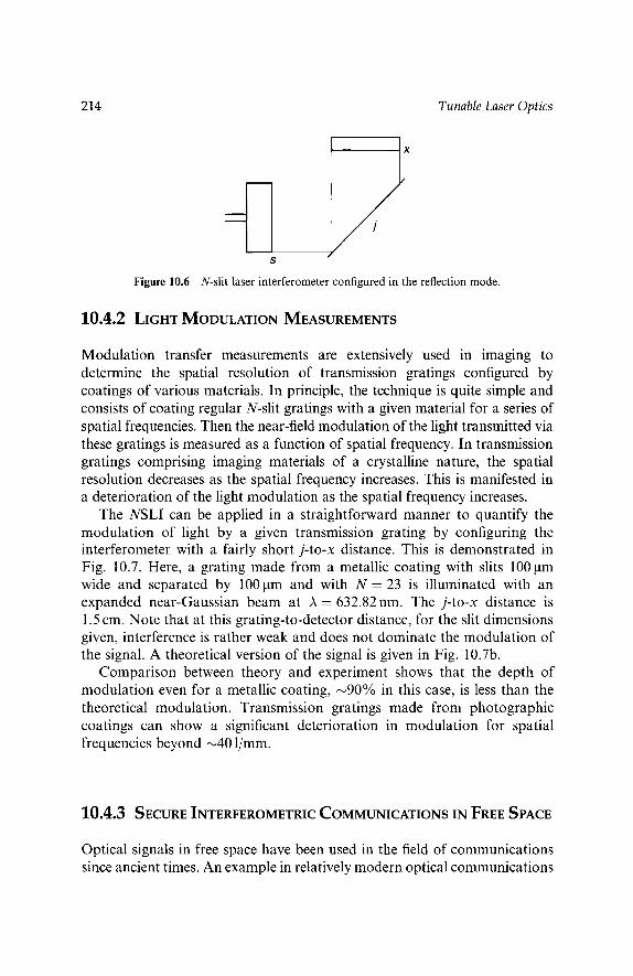
214 Tunable Laser Optics
$
I
Figure 10.6 N-slit laser interferometer configured in the reflection mode.
10.4.2 LIGHT MODULATION MEASUREMENTS
Modulation transfer measurements are extensively used in imaging to determine the spatial resolution of transmission gratings configured by coatings of various materials. In principle, the technique is quite simple and consists of coating regular N-slit gratings with a given material for a series of spatial frequencies. Then the near-field modulation of the light transmitted via these gratings is measured as a function of spatial frequency. In transmission gratings comprising imaging materials of a crystalline nature, the spatial resolution decreases as the spatial frequency increases. This is manifested in a deterioration of the light modulation as the spatial frequency increases.
The NSLI can be applied in a straightforward manner to quantify the modulation of light by a given transmission grating by configuring the interferometer with a fairly short j-to-x distance. This is demonstrated in Fig. 10.7. Here, a grating made from a metallic coating with slits 100 ~tm wide and separated by 100~tm and with N = 23 is illuminated with an expanded near-Gaussian beam at A = 632.82nm. The j-to-x distance is 1.5 cm. Note that at this grating-to-detector distance, for the slit dimensions given, interference is rather weak and does not dominate the modulation of the signal. A theoretical version of the signal is given in Fig. 10.7b.
Comparison between theory and experiment shows that the depth of modulation even for a metallic coating, ,--,90% in this case, is less than the theoretical modulation. Transmission gratings made from photographic coatings can show a significant deterioration in modulation for spatial frequencies beyond ,-,401/mm.
10.4.3 SECURE INTERFEROMETRIC COMMUNICATIONS IN FREE SPACE
Optical signals in free space have been used in the field of communications since ancient times. An example in relatively modern optical communications
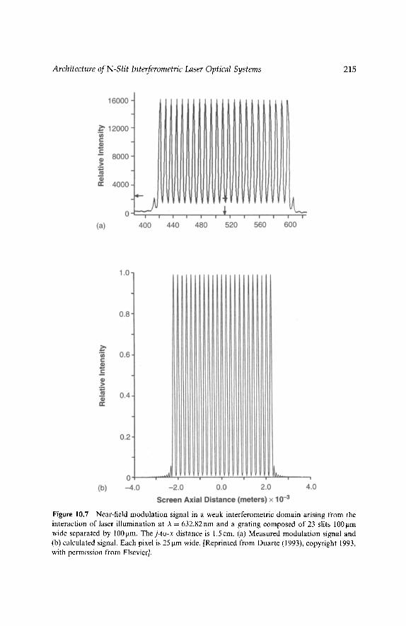
Architecture of N-Slit Interferometric Laser Optical Systems 215
Figure 10.7 Near-field modulation signal in a weak interferometric domain arising from the interaction of laser illumination at A = 632.82 nm and a grating composed of 23 slits 100 ~tm wide separated by 100 pm. The j-to-x distance is 1.Scm. (a) Measured modulation signal and (b) calculated signal. Each pixel is 25 l, tm wide. [Reprinted from Duarte (1993), copyright 1993, with permission from Elsevier].

216 Tunable Laser Optics
is the use of Morse code. More recent interest in this field has produced a variety of laser-based optical architectures and approaches (Yu and Gre- gory, 1996; Boffi etal., 2000; Willebrand and Ghuman, 2001). Prevalent among the approaches offering secure communications is quantum crypto- graphy (Jacobs and Franson, 1996). Here, an alternative approach to secure optical communications in free space, based on interferometric communica- tions, is introduced and described.
For a given set of geometrical parameters and wavelength, the NSLI yields a unique interferogram that can be matched to its theoretical counter- part. This feature can be utilized in the field of optical communications to perform secure communications in free space. The optical architecture of the NSLI used for this application is as described previously, with the one modification that the distance from the N-slit array (j) to the digital detector (x) can be very large, and allowances are made for a beam splitter, repre- senting a possible intruder, to be inserted in the optical path between j and x. This modified, long-path NSLI is depicted in Fig. 10.8.
The principle of operation is rather simple: Any optical distortion intro- duced in the optical path between j and x alters the predetermined interfero- gram recorded at x. Thus the receiver at x immediately detects the presence of an intruder or eavesdropper in the optical path of communications. Thus, interferometric communications provide a simple alternative to secure com- munications in free space. The method is particularly suited for providing secure communications in outer space.
As described by Duarte (2002), secure interferometric communications using the NSLI relies on an interferometric alphabet in which an alphabetic character, such as an a, is related to a specific interferogram. Four possible characters corresponding to a, b, c, and z are shown in Fig. 10.9. Here, the a is represented by two slits, the letter b by three slits, the letter c by four slits, and so on. The slits are 50 lam wide and are separated by 50 ~m at A -- 632.82 nm. Certainly, there is a limitless choice of alphabetic characters.
s 1
x
Figure 10.8 NSLI configured with a very longj-to-x path for interferometric communications.

Architecture of N-Slit Interferometric Laser Optical Systems
2.5
217
2.0
r t - o 1.5
.i,,a t--
( l )
N 1.o
0.5
o.o ~ . . . . . - 2 . 5 - 2 . 0 - 1 . 5 - 1 . 0 - 0 . 5 0.0 0.5 1.0 1.5 2.0 2.5
Distance (meters) x 10 -3
3.5
(a)
3.0-
~, 2.5"
2.0 o.) .=> ~.5i rr 1.0
0.5
0.0 ~ - - | , !
-2.5- :2.0-1 ' .5 '1'.0-0'.5 0J0 0.5 1.0 Distance (meters) x 10 .3
# l
1.5 2.0 2.5
(b)
4 . 0
3.5
._>, 3.0 t/) = 2.5 o
2.0 o 2 _~ ~.5 rr 1.0
0.5
0.0, , 7 " - ~ c i i i i
- 2 . 5 - 2 . 0 - 1 . 5 - 1 . 0 - 0 . 5 0.0 0.5 1.0 1.5 2.0 2.5 Distance (meters) x 10 -3
(c)
Figure 10.9 Interferometric alphabet. (a) a, (b) b, (c) c, and (d) z. [Reprinted from Duarte (2002), copyright 2002, with permission from Elsevier].

218 Tunable Laser Optics
4.5
4.0
' 3.5
-~ 3.0 r O "-" 2.5 r
( I ) > 2.0 . m
-~ 1.5 r r
1.0
0.5
0 . 0 -3.o -i.o olo 1.'o z'o 3.0
Distance (meters) x 10 -3
Figure 10.9 (Continued).
(d)
Transmission integrity is demonstrated in Fig. 10.10 for the case of the interferometric character a. To this effect an optically smooth surface with an average thickness of ~ 150 ~tm is introduced at an angle in the optical path to cause a reflection of the character a. It should be noted that insertion of the beam splitter normal to the optical axis produces no measurable spatial optical distortions except a decrease in the intensity of ~8%.
The angle of incidence of the interferometric character on the beam splitter was selected to be close to the Brewster angle of incidence to reduce transmission losses while still being able to reflect a measurable fraction of the signal. In the sequence of measurements, Fig. 10.10a shows the undis- torted character a. The severe distortions depicted in Figs. 10.10b to 10.10d show the effect of introducing the thin beam splitter in the optical path. Fig. 10.10e depicts the intercepted interferometric character a. Although the severe distortions are no longer present, close scrutiny of the interferogram reveals a decrease by ,-.,3.7% in the intensity of the signal relative to the original character shown in Fig. 10.10a. The intercepted signal is also displaced by approximately 50 ~tm in the frame of reference of the detector due to the refraction induced at the beam splitter. In addition, there is a slight obliqueness in the intensity distribution as determined from the secondary maxima. Hence, by comparison with the original interferometric character or a theoretically generated character, it can be concluded that the integrity of the intercepted character a has been distinctly compromised.
Although the measurements just considered were performed over short propagation path lengths in the laboratory (0.1 m and 1 m), Duarte (2002) also discusses propagation over larger distances. Using interferometric

8000- _~ c 6000
.~ 4000
E 2000
0
9000-
|
460 480 500 520 540 560 Numberof Pixels
"~ 7000 C
.~ 5000
3000 E
1000
2600-
.~ 2200 ~ oO e -
_~ 18oo~ _= .~ ~4oo~
looo~ ~" 600:
2O0
460 480 560 520 540 560 Number of Pixels
9000-
' | . . . . . | | w i !
460 480 500 520 540 560 Number of Pixels
(a)
(b)
(c)
219
"~ 7000 E
~ -
�9 5000 .5
3000
1000-
460 480 500 520 540 560 Number of Pixels
Architecture of N-Slit Interferometric Laser Optical Systems
(d)
Figure 10.10 Interception sequence of the interferometric character a (see text for details). [Reprinted from Duarte (2002), copyright 2002, with permission from Elsevier].

220
>, 80001 = �9 6000 t _c
e~ 000t 2 4 rr
0~'- , -~-~, ; , . 460 480 500 520 540 560
Number of Pixels
Figure 10.10 (Continued).
Tunable Laser Optics
(e)
calculations, via Eq. (10.2) or (10.3), it can be shown that communication in free space can proceed over long path lengths using visible wavelengths and a detector comprising of a few tiled photodiode arrays. One specific example involves the generation of the interferometric character a using two 1 mm slits separated by 1 mm. For A = 632.82 nm, this arrangement produces an interferometric distribution bound within 10cm for a propagation path length of 100 m. The interferometric character z is produced by an array of 26 slits of 1 mm separated by 1 mm. For A = 632.82 nm, this arrangement produces an interferometric distribution bound within 14 cm for a propaga- tion path length of 100 m. This can be accomplished using two off-the-shelf linear photodiode arrays (each 72 mm long) tiled together. If the dimensions of the slits are increased to 3 mm at A = 441.56 nm, interferometric charac- ters could be propagated over distances of 1000m using four such tiled photodiode arrays (Duarte, 2002).
The examples considered here assume a propagation path characterized by a single homogeneous propagation medium, such as vacuum, between j and x. One modification would be the introduction of a distortionless beam expander, such as an optimized multiple-prism beam expander. In Chapter 4 it was shown that these expanders can easily provide beam magnification factors of M ~ 100. Deployment of such a multiple-prism beam expander next to the slit array would reduce the beam divergence significantly, thus reducing the requirements on the dimensions of the digital detectors.
Free-space communications of interferometric characters in terrestrial environments would need to account for the inherent atmospheric turbu- lence present in such surroundings. This would certainly detract from the simplicity of the method. This could still be accomplished by noting that atmospheric distortions are stochastic in nature as compared to systematic distortions introduced by optical interception.

Architecture of N-Slit Interferometric Laser Optical Systems 221
From a technological viewpoint, it is important to emphasize the use of TEM00 lasers with narrow-linewidth emission, since that characteristic is essen- tial in providing well-defined interferometric characters close to their theoretical counterparts. The characters could be changed in real time either by using a tunable laser (Duarte, 1999) or by incorporating precision variable-slit arrays. The use of narrow-bandpass filters could allow transmission during daylight.
Quantum cryptography provides secure optical communications guaran- teed by the uncertainty principle and has been shown to be applicable over distances of tens of kilometers (Jacobs and Franson, 1996). Interferometric communications using the NSLI provides security using the principles of diffraction, refraction, and reflection. As discussed in Chapter 2, all of these principles have their origin in the principle of interference. As outlined in Chapter 3, the uncertainty principle itself can be formulated from interfero- metric arguments. Advantages of free-space communications using inter- ferometric characters include a very simple optical architecture and the use of relatively high-power narrow-linewidth lasers, although, in principle, the method also applies to single-photon emission.
10.4.4 WAVELENGTH METER AND BROADBAND INTERFEROGRAMS
Generalized N-slit interference equations, such as Eqs. (10.2) and (10.3), are inherently wavelength dependent, since the interference term is a function of wavelength, as explained in Chapter 2. Thus, it is straightforward to predict that, for a given set of geometrical parameters, the measured interferogram depends uniquely on the wavelength of the laser. This feature can be applied to use of the NSLI as a wavelength meter, as will be explained in Chapter 11.
Although emphasis up to now has been placed on the desirability of using narrow-linewidth lasers in conjunction with the NSLI, the scope of the measurements can also be extended to include broadband emission. For broadband emission sources the measured interferogram represents a cumu- lative interferogram of a series of individual wavelengths of the form depicted in Fig. 10.11. This concept is central to this measurement approach, and it is based on Dirac's dictum on interference (Dirac, 1978). That is, interference occurs between undistinguishable photons only. In other words, blue photons do not interfere with green or red photons. Hence, an inter- ferogram with broad features, as illustrated in Fig. 10.11, is a cumulative signal composed of a series of individual interferograms arising from a series of different wavelengths. Once the central wavelength of emission of the broadband interferometer is determined using a standard spectrometer or suitable wavelength meter, a theoretical cumulative interferometer can be constructed to match the measured signal and determine its bandwidth.

222 Tunable Laser Optics
6000 ~-
5000 - >.,
t - 4000 0 ,r
.>__ 3000 ..b-,
I I 2000
1000
I I I I
4 6 0 4 8 0 500 520 540 560
Number of Pixels
Figure 10.11 Interferogram from broadband light source.
In principle, for broadband ultrashort pulsed lasers, once the bandwidth of the emission is determined, an approximate estimate of the temporal pulse duration is possible using the time-frequency uncertainty relation AuAt ~ 1. This simple concept is applicable only to ultrashort-pulse lasers emitting pulses and spectral distributions obeying the time-frequency uncertainty limit.
10.5 SENSITOMETRY
Traditional sensitometry and sensitometers are described by Altman (1977). In essence, a sensitometer is an instrument that illuminates an unexposed imaging material to produce a series of exposures at various light intensity levels. A laser sensitometer uses stable lasers yielding TEM00 beams and various optical techniques to produce a scale of exposures that can then be optically characterized to determine the sensitivity of the imaging material. In this section the optical architecture of a multiple-laser sensitometer is described.
Laser sensitometers work on the principle of exposing a line by displacing a focused near-Gaussian beam with a beam waist in the range 50 ~tm _< w _< 100 ~tm. This line is exposed on the imaging material, which is deployed at a plane perpendicular to the optical axis and to the plane of propagation. The imaging medium is displaced, orthogonal to the optical axis, at a velocity allowing for an overlap (usually 50%) of the near~ Gaussian beam. The movement of the laser beam provides the temporal component of the exposure. Once an exposure of certain dimensions is produced, usually 10 mm in width, the intensity of the laser beam is adjusted, using electro-optical means, and a new series of line exposures is produced.

Architecture of N-Slit Interferometric Laser Optical Systems 223
Eventually a scale of rectangular exposures at different laser intensity levels is rendered. Three optical channels, corresponding to blue, green, and red lasers, converging to a single exposure plane are often employed.
An alternative laser sensitometer is depicted in Fig. 10.12. This is a single- channel multiple-laser multiple-prism sensitometer using polarization to vary the intensity of the laser exposure. In this description the laser sensi- tometer will be referred to as a polarizer multiple-prism multiple-laser (PMPML) sensitometer.
The PMPML sensitometer (see Fig. 10.12) uses a single optical channel with a principal laser as the first element defining the optical axis and second- ary lasers adding their radiation via beam splitters. All lasers are polarized parallel to the plane of incidence. A variable broadband neutral-density filter is inserted as a coarse intensity control prior to the polarizer. The polarizer is a Glan-Thompson prism pair, with an extinction coefficient of 1 x 10 -6 or better, mounted on a high-precision annular rotational stage capable of an angular resolution of 0.001 arc sec. As described in Chapter 5, rotation of this polarizer causes the transmission of the lasers to decrease from nearly full transmission to close to total extinction. For the lasers polarized parallel to the plane of polarization, optimum transmission is accomplished with the Glan-Thompson polarizer deployed as depicted in Fig. 10.12.
Following the polarizer, the beams enter a telescope-lens system and a multiple-prism beam expander, as shown in Fig. 10.1. The elongated near- Gaussian beams are then propagated through a wide aperture so as to produce a diffractive profile, as depicted in Fig. 10.13. Note that the dif- fractive profile is wider than the width of the exposures needed, so the intensity variation caused by the "ears" of the profile do not affect the wanted area. The fine variations toward the center of the distribution have a negligible effect.
I I /'1 Laser 1 F
Telescope
Laser 2 Laser 3
Muliple-prism Wide Imaging beam expander slits plane
Figure 10.12 Polarizer multiple-prism laser sensitometer. The telescope expands the beam in two dimensions whilst the multiple-prism beam expander magnifies in only one dimension parallel to the plane of propagation.

224 Tunable Laser Optics
Figure 10.13 Diffraction profile of the illumination line at A = 532 nm.
Using the method just described, a line exposure is instantaneously pro- vided, thus eliminating the need to displace the laser beams and the asso- ciated electromechanical means necessary to accomplish this task. Since the line exposure is horizontal, the imaging material is displaced in a plane orthogonal to the plane of incidence of the instrument. In P M P M L sensito- meters the temporal exposures are provided by using the lasers in a pulsed mode. Thus, depending on the lasers, it is possible to vary the exposure time from less than 1 ns to 1000ns. It should also be mentioned that careful selection of the beam profiles of the lasers and their respective distances to the main optical axis enables spatial overlapping of the laser beams to within 1 ~tm at the focal plane with a minimal use of extra beam-shaping optics. As indicated by Duarte (2001), lasers suitable for illumination include mode- locked diode-pumped frequency-doubled Nd:YAG lasers and pulsed semi- conductor lasers.
PROBLEMS
1. For the telescope, lens, multiple-prism, distance architecture depicted in Fig. 10.1, derive its propagation ray transfer matrix given in Eq. (10.9).
2. Show that in the absence of a convex lens, Eq. (10.9) reduces to Eq. (10.16). 3. Show that in the absence of a convex lens, Eq. (10.15) reduces to
Eq. (10.17).
Architecture of N-Slit Interferometric Laser Optical Systems 225
4. Design a double-prism beam expander yielding zero dispersion at the wavelength of design and M = 5 for an optical system as depicted in Fig. 10.1. Using a Galilean telescope with Mt---20 and a convex lens with
f - 30 cm, calculate the width and the height of the resulting extremely elongated near-Gaussian beam at the focal plane. Assume a TEM00 He-Ne laser at A = 632.82 nm and w0 = 250 ~tm. For the material of the multiple-prism beam expander use fused silica.
5. For a beam splitter made of fused silica and a thickness of 1 mm, deter- mine the lateral displacement from its original path of a TEM00 He-Ne laser beam at A = 632.8 nm immediately following the beam splitter if the angle of incidence is 57 ~ .
REFERENCES
Altman, J. H. (1977). Sensitometry of black-and-white materials. In The Theory of the Photo- graphic Process (James, T. H., ed.). Eastman Kodak Company, Rochester, NY, pp. 481-516.
Boffi, P., Piccinin, D., Mottarella, D., and Martinelli, M. (2000). All-optical free-space process- ing for optical communications signals. Opt. Commun. 181, 79-88.
Dainty, J. C., and Shaw, R. (1974). Image Science. Academic Press, New York. Deutsch, D. (1992). Quantum computation. Phys. Worm 5(6), 57-61. Dirac, P. A. M. (1978). The Principles of Quantum Mechanics, 4th ed. Oxford University Press,
London. Duarte, F. J. (1985). Note on achromatic multiple-prism beam expanders. Opt. Commun. 53,
259-262. Duarte, F. J. (1987). Beam shaping with telescopes and multiple-prism beam expanders. J. Opt.
Soc. Am. A 4, p. 30. Duarte, F. J. (1991). Dispersive dye lasers. In High-Power Dye Lasers (Duarte, F. J., ed.).
Springer-Verlag, Berlin, pp. 7-43. Duarte, F. J. (1993a). On a generalized interference equation and interferometric measurements.
Opt. Commun. 103, 8-14. Duarte, F. J. (1993b). Electro-optical interferometric microdensitometer system. U.S. Patent
No. 5,255,069. Duarte, F. J. (1995). Interferometric imaging. In Tunable Laser Applications (Duarte, F. J., ed.)
Marcel Dekker, New York, pp. 153-178. Duarte, F. J. (1996). Generalized interference equation and optical processing. In Proceedings of
the International Conference on Lasers '95 (Corcoran, V. J., and Goldman, T. A., eds.). STS Press, McLean, VA, pp. 615-617.
Duarte, F. J. (1999). Multiple-prism grating solid-state dye laser oscillator: optimized architec- ture. Appl. Opt. 38, 6347-6349.
Duarte, F. J. (2001). Laser sensitometer using multiple-prism beam expansion and a polarizer. U.S. Patent no. 6,236,461.
Duarte, F. J. (2002). Secure interferometric communications in free space. Opt. Commun. 205, 313-319.
Duarte, F. J., and Paine, D. J. (1989). Quantum mechanical description of N-slit interference phenomena. In Proceedings of the International Conference on Lasers '89 (Harris, D. G., and Shay, T. M., eds.). STS Press, McLean, VA, pp. 42-27.

226 Tunable Laser Optics
Duarte, F. J., and Piper, J. A. (1982). Dispersion theory of multiple-prism beam expanders for pulsed dye lasers. Opt. Commun. 43, 303-307.
Jacobs, B. C., and Franson, J. D. (1996). Quantum cryptography in free space. Opt. Lett. 21, 1854-1856.
Turunen, J. (1986). Astigmatism in laser beam optical systems. Appl. Opt. 25, 2908-2911. Willebrand, H. A., and Ghuman, B. S. (2001). Fiber optics without fiber. IEEE Spectrum 38(8),
40-45. Yu, S. T. S., and Gregory, D. A. (1996). Optical pattern recognition: architectures and techni-
ques. Proc. IEEE 84, 733-752.

Chapter 11
Spectrometry and Interferometry
11.1 I N T R O D U C T I O N
Laser optics employs several diagnostic tools. Characterization of pulsed laser emission requires measurements of the following parameters: energy and/or power, temporal profile of laser pulses, spatial characteristics of the laser beam, wavelength, and linewidth. Characterization of CW laser emis- sion requires measurements of power, spatial characteristics of the laser beam, wavelength, and linewidth.
Measurements of laser energy and power employ optoelectric and/or thermoelectric detectors. Determination of temporal profiles requires opto- electric detection and display electronics, for pulses down to the nanosecond regime, and autocorrelators (Diels, 1990; Diels and Rudolph, 1996) or other specialized instrumentation, such as frequency-resolved optical gating (Trebino et al., 1997), for pulses in the femtosecond domain. In this chapter, attention is focused on instrumentation useful in the measurement of laser wavelength and linewidth.
11.2 SPECTROMETRY
Spectrometry, in principle, depends on the interaction of a light beam with a dispersive element or dispersive elements and on spatial discrimination following postdispersive propagation. Hence, the higher the dispersive
227

228 Tunable Laser Optics
power and the longer the optical path of the postdispersive propagation, the higher the wavelength resolution. As described in earlier chapters, dispersion can be provided by either prisms, gratings, or prism-grating combinations.
For a detailed treatment on the subject of spectrometry the reader should refer to Meaburn (1976).
11.2.1 PRISM SPECTROMETERS
Prism spectrometry has its origin in the experiments reported by Newton (1704) in his book Opticks. Prism spectrometers usually deploy equilateral or isosceles prisms in series to augment the dispersion of the instrument. As described in Chapter 4, for an array of r identical isosceles or equilateral prisms deployed symmetrically in an additive configuration so that q~l, 1 = ~)1,2 . . . . . q~l,m and q~l,m -- q~2, m, the cumulative dispersion is given by (Duarte, 1990)
~7A~)2, r = r~Taq~2,1 (11.1)
V~q52,~ - ((sin ~2,1/ cos 4~2,1)+ (COS~2,1/COS4~2,1) tan~l,1)V~n (11.2)
where all angular parameters are as described in Chapter 4. These equations indicate that dispersion can be augmented by a combination of two factors: increasing the number of prisms and using prisms with a high material dispersion. For some materials, V:~n is given in Table 4.1.
Prism spectrometers assume various configurations. Two of these are considered here. The first configuration, depicted in Fig. 11.1, uses two prisms in series, with a considerable distance between the two prisms to increase the overall angular spread of the emerging beam. Long postdisper- sive optical paths of up to 3 meters, in conjunction with narrow apertures,
Figure 11.1 Long-optical-path double-prism spectrometer.

Spectrometry and Interferometry 229
provide wavelength resolutions in the nanometer range. The second archi- tecture, described by Meaburn (1976), includes a sequence of several prisms in series, as depicted in Fig. 11.2. In this configuration, dispersion is simply augmented by a larger factor r in Eq. (11.1). The same observations about the postdispersive optical path and spatial discrimination are relevant.
1 1 . 2 . 2 DIFFRACTION G R A T I N G SPECTROMETERS
As described in Chapter 2, the diffraction grating equation is given by
d(sin O + sin ~) = mA (11.3)
and the angular dispersion is obtained by differentiating this equation so that
O0/OA = m/(acos O) (11.4)
or alternatively
00/0A = (sin O + sin ~)/(A cos O) (11.5)
For a grating deployed in Littow configuration, O = �9 and the grating equation becomes
2d sin O = mA (11.6)
and the dispersion can be expressed as
00/0A = 2 tan O/A (11.7)
As with prismatic spectrometers, the three factors that increase wave- length resolution in a diffraction grating spectrometer are dispersion, optical path length, and the dimensions of the aperture at the detection plane. From Eq. (11.4) it is clear that one avenue to increase dispersion is to use gratings deployed at a higher order or to employ gratings with a high groove density.
Figure 11.2 Dispersive assembly of multiple-prism spectrometer. The angle of incidence (~l,m and the angle of emergence 4~2,m are identical for all prisms. In addition to the cumulative dispersion, resolution is determined by the path length toward the exit slit and the dimensions of the slit.
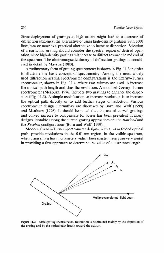
230 Tunable Laser Optics
Since deployment of gratings at high orders might lead to a decrease of diffraction efficiency, the alternative of using high-density gratings with 3000 lines/ram or more is a practical alternative to increase dispersion. Selection of a particular grating should consider the spectral region of desired oper- ation, since high-density gratings might cease to diffract toward the red end of the spectrum. The electromagnetic theory of diffraction gratings is consid- ered in detail by Maystre (1980).
A rudimentary form of grating spectrometer is shown in Fig. 11.3 in order to illustrate the basic concept of spectrometry. Among the most widely used diffraction grating spectrometer configurations is the Czerny-Turner spectrometer, shown in Fig. 11.4, where two mirrors are used to increase the optical path length and thus the resolution. A modified Czerny-Turner spectrometer (Meaburn, 1976) includes two gratings to enhance the disper- sion (Fig. 11.5). A simple modification to increase resolution is to increase the optical path directly or to add further stages of reflection. Various spectrometer design alternatives are discussed by Born and Wolf (1999) and Meaburn (1976). It should be noted that the use of curved gratings and curved mirrors to compensate for losses has been prevalent in many designs. Notable among the curved-grating approaches are the Rowland and the Paschen configurations (Born and Wolf, 1999).
Modern Czerny-Turner spectrometer designs, with a ~4 m folded optical path, provide resolutions in the 0.01-nm region, in the visible spectrum, when using slits a few micrometers wide. These spectrometers are very useful in providing a first approach to determine the value of a laser wavelength.
'~m
ha "~2
,kl
Grating ~
Figure 11.3 Basic grating spectrometer. Resolution is determined mainly by the dispersion of the grating and by the optical path length toward the exit slit.

Spectrometry and Interferometry 231
sl I
I s2
1
Figure 11.4 Czerny-Turner spectrometer. Mirrors M1 and M2 provide the necessary curvature to focus the diffracted beam at the exit slit. Widely used spectrometers of this type often have an optical path length between the entrance slit and the back mirror in the range 25-100cm.
I M1
G
S21 M2 Figure 11.5 Double-grating Czerny-Turner spectrometer. Mirrors M1 and M2 provide the necessary curvature to focus the diffracted beam at the exit slit.
11 .2 .3 DISPERSIVE WAVELENGTH METERS
Dispersive wavelength meters are in essence dispersive spectrometers with the conventional slit-detector arrangement replaced by a linear photodiode array or CCD detector. Their main function is to determine the wavelength from the emission of tunable lasers. The resolution is determined by the available dispersion, the propagation distance between the dispersive ele- ment and the detector array, and the dimensions of the individual pixels at the digital array. Depending on the type of detector, individual pixels vary in size from a few micrometers to ~25 lam in width. The typical width of these digital arrays varies from ~25 mm to ~ 5 0 m m . This type of wavelength meter is used in conjunction with well-known, and preferably stabilized, laser sources for calibration. Morris and McIlrath (1979) used a 40-cm spectrometer incorporating an echelle grating deployed at a high order in conjunction with a photodiode array integrated by 1024 elements (each ~25 mm wide) to determine wavelengths within 0.01 nm in the visible.

232 Tunable Laser Optics
A wavelength meter based on a high-dispersion prism-grating configur- ation is illustrated in Fig. 11.6. As discussed in Chapter 4, the dispersion of a diffraction grating can be significantly augmented when deployed with prism assemblies according to (Duarte and Piper, 1982)
, , - ( , ' ) ~7A~l, m __ ~ t ~ l ,rn ~ A ?,lrn _+_ ( ktl ,m k t2 ,m ) 1 ~ 2 ,m ~ A Flrn -4- ~7Aq~l,(rn+l) (l 1.8)
where
VA~tl,(m+l) = (VAOG q-- VA~2, r) (1 1.9)
Here, VxOG is the grating dispersion and V~r is the single-pass prism dispersion. For a single prism, as depicted in Fig. 11.6, r = 1 and
VAr = tanr (11.10)
Using a 600-1ines/mm echelle grating deployed in the third order and a BK-7 optical glass prism (n = 1.512 at A = 568.8 nm) with an apex angle of 41.5 ~ the sensitivity of the system becomes 0.3 ~ nm -1 (Duarte, 1983). For a 1000-mm distance from the prism to the detector, this dispersive combination can measure wavelengths with a 0.01-nm resolution. Absolute wavelength cali- bration was provided by the spectrum of molecular iodine and the I2 spectral atlas of Gerstenkorn and Luc (1978). Once calibrated, this simple prism- grating wavelength meter configuration offers static operation and can be
Grating
1
Photodiode ~j'
_., ~R,~M~ ~'R ~,
S
~'M
Figure 11.6 Prism-grating wavelength meter. (From Duarte, 1983.)
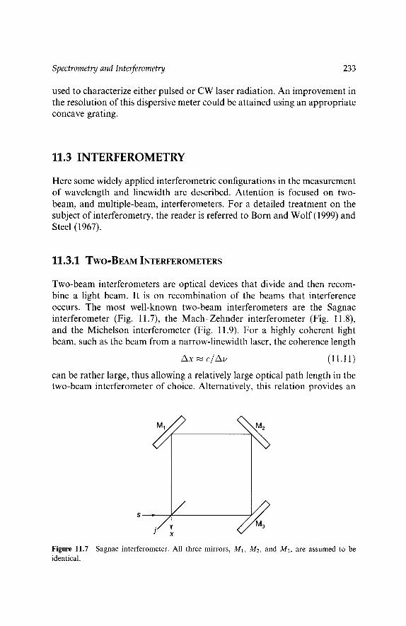
Spectrometry and Interferometry 233
used to characterize either pulsed or CW laser radiation. An improvement in the resolution of this dispersive meter could be attained using an appropriate concave grating.
11.3 INTERFEROMETRY
Here some widely applied interferometric configurations in the measurement of wavelength and linewidth are described. Attention is focused on two- beam, and multiple-beam, interferometers. For a detailed treatment on the subject of interferometry, the reader is referred to Born and Wolf (1999) and Steel (1967).
1 1 . 3 . 1 T w o - B E A M INTERFEROMETERS
Two-beam interferometers are optical devices that divide and then recom- bine a light beam. It is on recombination of the beams that interference occurs. The most well-known two-beam interferometers are the Sagnac interferometer (Fig. 11.7), the Mach-Zehnder interferometer (Fig. 11.8), and the Michelson interferometer (Fig. 11.9). For a highly coherent light beam, such as the beam from a narrow-linewidth laser, the coherence length
A x ~ c l A u (11.11)
can be rather large, thus allowing a relatively large optical path length in the two-beam interferometer of choice. Alternatively, this relation provides an
S /
J x
Figure 11.7 Sagnac interferometer. All three mirrors, M1, M2, and M2, are assumed to be identical.

234
k / ~X
Figure 11.8 Mach-Zehner interferometer.
Tunable Laser Optics
1 j Y
/
I I
Figure 11.9 Michelson interferometer.
avenue to accurately determine the linewidth of a laser by increasing the optical path length until interference ceases to be observed.
Interference in the Sagnac interferometer can be described using Dirac notation via the probability amplitude
N N
(xls) = Z Z (x[j')Q''[l')Q'[s) (11.12) j '= l j=l
where j represents the reflection surface of the beam splitter and the prob- ability amplitude (j'[/') represents the trip around the interferometer, which includes reflections at mirrors M1, M2, and M3. Assuming that
(j'[j) = 1 (11.13)

Spectrometry and Interferometry 235
Eq. (11.12) reduces to
which, for N - 2, becomes
N
(x[s) - ~ (x[/') (/'Is) (11.14) j = l
(sis) - (xl2)(2Is) + (Nil)(1 Is) (11.15)
Here, j - 1 represents the beam splitter in a reflection mode and j - 2 represents the beam splitter in a transmission mode.
Interference in the Mach-Zehnder interferometer can be described using
N N
(xls) - ~ ~ (xlk)(k[/) (/'Is) (11.16) k=l j = l
for N = 2. Again, if j represents the entrance beam splitter and k the exit beam splitter, we can write
(x[s) = (x]l)(1 [2)(21s ) + (xl l) (1] l) (1]s) + (x]2)(212)(2Is) + (x12) (211)(1 Is)
(11.17)
Here, j = k = 1 represents the beam splitters in a reflection mode and j = k = 2 represents the beam splitter in a transmission mode. Since (1[1) and (212) lead to x t rather than x, the probability amplitude for this geome- try reduces to
(x]s) = (x] l) (112) (2]s) + (x]2) (2] l) (1]s) (11.18)
For the Michelson interferometer the interference can be characterized using a probability amplitude of the form
N N
f = l j = l
where j = 1 represents the function of the beam splitter in the reflection mode and j = 2 represents the function of the beam splitter in the transmis- sion mode. In a second-pass approach, j ' = 1 represents the function of the beam splitter in a transmission mode and f = 2 represents the function of the beam splitter in a reflection mode. Since reflection on the first pass (j = 1) and reflection on the second pass ( f = 2) lead back to s, and likewise j = 2 followed by and f = 1, Eq. (11.12) reduces to
(x]s) - (x]2)(2]2)(2[s)+ (xl l) (l l l) (l ls) (11.19)

236 Tunable Laser Optics
Here, (111) represents a change at j from reflection to transmission and (212) represents a change from transmission to reflection. It is clear that multi- plication of Eqs. (11.15), (11.18), and (11.19)with their respective complex conjugates yields probability equations of an interferometric character.
11.3.2 MULTIPLE-BEAM INTERFEROMETERS
An N-slit interferometer, which can be considered a multiple-beam inter- ferometer, was introduced in Chapter 2 and is depicted in Fig. 11.10. In this configuration, an expanded beam of light illuminates simultaneously N slits. Following propagation the N subbeams interfere at a plane perpendicular to the plane of propagation. The probability amplitude is given by
N
<.l.> - Z <,l.> j=]
and the probability is
N N
I(xls)l= - (rj) t~(rm)e i(f~m-f~;) (11.20) j = l m=l
which can also be expressed as (Duarte, 1991, 1993)
I(xls)12 - j~=l ~(rj)2 + 2 ~ t p ( r j ) t~(rm) COS(Qm -- ~j) (11.21) j = l m=j+l
Expressions for two-dimensional and three-dimensional cases are given in Chapter 2. This approach is also applicable to the two-beam interferometer introduced by Hambury-Brown and Twist (1956) (shown in Fig. 11.11) and
s j x
/ Expanded
TEMoo laser beam
N-slit array
Figure 11.10 N-slit interferometer.
Diode array
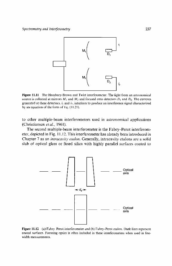
Spectrometry and Interferometry 237
I I
M1 D1
M2 I I~ D2
Figure 11.11 The Hambury-Brown and Twist interferometer. The light from an astronomical source is collected at mirrors M1 and M2 and focused onto detectors D~ and D2. The currents generated at these detectors, il and i2, interferes to produce an interference signal characterized by an equation of the form of Eq. (11.21).
to other multiple-beam interferometers used in astronomical applications (Christiansen et al., 1961).
The second multiple-beam interferometer is the Fabry-Perot interferom- eter, depicted in Fig. 11.12. This interferometer has already been introduced in Chapter 7 as an intracavity etalon. Generally, intracavity etalons are a solid slab of optical glass or fused silica with highly parallel surfaces coated to
r -I Optical axis
Optical axis
Figure 11.12 (a) Fabry-Perot interferometer and (b) Fabry-Perot etalon. Dark lines represent coated surfaces. Focusing optics is often included in these interferometers when used in line- width measurements.

238 Tunable Laser Optics
increase reflectivity (Fig. l l.12a). These are also known as Fabry-Perot etalons. Fabry-Perot interferometers, on the other hand, are constituted by two separate slabs of optical flats with their inner surfaces coated, as shown in Fig. l l.12b. The space between the two coated surfaces is filled with air or some other inert gas. The optical flats in a Fabry-Perot inter- ferometer are mounted on rigid metal bars with a low thermal expansion coefficient, such as invar. The plates can be moved, with micrometer preci- sion or better, to vary the free spectral range (FSR). These interferometers are widely used to characterize and quantify the laser linewidth.
The mechanics of multiple-beam interferometry can be described in some detail by considering the multiple reflection and refraction of a beam incident on two parallel surfaces separated by a region of refractive index n, as illustrated in Fig. 11.13. In this configuration, at each point of reflection and refraction a fraction of the beam, or a subbeam, is transmitted toward the boundary region. Following propagation these subbeams interfere. In this regard, the physics is similar to that of the N-slit interferometer, with the exception that each parallel beam has less intensity due to the increasing number of reflections. Here, for transmission, interference can be described
k j r' r'
(a)
de
(b) --~1 D I-~--
Figure 11.13 Multiple-beam interferometer. (a) Multiple internal reflection diagram and (b) detailed view depicting the angles of incidence and refraction.

Spectrometry and Interferometry 239
using a series of probability amplitudes representing the events depicted in Fig. 11.13:
N N N N
- E Z Z: m=l l=1 k=l j=l
(11.22)
where j is at the reflection surface of incidence, k is immediately next to the surface of reflection, l is at the second surface of reflection, and m is immediately next to the second surface of reflection, as illustrated in Fig. 11.13. The problem can be simplified considerably if the incident beam is considered a narrow beam incident at a single point j. Propagation of the single beam then proceeds to I and is represented by the incidence amplitude A;, which is a complex number, attenuated by the transmission factor t, so the first three probability amplitudes can be represented by an expression of the form
{l[k) {k[l') {its) - Ait (11.23)
and Eq. (11.22) reduces to
N
{xls} -- Ait ~ {x m} Imil} m=l
(11.24)
which, using the notation of Born and Wolf (1999), can be expressed as
-- Ait(tt_}_ ttrt2e i<5 + ttrt4e i2<5 -Jr-...-+-ttrt2(p-1)ei@-') ~5) At(p) (1 1.25)
Defining
o_7 = t{ (11.26)
-- r '2 (11.27)
and taking the limit as p --+ e~, Eq. (11.25) reduces to (Born and Wolf, 1999)
A t - o_~(1- ~ei6)-lAi (11.28)
and multiplication with its complex conjugate yields this expression for the intensity:
It c:~2(1 + ~ 2 2 ~ C O S ( 5 ) -1 - - - - I i (11.29)
which is known as the Airy formula or Airy function. Plotting the ratio of the two intensities as a function of
~5 = 27rm (11.30)

240 Tunable Laser Optics
shows that the contrast of the fringes increases as the reflectivity increases (Born and Wolf, 1999). From the geometry of Fig. 11.13, the path difference between the first reflected beam and the first beam that undergoes internal reflection followed by refraction is
A L = 2nde sec ~e - 2nde tan ~e sin ~e (11.31)
which reduces to
A L -- 2nde cos ~e (11.32)
Hence, using AL = mA and the definition given in Eq. (11.30), the phase can be expressed as
6 = 47rndeA -1 cos ~e (11.33)
where n is the refractive index of the medium and de is the distance between the reflection surfaces.
The device just described is an uncoated interferometer. If the two sur- faces of the plate are coated with metal films of equal reflectivity, the phase term takes the form of (Born and Wolf, 1999)
6 = 47rndeA -1 cos ~e + 2qD (11.34)
and the multiple-beam interferometer is classified as a Fabry-Perot etalon. An interferogram produced by the interaction of narrow-linewidth laser emission and a Fabry-Perot etalon followed by a convex lens of focal length f is shown in Fig. 11.14. Here, the bright fringes, or rings, correspond to the maximum value of m, which is
which can be expressed as
mo -- 2ndeA -1 + ~ / 2 (11.35)
mo = 2ndeA -1 + e (11.36)
where e is the fractional fringe order. Using these equations the diameter of the rings is given by (Born and Wolf, 1999)
D 2 - ( 4 n A f 2 / n Z d e ) ( p - 1 + e) (11.37)
where p = 1,2,3,.. . and no is the refractive index of the surrounding medium.
The free spectral range (FSR) of a Fabry-Perot interferometer, or Fabry- Perot etalon, corresponds to the difference in wavelength of two adjacent orders. From Eq. (11.33) for a small angle of incidence,
m ~ 2ndeA -1 (11.38)
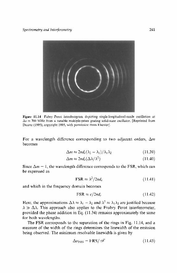
Spectrometry and Interferometry 241
Figure 11.14 Fabry-Perot interferogram depicting single-longitudinal-mode oscillation at Au ~ 700 MHz from a tunable multiple-prism grating solid-state oscillator. [Reprinted from Duarte (1995), copyright 1995, with permission from Elsevier].
For a wavelength difference corresponding to two adjacent orders, Am becomes
A m ,~ 2nde(A2 - A1)/A1A2 (11.39)
A m '~ 2nde(AA/A 2) (11.40)
Since Am = 1, the wavelength difference corresponds to the FSR, which can be expressed as
FSR ~ A 2/2nde (11.41)
and which in the frequency domain becomes
FSR ~ c/2nde (11.42)
Here, the approximations AA ~ A1 - ~2 and )k 2 ~,~ ~1 ~2 are justified because A >> AA. This approach also applies to the Frabry-Perot interferometer, provided the phase addition in Eq. (11.34) remains approximately the same for both wavelengths.
The FSR corresponds to the separation of the rings in Fig. 11.14, and a measure of the width of the rings determines the linewidth of the emission being observed. The minimum resolvable linewidth is given by
A U F R S - - FRS/~,~ (11.43)

242 Tunable Laser Optics
where ~ - is the effective finesse. Thus, a Fabry-Perot etalon with FSR = 7.49GHz and ~ = 50 provides discrimination down to only ~150 MHz. The finesse is a function of the flatness of the surfaces (often in the range A/100-A/50), the dimensions of the aperture, and the reflectivity of the surfaces. The effective finesse is given by (Meaburn, 1976)
Q ~ - - 2 Q_~-R 2 + ~ F 2 + Q.~-A 2 (11.44)
where ~ n , ~ - F and d~-A are the reflective, flatness, and aperture finesses, respectively. The reflective finesse is given by (Born and Wolf, 1999)
Q-~R -- 7rV/-~/(1 -- ~ ) (11.45)
11.3.3 INTERFEROMETRIC WAVELENGTH METrRS
Interferometry signals and profiles are a function of the wavelength of the radiation that produces them. Thus, interferometers are well suited to be applied as wavelength meters, especially when a digital detector array is used to record the resulting interferogram. As such, a variety of interferometric configurations have been used in the measurement of tunable laser wave- lengths. For a review on this subject, the reader should refer to Demtr6der (1995).
The wavelength sensitivity of multiple-beam interferometry has its origin in the phase information of the equations describing the behavior of the interferometric signal. In the case of the N-slit interferometer, the interfero- metric profile is characterized by Eq. (11.21), which includes a phase- difference term that, as explained in Chapter 2, can be expressed as
COs((O m -- Oj) -'1- (~)m -- ~ j ) ) - - COS(l/m -- l m - l l k l ~ ILm - t m - 1 ] k 2 ) (11.46)
where
kl = 27rnl/Av (11.47)
k2 = 27rn2/Av (11.48)
Here, A1 = Av/nl and A2 = Av/n2, where Av is the vacuum wavelength and nl and n2 are the corresponding indexes of refraction (Wallenstein and H~insch, 1974; Born and Wolf, 1999). Hence, it is easy to see that different wavelengths will produce different interferograms. To illustrate this point, in Fig. 11.15 four calculated interferograms, using Eq. (11.21), for the N-slit interferometer, with N = 50, are shown. For a given set of geometrical parameters, measured interferograms can be matched, in an iterative pro- cess, with theoretical interference patterns to determine the wavelength of

Spectrometry and Interferometry 243
Figure 11.15 Interferograms at (a) A1-'-580nm, (b))k 2 - -585nm, (c) A3 = 590nm, and (d) A4 = 591 nm. These calculations are for slits 100 gm wide, separated by 100 gin, and N = 50. The j to x distance is 100 cm.

244 Tunable Laser Optics
Figure 11.15 (Continued).
the radiation. Again, resolution depends on the optical path length between the slit array and the digital detector and on the size of the pixels and the linearity of the detector.
For a multiple-beam interferometer, the transmission intensity is given by Eq. (11.29), where, in reference to Fig. 11.13, the phase term 6 can be

Spectrometry and Interferometry 245
/
I
/ / /
IFSR n I ~ fn
]FSR2 ~ f 2
. . D n . . D 2
FSR~
, , D 1
Figure 11.16 Multiple-etalon wavelength meter.
expressed by Eq. (11.34), which depends on the reciprocal of the wavelength. Thus, recording of the transmission interferometric signal by a photodiode array or CCD array yields information on the wavelength of the radiation.
Wavelength meters based on Frabry-Perot interferometers generally involve configurations with multiple etalons in parallel (Byer etal., 1977; Fischer etal., 1981; Konishi etal., 1981). In the multiple-etalon con- figuration, depicted in Fig. 11.16, each etalon has a different FSR, which is compatible with the FSR and the finesse of the next etalon. For instance, Fischer et al. (1981) used three etalons with FSRs of 1000 GHz, 67 GHz, and 3.3GHz. Briefly, the methodology of this measurement consists in the application of Eqs. (11.36) and (11.37) to determine A with reduced uncer- tainty at each etalon. Using this approach, Fischer etal. (1981) report measurements of laser frequencies with an accuracy of 60 MHz.
A simple interferometric configuration that is used widely in the measure- ment of laser wavelengths is that of the Fizeau, or optical wedge, two-beam interferometer, first introduced by Snyder (1977). In this configuration the incident laser beam propagates on an axis that is at an angle to the optical axis of the digital detector, as depicted in Fig. 11.17. Also, the incident beam illuminates a wide area of the interferometer using some beam expansion method in conjunction with a spatial filter. The interference of the two beams is recorded by a digital detector with a 25-gm resolution or better. The method employs two predetermined parameters: the angle of the wedge and the wedge separation at a reference position as illustrated in Fig. 11.17b. The spacing of the Fizeau fringes Az provides an approximate value for the wavelength according to
Az = (d(z2) - d ( z l ) ) / tan (11.49)

246 Tunable Laser Optics
Digital
Fizeau interferometer
Beam expander (a)
d(z)
za
(b)
Figure 11.17 (a) Fizeau wavelength meter. (b) Geometrical details of a Fizeau interferometer.
Assuming a very small wedge angle,
mA '~ 2nd(zl ) cos
(m + 1)A ~ 2nd(z2) cos
so (Demtr6der , 1995)
A ~ Az(2n cos ~ tan c~)
(11.5o) (11.51)
(11.52)

Spectrometry and Interferometry 247
thus allowing the determination of the order of interference at a minimum. Using a computer program, the method then compares the periodicity of the interference pattern with that predetermined from two-beam interference intensity functions. As indicated in Eq. (11.21), these interferometric func- tions depend on the cosine of a phase term, which in this case depends on Az, which in turn is a function of the wavelength and the geometry of the wedge. Thus, accurate calibration of the spacing of the wedge allows a determination of the wavelength compatible with the accuracy to which the angle c~ is known. This static two-beam interferometric approach offers a wide wavelength range and an accuracy better than 2 parts in 10 6 (Gardner, 1985) in very compact configurations.
PROBLEMS
1. For a 600-1ines/mm echelle grating deployed in Littrow configuration at A1 = 441.563 nm, calculate the angular deviation experienced by a colli- near, secondary laser beam at A2 = 568.8 nm. Assume m = 3.
2. Using the prism-grating configuration depicted in Fig. 11.6, estimate the new angular deviation Aq~l between two collinear laser beams at A1 = 441.563 nm and ~ 2 - - 568.8 nm. Assume that the prism has a 41.5 ~ apex angle and that n = 1.512 at )k2 - - 568.8 nm. Also assume that the 600-1ines/mm echelle grating is deployed in Littrow configuration for the shorter wavelength, at m -- 3.
3. A laser beam fails to provide interference fringes when the distance from the beam splitter to the mirrors in a Michelson interferometer is 1 m. Estimate the linewidth of the laser.
4. Using the usual complex-wave representation for probability amplitudes, apply Eq. (11.18) to arrive at an equation for the probability of transmis- sion in a Mach-Zehnder interferometer.
5. List the simplifying assumptions that lead from Eq. (11.22) to Eq. (11.25).
REFERENCES
Born, M., and Wolf, E. (1999). Principles of Optics, 7th ed. Cambridge University Press, Cambridge, UK.
Byer, R. L., Paul, J., and Duncan, M. D. (1977). In Laser Spectroscopy III (Hall, J. L., and Carlsten, J. L., eds.). Springer-Verlag, Berlin, pp. 414-416.
Christiansen, W. N., Labrum, N. R., McAlister, K. R., and Mathewson, D. S. (1961). The crossed-grating interferometer: a new high-resolution radio telescope. Proc. lEE 108B, 48-58.
Demtr6der, W. (1995). Laser Spectroscopy, 2nd ed. Springer-Verlag, Berlin.

248 Tunable Laser Optics
Diels, J.-C. (1990). Femtosecond dye lasers. In Dye Laser Principles (Duarte, F. J., and Hillman, L. W., eds.). Academic Press, New York, pp. 41-132.
Diels, J.-C., and Rudolph, W. (1996). Ultrashort Laser Pulse Phenomena. Academic Press, New York.
Duarte, F. J. (1983). Prism-grating system for laser wavelength measurements. J. Phys. E: Sci. Instrum. 16, 599-601.
Duarte, F. J. (1990). Narrow-linewidth pulsed dye laser oscillators. In Dye Laser Principles (Duarte, F. J., and HiUman, L. W., eds.). Academic Press, New York, pp. 133-183.
Duarte, F. J. (1991). Dispersive dye lasers. In High-Power Dye Lasers (Duarte, F. J., ed.). Springer-Verlag, Berlin, pp. 7-43.
Duarte, F. J. (1993). On a generalized interference equation and interferometric measurements. Opt. Commun. 103, 8-14.
Duarte, F. J. (1995). Solid-state dispersive dye laser oscillator: very compact cavity. Opt. Commun. 117, 480-484.
Duarte, F. J., and Piper, J. A. (1982). Dispersion theory of multiple-prism beam expander for pulsed dye lasers. Opt. Commun. 43, 303-307.
Fischer, A., Kullmer, R., and Demtr6der, W. (1981). Computer-controlled Fabry-Perot wave- meter. Opt. Commun. 39, 277-282.
Gardner, J. L. (1985). Compact Fizeau wavemeter. Appl. Opt. 24, 3570-3573 Gerstenkorn, S., and Luc, P. (1978). Atlas du Spectre d'Absorption de la Molecule d'Iode. CNRS,
Paris. Hambury-Brown, R., and Twist, R. Q. (1956). A test of a new type of stellar interferometer on
Sirius. Nature 178, 1046-1048. Konishi, N., Suzuki, T., Taira, Y., Kato, H., and Kasuya, T. (1981). High-precision wavelength
meter with Fabry-Perot optics. Appl. Phys. 25, 311-316. Maystre, D. (1980). Integral methods. In Electromagnetic Theory of Gratings (Petit, R., ed.).
Springer-Verlag, Berlin, pp. 63-100. Meaburn, J. (1976). Detection and Spectrometry of Faint Light. Reidel, Boston. Morris, M. B., and McIlrath, T. J. (1979). Portable high-resolution laser monochromator-
interferometer with multichannel electronic readout. Appl. Opt. 24, 4145-4151. Newton, I. (1704). Opticks. Royal Society, London. Snyder, J. J. (1977). Fizeau wavelength meter. In Laser Spectroscopy III (Hall, J. L., and
Carlsten, J. L., eds.). Springer-Verlag, Berlin, pp. 419-420. Steel, W. H. (1967). Interferometry. Cambridge University Press, Cambridge, UK. Trebino, R., DeLong, K. W., Fittinghoff, D. N., Sweetser, J. N., Krumbfigel, M. A., and Kane,
D. J. (1997). Measuring ultrashort laser pulses in the time-frequency domain using frequency-resolved optical gating. Rev. Sci. Instrum. 68, 3277-3295.
Wallenstein, R., and H~nsch, T. W. (1974). Linear pressure tuning of a multielement dye laser spectrometer. Appl. Opt. 13, 1625-1628.

Chapter 12
Physical Constants and Optical Quantities
12.1 F U N D A M E N T A L PHYSICAL C O N S T A N T S
P h y s i c a l c o n s t a n t s use fu l in opt ics a re l is ted in T a b l e 12.1. T h e va lues o f
these c o n s t a n t s a re t hose l is ted by the N a t i o n a l I n s t i t u t e o f Science a n d
T e c h n o l o g y ( N I S T ) ava i l ab l e at the t ime o f p u b l i c a t i o n .
Table 12.1
Fundamental Physical Constants
Constant Symbol Value Units
Boltzmann constant ka 1.3806503 x 10 -23 J K -1 Elementary charge e 1.602176462 x 10 -19 C Newtonian constant of gravitation G 6.673(10) • 10 -11 m3kg-ls -2 Permeability of vacuum a'b #0 47r x 10 -7 N A -2
Permittivity of vacuum c e0 8.854187817 • 10 -12 F m -1
Planck's constant h 6.62606876 x 10 -34 J s Speed of light in vacuum c 2.99792458 x 10⁸ m s -1
aAlso known as magnetic constant. bTr- 3.141592653... CAlso known as electric constant.
249

250 Tunable Laser Optics
Table 12.2
Conversion Quantities
N a m e Symbol Value Uni ts
Elect ron volt eV 1.602176462(63) x 10 -19 J
A tomic mass uni t mu 1.66053873(13) x 10 -27 kg
Wave leng th A = c/u m W a v e n u m b e r k = 27r/A m -1
L inewid th A u -- c/Ax Hz
Linewid th AA = AZ/Ax m 1 reciprocal cm 1 cm -1 2.99792458 x 101 G H z
1 G H z A u = 1 G H z (2.99792458) -1 x 10 -1 cm -1
1 G H z (at 547.533066 nm) A//547.53nm = 1 G H z 1 x 10 -12 m
1 n m (at 547.533066nm) A)k547.53nm = 1 nm 1 x 10³ G H z
1 n m (at 547.533066nm) A)k547.53nm = 1 nm (2.99792458) -1 x 102 cm -1
12.2 C O N V E R S I O N Q U A N T I T I E S
Conversion quantities often used in optics are listed in Table 12.2. The conversion values for the electron volt and the atomic mass unit are the values listed by the National Institute of Science and Technology (NIST) available at the time of publication.
12.3 U N I T S O F O P T I C A L Q U A N T I T I E S
Units of optical quantities used throughout this book are listed in Table 12.3.
12.4 D I S P E R S I O N O F O P T I C A L M A T E R I A L S
The Sellmeier dispersion equation, applicable to various optical materials, is given by
N
n(A) 2 -- A0 + Z AiAz(A2 - B~)-I (12.1) i=1
where A is the wavelength at which the refractive index n is to be calculated. The constants for fused silica and calcium fluoride and zinc selenide are given in Table 12.4. For the constants given in this table, A is in units of micrometers.

Physical Constants and Optical Quantities
Table 12.3
Units of Optical Quantifies
Quan t i t y Symbol Uni t s a
251
A n g u l a r d ispers ion Va ~b m -I
A n g u l a r f requency w = 27ru Hz
Beam divergence A0 rad
Beam magni f ica t ion M dimensionless
Beam waist w m
Cross section a m 2
Dif f rac t ion- l imi ted A0 A0 = A/Trw rad
Energy E J
F r e q u e n c y u Hz
Intens i ty I J s - l m -2
Laser l inewidth A u Hz
Laser l inewidth AA m
Power P W = J s -1
Rayle igh length LR = 7rw 2/A m
Refract ive index n dimensionless
Wave leng th A m
W a v e n u m b e r k = 27r/A m -1
W a v e n u m b e r k = w/c m -1
a Quant i t i es like I and a are also used in cgs units.
Table 12.4
Dispersion Constants for Optical Materials
Mater ia l Ao A i Bi Reference
Fused silica 1.00 A1 = 0.6961663 B1 = 0.0684043 Wolfe (1978)
A2 = 0.4079426 B2 = 0.1162414
A3 -- 0.8974794 B3 = 9.896161
C a F 1.00 A I = 0.5675888 B~ = 0.050263605 Wolfe (1978)
A2 = 0.4710914 B2 = 0.1003909
A3 = 3.8484723 B3 = 34.649040
ZnSe 3.71 A1 = 2.19 B1 = 0.324 M a r p l e (1964)
12.5 c~n/c)T OF OPTICAL MATERIALS
An important parameter in the design of solid-state lasers, tunable laser oscillators, and optical systems is the On/OT factor. This is given in Table 12.5 for a collection of optical materials and gain media.

252 Tunable Laser Optics
Table 12.5
dn/~T of Optical Materials
Material A(nm) n On/OT(K -1) Reference
A1203(a) 1.7654 1.31 x l0 -5 Barnes (1995a) A1203(c) 1.7573 1.75 x 10 -5 Barnes (1995a) BeA12Oa(a) 1.7422 0.94 x 10 -5 Barnes (1995a) BeAlzO4(b) 1.7478 0.83 x 10 -5 Barnes (1995a) BeAl204(c) 1.7401 1.57 x 10 -5 Barnes (1995a) YAG 1.8289 1.04 x 10 -5 Barnes (1995a) AgGaS2(o ) 1064 2.4508 1.72 x 10 -5 Barnes (1995b) AgGaSz(e ) 1064 2.2924 1.83 x 10 -5 Barnes (1995b) AgGaSe (o) 1064 2.7005 7.7 x 10 -5 Barnes (1995b) AgGaSe(e) 1064 2.6759 4.5 x 10 -5 Barnes (1995b) BBO (o) 1064 1.6551 -1.66 x 10 -5 Barnes (1995b) BBO (e) 1064 1.5426 -0.93 x 10 -5 Barnes (1995b) KDP (o) 1064 1.4938 -3.40 x 10 -5 Barnes (1995b) KDP (e) 1064 1.4599 -2.87 x 10 -5 Barnes (1995b) KTP (x) 1064 1.7386 2.20 x 10 -5 Barnes (1995b) KTP (y) 1064 1.7458 2.59 x 10 -5 Barnes (1995b) KTP (z) 1064 1.8277 4.28 x 10 -5 Barnes (1995b) Quartz (o) 589.3 1.54424 -0.530 x 10 -5 Wolfe (1978) Quartz (e) 589.3 1.55335 -0.642 x 10 -5 Wolfe (1978) Fused silica 594.00 1.45824 1.19 x 10 -5 CaF 580.262 1.43381 -1.04 x 10 -5 Wolfe (1978) Rhodamine 6G 594.48 1.4953 -1 .4 4-0.2 x 10 -4 Duarte etal. (2000)
in M P M M A Rhodanine 6G 594.48 1.5039 - 1.3 + 0.2 x 10 -4 Duarte et al. (2000)
in P(HEMA:MMA) SiO2 - PMMA (30-70) 632.82 1.4757 -0.88 x 10 -4 Duarte and James (2003) SiO2 - PMMA (50-50) 632.82 1.4659 -0.65 x 10 -4 Duarte and James (2003)
REFERENCES
Barnes, N. P. (1995a). Transition metal solid-state lasers. In Tunable Lasers Handbook (Duarte, F. J., ed.). Academic Press, New York, pp. 219-291.
Barnes (1995b). Optical parametric oscillators. In Tunable Lasers Handbook (Duarte, F. J., ed.). Academic Press, New York, pp. 293-348.
Duarte, F. J., and James, R. O. (2003) in preparation. Duarte, F. J., Costela, A., Garcia-Moreno, I., and Sastre, R. (2000). Measurements of 0n/0T in
solid-state dye-laser gain media. Appl. Opt. 39, 6522-6523. Marple, D. T. F. (1964). Refractive index of ZnSe, ZnTe, and CdTe. J. Appl. Phys. 35, 539-542. Wolfe, W. L. (1978). Properties of optical materials. In Handbook of Optics (Driscoll, W. G.,
and Vaughan, W., eds.). McGraw-Hill, New York.

Appendix of Laser Dyes
Table A.l
Laser Dyes
Name Molecular Maximum Maximum Maximum Tuning Solvents Molecular Structure weight absorption fluorescence lansing range”
(mu) A(nm) A(nm) A (nm) (nm) (pump laser)
p-Terphenyl 230.31 276 354 338 330-355 Cyclohexane (PTP) (XeCI)
p-Quaterphenyl 306.41 300 363 378 360-394 Toluene PQP) (XeCI)
Carbostyril 124 174.20 349 40 5 417 (N2) 400430 Methanol (Carbostyril 7; 7-amino-4- methylcarbostyril)
HA H

Table A.l
Laser Dyes (Continued)
weight (m")
Name Molecular Maximum Maximum Maximum Tuning Solvents Molecular Structure
-
Coumarin 120 175.19 (Coumarin 440; 7-amino-4- methylcoumarin)
Coumarin 2 217.27 (Coumarin 450; 4,6-dimethyl-7- ethylaminocournarin)
Coumarin 339 215.25
Coumarin 1 23 1.30 (Coumarin 47; Coumarin 460; 7-diethylamino-4- methy Icoumarin)
absorption fluorescence lansing range' (nm) (nm) (nm) (nm)
(pump laser)
FH3 352 428 444 418498 Methanol,
(Nd ethanol
FH3
365 435 450 43M78 Methanol, (Nz) ethanol
377 447 460 437492 Methanol (N2)
3 74 450 464 438-510 Methanol, (N2) ethanol
H&NH H3m% FH3

Coumarin 138 229.28 365 (7-Dimethylamino cyclopenta[c]- coumarin)
Coumarin 102T 311.32 385 (Coumarin 480T)
Coumarin 102 255.32 390 (Coumarin 480)
Coumarin 338T 397.41
447 464 0%)
468 48 1 “2)
441489 Methanol
45C-511 Ethanol, methanol, ethanol/water
46C-515 Methanol, ethanol
477-526 Ethanol, methanol, ethanol/water
Coumarin 151 229.16 377 479 493 (Coumarin 490; “ 2 )
7-amino-4-trifluoro- @ methylcoumarin)
465-533 Methanol, ethanol

Table A.l
Laser Dyes (Continued)
Name Molecular Maximum Maximum Maximum Tuning Solvents Molecular Structure weight absorption fluorescence lansing rangea (m") X (nm) X(nm) (nm) (nm)
(pump laser)
Coumarin 4 (Umbelliferon 47; 7-hydroxy-4- meth ylcoumarin)
Coumarin 314 (Coumarin 504)
Coumarin 30 (Coumarin 5 15)
Coumarin 3 14T (Coumarin 504T)
176.17
313.35
347.42
369.35
322 386 494 (N2)
437 478 495 "2)
413 478 497 (N2)
43 5 478 506 (XeCI)'
464534 Methanol
H
478-5 18 Methanol, ethanol
(H5C2)2N
478-525 Ethanol, methanol,
9: ethanol/water

Coumarin 307 (Coumarin 503; 7-ethylamino-6- methyl-Ctrifluoro- methylcoumarin)
Coumarin 334 (Coumarin 521)
Coumarin 334T (Coumarin 521T)
Coumarin 343 (Coumarin 5 19)
Coumarin 7 (Coumarin 535; 3-(2'- benzimidazoly1)- 7-N,N-diethylamino coumarin)
271.24
283.33
339.33
395 488 510 4 8 6 5 5 2 Methanol, (NZ) ethanol
452 49 1 511 504-522 Methanol, (Nz) ethanol
- - 515 50C546 Ethanol, (XeCI)' methanol,
ethanol/water
285.30 440 482 -
333.39
Methanol, ethanol
437 488 518 507-531 Methanol, (Nz) ethanol

Table A.l
Laser Dyes (Continued)
Name Molecular Maximum Maximum Maximum Tuning Solvents weight absorption fluorescence lansing range" (mu) A (nm) A(nm) A(nm) (nm)
(pump laser)
Molecular Structure
Coumarin 6 350.44 458 497 523 50C544 Methanol, (Coumarin 540) (Nd:YAG)h ethanol
(H5C.?hN
FF3 Coumarin 152 257.21 394 496 (Coumarin 485; 7-dimethylamino-4- trifluoromethylcoumarin)
Coumarin 153T - 365.29 -
530 (N2)
492-572 Methanol, ethanol
(H3C)2N
535 508-588 Ethanol, (XeC1)' methanol,
W13 ethanol/water

PMP-BF2 262 492.5 504 542.5 523-580 Methanol (FU2
Fluorescein 332.31 498 518 545 533-575 Methanol (Fluorescein 548; (Nd:YAG)’ + 2% base fluorescein 27)
Rhodamine 1 10 366.80 498 520 554 538-584 Methanol, (Rhodamine 560) (N2) ethanol
PMPDS-BF2 484 496.5 521 555 537-605 Methanol (FLI2
CH

Table A.l
Laser Dyes (Continued)
Name Molecular Maximum Maximum Maximum Tuning Solvents Molecular Structure weight absorption fluorescence lansing range” (mu) X (nm) X(nm) X(nm) (nm)
(pump laser)
Rhodamine 6G 530.37 528 547 58 1 Tetrafluoroborate “2) (Rhodamine 590 575 Tetrafluoroborate) (Nd:YAG)C
Rhodamine 6G 543.02 528 547 581 Perchlorate (N2) (Rhodamine 590 575 Perchlorate) (Nd:YAG)‘
H
2’,7’-Dichloro- 401.20 512 526 557 544584 Methanol C1 fluorescein (Nd:YAG)* + 2% base
566-610 Methanol, ethanol
5646 1 1 Methanol, ethanol
Rhodamine 6G (Rhodamine 590)
Rhodamine B ( Rhodamine 6 10)
Sulforhodamine B (Kiton Red 620; Xylene Red B)
DODC iodide (DODCI; 3,3'-diethyloxadi- carbocyanine iodide)
479.00
479.02
558.66
486.35
528 555 586 (N2) 575 (Nd:YAG)'
545 565 609 (N2) 595 (Nd:YAG)'
556 572 624 W 2 )
589 (Nd:YAG)'
578 605 647 (Nd:YAG)C
595-641 Methanol, ethanol

N m N
Table A.1
Laser Dyes (Continued)
Name Molecular Maximum Maximum Maximum Tuning Solvents Molecular Structure weight absorption fluorescence lansing rangea (mu) A (nm) A(nm) A (nm) (nm)
(pump laser)
Sulforhodamine 101 606.00 (Sulforhodamine 640)
DCM 303.37 (4-(dicyanomethylene)-2- methyL6-@-dimethyl- aminostyryl)-4H-pyran)
Oxazine 4 perchlorate 395.84 (LD690 perchlorate)
578
480
610
605
627
625
649
614 (Nd:YAG)'
(N2) 620-678 Methanol,
ethanol
663 640-691 DMSO, (N2) methanol, 66 1 ethanol H3
(Nd:YAG)'
667 653-68 1 Methanol
65 1 (N2)
(Nd:YAG)'

DTDC iodide 5 18.48 (DTDCI; 3,3’-diethylthiadi- carbocyanine iodide)
DOTC iodide 512.39 (DOTCI; 3,3’-diethyloxatri- carbocyanine iodide)
HITC perchlorate 509.05 (HITCP; 1,1’,3,3,3’,3’-hexamethyl- indotricarbocyanine perchlorate)
HITC iodide 536.00 (HITCI; 1,1’,3,3,3’,3’-hexamethyl- indotricarbocyanine iodide)
DTTC iodide 544.00 (DTTCI 3,3’-diethylthiatri- carbocyanine
tg iodide)
662
695
750
750
772
679
719
790
790
820
725-761 DMSO 743 (N2) 698 (Nd:YAG)C
762 75&770 DMSO (Nd:YAG)”
823-875 DMSO 837 “2) 826 (Nd:YAG)’
84 1 81G380 DMSO “2) 832 (Nd:YAG)’
856 843-890 DMSO “2) 850 (Nd:YAG)‘

Table A . l
Laser Dyes (Continued)
Name Molecular Maximum Maximum Maximum Tuning Solvents Molecular Structure weight absorption fluorescence lansing rangea (mu) A(nm) X(nm) (nm) (nm)
(pump laser)
DTTC perchlorate 517.06 772 818 863
3.3’-diethvlthiatri- 846 (DTTCP “2)
carbocyanine perchlorate)
IR-144
(Nd:YAG)’
1008.00 745 825 878 865-895 DMSO (N2) 867 (Nd:YAG)‘ CHhS4H’ N(C2Hds
HDITC perchlorate 609.17 (HDITCP; 1,1’,3,3,3/,3‘-hexamethyl- 4,4’,5,5‘-dibenzo-2,2’- indotricarbocyanine perchlorate)
780 828 913 883-946 DMSO (N2) 866938 886 (Nd: Y AGF

IR-125
IR-132
IR-140
774.00 795 833 914 88s943 DMSO (N2)
(Nd:YAG)‘ 915 (CH2),S03Na
/ /
954.55 832 905 918 (N2) 90G940 DMSO ~w~~~ / /
‘Io4’ (CH,),CO,CH, (CH,),Q% 914 (Nd:YAG)c
779.00 826 882 943 913-986 DMSO “2) 889-930 897 (Nd:YAG)C W s C2H,
Notes: Emission data obtained with solvent listed in first place. For further alternative solvents, see Refs. 3 and 4. Most of the information given in this table has been adapted from KODAK Laser Dyes’ courtesy o f Eastman Kodak Company and originally published in Dye I,ciser Princip/es.6
hThird Harmonic from Nd:YAG at 355nm. These are approximate values since the tuning range depends on solvent, pump source, and resonator characteristics.
Second Harmonic from Nd:YAG at 532 nm.
References: 1. C . H. Chen, J. L. Fox, F. J. Duarte, and J. J . Ehrlich, Appf. Opt. 27, 443 (1988). 2. W. E. Davenport, J. J. Ehrlich, and S. E. Neister, in Proceedings of the International Conference on Laser ’89 (D. G. Harris and T. M. Shay, eds.),
3. K. H. Drexhage, in Dye Lasers (F. P. Schafer, ed.), pp. 155-200, Springer-Verlag, Berlin (1990). 4. M. Maeda, Laser Dyes, Academic, New York (1984). 5. R. R. Birge, KODAK Laser Dyes, Kodak Publication JJ-169, Eastman Kodak Company, rochester, NY (1987). 6. F. J. Duarte and L. W. Hillman, Dye Laser Principles, Academic press, New York (1990).
pp. 408414, STS Press, McLean, VA (1990).

This Page Intentionally Left Blank

Index
ABCD matrices, 93-94, 169 applications, 97-98 astronomical telescope, 96, 102-103 multiple-prism beam expanders, 104-106 multiple-return-pass beam divergence,
108-110 properties of, 95-96 single-prism beam in space, 103-104 single-return-pass beam divergence,
107-108 telescopes in series, 106 unstable resonators, 11 0-111
Airy formula/function, 239 Alexandrite lasers, 189, 190 Allowable mismatch, 164-165 Amplified spontaneous emission (ASE), 130 Angle of refraction, 39 Angular dispersion, 40-41 Ar + lasers, 182 Astronomical telescopes, 96, 102-103, 127 Astronomy, beam divergence and, 52-54 Attenuation, 84
Beam divergence astronomy and, 52-54 uncertainty principle and, 50-52
Beam expanders induced polarization in double-prism,
81-82 tunable laser oscillators with intracavity,
126-131 tunable laser oscillators without
intracavity, 122-126 zero-dispersion multiple-prism, 67-68
Beam propagation in N-split laser interferometers, 206-208
Birefringent rotators, 86-87 Bose-Einstein condensation (BEC), 131, 194 Braket <xls>, 23 Bra vectors, 23 Brewster's angle, 15, 60, 62, 78, 145 Broadband interferograms, 221-222 Broadband prismatic rotators, 87-90
Cassegrainian telescopes, 17, 53, 127 Cavity linewidth equation
dispersion and linewidth narrowing, 64-68 uncertainty principle and, 54-55
Chemical lasers, 195 Closed-cavity design, 122, 128, 133,
134, 194 Coherence length, 49, 162 Coherence time, 49 Colliding-pulse-mode (CPM) locking, 18 Collission, 18 Color-center lasers, 191 Comb, 173 Communications, secure, 21 4-221 Complex number, 23 Continuous-wave (CW)
characteristics of, 178 dye lasers, 187-189 excitation, 10-11 gas lasers, 182-184 lasers, 115, 122, 123, 124
Conversion quantities, 250 Copper vapor lasers (CVLs), 181, 185 CO2 lasers, 180, 184
267

268 lndex
Cross sections, 5 transition, for Rhodamine 6G, 10 transition probabilities, 11-14
Czerny-Turner spectrometer, 230-231
De Broglie, Louis, 45 Degenerate four-wave mixing
(DFWM), 169 Difference-frequency generation, 158,
162-166 Diffraction, 32-38
grating equation, 38, 229 grating spectrometers, 229-231 limit, 51 orders, 38 uncertainty principle and, 46-49
Diffractive tuning techniques, 138-139 Digital laser microdensitometer (DLM),
211-213 Diode-laser-pumped fiber lasers, 191-192 Dirac, P.A.M., 3, 41-42 Dirac optics
angular dispersion, 40-41 diffraction, 32-38 interference, 25-32, 41-42 notation, 23-25 reflection, 39-40 refraction, 38-39
Dispersion, multiple-prism double-pass (return-pass), 60-63 generalized, 58-64 linewidth narrowing, 64-68 pulse compression, 68-72 single-pass equation, 58-60 zero-dispersion multiple-prism beam
expanders, 67-68 Dispersive wavelength meters, 231-233 Distributed-feedback (DFB) lasers,
134-136 Double-longitudinal-mode (DLM)
emission, 119 Double-pass (return-pass) dispersion, 60-63 Double-prism beam expanders, induced
polarization in, 81-82 Double-refraction polarizers, 82-84 Duffendack reaction, 182, 184 Dye lasers, 6-11
continuous-wave, 187-189 performance of, 253-268 pulsed, 184-187
Effective finesse of etalons, 126, 242 Electric dipole moment, 13-14 Electric susceptibility, 157 Electronic states, 7 Emission characteristics
in additional lasers, 195-196 in dye lasers, 184-189 in gas lasers, 178-184 in semiconductor lasers, 193-195 in solid-state lasers, 189-193
Equation of refraction. See Snell's law Excimer lasers, 179-180 Excitation mechanisms
multiple-level systems, 6-11 rate equations, 5-6 transition probabilities and cross
sections, 11-14 External-cavity semiconductor lasers
(ECSLs), 131-134
Fabry-Perot etalons, 16, 126, 238, 2"40 Fabry-Perot interferometers, 119, 121,140,
237-238, 240-242, 245 Far-infrared lasers, 196 Feynman, R. P., 3, 23, 32-33, 46 Feynman Lectures on Physics, The
(Feynman), 3 Fizeau configuration, 245 Flashlamp-pumped
pulsed dye lasers, 184-187 Flat-mirror resonators, 15 Forced oscillator (FO), 4
configurations, 150-151 Franck-Condon factor, 14, 180 Free-electron lasers (FELs), 195 Free space, secure communications in, 21 4-221 Free spectral range (FSR), 125-126, 142-143,
238, 240-242, 245 Fresnel formulae, 78 Fresnel number, 16, 116, 118 Fresnel rhombs and total internal reflection,
85-86
Gain, 6 Galilean telescopes, 127, 204, 207 Gas lasers, emission in, 178
continuous-wave, 182-184 copper vapor, 181 pulsed atomic, 181 pulsed molecular, 179-180
Index 269
Glan-Foucault prism, 83 Glan-Thompson prism, 83-84 Granularity, 211 Grating equation, 46-47
Littrow configuration, 138 Grating-mirror resonators, 16
Half-wave plate, 87 Hambury-Brown and Twist interferometers,
236-237 He-Cd lasers, 118, 182, 184 He-He lasers, 117-118 Heisenberg's uncertainty principle, 48-49 He-Ne lasers, 182 He-Zn lasers, 118, 182, 184 Higher-order matrices, 111-113 Hybrid multiple-prism grazing-incidence
(HMPGI) grating laser oscillators, 128-130, 192
Hybrid telescope grazing-incidence (HTGI) grating configuration, 192
Idler frequency, 163 Interference, 25-32 Interferograms, 221-222 Interferometers
multiple-beam, 236-242 two-beam, 233-236
Interferometric computer, 208-211
Interferometric tuning techniques, 139-140 Interferometric wavelength meters, 242-247 Intracavity beam expansion
tunable laser oscillators with, 126-131 tunable laser oscillators without,
122-126 Intracavity double pass, 62-63 Intracavity return pass, 62-63 Intrinsic linewidth, 165 Ionic solid-state lasers, 189
Kerr effect, optical, 167 Kerr lens mode (KLM) locking, 167 Ket vectors, 23
Laser cooling, 131, 187, 194 Laser optics, defined, 5 Laser oscillators. See Oscillators Laser-pumped
pulsed dye lasers, 184-187
Laser resonators. See Resonators Lasers
amplifier, 4 applications, 1 cavities, 14-20 defined, 3-4 historical development of, 2-3 use of word, 3
Law of reflection, 40 Linear polarization
Maxwell equations, 75-77 prisms and, 79-85 reflection and, 77-79 rotators and, 85-90
Linear resonators, 17-18 Linewidth narrowing, 64-68 Littrow configuration, 122-123, 124, 126-127
diffractive tuning, 138 external-cavity semiconductor lasers, 131,
132-133 grating equation, 138 interferometric tuning, 140 multiple-prism Littrow (MPL) grating laser
oscillators, 128-130 synchronous tuning, 142-143
Longitudinal mode, 118-121 Longitudinal tuning techniques, 141-142 Long-pulse excitation, 1 0-11
Mach-Zehnder interferometers, 233, 235 Maiman, T. H., 2 Master oscillator (MO), 4
configurations, 150-151 power-amplifier (MOPA) chains, 149
Maxwell equations, 75-77, 159 Maxwell's formula, 76 Michelson interferometers, 233, 235 Microdensitometer, digital laser, 211-213 Microelectromechanical system
(MEMS), 195 Miniature lasers, 195 Mode beating, 119 Mode hopping, 142 Modulation measurements, 214 Momentum equation, 45-46 Monochromatic (indistinguishable)
photons, 29, 42 Multiple-beam interferometers, 236-242 Multiple double-pass (return-pass)
generalized dispersion, 62-63

270 Index
Multiple-level systems, excitation in, 6-11 Mulitple-prism arrays/optics
applications, 58, 72 dispersion and linewidth narrowing,
64-68 generalized dispersion, 58-64 introduction of, 57 pulse compression, 68-72 transmission efficiency in, 80-81 zero-dispersion multiple-prism beam
expanders, 67-68 Multiple-prism Littrow (MPL) grating laser
oscillators, 128-130, 138 Multiple-return-pass beam divergence,
108-110
Narrow-linewidth tunable laser oscillators. See Tunable laser oscillators, narrow-linewidth
Nd lasers, 189 Ne-Ne lasers, 117 Newton, I., 57, 228 Newtonian telescope, 53 Nicol prism, 83 Nitrogen lasers, 180 Nonlinear optics
applications, 172-174 difference-frequency generation, 158,
162-166 optical parametric oscillation, 162-166 optical phase conjugation, 167-170 Raman shifting, 170-172 refractive index, 166-167 second-harmonic generation, 157, 158,
159-162 second-order nonlinear susceptibilities, 158 sum-frequency generation, 157, 158, 162
N-slit interferometer, 236 applications, 211-222 beam propagation, 206-208 computer, 208-211 experiment, 29-32 geometry of, 29 optical architecture of, 204-208 sensitometry, 222-224
Nuclear-pumped lasers, 196
One-dimensional beam expansion, 128-129 Opened-cavity design, 122, 131-134, 194 Optical clockwork, 172
Optical Kerr effect, 167 Optical materials, 250-252 Optical oscillator, 4 Optical parametric oscillation (OPO),
162-166, 192-193 Optical phase conjugation, 167-170 Optical quantities, 250, 251 Opticks (Newton), 57, 228 Oscillators, 4
See also Tunable laser oscillators, narrow-linewidth
linewidth narrowing in pumped pulsed, 65-67
optical, 4, 162-166, 192-193
Particles, wave character of, 45-46
Paschen configuration, 230 Penning reaction, 182, 184 Permeability of free space, 77 Permittivity of free space, 76 Phase-conjugated mirror (PCM), 169 Phase matching, 162 Photonic crystal fiber (PCF), 173 Physical constants, 249 Planck's constant, 45 Plane of incidence, 79 Polarization matching, 144-146 Polarizer multiple-prism multiple-laser
(PMPML) sensitometer, 223-224 Power amplifier (PA), 4 Principles of Quantum Mechanics, The
(Dirac), 3, 23 Prismatic tuning techniques, 137-138 Prisms
polarizing, 79-85 spectrometry, 228-229
Probability amplitude, 23-25 Propagation matrices
ABCD, 93-111 higher-order, 111-113 ray transfer matrix, 94, 169, 206-207
Pulse compression, 18 multiple-prism dispersion
and, 68-72 Pulsed atomic gas lasers, 181 Pulsed dye lasers, 184-187 Pulsed lasers, 178 Pulsed molecular gas lasers, 179-180 Pump frequency, 163

Index 271
Quantum cryptography, 221 Quantum energy equation, 45 Quarter-wave plate, 87
Raman shifting, 170-172 Rate equations, 5-6
for multiple-level systems, 6-11 Rayleigh length, 65 Ray transfer matrices. See Propagation
matrices Reflection, 39-40
Fresnel rhombs and total internal, 85-86 polarization and, 77-79 telescopes, 127
Refraction, 38-39 double-refraction polarizers, 82-84
Refractive index, 166-167 Resolving power, 48 Resonators
description of basic, 4, 14-20 linear, 17-18 unstable, 17, 110-111,151
Retardation plates, 87 Return-pass dispersion, 60-63
multiple beam divergence, 108-110 single beam divergence, 107-108
Rhodamine 6G, 10, 11 Ring resonators, 17-18 Rochon prism, 83 Rotators
birefringent, 86-87 broadband prismatic, 87-90 polarization, 85-90
Rowland configuration, 230 Ruby lasers, 189, 190 Ruler, 173
Sagnac interferometers, 233, 234 Second-harmonic generation, 157, 158,
159-162 Second-order index of refraction, 167 Second-order nonlinear susceptibilities, 158 Self-focusing, 167 Sellmeier dispersion equation, 250 Semiconductor lasers, 193-195 Sensitometry, 222-224 Signal frequency, 163 Single-longitudinal-mode (SLM) oscillation,
119, 121 Single-pass dispersion equation, 58-60
Single-prism equations, 64 Single-return-pass beam divergence, 107-108 Snell's law, 39 Solid-state lasers, emissions in
color-center, 191 diode-laser-pumped fiber lasers, 191-192 ionic, 189 optical parametric oscillators, 192-193 transition metal, 189-190
Spatial coherence, 3 Spatial hole burning, 17 Spectral coherence, 3 Spectrometry, 227
diffraction grating, 229-231 dispersive wavelength meters, 231-233 prism, 228-229
Stimulated Raman scattering (SRS), 170-172
Stokes, 170-171 Sum-frequency generation, 157, 158, 162 Superfluorescence, 20 Superradiant emission, 20 Synchronous tuning techniques, 142-144
TEM00 laser beam, 16, 204 Temporal domain, 119 Ti:sapphire lasers, 189, 190 Transition metal solid-state lasers, 189-190 Transition probabilities, 11-14 Transmission telescopes, 127 Transverse excitation, 15-16 Transverse mode, 116-118 Triplet-level quenchers, 11 Triplet states, 7 Tunable laser oscillator-amplifiers,
narrow-linewidth laser-pumped configurations, 148-150 master and forced configurations, 150-151
Tunable laser oscillators, architecture of closed-cavity design, 122, 128, 133, 134, 194 distributed feedback, 134-136 narrow-linewidth external-cavity, 131-134 opened-cavity design, 122, 131-134, 194 with intracavity beam expansion, 126-131 without intracavity beam expansion,
122-126 Tunable laser oscillators, narrow-linewidth
defined, 115 efficient design of, 146-148 longitudinal mode, 118-121

272 Index
Tunable laser oscillators, narrow-linewidth (continued)
polarization matching, 144-146 transverse mode 11 6-118 tuning techniques, 136-144
Tuning techniques diffractive, 138-139 interferometric, 139-140 longitudinal, 141-142 prismatic, 137-138 synchronous, 142-144
Two-beam interferometers, 233-236, 245 Two-dimensional beam expansion, 126-127
Uncertainty principle alternative versions of, 49
applications of, 49-55 cavity linewidth equation and, 54-55 diffraction identity and, 46-49 Heisenberg's, 48-49 wave character of particles, 45-46
Unstable resonators, 17, 110-111, 151 Vertical cavity surface emitting lasers
(VCSELs), 195 Wave character of particles, 45-46 Wave functions, 26-27 Wavelength meters, 221
dispersive, 231-233 interferometric, 242-247
Zero-dispersion multiple-prism beam expanders, 67-68