TTK4135 Optimization and Control Helicopter Lab Report€¦ · · 2015-04-29TTK4135 Optimization...

TTK4135 Optimization and Control

Helicopter Lab Report

716120, 723987Group 1

April 29, 2015

Department of Engineering CyberneticsNorwegian University of Science and Technology

Abstract

A movable arm capable of lateral and longitudinal motion by applied thrust from twoattached rotors is stabilized by a basic regulatory layer with pitch and elevation angle PIDcontrollers. The feasibility of controlling the arm to move from an initial equilibrium stateto a given travel angle setpoint is investigated by employing in an open loop an optimalsequence of inputs for the PID controllers obtained by minimizing quadratic objective func-tions subject to linear as well as non-linear constraints. Enhanced tracking of the optimaltravel trajectory is achieved by augmenting the basic control layer with a linear-quadraticcontroller.

2

Contents

Abstract 2

Contents 3

1 Introduction 4

2 Problem Description 5

3 Controller Tuning and Model Parameter Estimation 83.1 PID-tuning . . . . . . . . . . . . . . . . . . . . . . . . . . . . . . . . . . . . . . . 83.2 Model parameter estimation . . . . . . . . . . . . . . . . . . . . . . . . . . . . . . 83.3 Results and discussion . . . . . . . . . . . . . . . . . . . . . . . . . . . . . . . . . 9

4 Optimal Control of Pitch/Travel without Feedback 124.1 State space model . . . . . . . . . . . . . . . . . . . . . . . . . . . . . . . . . . . 124.2 Discretization . . . . . . . . . . . . . . . . . . . . . . . . . . . . . . . . . . . . . . 124.3 Optimal trajectory . . . . . . . . . . . . . . . . . . . . . . . . . . . . . . . . . . . 134.4 Results and discussion . . . . . . . . . . . . . . . . . . . . . . . . . . . . . . . . . 14

5 Optimal Control of Pitch/Travel with Feedback (LQ) 155.1 Discrete-time LQR . . . . . . . . . . . . . . . . . . . . . . . . . . . . . . . . . . . 155.2 Results and discussion . . . . . . . . . . . . . . . . . . . . . . . . . . . . . . . . . 15

5.2.1 MPC discussion . . . . . . . . . . . . . . . . . . . . . . . . . . . . . . . . 16

6 Optimal Control of Pitch/Travel and Elevation with and without Feedback 176.1 State space model . . . . . . . . . . . . . . . . . . . . . . . . . . . . . . . . . . . 176.2 Discretization . . . . . . . . . . . . . . . . . . . . . . . . . . . . . . . . . . . . . . 176.3 Optimization problem with nonlinear constraints . . . . . . . . . . . . . . . . . . 176.4 Discrete-time LQR . . . . . . . . . . . . . . . . . . . . . . . . . . . . . . . . . . . 186.5 Optional: Additional constraints . . . . . . . . . . . . . . . . . . . . . . . . . . . 186.6 Results and discussion . . . . . . . . . . . . . . . . . . . . . . . . . . . . . . . . . 19

7 Discussion 23

8 Conclusion 24

A MATLAB Scripts 25A.1 Controller tuning and model parameter estimation . . . . . . . . . . . . . . . . . 25A.2 Optimal control of pitch/travel without feedback . . . . . . . . . . . . . . . . . . 25A.3 Optimal control of pitch/travel with feedback (LQ) . . . . . . . . . . . . . . . . . 26A.4 Optimal control of pitch/travel and elevation with and without feedback . . . . . 27

B Simulink Diagrams 29

Bibliography 31

3

1 Introduction

The work presented in this report reflects the assigned task of computing optimizing behaviorof a movable arm actuated by two rotors. The optimal path from an initial state to the desiredstate is computed, both in one and two dimensions. In both cases state feedback is investigatedas a way of eliminating drift from the optimal path. Lastly, a nonlinear constraint is addedto the optimization problem. Additional constraints are also investigated as a way of limitingnonlinear effects.

The report is organized as follows: Section 2 contains a closer description of the lab setupincluding prelimenary mathematical modeling. Section 3 describes PID-tuning of the plant aswell as model parameter estimation to improve the mathematical models introduced in section 2.In section 4 open loop optimal control of the travel trajectory is introduced. Section 5 comparesthe results of augmenting the basic PID control layer with an LQR based on the optimal inputand trajectories calculated in 4. In section 6 an optimal elevation trajectory is also considered,imposed with a non-linear inequality constraint yielding a non-linear optimization problem.Appendix A contains MATLAB scripts used in the work, where scripts used to generate dataplots are omitted for brevity. Appendix B contains diagrams of the relevant Simulink models.

4

2 Problem Description

The lab setup consists of a movable arm equipped with two rotors. The movable arm is hingedto a fixed point, allowing for both lateral and longitudinal motion. The arm is also fitted witha counterweight which effectively slows the dynamics down considerably, as well as lower theamount of rotor thrust needed. The two rotors are fixed to a pitch head assembly hinged to themovable arm. This allows the rotor thrust direction to be indirectly controlled by the differentialthrust applied.

From first principles analysis we can derive simple differential equations to describe the systemdynamics about the equilibrium:

p = K1Vd, K1 =Kf lhJp

, (1a)

λ = −K2p, K2 =KplaJt

, (1b)

e = K3Vs −TgJe, K3 =

Kf laJe

, (1c)

Note simplifications and limitations:

• The time derivative of travel rate is a linear function of pitch only. This small angleapproximation does not really hold, as the intended operating range of pitch is as muchas 40◦.

• By simple inspection of the lab setup it is clear that the pitch head assembly is hingedslightly above its center of mass. The resulting restoring force, as well as the hinge jointdampening, is not directly included in this model.

• The rotor thrust is assumed to be proportional to the voltage applied to the motor. Thisis a simplification. Generally, rotor angular velocity is proportional to the voltage applied,and thrust is proportional to the square of the angular velocity.

To stabilize the plant, adding to (1) the pitch PD controller

Vd = Kpp(pc − p)−Kpdp, Kpp,Kpd > 0,

and the elevation PID controller

Vs = Kei

∫(ec − e) dt+Kep(ec − e)−Kede, Kei,Kep,Ked > 0,

yields the model equations

e+K3Kede+K3Kepe = K3Kepec, (2a)

p+K1Kpdp+K1Kppp = K1Kpppc, (2b)

λ = −K2p, (2c)

where it is assumed the elevation integral term counteracts the constant disturbance −TgJe

andcancels out.

5

Table 1: Parameters and values.Symbol Parameter Value Unit

la Distance from elevation axis to helicopter body 0.63 mlh Distance from pitch axis to motor 0.18 mKf Force constant motor 0.25 N/VJe Moment of inertia for elevation 0.83 kg m2

Jt Moment of inertia for travel 0.83 kg m2

Jp Moment of inertia for pitch 0.034 kg m2

mh Mass of helicopter 1.05 kgmw Balance weight 1.87 kgmg Effective mass of the helicopter 0.05 kgKp Force to lift the helicopter from the ground 0.49 N

Table 2: VariablesSymbol variable

p Pitchpc Pitch setpointλ Travelλc Travel rate setpointe Elevationec Elevation setpointVf Voltage input, front motorVb Voltage input, back motorVd Voltage difference, Vf − VbVs Voltage sum, Vf + VbKpp,Kpd,Kep,Kei,Ked Controller gainsTg Torque exerted by gravity

6

However, in order to achieve a more accurate model we can utilize statistical procedures to bestidentify the parameters of the first and second order systems. This eliminates errors present inthe measurement of the lab setup, and gives us the best model with the given number of states.This gray-box system identification also allows us to verify that the proposed number of states,derived by first principles, yields a model whose performance matches that of the actual system.

7

3 Controller Tuning and Model Parameter Estimation

3.1 PID-tuning

The pre-tuned PID controllers showed unsatisfactory performance and was re-tuned to betterserve as the stable plant for the rest of the assignment. In particular, the pre-tuned pitchcontroller was tuned in an aggressive fashion, impacting elevation control significantly. Figure1 shows the coupling of pitch and elevation control before and after tuning. The two controllerswere tuned independently of each other, in a manual fashion.

Table 3: Controller gains comparisonGain Original Improved

Kpp 93.2 14.0Kpd 13.2 2.5Kei 2.3 2.3Kep 7.0 15.0Ked 10.0 13.0

Time [s]

0 0.5 1 1.5 2 2.5

Pitch a

ngle

[ra

d]

0

0.2

0.4

0.6

0.8

Original

Improved

Time [s]

0 0.5 1 1.5 2 2.5

Ele

vation a

ngle

[ra

d]

-0.1

0

0.1

0.2

Original

Improved

Figure 1: Pitch and elevation response to pitch step input, with original and improved pitchand elevation controller tuning.

3.2 Model parameter estimation

The derived model in (1) showed considerably different dynamics than the observed ones. Thesystem identification toolbox in MATLAB was therefore used to compute the parameters which

8

fitted the recorded step responses. This was done by estimating the following three step re-sponses based on known input and recorded system behavior:

• Pitch setpoint to pitch

• Elevation setpoint to elevation

• Pitch to travel rate

Figure 2 shows the pitch step response of the derived model compared with the newly estimatedmodel, and the measured step response. The estimated model is clearly a better match thanthe derived model. Optimal input sequences calculated based on the derived model would needextensive help from feedback in order to yield usable performance. The elevation step responsesof the derived and estimated model, shown in figure 3, and travel rate response in figure 4,displays similar results.

Time [s]

0 0.5 1 1.5 2 2.5 3 3.5 4 4.5 5

Angle

[ra

d]

0

0.2

0.4

0.6

0.8

1

1.2

Derived

Estimated

Measured

Figure 2: Pitch step responses of the derived and estimated model, compared with the measuredstep response.

3.3 Results and discussion

The following transfer functions were estimated from measured step responses:

9

Time [s]

0 0.5 1 1.5 2 2.5 3 3.5 4 4.5 5

Angle

[ra

d]

0

0.1

0.2

0.3

0.4

0.5

0.6

0.7

Derived

Estimated

Measured

Figure 3: Elevation step responses of the derived and estimated model, compared with themeasured step response.

Time [s]

0 0.5 1 1.5 2 2.5 3 3.5 4 4.5 5

Angle

[ra

d]

-0.45

-0.4

-0.35

-0.3

-0.25

-0.2

-0.15

-0.1

-0.05

0

0.05

Measured

Derived

Estimated

Figure 4: Travel rate response of commanded step in pitch. Derived and estimated modelcompared with the measured response.

10

p

pc(s) =

6.74

s2 + 3.60s+ 7.13, (3a)

e

ec(s) =

3.13

s2 + 2.45s+ 3.03, (3b)

λ

p(s) =

−0.29

s+ 0.05. (3c)

The calculated response of the travel rate in figure 4 is almost identical to the recorded stepresponse. The pitch and elevation models are satisfactory, but the dynamics are clearly notmatching the actual dynamics to the same degree as with travel rate. This should be expected,as the small angle approximation used is bound to yield errors, especially in the pitch model.Both the off-axis hinged pitch head and the non-linearity of rotor thrust are also unaccountedfor when settling on the number of states. A third state for both pitch and elevation mighthave helped capture some of the dynamics, but as we want to minimize the number of states,the results are found to be well within acceptable levels.

11

4 Optimal Control of Pitch/Travel without Feedback

4.1 State space model

From the model equations in (2) we get the continuous state space equationλ

λpp

=

0 1 0 00 0 −K2 00 0 0 10 0 −K1Kpp −K1Kpd

λ

λpp

+

000

K1Kpp

pc,or alternatively

λ

λpp

=

0 1 0 00 0 −0.0663 00 0 0 10 0 −5.3095 −0.9481

λ

λpp

+

000

5.3095

pc.However, in an effort to achieve a more accurate model, alternative state space equations aredeveloped from estimated transfer functions based on measured step responses as discussed in3.3. The model

λ

λpp

=

0 1 0 00 −0.03 −0.39 00 0 0 10 0 −7.13 −3.6

︸︷︷︸

Ac

λ

λpp

+

000

6.74

︸︷︷︸

Bc

pc, (4)

is constructed from (3) as well as some preliminary testing. The latter lead to a slight increasein the amount of change in travel rate as a function of pitch.

The reason for the increase in pitch’s effect on travel rate is due to the fact that the pitchstep response was run with a step size of 20◦. The usual operating range, when aiming forsomewhat aggressive maneuvers is around 30◦ to 45◦. This amount of pitch angle will lead toa significant loss of downwards thrust and sequentially elevation. The elevation controller willin turn attempt to compensate by increasing the overall thrust by a large amount, but sincethe pitch head is far from equilibrium, a substantial amount of that thrust will be affecting thetravel rate. This effect overshadows that of the small angle approximation.

4.2 Discretization

Let x =[λ λ p p

]>, u = pc. Using the Euler method1 with a time step ∆t = 0.25s we are

able to obtain an approximate discretization of (4):

xk+1 = xk + ∆txk

= xk + ∆t(Acxk +Bcuk)

= (I + ∆tAc)xk + (∆tBc)uk

= Axk +Buk, (5)

1As described in Egeland and Gravdahl (2003).

12

where xk = x(k∆t) ∈ Rnx , uk = u(k∆t) ∈ Rnu , and

A =

1 0.25 0 00 0.9925 −0.0975 00 0 1 0.250 0 −1.7825 0.1

, B =

000

1.685

.

4.3 Optimal trajectory

We calculate the trajectory from x0 =[λ0 0 0 0

]>to xf =

[λf 0 0 0

]>minimizing the

objective function

φ =N∑i=1

(λi − λf )2 + rp2ci−1, r ≥ 0, (6)

where λ0 = 0, λf = π.

The parameter r weights the relative importance of low input expendature, in this case set-pointfor the pitch angle, versus a rapid convergence of the travel trajectory to λf . Equivalently wecan define (6) in terms of the full state and input variables.

φ =1

2

N−1∑i=0

(xi+1 − xf )>Q(xi+1 − xf ) + u>i Rui, (7)

where

Q =

1 0 0 00 0 0 00 0 0 00 0 0 0

, R = r.

The system dynamics (5) subjects (7) to the linear equality constraints

I −B

−A . . .. . .

. . .. . .

. . .

−A I −B

︸︷︷︸

Aeq∈RNnx×N(nx+nu)

x1...xNu0...

uN−1

︸︷︷︸

z∈RN(nx+nu)×1

=

−Axf

0...0

︸︷︷︸Beq∈RNnx×1

. (8)

To express (7) in terms of the optimization variable z we define the matrixG ∈ RN(nx+nu)×N(nx+nu):

G =

Q. . .

QR

. . .

R

.

13

With lower and upper bounds imposed on the pitch state and controller set-point, the QP-problem can then be stated:

minz

1

2z>Gz (9a)

subject to

Aeqz = Beq, (9b)

plow ≤ pk, pck−1≤ phigh, k ∈ {1, . . . , N}. (9c)


(9) is solved using MATLAB’s quadprog. r = 0.1 is chosen to achieve a relatively rapidconvergence rate in with the effect of maximizing the pitch between the lower and higher bounds.With rapid convergence rate in mind the pitch bounds were set to ±45π

180 . The optimal inputsequence u∗ is applied to the plant in an open loop with results shown in figure 5, with themeasured trajectory compared to the calculated optimal trajectory x∗.

Time [s]

0 2 4 6 8 10 12

Angle

[ra

d]

-3.5

-3

-2.5

-2

-1.5

-1

-0.5

0

0.5

1

p*

λ*

p

λ

Figure 5: Optimal pitch and travel trajectories compared with measured trajectories with op-timal input sequence applied in an open loop.

The measured trajectory of pitch coincides with the calculated optimal trajectory. The lackof substantial deviation is also a testimonial to the pitch model. Unlike pitch, travel is notcontrolled by an inner controller, and its deviation from the optimal trajectory should thereforebe expected when using open loop.

14

5 Optimal Control of Pitch/Travel with Feedback (LQ)

5.1 Discrete-time LQR

To eliminate the discrepency between the optimal and measured travel trajectory observed infigure 5, we augment the optimal input for every time step with a state feedback term weightedby a suitable gain matrix K:

uk = u∗k −K(xk − x∗k),

or, alternatively∆uk = −K∆xk, (10)

where

∆xk = xk − x∗k,∆uk = uk − u∗k.

It can be shown2 that the controller (10) is the optimal solution minimizing the quadraticobjective function

J =∞∑i=0

∆x>i+1Q∆xi+1 + ∆u>i R∆ui, Q ≥ 0, R > 0,

subject to the system dynamics (5), where

K = (R+B>PB)−1B>PA, (11)

and P is the unique positive definite solution to the discrete time algebraic Riccati equation.(11) is used as the state feedback gain in (10), and the resulting Linear-quadratic regulatoris implemented, with weigthing matrices Q and R chosen to penalize deviations in states andinput for satisfactory results.


The state penalty matrix Q and input penalty R

Q =

4 0 0 00 2 0 00 0 0 00 0 0 0

, R = 0.1.

are chosen with travel accuracy in mind. Deviation in travel as well as travel rate is penalizedfairly hard. Input deviation is necessary for corrections in travel and travel rate, and a lowpenalty is therefore chosen.

Using MATLAB’s dlqr we obtain the LQ state feedback gain K. Using the optimal inputsequence u∗ and state trajectory x∗ obtained from solving (9) the controller is applied withresults shown in figure 6.

2Its optimality is derived in numerous books, e.g. Kwakernaak and Sivan (1972).

15

Time [s]

0 2 4 6 8 10 12

Angle

[ra

d]

-3.5

-3

-2.5

-2

-1.5

-1

-0.5

0

0.5

1

p*

λ*

p

λ

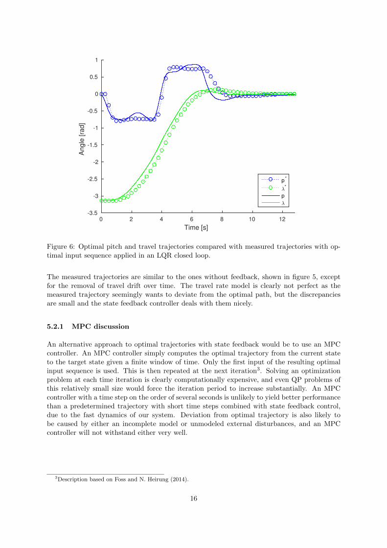
Figure 6: Optimal pitch and travel trajectories compared with measured trajectories with op-timal input sequence applied in an LQR closed loop.

The measured trajectories are similar to the ones without feedback, shown in figure 5, exceptfor the removal of travel drift over time. The travel rate model is clearly not perfect as themeasured trajectory seemingly wants to deviate from the optimal path, but the discrepanciesare small and the state feedback controller deals with them nicely.

5.2.1 MPC discussion

An alternative approach to optimal trajectories with state feedback would be to use an MPCcontroller. An MPC controller simply computes the optimal trajectory from the current stateto the target state given a finite window of time. Only the first input of the resulting optimalinput sequence is used. This is then repeated at the next iteration3. Solving an optimizationproblem at each time iteration is clearly computationally expensive, and even QP problems ofthis relatively small size would force the iteration period to increase substantially. An MPCcontroller with a time step on the order of several seconds is unlikely to yield better performancethan a predetermined trajectory with short time steps combined with state feedback control,due to the fast dynamics of our system. Deviation from optimal trajectory is also likely tobe caused by either an incomplete model or unmodeled external disturbances, and an MPCcontroller will not withstand either very well.

3Description based on Foss and N. Heirung (2014).

16

6 Optimal Control of Pitch/Travel and Elevation with and with-out Feedback

6.1 State space model

Adding e and e to the previous state space model (4) using (3b), we get

λ

λppee

=

0 1 0 0 0 00 −0.03 −0.39 0 0 00 0 0 1 0 00 0 −7.13 −3.6 0 00 0 0 0 0 10 0 0 0 −3.03 −2.44

︸︷︷︸

Ac

λ

λppee

+

0 00 00 0

6.74 00 00 3.13

︸︷︷︸

Bc

[pcec

]. (12)

The added states are clearly decoupled from the rest of the system. This is due to the factthat the model is linearized around the equilibrium. At small pitch angles this simplificationdoes not cause any large discrepancies. However, when the pitch angle is large, an increase inelevation rate is clearly accompanied by an increase in travel rate.

6.2 Discretization

Now let x =[λ λ p p e e

]>, u =

[pc ec

]>. Again, using approximate discretization via

the Euler method we obtain a discrete state space model

xk+1 = (I + ∆tAc)xk + (∆tBc)uk.

= Axk +Buk, (13)

where

A =

1 0.25 0 0 0 00 0.9925 −0.0975 0 0 00 0 1 0.25 0 00 0 −1.7825 0.1 0 00 0 0 0 1 0.250 0 0 0 −0.7575 0.39

, B =

0 00 00 0

1.685 00 00 0.7825

.

6.3 Optimization problem with nonlinear constraints

We calculate an optimal trajectory from x0 =[λ0 0 0 0 0 0

]>to xf =

[λf 0 0 0 0 0

]>minimizing the objective function

φ =N∑i=1

(λi − λf )2 + r1p2ci−1

+ r2e2ci−1

, r1, r2 ≥ 0,

or alternatively

φ =

N−1∑i=0

(xi+1 − xf )>Q(xi+1 − xf ) + u>i Rui, (14)

17

where

Q =

1 0 0 0 0 00 0 0 0 0 00 0 0 0 0 00 0 0 0 0 00 0 0 0 0 00 0 0 0 0 0

, R =

[r1 00 r2

]. (15)

The second weighting parameter r2 is added as an inequality constraint is imposed on theelevation for every time step:

c(xk) = α exp(−β (λk − λt)2

)− ek ≤ 0, k = {1, . . . , N}, (16)

where we let α = 0.2, β = 20, λt = 2π3 .

The objective function (14) is subject to the system dynamics (13) and thus imposed to linearequality constraints identically defined to that of (8). Similarly to (9) we define the optimizationvariable z and the matrix G, and the resulting optimization problem can be stated:

minz

zTGz (17a)

subject to

Aeqz = Beq, (17b)

c(xk) ≤ 0, k = {1, . . . N}, (17c)

plow ≤ pk, pck−1≤ phigh, k = {1, . . . N}. (17d)

(17e)

6.4 Discrete-time LQR

In addition to running the optimal input sequence u∗ in an open loop, a discrete-time LQR asdefined in 5.1 is applied, with the weigthing matrices

Q =

4 0 0 0 0 00 2 0 0 0 00 0 0 0 0 00 0 0 0 0 00 0 0 0 3 00 0 0 0 0 0

, R =

[1 00 1

]. (18)

6.5 Optional: Additional constraints

Although the calculated input yielded satisfactory performance, the model has shortcomings.Specifically, when a slwe impose ow descent in elevation is commanded the rotor blades almostcome to a complete stop, during which control of pitch is severely reduced. As this is impossibleto model with a linear model, additional bounds are imposed on elevation rate. This will reduce

18

the effect of the unmodeled coupling of elevation to the rest of the system. In a further attemptto keep the system within the linear area the travel rate is also bounded:

−0.05 ≤ ek ≤ 0.05, k = {1, . . . N},−0.5 ≤ λk ≤ 0.5, k = {1, . . . N}.


Because of the non-linearity of (16) it is no longer viable to use a QP-solver, and (17) is solvedusing MATLAB’s fmincon using an active set method. The pitch bounds are also tightenedfrom 45◦ to 25◦ in order to lower the effect of elevation rate and travel rate coupling at largepitch angles.

The optimal input sequence u∗ is applied to the plant in an open loop with results shown infigure 7. The system follows the optimal trajectory except for the usual discrepancy in travelpresent when using open loop control. We further employ the LQR to guide the trajectory tothe set-point and eliminate steady state deviations. The result, shown in figure 8, is withoutany large discrepancies between optimal and measured trajectory. However, the constraintbound imposed on elevation is violated, as shown in figure 10. The reason for this is probably acombination of issues. The optimal path is calculated with a fairly large time step, in order tolower the computational time required. This leads to an optimal path that when interpolatedwill violate the constraint. Also, as the increase in elevation will largely happen when the pitchangle is at its maximum, and the resulting increase in elevation will be lower than if the increasewere to be commanded at zero pitch. State feedback is also unable to deal with this problemcompletely, as any aggressive elevation correction is bound to happen at the cost of pitch, andtherefore travel rate control. Lastly, the trajectory is corrected with respect to the optimalpath in time, while the bound on elevation is defined with respect to travel. This means thata deviation in travel, as visible in figure 8, effectively will shift the optimal elevation path withrespect to travel. This lag is visible in figure 10.

The mentioned effects contributing to constraint violation are attempted minimized by theaddition of extra constraints on elevation rate and travel rate, as mentioned in 6.5. The resultingoptimal path reflects this, and the slope of the optimal elevation path is significantly reduced.This yields an overall less aggressive system, with decreased violation of the elevation constraint.The added constraint on travel rate also means that the system uses the entire time slot to reachthe desired end state.

19

Time [s]

0 2 4 6 8 10 12

Angle

[ra

d]

-3.5

-3

-2.5

-2

-1.5

-1

-0.5

0

0.5

p

λ

e

p*

λ*

e*

Figure 7: Optimal pitch, travel and elevation trajectories compared with measured trajectories,with optimal input sequence applied in an open loop.

Time [s]

0 2 4 6 8 10 12

Angle

[ra

d]

-3.5

-3

-2.5

-2

-1.5

-1

-0.5

0

0.5

1

p

λ

e

p*

λ*

e*

Figure 8: Optimal pitch, travel and elevation trajectories compared with measured trajectories,with optimal input sequence applied in an LQR closed loop.

20

Time [s]

0 2 4 6 8 10 12

Angle

[ra

d]

-3.5

-3

-2.5

-2

-1.5

-1

-0.5

0

0.5

p

λ

e

p*

λ*

e*

Figure 9: Optimal trajectories compared with closed loop measured trajectories, with lower andupper bounds added to elevation rate and travel rate.

Travel [rad]

-3 -2.5 -2 -1.5 -1 -0.5 0

Ele

vation [ra

d]

-0.05

0

0.05

0.1

0.15

0.2

c

e

e*

Figure 10: Inequality contraint imposed on elevation compared with the optimal and measuredtrajectories, with LQR.

21

Travel [rad]

-3 -2.5 -2 -1.5 -1 -0.5 0

Ele

vation [ra

d]

-0.05

0

0.05

0.1

0.15

0.2

c

e

e*

Figure 11: Inequality contraint imposed on elevation compared with the optimal and measuredtrajectories, with additional lower and upper bounds on elevation rate and travel rate.

22

7 Discussion

The optimal paths computed have shown to be quite compatible with the actual system. Thisis reflected in the displayed data. The reason for discrepancies have also been relatively easy toidentify. This is probably due to mainly two related facts. The controllers of pitch and elevationwere tuned in a way that gave the least nonlinear coupling between them. This greatly improvesthe changes of a linear model being sufficient. Secondly, the statistically system identificationyields a model with an accuracy far greater than one based on indirect measurements. Optimalpaths based on an incomplete system model will probably yield suboptimal performance at best.

As shown in both figure 5 and 7 the need for feedback control is present. A linear quadraticcontroller is a computationally inexpensive way of achieving this. The feedback importance isalso reduced by having an accurate system model, and only light corrections were necessary.

The effect of model shortcomings as discussed in 3.3, 4.1, 6.1, 6.5 and 6.6 are attempted min-imized by adding extra constraints to the optimization problem. This forces the system tooperate inside the linear area, yielding slower but more accurate performance.

23

8 Conclusion

Optimal operation of the movable arm is achieved by minimizing a quadratic cost function, andprecomputed input sequences are supplemented by state feedback. The linear model is shownto yield satisfactory performance, and enhanced performance is achieved by adding constraintsdesigned to minimize nonlinear effects.

24

A MATLAB Scripts

A.1 Controller tuning and model parameter estimation

1 clear all; close all; clc2

3 %% Pitch4 % h = pitch/pitch_ref5

6 load pitchStep40deg7 u_pitch = 40*pi/180 * ones(3000,1);8 u_pitch(1) = 0;9 y_pitch = pitchStep40deg.signals.values(1:3000);

10 pitch_data = iddata(y_pitch, u_pitch, 0.001);11 pitch_time = 0.001:0.001:3;12

13 opt = tfestOptions(’InitialCondition’, ’zero’);14 pitch_sys = tfest(pitch_data, 2, 0,opt); % poles, zeroes15

16 %% Elevation17 % h = elevation/elevation_ref18

19 load elevStep30deg20 u_elev = 30*pi/180 * ones(7000,1);21 u_elev(1) = 0;22 y_elev = elevStep30deg.signals.values(1:7000) + 16.8*pi/180; % unbias the step23 elev_data = iddata(y_elev, u_elev, 0.001);24 elev_time = 0.001:0.001:7;25

26 opt = tfestOptions(’InitialCondition’, ’zero’);27 elev_sys = tfest(elev_data, 2, 0,opt); % poles, zeroes28

29 %% TravelRate30 % h = travelRate/pitch31

32 load travelRateStep20deg33 travelRate_time = 0.001:0.001:8;34 u_travelRate = 20*pi/180 * step(pitch_sys,travelRate_time);35 y_travelRate = travelRateStep20deg.signals.values(1:8000) - 0.02; % unbias36 travelRate_data = iddata(y_travelRate, u_travelRate, 0.001);37

38 opt = tfestOptions(’InitMethod’,’iv’,’InitialCondition’, ’zero’);39 travelRate_sys = tfest(travelRate_data, 1, 0, opt); % poles, zeroes

A.2 Optimal control of pitch/travel without feedback

1 clear all; close all; clc2 init023

4 %% Continuous model5 Ac = [0 1 0 0;6 0 -0.03 -0.39 0;7 0 0 0 1;8 0 0 -7.13 -3.6];9 Bc = [ 0 0 0 6.74]’;

10

11 %% Discrete model12 dt = 0.25;13 A = eye(4) + Ac*dt;

25

14 B = Bc*dt;15

16 % given: x0 = [0 0 0 0]’;17 xf = [pi 0 0 0]’;18

19 n_x = size(A,2);20 n_u = size(B,2);21

22 %% Simulatin parameters23 duration = 25;24 N = floor(duration/dt);25 r = .1;26 pitch_lim = 45; % deg27

28 %% Equality constraints29

30 Aeq = [ eye(N*n_x) + kron(diag(ones(N-1,1),-1), -A) , kron(eye(N), -B)];31

32 beq = [-A*xf;33 zeros(n_x*(N-1),1)];34

35 %% Bounds36 LB_x = repmat([-Inf -Inf -pitch_lim*pi/180 -Inf]’, N, 1);37 UB_x = repmat([Inf Inf pitch_lim*pi/180 Inf]’, N, 1);38

39 LB_u = repmat(-pitch_lim*pi/180, N, 1);40 UB_u = repmat(pitch_lim*pi/180, N, 1);41

42 LB = [LB_x;43 LB_u];44

45 UB = [UB_x;46 UB_u];47

48 %% Quadratic objective function49 Q = zeros(n_x);50 Q(1,1) = 1;51

52 R = r;53

54 G = blkdiag(kron(eye(N), Q), kron(eye(N), R));55

56 %% Solve QP57 [z,fval,exitflag,output,lambda] = quadprog(G, [], [], [], Aeq, beq, LB, UB);58

59 x = reshape(z(1:N*n_x), [n_x, N]);60 travel_opt = [-xf(1), x(1,:)];61 pitch_opt = [-xf(3), x(3,:)];62 u = [reshape(z(N*n_x+1:end), [n_u, N]) , zeros(n_u, 1)];63

64 %% Prep input sequence65 padding_time = 10;66 padded_input = [zeros(1,floor(padding_time/dt)) , u]’;67 time = [(0:length(padded_input) - 1)*dt]’;68 heli_input = [time padded_input];

A.3 Optimal control of pitch/travel with feedback (LQ)

1 %% LQR2 Q = diag([4,2,0,0]);

26

3 R = 0.1;4 K = dlqr(A,B,Q,R);5

6 %% Prep reference trajectory7 x_opt = x + repmat(xf, 1, length(x)); % Shift travel ref by pi8 padded_x_opt = [zeros(4,floor(padding_time/dt)) , x_opt];9 time = [(0:length(padded_x_opt) - 1)*dt];

10 heli_ref = [time; padded_x_opt]’;

A.4 Optimal control of pitch/travel and elevation with and without feedback

1 clear all; close all; clc2 init023

4 %% Continuous model5 Ac = [0 1 0 0 0 0;6 0 -0.03 -0.39 0 0 0;7 0 0 0 1 0 0;8 0 0 -7.13 -3.6 0 0;9 0 0 0 0 0 1;

10 0 0 0 0 -3.03 -2.44];11

12 Bc = [ 0 0;13 0 0;14 0 0;15 6.74 0;16 0 0;17 0 3.13];18

19 %% Discrete model20 dt = .25;21 A = eye(6) + Ac*dt;22 B = Bc*dt;23

24 % given: x0 = [0 0 0 0 0 0]’;25 xf = [pi 0 0 0 0 0]’;26

27 n_x = size(A,2);28 n_u = size(B,2);29

30 %% Simulation parameters31 duration = 12;32 N = floor(duration/dt);33 r1 = .1;34 r2 = .1;35 pitch_lim = 25; % deg36 elev_lim = 50;37 elev_rate_lim = 0.05; % Inf38 travel_rate_lim = 0.5; % Inf39

40 %% Equality constraints41

42 Aeq = [ eye(N*n_x) + kron(diag(ones(N-1,1),-1), -A) , kron(eye(N), -B)];43

44 Beq = [-A*xf;45 zeros(n_x*(N-1),1)];46

47 %% Bounds48 LB_x=repmat([-Inf -travel_rate_lim -pitch_lim*pi/180 -Inf -elev_lim*pi/180 -elev_rate_lim ]’,N,1);49 UB_x=repmat([Inf travel_rate_lim pitch_lim*pi/180 Inf elev_lim*pi/180 elev_rate_lim]’,N,1);

27

50

51 LB_u = repmat([-pitch_lim*pi/180 -elev_lim*pi/180]’, N, 1);52 UB_u = repmat([pitch_lim*pi/180 elev_lim*pi/180]’, N, 1);53

54 LB = [LB_x;55 LB_u];56

57 UB = [UB_x;58 UB_u];59

60

61 %% Quadratic objective function62 Q = zeros(n_x);63 Q(1,1) = 1;64

65 R = [r1 0;66 0 r2];67

68 G = blkdiag(kron(eye(N), Q), kron(eye(N), R));69

70 f = @(X) X’*G*X;71

72 %% Solve optimization problem73 tic74 [X, FVAL, EXITFLAG] = fmincon(f, zeros(N*8,1), [], [], Aeq, Beq, LB, UB, @constraint);75 toc76

77 x = reshape(X(1:N*n_x), [n_x, N]);78 travel_opt = [-xf(1), x(1,:)];79 pitch_opt = [-xf(3), x(3,:)];80 elevation_opt = [-xf(5), x(5,:)];81 u = [reshape(X(N*n_x+1:end), [n_u, N]) , zeros(n_u, 2)];82

83 %% LQR84 Q = diag([4,2,0,0,3,0]);85 R = diag([1 1]);86

87 K = dlqr(A,B,Q,R); % Closed loop88 %K = zeros(2,6); % Open loop89

90 %% Prep input sequence91 padding_time = 10;92 padded_input = [zeros(2,floor(padding_time/dt)) , u]’;93 time = [(0:length(padded_input) - 1)*dt]’;94 heli_input = [time padded_input];95

96 %% Prep reference trajectory97 x_opt = x + repmat(xf, 1, length(x)); % Shift travel ref by pi98 padded_x_opt = [zeros(6,floor(padding_time/dt)) , x_opt];99 time = (0:length(padded_x_opt) - 1)*dt;

100 heli_ref = [time; padded_x_opt]’;

28

B Simulink Diagrams

-C-

pitch

-C-

elevation

V_d

V_s

V_f

V_b

V_d/V_s --> V_f/V_b

data

To File

Terminator1Terminator

Step

p_c, rad

p, rad

p_dot, rad/sek

Out2

Pitch-kontroller

V_f, motor foran

V_b, motor bak

Vandring, (grader)

Vandringsrate, (grader/sek)

Pitch, (grader)

Pitchrate, (grader/sek)

Elevasjon, (grader)

Elevasjonsrate (grader/sek)

Heli 3D

e, rad

e_dot, rad/sek

e_c, rad

V_s

Elevasjonskontroller

D2R

Degrees toRadians

u-30

Bias

Figure 12: Simulink model used in section 3.

-C-

Zero1

V_d

V_s

V_f

V_b

V_d/V_s --> V_f/V_b

data.mat

To File

p_c, rad

p, rad

p_dot, rad/sek

Out2

Pitch-kontroller

V_f, motor foran

V_b, motor bak

Vandring, (grader)


Pitch, (grader)


Elevasjon, (grader)


Heli 3D

heli_input

FromWorkspace

e, rad

e_dot, rad/sek

e_c, rad

V_s


u-4

Bias1

u-30

Bias

D2R

D2R

D2R


29

-C-

Zero1

V_d

V_s

V_f

V_b

V_d/V_s --> V_f/V_b

data.mat

To File

Terminator1

Terminatorp_c, rad

p, rad

p_dot, rad/sek

Out2

Pitch-kontroller

V_f, motor foran

V_b, motor bak

Vandring, (grader)


Pitch, (grader)


Elevasjon, (grader)


Heli 3D

K*u

Gain

heli_ref

FromWorkspace1

heli_input

FromWorkspace

e, rad

e_dot, rad/sek

e_c, rad

V_s


u-4

Bias1

u-30

Bias

D2R

D2R

D2R


V_d

V_s

V_f

V_b

V_d/V_s --> V_f/V_b

data.mat

To File

p_c, rad

p, rad

p_dot, rad/sek

Out2

Pitch-kontroller

V_f, motor foran

V_b, motor bak

Vandring, (grader)


Pitch, (grader)


Elevasjon, (grader)


Heli 3D

K*u

Gain

heli_ref

FromWorkspace1

heli_input

FromWorkspace

e, rad

e_dot, rad/sek

e_c, rad

V_s


D2R

Degrees toRadians2

u-4

Bias1

u-30

Bias

D2R

1

D2R

D2R


30

Bibliography

Egeland, O. and Gravdahl, T. (2003). Modeling and Simulation for Automatic Control. MarineCybernetics.

Foss, B. and N. Heirung, T. A. (2014). Merging optimization and control.

Kwakernaak, H. and Sivan, R. (1972). Linear Optimal Control Systems. First Edition. Wiley-Interscience.

31

TTK4135 Optimization and Control Helicopter Lab Report€¦ · · 2015-04-29TTK4135 Optimization...

Documents

Transcript of TTK4135 Optimization and Control Helicopter Lab Report€¦ · · 2015-04-29TTK4135 Optimization...