Trust Region Superposition Methods for Protein Alignment ∗

R. Andreani † J. M. Martınez ‡ L. Martınez §

June 7, 2007

Abstract

Protein Alignment is a challenging applied Optimization problem. Superposition meth-ods are based on the maximization of a score function with respect to rigid-body modi-fications of relative positions. The problem of score maximization can be modeled as acontinuous nonsmooth optimization problem (LOVO). This allows one to define practicaland convergent methods that produce monotone increase of the score. In this paper, trustregion methods are introduced for solving the problem. Numerical results are presented.Computer software related to the LOVO approach for Protein Alignment is available inwww.ime.unicamp.br/∼martinez/lovoalign.

1 Introduction

Proteins are large organic compounds formed by chains of α-amino acids bound by peptidebonds. They are essential parts of all living organisms and participate in most cellular processes.Hormone recognition and transport, catalysis, transcription regulation, photosynthesis, cellularrespiration, and many other fundamental mechanisms of life are protein-mediated. Proteins canwork together to achieve a particular function, and can bind to different chemical structures tobe functional [42].

The sequence of amino acids in a protein is defined by a gene. This sequence is known asthe Primary Structure of a protein. Each amino acid has particular chemical characteristics,but contributes to the main chain of the protein with identical substructures formed by onenitrogen and two carbon atoms. One of these carbon atoms is known as the Cα atom. Roughlyspeaking, the 3D coordinates of the Cα atoms is known as the Tertiary Structure of a protein.Protein structures can be determined by experimental methods, such as X-ray crystallographyor Nuclear Magnetic Resonance. A large collection containing atom coordinates for most known

∗This work was supported by PRONEX-Optimization 76.79.1008-00, FAPESP (Grants 06/53768-0, 05/56773-1and 02-14203-6 ) and PRONEX CNPq/ FAPERJ 26/171.164/2003-APQ1. This paper is based on the talk givenby J. M. Martınez at the International Conference on Numerical Analysis and Optimization, held in Beijing, anddedicated to the 70th birthday of Prof. M. J. D. Powell in September 2006.

†Department of Applied Mathematics, IMECC-UNICAMP, State University of Campinas, CP 6065, 13081-970Campinas SP, Brazil. E-mail: andreani@ime.unicamp.br

‡Department of Applied Mathematics, IMECC-UNICAMP, State University of Campinas, CP 6065, 13081-970Campinas SP, Brazil. E-mail: martinez@ime.unicamp.br

§Institute of Chemistry, State University of Campinas. E-mail: lmartinez@iqm.unicamp.br.

1

proteins is the Protein Data Bank (PDB) [6], which contains around 35000 structures. Thisnumber increases every year.

During evolution, mutations promote changes in the primary structure of a protein by intro-ducing modifications in the genetic code. These mutations may persist in a population if theydo not result in impaired protein function. The function of different proteins may be the samein spite of different sequences of amino acids when they share the same overall three dimensionalstructure. Therefore, the classification of 3D structures is useful to determine the function ofthe proteins and to provide hints on evolutionary mechanisms.

The main ingredient of the classification procedure is the comparison (alignment) betweentwo structures. When a new protein structure is obtained, or when a protein structure isconjectured, its comparison with the whole data bank and consequent classification is oftenused for functional classifications [14].

The degree of similarity between two proteins is usually given by a score. From this score,a distance-like function is usually derived and the set of distances is frequently used to producestructure maps. A structure map is a 2D or 3D representation of the whole space of proteins [15].In a structure map, each protein is a point and the distance between two of these points reflectsthe similarity given by the score. Multidimensional scaling [16, 17, 41] and Kernel methods [28]are useful tools for building the 3D representation that comes from scores. The Structure SpaceMap developed in [16, 17] provides good predictions of function similarities in many cases.

The primary sequence of amino acids determines the structure of a protein. Protein foldingis the molecular mechanism by which a protein achieves its tertiary structure from an unfoldedsequence. Some general aspects of protein folding mechanisms are now being elucidated [35], butthe prediction of structure from sequence remains one of the greatest challenges of contemporarybiochemistry. Methods for structural modeling based on the sequence of amino acids exist,and are frequently based on sequence similarities with proteins with known structure. Theevaluation of the quality of the models requires a measure of their potential energy and of theirsimilarity with the structural references used [37]. Therefore, a score must be a reliable measureof similarity not only between known structures but also between potential ones.

We will see that the score that measures the similarity between two proteins may be seenas the maximum of a (continuous-nonsmooth) function in the space of relative positions (dis-placements). The reliability of the score depends on the accuracy in which we are able to obtainthis maximum, therefore robust and fast algorithms are necessary. Algorithms for obtaining theglobal maximum may be defined but are not affordable for the present computer facilities [23].

In this paper we rely on the mathematical characterization of the Protein Alignment problemgiven in [2] (see, also, [4]). Line-search algorithms that converge to first-order stationary pointswere defined in [2, 4]. Here we introduce a trust region approach [7, 29, 36] to define second-orderconvergent algorithms.

This paper is organized as follows. In Section 2, the Protein Alignment problem is formulatedas a Low Order Value Optimization problem. In Section 3 we define a trust region method forsolving LOVO and we prove convergence. In Section 4 we present numerical results. Conclusionsare given in Section 5.

NotationThe symbol ‖ · ‖ will denote the Euclidean norm.

2

If the symmetric matrix A is positive semidefinite, we denote A < 0. Analogously, if A ispositive definite, we denote A � 0.

We denote IN = {0, 1, 2, . . .}.The Euclidean ball with center x and radius ε is denoted B(x, ε).

2 Formulation

Let Q = {Q1, . . . , QN} ⊂ IRnq , P = {P1, . . . , PM} ⊂ IRnp . The goal is to find a transformationD : IRnq → IRnp such that some subset of {D(Q1), . . . , D(QN )} fits some subset of P. In ProteinAlignment, D generally represents rigid-body displacements but more general transformationscan be considered. For example, assume that nq = 3, np = 2 and that P is the set of possible“shadows” of the points in Q. In that case, one could wish to find the rigid-body displacement ofQ such that a subset of the two-dimensional points represented by the (x, y) coordinates of thedisplaced Q fits a subset of P in the best possible way. In that case, D would be the compositionof a rigid-body movement with a projection. A lot of examples of this general problem can begiven, from tissue recognition to security systems [3]. We will denote D the set of admissibletransformations.

Let C be the set of admissible correspondences between nonempty subsets of {1, . . . , N} and{1, . . . ,M}. (Sometimes, admissible correspondences must be bijective, sometimes monotonicitywill be required.)

Each element Φ ∈ C is a functionΦ : A→ B,

where A ⊂ {1, . . . , N} and B ⊂ {1, . . . ,M}. Given Φ ∈ C and a transformation D, an associatedscore S(D,Φ) ≥ 0 is assumed to be defined. This score should reflect the degree of spatialsimilarity between the sets {D(Qa)}a∈A and {Pb}b∈B.

The goal of the general alignment problem is to maximize, both with respect to Φ and withrespect to D, the score S(D,Φ). In other words, we wish to solve the problem:

MaximizeD∈D MaximumΦ∈C S(D,Φ). (1)

Since C is a finite set (say, C = {Φ1, . . . ,Φm}) we may write (1) in the form

MaximizeD∈D Maximum {S(D,Φ1), . . . , S(D,Φm)}. (2)

Protein Alignment is a particular case of the situation explained above. The goal is to findsimilarities between two proteins P and Q, represented by the coordinates of their Cα atoms.The similarity is measured by a score. Several scores have been proposed in the protein literature.One of them is the Structal Score [13, 40]. Assume that the 3D-coordinates of the Cα atomsof protein P (in angstroms) are P1, . . . , PM and the coordinates of the Cα atoms of protein Qare Q1, . . . , QN . Under the rigid-body displacement D, the coordinates of the displaced proteinQ are, therefore, D(Q1), . . . , D(QN ). Assume that Φ is a monotone bijection between a subsetof {1, . . . , N} and a subset of {1, . . . ,M}. (We mean that i < j ⇒ Φ(i) < Φ(j).) The Structalscore associated to the displacement D and the bijection Φ is:

S(D,Φ) =∑ 20

1 + ‖Pk −D(QΦ(k))‖2/5,−10× gaps, (3)

3

Figure 1: Examples of correspondences that form the Φ domain: (a) Bijective correspondencesand (b) Non-bijective correspondences, valid only for NB methods.

where the∑

symbol involves the pairs (k,Φ(k)) defined by the bijection and gaps is the numberof cases in which at least one of the following situations occur:

• Φ(k) is defined, there exists ` > k such that Φ(`) is defined, but Φ(`+ 1) is not defined;

• Φ−1(k) is defined, there exists ` > k such that Φ−1(`) is defined, but Φ−1(` + 1) is notdefined.

In Figure 1 we give examples of bijective and nonbijective correspondences. The conceptof gap applies only to the bijective case. The bijection on the left has no gaps. The centralbijection has two gaps and the bijection on the right has one gap.

The Alignment Problem associated with the Structal score consists of finding Φ and D suchthat S(D,Φ) is maximal. A global optimization procedure for achieving this objective was givenin [23]. However, this method is not computationally affordable and, in practice, an heuristicprocedure called Structal Method [13, 40] is generally used. In [22], the Structal Method wasreported as the best available practical algorithm for protein alignment. Each iteration of theStructal Method consists of two steps:

1. Update Φ: Given the positions P1, . . . , PM and D(Q1), . . . , D(QN ), the monotone bijectionΦ that maximizes the score (fixing D) is computed using Dynamic Programming [33].

4

2. Update D: Assume that the graph of Φ is {(k1,Φ(k1)), . . . , (ks,Φ(ks))}. Then, the rigid-body displacement that minimizes

∑s`=1 ‖Pk`

−D(QΦ(k`))‖2 is computed.

The computation of D at the second step of the Structal Method involves the solution ofthe well known Procrustes problem [18, 19]. The main drawback of the Structal Method isthat the Update-Φ step aims the optimization of a function (the Structal score) with respect toΦ and the Update-D step involves the optimization of a different function (the sum of squareddistances) with respect to D. This may lead to oscillation [2].

The Structal Method is the most efficient Superposition method for Protein Alignment.Superposition methods are iterative algorithms whose main iteration has two phases:

1. Update Φ: Given the positions P1, . . . , PM and D(Q1), . . . , D(QN ), the admissible corre-spondence Φ that maximizes S (fixing D) is computed.

2. Update D: Assume that the graph of Φ is {(k1,Φ(k1)), . . . , (ks,Φ(ks))}. Then, a rigid-body displacement that presumably improves the score associated to this correspondenceis computed.

In [2] the set of admissible correspondences has been defined in two different ways: in the firstcase, an admissible correspondence must be a monotone bijection (as in the Structal Method)and, in the second case, admissible correspondences are mere functions between subsets of Qand P (bijective or not). The Structal score is used in both cases, but in the second case thegap-term is not included. In both cases, for a fixed correspondence Φ, the function S(D,Φ) isa continuous and smooth function of D. As a consequence, Protein Alignment methods thatimprove a score at every iteration are defined. The typical iteration of these methods has twophases, as in general superposition methods. The first phase is as stated above. In the secondphase we find a new displacement D that improves the score associated to Φ by means of acontinuous optimization method.

3 Low Order Value Optimization Algorithm

Assume that fi : IRn → IR, i = 1, . . . ,m. Define, for all x ∈ IRn,

fmin(x) = min{f1(x), . . . , fm(x)}.

We will consider the optimization problem

Minimize fmin(x). (4)

This is a Low Order Value optimization problem as defined in [3]. Let us identify the trans-formation D with the set of parameters by means of which D is defined (rotation angles andtranslation in the case of rigid-body displacements). Writing x = D, fi(x) = −S(D,Φi), weobserve that (2) is a particular case of (4). Therefore, the Protein Alignment problems definedin Section 2 are Order Value Optimization problems in the sense of (4). We will assume that thesecond derivatives of fi are Lipschitz-continuous on a sufficiently large set, for all i = 1, . . . ,m.This requirement is clearly fulfilled when S is the Structal score.

5

For all x ∈ IRn, we define:

Imin(x) = {i ∈ {1, . . . ,m} | fi(x) = fmin(x)}.

Here we will define a Newtonian trust region method for solving (4). This method will beapplied to the Protein Alignment problem.

Before defining the main algorithm, let us give a technical lemma, which will be useful bothin the well-definiteness proof and in the convergence proof.

Lemma 3.1. Let {xj} be a sequence that converges to x ∈ IRn and let f : IRn → IR possessLipschitz-continuous second derivatives on a open and convex set that contains {xj}. We defineψj, the second order quadratic approximation of f(x) by:

ψj(x) ≡ f(xj) +∇f(xj)T (x− xj) +12(x− xj)T∇2f(xj)(x− xj).

Assume that {∆j} is a sequence of positive numbers that tends to zero and define xj as a globalminimizer of ψj(x) subject to ‖x− xj‖ ≤ ∆j. Finally, assume that the condition

∇f(x) = 0 and ∇2f(x) < 0 (5)

does not hold, and define

ρj =f(xj)− f(xj)ψj(xj)− ψj(xj)

. (6)

Then,lim

j→∞ρj = 1.

Proof. Since x does not satisfy (5), we have that

∇f(x) 6= 0 (7)

or∇f(x) = 0 and ∇2f(x) 6< 0 . (8)

By the continuity of ∇f and the convergence of {xj}, if (7) takes place, we have that∇f(xj) 6= 0 for j large enough. In the case of (8), ∇2f(x) has a negative eigenvalue, therefore,∇2f(xj) 6< 0 for j large enough. Therefore, for j large enough, xj is not a solution of theproblem that defines xj . So, there exists j1 ∈ IN such that, for all j ≥ j1,

ψj(xj)− ψj(xj) < 0.

This implies that ρj is well defined (the denominator in (6) is not null) for j ≥ j1.Assume, first, that ∇f(x) 6= 0. Then, there exists d ∈ IRn be such that ‖d‖ = 1 and

∇f(x)Td < 0. (9)

Since ‖∆jd‖ = ∆j , for all j ≥ j1 we have:

6

ψj(xj) ≤ ψj(xj + ∆jd) = ψj(xj) + ∆j∇f(xj)Td+∆2

j

2dT∇2f(xj)d .

Therefore,

ψj(xj)− ψj(xj) ≤ ∆j∇f(xj)Td+‖∇2f(xj)‖ ∆2

j

2,

so,ψj(xj)− ψj(xj)

∆j≤ ∇f(xj)Td+

‖∇2f(xj)‖2

∆j .

Therefore, by (9) and the continuity of ∇f , there exists j2 ≥ j1 such that for all j ≥ j2,

ψj(xj)− ψj(xj)∆j

≤ ∇f(x)Td

2≡ a < 0. (10)

By Taylor’s theorem and (10), we have:

|ρj − 1| =∣∣∣∣f(xj)− f(xj)− [ψj(xj)− ψj(xj)]

ψj(xj)− ψj(xj)

∣∣∣∣ =∣∣∣∣ f(xj)− ψj(xj)ψj(xj)− ψj(xj)

∣∣∣∣=

∣∣∣∣∣f(xj)− f(xj)−∇f(xj)T (xj − xj)− 12(xj − xj)T∇2f(xj)(xj − xj)

ψj(xj)− ψj(xj)

∣∣∣∣∣≤ o(∆2

j )/(−a∆j)→ 0.

Therefore, limj→∞

ρj = 1.

Assume now that (8) holds. Then, there exists d ∈ IRn such that ‖d‖ = 1 and

dT∇2f(x)d < 0.

For all j ≥ j1, define dj = d if ∇f(xj)Td ≤ 0 and dj = −d if ∇f(xj)Td > 0.Since ‖∆jdj‖ = ∆j , we have:

ψj(xj) ≤ ψj(xj + ∆jdj) ≤ ψj(xj) +∆2

j

2dT

j ∇2f(xj)dj .

Therefore, since dTj ∇2f(xj)dj = dT∇2f(xj)d,

ψj(xj)− ψj(xj)∆2

j

≤ 12dT∇2f(xj)d.

Hence, by the continuity of ∇2f(x), there exists j3 ∈ IN such that for all j ≥ j3,

ψj(xj)− ψj(xj)∆2

j

≤ 14dT∇2f(x)d ≡ b < 0 . (11)

7

Therefore,

|ρj − 1| =∣∣∣∣ f(xj)− ψj(xj)ψj(xj)− ψj(xj)

∣∣∣∣ ≤ o(‖xj − xj‖2)∆2

j |b|≤o(∆2

j )∆2

j

→ 0.

Then, limj→∞

ρj = 1. This completes the proof. �

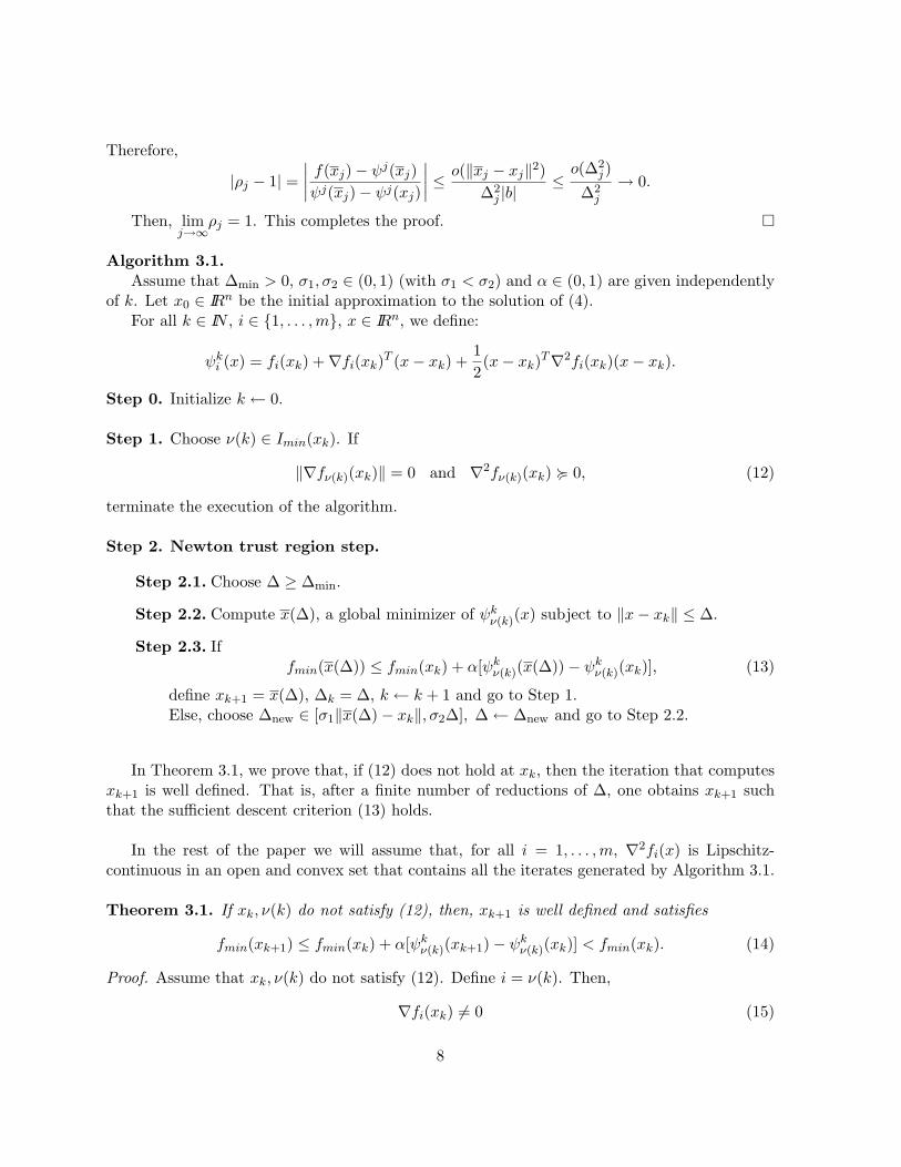
Algorithm 3.1.Assume that ∆min > 0, σ1, σ2 ∈ (0, 1) (with σ1 < σ2) and α ∈ (0, 1) are given independently

of k. Let x0 ∈ IRn be the initial approximation to the solution of (4).For all k ∈ IN , i ∈ {1, . . . ,m}, x ∈ IRn, we define:

ψki (x) = fi(xk) +∇fi(xk)T (x− xk) +

12(x− xk)T∇2fi(xk)(x− xk).

Step 0. Initialize k ← 0.

Step 1. Choose ν(k) ∈ Imin(xk). If

‖∇fν(k)(xk)‖ = 0 and ∇2fν(k)(xk) < 0, (12)

terminate the execution of the algorithm.

Step 2. Newton trust region step.

Step 2.1. Choose ∆ ≥ ∆min.

Step 2.2. Compute x(∆), a global minimizer of ψkν(k)(x) subject to ‖x− xk‖ ≤ ∆.

Step 2.3. Iffmin(x(∆)) ≤ fmin(xk) + α[ψk

ν(k)(x(∆))− ψkν(k)(xk)], (13)

define xk+1 = x(∆), ∆k = ∆, k ← k + 1 and go to Step 1.Else, choose ∆new ∈ [σ1‖x(∆)− xk‖, σ2∆], ∆← ∆new and go to Step 2.2.

In Theorem 3.1, we prove that, if (12) does not hold at xk, then the iteration that computesxk+1 is well defined. That is, after a finite number of reductions of ∆, one obtains xk+1 suchthat the sufficient descent criterion (13) holds.

In the rest of the paper we will assume that, for all i = 1, . . . ,m, ∇2fi(x) is Lipschitz-continuous in an open and convex set that contains all the iterates generated by Algorithm 3.1.

Theorem 3.1. If xk, ν(k) do not satisfy (12), then, xk+1 is well defined and satisfies

fmin(xk+1) ≤ fmin(xk) + α[ψkν(k)(xk+1)− ψk

ν(k)(xk)] < fmin(xk). (14)

Proof. Assume that xk, ν(k) do not satisfy (12). Define i = ν(k). Then,

∇fi(xk) 6= 0 (15)

8

or∇fi(xk) = 0 and ∇2fi(xk) 6< 0 . (16)

Observe thatψk

i (xk) = fi(xk) = fmin(xk). (17)

For all ∆ > 0, we define x(∆) as a minimizer of ψki (x) subject to ‖x − xk‖ ≤ ∆. By (15)

and (16), xk is not a minimizer of this subproblem.Define, for all ∆ > 0,

ρ(∆) =fi(x(∆))− fi(xk)ψk

i (x(∆))− ψki (xk)

.

By Lemma 3.1, if {∆j} is a sequence of positive numbers that tends to zero, we have that

limj→∞

ρ(∆j) = 1.

Therefore, lim∆→0

ρ(∆) = 1. Since fmin(x(∆)) ≤ fi(x(∆)), this implies that for ∆ sufficiently

small, (14) will be fulfilled. So, the proof is complete. �

Remark. Theorem 3.1 says that, if Algorithm 3.1 terminates at xk, then there exists i ∈Imin(xk) such that xk is a second-order stationary point of fi. The reciprocal is not true. Forexample, define, with n = 1,m = 2, f1(x) = x, f2(x) = x2. Clearly, 0 is a second order station-ary point of f2. However, if one chooses ν(k) = 1, the algorithm will not stop and, in fact, itwill find a better point such that fmin(x) < fmin(0).

Theorem 3.2 Assume that, for an infinite set of indices K ⊂ IN , we have that limk∈K = x∗,where {xk} is an infinite sequence generated by Algorithm 3.1. Then:

1. If i ∈ {1, . . . ,m} is such that ν(k) = i for infinitely many indices k ∈ K, then

∇fi(x∗) = 0 and ∇2fi(x∗) < 0. (18)

2. There exists i ∈ Imin(x∗) such that ∇fi(x∗) = 0 and ∇2fi(x∗) < 0.

Proof. The sequence {∆k}k∈K satisfies one of the following possibilities:

lim infk∈K

∆k = 0 (19)

or{∆k}k∈K is bounded away from 0. (20)

Assume, initially, that (19) holds. Then, there exists an infinite set of indices K1 ⊂ K suchthat

limk∈K1

∆k = 0 . (21)

9

Therefore, there exists k1 ∈ IN such that ∆k < ∆min for all k ∈ K2, whereK2 ≡ {k ∈ K1 | k ≥ k1}.Since, at each iteration, the initial trial trust region radius is greater than or equal to ∆min, itturns out that, for all k ∈ K2, there exist ∆k and x(∆k) such that x(∆k) is global solution of

Minimize ψki (x)

‖x− xk‖ ≤ ∆k(22)

butfi(x(∆k)) ≥ fmin(x(∆k)) > fi(xk) + α[ψk

i (x(∆k))− ψki (xk)] . (23)

Clearly, (22) implies that x(∆k) is global solution of:

Minimize ψki (x)

‖x− xk‖ ≤ ‖x(∆k)− xk‖.(24)

By the definition of ∆k at Step 2 of Algorithm 3.1, we have:

∆k > σ1 ‖x(∆k)− xk‖ . (25)

Therefore, by (21) e (25) we have that

limk∈K3

‖x(∆k)− xk‖ = 0 . (26)

Define

ρk =fi(x(∆k))− fi(xk)ψk

i (x(∆k))− ψki (xk)

. (27)

By Lemma 3.1, if (18) does not hold, we have that limk∈K2 ρk = 1, which contradicts (23).Therefore, (18) is proved in the case (19).

Let us consider the possibility (20). Since fmin(xk+1) ≤ fmin(xk) for all k, and limk∈K xk =x∗, by the continuity of fmin we have that limk→∞[fmin(xk+1) − fmin(xk)] = 0. Therefore, by(14),

limk∈K

(ψki (xk+1)− ψk

i (xk)) = 0 . (28)

Define ∆ = infk∈K1

∆k > 0 and let x be a global solution of

Minimize ∇fi(x∗)T (x− x∗) + 12(x− x∗)T∇2fi(x∗)(x− x∗)

‖x− x∗‖ ≤ ∆/2 .(29)

Let k3 ∈ IN such that‖xk − x∗‖ ≤ ∆/2 (30)

for all k ∈ K4 ≡ {k ∈ K | k ≥ k3}.By (29) and (30), for all k ∈ K4, we have:

‖x− xk‖ ≤ ∆ ≤ ∆k. (31)

10

Therefore, since xk+1 is a global minimizer of ψki (x) subject to ‖x− xk‖ ≤ ∆k, we get:

ψki (xk+1) ≤ ψk

i (x) = ψki (xk) +∇fi(xk)T (x− xk) +

12(x− xk)T∇2fi(xk)(x− xk). (32)

So,

ψki (xk+1)− ψk

i (xk) ≤ ∇fi(xk)T (x− xk) +12(x− xk)T∇2fi(xk)(x− xk) . (33)

By (28), taking limits in (33) for k ∈ K3, we have that:

0 ≤ ∇fi(x∗)T (x− x∗) +12(x− x∗)T∇2fi(x∗)(x− x∗).

Therefore x∗ is a global minimizer of (29) for which the constraint ‖x−x∗‖ < ∆/2 is inactive.This implies that ∇fi(x∗) = 0 and ∇2fi(x∗) < 0.

So, the first part of the thesis is proved.Now, let us prove the second part of the thesis. Since {1, . . . ,m} is finite, there exists

i ∈ {1, . . . ,m} such that i = ν(k) for infinitely many indices k ∈ K1 ⊂ K. So, for all k ∈ K1,

fi(xk) ≤ fj(xk) ∀ j ∈ {1, . . . ,m}.

Taking limits in the previous inequality and using the first part of the thesis, we get:

fi(x∗) ≤ fj(x∗) ∀ j ∈ {1, . . . ,m}.

Therefore, i ∈ Imin(x∗). �

Assumption A1. We say that this assumption holds at x∗ if, for all i ∈ Imin(x∗) such that∇fi(x∗) = 0, we have that ∇2fi(x∗) � 0.

Lemma 3.2. Assume that x∗ is a limit point of a sequence generated by Algorithm 3.1 and thatAssumption A1 holds at x∗. Then, there exists ε > 0 such that the reduced ball B(x∗, ε)− {x∗}does not contain limit points of {xk}.

Proof. If i ∈ Imin(x∗) and ∇fi(x∗) = 0, we have, by Assumption A1, that ∇2fi(x∗) is pos-itive definite. Therefore, by the Inverse Function Theorem, ∇fi(x) 6= 0 for all x 6= x∗ in aneighborhood of x∗.

If i ∈ Imin(x∗) and ∇fi(x∗) 6= 0, then ∇fi(x) 6= 0 in a neighborhood of x∗.Finally, if i /∈ Imin(x∗), we have that fi(x∗) > fmin(x∗). So, fi(x) > fmin(x) and i /∈ Imin(x)

for all x in a neighborhood of x∗.Therefore, there exists ε > 0 such that ∇fi(x) 6= 0 whenever i ∈ Imin(x) and x ∈ B(x∗, ε)−

{x∗}. Therefore, by Theorem 3.2, x cannot be a limit point of a sequence generated by Algo-rithm 3.1, for all x ∈ B(x∗, ε)− {x∗}. �

Lemma 3.3. Suppose that x∗ satisfies Assumption A1 and limk∈K xk = x∗, where {xk} is asequence generated by Algorithm 3.1 and K is an infinite subset of indices. Then,

limk∈K‖xk+1 − xk‖ = 0.

11

Proof. Let I be the set of integers in {1, . . . ,m} such that i = ν(k) for infinitely many indicesk ∈ K. Since fi(xk) = fmin(xk) infinitely many times, we obtain, taking limits, that i ∈ Imin(x∗)for all i ∈ I. Therefore, by Theorem 3.2, ∇fi(x∗) = 0 and, consequently, limk∈K ∇fi(xk) = 0for all k ∈ I. This implies that

limk∈K∇fν(k)(xk) = 0. (34)

Moreover, by Assumption A1, ∇2fi(xk) � 0 for all i ∈ I. So, by the continuity of the Hessians,there exists c > 0 such that, for all λ ≥ 0 and k ∈ K large enough:

‖[∇2fν(k)(x) + λI]−1‖ ≤ ‖∇2fν(k)(x)−1‖ ≤ 2 max

i∈I‖∇2fi(x∗)−1‖ = c. (35)

Now, xk+1 is a solution of

Minimize ψkν(k)(x) subject to ‖x− xk‖ ≤ ∆k (36)

Therefore, by the KKT conditions of (36),

(∇2fν(k)(xk) + λkI)(xk+1 − xk) +∇fν(k)(xk) = 0λk‖xk+1 − xk‖ = 0

λk ≥ 0, ‖xk+1 − xk‖ ≤ ∆k.(37)

Therefore, by (35), ‖xk+1 − xk‖ ≤ c‖∇fν(k)(xk)‖ for k ∈ K large enough, and, by (34),limk∈K ‖xk+1 − xk‖ = 0, as we wanted to prove. �

Theorem 3.3. Assume that x∗ is a limit point of a sequence {xk} generated by Algorithm 3.1.Suppose that Assumption A1 holds at x∗. Then, the whole sequence xk converges quadraticallyto x∗.

Proof. Let K be an infinite sequence of indices such that limk∈K xk = x∗. Let us prove first that

limk→∞

xk = x∗.

By Lemma 3.2, there exists ε > 0 such that x∗ is the unique limit point in the ball with centerx∗ and radius ε. Define

K1 = {k ∈ IN | ‖xk − x∗‖ ≤ ε/2}.

The subsequence {xk}k∈K1 converges to x∗, since x∗ is its unique possible limit point. Therefore,by Lemma 3.3,

limk∈K1

‖xk+1 − xk‖ = 0. (38)

Let k1 be such that, for all k ∈ K1, k ≥ k1,

‖xk+1 − xk‖ ≤ ε/2.

The set B(x∗, ε) − B(x∗, ε/2) does not contain limit points of {xk}. Therefore, there existsk2 ∈ IN such that, for all k ≥ k2,

‖xk − x∗‖ ≤ ε/2 or ‖xk − x∗‖ > ε.

12

Let k ∈ K1 such that k ≥ max{k1, k2}. Then,

‖xk+1 − x∗‖ ≤ ‖xk − x∗‖+ ‖xk+1 − xk‖ ≤ ε/2 + ε/2 = ε.

Since xk+1 cannot belong to B(x∗, ε)−B(x∗, ε/2), it turns out that ‖xk+1−x∗‖ ≤ ε/2. Therefore,k + 1 ∈ K1. So, we may prove by induction that x` ∈ K1 for all ` ≥ k. By (38), this impliesthat

limk→∞

xk = x∗. (39)

Let us prove now the quadratic convergence.Let I∞ ⊂ {1, . . . ,m} be the set of indices i such that i = ν(k) infinitely many times. Then,

there exists k2 such that for all k ≥ k2, ν(k) ∈ I∞.Now, if i ∈ I∞ it turns out that fi(xk) ≤ fmin(xk) infinitely many times. Therefore, by (39),

and the continuity of fi and fmin, we have that i ∈ Imin(x∗). By Theorem 3.2, ∇fi(x∗) = 0.Therefore, by Assumption A1,∇2fi(x∗) � 0. Thus, by the continuity of the Hessians, there existsci > 0 such that ∇2fi(x) is positive definite and ‖∇2fi(x)−1‖ ≤ ci for all x in a neighborhoodof x∗. This implies that there exists k3 ≥ k2 such that ∇2fν(k)(xk) is positive definite and‖∇2fν(k)(x)−1‖ ≤ β ≡ max{ci, i ∈ I∞} for all k ≥ k3.

Therefore, for all k ≥ k3, we may define

xk = xk −∇2fν(k)(xk)−1∇fν(k)(xk). (40)

Since ∇fi(x∗) = 0 for all i ∈ I∞, we have that limk→∞∇fν(k)(xk) = 0. Then, by theboundedness of ‖∇2fν(k)(x)−1‖, we have that ‖xk − xk‖ → 0, therefore, for k large enough,‖xk−xk‖ ≤ ∆min. But xk is, for k large enough, the unconstrained minimizer of ψk

ν(k). Therefore,since the first trust region radius at each iteration is greater than or equal to ∆min, it turns outthat, for k large enough, xk is the first trial point at each iteration of Algorithm 3.1.

By (40) we have that

|ψkν(k)(xk)− ψk

ν(k)(xk)| =12(xk − xk)T∇2fν(k)(xk)(xk − xk).

Therefore, by Assumption A1, there exists c > 0 such that for k large enough,

|ψkν(k)(xk)− ψk

ν(k)(xk)| ≥ c‖xk − xk‖2. (41)

Define

ρk =fν(k)(xk)− fν(k)(xk)ψk

ν(k)(xk)− ψki (xk)

By (41), and Taylor’s formula, we have that

|ρk − 1| =∣∣∣∣fi(xk)− fi(xk)− [ψk

i (xk)− ψki (xk)]

ψki (xk)− ψk

i (xk)

∣∣∣∣ ≤ o(‖xk − xk‖2)c‖xk − xk‖2

(42)

Since ‖xk − xk‖ → 0, we have that ρk → 1. Therefore, for k large enough, the sufficientdescent condition (14) is satisfied at the first trial point xk. Therefore, xk+1 = xk for k largeenough. This means that, for k ≥ k3 large enough,

xk+1 = xk −∇2fν(k)(xk)−1∇fν(k)(xk).

13

Then, by the elementary local convergence theory of Newton’s method (see, for example [8],pp. 90-91) we have that, for k large enough:

‖xk+1 − x∗‖ ≤ βγ‖xk − x∗‖2,

where γ is a Lipschitz constant for all the Hessians ∇2fi(x). �

4 Numerical results

Algorithm 3.1 was implemented with the following specifications:

1. We choose α = 0.1, σ1 = 0.001, σ2 = 5/9.

2. The initial ∆ at each iteration was chosen as the average norm of the Cα atoms of theprotein Q at their original positions multiplied by 10. This is a “big ∆” decision, theconsequence of which is that, in most iterations, the initial trial point comes from anunconstrained Newton step. Clearly, in Algorithm 3.1 we may consider that ∆min is equalto the adopted big ∆.

3. When (13) does not hold, ∆new is computed in the following way: We define

Ared = fmin(xk)− fmin(x),

P red = ψkν(k)(xk)− ψk

ν(k)(x),

and

∆new = max{

0.001,P red

2(Pred−Ared)

}× ‖x− xk‖. (43)

The fact that ∆new ≤ σ2‖x − xk‖ is guaranteed for σ2 = 5/9 because Ared > αPred inthe case that ∆new needs to be computed and α = 0.1 in our implementation.

We arrived to the formula (43) after careful experimentation with other possibilities, in-cluding the classical ones associated to smooth trust region methods (see, for example [10],pp. 95-96).

In order to optimize the behavior of Algorithm 3.1, it was crucial to define a “big” trustregion radius at the beginning of each iteration. The trust region radius that defines the firsttrial point was chosen to be independent of the last trust region radius employed at the previousiteration. This decision allowed the algorithm to use, very frequently, pure Newton steps andavoided artificial short steps far from the solution. Since the function fi that defines fmin at atrial point may be different than the one that defines fmin at the current point, the quadraticmodel of fmin tends to underestimate the true value in many cases. This fact seems to stimulatethe use of initial optimistic large steps.

We implemented Algorithm 3.1 under the framework of the standard trust region methodBetra for box-constrained optimization [5] (see www.ime.usp.br/∼egbirgin/tango). Sinceour problem is unconstrained, we set artificial bounds −1020, 1020 for each variable. The code

14

Betra needed to be adapted to the algorithmic decisions described at the beginning of thissection. In the unconstrained case, Betra is a standard trust region method that uses the More-Sorensen algorithm [30]. Many line-search and trust region methods for smooth unconstrainedminimization may be used for solving (4) if one simply ignores the nonsmoothness of the objectivefunction “defining” ∇fmin(x) = ∇fi(x) and ∇2fmin(x) = ∇2fi(x) for some i ∈ Imin(x). Ofcourse, the theoretical properties may change for each algorithmic choice. For example, wecannot expect that the thesis of Theorem 3.2 hold if one uses the algorithms TRON [26] orBOX-QUACAN [11] [26], since this theorem does not hold for those algorithms in the ordinarysmooth case (m = 1).

Numerical experiments were run on an AMD Opteron 242 with 1Gb of RAM running Linux.The software was compiled with the GNU fortran compiler version 3.3 with the “-O3 -ffast-math”options.

We employed two different versions of the trust region method for solving Protein Alignmentproblems:

1. Dynamic Programming Newton Trust (DP-Trust) method: Admissible correspondencesare monotone bijections between subsets of Q and P. This is the trust region counterpartof the line-search method DP-LS (Dynamic Programming Line-Search) introduced in [2].

2. Non-Bijective Newton Trust (NB-Trust) method: Admissible correspondences are, merely,functions (not necessarily bijective) between subsets of Q and P. This is the trust regioncounterpart of the line-search method NB-LS (Non-Bijective Line-Search) introduced in[2].

Given a rigid-body displacement D, the correspondence that maximizes the Structal Score(with gap penalization) is obtained using Dynamic Programming in DP-Trust, and using acheap procedure for computing non-bijective correspondences (described in [2, 4]) in NB-Trust(without gap penalization). The second phase at each iteration of DP-Trust and NB-Trust is aNewtonian trust region iteration as described in Section 3. The computer time of both methodsis dominated by the computation of the objective function. For DP-Trust, 98% of the time isspent on performing the dynamic programming steps and other 1.4% computing the gradient andthe hessian, which are steps also performed by the line-search procedure. For NB-Trust, the DPsteps required for obtaining the initial point and for computing the final Structal score takes 61%of the time, followed by the identification of the shortest distances (16%) and by the computationof the gradient and hessian of the objective function (15%). The cost of solving trust regionsubproblems represents less than 0.1% in both cases, thus being negligible. Therefore, it is notworthwhile to use approximate solutions of subproblems, instead of exact ones, as many wellestablished trust region methods for large-scale optimization do (see [7, 11, 26] and [34](Chapter4), among others).

We used the same initial approximations for the application of all the methods under con-sideration to Protein Alignment problems [2].

15

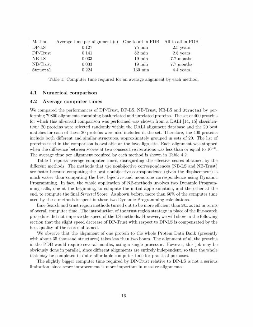
Method Average time per alignment (s) One-to-all in PDB All-to-all in PDBDP-LS 0.127 75 min 2.5 yearsDP-Trust 0.141 82 min 2.8 yearsNB-LS 0.033 19 min 7.7 monthsNB-Trust 0.033 19 min 7.7 monthsStructal 0.224 130 min 4.4 years

Table 1: Computer time required for an average alignment by each method.

4.1 Numerical comparison

4.2 Average computer times

We compared the performances of DP-Trust, DP-LS, NB-Trust, NB-LS and Structal by per-forming 79800 alignments containing both related and unrelated proteins. The set of 400 proteinsfor which this all-on-all comparison was performed was chosen from a DALI [14, 15] classifica-tion: 20 proteins were selected randomly within the DALI alignment database and the 20 bestmatches for each of these 20 proteins were also included in the set. Therefore, the 400 proteinsinclude both different and similar structures, approximately grouped in sets of 20. The list ofproteins used in the comparison is available at the lovoalign site. Each alignment was stoppedwhen the difference between scores at two consecutive iterations was less than or equal to 10−6.The average time per alignment required by each method is shown in Table 4.2.

Table 1 reports average computer times, disregarding the effective scores obtained by thedifferent methods. The methods that use nonbijective correspondences (NB-LS and NB-Trust)are faster because computing the best nonbijective correspondence (given the displacement) ismuch easier than computing the best bijective and monotone correspondence using DynamicProgramming. In fact, the whole application of NB-methods involves two Dynamic Program-ming calls, one at the beginning, to compute the initial approximation, and the other at theend, to compute the final Structal Score. As shown before, more than 60% of the computer timeused by these methods is spent in these two Dynamic Programming calculations.

Line Search and trust region methods turned out to be more efficient than Structal in termsof overall computer time. The introduction of the trust region strategy in place of the line-searchprocedure did not improve the speed of the LS methods. However, we will show in the followingsection that the slight speed decrease of DP-Trust with respect to DP-LS is compensated by thebest quality of the scores obtained.

We observe that the alignment of one protein to the whole Protein Data Bank (presentlywith about 35 thousand structures) takes less than two hours. The alignment of all the proteinsin the PDB would require several months, using a single processor. However, this job may beobviously done in parallel, since different alignments are entirely independent, so that the wholetask may be completed in quite affordable computer time for practical purposes.

The slightly bigger computer time required by DP-Trust relative to DP-LS is not a seriouslimitation, since score improvement is more important in massive alignments.

16

Figure 2: Performance profiles. (a) DP-Trust against DP-LS. (b) NB-Trust againts NB-LS. (c)DP-Trust against Structal. Analysis of the robustness of the methods for different alignmentqualities are shown in (d) and (e).

4.3 Performance Profiles

Performance profiles [9] concerning the comparison of the 5 methods are presented in this section.We consider that a method “solves” a problem when it obtains the best score up to a tolerance0.1%. If a method “does not solve” a problem, we consider, as usually, that the computer timeused is ∞. Given the abscissa x > 1, the profile curve of a method takes the value y if thereare y problems in which the computer time employed by this method is less than x times thecomputer time used by the best of the methods for the problem.

In Figure 2(a) the performance profile of DP-Trust against DP-LS is shown. DP-Trustobtains the best scores in 71% of the alignments, while DP-LS obtains the best scores in 67%.Therefore, the substitution of the line-search procedure by the trust region one improves therobustness of the alignment algorithm. Furthermore, for a relative time tolerance greater than2, DP-Trust appears to be more efficient than DP-LS.

There is no meaningful differences when we compare NB-Trust and NB-LS strategies, as

17

shown in Figure 2(b). In this set of alignments, NB-Trust obtains the best score (relatively onlyto these two methods) in 81% of the problems while NB-LS obtains best scores in 82% of thealignments. The differences in score values are not meaningful.

Finally, in order to contextualize the present results in terms of previously reported algo-rithms, we compute the performance profile of DP-Trust against Structal. DP-Trust is, asexpected, both faster and more robust than Structal, as shown in Figure 2(c).

4.4 Robustness and score relevance

Good protein alignment methods should be able to obtain the best possible scores. However, iftwo proteins are completely different, obtaining the best score is not so relevant. In practice,one is interested in giving accurate distances and identifying similarities only when the proteinsare similar.

With this in mind, we compared the scores obtained by each algorithm as a function of thebest score obtained. In other words, we want to compare the scores of different algorithms as afunction of the presumed protein similarity.

Figure 2(d) shows the percentage of cases in which each method was able to obtain thebest score (up to a relative precision of 10−3) as a function of the best score obtained for eachproblem. The best-Structal scores in the x−axis are normalized dividing by the number of atomsof the smallest protein being compared, so that normalized scores are between 0 and 20.

We observe that, for bad alignments, the Structal strategy is able to obtain the best scoresin the greatest number of cases, followed by DP methods and NB methods. However, for best-scores greater than only 2.5, DP-LS and DP-Trust methods obtain the best alignments morefrequently. For best-scores greater than 10 the best alignments are obtained by DP-Newtonmethods in more than 80% of the problems and, for best-scores greater than 13 this percentagegoes to more than 98%. Non-bijective algorithms fail to obtain the best scores for medium tobad alignments. However, for best-scores greater than 14, these methods also obtain the bestalignments, because the bijectivity of the best correspondence is automatically satisfied.

Figure 2(e) shows how close to the best score each method gets. The figure shows the averagescore obtained by each method relative to the best score obtained, as a function of the overallalignment quality. We can see, now, that the Structal Method obtains scores which are, onaverage, better than the ones obtained by NB methods. However, as shown in (Figure 2(d)),NB-methods obtain better scores than Structal for good alignments.

5 Final remarks

Protein Alignment is an challenging area for rigorous continuous Optimization. There is alot of space for the development of algorithms with well established convergent theories that,presumably, converge to local optimizers, and many times to global ones. We feel that line-search and Trust-Region methods for (1) are rather satisfactory, but different alternatives shouldbe mentioned. In [1], problems like (1) were reformulated as smooth nonlinear programmingproblems with complementarity constraints. This reformulation should be exploited in futureworks.

18

In this paper we showed that the trust region approach has some advantages over the line-search algorithm in terms of robustness, at least when one deals with DP-methods. We con-jecture that the advantages of trust region methods over line-search methods may be moreimpressive in other structural alignment problems. In particular, preliminary results for align-ments in which we allow internal rotations of the objects (see [4]) suggest that, in those cases,pure Newton directions are not so effective and restricted trust region steps could help. Furtherresearch is expected with respect to flexible alignments [25, 38, 43] in the near future.

In the experiments reported here, we always used the Structal score and we mentioned thefact that the Structal Method iteration maximizes this score at its first phase and minimizesthe sum of squared distances (RMSD) for the selected bijection at its second phase. This secondphase minimization admits an analytical solution [19]. Our approach here has been to maintainthe first phase (and the Structal Score) changing the second phase to preserve coherence. Theopposite choice is possible. We may preserve the Procrustes second phase, employing, at thefirst phase, a different score. An entirely compatible score with the Procrustes second phasemay be defined by:

S(D,Φ) = 20∑

max

[0, 1−

(‖Pk −D(QΦ(k))‖d0

)2]− 10× gaps,

where D,Φ,∑

and gaps are as in (3) and d0 is a threshold distance. If the distance betweentwo Cα atoms (associated by Φ) exceeds d0, its contribution to this score is zero. Maximizingthis score is equivalent to minimize the RMSD for the atoms for which di is less than d0. Threemethods based on different d0 values are also available in the LovoAlign software package.

We conjecture that the Low Order Value Optimization methodology may be employed inconnection to alignment and protein classification in a number of different related problems:conservation of residues in columns of a multiple sequence alignment [27], percentage identity[32], SVM detection of distant structural relationships [31], protein-protein interfacial residualidentification [24], prediction of subcellular localization [21], three-dimensional enzyme modeling[39], determination of score coefficients [20], hierarchical clustering [12] and many others.

AcknowledgementsThe authors are indebted to two anonymous referees, whose comments were very useful to

improve the presentation of the paper.

References

[1] R. Andreani, C. Dunder, and J. M. Martınez, Nonlinear-Programming Reformulation ofthe Order-Value Optimization problem, Mathematical Methods of Operations Research61, pp. 365-384 (2005).

[2] R. Andreani, J. M. Martınez, and L. Martınez, Convergent algorithms for protein struc-tural alignment, Technical Report, Department of Applied Mathematics, Unicamp, 2006.Currently available in the site www.ime.unicamp.br/∼martinez/lovoalign.

19

[3] R. Andreani, J. M. Martınez, L. Martınez, and F. Yano, Low Order Value Optimizationand Applications. Technical Report, Department of Applied Mathematics, Unicamp,2006. Currently available at www.ime.unicamp.br/∼martinez/lovoalign.

[4] R. Andreani, J. M. Martınez, L. Martınez, and F. Yano, Continuous Optimization Meth-ods for Structural Alignment, To appear in Mathematical Programming; 2007. Currentlyavailable at www.ime.unicamp.br/∼martinez/lovoalign.

[5] M. Andretta, E. G. Birgin and J. M. Martınez, Practical active set Euclidian trust-region method with spectral projected gradients for bound-constrained optimization,Optimization 54, pp. 305-325 (2005).

[6] H. M. Berman, et al., The Protein Data Bank, Nuclei Acids Research 17, pp. 235-242(2000).

[7] A. R. Conn, N. I. M. Gould, and Ph. L. Toint, Trust-Region Methods, MPS/SIAM Serieson Optimization, SIAM-MPS, Philadelphia, 2000.

[8] J. E. Dennis and R. B. Schnabel, Numerical Methods for Unconsconstrained Optimizationand Nonlinear Equations, Prentice-Hall, Englewood Cliffs, NJ, 1983. Reprinted by SIAMPublications, 1993.

[9] E. Dolan and J. J. More, Benchmarking optimization software with performance profiles,Mathematical Programming 91, pp. 201-213 (2002).

[10] R. Fletcher, Practical Methods of Optimization, John Wiley & Sons, New York, seconded., 1987.

[11] A. Friedlander, J. M. Martınez and S. A. Santos, A new trust region algorithm forbound constrained minimization, Applied Mathematics and Optimization 30, pp. 235-266 (1994).

[12] A. Gambin and P. R. Slonimski, Hierarchical clustering based upon contextual alignmentof proteins: a different way to approach phylogeny, Comptes Rendus Biologies 328, pp.11-22 (2005).

[13] M. Gerstein and M. Levitt, Comprehensive assessment of automatic structural alignmentagainst a manual standard, the Scop classification of proteins, Protein Sci. 7, pp. 445-456(1998).

[14] Holm, L., Sander C. Protein structure comparison by alignment of distance matrices. J.Mol. Biol. 1993;233:123-138.

[15] Holm, L, Sander, C. Mapping the Protein Universe. Science 1996;273:595–602.

[16] J. Hou, S.R. Jun, C. Zhang, and S. H. Kim, Global mapping of the protein structurespace and application in structure-based inference of protein function, P. Natl. Acad.Sci. USA 2006; 103: Early Edition.

20

[17] J. Hou, G. E. Sims, C. Zhang, and S. H. Kim, A global representation of the proteinfold space, P. Natl. Acad. Sci. USA 100, pp. 2386-2390 (2003).

[18] W. Kabsch, A discussion of the solution for the best rotation to relate two sets of vectors,Acta Crystallog. A 34, pp. 827-829 (1978).

[19] S. K. Kearsley, On the orthogonal transformation used for structural comparisons, ActaCrystallog. A 45, pp. 208-210 (1989).

[20] J. Kececioglu and E. Kim, Simple and fast inverse alignment, Research in ComputationalMolecular Biology, Proceedings Lecture Notes in Computer Science 3909, pp. 441-455(2006).

[21] J.K. Kim, G. P. S. Raghava, B. Y. Bang, and S. J. Choi, Prediction of subcellularlocalization of proteins using pairwise sequence alignment and support vector machine,Pattern Recognition Letters 27, pp. 996-1001 (2006).

[22] R. Kolodny, P. Koehl, and M. Levitt, Comprehensive evaluation of protein structurealignment methods: scoring by geometric measures, Journal of Molecular Biology 346,pp. 1173-1188 (2005).

[23] R. Kolodny and N. Linial, Approximate protein structural alignment in polynomial time.P. Natl. Acad. Sci. USA 101, pp. 12201-12206 (2004).

[24] J-J Li, D-S Huang, B. Wang, and P. Chen, Identifying protein-protein interfacial residuesin heterocomplexes using residue conservation scores, International Journal of BiologicalMacromolecules 38, pp. 241-247 (2006).

[25] Z-W Li, Y-Z Ye, and A. Godzik, Flexible structural neighborhood - a database of proteinstructural similarities and alignments, Nucleic Acids Research 34, D277-D280 (2006).

[26] C. Lin and J. J. More, Newton’s method for large bound-constrained optimization prob-lems, SIAM Journal on Optimization 9, pp. 1100-1127 (1999).

[27] X-S Liu, J. Li, W-L Guo, and W. Wang, A new method for quantifying residue conser-vation and its applications to the protein folding nucleus, Biochemical and BiophysicalResearch Communications 351, pp. 1031-1036 (2006).

[28] F. Lu, S. Keles, S. J. Wright, and G. Wahba, Framework for kernel regularization withapplication to protein clustering, P. Natl. Acad. Sci. USA 102, pp. 12332-12337 (2005).

[29] J. J. More, Recent developments in algorithms and software for trust region methods.In A. Bachem, M. Grotschel and B. Korte, eds., Mathematical Programming: The Stateof the Art pp. 258-287, Springer-Verlag, 1983.

[30] J. J. More and D. C. Sorensen, Computing a trust region step, SIAM Journal on Scien-tific and Statistical Computing 4, pp. 553-572 (1983).

21

[31] H. Ogul and E. U. Mumcuoglu, SVM-based detection of distant protein structural rela-tionships using pairwise probabilistic suffix trees, Computational Biology and Chemistry30, pp. 292-299 (2006).

[32] G. P. S. Raghava and G. J. Barton, Quantification of the variation in percentage identityfor protein sequence alignments, BMC Bioinformatics 7, Art 415 (2006).

[33] B. Needleman and C. D. Wunsch, A general method applicable to the search for simi-larities in the amino acid sequence of two proteins, Journal of Molecular Biology 48, pp.443-453 (1970).

[34] Nocedal J, Wright, SJ. Numerical Optimization, Springer 1999, New York.

[35] J. N. Onuchic and P. G. Wolynes, Theory of protein folding, Curr. Opin. Struct. Biol.2004;14:70-75.

[36] M. J. D. Powell, A new algorithm for unconstrained optimization. In J. B. Rosen, O. L.Mangasarian and K. Ritter, eds., Nonlinear Programming, pp. 31-65, Academic Press,1970.

[37] A. Sali, T. L. Blundell, Comparative protein modeling by satisfaction of spatial restraints.J. Mol. Biol. 234, 779-815, 1993.

[38] M. Shatsky, R. Nussinov, and H. J. Wolfson, Flexible protein alignment and hinge de-tection, Proteins 48 (2002) 242-256.

[39] N. Singh, G. Cheve, M. A. Avery, and C. R. McCurdy, Comparative protein modeling of1-deoxy-D-xylulose-5-phospate reductoisomerase enzyme from Plasmodium falciparum:A potential target for antimalarial drug discovery, Journal of Chemical Information andModeling 46, pp. 1360-1370 (2006)

[40] S. Subbiah, D. V. Laurents, and M. Levitt, Structural similarity of DNA-binding domainsof bacteriophage repressors and the globin core, Curr. Biol. 3, pp. 141-148 (1993).

[41] M. Vendruscolo and C. M. Dobson, A glimpse at the organization of the protein universe,P. Natl. Acad. Sci. USA 102, pp. 5641-5642 (2005).

[42] D. Voet and J. Voet, Biochemistry, John Wiley & Sons, 3d ed. 2004.

[43] Y-Z Ye and A. Godzik, Flexible structure alignment by chaining aligned fragment pairsallowing twists, Bioinformatics 19 (Suppl. 2) (2003) ii246-ii255.

22