Trust Region Policy Optimization - arXiv · parameterizations (Wampler & Popovi´c, 2009). The...

Trust Region Policy Optimization

John Schulman [email protected] Levine [email protected] Moritz [email protected] Jordan [email protected] Abbeel [email protected]

University of California, Berkeley, Department of Electrical Engineering and Computer Sciences

AbstractWe describe an iterative procedure for optimizingpolicies, with guaranteed monotonic improve-ment. By making several approximations to thetheoretically-justified procedure, we develop apractical algorithm, called Trust Region PolicyOptimization (TRPO). This algorithm is similarto natural policy gradient methods and is effec-tive for optimizing large nonlinear policies suchas neural networks. Our experiments demon-strate its robust performance on a wide varietyof tasks: learning simulated robotic swimming,hopping, and walking gaits; and playing Atarigames using images of the screen as input. De-spite its approximations that deviate from thetheory, TRPO tends to give monotonic improve-ment, with little tuning of hyperparameters.

1 IntroductionMost algorithms for policy optimization can be classifiedinto three broad categories: (1) policy iteration methods,which alternate between estimating the value function un-der the current policy and improving the policy (Bertsekas,2005); (2) policy gradient methods, which use an estima-tor of the gradient of the expected return (total reward) ob-tained from sample trajectories (Peters & Schaal, 2008a)(and which, as we later discuss, have a close connection topolicy iteration); and (3) derivative-free optimization meth-ods, such as the cross-entropy method (CEM) and covari-ance matrix adaptation (CMA), which treat the return as ablack box function to be optimized in terms of the policyparameters (Szita & Lorincz, 2006).

General derivative-free stochastic optimization methodssuch as CEM and CMA are preferred on many prob-lems, because they achieve good results while being sim-ple to understand and implement. For example, while

Proceedings of the 31 st International Conference on MachineLearning, Lille, France, 2015. JMLR: W&CP volume 37. Copy-right 2015 by the author(s).

Tetris is a classic benchmark problem for approximate dy-namic programming (ADP) methods, stochastic optimiza-tion methods are difficult to beat on this task (Gabillonet al., 2013). For continuous control problems, methodslike CMA have been successful at learning control poli-cies for challenging tasks like locomotion when providedwith hand-engineered policy classes with low-dimensionalparameterizations (Wampler & Popovic, 2009). The in-ability of ADP and gradient-based methods to consistentlybeat gradient-free random search is unsatisfying, sincegradient-based optimization algorithms enjoy much bettersample complexity guarantees than gradient-free methods(Nemirovski, 2005). Continuous gradient-based optimiza-tion has been very successful at learning function approxi-mators for supervised learning tasks with huge numbers ofparameters, and extending their success to reinforcementlearning would allow for efficient training of complex andpowerful policies.

In this article, we first prove that minimizing a certain sur-rogate objective function guarantees policy improvementwith non-trivial step sizes. Then we make a series of ap-proximations to the theoretically-justified algorithm, yield-ing a practical algorithm, which we call trust region pol-icy optimization (TRPO). We describe two variants of thisalgorithm: first, the single-path method, which can be ap-plied in the model-free setting; second, the vine method,which requires the system to be restored to particular states,which is typically only possible in simulation. These al-gorithms are scalable and can optimize nonlinear policieswith tens of thousands of parameters, which have previ-ously posed a major challenge for model-free policy search(Deisenroth et al., 2013). In our experiments, we show thatthe same TRPO methods can learn complex policies forswimming, hopping, and walking, as well as playing Atarigames directly from raw images.

2 PreliminariesConsider an infinite-horizon discounted Markov decisionprocess (MDP), defined by the tuple (S,A, P, r, ρ0, γ),where S is a finite set of states, A is a finite set of actions,P : S × A × S → R is the transition probability distri-

arX

iv:1

502.

0547

7v5

[cs

.LG

] 2

0 A

pr 2

017


bution, r : S → R is the reward function, ρ0 : S → R isthe distribution of the initial state s0, and γ ∈ (0, 1) is thediscount factor.

Let π denote a stochastic policy π : S × A → [0, 1], andlet η(π) denote its expected discounted reward:

η(π) = Es0,a0,...

[ ∞∑t=0

γtr(st)

], where

s0 ∼ ρ0(s0), at ∼ π(at|st), st+1 ∼ P (st+1|st, at).

We will use the following standard definitions of the state-action value function Qπ , the value function Vπ , and theadvantage function Aπ:

Qπ(st, at) = Est+1,at+1,...

[ ∞∑l=0

γlr(st+l)

],

Vπ(st) = Eat,st+1,...

[ ∞∑l=0

γlr(st+l)

],

Aπ(s, a) = Qπ(s, a)− Vπ(s), whereat ∼ π(at|st), st+1 ∼ P (st+1|st, at) for t ≥ 0.

The following useful identity expresses the expected returnof another policy π in terms of the advantage over π, accu-mulated over timesteps (see Kakade & Langford (2002) orAppendix A for proof):

η(π) = η(π) + Es0,a0,···∼π

[ ∞∑t=0

γtAπ(st, at)

](1)

where the notation Es0,a0,···∼π [. . . ] indicates that actionsare sampled at ∼ π(·|st). Let ρπ be the (unnormalized)discounted visitation frequencies

ρπ(s)=P (s0 = s)+γP (s1 = s)+γ2P (s2 = s)+. . . ,

where s0 ∼ ρ0 and the actions are chosen according to π.We can rewrite Equation (1) with a sum over states insteadof timesteps:

η(π) = η(π) +

∞∑t=0

∑s

P (st = s|π)∑a

π(a|s)γtAπ(s, a)

= η(π) +∑s

∞∑t=0

γtP (st = s|π)∑a

π(a|s)Aπ(s, a)

= η(π) +∑s

ρπ(s)∑a

π(a|s)Aπ(s, a). (2)

This equation implies that any policy update π → π thathas a nonnegative expected advantage at every state s,i.e.,

∑a π(a|s)Aπ(s, a) ≥ 0, is guaranteed to increase

the policy performance η, or leave it constant in the casethat the expected advantage is zero everywhere. This im-plies the classic result that the update performed by ex-act policy iteration, which uses the deterministic policy

π(s) = arg maxaAπ(s, a), improves the policy if there isat least one state-action pair with a positive advantage valueand nonzero state visitation probability, otherwise the algo-rithm has converged to the optimal policy. However, in theapproximate setting, it will typically be unavoidable, dueto estimation and approximation error, that there will besome states s for which the expected advantage is negative,that is,

∑a π(a|s)Aπ(s, a) < 0. The complex dependency

of ρπ(s) on π makes Equation (2) difficult to optimize di-rectly. Instead, we introduce the following local approxi-mation to η:

Lπ(π) = η(π) +∑s

ρπ(s)∑a

π(a|s)Aπ(s, a). (3)

Note that Lπ uses the visitation frequency ρπ rather thanρπ , ignoring changes in state visitation density due tochanges in the policy. However, if we have a parameter-ized policy πθ, where πθ(a|s) is a differentiable functionof the parameter vector θ, then Lπ matches η to first order(see Kakade & Langford (2002)). That is, for any parame-ter value θ0,

Lπθ0 (πθ0) = η(πθ0),

∇θLπθ0 (πθ)∣∣θ=θ0

= ∇θη(πθ)∣∣θ=θ0

. (4)

Equation (4) implies that a sufficiently small step πθ0 → πthat improves Lπθold will also improve η, but does not giveus any guidance on how big of a step to take.

To address this issue, Kakade & Langford (2002) proposeda policy updating scheme called conservative policy iter-ation, for which they could provide explicit lower boundson the improvement of η. To define the conservative pol-icy iteration update, let πold denote the current policy, andlet π′ = arg maxπ′ Lπold

(π′). The new policy πnew wasdefined to be the following mixture:

πnew(a|s) = (1− α)πold(a|s) + απ′(a|s). (5)

Kakade and Langford derived the following lower bound:

η(πnew)≥Lπold(πnew)− 2εγ

(1− γ)2α2

where ε = maxs

∣∣Ea∼π′(a|s) [Aπ(s, a)]∣∣. (6)

(We have modified it to make it slightly weaker but sim-pler.) Note, however, that so far this bound only appliesto mixture policies generated by Equation (5). This policyclass is unwieldy and restrictive in practice, and it is desir-able for a practical policy update scheme to be applicableto all general stochastic policy classes.

3 Monotonic Improvement Guarantee forGeneral Stochastic Policies

Equation (6), which applies to conservative policy iteration,implies that a policy update that improves the right-hand


side is guaranteed to improve the true performance η. Ourprincipal theoretical result is that the policy improvementbound in Equation (6) can be extended to general stochas-tic policies, rather than just mixture polices, by replacing αwith a distance measure between π and π, and changing theconstant ε appropriately. Since mixture policies are rarelyused in practice, this result is crucial for extending the im-provement guarantee to practical problems. The particulardistance measure we use is the total variation divergence,which is defined by DTV (p ‖ q) = 1

2

∑i|pi − qi| for dis-

crete probability distributions p, q.1 Define DmaxTV (π, π) as

DmaxTV (π, π) = max

sDTV (π(·|s) ‖ π(·|s)). (7)

Theorem 1. Let α = DmaxTV (πold, πnew). Then the follow-

ing bound holds:

η(πnew) ≥ Lπold(πnew)− 4εγ

(1− γ)2α2

where ε = maxs,a|Aπ(s, a)| (8)

We provide two proofs in the appendix. The first proof ex-tends Kakade and Langford’s result using the fact that therandom variables from two distributions with total varia-tion divergence less than α can be coupled, so that they areequal with probability 1 − α. The second proof uses per-turbation theory.

Next, we note the following relationship between the to-tal variation divergence and the KL divergence (Pollard(2000), Ch. 3): DTV (p ‖ q)2 ≤ DKL(p ‖ q). LetDmax

KL (π, π) = maxsDKL(π(·|s) ‖ π(·|s)). The follow-ing bound then follows directly from Theorem 1:

η(π) ≥ Lπ(π)− CDmaxKL (π, π),

where C =4εγ

(1− γ)2. (9)

Algorithm 1 describes an approximate policy iterationscheme based on the policy improvement bound in Equa-tion (9). Note that for now, we assume exact evaluation ofthe advantage values Aπ .

It follows from Equation (9) that Algorithm 1 is guaranteedto generate a monotonically improving sequence of policiesη(π0) ≤ η(π1) ≤ η(π2) ≤ . . . . To see this, let Mi(π) =Lπi(π)− CDmax

KL (πi, π). Then

η(πi+1) ≥Mi(πi+1) by Equation (9)η(πi) = Mi(πi), therefore,η(πi+1)− η(πi) ≥Mi(πi+1)−M(πi). (10)

Thus, by maximizing Mi at each iteration, we guaranteethat the true objective η is non-decreasing. This algorithm

1Our result is straightforward to extend to continuous statesand actions by replacing the sums with integrals.

Algorithm 1 Policy iteration algorithm guaranteeing non-decreasing expected return η

Initialize π0.for i = 0, 1, 2, . . . until convergence do

Compute all advantage values Aπi(s, a).Solve the constrained optimization problem

πi+1 = arg maxπ

[Lπi(π)− CDmaxKL (πi, π)]

where C = 4εγ/(1− γ)2

and Lπi(π)=η(πi)+∑s

ρπi(s)∑a

π(a|s)Aπi(s, a)

end for

is a type of minorization-maximization (MM) algorithm(Hunter & Lange, 2004), which is a class of methods thatalso includes expectation maximization. In the terminol-ogy of MM algorithms, Mi is the surrogate function thatminorizes η with equality at πi. This algorithm is also rem-iniscent of proximal gradient methods and mirror descent.

Trust region policy optimization, which we propose in thefollowing section, is an approximation to Algorithm 1,which uses a constraint on the KL divergence rather thana penalty to robustly allow large updates.

4 Optimization of Parameterized PoliciesIn the previous section, we considered the policy optimiza-tion problem independently of the parameterization of πand under the assumption that the policy can be evaluatedat all states. We now describe how to derive a practicalalgorithm from these theoretical foundations, under finitesample counts and arbitrary parameterizations.

Since we consider parameterized policies πθ(a|s) with pa-rameter vector θ, we will overload our previous notationto use functions of θ rather than π, e.g. η(θ) := η(πθ),Lθ(θ) := Lπθ (πθ), andDKL(θ ‖ θ) := DKL(πθ ‖ πθ). Wewill use θold to denote the previous policy parameters thatwe want to improve upon.

The preceding section showed that η(θ) ≥ Lθold(θ) −CDmax

KL (θold, θ), with equality at θ = θold. Thus, by per-forming the following maximization, we are guaranteed toimprove the true objective η:

maximizeθ

[Lθold(θ)− CDmaxKL (θold, θ)] .

In practice, if we used the penalty coefficient C recom-mended by the theory above, the step sizes would be verysmall. One way to take larger steps in a robust way is to usea constraint on the KL divergence between the new policyand the old policy, i.e., a trust region constraint:

maximizeθ

Lθold(θ) (11)

subject to DmaxKL (θold, θ) ≤ δ.


This problem imposes a constraint that the KL divergenceis bounded at every point in the state space. While it ismotivated by the theory, this problem is impractical to solvedue to the large number of constraints. Instead, we can usea heuristic approximation which considers the average KLdivergence:

Dρ

KL(θ1, θ2) := Es∼ρ [DKL(πθ1(·|s) ‖ πθ2(·|s))] .We therefore propose solving the following optimizationproblem to generate a policy update:

maximizeθ

Lθold(θ) (12)

subject to DρθoldKL (θold, θ) ≤ δ.

Similar policy updates have been proposed in prior work(Bagnell & Schneider, 2003; Peters & Schaal, 2008b; Pe-ters et al., 2010), and we compare our approach to priormethods in Section 7 and in the experiments in Section 8.Our experiments also show that this type of constrainedupdate has similar empirical performance to the maximumKL divergence constraint in Equation (11).

5 Sample-Based Estimation of the Objectiveand Constraint

The previous section proposed a constrained optimizationproblem on the policy parameters (Equation (12)), whichoptimizes an estimate of the expected total reward η sub-ject to a constraint on the change in the policy at each up-date. This section describes how the objective and con-straint functions can be approximated using Monte Carlosimulation.

We seek to solve the following optimization problem, ob-tained by expanding Lθold in Equation (12):

maximizeθ

∑s

ρθold(s)∑a

πθ(a|s)Aθold(s, a)

subject to DρθoldKL (θold, θ) ≤ δ. (13)

We first replace∑s ρθold(s) [. . . ] in the objective by the ex-

pectation 11−γEs∼ρθold [. . . ]. Next, we replace the advan-

tage values Aθold by the Q-values Qθold in Equation (13),which only changes the objective by a constant. Last, wereplace the sum over the actions by an importance samplingestimator. Using q to denote the sampling distribution, thecontribution of a single sn to the loss function is∑a

πθ(a|sn)Aθold(sn, a) = Ea∼q[πθ(a|sn)

q(a|sn)Aθold(sn, a)

].

Our optimization problem in Equation (13) is exactlyequivalent to the following one, written in terms of expec-tations:

maximizeθ

Es∼ρθold ,a∼q[πθ(a|s)q(a|s)

Qθold(s, a)

](14)

subject to Es∼ρθold [DKL(πθold(·|s) ‖ πθ(·|s))] ≤ δ.

all state-actionpairs used in objective

trajectories

s ann

ρ0

1

a2

sn

rollout set

two rollouts using CRN

samplingtrajectories

ρ0

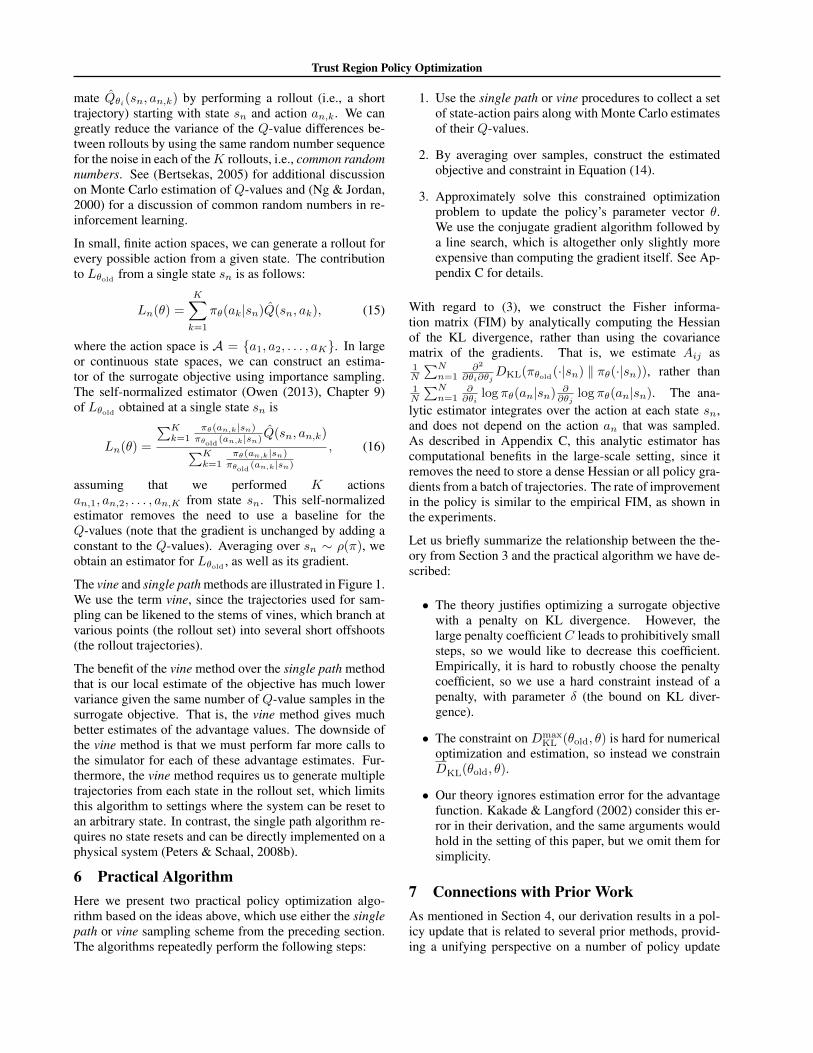
Figure 1. Left: illustration of single path procedure. Here, wegenerate a set of trajectories via simulation of the policy and in-corporate all state-action pairs (sn, an) into the objective. Right:illustration of vine procedure. We generate a set of “trunk” tra-jectories, and then generate “branch” rollouts from a subset of thereached states. For each of these states sn, we perform multipleactions (a1 and a2 here) and perform a rollout after each action,using common random numbers (CRN) to reduce the variance.

All that remains is to replace the expectations by sampleaverages and replace the Q value by an empirical estimate.The following sections describe two different schemes forperforming this estimation.

The first sampling scheme, which we call single path, isthe one that is typically used for policy gradient estima-tion (Bartlett & Baxter, 2011), and is based on samplingindividual trajectories. The second scheme, which we callvine, involves constructing a rollout set and then perform-ing multiple actions from each state in the rollout set. Thismethod has mostly been explored in the context of policy it-eration methods (Lagoudakis & Parr, 2003; Gabillon et al.,2013).

5.1 Single Path

In this estimation procedure, we collect a sequence ofstates by sampling s0 ∼ ρ0 and then simulating the pol-icy πθold for some number of timesteps to generate a trajec-tory s0, a0, s1, a1, . . . , sT−1, aT−1, sT . Hence, q(a|s) =πθold(a|s). Qθold(s, a) is computed at each state-actionpair (st, at) by taking the discounted sum of future rewardsalong the trajectory.

5.2 Vine

In this estimation procedure, we first sample s0 ∼ ρ0 andsimulate the policy πθi to generate a number of trajecto-ries. We then choose a subset of N states along these tra-jectories, denoted s1, s2, . . . , sN , which we call the “roll-out set”. For each state sn in the rollout set, we sampleK actions according to an,k ∼ q(·|sn). Any choice ofq(·|sn) with a support that includes the support of πθi(·|sn)will produce a consistent estimator. In practice, we foundthat q(·|sn) = πθi(·|sn) works well on continuous prob-lems, such as robotic locomotion, while the uniform dis-tribution works well on discrete tasks, such as the Atarigames, where it can sometimes achieve better exploration.

For each action an,k sampled at each state sn, we esti-


mate Qθi(sn, an,k) by performing a rollout (i.e., a shorttrajectory) starting with state sn and action an,k. We cangreatly reduce the variance of the Q-value differences be-tween rollouts by using the same random number sequencefor the noise in each of theK rollouts, i.e., common randomnumbers. See (Bertsekas, 2005) for additional discussionon Monte Carlo estimation of Q-values and (Ng & Jordan,2000) for a discussion of common random numbers in re-inforcement learning.

In small, finite action spaces, we can generate a rollout forevery possible action from a given state. The contributionto Lθold from a single state sn is as follows:

Ln(θ) =

K∑k=1

πθ(ak|sn)Q(sn, ak), (15)

where the action space is A = {a1, a2, . . . , aK}. In largeor continuous state spaces, we can construct an estima-tor of the surrogate objective using importance sampling.The self-normalized estimator (Owen (2013), Chapter 9)of Lθold obtained at a single state sn is

Ln(θ) =

∑Kk=1

πθ(an,k|sn)πθold (an,k|sn)

Q(sn, an,k)∑Kk=1

πθ(an,k|sn)πθold (an,k|sn)

, (16)

assuming that we performed K actionsan,1, an,2, . . . , an,K from state sn. This self-normalizedestimator removes the need to use a baseline for theQ-values (note that the gradient is unchanged by adding aconstant to the Q-values). Averaging over sn ∼ ρ(π), weobtain an estimator for Lθold , as well as its gradient.

The vine and single path methods are illustrated in Figure 1.We use the term vine, since the trajectories used for sam-pling can be likened to the stems of vines, which branch atvarious points (the rollout set) into several short offshoots(the rollout trajectories).

The benefit of the vine method over the single path methodthat is our local estimate of the objective has much lowervariance given the same number of Q-value samples in thesurrogate objective. That is, the vine method gives muchbetter estimates of the advantage values. The downside ofthe vine method is that we must perform far more calls tothe simulator for each of these advantage estimates. Fur-thermore, the vine method requires us to generate multipletrajectories from each state in the rollout set, which limitsthis algorithm to settings where the system can be reset toan arbitrary state. In contrast, the single path algorithm re-quires no state resets and can be directly implemented on aphysical system (Peters & Schaal, 2008b).

6 Practical AlgorithmHere we present two practical policy optimization algo-rithm based on the ideas above, which use either the singlepath or vine sampling scheme from the preceding section.The algorithms repeatedly perform the following steps:

1. Use the single path or vine procedures to collect a setof state-action pairs along with Monte Carlo estimatesof their Q-values.

2. By averaging over samples, construct the estimatedobjective and constraint in Equation (14).

3. Approximately solve this constrained optimizationproblem to update the policy’s parameter vector θ.We use the conjugate gradient algorithm followed bya line search, which is altogether only slightly moreexpensive than computing the gradient itself. See Ap-pendix C for details.

With regard to (3), we construct the Fisher informa-tion matrix (FIM) by analytically computing the Hessianof the KL divergence, rather than using the covariancematrix of the gradients. That is, we estimate Aij as1N

∑Nn=1

∂2

∂θi∂θjDKL(πθold(·|sn) ‖ πθ(·|sn)), rather than

1N

∑Nn=1

∂∂θi

log πθ(an|sn) ∂∂θj

log πθ(an|sn). The ana-lytic estimator integrates over the action at each state sn,and does not depend on the action an that was sampled.As described in Appendix C, this analytic estimator hascomputational benefits in the large-scale setting, since itremoves the need to store a dense Hessian or all policy gra-dients from a batch of trajectories. The rate of improvementin the policy is similar to the empirical FIM, as shown inthe experiments.

Let us briefly summarize the relationship between the the-ory from Section 3 and the practical algorithm we have de-scribed:

• The theory justifies optimizing a surrogate objectivewith a penalty on KL divergence. However, thelarge penalty coefficientC leads to prohibitively smallsteps, so we would like to decrease this coefficient.Empirically, it is hard to robustly choose the penaltycoefficient, so we use a hard constraint instead of apenalty, with parameter δ (the bound on KL diver-gence).

• The constraint on DmaxKL (θold, θ) is hard for numerical

optimization and estimation, so instead we constrainDKL(θold, θ).

• Our theory ignores estimation error for the advantagefunction. Kakade & Langford (2002) consider this er-ror in their derivation, and the same arguments wouldhold in the setting of this paper, but we omit them forsimplicity.

7 Connections with Prior WorkAs mentioned in Section 4, our derivation results in a pol-icy update that is related to several prior methods, provid-ing a unifying perspective on a number of policy update


schemes. The natural policy gradient (Kakade, 2002) canbe obtained as a special case of the update in Equation (12)by using a linear approximation to L and a quadratic ap-proximation to the DKL constraint, resulting in the follow-ing problem:

maximizeθ

[∇θLθold(θ)

∣∣θ=θold

· (θ − θold)]

(17)

subject to1

2(θold − θ)TA(θold)(θold − θ) ≤ δ,

where A(θold)ij =

∂

∂θi

∂

∂θjEs∼ρπ [DKL(π(·|s, θold) ‖ π(·|s, θ))]

∣∣θ=θold

.

The update is θnew = θold + 1λA(θold)−1∇θL(θ)

∣∣θ=θold

,where the stepsize 1

λ is typically treated as an algorithmparameter. This differs from our approach, which en-forces the constraint at each update. Though this differencemight seem subtle, our experiments demonstrate that it sig-nificantly improves the algorithm’s performance on largerproblems.

We can also obtain the standard policy gradient update byusing an `2 constraint or penalty:

maximizeθ

[∇θLθold(θ)

∣∣θ=θold

· (θ − θold)]

(18)

subject to1

2‖θ − θold‖2 ≤ δ.

The policy iteration update can also be obtained by solvingthe unconstrained problem maximizeπ Lπold

(π), using Las defined in Equation (3).

Several other methods employ an update similar to Equa-tion (12). Relative entropy policy search (REPS) (Peterset al., 2010) constrains the state-action marginals p(s, a),while TRPO constrains the conditionals p(a|s). UnlikeREPS, our approach does not require a costly nonlinear op-timization in the inner loop. Levine and Abbeel (2014) alsouse a KL divergence constraint, but its purpose is to encour-age the policy not to stray from regions where the estimateddynamics model is valid, while we do not attempt to esti-mate the system dynamics explicitly. Pirotta et al. (2013)also build on and generalize Kakade and Langford’s results,and they derive different algorithms from the ones here.

8 ExperimentsWe designed our experiments to investigate the followingquestions:

1. What are the performance characteristics of the singlepath and vine sampling procedures?

2. TRPO is related to prior methods (e.g. natural policygradient) but makes several changes, most notably byusing a fixed KL divergence rather than a fixed penaltycoefficient. How does this affect the performance ofthe algorithm?

Figure 2. 2D robot models used for locomotion experiments.From left to right: swimmer, hopper, walker. The hopper andwalker present a particular challenge, due to underactuation andcontact discontinuities.

Join

tang

les

and

kine

mat

ics

Control

Standarddeviations

Fullyconnected

layer

30 units

Inputlayer

Meanparameters Sampling

Scre

enin

put

4×4

4×4

4×4

4×4

4×4

4×4

4×4

4×4

Control

Hiddenlayer

20 units

Conv.layer

Conv.layer

Inputlayer

16 filters16 filters

Actionprobabilities Sampling

Figure 3. Neural networks used for the locomotion task (top) andfor playing Atari games (bottom).

3. Can TRPO be used to solve challenging large-scaleproblems? How does TRPO compare with othermethods when applied to large-scale problems, withregard to final performance, computation time, andsample complexity?

To answer (1) and (2), we compare the performance ofthe single path and vine variants of TRPO, several ablatedvariants, and a number of prior policy optimization algo-rithms. With regard to (3), we show that both the singlepath and vine algorithm can obtain high-quality locomo-tion controllers from scratch, which is considered to be ahard problem. We also show that these algorithms producecompetitive results when learning policies for playing Atarigames from images using convolutional neural networkswith tens of thousands of parameters.

8.1 Simulated Robotic Locomotion

We conducted the robotic locomotion experiments usingthe MuJoCo simulator (Todorov et al., 2012). The threesimulated robots are shown in Figure 2. The states of therobots are their generalized positions and velocities, and thecontrols are joint torques. Underactuation, high dimension-ality, and non-smooth dynamics due to contacts make these


tasks very challenging. The following models are includedin our evaluation:

1. Swimmer. 10-dimensional state space, linear rewardfor forward progress and a quadratic penalty on jointeffort to produce the reward r(x, u) = vx−10−5‖u‖2.The swimmer can propel itself forward by making anundulating motion.

2. Hopper. 12-dimensional state space, same reward asthe swimmer, with a bonus of +1 for being in a non-terminal state. We ended the episodes when the hop-per fell over, which was defined by thresholds on thetorso height and angle.

3. Walker. 18-dimensional state space. For the walker,we added a penalty for strong impacts of the feetagainst the ground to encourage a smooth walk ratherthan a hopping gait.

We used δ = 0.01 for all experiments. See Table 2 in theAppendix for more details on the experimental setup andparameters used. We used neural networks to represent thepolicy, with the architecture shown in Figure 3, and furtherdetails provided in Appendix D. To establish a standardbaseline, we also included the classic cart-pole balancingproblem, based on the formulation from Barto et al. (1983),using a linear policy with six parameters that is easy to opti-mize with derivative-free black-box optimization methods.

The following algorithms were considered in the compari-son: single path TRPO; vine TRPO; cross-entropy method(CEM), a gradient-free method (Szita & Lorincz, 2006);covariance matrix adaption (CMA), another gradient-freemethod (Hansen & Ostermeier, 1996); natural gradi-ent, the classic natural policy gradient algorithm (Kakade,2002), which differs from single path by the use of a fixedpenalty coefficient (Lagrange multiplier) instead of the KLdivergence constraint; empirical FIM, identical to singlepath, except that the FIM is estimated using the covariancematrix of the gradients rather than the analytic estimate;max KL, which was only tractable on the cart-pole problem,and uses the maximum KL divergence in Equation (11),rather than the average divergence, allowing us to evaluatethe quality of this approximation. The parameters used inthe experiments are provided in Appendix E. For the natu-ral gradient method, we swept through the possible valuesof the stepsize in factors of three, and took the best valueaccording to the final performance.

Learning curves showing the total reward averaged acrossfive runs of each algorithm are shown in Figure 4. Singlepath and vine TRPO solved all of the problems, yieldingthe best solutions. Natural gradient performed well on thetwo easier problems, but was unable to generate hoppingand walking gaits that made forward progress. These re-sults provide empirical evidence that constraining the KLdivergence is a more robust way to choose step sizes andmake fast, consistent progress, compared to using a fixed

0 10 20 30 40 50

number of policy iterations

0

2

4

6

8

10

reward

Cartpole

VineSingle PathNatural GradientMax KLEmpirical FIMCEMCMARWR

0 10 20 30 40 50


0.10

0.05

0.00

0.05

0.10

0.15

cost (-velocity + ctrl)

Swimmer

VineSingle PathNatural GradientEmpirical FIMCEMCMARWR

0 50 100 150 200


1.0

0.5

0.0

0.5

1.0

1.5

2.0

2.5

reward

Hopper

VineSingle PathNatural GradientCEMRWR

0 50 100 150 200


1.0

0.5

0.0

0.5

1.0

1.5

2.0

2.5

3.0

3.5

reward

WalkerVineSingle PathNatural GradientCEMRWR

Figure 4. Learning curves for locomotion tasks, averaged acrossfive runs of each algorithm with random initializations. Note thatfor the hopper and walker, a score of −1 is achievable without anyforward velocity, indicating a policy that simply learned balancedstanding, but not walking.

penalty. CEM and CMA are derivative-free algorithms,hence their sample complexity scales unfavorably with thenumber of parameters, and they performed poorly on thelarger problems. The max KL method learned somewhatmore slowly than our final method, due to the more restric-tive form of the constraint, but overall the result suggeststhat the average KL divergence constraint has a similar ef-fect as the theorecally justified maximum KL divergence.Videos of the policies learned by TRPO may be viewed onthe project website: http://sites.google.com/site/trpopaper/.

Note that TRPO learned all of the gaits with general-purpose policies and simple reward functions, using min-imal prior knowledge. This is in contrast with most priormethods for learning locomotion, which typically rely onhand-architected policy classes that explicitly encode no-tions of balance and stepping (Tedrake et al., 2004; Genget al., 2006; Wampler & Popovic, 2009).

8.2 Playing Games from Images

To evaluate TRPO on a partially observed task with com-plex observations, we trained policies for playing Atarigames, using raw images as input. The games requirelearning a variety of behaviors, such as dodging bullets andhitting balls with paddles. Aside from the high dimension-ality, challenging elements of these games include delayedrewards (no immediate penalty is incurred when a life islost in Breakout or Space Invaders); complex sequences ofbehavior (Q*bert requires a character to hop on 21 differ-ent platforms); and non-stationary image statistics (Enduroinvolves a changing and flickering background).

We tested our algorithms on the same seven games reportedon in (Mnih et al., 2013) and (Guo et al., 2014), which are

http://sites.google.com/site/trpopaper/

http://sites.google.com/site/trpopaper/


B. Rider Breakout Enduro Pong Q*bert Seaquest S. Invaders

Random 354 1.2 0 −20.4 157 110 179Human (Mnih et al., 2013) 7456 31.0 368 −3.0 18900 28010 3690

Deep Q Learning (Mnih et al., 2013) 4092 168.0 470 20.0 1952 1705 581

UCC-I (Guo et al., 2014) 5702 380 741 21 20025 2995 692

TRPO - single path 1425.2 10.8 534.6 20.9 1973.5 1908.6 568.4TRPO - vine 859.5 34.2 430.8 20.9 7732.5 788.4 450.2

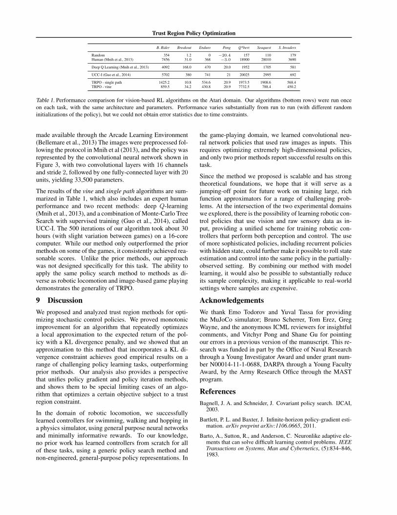
Table 1. Performance comparison for vision-based RL algorithms on the Atari domain. Our algorithms (bottom rows) were run onceon each task, with the same architecture and parameters. Performance varies substantially from run to run (with different randominitializations of the policy), but we could not obtain error statistics due to time constraints.

made available through the Arcade Learning Environment(Bellemare et al., 2013) The images were preprocessed fol-lowing the protocol in Mnih et al (2013), and the policy wasrepresented by the convolutional neural network shown inFigure 3, with two convolutional layers with 16 channelsand stride 2, followed by one fully-connected layer with 20units, yielding 33,500 parameters.

The results of the vine and single path algorithms are sum-marized in Table 1, which also includes an expert humanperformance and two recent methods: deep Q-learning(Mnih et al., 2013), and a combination of Monte-Carlo TreeSearch with supervised training (Guo et al., 2014), calledUCC-I. The 500 iterations of our algorithm took about 30hours (with slight variation between games) on a 16-corecomputer. While our method only outperformed the priormethods on some of the games, it consistently achieved rea-sonable scores. Unlike the prior methods, our approachwas not designed specifically for this task. The ability toapply the same policy search method to methods as di-verse as robotic locomotion and image-based game playingdemonstrates the generality of TRPO.

9 DiscussionWe proposed and analyzed trust region methods for opti-mizing stochastic control policies. We proved monotonicimprovement for an algorithm that repeatedly optimizesa local approximation to the expected return of the pol-icy with a KL divergence penalty, and we showed that anapproximation to this method that incorporates a KL di-vergence constraint achieves good empirical results on arange of challenging policy learning tasks, outperformingprior methods. Our analysis also provides a perspectivethat unifies policy gradient and policy iteration methods,and shows them to be special limiting cases of an algo-rithm that optimizes a certain objective subject to a trustregion constraint.

In the domain of robotic locomotion, we successfullylearned controllers for swimming, walking and hopping ina physics simulator, using general purpose neural networksand minimally informative rewards. To our knowledge,no prior work has learned controllers from scratch for allof these tasks, using a generic policy search method andnon-engineered, general-purpose policy representations. In

the game-playing domain, we learned convolutional neu-ral network policies that used raw images as inputs. Thisrequires optimizing extremely high-dimensional policies,and only two prior methods report successful results on thistask.

Since the method we proposed is scalable and has strongtheoretical foundations, we hope that it will serve as ajumping-off point for future work on training large, richfunction approximators for a range of challenging prob-lems. At the intersection of the two experimental domainswe explored, there is the possibility of learning robotic con-trol policies that use vision and raw sensory data as in-put, providing a unified scheme for training robotic con-trollers that perform both perception and control. The useof more sophisticated policies, including recurrent policieswith hidden state, could further make it possible to roll stateestimation and control into the same policy in the partially-observed setting. By combining our method with modellearning, it would also be possible to substantially reduceits sample complexity, making it applicable to real-worldsettings where samples are expensive.

AcknowledgementsWe thank Emo Todorov and Yuval Tassa for providingthe MuJoCo simulator; Bruno Scherrer, Tom Erez, GregWayne, and the anonymous ICML reviewers for insightfulcomments, and Vitchyr Pong and Shane Gu for pointingour errors in a previous version of the manuscript. This re-search was funded in part by the Office of Naval Researchthrough a Young Investigator Award and under grant num-ber N00014-11-1-0688, DARPA through a Young FacultyAward, by the Army Research Office through the MASTprogram.

ReferencesBagnell, J. A. and Schneider, J. Covariant policy search. IJCAI,

2003.

Bartlett, P. L. and Baxter, J. Infinite-horizon policy-gradient esti-mation. arXiv preprint arXiv:1106.0665, 2011.

Barto, A., Sutton, R., and Anderson, C. Neuronlike adaptive ele-ments that can solve difficult learning control problems. IEEETransactions on Systems, Man and Cybernetics, (5):834–846,1983.


Bellemare, M. G., Naddaf, Y., Veness, J., and Bowling, M. The ar-cade learning environment: An evaluation platform for generalagents. Journal of Artificial Intelligence Research, 47:253–279, jun 2013.

Bertsekas, D. Dynamic programming and optimal control, vol-ume 1. 2005.

Deisenroth, M., Neumann, G., and Peters, J. A survey on policysearch for robotics. Foundations and Trends in Robotics, 2(1-2):1–142, 2013.

Gabillon, Victor, Ghavamzadeh, Mohammad, and Scherrer,Bruno. Approximate dynamic programming finally performswell in the game of Tetris. In Advances in Neural InformationProcessing Systems, 2013.

Geng, T., Porr, B., and Worgotter, F. Fast biped walking with areflexive controller and realtime policy searching. In Advancesin Neural Information Processing Systems (NIPS), 2006.

Guo, X., Singh, S., Lee, H., Lewis, R. L., and Wang, X. Deeplearning for real-time atari game play using offline Monte-Carlo tree search planning. In Advances in Neural InformationProcessing Systems, pp. 3338–3346, 2014.

Hansen, Nikolaus and Ostermeier, Andreas. Adapting arbitrarynormal mutation distributions in evolution strategies: The co-variance matrix adaptation. In Evolutionary Computation,1996., Proceedings of IEEE International Conference on, pp.312–317. IEEE, 1996.

Hunter, David R and Lange, Kenneth. A tutorial on MM algo-rithms. The American Statistician, 58(1):30–37, 2004.

Kakade, Sham. A natural policy gradient. In Advances in NeuralInformation Processing Systems, pp. 1057–1063. MIT Press,2002.

Kakade, Sham and Langford, John. Approximately optimal ap-proximate reinforcement learning. In ICML, volume 2, pp.267–274, 2002.

Lagoudakis, Michail G and Parr, Ronald. Reinforcement learn-ing as classification: Leveraging modern classifiers. In ICML,volume 3, pp. 424–431, 2003.

Levin, D. A., Peres, Y., and Wilmer, E. L. Markov chains andmixing times. American Mathematical Society, 2009.

Levine, Sergey and Abbeel, Pieter. Learning neural networkpolicies with guided policy search under unknown dynamics.In Advances in Neural Information Processing Systems, pp.1071–1079, 2014.

Martens, J. and Sutskever, I. Training deep and recurrent networkswith hessian-free optimization. In Neural Networks: Tricks ofthe Trade, pp. 479–535. Springer, 2012.

Mnih, V., Kavukcuoglu, K., Silver, D., Graves, A., Antonoglou,I., Wierstra, D., and Riedmiller, M. Playing Atari with deepreinforcement learning. arXiv preprint arXiv:1312.5602, 2013.

Nemirovski, Arkadi. Efficient methods in convex programming.2005.

Ng, A. Y. and Jordan, M. PEGASUS: A policy search methodfor large mdps and pomdps. In Uncertainty in artificial intelli-gence (UAI), 2000.

Owen, Art B. Monte Carlo theory, methods and examples. 2013.

Pascanu, Razvan and Bengio, Yoshua. Revisiting natural gradientfor deep networks. arXiv preprint arXiv:1301.3584, 2013.

Peters, J. and Schaal, S. Reinforcement learning of motorskills with policy gradients. Neural Networks, 21(4):682–697,2008a.

Peters, J., Mulling, K., and Altun, Y. Relative entropy policysearch. In AAAI Conference on Artificial Intelligence, 2010.

Peters, Jan and Schaal, Stefan. Natural actor-critic. Neurocom-puting, 71(7):1180–1190, 2008b.

Pirotta, Matteo, Restelli, Marcello, Pecorino, Alessio, and Calan-driello, Daniele. Safe policy iteration. In Proceedings of The30th International Conference on Machine Learning, pp. 307–315, 2013.

Pollard, David. Asymptopia: an exposition of statistical asymp-totic theory. 2000. URL http://www.stat.yale.edu/˜pollard/Books/Asymptopia.

Szita, Istvan and Lorincz, Andras. Learning tetris using thenoisy cross-entropy method. Neural computation, 18(12):2936–2941, 2006.

Tedrake, R., Zhang, T., and Seung, H. Stochastic policy gradi-ent reinforcement learning on a simple 3d biped. In IEEE/RSJInternational Conference on Intelligent Robots and Systems,2004.

Todorov, Emanuel, Erez, Tom, and Tassa, Yuval. MuJoCo: Aphysics engine for model-based control. In Intelligent Robotsand Systems (IROS), 2012 IEEE/RSJ International Conferenceon, pp. 5026–5033. IEEE, 2012.

Wampler, Kevin and Popovic, Zoran. Optimal gait and form foranimal locomotion. In ACM Transactions on Graphics (TOG),volume 28, pp. 60. ACM, 2009.

Wright, Stephen J and Nocedal, Jorge. Numerical optimization,volume 2. Springer New York, 1999.

http://www.stat.yale.edu/~pollard/Books/Asymptopia

http://www.stat.yale.edu/~pollard/Books/Asymptopia


A Proof of Policy Improvement BoundThis proof (of Theorem 1) uses techniques from the proof of Theorem 4.1 in (Kakade & Langford, 2002), adapting themto the more general setting considered in this paper. An informal overview is as follows. Our proof relies on the notionof coupling, where we jointly define the policies π and π′ so that they choose the same action with high probability= (1 − α). Surrogate loss Lπ(π) accounts for the the advantage of π the first time that it disagrees with π, but notsubsequent disagreements. Hence, the error in Lπ is due to two or more disagreements between π and π, hence, we get anO(α2) correction term, where α is the probability of disagreement.

We start out with a lemma from Kakade & Langford (2002) that shows that the difference in policy performance η(π)−η(π)can be decomposed as a sum of per-timestep advantages.Lemma 1. Given two policies π, π,

η(π) = η(π)+Eτ∼π

[ ∞∑t=0

γtAπ(st, at)

](19)

This expectation is taken over trajectories τ := (s0, a0, s1, a0, . . . ), and the notation Eτ∼π [. . . ] indicates that actions aresampled from π to generate τ .

Proof. First note that Aπ(s, a) = Es′∼P (s′|s,a) [r(s) + γVπ(s′)− Vπ(s)]. Therefore,

Eτ |π

[ ∞∑t=0

γtAπ(st, at)

](20)

= Eτ |π

[ ∞∑t=0

γt(r(st) + γVπ(st+1)− Vπ(st))

](21)

= Eτ |π

[−Vπ(s0) +

∞∑t=0

γtr(st)

](22)

= −Es0 [Vπ(s0)] + Eτ |π

[ ∞∑t=0

γtr(st)

](23)

= −η(π) + η(π) (24)

Rearranging, the result follows.

Define A(s) to be the expected advantage of π over π at state s:

A(s) = Ea∼π(·|s) [Aπ(s, a)] . (25)

Now Lemma 1 can be written as follows:

η(π) = η(π) + Eτ∼π

[ ∞∑t=0

γtA(st)

](26)

Note that Lπ can be written as

Lπ(π) = η(π) + Eτ∼π

[ ∞∑t=0

γtA(st)

](27)

The difference in these equations is whether the states are sampled using π or π. To bound the difference between η(π) andLπ(π), we will bound the difference arising from each timestep. To do this, we first need to introduce a measure of howmuch π and π agree. Specifically, we’ll couple the policies, so that they define a joint distribution over pairs of actions.Definition 1. (π, π) is an α-coupled policy pair if it defines a joint distribution (a, a)|s, such that P (a 6= a|s) ≤ α for alls. π and π will denote the marginal distributions of a and a, respectively.


Computationally, α-coupling means that if we randomly choose a seed for our random number generator, and then wesample from each of π and π after setting that seed, the results will agree for at least fraction 1− α of seeds.

Lemma 2. Given that π, π are α-coupled policies, for all s,∣∣A(s)∣∣ ≤ 2αmax

s,a|Aπ(s, a)| (28)

Proof.

A(s) = Ea∼π [Aπ(s, a)] = E(a,a)∼(π,π) [Aπ(s, a)−Aπ(s, a)] since Ea∼π [Aπ(s, a)] = 0 (29)

= P (a 6= a|s)E(a,a)∼(π,π)|a6=a [Aπ(s, a)−Aπ(s, a)] (30)

|A(s)| ≤ α · 2 maxs,a|Aπ(s, a)| (31)

Lemma 3. Let (π, π) be an α-coupled policy pair. Then∣∣Est∼π [A(st)]− Est∼π

[A(st)

]∣∣ ≤ 2αmaxsA(s) ≤ 4α(1− (1− α)t) max

s|Aπ(s, a)| (32)

Proof. Given the coupled policy pair (π, π), we can also obtain a coupling over the trajectory distributions produced byπ and π, respectively. Namely, we have pairs of trajectories τ, τ , where τ is obtained by taking actions from π, and τ isobtained by taking actions from π, where the same random seed is used to generate both trajectories. We will considerthe advantage of π over π at timestep t, and decompose this expectation based on whether π agrees with π at all timestepsi < t.

Let nt denote the number of times that ai 6= ai for i < t, i.e., the number of times that π and π disagree before timestep t.

Est∼π[A(st)

]= P (nt = 0)Est∼π|nt=0

[A(st)

]+ P (nt > 0)Est∼π|nt>0

[A(st)

](33)

The expectation decomposes similarly for actions are sampled using π:

Est∼π[A(st)

]= P (nt = 0)Est∼π|nt=0

[A(st)

]+ P (nt > 0)Est∼π|nt>0

[A(st)

](34)

Note that the nt = 0 terms are equal:

Est∼π|nt=0

[A(st)

]= Est∼π|nt=0

[A(st)

], (35)

because nt = 0 indicates that π and π agreed on all timesteps less than t. Subtracting Equations (33) and (34), we get

Est∼π[A(st)

]− Est∼π

[A(st)

]= P (nt > 0)

(Est∼π|nt>0

[A(st)

]− Est∼π|nt>0

[A(st)

])(36)

By definition of α, P (π, π agree at timestep i) ≥ 1− α, so P (nt = 0) ≥ (1− α)t, and

P (nt > 0) ≤ 1− (1− α)t (37)

Next, note that∣∣Est∼π|nt>0

[A(st)

]− Est∼π|nt>0

[A(st)

]∣∣ ≤ ∣∣Est∼π|nt>0

[A(st)

]∣∣+∣∣Est∼π|nt>0

[A(st)

]∣∣ (38)

≤ 4αmaxs,a|Aπ(s, a)| (39)

Where the second inequality follows from Lemma 3.

Plugging Equation (37) and Equation (39) into Equation (36), we get∣∣Est∼π [A(st)]− Est∼π

[A(st)

]∣∣ ≤ 4α(1− (1− α)t) maxs,a|Aπ(s, a)| (40)


The preceding Lemma bounds the difference in expected advantage at each timestep t. We can sum over time to bound thedifference between η(π) and Lπ(π). Subtracting Equation (26) and Equation (27), and defining ε = maxs,a |Aπ(s, a)|,

|η(π)− Lπ(π)| =∞∑t=0

γt∣∣Eτ∼π [A(st)

]− Eτ∼π

[A(st)

]∣∣ (41)

≤∞∑t=0

γt · 4εα(1− (1− α)t) (42)

= 4εα

(1

1− γ− 1

1− γ(1− α)

)(43)

=4α2γε

(1− γ)(1− γ(1− α))(44)

≤ 4α2γε

(1− γ)2(45)

Last, to replace α by the total variation divergence, we need to use the correspondence between TV divergence and coupledrandom variables:

Suppose pX and pY are distributions with DTV (pX ‖ pY ) = α. Then there exists a joint distribution (X,Y )whose marginals are pX , pY , for which X = Y with probability 1− α.

See (Levin et al., 2009), Proposition 4.7.

It follows that if we have two policies π and π such that maxsDTV (π(·|s) ‖ π(·|s)) ≤ α, then we can define an α-coupledpolicy pair (π, π) with appropriate marginals. Taking α = maxsDTV (π(·|s) ‖ π(·|s)) ≤ α in Equation (45), Theorem 1follows.

B Perturbation Theory Proof of Policy Improvement BoundWe also provide an alternative proof of Theorem 1 using perturbation theory.

Proof. LetG = (1+γPπ+(γPπ)2+. . . ) = (1−γPπ)−1, and similarly Let G = (1+γPπ+(γPπ)2+. . . ) = (1−γPπ)−1.We will use the convention that ρ (a density on state space) is a vector and r (a reward function on state space) is a dualvector (i.e., linear functional on vectors), thus rρ is a scalar meaning the expected reward under density ρ. Note thatη(π) = rGρ0, and η(π) = cGρ0. Let ∆ = Pπ − Pπ . We want to bound η(π)− η(π) = r(G−G)ρ0. We start with somestandard perturbation theory manipulations.

G−1 − G−1 = (1− γPπ)− (1− γPπ)

= γ∆. (46)

Left multiply by G and right multiply by G.

G−G = γG∆G

G = G+ γG∆G (47)

Substituting the right-hand side into G gives

G = G+ γG∆G+ γ2G∆G∆G (48)

So we have

η(π)− η(π) = r(G−G)ρ = γrG∆Gρ0 + γ2rG∆G∆Gρ0 (49)

Let us first consider the leading term γrG∆Gρ0. Note that rG = v, i.e., the infinite-horizon state-value function. Alsonote that Gρ0 = ρπ . Thus we can write γcG∆Gρ0 = γv∆ρπ . We will show that this expression equals the expected


advantage Lπ(π)− Lπ(π).

Lπ(π)− Lπ(π) =∑s

ρπ(s)∑a

(π(a|s)− π(a|s))Aπ(s, a)

=∑s

ρπ(s)∑a

(πθ(a|s)− πθ(a|s)

) [r(s) +

∑s′

p(s′|s, a)γv(s′)− v(s)

]=∑s

ρπ(s)∑s′

∑a

(π(a|s)− π(a|s)) p(s′|s, a)γv(s′)

=∑s

ρπ(s)∑s′

(pπ(s′|s)− pπ(s′|s))γv(s′)

= γv∆ρπ (50)

Next let us bound the O(∆2) term γ2rG∆G∆Gρ. First we consider the product γrG∆ = γv∆. Consider the components of this dual vector.

|(γv∆)s| =

∣∣∣∣∣∑a

(π(s, a)− π(s, a))Qπ(s, a)

∣∣∣∣∣=

∣∣∣∣∣∑a

(π(s, a)− π(s, a))Aπ(s, a)

∣∣∣∣∣≤∑a

|π(s, a)− π(s, a)| ·maxa|Aπ(s, a)|

≤ 2αε (51)

where the last line used the definition of the total-variation divergence, and the definition of ε = maxs,a |Aπ(s, a)|. Webound the other portion G∆Gρ using the `1 operator norm

‖A‖1 = supρ

{‖Aρ‖1‖ρ‖1

}(52)

where we have that ‖G‖1 = ‖G‖1 = 1/(1− γ) and ‖∆‖1 = 2α. That gives

‖G∆Gρ‖1 ≤ ‖G‖1‖∆‖1‖G‖1‖ρ‖1

=1

1− γ· 2α · 1

1− γ· 1 (53)

So we have that

γ2∣∣∣rG∆G∆Gρ

∣∣∣ ≤ γ‖γrG∆‖∞‖G∆Gρ‖1

≤ γ‖v∆‖∞‖G∆Gρ‖1

≤ γ · 2αε · 2α

(1− γ)2

=4γε

(1− γ)2α2 (54)

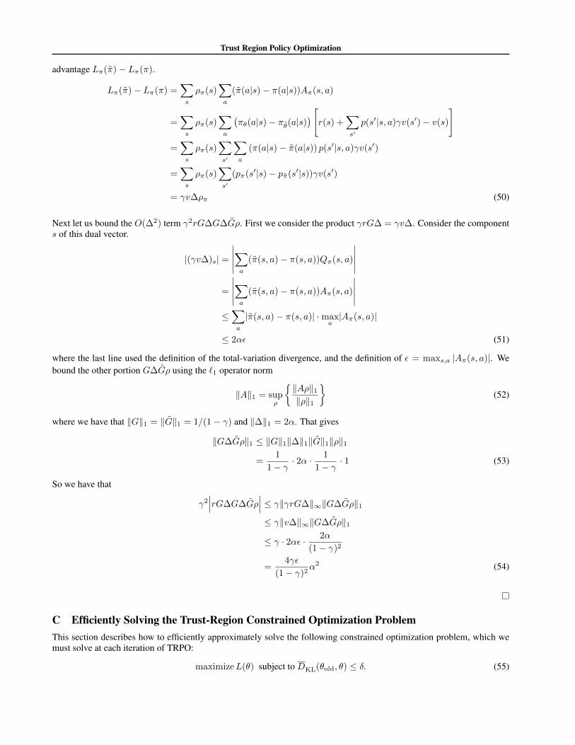
C Efficiently Solving the Trust-Region Constrained Optimization ProblemThis section describes how to efficiently approximately solve the following constrained optimization problem, which wemust solve at each iteration of TRPO:

maximizeL(θ) subject to DKL(θold, θ) ≤ δ. (55)


The method we will describe involves two steps: (1) compute a search direction, using a linear approximation to objectiveand quadratic approximation to the constraint; and (2) perform a line search in that direction, ensuring that we improve thenonlinear objective while satisfying the nonlinear constraint.

The search direction is computed by approximately solving the equation Ax = g, where A is the Fisher informationmatrix, i.e., the quadratic approximation to the KL divergence constraint: DKL(θold, θ) ≈ 1

2 (θ−θold)TA(θ−θold), whereAij = ∂

∂θi∂∂θj

DKL(θold, θ). In large-scale problems, it is prohibitively costly (with respect to computation and memory) toform the full matrix A (or A−1). However, the conjugate gradient algorithm allows us to approximately solve the equationAx = b without forming this full matrix, when we merely have access to a function that computes matrix-vector productsy → Ay. Appendix C.1 describes the most efficient way to compute matrix-vector products with the Fisher informationmatrix. For additional exposition on the use of Hessian-vector products for optimizing neural network objectives, see(Martens & Sutskever, 2012) and (Pascanu & Bengio, 2013).

Having computed the search direction s ≈ A−1g, we next need to compute the maximal step length β such that θ + βswill satisfy the KL divergence constraint. To do this, let δ = DKL ≈ 1

2 (βs)TA(βs) = 12β

2sTAs. From this, we obtainβ =

√2δ/sTAs, where δ is the desired KL divergence. The term sTAs can be computed through a single Hessian vector

product, and it is also an intermediate result produced by the conjugate gradient algorithm.

Last, we use a line search to ensure improvement of the surrogate objective and satisfaction of the KL divergence constraint,both of which are nonlinear in the parameter vector θ (and thus depart from the linear and quadratic approximations usedto compute the step). We perform the line search on the objective Lθold(θ) − X [DKL(θold, θ) ≤ δ], where X [. . . ] equalszero when its argument is true and +∞ when it is false. Starting with the maximal value of the step length β computedin the previous paragraph, we shrink β exponentially until the objective improves. Without this line search, the algorithmoccasionally computes large steps that cause a catastrophic degradation of performance.

C.1 Computing the Fisher-Vector Product

Here we will describe how to compute the matrix-vector product between the averaged Fisher information matrix andarbitrary vectors. This matrix-vector product enables us to perform the conjugate gradient algorithm. Suppose that theparameterized policy maps from the input x to “distribution parameter” vector µθ(x), which parameterizes the distributionπ(u|x). Now the KL divergence for a given input x can be written as follows:

DKL(πθold(·|x) ‖ πθ(·|x)) = kl(µθ(x), µold) (56)

where kl is the KL divergence between the distributions corresponding to the two mean parameter vectors. Differentiatingkl twice with respect to θ, we obtain

∂µa(x)

∂θi

∂µb(x)

∂θjkl′′ab(µθ(x), µold) +

∂2µa(x)

∂θi∂θjkl′a(µθ(x), µold) (57)

where the primes (′) indicate differentiation with respect to the first argument, and there is an implied summation overindices a, b. The second term vanishes, leaving just the first term. Let J := ∂µa(x)

∂θi(the Jacobian), then the Fisher

information matrix can be written in matrix form as JTMJ , where M = kl′′ab(µθ(x), µold) is the Fisher informationmatrix of the distribution in terms of the mean parameter µ (as opposed to the parameter θ). This has a simple form formost parameterized distributions of interest.

The Fisher-vector product can now be written as a function y → JTMJy. Multiplication by JT and J can be performed bymost automatic differentiation and neural network packages (multiplication by JT is the well-known backprop operation),and the operation for multiplication byM can be derived for the distribution of interest. Note that this Fisher-vector productis straightforward to average over a set of datapoints, i.e., inputs x to µ.

One could alternatively use a generic method for calculating Hessian-vector products using reverse mode automatic differ-entiation ((Wright & Nocedal, 1999), chapter 8), computing the Hessian of DKL with respect to θ. This method would beslightly less efficient as it does not exploit the fact that the second derivatives of µ(x) (i.e., the second term in Equation (57))can be ignored, but may be substantially easier to implement.

We have described a procedure for computing the Fisher-vector product y → Ay, where the Fisher information matrix isaveraged over a set of inputs to the function µ. Computing the Fisher-vector product is typically about as expensive ascomputing the gradient of an objective that depends on µ(x) (Wright & Nocedal, 1999). Furthermore, we need to compute


k of these Fisher-vector products per gradient, where k is the number of iterations of the conjugate gradient algorithm weperform. We found k = 10 to be quite effective, and using higher k did not result in faster policy improvement. Hence, anaıve implementation would spend more than 90% of the computational effort on these Fisher-vector products. However,we can greatly reduce this burden by subsampling the data for the computation of Fisher-vector product. Since the Fisherinformation matrix merely acts as a metric, it can be computed on a subset of the data without severely degrading thequality of the final step. Hence, we can compute it on 10% of the data, and the total cost of Hessian-vector products willbe about the same as computing the gradient. With this optimization, the computation of a natural gradient step A−1g doesnot incur a significant extra computational cost beyond computing the gradient g.

D Approximating Factored Policies with Neural NetworksThe policy, which is a conditional probability distribution πθ(a|s), can be parameterized with a neural network. Thisneural network maps (deterministically) from the state vector s to a vector µ, which specifies a distribution over actionspace. Then we can compute the likelihood p(a|µ) and sample a ∼ p(a|µ).

For our experiments with continuous state and action spaces, we used a Gaussian distribution, where the covariance matrixwas diagonal and independent of the state. A neural network with several fully-connected (dense) layers maps from theinput features to the mean of a Gaussian distribution. A separate set of parameters specifies the log standard deviation ofeach element. More concretely, the parameters include a set of weights and biases for the neural network computing themean, {Wi, bi}Li=1, and a vector r (log standard deviation) with the same dimension as a. Then, the policy is defined by

the normal distribution N(

mean = NeuralNet(s; {Wi, bi}Li=1

), stdev = exp(r)

). Here, µ = [mean, stdev].

For the experiments with discrete actions (Atari), we use a factored discrete action space, where each factor is parameter-ized as a categorical distribution. That is, the action consists of a tuple (a1, a2, . . . , aK) of integers ak ∈ {1, 2, . . . , Nk},and each of these components is assumed to have a categorical distribution, which is specified by a vector µk =[p1, p2, . . . , pNk ]. Hence, µ is defined to be the concatenation of the factors’ parameters: µ = [µ1, µ2, . . . , µK ] andhas dimension dimµ =

∑Kk=1Nk. The components of µ are computed by taking applying a neural network to the input s

and then applying the softmax operator to each slice, yielding normalized probabilities for each factor.

E Experiment Parameters

Swimmer Hopper WalkerState space dim. 10 12 20Control space dim. 2 3 6Total num. policy params 364 4806 8206Sim. steps per iter. 50K 1M 1MPolicy iter. 200 200 200Stepsize (DKL) 0.01 0.01 0.01Hidden layer size 30 50 50Discount (γ) 0.99 0.99 0.99Vine: rollout length 50 100 100Vine: rollouts per state 4 4 4Vine: Q-values per batch 500 2500 2500Vine: num. rollouts for sampling 16 16 16Vine: len. rollouts for sampling 1000 1000 1000Vine: computation time (minutes) 2 14 40SP: num. path 50 1000 10000SP: path len. 1000 1000 1000SP: computation time 5 35 100

Table 2. Parameters for continuous control tasks, vine and single path (SP) algorithms.


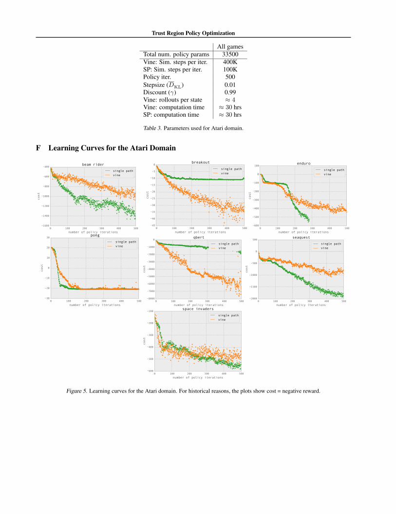
All gamesTotal num. policy params 33500Vine: Sim. steps per iter. 400KSP: Sim. steps per iter. 100KPolicy iter. 500Stepsize (DKL) 0.01Discount (γ) 0.99Vine: rollouts per state ≈ 4Vine: computation time ≈ 30 hrsSP: computation time ≈ 30 hrs

Table 3. Parameters used for Atari domain.

F Learning Curves for the Atari Domain

0 100 200 300 400 500


1600

1400

1200

1000

800

600

400

cost

beam rider

single pathvine

0 100 200 300 400 500


45

40

35

30

25

20

15

10

5

0

cost

breakout

single pathvine

0 100 200 300 400 500


600

500

400

300

200

100

0

100

cost

enduro

single pathvine

0 100 200 300 400 500


30

20

10

0

10

20

30

cost

pong

single pathvine

0 100 200 300 400 500


8000

7000

6000

5000

4000

3000

2000

1000

0

cost

qbert

single pathvine

0 100 200 300 400 500


2000

1500

1000

500

0

500

cost

seaquest

single pathvine

0 100 200 300 400 500


600

500

400

300

200

100

cost

space invaders

single pathvine

Figure 5. Learning curves for the Atari domain. For historical reasons, the plots show cost = negative reward.

Trust Region Policy Optimization - arXiv · parameterizations (Wampler & Popovi´c, 2009). The...

Documents

Transcript of Trust Region Policy Optimization - arXiv · parameterizations (Wampler & Popovi´c, 2009). The...