Truncated Regression and Sample Selection

RS – EC 2: Lecture 9

1

Lecture 9

Models for Censored and

Truncated Data – Truncated

Regression and Sample Selection

Censored and Truncated Data: Definitions

• Y is censored when we observe X for all observations, but we only know the true value of Y for a restricted range of observations. Values of Y in a certain range are reported as a single value or there is significant clustering around a value, say 0.

- If Y = k or Y > k for all Y => Y is censored from below or left-censored.

- If Y = k or Y < k for all Y => Y is censored from above or right-censored.

We usually think of an uncensored Y, Y*, the true value of Y when the censoring mechanism is not applied. We typically have all the observations for {Y,X}, but not {Y*,X}.

• Y is truncated when we only observe X for observations where Ywould not be censored. We do not have a full sample for {Y,X}, we exclude observations based on characteristics of Y.


Censored from below

0

2

4

6

8

10

0 2 4 6

x

y

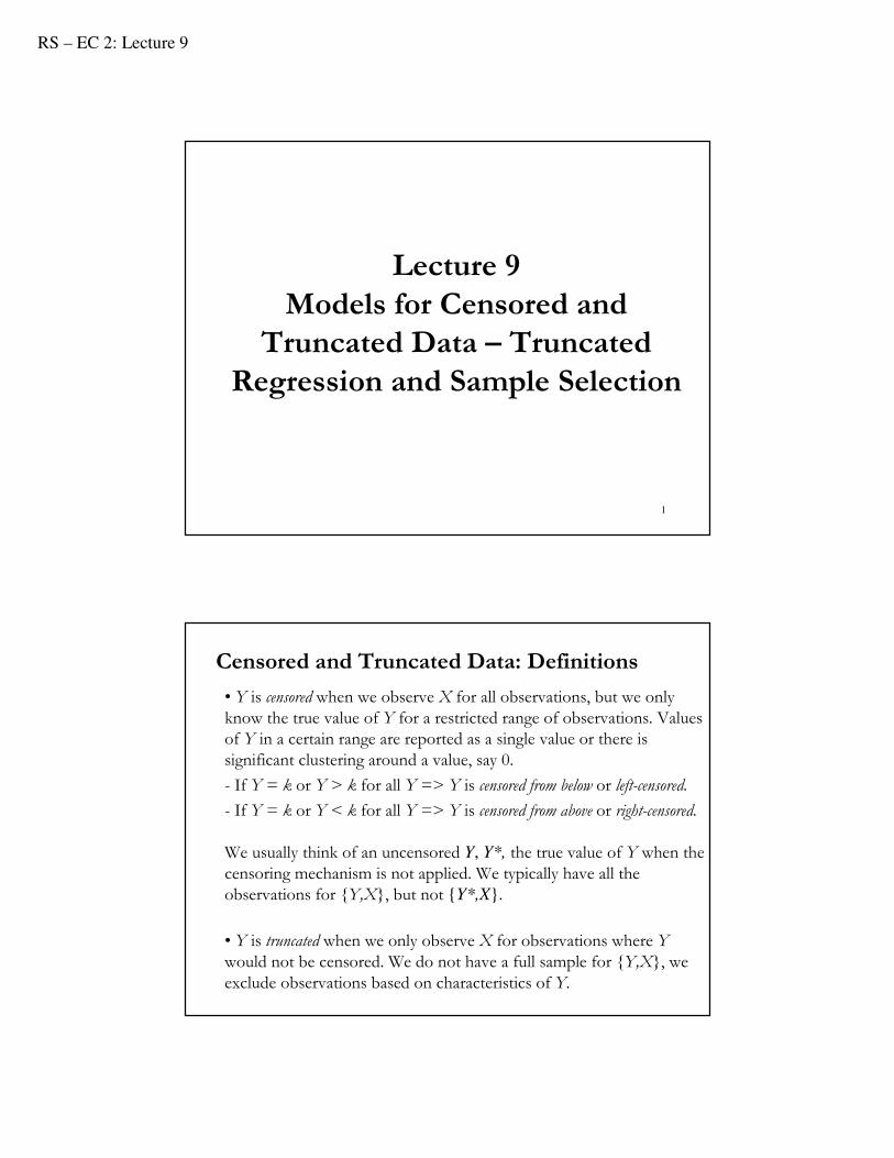
Censored from below: Example

• If Y ≤ 5, we do not know its exact value.

Example: A Central Bank intervenes if the exchange rate hits the band’s lower limit. => If St ≤ Ē => St= Ē.

4

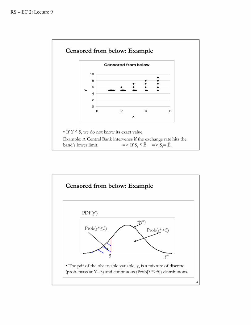
f(y*)

Prob(y*>5)

y*5

Prob(y*<5)

PDF(y*)

• The pdf of the observable variable, y, is a mixture of discrete (prob. mass at Y=5) and continuous (Prob[Y*>5]) distributions.



5

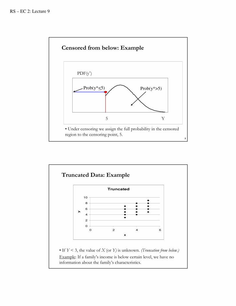
Prob(y*<5)

Y

Prob(y*>5)

5

PDF(y*)

• Under censoring we assign the full probability in the censored region to the censoring point, 5.


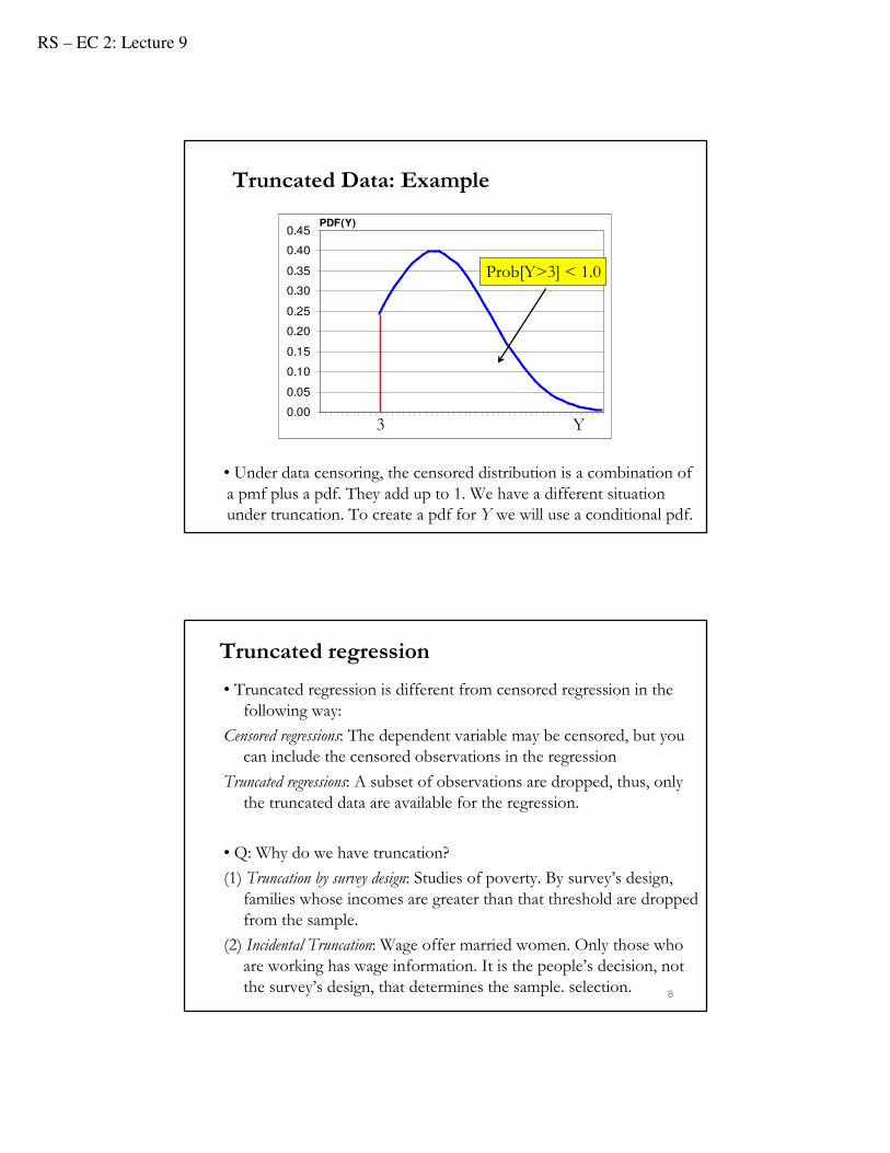
• If Y < 3, the value of X (or Y) is unknown. (Truncation from below.)

Example: If a family’s income is below certain level, we have no information about the family’s characteristics.

Truncated

0

2

4

6

8

10

0 2 4 6

x

y

Truncated Data: Example


• Under data censoring, the censored distribution is a combination of a pmf plus a pdf. They add up to 1. We have a different situation under truncation. To create a pdf for Y we will use a conditional pdf.

0.00

0.05

0.10

0.15

0.20

0.25

0.30

0.35

0.40

0.45

1 5 9 13 17 21 25 29 33 37 41 45 49

PDF(Y)

Prob[Y>3] < 1.0

3 Y

Truncated Data: Example

Truncated regression

• Truncated regression is different from censored regression in the following way:

Censored regressions: The dependent variable may be censored, but you can include the censored observations in the regression

Truncated regressions: A subset of observations are dropped, thus, only the truncated data are available for the regression.

• Q: Why do we have truncation?

(1) Truncation by survey design: Studies of poverty. By survey’s design, families whose incomes are greater than that threshold are dropped from the sample.

(2) Incidental Truncation: Wage offer married women. Only those who are working has wage information. It is the people’s decision, not the survey’s design, that determines the sample. selection.

8


Truncation and OLS

Q: What happens when we apply OLS to a truncated data?

- Suppose that you consider the following regression:

yi= β0 + β1xi + εi,

- We have a random sample of size N. All CLM assumptions are satisfied. (The most important assumption is (A2) E(εi|xi)=0.)

- Instead of using all the N observations, we use a subsample. Then, run OLS using this sub-sample (truncated sample) only.

• Q: Under what conditions, does sample selection matter to OLS?

(A) OLS is Unbiased

(A-1) Sample selection is randomly done.

(A-2) Sample selection is determined solely by the value of x-variable. For example, suppose that x is age. Then if you select sample if age is greater than 20 years old, this OLS is unbiased. 9

(B) OLS is Biased

(B-1) Sample selection is determined by the value of y-variable.

Example: Y is family income. We select the sample if y is greater than certain threshold. Then this OLS is biased.

(B-2) Sample selection is correlated with εi.

Example: We run a wage regression wi =β0+β1 educi+ εi, where εicontains unobserved ability. If sample is selected based on the unobserved ability, this OLS is biased.

- In practice, this situation happens when the selection is based on the survey participant’s decision. Since the decision to participate is likely to be based on unobserved factors which are contained in ε, the selection is likely to be correlated with εi.

10

Truncation and OLS


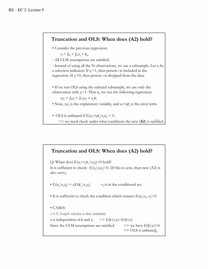
• Consider the previous regression:

yi= β0 + β1xi + εi,

- All CLM assumptions are satisfied.

- Instead of using all the N observations, we use a subsample. Let si be a selection indicator: If si=1, then person i is included in the regression. If si=0, then person i is dropped from the data.

• If we run OLS using the selected subsample, we use only the observation with si=1. That is, we run the following regression:

siyi= β0si + β1sixi + si εi• Now, sixi is the explanatory variable, and ui=siεi is the error term.

• OLS is unbiased if E(ui=siεi|sixi) = 0.

=> we need check under what conditions the new (A2) is satisfied.11

Truncation and OLS: When does (A2) hold?

Q: When does E(ui=si εi |sixi)=0 hold?

It is sufficient to check: E(ui|sixi)=0. (If this is zero, then new (A2) is also zero.)

• E(ui|xi,si) = siE(εi |xi,si) - si is in the conditional set.

• It is sufficient to check the condition which ensures E(ui|xi, si)=0.

• CASES:

(A-1) Sample selection is done randomly.

s is independent of ε and x. => E(ε|x,s)=E(ε|x).

Since the CLM assumptions are satisfied => we have E(ε|x)=0. => OLS is unbiased.

12



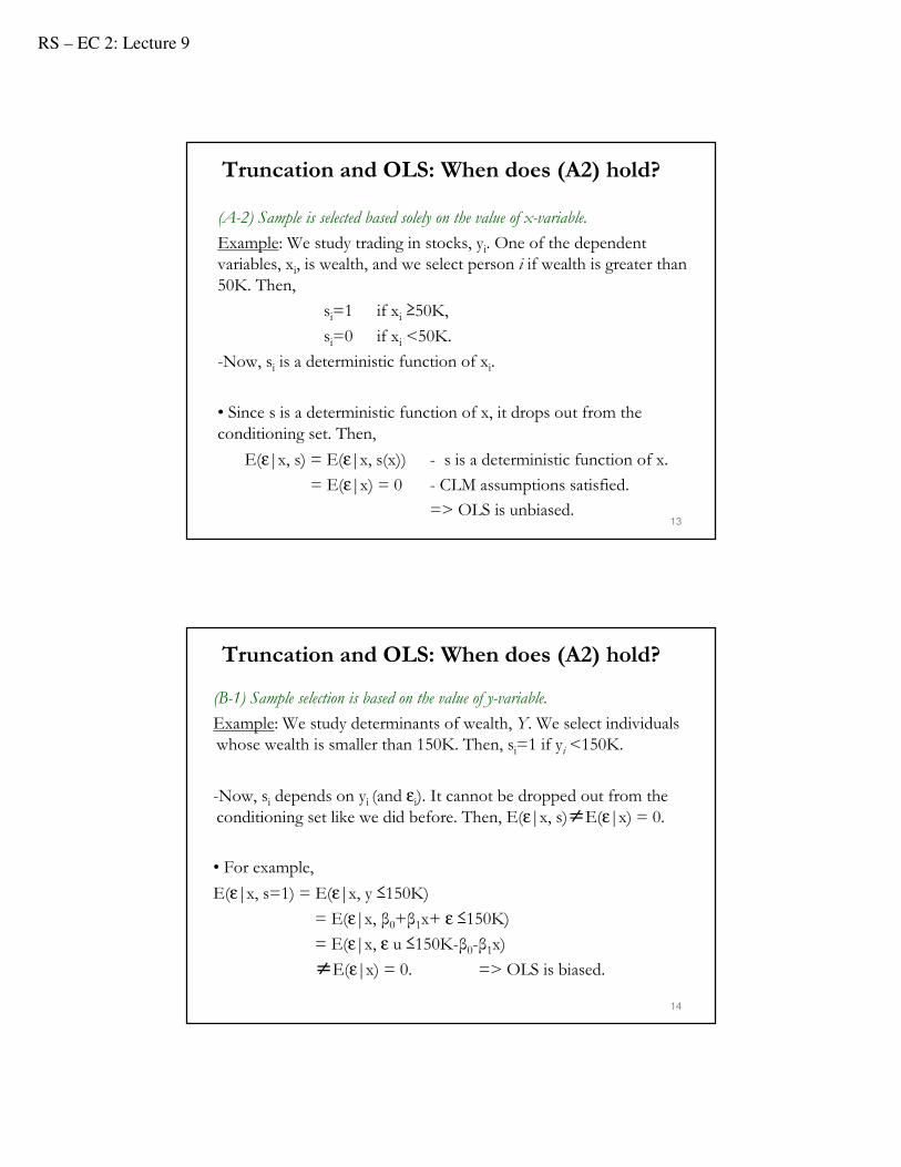
(A-2) Sample is selected based solely on the value of x-variable.

Example: We study trading in stocks, yi. One of the dependent variables, xi, is wealth, and we select person i if wealth is greater than 50K. Then,

si=1 if xi ≥50K,

si=0 if xi <50K.

-Now, si is a deterministic function of xi.

• Since s is a deterministic function of x, it drops out from the conditioning set. Then,

E(ε|x, s) = E(ε|x, s(x)) - s is a deterministic function of x.

= E(ε|x) = 0 - CLM assumptions satisfied.

=> OLS is unbiased. 13


(B-1) Sample selection is based on the value of y-variable.

Example: We study determinants of wealth, Y. We select individuals whose wealth is smaller than 150K. Then, si=1 if yi <150K.

-Now, si depends on yi (and εi). It cannot be dropped out from the conditioning set like we did before. Then, E(ε|x, s)≠E(ε|x) = 0.

• For example,

E(ε|x, s=1) = E(ε|x, y ≤150K)

= E(ε|x, β0+β1x+ ε ≤150K)

= E(ε|x, ε u ≤150K-β0-β1x)

≠E(ε|x) = 0. => OLS is biased.

14



(B-2) Sample selection is correlated with ui.

The inclusion of a person in the sample depends on the person’s decision, not the surveyor's decision. This type of truncation is called the incidental truncation. The bias that arises from this type of sample selection is called the Sample Selection Bias.

Example: wage offer regression of married women:

wagei = β0 + β1edui + εi.

Since it is the woman’s decision to participate, this sample selection is likely to be based on some unobservable factors which are contained in εi. Like in (B-1), s cannot be dropped out from the conditioning set:

E(ε|x, s) ≠E(ε|x) = 0 => OLS is biased. 15


• CASE (A-2) can be more complicated, when the selection rule based on the x-variable may be correlated with εi.

Example: X is IQ. A survey participant responds if IQ > v.

Now, the sample selection is based on x-variable and a random error v.

Q: If we run OLS using only the truncated data, will it cause a bias?

Two cases:

- (1) If v is independent of ε, then it does not cause a bias.

- (2) If v is correlated with ε, then this is the same case as (B-2). Then, OLS will be biased.

16



Estimation with Truncated Data.

• CASES

- Under cases (A-1) and (A-2), OLS is appropriate.

- Under case (B-1), we use Truncated regression.

- Under case (B-2) –i.e., incidental truncation-, we use the Heckman

Sample Selection Correction method. This is also called the Heckit model.

17

Truncated Regression

• Data truncation is (B-1): the truncation is based on the y-variable.

• We have the following regression satisfies all CLM assumptions:

yi= xi’ β + εi, εi~N(0, σ2)

- We sample only if yi< ci - Observations dropped if yi ≥ ci by design.

- We know the exact value of ci for each person.

• We know that OLS on the truncated data will cause biases. The model that produces unbiased estimate is based on the ML Estimation.

18


19

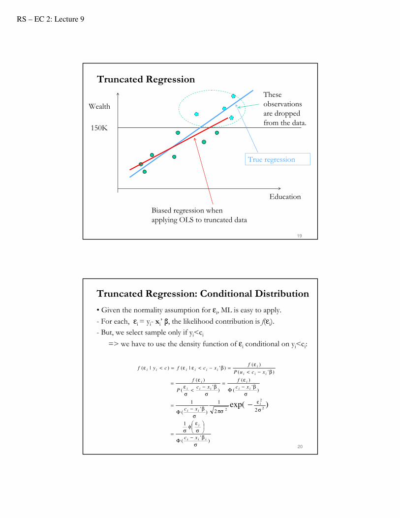
Wealth

Education

150K

These observations are dropped from the data.

True regression

Biased regression when applying OLS to truncated data

Truncated Regression

• Given the normality assumption for εi, ML is easy to apply.

- For each, εi = yi- xi’ β, the likelihood contribution is f(εi).

- But, we select sample only if yi<ci=> we have to use the density function of εi conditional on yi<ci:

20

Truncated Regression: Conditional Distribution

)'

(

1

22

1

)'

(

1

)'

(

)(

)'

(

)(

)'(

)()'|()|(

)exp(2

2

2

σ

β−Φ

σ

εφ

σ=

σ

ε

πσσ

β−Φ

=

σ

β−Φ

ε=

σ

β−<

σ

ε

ε=

β−<

ε=β−<εε=<ε

−

iii

i

i

ii

ii

i

iii

i

iii

iiiiiii

xc

xc

xc

f

xcP

f

xcuP

fxcfcyf


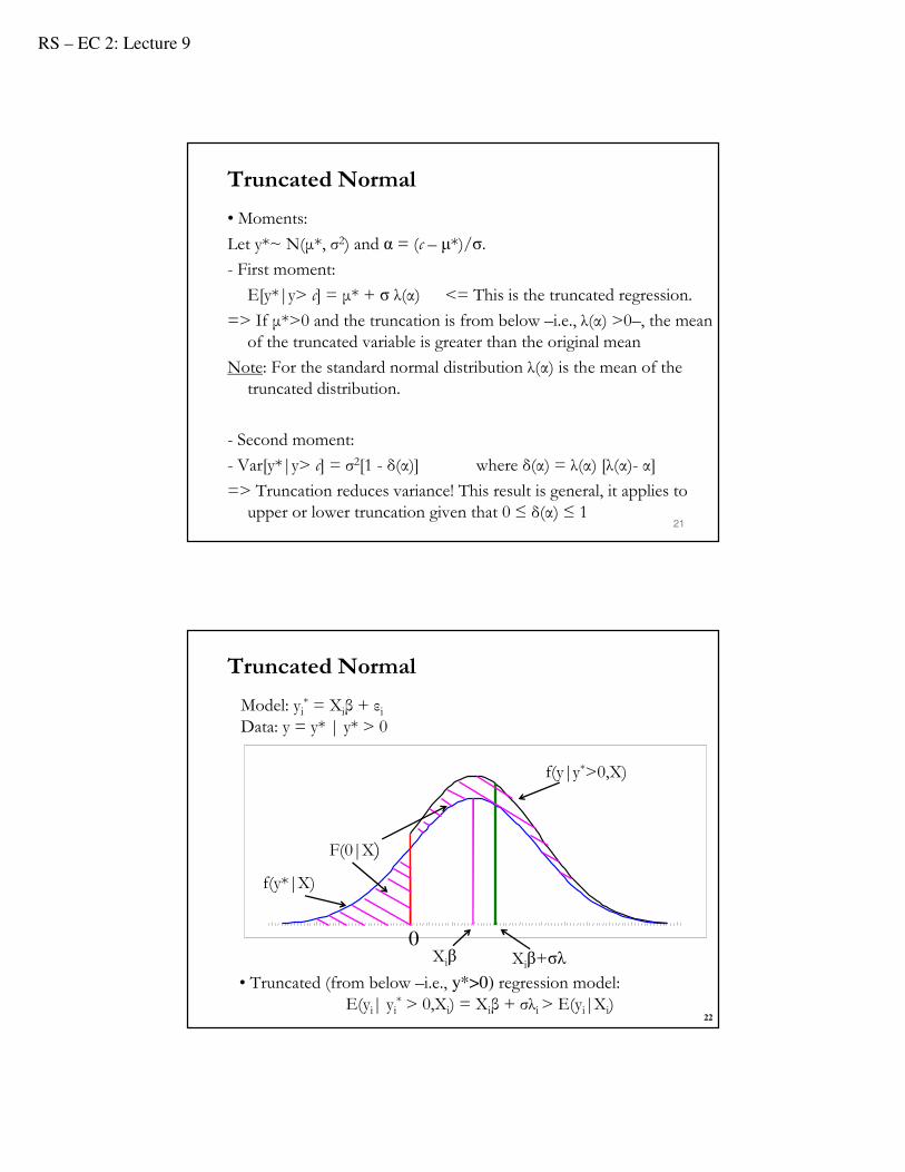
• Moments:

Let y*~ N(µ*, σ2) and α = (c – µ*)/σ.

- First moment:

E[y*|y> c] = µ* + σ λ(α) <= This is the truncated regression.

=> If µ*>0 and the truncation is from below –i.e., λ(α) >0–, the mean of the truncated variable is greater than the original mean

Note: For the standard normal distribution λ(α) is the mean of the truncated distribution.

- Second moment:

- Var[y*|y> c] = σ2[1 - δ(α)] where δ(α) = λ(α) [λ(α)- α]

=> Truncation reduces variance! This result is general, it applies to upper or lower truncation given that 0 ≤ δ(α) ≤ 1

21

Truncated Normal

22

f(y|y*>0,X)

F(0|X)

0Xiβ+σλ

Model: yi* = Xiβ + εi

Data: y = y* | y* > 0

• Truncated (from below –i.e., y*>0) regression model:E(yi| yi

* > 0,Xi) = Xiβ + σλi > E(yi|Xi)

Xiβ

f(y*|X)

Truncated Normal


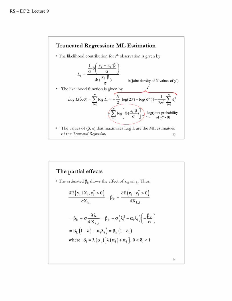
• The likelihood contribution for ith observation is given by

• The likelihood function is given by

• The values of (β, σ) that maximizes Log L are the ML estimators of the Truncated Regression. 23

)'

(

'1

σ

βΦ

σ

β−φ

σ=

i

ii

i x

xy

L

∑

∑∑

=

==

σ

βΦ−

εσ

−σ+π−==σβ

N

i

i

N

i

i

N

i

i

x

NLLLog

1

1

2

2

2

1

)'

(log

2

1)]log()2[log(

2log),(

Truncated Regression: ML Estimation

log(joint probability

of y*> 0)

ln(joint density of N values of y*)

The partial effects

• The estimated βk shows the effect of xki on yi. Thus,

24

( ) ( )

( )

( ) ( )

( ) ( )

* *i i i i i

kk ,i k ,i

2 kk k i i i

k ,i

2k i i i k i

i i i i i

E y | X , y 0 E | y 0

X X

X

1 1

where , 0 1

∂ > ∂ ε >= β +

∂ ∂

∂ λ β = β + σ = β + σ λ − α λ −

∂ σ

= β − λ − α λ = β − δ

δ = λ α λ α + α < δ <


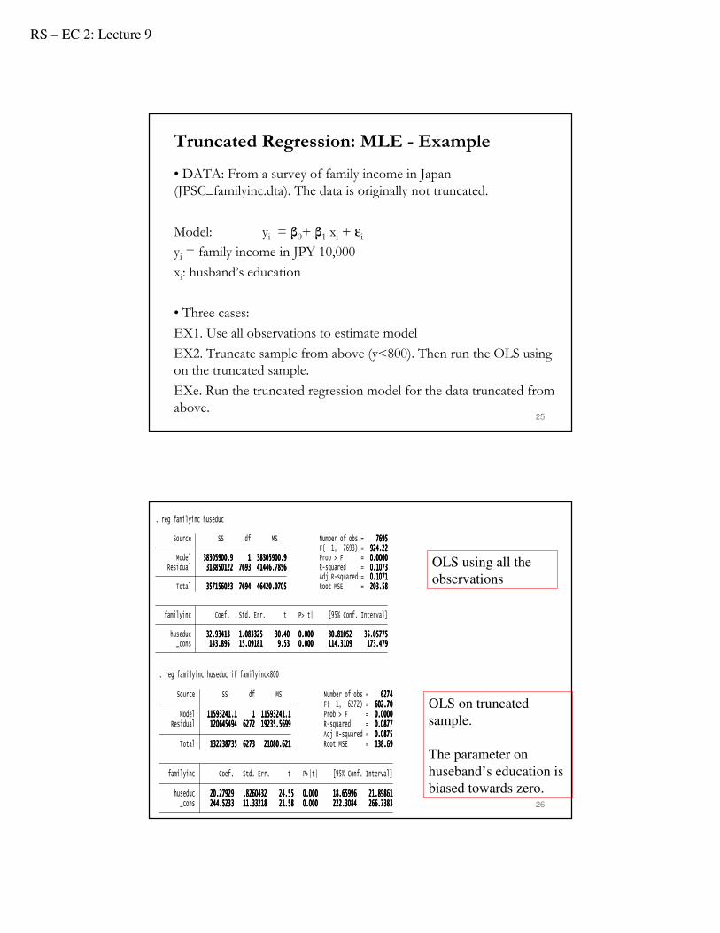
• DATA: From a survey of family income in Japan (JPSC_familyinc.dta). The data is originally not truncated.

Model: yi = β0+ β1 xi + εi yi = family income in JPY 10,000

xi: husband’s education

• Three cases:

EX1. Use all observations to estimate model

EX2. Truncate sample from above (y<800). Then run the OLS using on the truncated sample.

EXe. Run the truncated regression model for the data truncated fromabove.

25

Truncated Regression: MLE - Example

26

_cons 111144443333....888899995555 11115555....00009999111188881111 9999....55553333 0000....000000000000 111111114444....3333111100009999 111177773333....444477779999 huseduc 33332222....99993333444411113333 1111....000088883333333322225555 33330000....44440000 0000....000000000000 33330000....88881111000055552222 33335555....00005555777777775555 familyinc Coef. Std. Err. t P>|t| [95% Conf. Interval]

Total 333355557777111155556666000022223333 7777666699994444 44446666444422220000....0000777700005555 Root MSE = 222200003333....55558888 Adj R-squared = 0000....1111000077771111 Residual 333311118888888855550000111122222222 7777666699993333 44441111444444446666....7777888855556666 R-squared = 0000....1111000077773333 Model 33338888333300005555999900000000....9999 1111 33338888333300005555999900000000....9999 Prob > F = 0000....0000000000000000 F( 1, 7693) = 999922224444....22222222 Source SS df MS Number of obs = 7777666699995555

. reg familyinc huseduc

_cons 222244444444....5555222233333333 11111111....33333333222211118888 22221111....55558888 0000....000000000000 222222222222....3333000088884444 222266666666....7777333388883333 huseduc 22220000....22227777999922229999 ....8888222266660000444433332222 22224444....55555555 0000....000000000000 11118888....66665555999999996666 22221111....88889999888866661111 familyinc Coef. Std. Err. t P>|t| [95% Conf. Interval]

Total 111133332222222233338888777733335555 6666222277773333 22221111000088880000....666622221111 Root MSE = 111133338888....66669999 Adj R-squared = 0000....0000888877775555 Residual 111122220000666644445555444499994444 6666222277772222 11119999222233335555....5555666699999999 R-squared = 0000....0000888877777777 Model 11111111555599993333222244441111....1111 1111 11111111555599993333222244441111....1111 Prob > F = 0000....0000000000000000 F( 1, 6272) = 666600002222....77770000 Source SS df MS Number of obs = 6666222277774444

. reg familyinc huseduc if familyinc<800

OLS using all the

observations

OLS on truncated

sample.

The parameter on

huseband’s education is

biased towards zero.


27

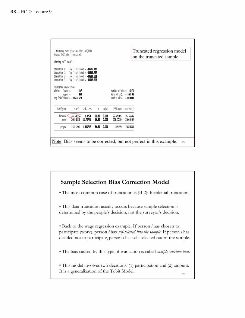
/sigma 111155553333....1111222299991111 1111....888800005555777711117777 88884444....88880000 0000....000000000000 111144449999....55559999 111155556666....6666666688883333 _cons 222200003333....6666888855556666 11113333....77775555777722221111 11114444....88881111 0000....000000000000 111177776666....7777222211119999 222233330000....6666444499992222 huseduc 22224444....55550000222277776666 1111....0000222266664444 22223333....88887777 0000....000000000000 22222222....44449999111100005555 22226666....55551111444444446666 familyinc Coef. Std. Err. z P>|z| [95% Conf. Interval]

Log likelihood = ----33339999666611118888....666622229999 Prob > chi2 = 0000....0000000000000000 upper = 888800000000 Wald chi2(1111) = 555566669999....99990000Limit: lower = ----iiiinnnnffff Number of obs = 6666222277774444Truncated regression

Iteration 3: log likelihood = ----33339999666611118888....666622229999 Iteration 2: log likelihood = ----33339999666611118888....666622229999 Iteration 1: log likelihood = ----33339999666611118888....777755557777 Iteration 0: log likelihood = ----33339999666677776666....777788882222

Fitting full model:

(note: 1421 obs. truncated). truncreg familyinc huseduc, ul(800) Truncated regression model

on the truncated sample

Note: Bias seems to be corrected, but not perfect in this example.

Sample Selection Bias Correction Model

• The most common case of truncation is (B-2): Incidental truncation.

• This data truncation usually occurs because sample selection isdetermined by the people’s decision, not the surveyor’s decision.

• Back to the wage regression example. If person i has chosen to participate (work), person i has self-selected into the sample. If person i has decided not to participate, person i has self-selected out of the sample.

• The bias caused by this type of truncation is called sample selection bias.

• This model involves two decisions: (1) participation and (2) amount. It is a generalization of the Tobit Model.

28


29

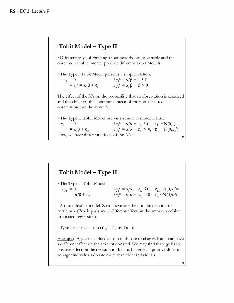
• Different ways of thinking about how the latent variable and the observed variable interact produce different Tobit Models.

• The Type I Tobit Model presents a simple relation:- yi = 0 if yi* = xi’β + εi ≤ 0

= yi* = xi’β + εi if yi* = xi’β + εi > 0

The effect of the X’s on the probability that an observation is censored and the effect on the conditional mean of the non-censored observations are the same: β.

• The Type II Tobit Model presents a more complex relation:- yi = 0 if yi* = xi’α + ε1,i ≤ 0, ε1,i ~N(0,1)

= xi’β + ε2,i if yi* = xi’α + ε1,i > 0, ε2,i ~N(0,σ22)

Now, we have different effects of the X’s.

Tobit Model – Type II

30

• The Type II Tobit Model:- yi = 0 if yi* = xi’α + ε1,i ≤ 0, ε1,i~N(0,σ1

2=1)= xi’β + ε2,i if yi* = xi’α + ε1,i > 0, ε2,i~N(0,σ2

2)

- A more flexible model. X can have an effect on the decision to participate (Probit part) and a different effect on the amount decision (truncated regression).

- Type I is a special case: ε2,i = ε1,i and α=β.

Example: Age affects the decision to donate to charity. But it can have a different effect on the amount donated. We may find that age has a positive effect on the decision to donate, but given a positive donation, younger individuals donate more than older individuals.



31

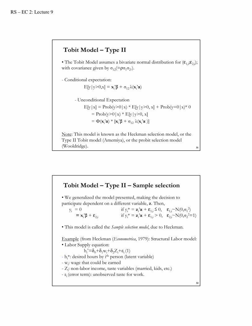
• The Tobit Model assumes a bivariate normal distribution for (ε1,i;ε2,i); with covariance given by σ12(=ρσ1σ2.).

- Conditional expectation:

E[y|y>0,x] = xi’β + σ12 λ(xi’α)

- Unconditional Expectation

E[y|x] = Prob(y>0|x) * E[y|y>0, x] + Prob(y=0|x)* 0

= Prob(y>0|x) * E[y|y>0, x]

= Φ(xi’α) * [xi’β + σ12 λ(xi’α )]

Note: This model is known as the Heckman selection model, or the Type II Tobit model (Amemiya), or the probit selection model (Wooldridge).


32

• We generalized the model presented, making the decision to participate dependent on a different variable, z. Then,

yi = 0 if yi* = zi’α + ε1,i ≤ 0, ε1,i~N(0,σ12)

= xi’β + ε2,i if yi* = zi’α + ε1,i > 0, ε2,i~N(0,σ22=1)

• This model is called the Sample selection model, due to Heckman.

Example (from Heckman (Econometrica, 1979): Structural Labor model:• Labor Supply equation:

hi*=δ0+δ1wi+δ2Zi+εi (1)

- hi*: desired hours by ith person (latent variable)

- wi: wage that could be earned - Zi: non-labor income, taste variables (married, kids, etc.)- εi (error term): unobserved taste for work.

Tobit Model – Type II – Sample selection


33

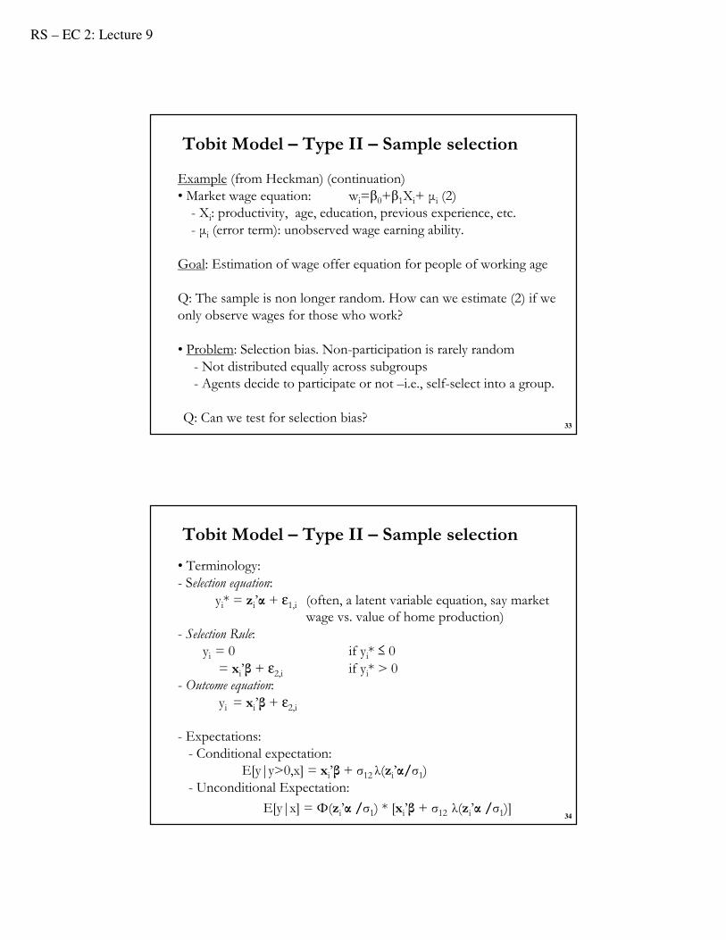
Example (from Heckman) (continuation)• Market wage equation: wi=β0+β1Xi+ µi (2) - Xi: productivity, age, education, previous experience, etc.- µi (error term): unobserved wage earning ability.

Goal: Estimation of wage offer equation for people of working age

Q: The sample is non longer random. How can we estimate (2) if we only observe wages for those who work?

• Problem: Selection bias. Non-participation is rarely random- Not distributed equally across subgroups- Agents decide to participate or not –i.e., self-select into a group.

Q: Can we test for selection bias?


34

• Terminology: - Selection equation:

yi* = zi’α + ε1,i (often, a latent variable equation, say market wage vs. value of home production)

- Selection Rule:yi = 0 if yi* ≤ 0= xi’β + ε2,i if yi* > 0

- Outcome equation:yi = xi’β + ε2,i

- Expectations:- Conditional expectation:

E[y|y>0,x] = xi’β + σ12 λ(zi’α/σ1) - Unconditional Expectation:

E[y|x] = Φ(zi’α /σ1) * [xi’β + σ12 λ(zi’α /σ1)]



35

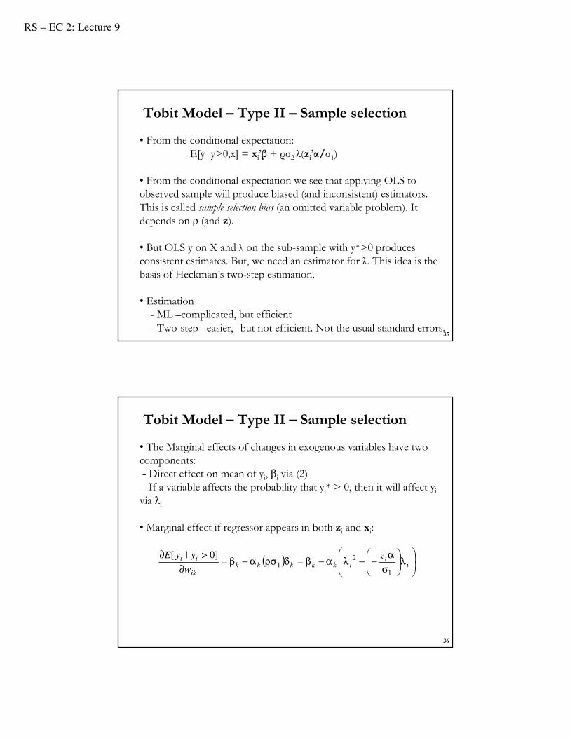
• From the conditional expectation:E[y|y>0,x] = xi’β + ρσ2 λ(zi’α/σ1)

• From the conditional expectation we see that applying OLS to observed sample will produce biased (and inconsistent) estimators. This is called sample selection bias (an omitted variable problem). It depends on ρ (and z).

• But OLS y on X and λ on the sub-sample with y*>0 produces consistent estimates. But, we need an estimator for λ. This idea is the basis of Heckman’s two-step estimation.

• Estimation- ML –complicated, but efficient- Two-step –easier, but not efficient. Not the usual standard errors.


36

• The Marginal effects of changes in exogenous variables have two components:- Direct effect on mean of yi, βi via (2)- If a variable affects the probability that yi* > 0, then it will affect yivia λi

• Marginal effect if regressor appears in both zi and xi:


( )

λ

σ

α−−λα−β=δρσα−β=

∂

>∂i

iikkkkk

ik

ii z

w

yyE

1

21

]0|[


( )( )

( )1 2

1 212

2 2

,f x xf x x

f x=

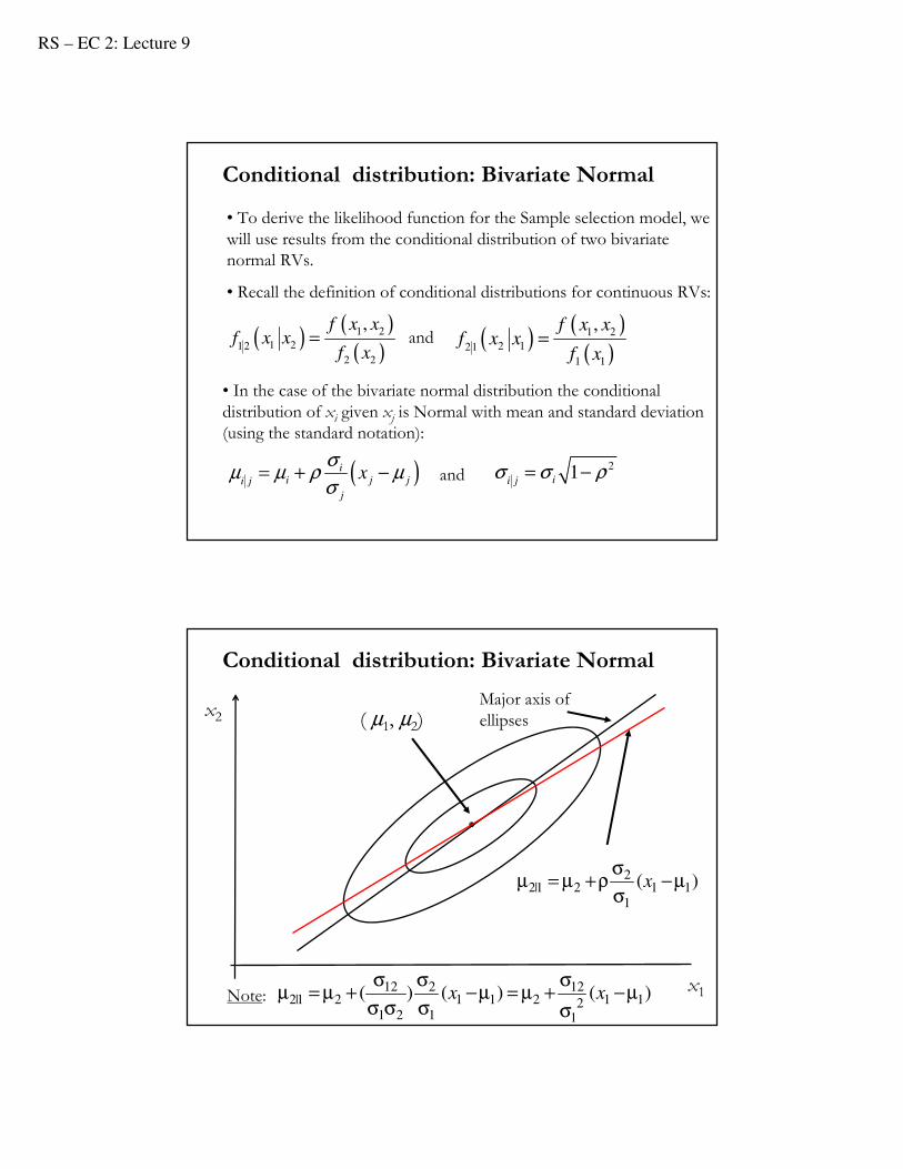
Conditional distribution: Bivariate Normal

• To derive the likelihood function for the Sample selection model, we will use results from the conditional distribution of two bivariate normal RVs.

• Recall the definition of conditional distributions for continuous RVs:

and

• In the case of the bivariate normal distribution the conditional distribution of xi given xj is Normal with mean and standard deviation (using the standard notation):

( )( )

( )1 2

2 121

1 1

,f x xf x x

f x=

and( )ii j ji j

j

xσ

µ µ ρ µσ

= + − 21ii j

σ σ ρ= −

( µ1, µ2)x2

x1

Major axis of ellipses

)( 111

221|2 µ−

σ

σρ+µ=µ x

Note: )()()( 1121

12211

1

2

21

1221|2 µ−

σ

σ+µ=µ−

σ

σ

σσ

σ+µ=µ xx

Conditional distribution: Bivariate Normal


39

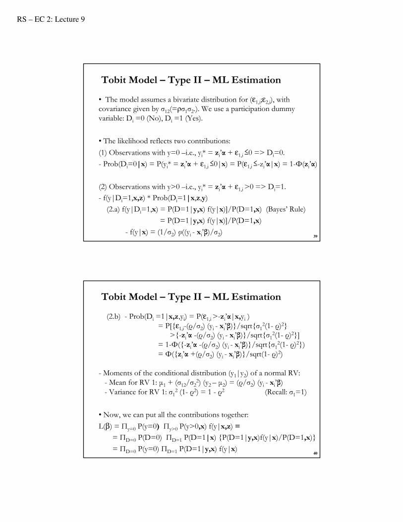
• The model assumes a bivariate distribution for (ε1,i;ε2,i), with covariance given by σ12(=ρσ1σ2.). We use a participation dummy variable: Di =0 (No), Di =1 (Yes).

• The likelihood reflects two contributions:

(1) Observations with y=0 –i.e., yi* = zi’α + ε1,i ≤0 => Di=0.

- Prob(Di=0|x) = P(yi* = zi’α + ε1,i ≤0|x) = P(ε1,i ≤-zi’α|x) = 1-Φ(zi’α)

(2) Observations with y>0 –i.e., yi* = zi’α + ε1,i >0 => Di=1.

- f(y|Di=1,x,z) * Prob(Di=1|x,z,y)

(2.a) f(y|Di=1,x) = P(D=1|y,x) f(y|x)]/P(D=1,x) (Bayes’ Rule)

= P(D=1|y,x) f(y|x)]/P(D=1,x)

- f(y|x) = (1/σ2) φ((yi - xi’β)/σ2)

Tobit Model – Type II – ML Estimation

40

(2.b) - Prob(Di =1|x,z,yi) = P(ε1,i >-zi’α|x,yi ) = P[{ε1,i-(ρ/σ2) (yi - xi’β)}/sqrt{σ1

2(1- ρ)2}>{-zi’α -(ρ/σ2) (yi - xi’β)}/sqrt{σ1

2(1- ρ)2}] = 1-Φ({-zi’α -(ρ/σ2) (yi - xi’β)}/sqrt{σ1

2(1- ρ)2})= Φ({zi’α +(ρ/σ2) (yi - xi’β)}/sqrt(1- ρ)

2)

- Moments of the conditional distribution (y1|y2) of a normal RV: - Mean for RV 1: µ1 + (σ12/σ2

2) (y2 – µ2) = (ρ/σ2) (yi - xi’β) - Variance for RV 1: σ1

2 (1- ρ2) = 1 - ρ2 (Recall: σ1=1)

• Now, we can put all the contributions together:

L(β) = Πy=0 P(y=0) Πy>0 P(y>0,x) f(y|x,z) =

= ΠD=0 P(D=0) ΠD=1 P(D=1|x) {P(D=1|y,x)f(y|x)/P(D=1,x)}

= ΠD=0 P(y=0) ΠD=1 P(D=1|y,x) f(y|x)



41

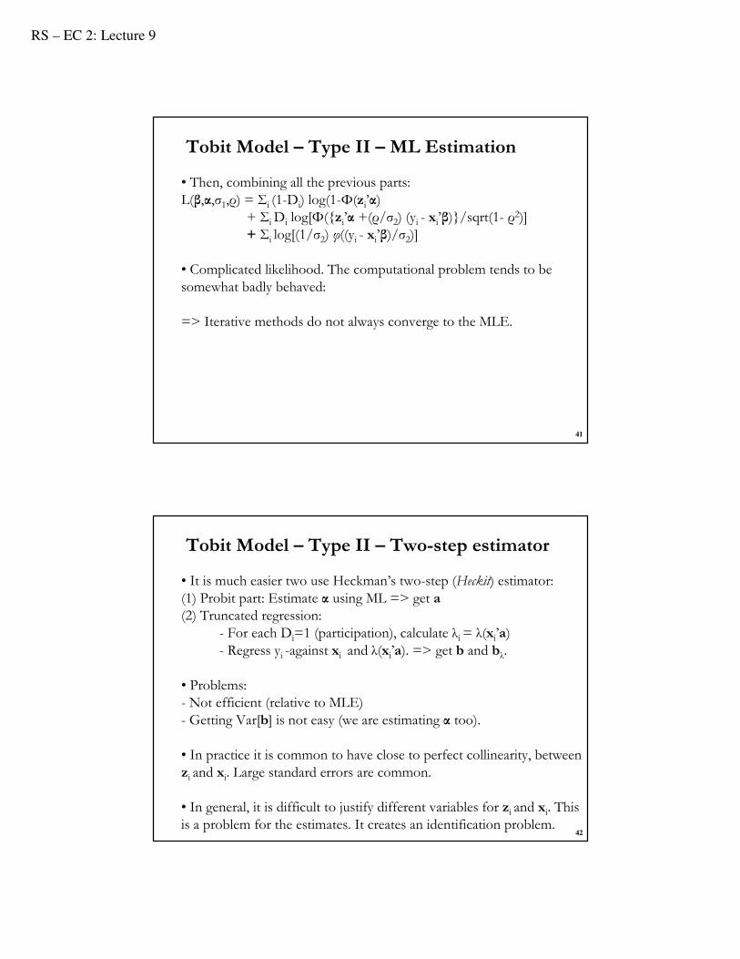
• Then, combining all the previous parts: L(β,α,σ1,ρ) = Σi (1-Di) log(1-Φ(zi’α)

+ Σi Di log[Φ({zi’α +(ρ/σ2) (yi - xi’β)}/sqrt(1- ρ2)]

+ Σi log[(1/σ2) φ((yi - xi’β)/σ2)]

• Complicated likelihood. The computational problem tends to be somewhat badly behaved:

=> Iterative methods do not always converge to the MLE.


42

• It is much easier two use Heckman’s two-step (Heckit) estimator:(1) Probit part: Estimate α using ML => get a(2) Truncated regression:

- For each Di=1 (participation), calculate λi = λ(xi’a) - Regress yi -against xi and λ(xi’a). => get b and bλ.

• Problems: - Not efficient (relative to MLE) - Getting Var[b] is not easy (we are estimating α too).

• In practice it is common to have close to perfect collinearity, between zi and xi. Large standard errors are common.

• In general, it is difficult to justify different variables for zi and xi. This is a problem for the estimates. It creates an identification problem.

Tobit Model – Type II – Two-step estimator


43

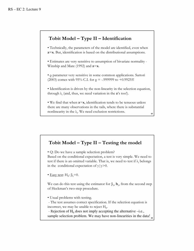
• Technically, the parameters of the model are identified, even when z=x. But, identification is based on the distributional assumptions.

• Estimates are very sensitive to assumption of bivariate normality -Winship and Mare (1992) and z=x.

• ρ parameter very sensitive in some common applications. Sartori(2003) comes with 95% C.I. for ρ = -.999999 to +0.99255!

• Identification is driven by the non-linearity in the selection equation, through λi (and, thus, we need variation in the z’s too!).

• We find that when z=x, identification tends to be tenuous unless there are many observations in the tails, where there is substantial nonlinearity in the λi. We need exclusion restrictions.

Tobit Model – Type II – Identification

44

• Q: Do we have a sample selection problem?Based on the conditional expectation, a test is very simple. We need to test if there is an omitted variable. That is, we need to test if λi belongs in the conditional expectation of y|y>0.

• Easy test: H0: βλ=0.

We can do this test using the estimator for βλ, bλ, from the second step of Heckman’s two-step procedure.

• Usual problems with testing. - The test assumes correct specification. If the selection equation is incorrect, we may be unable to reject H0.- Rejection of H0 does not imply accepting the alternative –i.e.,

sample selection problem. We may have non-linearities in the data!

Tobit Model – Type II – Testing the model


45

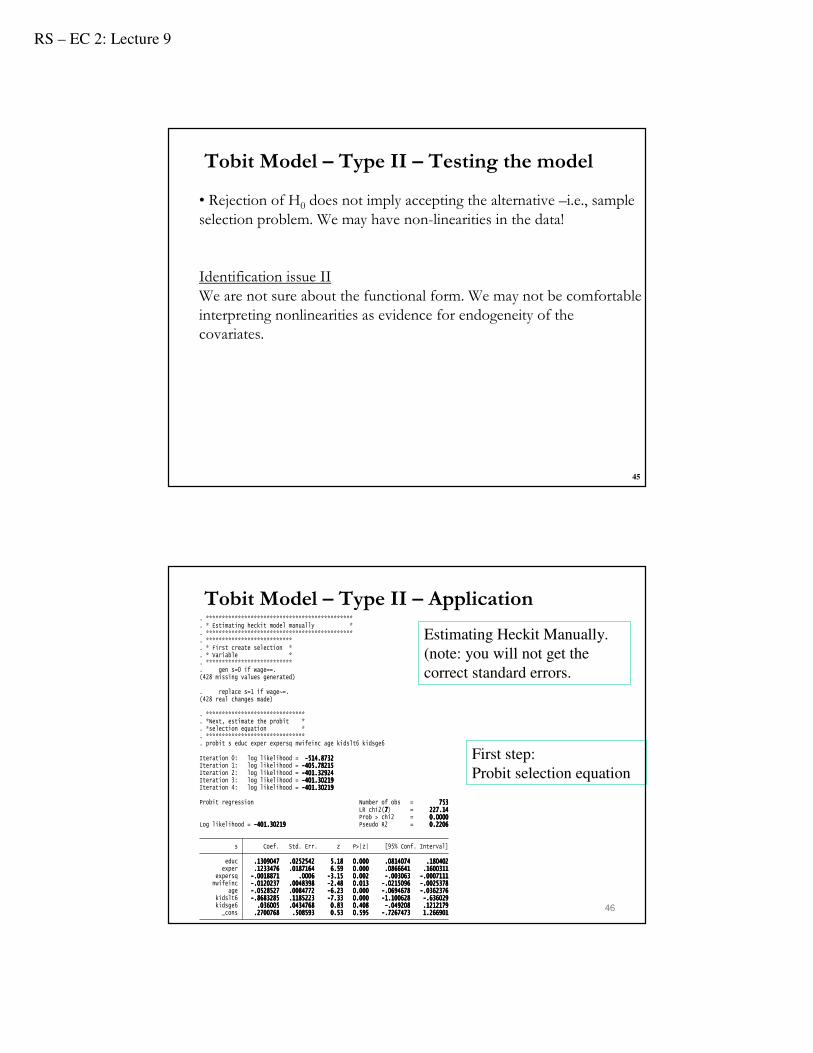
• Rejection of H0 does not imply accepting the alternative –i.e., sample selection problem. We may have non-linearities in the data!

Identification issue IIWe are not sure about the functional form. We may not be comfortable interpreting nonlinearities as evidence for endogeneity of the covariates.

Tobit Model – Type II – Testing the model

46

_cons ....2222777700000000777766668888 ....555500008888555599993333 0000....55553333 0000....555599995555 ----....7777222266667777444477773333 1111....222266666666999900001111 kidsge6 ....000033336666000000005555 ....0000444433334444777766668888 0000....88883333 0000....444400008888 ----....000044449999222200008888 ....1111222211112222111177779999 kidslt6 ----....8888666688883333222288885555 ....1111111188885555222222223333 ----7777....33333333 0000....000000000000 ----1111....111100000000666622228888 ----....666633336666000022229999 age ----....0000555522228888555522227777 ....0000000088884444777777772222 ----6666....22223333 0000....000000000000 ----....0000666699994444666677778888 ----....0000333366662222333377776666 nwifeinc ----....0000111122220000222233337777 ....0000000044448888333399998888 ----2222....44448888 0000....000011113333 ----....0000222211115555000099996666 ----....0000000022225555333377778888 expersq ----....0000000011118888888877771111 ....0000000000006666 ----3333....11115555 0000....000000002222 ----....000000003333000066663333 ----....0000000000007777111111111111 exper ....1111222233333333444477776666 ....0000111188887777111166664444 6666....55559999 0000....000000000000 ....0000888866666666666644441111 ....1111666600000000333311111111 educ ....1111333300009999000044447777 ....0000222255552222555544442222 5555....11118888 0000....000000000000 ....0000888811114444000077774444 ....111188880000444400002222 s Coef. Std. Err. z P>|z| [95% Conf. Interval]

Log likelihood = ----444400001111....33330000222211119999 Pseudo R2 = 0000....2222222200006666 Prob > chi2 = 0000....0000000000000000 LR chi2(7777) = 222222227777....11114444Probit regression Number of obs = 777755553333

Iteration 4: log likelihood = ----444400001111....33330000222211119999Iteration 3: log likelihood = ----444400001111....33330000222211119999Iteration 2: log likelihood = ----444400001111....33332222999922224444Iteration 1: log likelihood = ----444400005555....77778888222211115555Iteration 0: log likelihood = ----555511114444....8888777733332222

. probit s educ exper expersq nwifeinc age kidslt6 kidsge6

. *******************************

. *selection equation *

. *Next, estimate the probit *

. *******************************

(428 real changes made). replace s=1 if wage~=.

(428 missing values generated). gen s=0 if wage==.. ***************************. * Variable *. * First create selection *. ***************************. **********************************************. * Estimating heckit model manually *. **********************************************

Estimating Heckit Manually.

(note: you will not get the

correct standard errors.

First step:

Probit selection equation

Tobit Model – Type II – Application


47

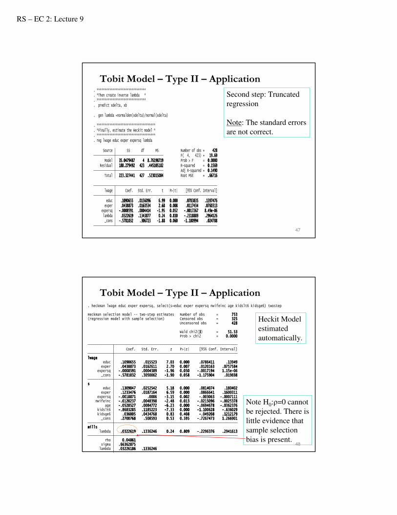
_cons ----....5555777788881111000033332222 ....333300006666777722223333 ----1111....88888888 0000....000066660000 ----1111....111188880000999999994444 ....000022224444777788888888 lambda ....0000333322222222666611119999 ....1111333344443333888877777777 0000....22224444 0000....888811110000 ----....2222333311118888888888889999 ....2222999966664444111122226666 expersq ----....0000000000008888555599991111 ....0000000000004444444411114444 ----1111....99995555 0000....000055552222 ----....0000000011117777222266667777 8888....44449999eeee----00006666 exper ....0000444433338888888877773333 ....0000111166663333555533334444 2222....66668888 0000....000000008888 ....0000111111117777444433334444 ....0000777766660000333311113333 educ ....1111000099990000666655555555 ....0000111155556666000099996666 6666....99999999 0000....000000000000 ....0000777788883333888833335555 ....1111333399997777444477776666 lwage Coef. Std. Err. t P>|t| [95% Conf. Interval]

Total 222222223333....333322227777444444441111 444422227777 ....555522223333000011115555000088884444 Root MSE = ....66666666777711116666 Adj R-squared = 0000....1111444499990000 Residual 111188888888....222277779999444499992222 444422223333 ....444444445555111100005555111188882222 R-squared = 0000....1111555566669999 Model 33335555....0000444477779999444488887777 4444 8888....77776666111199998888777711119999 Prob > F = 0000....0000000000000000 F( 4, 423) = 11119999....66669999 Source SS df MS Number of obs = 444422228888

. reg lwage educ exper expersq lambda

. *************************************

. *Finally, estimate the Heckit model *

. *************************************

. gen lambda =normalden(xdelta)/normal(xdelta)

. predict xdelta, xb

. *******************************

. *Then create inverse lambda *

. *******************************Second step: Truncated

regression

Note: The standard errors

are not correct.


48

lambda ....00003333222222226666111188886666 ....1111333333336666222244446666 sigma ....66666666333366662222888877775555 rho 0000....00004444888866661111 lambda ....0000333322222222666611119999 ....1111333333336666222244446666 0000....22224444 0000....888800009999 ----....2222222299996666333377776666 ....2222999944441111666611113333mmmmiiiillllllllssss _cons ....2222777700000000777766668888 ....555500008888555599993333 0000....55553333 0000....555599995555 ----....7777222266667777444477773333 1111....222266666666999900001111 kidsge6 ....000033336666000000005555 ....0000444433334444777766668888 0000....88883333 0000....444400008888 ----....000044449999222200008888 ....1111222211112222111177779999 kidslt6 ----....8888666688883333222288885555 ....1111111188885555222222223333 ----7777....33333333 0000....000000000000 ----1111....111100000000666622228888 ----....666633336666000022229999 age ----....0000555522228888555522227777 ....0000000088884444777777772222 ----6666....22223333 0000....000000000000 ----....0000666699994444666677778888 ----....0000333366662222333377776666 nwifeinc ----....0000111122220000222233337777 ....0000000044448888333399998888 ----2222....44448888 0000....000011113333 ----....0000222211115555000099996666 ----....0000000022225555333377778888 expersq ----....0000000011118888888877771111 ....0000000000006666 ----3333....11115555 0000....000000002222 ----....000000003333000066663333 ----....0000000000007777111111111111 exper ....1111222233333333444477776666 ....0000111188887777111166664444 6666....55559999 0000....000000000000 ....0000888866666666666644441111 ....1111666600000000333311111111 educ ....1111333300009999000044447777 ....0000222255552222555544442222 5555....11118888 0000....000000000000 ....0000888811114444000077774444 ....111188880000444400002222ssss _cons ----....5555777788881111000033332222 ....3333000055550000000066662222 ----1111....99990000 0000....000055558888 ----1111....111177775555999900004444 ....000011119999666699998888 expersq ----....0000000000008888555599991111 ....0000000000004444333388889999 ----1111....99996666 0000....000055550000 ----....0000000011117777111199994444 1111....11115555eeee----00006666 exper ....0000444433338888888877773333 ....0000111166662222666611111111 2222....77770000 0000....000000007777 ....0000111122220000111166663333 ....0000777755557777555588884444 educ ....1111000099990000666655555555 ....000011115555555522223333 7777....00003333 0000....000000000000 ....0000777788886666444411111111 ....11113333999944449999llllwwwwaaaaggggeeee Coef. Std. Err. z P>|z| [95% Conf. Interval]

Prob > chi2 = 0000....0000000000000000 Wald chi2(3333) = 55551111....55553333

Uncensored obs = 444422228888(regression model with sample selection) Censored obs = 333322225555Heckman selection model -- two-step estimates Number of obs = 777755553333

. heckman lwage educ exper expersq, select(s=educ exper expersq nwifeinc age kidslt6 kidsge6) twostep

Heckit Model

estimated

automatically.

Note H0:ρ=0 cannot

be rejected. There is

little evidence that

sample selection

bias is present.


Truncated Regression and Sample Selection

Documents

Transcript of Truncated Regression and Sample Selection