Truncated Back-propagation for Bilevel Optimization

Amirreza Shaban* Ching-An Cheng* Nathan Hatch Byron BootsGeorgia Institute of Technology *Equal contribution

Abstract

Bilevel optimization has been recently revis-ited for designing and analyzing algorithmsin hyperparameter tuning and meta learn-ing tasks. However, due to its nested struc-ture, evaluating exact gradients for high-dimensional problems is computationally chal-lenging. One heuristic to circumvent this di�-culty is to use the approximate gradient givenby performing truncated back-propagationthrough the iterative optimization procedurethat solves the lower-level problem. Althoughpromising empirical performance has been re-ported, its theoretical properties are still un-clear. In this paper, we analyze the propertiesof this family of approximate gradients andestablish su�cient conditions for convergence.We validate this on several hyperparametertuning and meta learning tasks. We find thatoptimization with the approximate gradientcomputed using few-step back-propagationoften performs comparably to optimizationwith the exact gradient, while requiring farless memory and half the computation time.

1 INTRODUCTION

Bilevel optimization has been recently revisited as atheoretical framework for designing and analyzing algo-rithms for hyperparameter optimization [1] and metalearning [2]. Mathematically, these problems can beformulated as a stochastic optimization problem withan equality constraint (see Section 1.1):

min�

F (�) := ES [fS(w⇤S(�),�)]

s.t. w⇤S(�) ⇡� argmin

wgS(w,�)

(1)

where w and � are the parameter and the hyperpa-rameter, F and fS are the expected and the sampled

Proceedings of the 22nd International Conference on Ar-tificial Intelligence and Statistics (AISTATS) 2019, Naha,Okinawa, Japan. PMLR: Volume 89. Copyright 2019 bythe author(s).

upper-level objective, gS is the sampled lower-level ob-jective, and S is a random variable called the context.The notation ⇡� means that w⇤

S(�) equals the uniquereturn value of a prespecified iterative algorithm (e.g.gradient descent) that approximately finds a local min-imum of gS . This algorithm is part of the problemdefinition and can also be parametrized by � (e.g. stepsize). The motivation to explicitly consider the approxi-mate solution w⇤

S(�) rather than an exact minimizer w⇤S

of gS is that w⇤S is usually not available in closed form.

This setup enables � to account for the imperfectionsof the lower-level optimization algorithm.

Solving the bilevel optimization problem in (1) is chal-lenging due to the complicated dependency of theupper-level problem on � induced by w⇤

S(�). Thisdi�culty is further aggravated when � and w are high-dimensional, precluding the use of black-box optimiza-tion techniques such as grid/random search [3] andBayesian optimization [4, 5].

Recently, first-order bilevel optimization techniqueshave been revisited to solve these problems. Thesemethods rely on an estimate of the Jacobian r�w⇤

S(�)to optimize �. Pedregosa [6] and Gould et al. [7] assumethat w⇤

S(�) = w⇤S and compute r�w⇤

S(�) by implicitdi↵erentiation. By contrast, Maclaurin et al. [8] andFranceschi et al. [9] treat the iterative optimizationalgorithm in the lower-level problem as a dynamicalsystem, and compute r�w⇤

S(�) by automatic di↵eren-tiation through the dynamical system. In comparison,the latter approach is less sensitive to the optimality ofw⇤

S(�) and can also learn hyperparameters that controlthe lower-level optimization process (e.g. step size).However, due to superlinear time or space complexity(see Section 2.2), neither of these methods is applicablewhen both � and w are high-dimensional [9].

Few-step reverse-mode automatic di↵erentiation [10,11] and few-step forward-mode automatic di↵erentia-tion [9] have recently been proposed as heuristics toaddress this issue. By ignoring long-term dependencies,the time and space complexities to compute approxi-mate gradients can be greatly reduced. While excitingempirical results have been reported, the theoreticalproperties of these methods remain unclear.

Truncated Back-propagation for Bilevel Optimization

In this paper, we study the theoretical propertiesof these truncated back-propagation approaches. Weshow that, when the lower-level problem is locallystrongly convex around w⇤

S(�), on-average convergenceto an ✏-approximate stationary point is guaranteedby O(log 1/✏)-step truncated back-propagation. Wealso identify additional problem structures for whichasymptotic convergence to an exact stationary point isguaranteed. Empirically, we verify the utility of thisstrategy for hyperparameter optimization and metalearning tasks. We find that, compared to optimizationwith full back-propagation, optimization with trun-cated back-propagation usually shows competitive per-formance while requiring half as much computationtime and significantly less memory.

1.1 Applications

Hyperparameter Optimization The goal of hy-perparameter optimization [12, 13] is to find hyperpa-rameters � for an optimization problem P such that theapproximate solution w⇤(�) of P has low cost c(w⇤(�))for some cost function c. In general, � can parametrizeboth the objective of P and the algorithm used tosolve P . This setup is a special case of the bilevel opti-mization problem (1) where the upper-level objectivec does not depend directly on �. In contrast to metalearning (discussed below), c can be deterministic [9].See Section 4.2 for examples.

Many low-dimensional problems, such as choosing thelearning rate and regularization constant for trainingneural networks, can be e↵ectively solved with gridsearch. However, problems with thousands of hyperpa-rameters are increasingly common, for which gradient-based methods are more appropriate [8, 14].

Meta Learning Another important application ofbilevel optimization, meta learning (or learning-to-learn) uses statistical learning to optimize an algorithmA� over a distribution of tasks T and contexts S:

min�

ET ES|T [cT (A�(S))] . (2)

It treats A� as a parametric function, with hyperpa-rameter �, that takes task-specific context informationS as input and outputs a decision A�(S). The goalof meta learning is to optimize the algorithm’s perfor-mance cT (e.g. the generalization error) across tasksT through empirical observations. This general setupsubsumes multiple problems commonly encounteredin the machine learning literature, such as multi-tasklearning [15, 16] and few-shot learning [17, 18, 19].

Bilevel optimization emerges from meta learning whenthe algorithm computes A�(S) by internally solvinga lower-level minimization problem with variable w.The motivation to use this class of algorithms is that

the lower-level problem can be designed so that, evenfor tasks T distant from the training set, A� fallsback upon a sensible optimization-based approach [20,11]. By contrast, treating A� as a general functionapproximator relies on the availability of a large amountof meta training data [21, 22].

In other words, the decision is A�(S) = (w⇤S(�),�)

where w⇤S(�) is an approximate minimizer of some

function gS(w,�). Therefore, we can identify

ET |S [cT (w⇤S(�),�)] =: fS(w

⇤S(�),�) (3)

and write (2) as (1).1 Compared with �, the lower-level variable w is usually task-specific and fine-tunedbased on the given context S. For example, in few-shotlearning, a warm start initialization or regularizationfunction (�) can be learned through meta learning, sothat a task-specific network (w) can be quickly trainedusing regularized empirical risk minimization with fewexamples S. See Section 4.3 for an example.

2 BILEVEL OPTIMIZATION

2.1 Setup

Let � 2 RN and w 2 RM . We consider solving (1) withfirst-order methods that sample S (like stochastic gra-dient descent) and focus on the problem of computingthe gradients for a given S. Therefore, we will sim-plify the notation below by omitting the dependencyof variables and functions on S and � (e.g. we writew⇤

S(�) as w⇤ and gS as g). We use dx to denote thetotal derivative with respect to a variable x, and rx

to denote the partial derivative, with the conventionthat r�f 2 RN and r�w⇤ 2 RN⇥M .

To optimize �, stochastic first-order methods use esti-mates of the gradient d�f = r�f +r�w⇤rw⇤f . Herewe assume that both r�f 2 RN and rw⇤f 2 RM

are available through a stochastic first-order oracle,and focus on the problem of computing the matrix-vector product r�w⇤rw⇤f when both � and w arehigh-dimensional.

2.2 Computing the hypergradient

Like [8, 9], we treat the iterative optimization algorithmthat solves the lower-level problem as a dynamicalsystem. Given an initial condition w0 = ⌅0(�) at t = 0,the update rule can be written as2

wt+1 = ⌅t+1(wt,�), w⇤ = wT (4)

1We have replaced ET ES|T with ESET |S , which is validsince both describe the expectation over the joint distribu-tion. The algorithm A� only perceives S, not T .

2For notational simplicity, we consider the case where wt isthe state of (4); our derivation can be easily generalizedto include other internal states, e.g. momentum.

Amirreza Shaban*, Ching-An Cheng*, Nathan Hatch, Byron Boots

Table 1: Comparison of the additional time and spaceto compute d�f = r�f +r�w⇤rw⇤f , where � 2 RN ,w 2 RM , and c = c(M,N) is the time complexityto compute the transition function ⌅. †Checkpointingdoubles the constant in time complexity, comparedwith other approaches.

Method Time Space Exact

FMD O(cNT ) O(MN) XRMD O(cT ) O(MT ) XCheckpointing O(cT †) O(M

pT ) X

every

pT steps

†

K-RMD O(cK) O(MK)

in which ⌅t defines the transition and and T is thenumber iterations performed. For example, in gradientdescent, ⌅t+1(wt,�) = wt � �t(�)rwg(wt,�), where�t(�) is the step size.

By unrolling the iterative update scheme (4) as a com-putational graph, we can view w⇤ as a function of � andcompute the required derivative d�f [23]. Specifically,it can be shown by the chain rule3

d�f = r�f +PT

t=0 BtAt+1 · · ·ATrw⇤f (5)

where At+1 = rwt⌅t+1(wt,�), Bt+1 = r�⌅t+1(wt,�)for t � 0, and B0 = d�⌅0(�).

The computation of (5) can be implemented either inreverse mode or forward mode [9]. Reverse-mode di↵er-entiation (RMD) computes (5) by back-propagation:

↵T = rw⇤f, hT = r�f,

ht�1 = ht +Bt↵t, ↵t�1 = At↵t(6)

and finally d�f = h�1. Forward-mode di↵erentiation(FMD) computes (5) by forward propagation:

Z0 = B0, Zt+1 = ZtAt+1 +Bt+1,

d�f = ZTrw⇤f +r�f(7)

The choice between RMD and FMD is a trade-o↵ basedon the size of w 2 RM and � 2 RN (see Table 1 fora comparison). For example, one drawback of RMDis that all the intermediate variables {wt 2 RM}Tt=1

need to be stored in memory in order to compute At

and Bt in the backward pass. Therefore, RMD is onlyapplicable when MT is small, as in [20]. Checkpoint-ing [24] can reduce this to M

pT , but it doubles the

computation time. Complementary to RMD, FMDpropagates the matrix Zt 2 RM⇥N in line with theforward evaluation of the dynamical system (4), anddoes not require any additional memory to save the in-termediate variables. However, propagating the matrixZt instead of vectors requires memory of size MN andis N -times slower compared with RMD.3Note that this assumes g is twice di↵erentiable.

3 TRUNCATEDBACK-PROPAGATION

In this paper, we investigate approximating (5) withpartial sums, which was previously proposed as a heuris-tic for bilevel optimization ([10] Eq. 3, [11] Eq. 2). For-mally, we perform K-step truncated back-propagation(K-RMD) and use the intermediate variable hT�K toconstruct an approximate gradient:

hT�K = r�f +PT

t=T�K+1 BtAt+1 · · ·ATrw⇤f (8)

This approach requires storing only the last K iterateswt, and it also saves computation time. Note that K-RMD can be combined with checkpointing for furthersavings, although we do not investigate this.

3.1 General properties

We first establish some intuitions about why using K-RMD to optimize � is reasonable. While building up anapproximate gradient by truncating back-propagationin general optimization problems can lead to largebias, the bilevel optimization problem in (1) has somenice structure. Here we show that if the lower-levelobjective g is locally strongly convex around w⇤, thenthe bias of hT�K can be exponentially small in K.That is, choosing a small K would su�ce to give agood gradient approximation in finite precision. Theproof is given in Appendix A.

Proposition 3.1. Assume g is �-smooth, twicedi↵erentiable, and locally ↵-strongly convex in waround {wT�K�1, . . . , wT }. Let ⌅t+1(wt,�) = wt ��rwg(wt,�). For � 1

� , it holds

khT�K � d�fk 2T�K+1(1� �↵)Kkrw⇤fkMB (9)

where MB = maxt2{0,...,T�K} kBtk. In particular, if gis globally ↵-strongly convex, then

khT�K � d�fk (1��↵)K

�↵ krw⇤fkMB . (10)

Note 0 (1 � �↵) < 1 since � 1� 1

↵ . Therefore,Proposition 3.1 says that if w⇤ converges to the neigh-borhood of a strict local minimum of the lower-leveloptimization, then the bias of using the approximategradient of K-RMD decays exponentially in K. Thisexponentially decaying property is the main reason whyusing hT�K to update the hyperparameter � works.

Next we show that, when the lower-level problem g issecond-order continuously di↵erentiable, �hT�K actu-ally is a su�cient descent direction. This is a muchstronger property than the small bias shown in Proposi-tion 3.1, and it is critical in order to prove convergenceto exact stationary points (cf. Theorem 3.4). To buildintuition, here we consider a simpler problem whereg is globally strongly convex and r�f = 0. Theseassumptions will be relaxed in the next subsection.

Truncated Back-propagation for Bilevel Optimization

Lemma 3.2. Let g be globally strongly convex andr�f = 0. Assume g is second-order continuously dif-ferentiable and Bt has full column rank for all t. Let⌅t+1(wt,�) = wt��rwg(wt,�). For all K � 1, with Tlarge enough and � small enough, there exists c > 0, s.t.h>T�Kd�f � ckrw⇤fk2. This implies hT�K is a su�-

cient descent direction, i.e. h>T�Kd�f � ⌦(kd�fk2).

The full proof of this non-trivial result is given in Ap-pendix B. Here we provide some ideas about why it istrue. First, by Proposition 3.1, we know the bias de-cays exponentially. However, this alone is not su�cientto show that �hT�K is a su�cient descent direction.To show the desired result, Lemma 3.2 relies on theassumption that g is second-order continuously di↵er-entiable and the fact that using gradient descent tooptimize a well-conditioned function has linear con-vergence [25]. These two new structural propertiesfurther reduce the bias in Proposition 3.1 and lead toLemma 3.2. Here the full rank assumption for Bt ismade to simplify the proof. We conjecture that thiscondition can be relaxed when K > 1. We leave thisto future work.

3.2 Convergence

With these insights, we analyze the convergence ofbilevel optimization with truncated back-propagation.Using Proposition 3.1, we can immediately deduce thatoptimizing � with hT�K converges on-average to an✏-approximate stationary point. Let rF (�⌧ ) denotethe hypergradient in the ⌧th iteration.

Theorem 3.3. Suppose F is smooth and bounded be-low, and suppose there is ✏ < 1 such that khT�K �d�fk ✏. Using hT�K as a stochastic first-order ora-cle with a decaying step size ⌘⌧ = O(1/

p⌧) to update

� with gradient descent, it follows after R iterations,

E"

RX

⌧=1

⌘⌧krF (�⌧ )k2PR⌧=1 ⌘⌧

# eO

✓✏+

✏2 + 1pR

◆.

That is, under the assumptions in Proposition 3.1,learning with hT�K converges to an ✏-approximate sta-tionary point, where ✏ = O((1� �↵)�K).

We see that the bias becomes small as K increases. Asa result, it is su�cient to perform K-step truncatedback-propagation with K = O(log 1/✏) to update �.

Next, using Lemma 3.2, we show that the bias termin Theorem 3.3 can be removed if the problem is morestructured. As promised, we relax the simplificationsmade in Lemma 3.2 into assumptions 2 and 3 belowand only assume g is locally strongly convex.

Theorem 3.4. Under the assumptions in Proposi-tion 3.1 and Theorem 3.3, if in addition

1. g is second-order continuously di↵erentiable

2. Bt has full column rank around wT

3. r�f>(d�f + hT�K �r�f) � ⌦(kr�fk2)4. the problem is deterministic (i.e. F = f)

then for all K � 1, with T large enough and � smallenough, the limit point is an exact stationary point, i.e.lim⌧!1 krF (�⌧ )k = 0.

Theorem 3.4 shows that if the partial derivative r�fdoes not interfere strongly with the partial derivativecomputed through back-propagating the lower-level op-timization procedure (assumption 3), then optimizing �with hT�K converges to an exact stationary point. Thisis a very strong result for an interesting special case. Itshows that even with one-step back-propagation hT�1,updating � can converge to a stationary point.

This non-interference assumption unfortunately is nec-essary; otherwise, truncating the full RMD leads to con-stant bias, as we show below (proved in Appendix E).

Theorem 3.5. There is a problem, satisfying all butassumption 3 in Theorem 3.4, such that optimizing �with hT�K does not converge to a stationary point.

Note however that the non-interference assumption issatisfied when r�f = 0, i.e. when the upper-level prob-lem does not directly depend on the hyperparameter.This is the case for many practical applications: e.g.hyperparameter optimization, meta-learning regular-ization models, image desnosing [26, 14], data hyper-cleaning [9], and task interaction [27].

3.3 Relationship with implicit di↵erentiation

The gradient estimate hT�K is related to implicit dif-ferentiation, which is a classical first-order approach tosolving bilevel optimization problems [12, 13]. Assumeg is second-order continuously di↵erentiable and that itsoptimal solution uniquely exists such that w⇤ = w⇤(�).By the implicit function theorem [28], the total deriva-tive of f with respect to � can be written as

d�f = r�f �r�,wgr�1w,wgrw⇤f (11)

where all derivatives are evaluated at (w⇤(�),�) andr�,wg = r�(rwg) 2 RN⇥M .

Here we show that, in the limit where w⇤ converges tow⇤, hT�K can be viewed as approximating the matrixinverse in (11) with an order-K Taylor series. This canbe seen from the next proposition.

Proposition 3.6. Under the assumptions in Propo-sition 3.1, suppose wt converges to a stationary pointw⇤. Let A1 = limt!1 At and B1 = limt!1 Bt. For� < 1

� , it satisfies that

�r�,wgr�1w,wg = B1

P1k=0 A

k1 (12)

Amirreza Shaban*, Ching-An Cheng*, Nathan Hatch, Byron Boots

By Proposition 3.6, we can write d�f in (11) as

d�f = r�f �r�,wgr�1w,wgrw⇤f

= hT�K +B1

1X

k=K

Ak1rw⇤f

That is, hT�K captures the first K terms in the Taylorseries, and the residue term has an upper bound as inProposition 3.1.

Given this connection, we can compare the use of hT�K

and approximating (11) using K steps of conjugate gra-dient descent for high-dimensional problems [6]. First,both approaches require local strong-convexity to en-sure a good approximation. Specifically, let = �

↵ > 0locally around the limit. Using hT�K has a bias inO((1 � 1

)K), whereas using (11) and inverting the

matrix with K iterations of conjugate gradient hasa bias in O((1 � 1p

)K) [29]. Therefore, when w⇤ is

available, solving (11) with conjugate gradient descentis preferable. However, in practice, this is hardly true.When an approximate solution w⇤ to the lower-levelproblem is used, adopting (11) has no control on theapproximate error, nor does it necessarily yield a de-scent direction. On the contrary, hT�K is based onProposition 3.1, which uses a weaker assumption anddoes not require the convergence of wt to a stationarypoint. Truncated back-propagation can also optimizethe hyperparameters that control the lower-level op-timization process, which the implicit di↵erentiationapproach cannot do.

4 EXPERIMENTS

4.1 Toy problem

Consider the following simple problem for �, w 2 R2:

min�

kw⇤k2 + 10k sin(w⇤)k2 =: f(w⇤,�)

s.t. w⇤ ⇡ argminw

12 (w � �)>G(w � �) =: g(w,�)

where k · k is the `2 norm, sine is applied elementwise,G = diag(1, 1

2 ), and we define w⇤ as the result ofT = 100 steps of gradient descent on g with learningrate � = 0.1, initialized at w0 = (2, 2). A plot off(·,�) is shown in Figure. 1. We will use this problemto visualize the theorems and explore the empiricalproperties of truncated back-propagation.

This deterministic problem satisfies all of the assump-tions in the previous section, particularly those of The-orem 3.4: g is 1-smooth and 1

2 -strongly convex, with

Bt+1 = r�[wt � �rwg(wt,�)] = �G

and B0 = 0. Although f is somewhat complicated, withmany saddle points, it satisfies the non-interferenceassumption because r�f = 0.

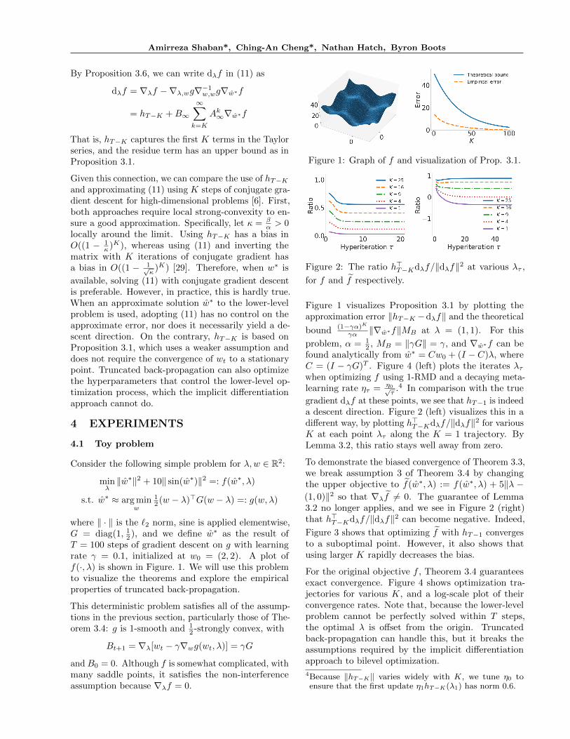
Figure 1: Graph of f and visualization of Prop. 3.1.

Figure 2: The ratio h>T�Kd�f/kd�fk2 at various �⌧ ,

for f and ef respectively.

Figure 1 visualizes Proposition 3.1 by plotting theapproximation error khT�K �d�fk and the theoretical

bound (1��↵)K

�↵ krw⇤fkMB at � = (1, 1). For this

problem, ↵ = 12 , MB = k�Gk = �, and rw⇤f can be

found analytically from w⇤ = Cw0 + (I � C)�, whereC = (I � �G)T . Figure 4 (left) plots the iterates �⌧

when optimizing f using 1-RMD and a decaying meta-learning rate ⌘⌧ = ⌘0p

⌧.4 In comparison with the true

gradient d�f at these points, we see that hT�1 is indeeda descent direction. Figure 2 (left) visualizes this in adi↵erent way, by plotting h>

T�Kd�f/kd�fk2 for variousK at each point �⌧ along the K = 1 trajectory. ByLemma 3.2, this ratio stays well away from zero.

To demonstrate the biased convergence of Theorem 3.3,we break assumption 3 of Theorem 3.4 by changingthe upper objective to ef(w⇤,�) := f(w⇤,�) + 5k� �(1, 0)k2 so that r�

ef 6= 0. The guarantee of Lemma3.2 no longer applies, and we see in Figure 2 (right)that h>

T�Kd�f/kd�fk2 can become negative. Indeed,

Figure 3 shows that optimizing ef with hT�1 convergesto a suboptimal point. However, it also shows thatusing larger K rapidly decreases the bias.

For the original objective f , Theorem 3.4 guaranteesexact convergence. Figure 4 shows optimization tra-jectories for various K, and a log-scale plot of theirconvergence rates. Note that, because the lower-levelproblem cannot be perfectly solved within T steps,the optimal � is o↵set from the origin. Truncatedback-propagation can handle this, but it breaks theassumptions required by the implicit di↵erentiationapproach to bilevel optimization.4Because khT�Kk varies widely with K, we tune ⌘0 toensure that the first update ⌘1hT�K(�1) has norm 0.6.

Truncated Back-propagation for Bilevel Optimization

Figure 3: Biased convergence for ef . The red X marksthe optimal �.

Figure 4: Convergence for f .

4.2 Hyperparameter optimization problems

4.2.1 Data hypercleaning

In this section, we evaluate K-RMD on a hyperparam-eter optimization problem. The goal of data hyper-cleaning [9] is to train a linear classifier for MNIST [30],with the complication that half of our training labelshave been corrupted. To do this with hyperparameteroptimization, let W 2 R10⇥785 be the weights of theclassifier, with the outer objective f measuring thecross-entropy loss on a cleanly labeled validation set.The inner objective is defined as weighted cross-entropytraining loss plus regularization:

g(W,�) =P5000

i=1 ��(�i) log(e>yiWxi) + 0.001kWk2F

where (xi, yi) are the training examples, � denotes thesigmoid function, �i 2 R, and k · kF is the Frobeniusnorm. We optimize � to minimize validation loss, pre-sumably by decreasing the weight of the corruptedexamples. The optimization dimensions are |�| = 5000,|W | = 7850. Franceschi et al. [9] previously solved thisproblem with full RMD, and it happens to satisfy manyof our theoretical assumptions, making it an interestingcase for empirical study.5

We optimize the lower-level problem g through T = 100steps of gradient descent with � = 1 and consider how

5We have reformulated the constrained problem from [9] asan unconstrained one that more closely matches our theo-retical assumptions. For the same reason, we regularizedg to make it strongly convex. Finally, we do not retrainon the hypercleaned training + validation data. This isbecause, for our purposes, comparing the performance ofw⇤ across K is su�cient.

Table 2: Hypercleaning metrics after 1000 hyperiters.

K Test Acc. Val. Acc. Val. Loss F11 87.50 89.32 0.413 0.855 88.05 89.90 0.383 0.8925 88.12 89.94 0.382 0.8950 88.17 90.18 0.381 0.89100 88.33 90.24 0.380 0.88

Figure 5: kd�fk vs. hyperiteration for hypercleaning.

adjusting K changes the performance of K-RMD.6

Our hypothesis is that K-RMD for small K worksalmost as well as full RMD in terms of validation andtest accuracy, while requiring less time and far lessmemory. We also hypothesize thatK-RMD does almostas well as full RMD in identifying which samples werecorrupted [9]. Because our formulation of the problemis unconstrained, the weights �(�i) are never exactlyzero. However, we can calculate an F1 score by settinga threshold on �: if �(�i) < �(�3) ⇡ 0.047, then thehyper-cleaner has marked example i as corrupted.7

Table 2 reports these metrics for variousK. We see that1-RMD is somewhat worse than the others, and thatvalidation loss (the outer objective f) decreases with Kmore quickly than generalization error. The F1 scoreis already maximized at K = 5. These preliminaryresults indicate that in situations with limited memory,K-RMD for small K (e.g. K = 5) may be a reasonablefallback: it achieves results close to full backprop, andit runs about twice as fast.

From a theoretical optimization perspective, we wonderwhether K-RMD converges to a stationary point of f .Data hypercleaning satisfies all of the assumptions ofTheorem 3.4 except that Bt is not full column rank(since M < N). In particular, the validation loss f isdeterministic and satisfies r�f = 0. Figure 5 plots thenorm of the true gradient d�f on a log scale at theK-RMD iterates for various K. We see that, despitesatisfying almost all assumptions, this problem exhibitsbiased convergence. The limit of kd�fk decreases slowlywith K, but recall from Table 2 that practical metricsimprove more quickly.

6See Appendix G.1 for more experimental setup.7F1 scores for other choices of the threshold were verysimilar. See Appendix G.1 for details.

Amirreza Shaban*, Ching-An Cheng*, Nathan Hatch, Byron Boots

4.2.2 Task interaction

We next consider the problem of multitask learning [27].Similar to [9], we formulate this as a hyperparameteroptimization problem as follows. The lower-level objec-tive g(w, {C, ⇢}) learns V di↵erent linear models withparameter set w = {wv}Vv=1:

l(w) +X

1i,jK

Cijkwi � wjk2 + ⇢VX

v=1

kwvk2

where l(w) is the training loss of the multi-class linearlogistic regression model, ⇢ is a regularization constant,and C is a nonnegative, symmetric hyperparametermatrix that encodes the similarity between each pairof tasks. After 100 iterations of gradient descent withlearning rate 0.1, this yields w⇤. The upper-level ob-jective c(w⇤) estimates the linear regression loss of thelearned model w⇤ on a validation set. Presumably, thiswill be improved by tuning C to reflect the true simi-larities between the tasks. The tasks that we considerare image recognition trained on very small subsets ofthe datasets CIFAR-10 and CIFAR-100.8

From an optimization standpoint, we are most inter-ested in the upper-level loss on the validation set, sincethat is what is directly optimized, and its value is agood indication of the performance of the inexact gra-dient. Figure 6 plots this learning curve along withtwo other metrics of theoretical interest: norm of thetrue gradient, and cosine similarity between the trueand approximate gradients. In CIFAR100, the valida-tion error and gradient norm plots show that K-RMDconverges to an approximate stationary point with abias that rapidly decreases as K increases, agreeingwith Proposition 3.1. Also, we find that negative valuesexist in the cosine similarity of 1-RMD, which impliesthat not all the assumptions in Theorem 3.4 hold forthis problem (e.g. Bt might not be full rank, or thethe inner problem might not be locally strong convexaround w⇤.) In CIFAR10, some unusal behavior hap-pens. For K > 1, the truncated gradient and the fullgradient directions eventually become almost the same.We believe this is a very interesting observation butbeyond the scope of the paper to explain.

In Table 3, we report the testing accuracy over 10trials. While in general increasing the number of back-propagation steps improves accuracy, the gaps are small.A thorough investigation of the relationship betweenconvergence and generalization is an interesting openquestion of both theoretical and practical importance.

4.3 Meta-learning: One-shot classification

The aim of this experiment is to evaluate the perfor-mance of truncated back-propagation in multi-task,

8See Appendix G.2 for more details.

Table 3: Test accuracy for task interaction. Few-stepK-RMD achieves similar performance as full RMD.

Method Avg. Acc. Avg. Iter. Sec/iter.

CIFAR-10

1-RMD 61.11± 1.23 3300 0.85-RMD 61.33± 1.08 4950 1.325-RMD 61.31± 1.24 4825 1.4Full RMD 61.28± 1.21 4500 2.2

CIFAR-100

1-RMD 34.37± 0.63 7440 1.05-RMD 34.34± 0.68 8805 1.425-RMD 34.51± 0.69 8660 1.6Full RMD 34.70± 0.64 5670 2.8

0 20000 40000.20

.25

Val Err.1-RMD5-RMD25-RMDFMD

0 20000 40000

10 5

10 3

||d f ||

0 20000 400000.0

0.5

1.0Cosine Sim.

0 10000 20000

2.5

3.0

3.5Val Err.

0 10000 20000

10 3

10 1 ||d f ||

0 10000 200000.0

0.5

1.0Cosine Sim.

Figure 6: Upper-level objective loss (first column), normof the exact gradient (second column), and cosine similarity(last column) vs. hyper-iteration on CIFAR10 (first row)and CIFAR100 (second row) datasets.

stochastic optimization problems. We consider in par-ticular the one-shot classification problem [20], whereeach task T is a k-way classification problem and thegoal is learn a hyperparameter � such that each taskcan be solved with few training samples.

In each hyper-iteration, we sample a task, a training set,and a validation set as follows: First, k classes are ran-domly chosen from a pool of classes to define the sam-pled task T . Then the training set S = {(xi, yi)}ki=1

is created by randomly drawing one training example(xi, yi) from each of the k classes. The validation set Qis constructed similarly, but with more examples fromeach class. The lower-level objective gS(w,�) is

P(xi,yi)2S l(nn(xi;w,�), yi) +

PVj=1 ⇢j ||wj � cj ||2

where l(·, ·) is the k-way cross-entropy loss, andnn(·;w,�) is a deep neural network parametrized byw = {w1, . . . , wV } and optionally hyperparameter �.To prevent overfitting in the lower-level optimization,we regularize each parameter wj to be close to centercj with weight ⇢j > 0. Both cj and ⇢j are hyperpa-rameters, as well as the inner learning rate �. Theupper-level objective is the loss of the trained networkon the sampled validation set Q. In contrast to otherexperiments, this is a stochastic optimization prob-lem. Also, A�(S)(xi) = nn(xi; w⇤,�) depends directlyon the hyperparameter �, in addition to the indirectdependence through w⇤ (i.e. r�f 6= 0).

Truncated Back-propagation for Bilevel Optimization

Table 4: Results for one-shot learning on Omniglotdataset. K-RMD reaches similar performance as fullRMD, is considerably faster, and requires less memory.

Method Accuracy iter. Sec/iter.1-RMD 95.6 5K 0.410-RMD 96.3 5K 0.725-RMD 96.1 5K 1.3Full RMD 95.8 5K 2.2

1-RMD 97.7 15K 0.410-RMD 97.8 15K 0.7Short horizon 96.6 15K 0.1

We use the Omniglot dataset [31] and a similar neuralnetwork as used in [20] with small modifications. Pleaserefer to Appendix G.3 for more details about the modeland the data splits. We set T = 50 and optimize overthe hyperparameter � = {�l1 ,�l2 , c, ⇢, �}. The averageaccuracy of each model is evaluated over 120 randomlysampled training and validation sets from the meta-testing dataset. For comparison, we also try usingfull RMD with a very short horizon T = 1, which iscommon in recent work on few-shot learning [20].

The statistics are shown in Table 4 and the learningcurves in Figure 7. In addition to saving memory, alltruncated methods are faster than full RMD, some-times even five times faster. These results suggest thatrunning few-step back-propagation with more hyper-iterations can be more e�cient than the full RMD. Tosupport this hypothesis, we also ran 1-RMD and 10-RMD for an especially large number of hyper-iterations(15k). Even with this many hyper-iterations, the totalruntime is less than full RMD with 5000 iterations, andthe results are significantly improved. We also find thatwhile using a short horizon (T = 1) is faster, it achievesa lower accuracy at the same number of iterations.

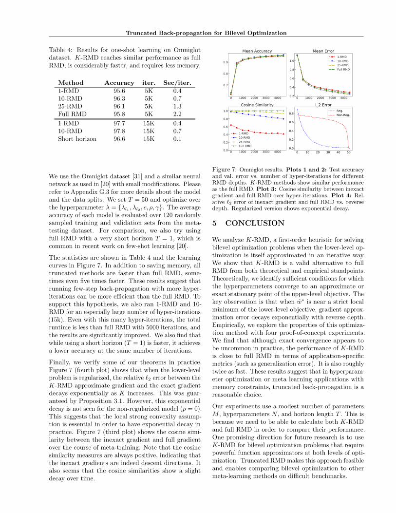
Finally, we verify some of our theorems in practice.Figure 7 (fourth plot) shows that when the lower-levelproblem is regularized, the relative `2 error between theK-RMD approximate gradient and the exact gradientdecays exponentially as K increases. This was guar-anteed by Proposition 3.1. However, this exponentialdecay is not seen for the non-regularized model (⇢ = 0).This suggests that the local strong convexity assump-tion is essential in order to have exponential decay inpractice. Figure 7 (third plot) shows the cosine simi-larity between the inexact gradient and full gradientover the course of meta-training. Note that the cosinesimilarity measures are always positive, indicating thatthe inexact gradients are indeed descent directions. Italso seems that the cosine similarities show a slightdecay over time.

0 1000 2000 3000 4000

0.7

0.8

0.9

Mean Accuracy

0 1000 2000 3000 40000.2

0.4

0.6

0.8

1.0

Mean Error1-RMD10-RMD25-RMDFull RMD

0 1000 2000 3000 40000.0

0.2

0.4

0.6

0.8

1.0Cosine Similarity

1-RMD10-RMD25-RMDFull RMD

0 10 20 30 40 500.0

0.2

0.4

0.6

0.8

l_2 ErrorReg.Non-Reg.

Figure 7: Omniglot results. Plots 1 and 2: Test accuracyand val. error vs. number of hyper-iterations for di↵erentRMD depths. K-RMD methods show similar performanceas the full RMD. Plot 3: Cosine similarity between inexactgradient and full RMD over hyper-iterations. Plot 4: Rel-ative `2 error of inexact gradient and full RMD vs. reversedepth. Regularized version shows exponential decay.

5 CONCLUSION

We analyze K-RMD, a first-order heuristic for solvingbilevel optimization problems when the lower-level op-timization is itself approximated in an iterative way.We show that K-RMD is a valid alternative to fullRMD from both theoretical and empirical standpoints.Theoretically, we identify su�cient conditions for whichthe hyperparameters converge to an approximate orexact stationary point of the upper-level objective. Thekey observation is that when w⇤ is near a strict localminimum of the lower-level objective, gradient approx-imation error decays exponentially with reverse depth.Empirically, we explore the properties of this optimiza-tion method with four proof-of-concept experiments.We find that although exact convergence appears tobe uncommon in practice, the performance of K-RMDis close to full RMD in terms of application-specificmetrics (such as generalization error). It is also roughlytwice as fast. These results suggest that in hyperparam-eter optimization or meta learning applications withmemory constraints, truncated back-propagation is areasonable choice.

Our experiments use a modest number of parametersM , hyperparameters N , and horizon length T . This isbecause we need to be able to calculate both K-RMDand full RMD in order to compare their performance.One promising direction for future research is to useK-RMD for bilevel optimization problems that requirepowerful function approximators at both levels of opti-mization. Truncated RMDmakes this approach feasibleand enables comparing bilevel optimization to othermeta-learning methods on di�cult benchmarks.

Amirreza Shaban*, Ching-An Cheng*, Nathan Hatch, Byron Boots

References

[1] Justin Domke. Generic methods for optimization-based modeling. In Artificial Intelligence andStatistics, pages 318–326, 2012.

[2] Luca Franceschi, Michele Donini, Paolo Frasconi,and Massimiliano Pontil. A bridge between hy-perparameter optimization and larning-to-learn.NIPS 2017 Workshop on Meta-learning, 2017.

[3] James Bergstra and Yoshua Bengio. Randomsearch for hyper-parameter optimization. Journalof Machine Learning Research, 13(Feb):281–305,2012.

[4] Niranjan Srinivas, Andreas Krause, Sham MKakade, and Matthias Seeger. Gaussian processoptimization in the bandit setting: No regret andexperimental design. In Proceedings of the 27thInternational Conference on International Confer-ence on Machine Learning, 2010.

[5] Jasper Snoek, Hugo Larochelle, and Ryan PAdams. Practical bayesian optimization of ma-chine learning algorithms. In Advances in neuralinformation processing systems, pages 2951–2959,2012.

[6] Fabian Pedregosa. Hyperparameter optimizationwith approximate gradient. In International Con-ference on Machine Learning, pages 737–746, 2016.

[7] Stephen Gould, Basura Fernando, Anoop Cherian,Peter Anderson, Rodrigo Santa Cruz, and EdisonGuo. On di↵erentiating parameterized argminand argmax problems with application to bi-leveloptimization. arXiv preprint arXiv:1607.05447,2016.

[8] Dougal Maclaurin, David Duvenaud, and RyanAdams. Gradient-based hyperparameter optimiza-tion through reversible learning. In InternationalConference on Machine Learning, pages 2113–2122,2015.

[9] Luca Franceschi, Michele Donini, Paolo Frasconi,and Massimiliano Pontil. Forward and reversegradient-based hyperparameter optimization. InProceedings of the 34th International Conferenceon International Conference on Machine Learning,2017.

[10] Jelena Luketina, Mathias Berglund, Klaus Gre↵,and Tapani Raiko. Scalable gradient-based tuningof continuous regularization hyperparameters. InInternational Conference on Machine Learning,pages 2952–2960, 2016.

[11] Atilim Gunes Baydin, Robert Cornish, David Mar-tinez Rubio, Mark Schmidt, and Frank Wood. On-line learning rate adaptation with hypergradient

descent. In International Conference on LearningRepresentations, 2018.

[12] Jan Larsen, Lars Kai Hansen, Claus Svarer, andM Ohlsson. Design and regularization of neuralnetworks: the optimal use of a validation set. InNeural Networks for Signal Processing [1996] VI.IEEE Signal Processing Society Workshop, pages62–71. IEEE, 1996.

[13] Yoshua Bengio. Gradient-based optimization ofhyperparameters. Neural computation, 12(8):1889–1900, 2000.

[14] Yunjin Chen, Rene Ranftl, and Thomas Pock.Insights into analysis operator learning: Frompatch-based sparse models to higher order mrfs.IEEE Transactions on Image Processing, 23(3):1060–1072, 2014.

[15] Rich Caruana. Multitask learning. In Learning tolearn, pages 95–133. Springer, 1998.

[16] Rajeev Ranjan, Vishal M Patel, and Rama Chel-lappa. Hyperface: A deep multi-task learningframework for face detection, landmark localiza-tion, pose estimation, and gender recognition.IEEE Transactions on Pattern Analysis and Ma-chine Intelligence, 2017.

[17] Li Fei-Fei, Rob Fergus, and Pietro Perona. One-shot learning of object categories. IEEE transac-tions on pattern analysis and machine intelligence,28(4):594–611, 2006.

[18] Sachin Ravi and Hugo Larochelle. Optimizationas a model for few-shot learning. In InternationalConference on Learning Representations, 2017.

[19] Jake Snell, Kevin Swersky, and Richard S Zemel.Prototypical networks for few-shot learning. In Ad-vances in Neural Information Processing Systems,2017.

[20] Chelsea Finn, Pieter Abbeel, and Sergey Levine.Model-agnostic meta-learning for fast adaptationof deep networks. In International Conference onMachine Learning (ICML), 2017.

[21] Marcin Andrychowicz, Misha Denil, Sergio Gomez,Matthew W Ho↵man, David Pfau, Tom Schaul,and Nando de Freitas. Learning to learn by gra-dient descent by gradient descent. In Advancesin Neural Information Processing Systems, pages3981–3989, 2016.

[22] Ke Li and Jitendra Malik. Learning to optimizeneural nets. arXiv preprint arXiv:1703.00441,2017.

[23] Atilim Gunes Baydin, Barak A Pearlmutter,Alexey Andreyevich Radul, and Je↵rey MarkSiskind. Automatic di↵erentiation in machine

Truncated Back-propagation for Bilevel Optimization

learning: A survey. Journal of Machine LearningResearch, 18:153:1–153:43, 2017.

[24] Laurent Hascoet and Mauricio Araya-Polo. En-abling user-driven checkpointing strategies inreverse-mode automatic di↵erentiation. arXivpreprint cs/0606042, 2006.

[25] Elad Hazan et al. Introduction to online convexoptimization. Foundations and Trends R� in Opti-mization, 2(3-4):157–325, 2016.

[26] Stefan Roth and Michael J Black. Fields of ex-perts: A framework for learning image priors. InIEEE Conference on Computer Vision and Pat-tern Recognition (CVPR), volume 2, pages 860–867. IEEE, 2005.

[27] Theodoros Evgeniou, Charles A Micchelli, andMassimiliano Pontil. Learning multiple tasks withkernel methods. Journal of Machine LearningResearch, 6(Apr):615–637, 2005.

[28] Walter Rudin. Principles of Mathematical Analy-sis, volume 3. New York: McGraw-Hill, 1964.

[29] Jonathan Richard Shewchuk. An introductionto the conjugate gradient method without theagonizing pain, 1994.

[30] Yann LeCun, Leon Bottou, Yoshua Bengio, andPatrick Ha↵ner. Gradient-based learning appliedto document recognition. Proceedings of the IEEE,86(11):2278–2324, 1998.

[31] Brenden M Lake, Ruslan Salakhutdinov, andJoshua B Tenenbaum. Human-level concept learn-ing through probabilistic program induction. Sci-ence, 350(6266):1332–1338, 2015.

[32] Roger A Horn and Charles R Johnson. Matrixanalysis. Cambridge University Press, 1990.

[33] Diederik P Kingma and Jimmy Ba. Adam: Amethod for stochastic optimization. In Interna-tional Conference on Learning Representations,2015.

[34] Kaiming He, Xiangyu Zhang, Shaoqing Ren, andJian Sun. Deep residual learning for image recog-nition. In IEEE Conference on Computer Visionand Pattern Recognition (CVPR), pages 770–778,2016.

[35] Jia Deng, Wei Dong, Richard Socher, Li-Jia Li,Kai Li, and Li Fei-Fei. Imagenet: A large-scalehierarchical image database. In IEEE Confer-ence on Computer Vision and Pattern Recognition(CVPR), pages 248–255. IEEE, 2009.