TRUE MASSES OF RADIAL-VELOCITY EXOPLANETS

TRUE MASSES OF RADIAL-VELOCITY EXOPLANETS

Robert A. BrownSpace Telescope Science Institute, USA; [email protected]

Received 2015 January 12; accepted 2015 April 14; published 2015 MM DD

ABSTRACT

We study the task of estimating the true masses of known radial-velocity (RV) exoplanets by means of directastrometry on coronagraphic images to measure the apparent separation between exoplanet and host star. Initially,we assume perfect knowledge of the RV orbital parameters and that all errors are due to photon statistics. Weconstruct design reference missions for four missions currently under study at NASA: EXO-S and WFIRST-S, withexternal star shades for starlight suppression, EXO-C and WFIRST-C, with internal coronagraphs. These DRMsreveal extreme scheduling constraints due to the combination of solar and anti-solar pointing restrictions,photometric and obscurational completeness, image blurring due to orbital motion, and the “nodal effect,” which isthe independence of apparent separation and inclination when the planet crosses the plane of the sky through thehost star. Next, we address the issue of nonzero uncertainties in RV orbital parameters by investigating their impacton the observations of 21 single-planet systems. Except for two—GJ 676 A b and 16 Cyg B b, which areobservable only by the star-shade missions—we find that current uncertainties in orbital parameters generallyprevent accurate, unbiased estimation of true planetary mass. For the coronagraphs, WFIRST-C and EXO-C, themost likely number of good estimators of true mass is currently zero. For the star shades, EXO-S and WFIRST-S,the most likely numbers of good estimators are three and four, respectively, including GJ 676 A b and 16 Cyg B b.We expect that uncertain orbital elements currently undermine all potential programs of direct imaging andspectroscopy of RV exoplanets.

Key words: methods: statistical – planetary systems – planets and satellites: detection – techniques: radial velocities

1. INTRODUCTION

To date, hundreds of exoplanets have been discovered by theradial-velocity (RV) technique. Not only have these objectschanged the course of the history of astronomy and opened richnew fields of study, the known RV planets are special objectsof further research, mainly because they are relatively nearbyand because they revolve around bright, well-known stars.Without doubt, scientists will one day know each of these RVplanets intimately as individual objects, each with uniqueorigins, attributes, and environments, just like the solar-systemplanets today. We can now look ahead to the next steps towardthat goal, which are to determine the true masses m( )p ofknown RV planets and to obtain simple diagnostic spectra oftheir atmospheres. To support those ends, this paper presents ananalytic framework for mass determination by direct astro-metry. We use that framework to estimate the performance offour space optical systems currently under study. Thesemissions—which proponents say could be implemented inthe 2020s—are WFIRST-C, a 2.4 m telescope with an internalcoronagraph (Spergel et al. 2015), EXO-S, a 1.1 m telescopewith a star shade (Seager et al. 2015), EXOC, a 1.4 m telescopewith an internal coronagraph (Stapelfeldt et al. 2015),WFIRST-S, a 2.4 m telescope with an external star shade(Seager et al. 2015; Chapter 8).

Two types of research motivate the science requirement fordetermining mp. The first type investigates the formation andevolution of planetary systems. Just as explaining thedistributions of planetary mass and orbital distance has longbeen a focus of solar-system studies, today such research hasbeen taken to the next level, addressing those distributionsbroadly—ultimately, everywhere in the universe. The secondtype of research investigates planetary atmospheres, where theplanetary mass enters into the scale height. Knowing the scaleheight is important for interpreting planetary spectra, which is

relevant because we plan follow-on spectroscopy as an adjunctto the mass-determination program.In the current work, which is a point calculation, we define

the science requirement on mass determination to be

σ≡ =F

m0.10 (1)

pmp

mp

where Fmp is the fractional uncertainty of the estimate of mp,and σmp is the standard deviation of mp. The WFIRST-C andEXO-C study reports use Fmp = 0.10, and EXO-S andWFIRST-S use Fmp = 0.20.In the case of spectroscopy, we are guided by the treatment

of Maire et al. (2012), which discusses the spectroscopicopportunities for SPICES, a notional 1.5 m telescope with thepurpose of atmospheric characterization of cold exoplanets. Forgiant planets, they identify methane bands at 620, 730, and790 nm, in order of increasing strength. Shallower water bandsare located at 720 and 820 nm. Longer wavelengths aredisadvantageous due to reduced spatial resolution and, in thecase of CCD detectors, falling sensitivity due to silicontransparency. We therefore adopt I band as the nominal rangefor RV planet imaging and spectroscopy, and 760 nm as thenominal wavelength for calculations. Maire et al. found that a“spectral resolution of at least 50 is required to identify themain bands of the spectra of giant planets as well as super-Earths.” We have chosen = 70spc and a nominal targetsignal-to-noise ratio (S/N) of 10 in the continuum forspectroscopyOur observing plan envisions starting the spectroscopic

exposure immediately after directly imaging a possible RVplanet. The reason for acting quickly is that the source mayshortly disappear behind the central field stop or otherwisebecome unobservable. (From Tables 3–6, we expect most

The Astrophysical Journal, 00:000000 (28pp), 2015 Month Day© 2015. The American Astronomical Society. All rights reserved.

APP Template V1.01 Article id: apj513330 Typesetter: MPS Date received by MPS: 19/05/2015 PE: CE : LE:

UNCORRECTED PROOF

1

mailto:[email protected]

detections to occur near the inner working angle (IWA), whichis the nominal radius of the field stop.)

In the case of true-mass determination, our framework issomewhat complicated, but also new and interesting. Even withperfect knowledge of the RV orbits—which we assume untilSection 7—successfully planning the observations is achallenging task. When we introduce errors into the RV orbitalparameters, we find that estimating mp with any acceptableaccuracy becomes impossible except for a few exoplanetsat most.

To the best of our knowledge, no science requirements onthe accuracy of estimating mp have yet been proposed in print,nor have any measurement requirements been derived from anysuch requirements, nor has the performance of any candidatemission so far been tested taking into account all key factors.This paper provides the needed framework, which includesmeasurement requirements. We find those requirements dependstrongly on the orbital phase of the planet, especially near nodecrossings as well as solar-avoidance restrictions, variableobscuration near the central field stop, the systematic limit tothe depth of search exposures, variation of local zodi withecliptic latitude and longitude, observational overheads, and theblurring of images due to the orbital motion of the planet.

Traub et al. (2014) uses a simplified model to calculate howmany RV planets could be detected in how many days ofexposure time by various coronagraph designs for WFIRST-C.The Traub et al. results are not relevant to this report becausethey do not treat true-mass estimation.

After developing our framework for estimating mp by directastrometry on coronagraphic images, we calculate analyticdesign reference missions (DRMs) for the four missions understudy. These DRMs assume perfect knowledge of the RVorbital parameters for each exoplanet. In Section 7, we relaxthis assumption and investigate the effect of current uncertain-ties in orbital parameters. The effect is devastating, and it callsfor an urgent program to improve the accuracy of RV orbitalparameters, at least for the exoplanets identified as offeringvalue for true-mass determination.

As is well known, RV observations estimate the projectedmass of an exoplanet, mp sin i, where i is the usually unknowninclination of the planetary orbit. In this paper, we treat theprojected mass as a single variable—“msini”—which is an RVorbital parameter. Today, we know msini for hundreds of RVplanets, but we know mp only for a few: the transitingexoplanets, for which sin i ≈ 1, and mp is trivial to compute.For non-transiting RV planets, we must make some newmeasurement to constrain i and thereby remove the “sin idegeneracy” in planetary mass. Here, there are at least twopossibilities. Brown (2009) presents a way to estimate i fromthe “photometric orbit” of reflected starlight from non-transiting, Kepler-type exoplanets with RV orbital solutions.The host stars of these exoplanets are generally located at sogreat a distance that direct imaging will be out of the questionfor the foreseeable future.

Dumusque (2014) describes a method for fitting stellaractivity to estimate the stellar inclination, which is the same asthe orbital inclination of a planet if the orbital and stellar polesare aligned. The application of this technique to long-periodRV exoplanets—such as the input catalog of this study—hasnot been developed.

In this paper, we present a complementary approach forestimating i to get mp. This approach, which is applicable to

nearby RV planets, estimates i from the apparent separation s,between the planet and the host star, where s is measured bydirect astrometry on a coronagraphic image. In this case, wewill show that a single measurement of s is, in principle,sufficient to estimate i.We are not aware of any other way to measure mp and take a

follow-on spectrum. Nevertheless, various statisticalapproaches have been offered for estimating the true distribu-tion of a quantity “projected” by a factor sin i, includingrotation rates of unresolved stars (Chandrasekhar &Münch 1950), microlensing (Giannini & Lunine 2013;Brown 2014), and RV planets (Jorisson et al. 2001; Zucker& Mazeh 2001; Marcy et al. 2005; Udry & Santos 2007;Brown 2011; Ho & Turner 2011; Lopez & Jenkins 2012).Nevertheless, Brown (2011) shows that a usefully constraineddistribution of the unprojected quantity may demand a sampleof thousands or tens of thousands of projected values; certainlymore than the mere hundreds we have in the case of currentlyknown RV planets.To outline the sections ahead, in Section 2, we derive our

method of estimating the value of S/N required to estimate mp

with fractional accuracy Fmp. In Section 3, we assemble a miseen place of DRM basics: in Section 3.1, we document thebaseline parameters and assumptions for the four missionsunder study; in Section 3.2, we describe our input catalog ofpotentially observable RV planets; and, in Section 3.3, wedescribe our exposure-time calculator. In Section 4, we define acube of intermediate information, which realizes a mission andgenerates diagnostic reports. In Section 5, we introduce theconcept of the “analytic” DRM, including scheduling algo-rithm, merit function, union completeness (UC), and medianexposure times. In Section 6, we compare the baselineperformance of four missions sharing the goal of determiningmp for known RV planets. Section 7 investigates the negativeimpact on estimating mp due to the current levels of uncertaintyin RV orbital parameters. Section 8 summarizes and calls forintensive RV observations to improve the accuracy of RVorbital solutions adequately to support a robust program oftrue-mass estimation by direct astrometry with high-contrastimagery.

2. ANALYTIC FRAMEWORK OF TRUE-MASSESTIMATION

In this section, we deconstruct the center term in Equation (1)with the goal of determining the values of S/N it demands, as afunction of fractional uncertainty Fmp, the Julian day of theastrometric observation (t), and the RV orbital parameters,which are assumed at this point to be errorless. In Section 2.1,as a start, we find the required astrometric uncertainty (σs),which varies with the orbital phase of the planet. In Section 2.2,we describe the “roll convolution” protocol (Section 2.2.1) andderive an empirical calibration of σs as a function S/N(Section 2.2.2). Finally, Equation (18) gives the desiredfunctional form of S/N.In this paper, we variously employ 11 non-independent

orbital parameters, which fall into five groups: intrinsic,orientational, orbital phase, planetary, and stellar. Semimajoraxis (a) and eccentricity (e) are intrinsic to the true orbitalellipse in space. The planet’s argument of periapsis (ωp) andthe inclination (i) are Euler rotations that define the orientationof the RV orbit. The period (P) and the Julian day of anyperiapsis (t0), determine the orbital phase in terms of the mean

2

The Astrophysical Journal, 00:000000 (28pp), 2015 Month Day Brown

Original Text

and

anomaly (M). The amplitude of the RV signal is proportional tothe projected planetary mass (msini). The stellar parameters arethe mass of the host star (ms), which connects P and a, thestar’s constant or offset RV (V) and its first derivative (V̇ ),which are needed to fit RV data sets, as we illustrate inSection 7.

We ignore and set to zero the longitude of the ascendingnode (Ω), which defines the position angle of the orbit on thesky. It has no bearing on our subject.

Catalogs of RV exoplanets typically provide ωs, which is theargument of periapsis of the star, from which we can computeω ω= + °180p s for the planet.

When fitting an RV data set, we solve for seven RVparameters: a, e, M0, ωp, msini, V, V̇}, where M0 is the meananomaly at the time of the first RV data point. We adopt thecatalog value of the stellar mass ms and compute P and t0 asneeded from a, M0, and ms. The following section treats i, thecrucial parameter not known from RV that is needed toestimate mp from msini.

In the first part of this paper, Sections 2–6, we assume thatthe orbital parameters of each RV planet are known withouterror. In Section 7, we address the issue of nonzerouncertainties in orbital parameters and show that they arereally important.

2.1. Required Astrometric Uncertainty, σs

We introduce a Cartesian coordinate system with the star atthe origin, +x toward north, +y toward east, and +z toward theobserver. We use the same (x, y, z) coordinate systemthroughout.

We introduce the “base a-e orbit,” which is not the true orbit,not the apparent orbit, but a well-defined theoretical orbit. Thebase a–e orbit is related to the true orbit by three Euler rotationsabout the star. The base a–e orbit lies on the plane of the skythrough the star, oriented with its semimajor axis on the x axisand its periapsis on the +x axis. The concept of the base a–eorbit is useful for separating the physical parameters of the trueorbit (a, e)—where the science is—from the rotations thatproduce the apparent orbit ( Wω i, ,p ), but are not physicalproperties of the planetary system.

The theoretical position of the planet before the orbit isrotated is described by the parametric equations:

ν νν ν

===

x r

y r

z

( )cos( )sin

0, (2)

0

0

0

where the planet-star distance is

νν

=−

+( )

ra e

e( )

1

1 cos, (3)

2

with r and a in arcseconds, where ν is the true anomaly, whichis the root of the equation

ν = +−

e

e

Etan

2

1

1tan

2, (4)

in which the eccentric anomaly (E) is the root of Keplerʼsequation,

− =E e E Msin , (5)

in which the mean anomaly or orbital phase is:

=−

⎜ ⎟⎛⎝

⎞⎠M π

t t

P2 , (6)0

where t is the current time and both t and t0 are measuredin days.The position of the planet in space, (x, y, z), is found by first

rotating the vector (x0, y0, z0) by ωp around the +z axis, andthen rotating it by i around the –x axis:

ω ω

ω ω

ω ω

= −

= +

= − +

( )( )

x x y

y x y i

z x y i

cos sin

sin cos cos

sin cos sin . (7)

p p

p p

p p

0 0

0 0

0 0

Here, z is unobservable, being along the line of sight. Theapparent position of the planet on the sky is (x, y). The apparentseparation in arcseconds between star and planet is

ω ω

ω ω=

−

+ +

( )( )

sx y

x y i

cos sin

sin cos cos. (8)

P P

P P

0 02

0 02 2

If we were analyzing an actual image of an RV planet, wewould estimate mp by dividing the value of msini by the valueof sin i inferred from the planetary image. The actual measuredquantity in such an image is the apparent separation s—not i orsin i itself. To obtain sin i from s, we invert Equation (8):

ω ω=

+ −

+i

x y s

x ysin

sin cos. (9)

P p

02

02 2

0 0

We see from Equations (2), (3), (8), and (9) that only a limitedrange of s is possible for any RV planet at any time, that is,

⩽ ⩽s s smin max, where

ω ω= −s x ycos sin (10)P Pmin 0 0

and

= +s x y , (11)max 02

02

which is the true, physical separation in space. Here, alldistances are rendered in arcseconds.From Equations (8) and (10), we see that smin occurs when

=i π 2, which is the edge-on orientation of the orbit. FromEquations (9), (11), smax occurs when i = 0, which is the face-on orientation, for which ≡z 0.To determine σs, the astrometric uncertainty in s, we must

approach the foregoing information from a different direction,starting with sin i, for which we know the distribution but notthe value. The uncertainty goal for isin —which is σ isin —isdetermined by the science requirement in Equation (1).Therefore, from Equation (9), in the linear approximation,

σ σ

σω ω

= ∂∂

=+ + −

=+ −

−i

s

x y x y s

s

x y s

s F

sin

sin cos

1, (12)

s i

ip p

sin

1

sin0 0 0

202 2

02

02 2

mp

3


Original Text

system).

Original Text

=0,

where we have used the fact that Fsini=Fmp because we haveassumed the orbital parameter msini is without error—an issuewe revisit in Section 7.

It is apparent from Equation (12) that σs goes to zero as s

goes to +x y02

02 , which occurs at a node, when the planet

crosses the plane of the sky through the host star. At a node, thesensitivity of s to i vanishes, and therefore it temporarilybecomes impossible to estimate i from a measurement of s, nomatter how precise.

2.2. Required Signal-to-Noise Ratio

Two further analyses are required to determine the value ofS/N required by Equation (1) to achieve the desired true-massaccuracy. In Section 2.2.1, we derive the relationship betweenS/N and detector counts’signal counts and noise counts —

for the roll-deconvolution protocol we adopt for this study. InSection 2.2.2, we empirically determine the relationshipbetween astrometric error σs and S/N. Later, in Section 3.3,we will show how to compute the exposure time (τ) to achievethe desired S/N. At that point, we will have a three-step bridgefrom Equation (1) by which we can compute τ for any RVplanet, on any mission day, for any assumed inclination i.

2.2.1. Roll Deconvolution: S/N, , and “Roll deconvolution” is a scheme to reduce the effect of

speckles, which—assuming the optics are stable—do not movewhen the telescope is rolled around the optic axis by an angle ϕin the time between the two otherwise equal exposures (e.g.,Müller and Weigelt 1987). Assume (x, y) coordinates that arefixed on the focal-plane detector, with origin (0, 0) located onthe optic axis of the telescope at the position of the host star.Assume the two exposures produce two data arrays—images I1and I2—each with half the total exposure time, τ. The positionin I2 of a point located at position (x1, y1) in I1 is:

ϕ ϕ ϕ ϕ= − +( )x y x y x y( , ) cos sin , sin cos . (13)2 2 1 1 1 1

Data analysis for the roll-convolution protocol involves thefollowing steps.

Step 1. Subtract I2 from I1, creating the difference image I3.The purpose of this step is to remove the speckles, which theroll has not moved, leaving only speckle noise.

If we hypothesize that a planet is located at (x1, y1) in I1, weexpect to find the value + 2 signal photons to be collected inthe optimal virtual photometric aperture (VPA) of Ψ =− 131

Nyquist-sampling pixels centered at (x1, y1) in I3 (Bur-rows 2003; Burrows et al. 2006).

If the VPA is centered at (x2, y2) in I3, we expect to find thevalue − 2. In the field of I3, well away from (x1, y1) and (x2,y2), we expect to find noise of zero mean and standarddeviation √ , because we expect 2 noise photons to becollected in the field for each of I1 and I2.

Step 2. Perform the reverse rotation on I3, creating image I4.Step 3. Subtract image I4 from I3, creating the final image, I

5. We now find signal photons in the VPA centered at (x1, y1)in I5. (We ignore the two negative, ghost images on eitherside.) In the field, the standard deviation of the noise in theVPA is now 2 . Therefore, the S/N for roll deconvolution is

=

+S N

2. (14)

In Section 3, we discuss the calculation of the exposure time τneeded to achieve a goal value of S/N.

2.2.2. Empirical Determination of S/N Required by σs

A single roll-deconvolved image (e.g., I5) of a known RVplanet yields estimates of three quantities: (1) the brightness ofthe planet relative to the star (expressed in stellar magnitudes asΔmag) and (2 and 3) the planet’s two-dimensional position,(x, y), also relative to the star. With the origin of coordinatespositioned on the star, the apparent separation of the planet is

≡ +s x y2 2 . In this section, we use Monte Carlo experi-ments to estimate σs, the standard deviation or uncertainty in s,as a function of S/N—or equivalently S/N as a function of σs, asneeded. These experiments use least-squares fits to estimate theposition and brightness of the planet in noisy, simulatedimages, which serve as analogs to the roll-deconvolved imagesexpected in the missions.In these experiments, we use two control parameters, S/N

and the count ratio:

≡cr , (15)

which are equivalent to and as control parameters becauseof Equation (14).The Monte Carlo experiments to determine the relationship

between σs, S/N, and cr involve nine steps, as follows. We (1)define a 15-by-15 detector array of critically sampling pixelswith width λ ′D2 radians, where D′ is the diameter of the exitpupil. We desire to populate the pixels with signal counts inproportion to the point-spread function (PSF) randomlysituated on the detector. To this end, we (2) generate a pixel-integrated PSF (piPSF) centered on (x, y) = (0, 0), and then,using Whittaker–Shannon interpolation, we translate piPSF to arandom location (xtrue, ytrue) on the detector in the range− < <x y4 , 4true true pixels.

Next, we introduce photons. For deliberate choices of thecontrol parameters, S/N and cr, we (3) compute and using Equations (14) and (15), (4) multiply piPSF by , and(5) replace each pixel’s resulting value of piPSF × by anumber drawn from a Poisson random value divided byvpae = 0.85, which is the efficiency of the VPA—i.e., the sumof piPSF over the 13 pixels. This correction ensures that, onaverage, photons will be collected in the VPA, as intended.To account for background noise, we (6) add to each pixel in

the detector a value drawn from the random deviate for theSkellam distribution, both parameters of which have been setequal to 13, which is the mean value of background noisecounts per pixel. The result emulates the noise in the differenceof two noisy images.Next, to estimate the astrometric error in the estimated

position of the planet, we (7) perform a least-squares fit toestimate the values of , —which yields S/N—and (xfit,yfit). Our fitting routine is the FINDMINIMUM function inMATHEMATICA, which uses the Levenberg–Marquardtalgorithm. The starting point of the fit is the position of themaximum value in the data array. We (8) estimate theastrometric error as the distance of (xfit, yfit) from (xtrue, ytrue):

≡ − + −s x x y y( ) ( ) . (16)error fit true2

fit true2

For the Monte Carlo experiment, we (9) perform steps 1–810,000 times for each value of S/N, with fresh realizations of

4


Original Text

i

Original Text

)=(0,

Original Text

deviate with a mean equal to that

Original Text

vpae=0.85,

the noise and the true image location each trial, and from theresults, estimate σs as the rms value of serror.

The Monte Carlo trials produce two immediate findings.First, we find that the results of this experiment are independentof cr in the range 10−1–10−4, and we therefore adopt the singlevalue cr = 10−2 for ongoing computations.

Second, in 10,000 Monte Carlo trials for various choices ofS/N < 8, we find that a fraction of the peak values will be noisefluctuations remote from and unrelated to the planet. Thisfraction increases as S/N decreases and the probabilityincreases that the least-squares fit will not find the planetaryimage but will stall on a local minimum of pure noise. Whenthat happens, the result is an outlier value of serror. We want tounderstand these outliers—and hopefully minimize or preventthem, because in real data they might be indistinguishable froma faint planetary signal.

We document the outlier issue in Figure 1, as follows. Foreach of 18 values of S/N in the range 2–100, we produce10,000 values of serror by steps 1–8 above. If we knew the valueof σs—which we do not, and in fact we are trying to determineit—we would expect (serror/σs)

2 to be distributed as χ2with

two degrees of freedom. For S/N < 8, however, a considerablefraction of Monte Carlo trials produce outliers with lowprobabilities of being random noise. To identify and removedthe outliers, we apply the principle that the estimatedoccurrence probability of a value X or greater for the variablex is 1 − CDFx(X), where CDFx the cumulative distributionfunction of x. In the current case, X ≡ (serror/σs)

2, and we applythe inverse of the stated rule to learn the cutoff. That is, wewant to learn the value of (serror/σs)

2 such that the probability ofthe distribution producing that value or greater randomly is10−4, which is a reasonable threshold for this project, where ourMonte Carlo sample size is typically 104. We learn the cutoffvalue CO by solving the equation 10−4 = 1 − CDFχ2[2](CO)for CO, where CDFχ2[2] is the CDF of the χ2

distribution withtwo degrees of freedom. The solution is CO = 18.4207.

With the desired value of CO in hand, we return to the 18sets of 10,000 values of serror, one set for each of the 18 valuesof S/N under study. For each set, our next task is to find thevalue of σs that produces—after outliers have been removed—the best match between the empirical distribution of (serror/σs)

2

and the theoretical χ2distribution with two degrees of freedom.

We use the statistic of the Kolmogorov–Smirnov (KS) test to

measure the closeness of the match (Press et al. 2007, Section14.3.3). The KS test compares a theoretical distribution—inthis case the χ2

distribution with two degrees of freedom—withan empirical distribution—in this case the sample of values of(serror/σs)

2 after the outliers have been removed. The best valueof σs minimizes the KS test statistic. The results are shown inFigures 1 and 2.When planning exposure times, we adopt the floor value

⩾S N 8 to avoid outliers. As a result of this floor,observations with a S/N = 8 will have astrometric uncertaintiesσs smaller than called for by Equation (12).

For σΔ > 8s , where Δ is the width of a Nyquist pixel inarcsec:

λΔ =′ × −D2 4.848 10

, (17)6

the requirement is

σ= Δ = Δ

+ −s

x y s FS N

1(18)

s 02

02 2

mp

and for σΔ ⩽ 8s , we have

=S N 8. (19)

In Section 3.3, we describe the process of estimating theexposure time τ needed to achieve the required accuracy in theplanetary mass. The calibration in Figure 2 and Equations (18)and (19) play essential roles in that process. For each RVexoplanet, each in its own unique way according to its orbitalparameters and orbital phase, the desired mass uncertaintybegets a maximum value of the astrometric uncertainty σs,which begets the minimum value of S/N, which begets therequired exposure time, τ—the value of which also depend ondesign parameters, the Julian day, and any value of theinclination i.

3. MISE EN PLACE

In Section 3.1, we summarize the design parameters thatdefine our “baseline” performance estimates of science out-comes. In Section 3.2, we describe our input catalog of knownRV planets. In Section 3.3, we discuss the calculation of

Figure 1. Fraction of outliers vs. S/N in 10,000 Monte Carlo trials at eachpoint. Red line: adopted minimum value S/N = 8, which is the cutoff to avoidoutliers.

Figure 2. Astrometric uncertainty σs in Nyquist pixels as a function of S/N.Each point is the result of a least-squares fit to minimize the Kolmogorov–Smirnov test statistic computed for a data set of 10,000 values of serror withoutliers removed. Black line: the function (S/N)−1. Red line: minimum value S/N = 8, which is the cutoff to avoid outliers.

5


Original Text

=1

exposure time τ. In Section 4, we introduce the cube ofintermediate information that realizes a mission. In Section 5,we introduce the concept of an analytic DRM. In Section 6, weshow DRM results for the four missions under study.

3.1. Baseline Parameters and Assumptions

Table 1 documents the baseline assumptions and parametersfor the four missions under study here, and indicates whetherwe regard them as instrumental (defining the observingsystem), astronomical (defining the sky), or science-opera-tional parameters (indicating how we would expect to use theobservatory to investigate known RV planets).

On 2015 April 7, NASA released study reports on EXO-C,EXO-S, andWFIRST-C (Seager et al. 2015; Spergel et al. 2015;Stapelfeldt et al. 2015). Our choices of instrumental parametersare broadly consistent with the values in those reports.Reasonable variations in the baseline parameters could notqualitatively change our top-level conclusions in Section 8.

As in Brown (2015), and consistent with Maire et al. (2012),we adopt the operational wavelength λ = 760 nm (I band), andresolving powers = 5 (imaging) and = 70 (spectro-scopy). These choices reflect our view of the priority of thediagnostic features of methane and molecular oxygen thatoccur in the range 700–820 nm. The spectroscopic resolvingpower of 70 is reasonably matched to the expected widths ofthose features (Des Marais et al. 2002, Maire et al. 2012).

The diameter of the exit pupil, D′, which contributes to theend-to-end efficiency and governs the size of the planetaryimage, is less than D for EXO-C due to the Lyot mask. EXO-Sand WFIRST-S have no Lyot mask, so D′ = D. Even thoughWFIRST-C includes a Lyot mask, the correct choice is D′ = Dfor that mission also, due to the cancelling effects of the innerand outer radii of the exit pupil. That is, the large inner radiusof the Lyot mask in WFIRST-C removes low spatialfrequencies in favor of high frequencies which tends to reduceimage size, while the smaller outer radius, D′ <D, tends toincrease it. As a result, in John Krist’s optical modeling, thecentral portion of the PSF for WFIRST-C does not differ bymore than a few percent from that of an idealized 2.4 mtelescope with D′ = D. Therefore, we use D′ = D = 2.4 m forWFIRST-C to ensure the correct size of a Nyquist pixel, Δ andVPA. We introduce a “Lyot mask correction” (LMC = 0.08) toensure we include Lyot mask losses—but only for the case ofWFIRST-C.

We assume that the pixel width Δ critically samples theplanetary image on the detector according to the Nyquistcriterion, i.e., Δ = λ/2D′.

For EXO-S and EXO-C, we assume a CCD detector withdark noise υ = 0.00055, read noise σ = 2.8, read-out cadencetr = 2000 s, and quantum efficiency ò = 0.8. For WFIRST, weassume a photon-counting detector with υ = 0, σ = 0, andò = 0.8, which is an idealization.

We assume sufficiently stable optics to support speckledisambiguation and noise reduction by roll deconvolution, asdescribed in Section 2.2.1.

Scattered starlight is suppressed to a level specified by ζ,which is defined as the ratio of the intensity of scatteredstarlight in the detection zone to the central intensity of thetheoretical Airy image of the star.

3.2. Input Catalog

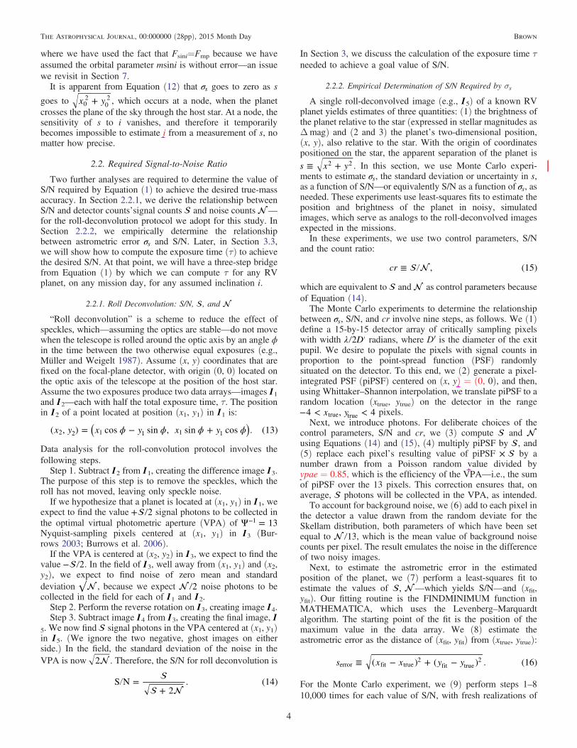
Our input catalog of known RV planets for each mission wasselected from the list at www.exoplanets.org using the criterionthat the raw angular separation ≡s araw (1 + e)/d > IWA,where a is the semimajor axis, e is the orbital eccentricity, andd is the stellar distance. sraw is the maximum possible apparentseparation for a planet with parameters a, e, and d. It does nottake into account the orientation of the orbit, particularly ωp,the argument of periapsis of the planet. If =e 0, ωp generallyreduces the maximum achievable separation (smax) to a smallervalue, smax < sraw.Figure 3 shows the stars in input catalogs and the restrictions

of the adopted values of sraw for WFIRST-C, WFIRST-S, EXO–C, and EXO–S.Table 2 shows the union input catalog of RV planets and

host stars, including a working selection of data items for eachexoplanet.

3.3. Exposure Time, τ

The exposure time τ described here is for planning andscheduling observations, only. During the observation, weassume that observers will follow images and spectradeveloping in real time, as photons accumulate in the detectors.The actual S/N will be determined on the fly, by the observer’sdecision to stop or continue an exposure.For a host star of I magnitude Istar, we seek the exposure time

τ necessary to achieve the desired value of S/N on ahypothetical planet of magnitude Iplanet=Istar + Δmag, whereΔmag is the flux ratio of planet to star expressed in stellarmagnitudes:

θΔ = − Φ+

⎛⎝⎜⎜

⎞⎠⎟⎟p

R

x ymag 2.5 log ( ) , (20)

o

2

02 2

where p is the geometric albedo of the planet, Φ is the phasefunction, θ is the phase angle, which is the planetocentric anglebetween observer and star:

θω ω

≡− +

+

( )i x y

x yarccos

sin sin cos. (21)

p p0 0

02

02

and R is the assumed planetary radius in arcseconds.Section 2.10 in Brown (2015) states and explains our basic

algorithm for computing τ, with two exceptions.The first exception is that we use D′ (exit aperture) instead of

D (entrance aperture) in Equation (15) of Brown (2015), forreasons explained in the third paragraph of Section 3.1 of thispaper.The second exception—a change to the exposure-time

algorithm—is that we upgrade the algorithm to allow for atapered central obscuration. The focal planes of these opticalsystems are complicated, and we simply adopt the followingequations.The IWA is still the nominal radius of the central field

obscuration, but the end-to-end efficiency (h) is not, however,expected to be a step function at apparent separation s = IWA.Due to the finite size of the image—FWHM λ= ′ −D h isbetter described as a function of s. For sufficiently largeseparations, >s s1, then =h h0, as in earlier treatments, where

≡ h LMC reflTrans, (22)0

6


http://www.exoplanets.org

Original Text

And

Original Text

=760 nm

Original Text

′=

Original Text

′=

Original Text

(LMC=0.08)

Original Text

Δ=

Original Text

=0.00055,

Original Text

=2.8,

Original Text

=2000 s,

Original Text

=0.8.

Original Text

=0,

Original Text

=0,

Original Text

=0.8,

Table 1Baseline Parameters

# Parameter Symbol Value Units Comment Type

1 wavelength λ 760 nm L science operational2 spectral resolving power imaging img 5 L L science operational

3 spectral resolving powerspectroscopy

spc 70 L L science operational

4 entrance aperture D 1.1 EXO-S, 1.4 EXO-C, 2.4 WFIRST-C, -S m L instrumental5 exit aperture D′ 1.1 EXO-S, 0.85 EXO-C, 2.4 WFIRST-C, -S m L Instrumental6 pixel width Δ 0.071 EXO-S, 0.092 EXO-C, 0.033 WFIRST-C, -S arcsec Nyquist : λ D2 ′ dependent parameter7 dark noise υ 0.00055 EXO-S, 0.00055 EXO-C, 0. WFIRST-C, -S L L instrumental8 read noise σ 2.8 EXO-S, 2.8 EXO-C, 0. WFIRST-C, -S L L instrumental9 readout cadence tr 2000 EXO-S, 2000 EXO-C, N/A WFIRST-C − S, s L science operational10 inner working angle IWA 0.100 EXO-S, 0.224 EXO-C, 0.196 WFIRST-C, 0.100

WFIRST-Sarcsec L instrumental

11 scattered starlight ζ 5 × 10–10 EXO-S, 10–9 EXO-C, 10–9 WFIRST-C, 10–10

WFIRST-SAiry intensity of stellar image

centerL instrumental

12 Lyot mask correction LMC 1.0 EXO-S, 1.0 EXO-C, 0.08 WFIRST-C, 1.0 WFIRST-S L corrects Lyot mask throughput instrumental13 detector QE ò 0.8 L L instrumental14 refl/trans efficiency reflTra-

ns0.45 EXO-S, 0.4 EXO-C, 0.25 WFIRST-C, -S L L instrumental

15 planet–radius R 1 RJupter L astronomical16 geometric albedo p 0.5 L L astronomical17 phase function Φ Lambertian L L astronomical18 mission start t 2 460 310.5 JD 1/1/2024 science operational19 solar avoidance γ1 30° EXO-S 45° EXO-C 54° WFIRST-C 40° WFIRST-S degree L instrumental20 antisolar avoidance γ2 83° EXO-S 180° EXO-C 126° WFIRST-C 83° WFIRST-S degree L instrumental21 setup time tsetup 8 EXO-S 0.5 EXO-C 0.5 WFIRST-C 8 WFIRST-S days per observation science operational22 mission duration tmission 1826 days L science operational23 zodiacal light Z 7 zodis 23rd magnitude arcsec−2 astronomical24 limiting delta magnitude Δmag0 22.5 magnitudes L science operational25 S/N, imaging S/Nimg 8 L science operational26 S/N, spectroscopy S/Nspc 10 L science operational27 mass accuracy σmp/mp 0.10 L science operational28 sharpness Ψ 0.08 L instrumental29 zero-magnitude flux F0 4885 photons cm−2 nm−1 s−1 I band, 760 nm science operational

Note. For the coronagraphs, IWA = 3 λ/D forWFIRST-C and IWA = 2 λ / D for EXO-C. Z = 7 zodis consists of 1 zodi of local zodi and 6 zodis of exozodi. The mission duration is somewhat arbitrary, but long enoughto accommodate optimized visits to all the observable exoplanets for each optical system. The limiting delta magnitude (Δmag) is the systematic limit or “noise floor,” as determined by the stability of the optical system(Brown 2005). IWA, the inner working angle, is the nominal radius of the central field obscuration. The value of IWA for WFIRST-C and the values for setup time and reflective/transmissive efficiency for all missionswere recommended by Stuart Shaklan.

7

TheAstro

physica

lJourn

al,

00:000000(28pp),

2015Month

Day

Brow

n

Original Text

IWA=3

Original Text

IWA=2

where the LMC is the Lyot mask correction introduced inSection 3.1, ϵ is the detector quantum efficiency, and reflTransis the product of the reflective or transmissive efficiencies of allthe optical elements in series. For sufficiently small separations,s < s0, h = 0. Therefore, our model for the dependence of h on sis:

≡h h s( ), (23)0

where is a piecewise continuous function.For internal coronagraphs, we assume h = 0.5 at s = IWA,

where the PSF is centered on the edge of the obscuration. Theexact value of h at s = IWA depends of the design ofcoronagraph. At smaller angles, s < IWA, internally scatteredstarlight ζ increases and efficiency h decreases—both sorapidly that we assume (s < IWA)=0 for coronagraphs. Sofar, tolerancing studies for internal coronagraphs have treatedonly the range s > IWA (Shaklan et al. 2011a). Following theliterature, then, our taper function for coronagraphs is

= <

= + − ⩽ < +

= ⩾ +

⎜ ⎟⎛⎝

⎞⎠

s s IWA

s IWA

FWHMIWA s IWA FWHM

s IWA FWHM

( ) 0 for ,

0.5 1 for ,

1.0 for .

(24)

A star shade has a solid inner disk surrounded by taperedpetals. Here, we define IWA to be the angular subtense of theradius of the disk plus the length of the petals, and we use thevalue IWA = 100 mas for both EXO-S and WFIRST-S.

While some star-shade studies have considered performancefor s < IWA (Shaklan et al. 2010, 2011b; Glassman et al. 2010),we focus in this paper on the EXO-S and WFIRST-Simplementations under study at NASA, which have beentoleranced assuming planets are not detectable if s < IWA.Therefore, we assume a step function for in the case of star

shades:

= <= ⩾

s s IWAs IWA

( ) 0 for , and1.0 for . (25)

For starshades the shape of the petals, not the telescope PSF,determines the throughput around the s= IWA.

4. CUBE OF INTERMEDIATE INFORMATION

The preceding sections prepare us to populate a “cube ofintermediate information,” which is a data structure. Deriva-tives from the cube—we call them “reports”—help constructDRMs, which estimate mission performance and provideinsights into the true nature of the challenges involved withcharacterizing RV planets.Our cube has three dimensions: absolute time (t in Julian

day), RV planet identifier (HIP or other catalog name), andinclination angle i. Time t runs from mission start to missionstop, for a total of 1826 days for the assumed five yearsmissions. Potentially observable RV planets number 16 or 55,for coronagraphs or star shades, respectively, as explained inSection 3.2. The number of random values of i is 4000 in thecurrent study, generated by the appropriate random deviate,

−− cos (11 ), where is a uniform random deviate on therange 0–1. Multiplying the three cardinalities, we see that thecube has 117 million or 402 million cells or addresses, forcoronagraphs or star shades, respectively.The information in each cell of the cube is a vector with at

least eight elements (but possibly more for convenience): (S/N,s, Δmag , τ), plus four flags: fpointing, fSVP&O, fspatial, andftemporal. For each cell address (t, HIP, i), and using theparameters in Table 1 that are appropriate to each mission, wecompute the orbital solution as described in Section 2.1,compute S/N as described in Equations (18) and (19), take sfrom the orbital solution, compute Δmag from Equations (20)and (21), and compute τ as described in Section 3.3.The four flags are binary variables. A “one” means that the

flag criterion is satisfied—for that planet, on that day, for that

Figure 3. Distance (d) and value of raw separation a (1 + e) for the 436 known RV planets in the data base at www.exoplanets.org on 2014 March 1. The curves parsethe planets into two groups, those to the right, which are totally obscured and therefore never observable, and those to the left, which may be observable at some timeduring the mission, depending on the orbital inclination, i, and argument of periapsis, ω .p

8


www.exoplanets.org

Original Text

=0.5

Original Text

< IWA)=0

Original Text

IWA=100

Table 2Union Input Catalogs of RV Planets and Host Stars

CoronagraphsStar

ShadesPlanetName HIP V

B– V I d (pc)

Mass(Solar)

R.A.(hr)

Decl.(°)

EclipticLongitude

(°)

EclipticLatitude

(°)Raw Separa-tion (arcsec) a (AU)

Period(days) e ω Star (°)

Time of Peri-apsis (JD)

msin i

1 L ✓ GJ 317 b L 12 1.52 9.63 9.1743 0.24 8.7 −23.5 140.8 −40.1 0.124 0.95 692.9 0.19 344 2451639 1.182 L ✓ HD

7449 b5806 7.5 0.58 6.88 38.521 1.05 1.2 −5.0 15.2 −12.0 0.1105 2.34 1275 0.82 339 2455298 1.31

3 ✓ ✓ upsilonAnd d

7513 4.1 0.54 3.51 13.492 1.31 1.6 41.4 38.6 29.0 0.2372 2.52 1278 0.27 270 2453937 4.12

4 L ✓ HD10180 h

7599 7.33 0.63 6.65 39.017 1.06 1.6 −60.5 340.4 −61.6 0.101 3.42 2248 0.15 184 2453619 0.21

5 L ✓ HD10647 b

7978 5.52 0.55 4.92 17.434 1.1 1.7 −53.7 350.8 −57.3 0.1345 2.02 1003 0.16 336 2450960 0.93

6 L ✓ HD13931 b

10626 7.61 0.64 6.92 44.228 1.02 2.3 43.8 47.3 28.2 0.1188 5.15 4218 0.02 290 2454494 1.88

7 ✓ ✓ epsilonEri b

16537 3.72 0.88 2.79 3.2161 0.82 3.5 −9.5 48.2 −27.7 1.312 3.38 2500 0.25 6 2448940 1.05

8 L ✓ HD24040 b

17960 7.5 0.65 6.8 46.598 1.18 3.8 17.5 59.2 −2.6 0.1099 4.92 3668 0.04 154 2454308 4.02

9 L ✓ HD30562 b

22336 5.77 0.63 5.09 26.42 1.28 4.8 −5.7 69.8 −27.9 0.1559 2.34 1157 0.76 81 2450131 1.33

10 ✓ ✓ GJ 179 b 22627 11.96 1.6 9.15 12.288 0.36 4.9 6.5 72.4 −15.9 0.2376 2.41 2288 0.21 153 2455140 0.8211 L ✓ HD

33636 b24205 7 0.59 6.36 28.369 1.02 5.2 4.4 77.3 −18.5 0.1704 3.27 2128 0.48 340 2451205 9.27

12 ✓ ✓ HD39091 b

26394 5.65 0.6 5 18.315 1.07 5.6 −80.5 273.9 −76.0 0.2998 3.35 2151 0.64 330 2447820 10.09

13 L ✓ HD38529 c

27253 5.95 0.77 5.13 39.277 1.34 5.8 1.2 86.4 −22.2 0.1242 3.6 2146 0.36 17.9 2452255 12.26

14 L ✓ 7 CMa b 31592 3.95 1.06 2.83 19.751 1.34 6.6 −19.3 101.7 −42.3 0.104 1.8 763 0.14 12 2455520 2.4315 L ✓ HD

50499 b32970 7.21 0.61 6.55 46.126 1.28 6.9 −33.9 109.8 −56.5 0.1052 3.87 2458 0.25 259 2451220 1.74

16 L ✓ HD50554 b

33212 6.84 0.58 6.21 29.913 1.03 6.9 24.2 102.5 1.4 0.1091 2.26 1224 0.44 7.4 2450646 4.40

17 L ✓ betaGem b

37826 1.15 1 0.1 10.358 2.08 7.8 28.0 113.2 6.7 0.1731 1.76 589.6 0.02 355 2447739 2.76

18 L ✓ HD70642 b

40952 7.17 0.69 6.43 28.066 1 8.4 −39.7 144.2 −56.7 0.1172 3.18 2068 0.03 205 2451350 1.91

19 L ✓ HD72659 b

42030 7.46 0.61 6.8 49.826 1.07 8.6 −1.6 131.4 −19.6 0.1164 4.75 3658 0.22 261 2455351 3.17

20 ✓ ✓ 55 Cnc d 43587 5.96 0.87 5.04 12.341 0.91 8.9 28.3 127.7 10.4 0.4525 5.47 4909 0.02 254 2453490 3.5421 L ✓ GJ 328 b 43790 9.98 1.32 8.41 19.8 0.69 8.9 1.5 135.8 −15.2 0.3068 4.43 4100 0.37 290 2454500 2.3022 L ✓ HD

79498 b45406 8.02 0.71 7.26 46.104 1.06 9.3 23.4 134.1 7.1 0.108 3.13 1966 0.59 221 2453210 1.35

23 ✓ ✓ HD87883 b

49699 7.57 0.96 6.56 18.205 0.8 10.1 34.2 141.7 21.3 0.3006 3.58 2754 0.53 291 2451139 1.76

24 L ✓ HD89307 b

50473 7.02 0.59 6.38 32.363 0.99 10.3 12.6 151.9 1.9 0.1211 3.27 2166 0.20 4.9 2452346 1.79

25 ✓ ✓ 47UMa c

53721 5.03 0.62 4.36 14.063 1.06 11.0 40.4 149.1 31.1 0.2789 3.57 2391 0.10 295 2452441 2.55

26 L ✓ 47UMa b

″ ″ ″ ″ ″ ″ ″ ″ ″ ″ 0.1542 2.1 1078 0.03 334 2451917 0.55

27 L ✓ HD106252 b

59610 7.41 0.64 6.73 37.707 1.01 12.2 10.0 179.1 10.5 0.1026 2.61 1531 0.48 293 2453397 6.96

28 L ✓ HD117207 b

65808 7.26 0.72 6.49 33.047 1.03 13.5 −35.6 214.4 −24.3 0.1294 3.74 2597 0.14 73 2450630 1.82

29 L ✓ HD128311 c

71395 7.48 0.97 6.46 16.502 0.83 14.6 9.7 213.2 23.7 0.1301 1.75 923.8 0.23 28 2456987 3.25

30 ✓ ✓ HD134987 c

74500 6.47 0.69 5.73 26.206 1.05 15.2 −25.3 232.8 −7.1 0.249 5.83 5000 0.12 195 2451100 0.80

31 L ✓ kappaCrB b

77655 4.79 1 3.74 30.497 1.58 15.9 35.7 222.7 53.9 0.1002 2.72 1300 0.13 83.1 2453899 1.97

32 L ✓ HD142022 b

79242 7.7 0.79 6.86 34.329 0.9 16.2 −84.2 264.5 −61.3 0.1307 2.93 1928 0.53 170 2450941 4.47

9

TheAstro

physica

lJourn

al,

00:000000(28pp),

2015Month

Day

Brow

n

Original Text

e

Table 2(Continued)

CoronagraphsStar

ShadesPlanetName HIP V

B– V I d (pc)

Mass(Solar)

R.A.(hr)

Decl.(°)

EclipticLongitude

(°)

EclipticLatitude

(°)Raw Separa-tion (arcsec) a (AU)

Period(days) e ω Star (°)

Time of Peri-apsis (JD)

msin i

33 ✓ ✓ 14 Her b 79248 6.61 0.88 5.68 17.572 1.07 16.2 43.8 223.2 62.9 0.2286 2.93 1773 0.37 22.6 2451372 5.2134 L ✓ HD

147513 b80337 5.37 0.63 4.7 12.778 1.07 16.4 −39.2 250.7 −17.3 0.1291 1.31 528.4 0.26 282 2451123 1.18

35 L ✓ GJ 649 b 83043 9.7165 1.52 7.34 10.345 0.54 17.0 25.7 248.9 48.1 0.1422 1.13 598.3 0.30 352 2452876 0.3336 ✓ ✓ HD

154345 b83389 6.76 0.73 5.98 18.587 0.89 17.0 47.1 241.7 69.1 0.2367 4.21 3342 0.04 68.2 2452831 0.96

37 L ✓ GJ676 Ab

85647 9.585 1.44 7.68 16.45 0.71 17.5 −51.6 264.8 −28.3 0.1463 1.82 1057 0.33 85.7 2455411 4.90

38 ✓ ✓ mu Ara c 86796 5.12 0.69 4.38 15.511 1.15 17.7 −51.8 267.2 −28.4 0.3782 5.34 4206 0.10 57.6 2452955 1.7539 L ✓ mu Ara b ″ ″ ″ ″ ″ ″ ″ ″ ″ ″ 0.1111 1.53 643.3 0.13 22 2452365 1.8940 L ✓ HD

169830 c90485 5.9 0.52 5.33 36.603 1.41 18.5 −29.8 276.1 −6.5 0.1309 3.6 2102 0.33 252 2452516 4.06

41 L ✓ HD181433 d

95467 8.38 1.01 7.32 26.759 0.78 19.4 −66.5 281.6 −43.9 0.1671 3.02 2172 0.48 330 2452154 0.54

42 L ✓ 16 CygB b

96901 6.25 0.66 5.54 21.213 0.96 19.7 50.5 321.2 69.5 0.1316 1.66 798.5 0.68 85.8 2446549 1.64

43 L ✓ HD187123 c

97336 7.83 0.66 7.12 48.263 1.04 19.8 34.4 309.5 54.3 0.1253 4.83 3806 0.25 243 2453580 1.94

44 ✓ ✓ HD190360 b

98767 5.73 0.75 4.93 15.858 0.98 20.1 29.9 312.6 48.9 0.329 3.97 2915 0.31 12.9 2453541 1.54

45 L ✓ HD192310 c

99825 5.73 0.88 4.8 8.9111 0.8 20.3 −27.0 300.0 −7.0 0.1753 1.18 525.8 0.32 110 2455311 0.07

46 L ✓ HD196885 b

101966 6.39 0.51 5.83 33.523 1.23 20.7 11.2 315.8 28.6 0.1122 2.54 1333 0.48 78 2452554 2.94

47 L ✓ HD204313 d

106006 8.006 0.7 7.26 47.483 1.02 21.5 −21.7 317.5 −6.5 0.1063 3.94 2832 0.28 247 2446376 1.61

48 L ✓ HD204941 b

106353 8.45 0.88 7.52 26.954 0.74 21.5 −21.0 318.7 −6.0 0.1298 2.55 1733 0.37 228 2456015 0.27

49 ✓ ✓ GJ 832 b 106440 8.66 1.52 6.29 4.9537 0.45 21.6 −49.0 308.6 −32.5 0.7694 3.4 3416 0.12 304 2451211 0.6450 ✓ ✓ GJ 849 b 109388 10.42 1.52 8.05 9.0959 0.49 22.2 −4.6 332.7 6.3 0.2691 2.35 1882 0.04 355 2451488 0.8351 L ✓ HD

216437 b113137 6.04 0.66 5.33 26.745 1.12 22.9 −70.1 305.3 −55.5 0.1226 2.49 1353 0.32 67.7 2450605 2.17

52 ✓ ✓ HD217107 c

113421 6.17 0.74 5.38 19.857 1.11 23.0 −2.4 344.9 3.9 0.4076 5.33 4270 0.52 199 2451106 2.62

53 L ✓ HD220773 b

115697 7.06 0.66 6.35 50.891 1.16 23.4 8.6 355.8 11.3 0.1467 4.94 3725 0.51 259 2453866 1.45

54 L ✓ HD222155 b

116616 7.12 0.64 6.43 49.1 1.13 23.6 49.0 20.4 45.8 0.1214 5.14 3999 0.16 137 2456319 2.03

55 L ✓ gammaCep b

116727 3.21 1.03 2.13 14.102 1.26 23.7 77.6 60.1 64.7 0.1572 1.98 905.6 0.12 49.6 2453121 1.52

Note. Check marks indicate whether the planet is possibly observable. I magnitudes were generated from V and B–V using Neill Reid’s photometric data, as described in Section 2.6 of Brown (2015).

10

TheAstro

physica

lJourn

al,

00:000000(28pp),

2015Month

Day

Brow

n

value of i—and a “zero” means that at least one flag criterion isviolated. fpointing refers to solar and anti-solar avoidance (γ1, γ2),which is described in detail in Section 2.8 of Brown (2015).fSVP&O is the “single-visit photometric and obscurational”(SVP&O) flag (Brown 2004, Brown 2005). =f 1SVP&O if

>s IWA and Δmag < Δmag0, where Δmag0 is the limitingdelta magnitude, which is the systematic limit or “noise floor,”as determined by the stability of the optical system(Brown 2005, 2015). fspatial pertains to image smearing; thisflag is zero for a planet that would move more than FWHM =λ/D′ during the exposure time, but otherwise one. ftemporal

pertains to the continuity of an exposure; it is zero if fpointing = 0on any day during a multi-day search exposure, or if theexposure time would extend beyond the end of the mission.Otherwise, fpointing = 1.

The cube fully realizes a mission because it contains everyimportant piece of information for constructing a DRM with agranularity of one mission day. We use the cube to produce twotypes of report: completeness reports and median reports. Thepremier application of both types of report is to constructDRMs, as we demonstrate in Sections 5 and 6.

5. DESIGN REFERENCE MISSIONS

DRMs are mission simulations inside a computer. Thegeneral goals of an analytic DRM are (1) to comparealternative mission concepts on a fair, objective basis, (2) tosupport the optimization of mission parameters, and (3) tocommunicate realistic expectations for a mission’s productivityand scientific outcomes, should it be implemented.

A DRM is defined by a variety of instrumental, astronom-ical, and science-operational parameters, listed with baselinevalues in Table 1. In the current implementation, the cube ofintermediate information described in Section 4 is the linkbetween Table 1 and the DRM. That is, as described inSections 5.1–5.3, we draw completeness reports and medianreports from the cube to construct DRMs. The missionparameters and algorithms are fully embodied by the cube.

In Section 6, we describe baseline DRMs for the fourmissions under study.

5.1. Scheduling Algorithm and Merit Function, At the heart of a DRM is the scheduling algorithm, with the

duty of selecting the next observation after the current exposureis terminated, on any day in the mission. As a rule, thescheduling algorithm selects the observation with the highestcurrent value of the merit function (). Obviously, musthave a lot of “moving parts” to account for all the factorsinvolved. Nevertheless, the complexity of becomes morestructured and convenient because of the cube. The goal of thissection is to deconstruct into completeness reports andmedian reports from the cube.

—or “discovery rate” or “benefit-to-cost ratio”—is theprobability of a detecting an RV planet divided by estimatedtotal time cost of the observation, which is the estimatedexposure time τ plus the setup time tsetup:

τ

≡+UC

t. (26)

setup

In the case of a single search observation—as envisioned herefor each RV planet in a DRM—the probability of observationalsuccess is the UC (Brown 2005, 2015, Brown & Soummer

2010). Success itself—discovering the RV planet in the direct-search observation, yes or no—is a Bernoulli random variablewith probability UC. In search programs with revisits, theprobability is UC with a Bayesian correction (Brown &Soummer 2010; Brown 2015).It is useful to keep in mind that random variables—notably i

and observational success given UC—are involved in buildingDRMs. This means that the DRMs are themselves randomvariables, often calling for estimation by Monte Carloexperiments.Section 5.2 describes how we estimate the numerator in

Equation (26)—UC—from the cube by means of a complete-ness report. Section 5.3 describes how we estimate the searchexposure time τ from the cube as a median report. Section 5.3also describes how we estimate the exposure time τspec, forpossible follow-on spectroscopy.

5.2. Union Completeness

As explained in Section 4, we carry four flags at each cubeaddress (t, HIP, i): fpointing, fSVP&O, fspatial, and ftemporal. Eachflag indicates whether or not a detection criterion is satisfied atthat location in the cube. Each cube address identifies apotential observation in the DRM. A potential observation is“invalid”—infeasible or doomed to failure—if any of the fourflags is zero, and the observation is “valid” if the flags are allequal to one. For any selected planet, HIP, on any selectedmission day, t, UC is estimated by the fraction of the 4000random values of i that result in valid cube addresses.The same procedure works separately for each of the four

components of UC. That is, we can estimate each constituentcompleteness—pointing permission, SVP&O, spatial, or tem-poral—by the sum of the associated flag divided by the numberof trials, which is 4000 here. (UC may not, however, be theproduct of the four constituent completenesses because theflags may not be independent.)See Figures 4 and 6 for two illustrative completeness panels,

in this case for mu Ara b observed by EXO-S and for 14 Her bobserved by WFIRST-C.

5.3. Median Exposure Times, τ̃ and τ̃spec

At the time the scheduling algorithm is selecting the nextsearch observation, the actual value of i is not known, andtherefore the correct exposure time is unknowable in advance.Nevertheless, for each planet and mission day, the cube carries4000 random values of i, each with an associated value of τ.Therefore, we estimate τ as the median of the values of τ invalid observations (τ̃).Note that the median exposure time τ̃ is for planning and

scheduling observations, only. During the observation, obser-vers will follow images and spectra developing in real time, asphotons accumulate in the detectors. The actual S/N will bedetermined on the fly, by the observer’s decision to stop orcontinue an exposure.τ̃ is an example of a median report. By the same principles,

we can produce median reports for the other cell contents—S/N, s, and Δmag, as well as functions of medians, notably inthe cases of merit function and the exposure time for follow-on spectroscopy. These we can estimate by the function appliedto the medians—if we can establish that the function commuteswith the median function, which we can do in the case of the

11


Original Text

FWHM

Original Text

=0

Original Text

=1.

exposure time calculator and therefore in the denominator ofEquation (26).

See Figures 5 and 7 for two illustrative median panels, formu Ara b observed by EXO-S and for 14 Her b observed byWFIRST-C.

6. BASELINE DRMS FOR THE FOUR MISSIONS

The following tables and plots, Tables 3–6 and Figures 8–11,document our four baseline DRMs for the four missions understudy. Each DRM uses the baseline parameters listed for the

mission in Table 1. For each observation of a planet, thescheduling algorithm has chosen the day of the missionmaximum value of the merit function .It is important to keep in mind that the exposure time τ

described here is for the planning and scheduling ofobservations, only. During an observation, observers willfollow images and spectra developing in real time, as photonsaccumulate in the detectors. The actual S/N will be determinedon the fly, by the observer’s decision to stop or continue anexposure.

Figure 4. Completeness panel for mu Ara b observed by EXO-S. Compare with the median panel in Figure 5. Plot 1A shows the doubled windowing due to both solarand antisolar avoidance for EXO-S. Plot 1B shows orbital period of mu Ara b, 643 days. Plots 1C and 1D show only the first set of node crossings; the second set isabsent because those node crossings occur when <s IWA, which means that τ is invalid due to fSVP&O = 0. (See the discussion in the penultimate paragraph ofSection 4.) In Plot 1D, we see that temporal completeness is modulated by a factor not present in spatial completeness: pointing permission, which varies periodicallyin absolute time (i.e., the abscissa), with a period of the Earth’s orbital period of 365 days. In Plot 1E, we see that the four-flag UC is sparse and spikey, and thatopportunities to launch a search observation with a high probability of success are only four at most.

12


It is also important to note that each exposure time has beencalculated with the mass measurement in mind, such that thegoal Fmp = 0.10 is included in UC, τ, and therefore in andftemporal, and utimately in each line of each DRM. The signatureof Fmp can be traced from Equation (1) to σs in Equation (12),to S/N in Equation (18), to τ in Equation (15) in Section 2.10of Brown (2015), to ftemporal and into three of the eightelements in the cells of the cube of intermediate information, oninto UC, and thus by multiple avenues into the lines ofeach DRM.

For the star-shade missions, EXO-S and WFIRST-S, tsetup is16-times larger than the 0.5 days for setting upcoronagraph missions. Therefore, in most cases, the medianexposure time in column 12 is much smaller than the setuptime, tsetup. In the limit of ignoring τ̃ with respect to tsetup,Equation (26) says that prioritizing observations by UC is thesame as prioritizing by .No attempt has been made to identify scheduling conflicts,

which are only a minor issue at worst, because the schedulesare already dilute and become more dilute when the least

Figure 5. Typical median values vs. mission day, here for mu Ara b observed by EXO-S. Compare with the completeness panel Figure 4. Dashed lines in Plots 2A and2B: IWA and Δmag0, which reveal that the regions of value zero in Plot 1B are due to obscuration (s < IWA), not to insufficient planet brightness, Δmag > Δmag0.Plot 2D shows that all valid days (i.e., the four flags are all ones) have S/N requirements elevated above the default S/N = 8, due to their proximity to nodes. In Plot2E, for merit function , notice that the best times to observe mu Ara b (maximum ) are limited to a few days around 0, 650, and 1350 mission day, where ∼ 0.1.In Section 6, Table 5, line 5, we see that, in developing the DRM, the scheduling algorithm chose to observe mu Ara b on 645 mission day.

13


Original Text

=0.10

Table 3Tabular DRM for WFIRST-S

Planet Name MedianApparent

MedianFlux

Median S/N Mission Day UnionCompleteness UC

Cumulative UC ObservingTime (days)

CumulativeObserving

MeritFunction

MedianSearch

MedianSpectroscopic

Separation s RatioΔmag

Time (days) (1/days) ExposureTime

ExposureTime (days)

1 beta Gem b 0.137 21.2 8.0 476 1.000 1.00 8.000 8.0 0.125 0.00 0.002 epsilon Eri b 0.577 19.9 8.0 818 1.000 2.00 8.000 16.0 0.125 0.00 0.003 gamma Cep b 0.118 19.4 8.0 512 0.999 3.00 8.000 24.0 0.125 0.00 0.004 HD 192310 c 0.132 18.6 8.0 60 0.999 4.00 8.000 32.0 0.125 0.00 0.005 47 UMa c 0.152 20.2 8.0 1719 0.999 5.00 8.001 40.0 0.125 0.00 0.026 upsilon And d 0.139 19.6 10.8 149 0.998 5.99 8.000 48.0 0.125 0.00 0.017 47 UMa b 0.114 19.3 8.0 1253 0.998 6.99 8.000 56.0 0.125 0.00 0.018 HD 190360 b 0.218 21.1 8.0 1066 0.997 7.99 8.011 64.0 0.124 0.01 0.169 GJ 832 b 0.342 20.0 8.0 797 0.998 8.99 8.017 72.0 0.124 0.02 0.2410 HD 10647 b 0.107 19.6 9.3 391 0.996 9.98 8.002 80.0 0.124 0.00 0.0211 mu Ara b 0.103 19.2 20.0 748 0.996 10.98 8.003 88.0 0.124 0.00 0.0412 mu Ara c 0.282 21.5 8.0 16 0.996 11.98 8.009 96.0 0.124 0.01 0.1213 7 CMa b 0.101 19.8 57.3 180 0.996 12.97 8.008 104.1 0.124 0.01 0.1114 HD 154345 b 0.147 20.8 8.0 1350 0.996 13.97 8.039 112.1 0.124 0.04 0.5515 GJ 649 b 0.108 18.4 8.1 1365 0.992 14.96 8.008 120.1 0.124 0.01 0.1116 14 Her b 0.174 20.7 8.0 1032 0.994 15.95 8.021 128.1 0.124 0.02 0.2917 HD 147513 b 0.104 20.4 13.6 1753 0.989 16.94 8.008 136.1 0.123 0.01 0.1218 HD 128311 c 0.110 19.5 8.0 1796 0.987 17.93 8.011 144.1 0.123 0.01 0.1519 HD 217107 c 0.206 21.3 8.0 1 0.989 18.92 8.036 152.2 0.123 0.04 0.5020 HD 134987 c 0.161 21.4 8.0 1088 0.983 19.90 8.072 160.2 0.122 0.07 1.0121 GJ 849 b 0.173 19.4 8.0 334 0.987 20.89 8.141 168.4 0.121 0.14 1.9722 GJ 676 A b 0.107 19.4 8.0 1733 0.969 21.86 8.074 176.5 0.120 0.07 1.0323 HD 87883 b 0.120 19.9 12.7 1633 0.962 22.82 8.059 184.5 0.119 0.06 0.8224 HD 216437 b 0.101 20.4 38.7 1490 0.973 23.79 8.180 192.7 0.119 0.18 2.5225 HD 38529 c 0.115 21.5 17.8 1688 0.954 24.74 8.155 200.9 0.117 0.16 2.1726 HD 39091 b 0.197 21.1 36.5 40 0.926 25.67 8.282 209.1 0.112 0.28 3.9527 HD 70642 b 0.102 20.5 21.7 1375 0.926 26.59 8.390 217.5 0.110 0.39 5.4628 HD 50554 b 0.102 20.7 30.1 843 0.916 27.51 8.669 226.2 0.106 0.67 9.3629 HD 117207 b 0.108 21.0 8.9 1675 0.838 28.35 8.167 234.4 0.103 0.17 2.3430 HD 142022 b 0.115 21.2 16.0 1003 0.939 29.29 9.542 243.9 0.098 1.54 21.5931 GJ 179 b 0.140 19.8 8.0 214 0.944 30.23 9.919 253.8 0.095 1.92 26.8632 HD 169830 c 0.105 22.2 30.2 1158 0.858 31.09 10.361 264.2 0.083 2.36 33.0533 HD 33636 b 0.139 21.3 31.7 958 0.744 31.83 10.726 274.9 0.069 2.73 38.1734 HD 13931 b 0.107 21.6 16.5 1653 0.729 32.56 11.598 286.5 0.063 3.60 50.3735 HD 181433 d 0.119 20.8 23.7 69 0.675 33.24 11.434 297.9 0.059 3.43 48.0736 GJ 317 b 0.107 20.0 9.7 1328 0.908 34.14 17.619 315.6 0.052 9.52 133.2437 HD 30562 b 0.128 20.9 8.0 798 0.385 34.53 8.011 323.6 0.048 0.01 0.1538 16 Cyg B b 0.116 20.2 9.7 1799 0.251 34.78 8.010 331.6 0.031 0.01 0.1439 HD 89307 b 0.116 22.0 44.7 1611 0.623 35.40 29.573 361.2 0.021 21.57 302.0240 HD 204941 b 0.114 22.0 16.5 1543 0.592 35.99 32.766 393.9 0.018 24.77 346.7241 HD 222155 b 0.108 21.8 13.4 1618 0.159 36.15 9.527 403.4 0.017 1.53 21.3842 HD 196885 b 0.105 21.0 26.4 828 0.109 36.26 8.460 411.9 0.013 0.46 6.4443 HD 7449 b 0.104 22.4 24.4 742 0.432 36.70 43.382 455.3 0.010 35.38 495.3544 55 Cnc d 0.442 22.5 72.0 1725 0.028 36.72 20.054 475.3 0.001 12.05 168.7645 kappa CrB b 0.100 20.9 867.3 731 0.000 36.72 26.825 502.2 0.000 18.82 263.55

14

TheAstro

physica

lJourn

al,

00:000000(28pp),

2015Month

Day

Brow

n

Table 3(Continued)


MedianFlux



CumulativeObserving

MeritFunction

MedianSearch

MedianSpectroscopic



ExposureTime (days)

46 HD 24040 b L L L L L L L L L L L47 HD 72659 b L L L L L L L L L L L48 GJ 328 b L L L L L L L L L L L49 HD 204313 d L L L L L L L L L L L50 HD 79498 b L L L L L L L L L L L51 HD 220773 b L L L L L L L L L L L52 HD 50499 b L L L L L L L L L L L53 HD 10180 h L L L L L L L L L L L54 HD 187123 c L L L L L L L L L L L55 HD 106252 b L L L L L L L L L L L

Note. UC is the probability of a successful detection. The scheduling algorithm chooses the mission day of maximize . Cumulative UC is the expectation value of the total number of planets recovered, to that point.The numbers labeling the points in Figure 8 refer to line numbers in this table. The red points in Figure 8 offer a 90% or better probability of successfully achieving the mass accuracy in Equation (1). Ellipses indicatethat a planet is not observable at all, assuming the parameters in Table 1.

15

TheAstro

physica

lJourn

al,

00:000000(28pp),

2015Month

Day

Brow

n

Table 4Tabular DRM for EXO-S


MedianFlux



CumulativeObserving

MeritFunction

MedianSearch

MedianSpectroscopic



ExposureTime (days)

1 beta Gem b 0.137 21.2 10.4 476 1.000 1.00 8.000 8.0 0.125 0.00 0.012 epsilon Eri b 0.560 19.9 8.0 812 1.000 2.00 8.001 16.0 0.125 0.00 0.013 gamma Cep b 0.117 19.4 8.0 512 0.999 3.00 8.000 24.0 0.125 0.00 0.004 upsilon And d 0.126 19.4 13.9 128 0.995 3.99 8.003 32.0 0.124 0.00 0.055 47 UMa b 0.113 19.3 9.8 1253 0.995 4.99 8.004 40.0 0.124 0.00 0.086 HD 192310 c 0.127 18.6 8.0 49 0.995 5.98 8.002 48.0 0.124 0.00 0.047 47 UMa c 0.143 20.1 8.0 1701 0.994 6.98 8.009 56.0 0.124 0.01 0.228 HD 10647 b 0.106 19.6 19.7 391 0.987 7.96 8.053 64.1 0.123 0.05 1.279 HD 190360 b 0.197 21.0 8.0 1124 0.987 8.95 8.100 72.2 0.122 0.10 2.6010 mu Ara b 0.103 19.2 42.1 748 0.982 9.93 8.062 80.2 0.122 0.06 1.3711 mu Ara c 0.277 21.4 8.0 1 0.985 10.92 8.090 88.3 0.122 0.09 2.3012 GJ 832 b 0.346 19.9 8.0 1041 0.993 11.91 8.179 96.5 0.121 0.18 4.7413 7 CMa b 0.101 19.8 120.8 180 0.982 12.89 8.142 104.6 0.121 0.14 2.6714 14 Her b 0.169 20.7 8.0 1043 0.962 13.85 8.223 112.9 0.117 0.22 5.8915 HD 147513 b 0.104 20.4 28.6 1753 0.966 14.82 8.339 121.2 0.116 0.34 8.4916 HD 154345 b 0.143 20.8 8.0 1350 0.975 15.80 8.461 129.7 0.115 0.46 12.2717 GJ 649 b 0.107 18.4 16.8 1365 0.962 16.76 8.351 138.0 0.115 0.35 9.1918 HD 217107 c 0.203 21.3 8.0 1 0.936 17.69 8.416 146.4 0.111 0.42 11.0119 HD 128311 c 0.107 19.5 14.4 1803 0.916 18.61 8.339 154.8 0.110 0.34 8.8920 HD 134987 c 0.158 21.4 8.0 1087 0.897 19.51 8.856 163.6 0.101 0.86 22.8321 GJ 849 b 0.168 19.4 8.0 334 0.925 20.43 9.720 173.4 0.095 1.72 46.4322 HD 87883 b 0.110 19.7 19.3 1650 0.801 21.23 9.139 182.5 0.088 1.14 30.1723 GJ 676 A b 0.105 19.4 15.6 1733 0.846 22.08 11.316 193.8 0.075 3.32 89.1624 HD 216437 b 0.101 20.4 76.4 1490 0.827 22.91 15.057 208.9 0.055 7.06 182.7525 HD 38529 c 0.113 21.4 31.9 1693 0.678 23.58 13.433 222.3 0.050 5.43 142.9826 HD 117207 b 0.106 20.9 16.4 1675 0.677 24.26 14.632 236.9 0.046 6.63 178.2827 HD 30562 b 0.128 20.9 11.5 798 0.352 24.61 8.241 245.2 0.043 0.24 6.2628 16 Cyg B b 0.115 20.1 21.9 1067 0.222 24.83 8.506 253.7 0.026 0.51 13.1029 HD 39091 b 0.197 21.1 66.7 38 0.446 25.28 18.094 271.8 0.025 10.09 262.7130 HD 70642 b 0.101 20.5 38.5 1375 0.503 25.78 21.850 293.6 0.023 13.85 370.2831 GJ 179 b 0.133 19.8 8.0 200 0.599 26.38 32.146 325.8 0.019 24.15 656.0632 HD 50554 b 0.100 20.6 53.9 843 0.481 26.86 32.134 357.9 0.015 24.13 643.9633 HD 33636 b 0.105 20.6 35.7 1171 0.203 27.07 20.842 378.7 0.010 12.84 343.4034 HD 142022 b 0.113 21.2 29.1 1003 0.601 27.67 69.776 448.5 0.009 61.78 1668.7535 HD 196885 b 0.102 20.9 42.5 812 0.058 27.72 20.575 469.1 0.003 12.58 334.2436 GJ 317 b 0.103 18.1 39.5 141 0.117 27.84 73.143 542.2 0.002 65.14 1762.6137 HD 222155 b 0.103 21.7 22.3 1545 0.066 27.91 55.196 597.4 0.001 47.20 1273.5338 HD 24040 b L L L L L L L L L L L39 HD 72659 b L L L L L L L L L L L40 GJ 328 b L L L L L L L L L L L41 HD 204313 d L L L L L L L L L L L42 HD 79498 b L L L L L L L L L L L43 HD 13931 b L L L L L L L L L L L44 HD 7449 b L L L L L L L L L L L45 HD 220773 b L L L L L L L L L L L

16

TheAstro

physica

lJourn

al,

00:000000(28pp),

2015Month

Day

Brow

n

Table 4(Continued)


MedianFlux



CumulativeObserving

MeritFunction

MedianSearch

MedianSpectroscopic



ExposureTime (days)

46 HD 181433 d L L L L L L L L L L L47 kappa CrB b L L L L L L L L L L L48 HD 204941 b L L L L L L L L L L L49 HD 50499 b L L L L L L L L L L L50 HD 89307 b L L L L L L L L L L L51 HD 169830 c L L L L L L L L L L L52 55 Cnc d L L L L L L L L L L L53 HD 10180 h L L L L L L L L L L L54 HD 187123 c L L L L L L L L L L L55 HD 106252 b L L L L L L L L L L L

Note. See notes for Table 3.

17

TheAstro

physica

lJourn

al,

00:000000(28pp),

2015Month

Day

Brow

n

Table 5Tabular DRM for WFIRST-C


MedianFlux



CumulativeObserving

MeritFunction

MedianSearch

MedianSpectroscopic



ExposureTime (days)

1 epsilon Eri b 0.543 19.9 8.0 797 0.999 1.00 0.503 0.5 1.988 0.00 0.042 47 UMa c 0.217 20.6 8.0 1227 0.986 1.99 0.563 1.1 1.753 0.06 0.883 mu Ara c 0.283 21.5 8.0 35 0.989 2.97 0.661 1.7 1.496 0.16 2.264 GJ 832 b 0.360 19.9 8.0 1069 0.984 3.96 0.722 2.4 1.362 0.22 3.115 HD 190360 b 0.241 21.2 8.0 972 0.989 4.95 0.785 3.2 1.259 0.27 3.746 14 Her b 0.204 21.0 8.0 894 0.963 5.91 1.363 4.6 0.707 0.86 12.087 HD 217107 c 0.242 21.6 8.0 120 0.959 6.87 1.582 6.2 0.606 1.08 15.158 HD 154345 b 0.203 21.1 8.0 1676 0.949 7.82 2.222 8.4 0.427 1.72 24.109 upsilon And d 0.214 21.9 8.9 533 0.177 7.99 0.839 9.2 0.210 0.21 2.9910 GJ 849 b 0.225 19.8 8.0 1766 0.924 8.92 4.968 14.2 0.186 4.47 62.5211 HD 39091 b 0.197 21.1 35.4 39 0.869 9.79 8.794 23.0 0.099 8.29 116.1212 HD 134987 c 0.200 21.8 11.4 1693 0.047 9.83 9.362 32.4 0.005 8.86 124.0713 GJ 328 b L L L L L L L L L L L14 55 Cnc d L L L L L L L L L L L15 GJ 179 b L L L L L L L L L L L16 HD 87883 b L L L L L L L L L L L


18

TheAstro

physica

lJourn

al,

00:000000(28pp),

2015Month

Day

Brow

n

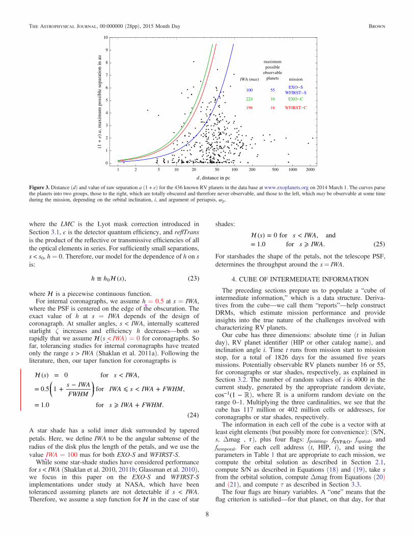
Table 6Tabular DRM for EXO-C

Planet Name Median Apparent Median Flux Median S/N Mission Day Union Cumulative UC Observing Cumulative Merit Function Median Search Median Spectroscopic

Separation s Ratio Δmag Completeness UC Time (days) Observing Time (days) (1/days) Exposure Time Exposure Time (days)

1 epsilon Eri b 0.533 19.9 8.0 790 0.999 1.00 0.502 0.5 1.991 0.00 0.042 mu Ara c 0.280 21.4 8.0 23 0.980 1.98 0.890 1.4 1.101 0.39 12.103 GJ 832 b 0.420 20.0 8.0 1157 0.981 2.96 1.166 2.6 0.841 0.67 18.764 HD 190360 b 0.250 21.2 8.0 938 0.975 3.94 1.420 4.0 0.687 0.90 31.725 47 UMa c 0.230 20.8 21.3 1183 0.942 4.88 1.659 5.6 0.568 1.16 42.216 HD 217107 c 0.238 21.6 10.0 111 0.914 5.79 6.940 12.6 0.132 6.44 242.077 GJ 849 b 0.228 19.8 10.9 1742 0.563 6.35 41.696 54.3 0.014 41.20 1660.238 upsilon And d 0.230 21.6 63.4 660 0.051 6.40 11.489 65.8 0.004 10.99 381.799 HD 154345 b 0.224 21.4 55.5 349 0.399 6.80 460.512 526.3 0.001 460.01 18625.9210 HD 39091 b 0.228 22.4 45.9 930 0.049 6.85 312.543 838.8 0.000 312.04 12188.1711 GJ 328 b L L L L L L L L L L L12 14 Her b L L L L L L L L L L L13 HD 134987 c L L L L L L L L L L L14 55 Cnc d L L L L L L L L L L L15 GJ 179 b L L L L L L L L L L L16 HD 87883 b L L L L L L L L L L L


19

TheAstro

physica

lJourn

al,

00:000000(28pp),

2015Month

Day

Brow

n

promising targets (low , say < 0.01) are removed fromconsideration, as they are in Figures 8–11. The dropped targetsare poor choices, either because they are too costly in observingtime—say more than 100 days for a high probability target (UC∼ 1), or because the observing time is reasonable (∼ 1 day) butthe probability of success finding the planet is too low (UC∼ 0.01)—or because of some combination in between. By thisargument, we exclude planets with from the graphical DRMs,but they remain included in the tabular DRMs.

To highlight the value of observational success, character-ized by UC, the graphical DRMs show explanets with UC⩾ 0.90 in green, and those with UC < 0.90 in red.

With these considerations in mind, we can proceed to interpretthe results in Tables 3–6 and Figures 8–11, in which observationsare listed or displayed in rank order according to .Still under the assumption of perfect knowledge of the RV

orbital parameters, Sections 5 and 6 reveal some of the basicnature of an initial observing program to characterize knownRV planets. From the illustrative cases in Figures 4–7, we learnthat there are typically only a few, often brief, windows inabsolute time (Julian days) in which a search observation canbe scheduled with high confidence of success. In other words,observations of known RV planets are time-critical andtherefore challenging to schedule. The preceding sections have

Figure 6. Completeness panel for 14 Her b observed byWFIRST-C. Plot 1A shows that 14 Her is located in the continuous viewing zone, at ecliptic latitude +63°. Plot1B shows that the long period of 14 Her b (1773 days) affords only one cycle of SVP&O > 0, in the range 400 < t < 1200 mission day. Comparing Plot 1B with Plot1D, we note the divot centered at t = 598 mission day, which is caused by the sole node crossing by 14 Her b during the five years mission. From Plot 1E, we see thata search observation with >90% probability of success must be scheduled between 750 and 900 mission day.

20


developed and illustrated the input information needed by thescheduling algorithm to build diagnostic DRMs—and whenactual operations begin, to provide important information foroptimizing the observing schedule.

We have studied the four missions on a basis as equal aspossible, for example, assuming a five years duration for allmissions. The sparse and spikey nature of RV-planet availabil-ities means that the total number of planets characterized may besignificantly reduced if the mission duration is reduced.

A corollary of “sparse and spikey” is that potentialscheduling conflicts are rare. For the coronagraphs, Figures 10and 11 show no conflicts. For the star-shade missions,Figures 8–9 show only two or three conflicts, which shouldbe easily resolvable by small tweaks to the observing times.For the star-shade missions, the exposure times are typically

much shorter than the setup time, which means that longerexposure times, achieving higher astrometric accuracy, can beincorporated with little time penalty. Nevertheless, sources of

Figure 7. Median panel for 14 Her b observed by WFIRST-C. Plots 2A and 2B reveal that the regions of value zero for SVP&OC in Figure 6, Plot 1B, are due toobscuration (s < IWA) not toΔmag >Δmag0. Plot 2D reveals an elevated S/N requirement (S/N > 8), due to the node crossing at t = 598 mission day, everywhere butin a narrow range around t = 900 mission days, and that a severe penalty would result if the search mission for 14 Her b were scheduled at different time frame. InSection 6, Table 6, line 3, we see that the scheduling algorithm chose 894 mission day to observe 14 Her b with WFIRST-C, when ∼ 0.71—consistent with Plot 2Ein this figure.

21


systematic errors may limit the astrometric accuracy achievablein practice.

We note the mostly short and inconspicuous dashed lines inFigures 8–11, particularly for the exoplanets with the highestmerit (green). These lines show the exposure times for follow-on spectroscopy, beginning immediately after locating theplanet in a search image. In most cases, the spectroscopicexposure will be easily accommodated.

7. UNCERTAINTIES IN RV ORBITAL PARAMETERS

For the DRM-related calculations in Sections 2–6, we needsufficiently accurate RV orbital parameters for at least two tasks.First, observers need accuracy to confidently plan and schedule

observations. If they do not know the orbit, they can predictneither where the planet is nor where will be in the future.Second, accuracy is needed for the job of estimating mp (idem sini) using Equation (9). If one does not know the orbit, one cannotsay what value of s would be produced by any value of i.Therefore, success at either critical task—planning or interpretingobservations—depends on sufficiently accurate values of the RVorbital parameters other than i, such as the parameters a, e, t, ωp,msini, and ms.In Sections 2–6, we have assumed that the orbital parameters

are known perfectly, with zero error. In this section, weexamine the effects of actual orbital uncertainties, based on theRV data sets currently available in the public archive at theNASA Exoplanet Science Institute (NExScI).

Figure 8. Graphical DRM for WFIRST-S. Numbered dots mark the value of the median merit function and the mission day of the search exposure with maximum, as selected by the scheduling algorithm. Green: targets with ⩾90% probability of success in mass determination, due to UC ⩾ 0.9. Red: riskier targets withUC < 0.9. The labeling numbers correspond to the row numbers in Table 3. A solid line, when it extends beyond the dot, gives the median exposure plus setup time ofthe search observation. Dashed lines show the median exposure time for the possible follow-on spectroscopic exposure. Long spectroscopic exposures may not betolerated, for example, by the pointing restrictions. In this plot, candidate observations are cut off at = 0.01min , but all results are reported in Table 3.

Figure 9. Graphical DRM for EXO-S. See the caption of Figure 8.

22


Figure 10. Graphical DRM for WFIRST-C. See the caption for Figure 8.

Figure 11. Graphical DRM for EXO-C. See the caption for Figure 8.

Figure 12. Best case. Fits to real and hypothetical RV data sets for GJ 676 A b.Black: real data points. Red/orange: fit to the real data. Blue: fits to 100hypothetical data sets. See Figure 20 for the performance of Equation (9) as anestimator of mp for this exoplanet, with and without orbital errors.

Figure 13. Second-best case. Fits to real and hypothetical RV data sets for 16 CygB b. See caption to Figure 12. See Figure 21 for the performance of Equation (9)as an estimator of mp for this exoplanet, with and without orbital errors.

23


To learn how orbital uncertainties impact the estimation ofms, we selected a sample of the input catalog using four criteria:the selected exoplanets (1) are valid (observable outsideIWA = 0″.100), (2) are currently thought to be single-planetsystems, (3) have RV data sets available for download from the

NExScI archive, and (4) have no known complications fromstellar companions (e.g., not gamma Cep b, not HD 196885 b).Some 21 of the 55 RV exoplanets meet the criteria: epsilon Erib, HD 10647 b, GJ 832 b, 7 CMa b, 14 Her b, HD 147513 b,HD 154345 b, GJ 649 b, GJ 849 b, HD 87883 b, GJ 676 A b,

Figure 14. Third-best case. Fits to real and hypothetical RV data sets for 14Her b. See Figure 22 for the performance of Equation (9) as an estimator of mp

for this exoplanet, with and without orbital errors. See caption to Figure 12.

Figure 15. Fourth-best case. Fits to real and hypothetical RV data sets for 7CMa b. See Figure 23 for the performance of Equation (9) as an estimator ofmp for this exoplanet, with and without orbital errors. See caption to Figure 12.

Figure 16. Fifth-best case. Fits to real and hypothetical RV data sets for HD50554 b. See Figure 24 for the performance of Equation (9) as an estimator ofmp for this exoplanet, with and without orbital errors. See caption to Figure 12.

Figure 17. Sixth-best case. Fits to real and hypothetical RV data sets for GJ179 b. See Figure 25 for the performance of Equation (9) as an estimator of mp

for this exoplanet, with and without orbital errors. See caption to Figure 12.

Figure 18. Second-worst case. Fits to real and hypothetical RV data sets forepsilon Eri b. See Figure 26 for the performance of Equation (9) as anestimator of mp for this exoplanet, with and without orbital errors. See captionto Figure 12.

Figure 19. Worst case. Fits to real and hypothetical RV data sets for GJ 832 b.See Figure 27 for the performance of Equation (9) as an estimator of mp for thisexoplanet, with and without orbital errors. See caption to Figure 12.

24


Original Text

IWA=0100),

HD 216437 b, HD 117207 b, HD 30562 b, 16 Cyg B b, HD70642 b, HD 39091 b, GJ 179 b, HD 50554 b, HD 142022 b,and GJ 317 b.

In this error analysis, we must take into account that orbitalparameters are not independent but have finite covariance. Thismeans that the uncertainties in the parameters cannot bepropagated or combined in quadrature in the usual way.Instead, we use a technique that Brown (2004) applies to RVdata sets, calling it “Monte Carlo projection.” Press et al.(2007; Section 15.6) explain and justify this technique ingeneral terms. In the current application, this technique usesEquation (9) to produce a large sample of mp from a largesample of hypothetical RV data sets and a large sample of s.

Figure 20. Best case: GJ 676 A b. Performance of Equation (9) as an estimatorof mp. No evidence of bias or broadening due to orbital errors. Red/orange andpurple: astrometric errors in s only. Note that the fractional error in mp isapproximately 0.1 for only astrometric errors in s, as expected from thespecification in Equation (1). Blue and purple: performance due to bothastrometric and orbital uncertainties. To the degree that performance profiles ofthe two estimators coincide, the orbital uncertainties do not degrade theperformance of Equation (9). The indicated values of the mean and standard ofmp refer to the case of astrometric errors only. “% valid shown” refers to thepercentage of the results for mp from the 2000 hypothetical orbits that fall in therange of the histogram. The values s = 0″.105, t = 1733 mission day, and S/N = 15.6 are typical of this exoplanet in EXO-S DRMs. See Figure 12 for theRV data and orbital fits.

Figure 21. Second-best case: 16 Cyg B b. Blue: no evidence of bias orbroadening of the distribution due to orbit errors. See caption to Figure 20. Thevalues s = 0″.115, t = 1067 mission day, S/N = 21.9 are typical of thisexoplanet in EXO-S DRMs. See Figure 13 for the RV data and orbital fits forthis exoplanet.

Figure 22. Third-best case: 14 Her b. Blue: orbital errors bias the estimationsof mp to lower values, without broadening. See caption to Figure 20. Thevalues s = 0″.169, t = 1043 mission day, and S/N = 8 are typical of thisexoplanet in EXO-S DRMs. Because S/N = 8, which is the noise floor,Equations (18) and (19) have increased S/N from the value required byEquation (1), with the result that Fmp < 0.1, and in this case Fmp = 0.0811. SeeFigure 14 for the RV data and orbital fits.

Figure 23. Fourth-best case: 7 CMa b. Orbital errors bias and broaden theestimations of mp. See caption to Figure 20. The values s = 0″.101, t = 180mission day, and S/N = 120.8 are typical of this exoplanet in EXO-S DRMs.See Figure 15 for the RV data and orbital fits.

Figure 24. Fifth-best case: HD 50554b. Blue: orbital errors bias and broadenthe estimations of mp. See caption to Figure 20. The values s = 0″.100, t = 843mission day, and S/N = 53.9 are typical of this exoplanet in EXO-S DRMs. SeeFigure 16 for the RV data and orbital fits.

25


We develop the latter sample is by 106 draws from a normalrandom deviate of mean equal to the measured value of s andstandard deviation σs from Equation (12).

We develop the former sample by Monte Carlo projection.Let us assume the existing, real RV data set is

δt u u{{ , , },...}j j j , with one data triplet for each measurement.

The time of the jth data point is tj (JD), the measured RV is uj,and the uncertainty in uj is δu j. A hypothetical data set is {{tj,uuj, δ uj}, ...}, where uuj is a random number drawn from thenormal distribution with mean uj and standard deviation δu j.Following the justification of Press et al. (2007), we assumethat such a hypothetical data set is statistically equivalent to thereal data set, and that when we fit a hypothetical data set for theorbital parameters, the results are statistically equivalent tothose produced by fitting the real data set.The needed sample of mp results from fitting the sample of

hypothetical data sets for RV orbital solutions. We use thefitted values to compute sin i for s using Equation (9), and thenmp from the fitted value of msini. We perform this operation forall 21 exoplanets in the working sample.Figures 12–19 show, in red, the least-squares fits to the real

data sets for 8 of 21 exoplanets in the sample. Also, in blue, arefits to 100 hypothetical data sets for each exoplanet. We rated thefirst six exoplanets in these figures as “best to the eye.” The lasttwo of the eight exoplanets (epsilon Eri b and GJ 832 b) show theworst two performances by eye. The corresponding results for all21 exoplanets in the working sample are available for down-loading at http://www.stsci.edu/∼RAB/RV%20Graphics/, withthe file name “AllFourUps.pdf.”We must now relate the diversity of the hypothetical fits

documented in Figures 12–19, to the performance ofEquation (9) as an estimator of mp. For each exoplanet in theworking sample of 21, we compute dual histograms, shown inFigures 20–26. (These histograms are also included in“AllFourUps.pdf.”) The abscissa of the historams is the valueof mp inferred from an RV data set for an arbitrary value of s.The ordinate is the empirical probability of mp falling in a givenhistogram bin.The histograms show that only in 2 of 21 cases—GJ 676 A b

and 16 Cyg B b—could mp be estimated with ⩾10% accuracyby Equation (9). Only for those two exoplanets is the estimatorreasonably accurate and seemingly unbiased.According to the DRMs, only the two star-shade missions—

and not the two coronagraph missions—could observe GJ676 A b and 16 Cyg B b.The last line of Table 7 gives the number of unevaluated RV

exoplanets, which are still in play after the 21 exoplanets justtreated have been retired, and after those with low UC or low

Figure 25. Sixth-best case: GJ 179 b. Blue: orbital errors skew and broaden theestimations of mp. See caption to Figure 20. The values s = 0″.133, t = 200mission day, and S/N = 8 are typical of this exoplanet in EXO-S DRMs. SeeFigure 17 for the RV data and orbital fits.

Figure 26. Next-to-worst case: epsilon Eri b. Blue: orbital errors skew andbroaden the estimations of mp. See caption to Figure 20. The values s = 0″.560,t = 812 mission day, and S/N = 8 are typical of this exoplanet in EXO-SDRMs. See Figure 18 for the RV data and orbital fits.

Table 7Number of High-priority Exoplanets Not yet Evaluated

as EstimatorsQ2 of True Mass

Case WFIRST-S WFIRST-C EXO-S EXO-C

All valid planets 45 12 37 10After removing evaluated

estimators of mp

26 6 18 5

After removing < 0.01 orUC < 0.90

22 5 14 4

Note. Valid planets are those listed without ellipses in Tables 3–7. The 19 of 21exoplanets that are poor estimators of mp are epsilon Eri b, HD 10647 b, GJ832 b, 7 CMa b, 14 Her b, HD 147513 b, HD 154345 b, GJ 649 b, GJ 849 b,HD 87883 b, HD 216437 b, HD 117207 b, HD 30562 b, HD 70642 b, HD39091 b, GJ 179 b, HD 50554 b, HD 142022 b, and GJ 317 b. The exoplanetswith ⩾ 0.01 and UC ⩾ 0.90 are those with green dots in Figures 8–11.

Figure 27. Worst case: GJ 832 b. Blue: orbital errors skew and broaden theestimations of mp. See caption to Figure 20. The values s = 0″.346, t = 1041mission day, and S/N = 8 are typical of this exoplanet in EXO-S DRMs. SeeFigure 19 for the RV data and orbital fits.

26


http://www.stsci.edu/<RAB/RV%20Graphics/

have been removed, as discussed in Section 6. The 22 uniqueexoplanets in the last line of Table 7 are: 47 UMa b, 47 UMa c,beta Gem b, gamma Cep b, HD 128311 c, HD 134987 c, HD13931 b, HD 169830 c, HD 181433 d, HD 190360 b, HD192310 c, HD 196885 b, HD 204941 b, HD 217107 c, HD222155 b, HD 33636 b, HD 38529 c, HD 7449 b, HD 89307 b,mu Ara b, mu Ara c, and upsilon And d.

We can use the binomial distribution to estimate the numberof unevaluated exoplanets expected to be acceptable estimatorsof mp We assume the probability of a good estimator isprob = 0.0952 = −1 19 21, the probability found in thesample of 21 evaluated exoplanets. That is, there seems to beno reason to think that the 22 so far unevaluated exoplanets aredrawn from a different population of mp estimators than theearlier 21. Under the assumption that the parent distribution isthe same for two sets, the number of good estimators in a set ofnp = 4, 5, 14, or 22 RV planets is given by the binomialdistribution with parameters prob and np. The results are shownin Figure 28.

8. SUMMARY AND CONCLUSIONS

In Sections 2–5, operating under the assumption that wehave perfect knowledge of the RV orbital parameters, wederive an analytic framework for the accuracy of an RVplanet’s true mass estimated by direct astrometry on high-dynamic-range images. The analysis involves the RV orbitalparameters, specifications of the telescope, random values ofthe unknown inclination angle, and science operations—mostnotably the scheduling algorithm, merit function, and exposuretime. We have empirically derived the S/N needed to achieve adesired astrometric accuracy, which is ±10% in the currenttreatment. We assume that the observations use a diffraction-limited, background-dominated telescope in space. Our treat-ment includes node crossings, solar and anti-solar pointingrestrictions, photometric and obscurational completeness,exposure-time availability, and image blurring due to orbital

motion, but Sections 2–5 do not include uncertainties in the RVorbital parameters.In Section 6, still ignoring the issue of orbital uncertainties,

we build DRMs for four missions under current study atNASA. The science drivers for these missions includeestimation of the true mass of known RV exoplanets by meansof direct astrometry. For both coronagraphs, the input catalogincludes 16 RV planets, of which EXO-C could possiblyobserve 10, of which 6 would have a 90% probability ofsuccess. Of the same 16 planets, WFIRST-C could possiblyobserve 12, of which 9 are high-probability. For both star-shademissions, the input catalog includes 55 planets, of which EXO-S could possibly observe 37, of which 20 are high priority. Ofthe same 55, WFIRST-S could possibly observe 45, of which30 are high-probability.In Section 7, we introduce current uncertainties in the RV

orbital parameters. This inclusion reveals that the orbitaluncertainties have a major negative impact on the observingprogram for estimating the true planetary mass.For the coronagraphs, WFIRST-C and EXO-C, the most

likely number of good estimators of mp among the 55 RVplanets in the input catalog is zero.For the star shades, EXO-S and WFIRST-S, the most likely

numbers of good estimators are three and four, respectively,counting GJ 676 A b and 16 Cyg B b.For over two decades, achieving meaningful estimates of the

true masses of known RV planets has been an important goal ofexoplanetary researchers. This aspiration has been a majorscience motivator for the four missions under study. We nowknow that even with additional direct imaging observationsfrom the missions examined here, current RV measurementuncertainties prevent us from achieving the desired massprecision.Uncertain orbital elements undermine all programs of direct

imaging and spectroscopy of RV exoplanets. This is because allthose programs call for accurate planning of the pointing andtiming of the telescope. We have looked closely only at the task

Figure 28. Estimated number of unevaluated RV exoplanets that will turn out to be good estimators of mp, according to the binomial distribution with parametersprob = 0.0952 and np listed in the legend. For the coronagraphs, WFIRST-C and EXO-C, zero is the most likely number of good estimators of mp among the 55 RVplanets in the input catalog. For the star shades, EXO-S andWFIRST-S, the most likely numbers of good estimators are three and four, respectively, counting GJ 676 Ab and 16 Cyg B b.

27


of true-mass estimation, but there can be no doubt that thescope of the issue is broader and deeper (Brown et al. 2007).The impact is exacerbated for barely unresolved orbits withperiods of years. The exoplanet will barely clear the centralfield obscuration—at some time, maybe, but when and where?

We call for a concerted effort to improve RV orbitalparameters adequately to support unbiased, accurate estimationof mp for a meaningful number of RV exoplanets. Until wehave identified many more mass estimators that perform as wellas GJ 676 A b and 16 Cyg B b seem to do, the goal ofestimating the true masses of a significant number of knownRV exoplanets will lie beyond reach.

We are grateful for Stuart Shaklan’s interest in andencouragement of this research. Thanks to Marc Postman forsupport and guidance. We thank John Krist for helpful input onWFIRST-C. Thanks to Mark Marley and Jack Lissauer forinputs on the science program related to known RV planets.This research has made use of the Exoplanet Orbit Databaseand the Exoplanet Data Explorer at exoplanets.org, and thearchive at the NASA Exoplanet Science Institute (NExScI).Many thanks to Jason Wright for help understanding and usingthe archives.

REFERENCES

Burrows, C. J. 2003, in The Design and Construction of Large OpticalTelescopes, ed. P. Y. Bely (New York: Springer), 433

Burrows, C. J., Brown, R. A., & Sabatke, E. M. 2006, Aberrational DeltaMagnitude, manuscript; http://www.stsci.edu/~RAB/papers/WFC_ICS_Final_Report.pdf

Brown, R. A., Shaklan, S. B., & Hunyadi, S. L. 2007, Science Operations andthe Minimum Scale of TPF, JPL 07–02 7/07

Brown, R. A. 2004, ApJ, 607, 1079Brown, R. A. 2005, ApJ, 624, 1010Brown, R. A. 2009, ApJ, 702, 1237Brown, R. A. 2011, ApJ, 733, 68Brown, R. A. 2014, ApJ, 788, 192Brown, R. A. 2015, ApJ, 799, 87Brown, R. A., & Soummer, R. 2010, ApJ, 715, 122Chandrasekhar, S., & Münch, G. 1950, ApJ, 111, 142Des Marais, D. J., Harwit, M., Jucks, K., et al. 2002, AsBio, 2, 153Dumusque, X. 2014, ApJ, 796, 133Giannini, E., & Lunine, J. I. 2013, RPPh, 76, 056901Glassman, K., Johnston, A., Lo, A., et al. 2010, in Proc. SPIE Q1, 7731, 773150Ho, S., & Turner, E. L. 2011, ApJ, 739, 26Jorisson, A., Mayor, M., & Udry, S. 2001, A&A, 379, 992Lopez, S., & Jenkins, J. S. 2012, ApJ, 756, 177Maire, A.-L., Galicher, R., Boccaletti, A., et al. 2012, A&A, 541, A83Marcy, G. W., Butler, R. P., Fischer, D., et al. 2005, PThPS, 158, 24Müller, M., & Weigelt, G. 1987, A&A, 175, 312Press, W. H., Flannery, B. P., Teukolsky, S. A., & Vetterling, W. T. 2007,

Numerical Recipes (3rd ed.; New York: Cambridge Univ. Press)Seager, S., et al. 2015, ExoS: Starshade Probe-Class, Exoplanet Direct Imaging

Mission Concept, Final Report, https://exep.jpl.nasa.gov/stdt/Exo-S_Starshade_Probe_Class_Final_Report_150312_URS250118.pdf

Reid, I. N., http://www.stsci.edu/~inr/phot/allphotpi.sing.2massShaklan, S. B., Noecker, H. C., et al. 2010, Proc. SPIE, 7731, 77312GShaklan, S. B., Marchen, L., et al. 2011a, Proc. SPIE, 8151, 815109Shaklan, S. B., Marchen, L., et al. 2011b, Proc. SPIE, 8151, 815113Spergel, D., Gehrels, N., et al. 2015, Wide-Field InfraRed Survey Telescope–

WFIRST-AFTA, 2015 Report, http://exep.jpl.nasa.gov/wfirst-afta/WFIRST–AFTA_SDT_Report_150310_Final.pdf Q2

Stapelfeldt, K., et al. 2015, Exo-C: Imaging Nearby Worlds, Final Report,https://exep.jpl.nasa.gov/stdt/Exo-C_Final_Report_for_Unlimited_Release_150323.pdf

Traub, W. A., Belikov, R., et al. 2014, Proc. SPIE., 9143, 91430NUdry, S., & Santos, N. C. 2007, ARA&A, 47, 397Zucker, S., & Mazeh, T. 2001, ApJ, 562, 1038

28


http://www.stsci.edu/~RAB/papers/WFC_ICS_Final_Report.pdf

http://www.stsci.edu/~RAB/papers/WFC_ICS_Final_Report.pdf

http://dx.doi.org/10.1086/421896

http://adsabs.harvard.edu/abs/2004ApJ...610.1079B

http://dx.doi.org/10.1086/429124


http://dx.doi.org/10.1088/0004-637X/702/2/1237


http://dx.doi.org/10.1088/0004-637X/733/1/68

http://adsabs.harvard.edu/abs/2011ApJ...733...68B

http://dx.doi.org/10.1088/0004-637X/788/2/192

http://adsabs.harvard.edu/abs/2014ApJ...788..192B

http://dx.doi.org/10.1088/0004-637X/799/1/87

http://adsabs.harvard.edu/abs/2015ApJ...799...87B

http://dx.doi.org/10.1088/0004-637X/715/1/122

http://adsabs.harvard.edu/abs/2010ApJ...715..122B

http://dx.doi.org/10.1086/145245

http://adsabs.harvard.edu/abs/1950ApJ...111..142C

http://dx.doi.org/10.1089/15311070260192246

http://adsabs.harvard.edu/abs/2002AsBio...2..153D

http://dx.doi.org/10.1088/0004-637X/796/2/133

http://adsabs.harvard.edu/abs/2014ApJ...796..133D

http://dx.doi.org/10.1088/0034-4885/76/5/056901

http://adsabs.harvard.edu/abs/2013RPPh...76e6901G

http://dx.doi.org/10.1088/0004-637X/739/1/26

http://adsabs.harvard.edu/abs/2011ApJ...739...26H

http://dx.doi.org/10.1051/0004-6361:20011373

http://adsabs.harvard.edu/abs/2001A&A...379..992J

http://dx.doi.org/10.1088/0004-637X/756/2/177

http://adsabs.harvard.edu/abs/2012ApJ...756..177L

http://dx.doi.org/10.1051/0004-6361/201218954

http://adsabs.harvard.edu/abs/2012A&A...541A..83M

http://dx.doi.org/10.1143/PTPS.158.24

http://adsabs.harvard.edu/abs/2005PThPS.158...24M

http://adsabs.harvard.edu/abs/1987A&A...175..312M

https://exep.jpl.nasa.gov/stdt/Exo-S_Starshade_Probe_Class_Final_Report_150312_URS250118.pdf

https://exep.jpl.nasa.gov/stdt/Exo-S_Starshade_Probe_Class_Final_Report_150312_URS250118.pdf

http://www.stsci.edu/~inr/phot/allphotpi.sing.2mass

http://dx.doi.org/10.1117/12.857591

http://adsabs.harvard.edu/abs/2010SPIE.7731E..2GS

http://dx.doi.org/10.1117/12.892838

http://dx.doi.org/10.1117/12.892834

http://exep.jpl.nasa.gov/wfirst-afta/WFIRST�AFTA_SDT_Report_150310_Final.pdf

http://exep.jpl.nasa.gov/wfirst-afta/WFIRST�AFTA_SDT_Report_150310_Final.pdf

https://exep.jpl.nasa.gov/stdt/Exo-C_Final_Report_for_Unlimited_Release_150323.pdf

https://exep.jpl.nasa.gov/stdt/Exo-C_Final_Report_for_Unlimited_Release_150323.pdf

http://dx.doi.org/10.1117/12.2054834

http://adsabs.harvard.edu/abs/2014SPIE.9143E..0NT

http://dx.doi.org/10.1146/annurev.astro.45.051806.110529

http://adsabs.harvard.edu/abs/2007ARA&A..45..397U

http://dx.doi.org/10.1086/323866

http://adsabs.harvard.edu/abs/2001ApJ...562.1038Z

TRUE MASSES OF RADIAL-VELOCITY EXOPLANETS

Documents

Transcript of TRUE MASSES OF RADIAL-VELOCITY EXOPLANETS