Tropospheric Halogens - Effect on Ozone · Title Tropospheric Halogens Effect on Ozone Objectives:...

Tropospheric Halogens - Effect on Ozone

Project: EVK2-CT-2001-00104

THALOZ Web page: http://www.atm.ch.cam.ac.uk/~thaloz

Final Report: 1st Feb 2002 – 30th Apr 2005

SECTIONS: 5 - 6

Co-ordinator: Dr R.A. Cox

(University of Cambridge, UK)

Participants Information: No Institution /

Organisation Street name and number

Post Code

Town / City Country Code

Title Family Name

First Name

Telephone No

Fax No E-mail

Dr Cox Richard (44) 1223336253

(44) 1223 336362

[email protected] 1 Dept of Chemistry,University of Cambridge

Lensfield Rd

CB2 1EW Cambridge UK

Prof. Pyle John (44) 1223 336473

(44) 1223 336362

[email protected]

2 Institute ofEnvironmental Physics and Remote Sensing IUP/IFE, University of Bremen

Postfach 330440

28334 Bremen D Dr Burrows JohnPhilip

(49) 421 218 4548

(49) 421 218 4555

[email protected]

Prof. Plane John (44) 1603592108

(44) 1603 507719

[email protected] 3 School of EnvironmentalScience, University of East Anglia

NR4 7TJ Norwich UK

Prof. Liss Peter (44) 1603 592563

(44) 1603 507719

P. [email protected]

4 Max-Planck-Institut fürChemie, Division of Atmospheric Chemistry

Postfach 3060

55020 Mainz D Dr Crowley John (49) 6131305474

(49) 6131 305436

[email protected]

5 Laboratoire de Pollution Atmosphérique, Ecole Polytechnique Fédérale de Lausanne EPFL.

CH-1015 LAUSANNE CH Dr Rossi Michel (41) 21 6935321

(41) 21 693 36 26

[email protected]

SECTION 5: EXECUTIVE PUBLISHABLE SUMMARY, RELATED TO THE OVERALL PROJECT DURATION

Contract n° EVK2-CT-2001-00104 Project Duration: 3 years 3 months Title Tropospheric Halogens Effect on Ozone Objectives: The overall objective of THALOZ has been to further our understanding of the influence of halogens on tropospheric ozone and tropospheric oxidation chemistry, and their consequent influence on radiative forcing of climate by greenhouse gases. Specifically it was aimed to provide key data relating the sources, distribution and chemical reactions of reactive halogen in the troposphere; to evaluate the global and regional influence of halogens on tropospheric ozone and to determine the influence of halogen chemistry on radiative forcing of climate. The emphasis has been on reactive Br and I compounds (e.g. BrO, IO) because they have greatest potential for ozone depletion in the troposphere. Scientific achievements: Major progress was made in extending knowledge of halogen species in the troposphere. The analysis of BrO global climatology from GOME and SCIAMACHY satellite data has established a time series for BrO from 1995 – 2005. Free tropospheric BrO amounts, are deduced to be slightly lower than earlier estimates and the presence of high BrO mixing ratios in the lower troposphere, in springtime, in both Polar regions has been confirmed. Ground based remote sensing measurements have confirmed that BrO and IO are widely present in the troposphere. IO is mainly found in the marine boundary layer and BrO occurs over salt lakes, over marginal ice zones in N and S Polar regions, in the marine boundary layer and in some volcanic plumes. Iodine containing molecules, OIO and I2, have been observed in the atmosphere for the first time. A major focus has been halogen activation from sea salt aerosol by heterogeneous reaction chemistry. Laboratory studies of activation from sea salt have shown that both HOBr and HOI activate Br before Cl; rates are pH dependent and the mechanisms deduced are consistent with observed Br- deficits in the marine aerosol. A new source of inorganic Br from sea spray has been quantified, on the basis of observed Br- deficits in the marine aerosol. This source is dominant in the lower troposphere and contributes significantly to the global Br budget. ‘Frost flowers’, i.e. brine coated ice crystals have been identified as source of reactive Br, which can explain the time and location of a large anomaly in BrO concentrations in the polar lower troposphere. Important new information on the kinetics and photochemistry of iodine species shows that ozone loss is less sensitive to iodine, compared to bromine, because of the formation of iodine oxides. This information is also relevant for the emerging issue of aerosol formation from iodine oxides. In the open ocean iodocarbon release is constrained by photochemical modification in seawater. Emission of highly reactive iodine compounds from inshore and inter-tidal regions can be larger, and include release of molecular I2. The modelling effort was directed mainly at global bromine chemistry and its effect on ozone. A new 3-D model with sources and sinks of bromine species has been formulated, which allows calculation of global seasonal, latitudinal and height distributions of total inorganic bromine (Brx) and partitioned species. Bromocarbons provide the main source of upper tropospheric Brx and sea salt derived Brx dominates the lower troposphere, especially in the Southern Hemisphere. The main result of this study is to show that the amount of bromine cycled through the troposphere is larger than previously believed, due partly to a significant new source from natural marine aerosol. There are strong regional differences in the Br enhancement, which occurs mainly at high latitudes. Reactive Brx leads to a significant new loss term in the tropospheric ozone budget in the contemporary atmosphere. The 3D-model calculations predict lower ozone concentrations (5-10% reduction) in most regions, except for the tropics. The effect is due to direct O3 loss by Br reactions and also reduced O3 production as a result of NO2 removal via bromine nitrate hydrolysis. Ozone fields are still consistent with observed climatology of tropospheric ozone. The calculations do not include any impact on ozone due to reactive Cl and I species or the specific bromine source related to frost flower episodes.

Clear evidence for ozone loss due to reactive halogens is now apparent in local observations, both in the polar tropospheric BL and at coastal observatories in remote locations in the W. Pacific and Southern Ocean. Detailed models of local MBL halogen chemistry confirm the chemical origin of local ozone loss. Radiative forcing of climate due to modelled contemporary ozone is decreased by 0.1 Wm-2 when bromine chemistry is included. The absence of any trends in BrO amounts suggest that this contribution is not changing at present.

Main deliverables:

1. Maps of global distribution of BrO column-amounts since 1995, from GOME and SCIAMACHY satellite data; and measurements of key species in the MBL and from the BREDOM network. 2. Quantitative source terms have been derived for naturally occurring bromocarbons and iodocarbons, and for inorganic bromine from marine aerosols. 3. Compilation of evaluated data on the key chemical reactions controlling the impact of reactive halogens on atmospheric composition, based on new laboratory studies of reaction kinetics and photochemistry. 4. New numerical models describing atmospheric composition, including a 3-D chemical transport model with halogen chemistry and simple models of complex chemistry in the atmospheric boundary layer and upper surfaces of the ocean. 5. Predicted regional and global distribution and budgets of bromine compounds. 6. Predicted effects of bromine compounds on ozone in the contemporary troposphere. 7. Changes in calculated radiative forcing due to the current amounts of bromine in the troposphere.

Socio-economic relevance and policy implications: The development of improved methodology for retrieval of geophysical information from satellite datasets adds value to the investment in EO technology, with potential benefits to other sectors, including monitoring of air pollution and extreme events. Policy for regulation of bromine compounds in the frame of the Montreal Protocol for protection of the ozone layer will be aided by more reliable estimates of the total natural bromine emissions and their tropospheric distribution. The role of short-lived halogen carriers, in transporting ozone-depleting halogens to the stratosphere, is currently being assessed in the WMO Ozone Assessment due to be completed in 2006. The significant changes in calculated radiative forcing due to the effect of current amounts of halogens on tropospheric ozone will need to be considered in the IPCC scientific assessment of future climate change.

Conclusions: The THALOZ programme has successfully carried out the original aims to provide key data relating the sources, distribution and chemical reactions of reactive halogen in the troposphere; to evaluate the global and regional influence of halogens on tropospheric ozone and to determine the influence of halogen chemistry on radiative forcing of climate. The information obtained provides an improved quantitative understanding of the role of halogen compounds in controlling the composition of the troposphere. Naturally occurring bromide compounds have a significant influence on ozone amounts and consequently on oxidising capacity. The biogeochemical cycling of iodine is now better known. There are potentially significant impacts of these findings on the radiative forcing of climate.

Dissemination of results: The results of this work will be disseminated through publication of scientific papers and in published material from assessments, reviews and media presentations. In the near term information is disseminated via web-based channels such as: a metadata archive of reactive halogen chemistry; analysed GOME and SCIAMACHY fields and IUPAC Evaluated kinetic data for atmospheric chemistry.

Keywords: ATMOSPHERIC COMPOSITION; BIOGEOCHEMICAL CYCLES; TROPOSPHERIC HALOGENS; OZONE; CHEMISTRY-CLIMATE COUPLING; BROMINE; IODINE.

2

SECTION 6: DETAILED REPORT, RELATED TO OVERALL PROJECT DURATION

1. Background

THALOZ was designed and carried out as a concerted, multidisciplinary effort aimed at understanding the effect of reactive halogens on tropospheric ozone and tropospheric oxidation chemistry, and the consequent influence on radiative forcing of climate. The work plan combined use of DOAS observations (satellite and ground-based), laboratory studies, model development and model application.

Halogens are released into the troposphere from the photochemical breakdown of organo-halogens, both natural and anthropogenic, and from the oxidation of Cl- and Br- in sea salt. Halogens released into the troposphere result in catalytic destruction of tropospheric ozone, with consequent effects on the chemistry controlling atmospheric oxidation and composition. Destruction involving I and Br atom cycles are particularly efficient. Cl and Br atoms react to remove organic pollutants from the atmosphere, and so contribute to the oxidation capacity. It is essential to have an understanding of the role of halogens in tropospheric chemistry, in order to assess the oxidative potential of the troposphere, the tropospheric budget of ozone and of the reactive greenhouse gases. Previous EU framework research has contributed substantially to the body of knowledge of tropospheric halogens; this study aimed to exploit and advance this knowledge and establish the effects of halogens on global tropospheric chemistry, as it affects climate forcing.

2. Scientific/technological and socio-economic objectives

2.1 Scientific Objectives

The specific objectives of the proposed work and the questions, which have been addressed are summarised below:

Distribution of reactive halogen species in the troposphere: The THALOZ programme aimed to determine the geographical and seasonal distribution of reactive halogens and precursors for reactive halogens by analysis and critical evaluation of data from existing and future remote sensing and in-situ measurements. It was planned to use ground based remote sensing data from several locations, coupled with the global data from the GOME and SCIAMACHY instruments aboard the ESR-2 and ENVISAT satellites (the latter was launched during the first year of THALOZ). The focus has been on the halogen oxides BrO and IO. These data add to the increasing pool of observations of reactive BrO in the troposphere, including over salt lakes, over marginal ice zones in N and S Polar regions, in the marine boundary layer and in volcanic plumes. In addition, IO, OIO and I2 have been measured at coastal sites in the Northern and Southern Hemispheres. ClO has also been observed over salt lakes and in volcanic plumes.

In this context, very accurate, high spectral resolution laboratory investigations of the absorption cross sections of the halogen oxides were also required.

To provide key data relating to sources and sinks of reactive halogens: Halogens are released into the troposphere from the photochemical breakdown of organo-halogens and

3

from the oxidation of Cl- and Br- in sea salt aerosol. These sources were to be investigated during THALOZ. Laboratory investigation of the halogen chemistry leading to the release of reactive halogen was planned together with laboratory investigations of the marine organo-halogen source. Both source strengths and distributions were to be studied using models of atmospheric chemistry. A particular process for the release of sea salt bromide, enabled through the formation of frost flowers, i.e. brine coated ice crystals, in Polar regions has been studied in detail both using satellite measurements and models. Measurements have also identified volcanoes as a new source of reactive bromine, during the course of the programme, and a survey to identify the likely source strength has been carried out.

Gas phase photochemistry: In order to understand sinks of reactive halogens and their effect on other atmospheric constituents (primarily ozone), a number of laboratory experiments were planned, focussing on iodine species, for which there were a number of unanswered questions. Studies of the photolysis cross-sections of BrO and a number of iodine species, were planned in order to understand photolysis rates and product distributions, as well as being able to use new high-resolution spectra for field observations and laboratory experiments. A number of kinetic studies involving iodine oxides were also planned. During the course of the programme, it became apparent that the work on iodine oxides is highly relevant in the formation of nanoparticles in the marine environment and, hence, has climate implications.

To construct a budget for tropospheric halogens: the THALOZ programme planned to obtain a quantitative knowledge of the production and loss process, combined with state-of-the-art global models and with the observed distributions of reactive halogens to determine the total fluxes of the active halogen in the atmosphere. This budget will determine whether our current understanding of the sources of tropospheric halogen oxides is adequate and the extent to which the observed concentrations of reactive halogens are due to natural processes or result from anthropogenic activity. This part of the programme has been successfully carried out for reactive bromine compounds (and methyl bromide).

To evaluate the global and regional influence of halogens on tropospheric ozone: the impact of reactive halogens on amounts and distribution of ozone was to be assessed with the emphasis on regional episodic effects and on the overall budget of tropospheric ozone. Observations and model studies have been used to this effect.

To determine the influence of reactive halogen chemistry on radiative forcing due to reactive greenhouse gases: future concentrations of greenhouse gases depend on the evolution of tropospheric oxidation capacity. Reactive halogens affect tropospheric oxidation capacity directly and via their effect on tropospheric ozone and, hence, will affect radiative forcing due to modification of reactive greenhouse gas concentrations. The effect on tropospheric ozone and the consequent radiative forcing has been calculated.

2.2 Technological Objectives:

A number of technological advances were planned for the THALOZ programme these included:

A new atmospheric observation programme for BrO. New data analysis techniques were required for the new satellite instrument SCIAMACHY, which was launched on ENVISAT,

4

in the first year of the project. Continued analysis of the older satellite-based GOME instrument was also required by the programme. Significant reworking of the data retrieval was needed in order to maintain a good level of data quality. A new network of ground-based DOAS instruments was also planned. All of this work was to be carried out by Partner 2.

Installation and implementation of new equipment in laboratories. A chemical ionisation mass spectrometer was to be commissioned for this project along with two aerosol flow tube systems constructed specifically for THALOZ.

Development of models of halogen chemistry. In the initial stages of this work a box-model of halogen chemistry (chlorine, bromine and iodine) was to be developed by Partner 1. Appropriate sub-sets of the full halogen chemistry scheme were then to be implemented in global CTMs.

2.3 Socio-Economic Objectives:

The results of the research were designed to help enhance the quality of life and health, by the preservation of the environment in European countries. The EU is developing Europe-wide policy on this issue through its participation in the intergovernmental panel on climate change (IPCC), which supports the UN Kyoto Protocol and the UNEP-WMO Scientific Assessment of Ozone Depletion, which in turn supports the Parties to the UN Montreal Protocol. All European countries and the EU have agreed to abide by the Copenhagen agreement on ozone depleting substances and the Kyoto and Buenos Aires agreements on greenhouse gases. These require inventories of production and fluxes of relevant trace constituents to be established and managed (see for example: COM (96)557, COM (97)481, COM (98)353, COM (98)108, Dec 93/389).

2.4 Programme Implementation

In order to meet the above aims, the project was broken down into a number of work packages, each of which contributed to at least one deliverable. In producing the final deliverables, collaboration has been required between the different groups working on laboratory measurements, field data and model simulations.

Work Package Data: This work package was designed to deliver a comprehensive compilation of data and metadata for halogen species in the troposphere (Partners 1 and 2).

Laboratory Work Packages L1, L2 and L3 were designed to deliver a compilation of kinetic and mechanistic data for tropospheric halogen chemistry. In the areas of gas-phase chemistry (L1, Partners 2, 3 and 4), heterogeneous chemistry, releasing reactive halogens from sea salt, (L2, Partners 1 and 5) and halogen chemistry in seawater (L3, Partner 3).

The modelling Work Packages were designed to deliver a comprehensive gas-phase box model for tropospheric halogen chemistry (M1); a compilation of budgets and life-cycles of tropospheric halogens (M2); calculated tropospheric ozone fields (M2) and the radiative forcing from ozone and its feedback to tropospheric chemistry (M3). The modelling work was to be carried out by Partner 1, with appropriate inputs from all other work packages.

5

2.5 Deliverables

A summary table of the overall programme deliverables is given below, Table 2.1

Table 2.1: Overall project deliverables

No. Deliverable Delivery Month

Nature Dissemination

1 Comprehensive data set for halogen speciation in the troposphere

39 Data Public

2 Compilation of kinetic and mechanistic data for tropospheric halogen chemistry

39 Data Public

3 Comprehensive gas phase box model for tropospheric halogen chemistry

24 Model Confidential

4 Budgets and life-cycles of tropospheric halogens

33 Result Researchers

5 Calculated tropospheric ozone fields using models with halogen chemistry


6 Radiative forcing and feedback to tropospheric chemistry


2.6 Themes

In this report we break down the results into themes rather than reporting results from individual work packages. In this way we intend to give a more cohesive view of the programme. The themes, which are based on the original programme aims, are as follows:

• Distribution of reactive halogen • Source terms subdivided into organics, sea salt, frost flowers, etc. • Photochemistry • Bromine budget • Ozone loss • Impacts on radiative forcing

The relationship between the themes, work packages and the overall project deliverables is explained further in the text of Section 3.

6

3. Applied methodology, scientific achievements and main deliverables

3.1 Distribution of Reactive Halogens

3.1.1. GOME Data Analysis

Background The Global Ozone Monitoring Experiment (GOME) is a UV/visible 4 channel grating spectrometer observing the light scattered and reflected from the atmosphere and the surface in nadir viewing geometry. The broad spectral coverage (240-790 nm) and the good spectral resolution (0.2 – 0.4 nm) facilitates the retrieval of atmospheric columns for a number of species including BrO and potentially also IO. GOME measurements of the atmospheric BrO content started in July 1995 and still continue. However, as result of the failure of the last tape recorder on ERS-2, only limited spatial coverage has been available since June 2003.

GOME BrO measurements showed for the first time the spatial extent of the bromine explosion in polar spring, which is closely linked to ozone depletion in the polar boundary layer. One of the applications of GOME data is the monitoring of these BrO events, and the long-term stability of the measurements is an important issue.

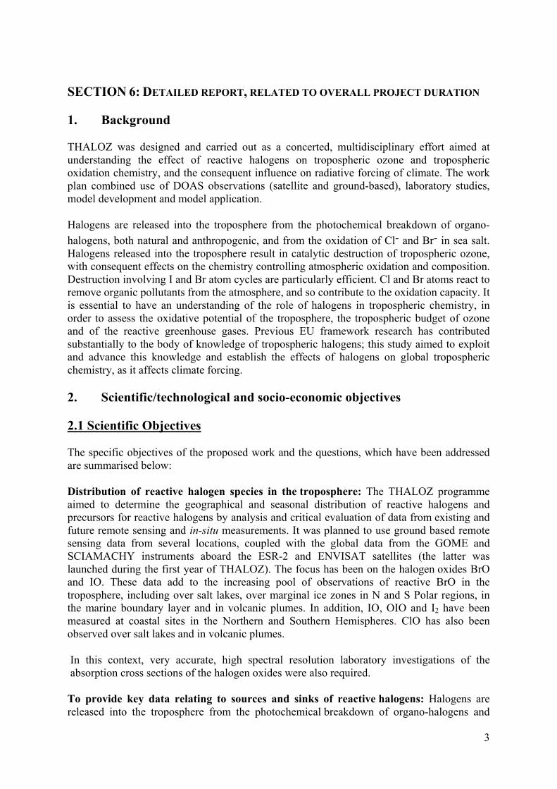
Method Two aspects of GOME data stability have been addressed within the project: the impact of variations in the measured irradiance and the effect of degradation of the scanning mirror. In the GOME instrument, solar irradiance measurements are performed via a diffuser plate, which is illuminated by the sun under slightly different angles throughout the year. These small changes result in variations of interference patterns from the diffuser surface, which in turn have an impact on the retrieved BrO column. To compensate for this problem, a normalisation technique was developed, which is based on the assumption of constant BrO columns over the equator (see Figure 3.1) and is now widely used in the community. A disadvantage of this technique is the introduction of a free parameter, which can only be determined by external information. As with any space-borne instrument, the external optics of GOME undergo degradation over their lifetime, and since the middle of 2001, changes in the GOME scanning mirror surface structure introduced spectral anomalies in the measurements depending on viewing direction. These anomalies correlate with BrO absorption structures and introduce a large scan angle dependency in the retrieved columns. Using the same assumption as for the irradiance correction, empirical compensation functions could be determined for each month, and a large improvement in consistency is achieved if these are included in the analysis (see Figure 3.2). With this approach, the GOME BrO time series could be extended from 2001 up to the present, albeit at reduced accuracy.

Results Analyses of nadir UV/visible measurements performed by GOME (or SCIAMACHY) provide total columns that include contributions from the stratosphere, the free troposphere and the boundary layer. For many applications, a separation of these three components is desirable, and one possible approach to such a separation has been evaluated within the project. The idea for this method is that stratospheric BrO is well represented in the 3D-CTM SLIMCAT and, therefore in combination with an appropriate airmass factor, can be used to correct the measurements for the stratospheric contributions. In Figure 3.3, an example is given for GOME measurements in March 1997. As can be seen, the boundary layer BrO

7

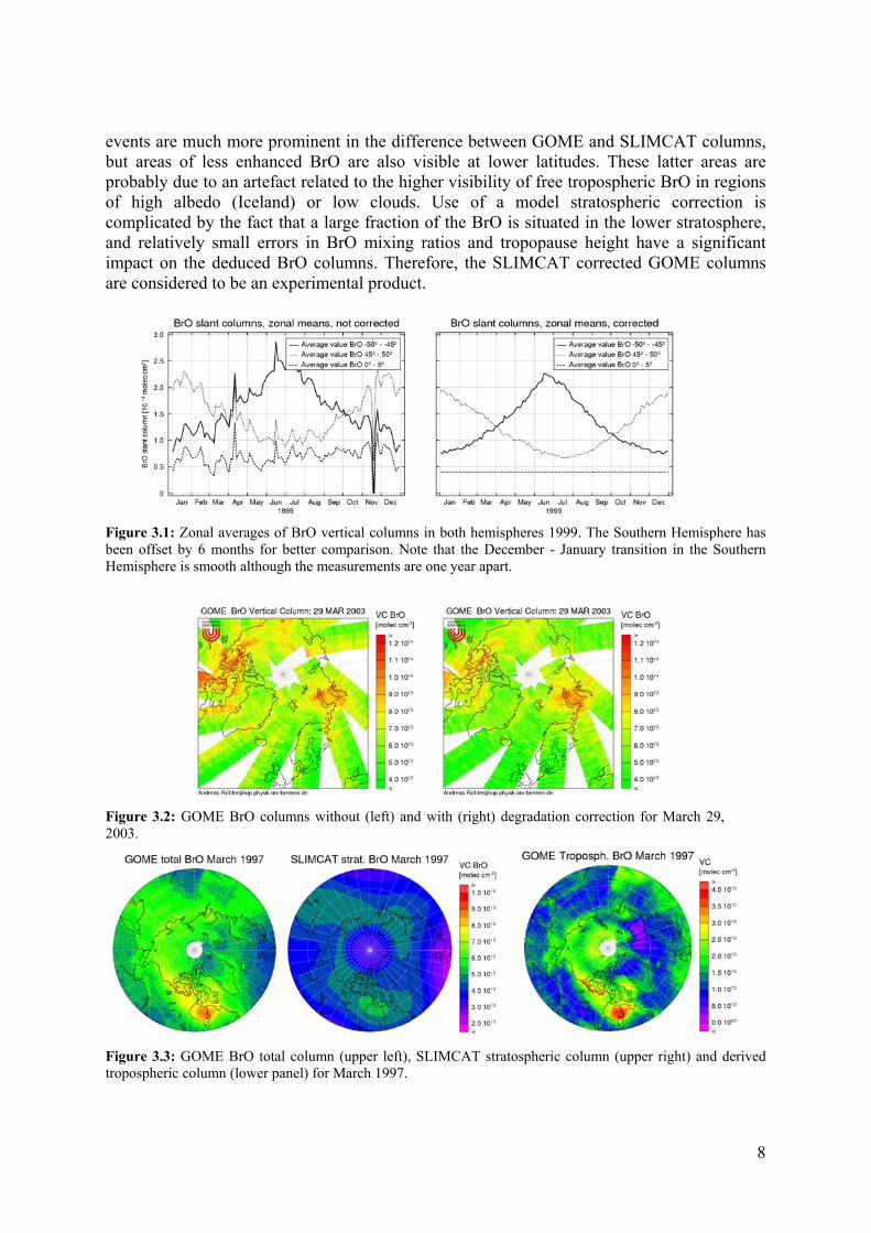
events are much more prominent in the difference between GOME and SLIMCAT columns, but areas of less enhanced BrO are also visible at lower latitudes. These latter areas are probably due to an artefact related to the higher visibility of free tropospheric BrO in regions of high albedo (Iceland) or low clouds. Use of a model stratospheric correction is complicated by the fact that a large fraction of the BrO is situated in the lower stratosphere, and relatively small errors in BrO mixing ratios and tropopause height have a significant impact on the deduced BrO columns. Therefore, the SLIMCAT corrected GOME columns are considered to be an experimental product.

Figure 3.1: Zonal averages of BrO vertical columns in both hemispheres 1999. The Southern Hemisphere has been offset by 6 months for better comparison. Note that the December - January transition in the Southern Hemisphere is smooth although the measurements are one year apart.

Figure 3.2: GOME BrO columns without (left) and with (right) degradation correction for March 29, 2003.

Figure 3.3: GOME BrO total column (upper left), SLIMCAT stratospheric column (upper right) and derived tropospheric column (lower panel) for March 1997.

8

3.1.2. SCIAMACHY Data Analysis

Background In March 2002, the Scanning Imaging Spectrometer for Atmospheric CHartography (SCIAMACHY) was launched, which is an improved version of the GOME instrument. With respect to the BrO retrieval, there are four main differences between the two instruments:

• The spatial resolution of SCIAMACHY is improved up to 30 × 60 km2 for BrO. • SCIAMACHY performs nadir and limb measurements, providing both the total

columns and stratospheric profiles respectively. • As limb and nadir measurements are alternating, the nadir coverage is reduced by a

factor of 2. • The time of overpass is 30 minutes earlier for SCIAMACHY, resulting in different

solar zenith angles (SZA), in particular at high latitudes in spring and autumn.

SCIAMACHY nadir measurements are available from August 2002 to present.

Method Important goals of the SCIAMACHY project are the continuation of the existing GOME time series, and the development of a BrO retrieval for SCIAMACHY. These were major aspects of the THALOZ project. As spectral coverage and resolution are very similar, the first approach was to apply GOME analysis settings to SCIAMACHY data after accounting for resolution differences. However, as a result of increased polarisation sensitivity of the instrument in the standard wavelength region of BrO retrieval, the results were unreliable and a UV-shifted wavelength window (336.0 – 347.0 nm) instead of 344.7 - 359 nm has to be applied. These analysis settings provide results that are consistent with GOME data (see Figure 3.4) with some still unresolved interferences from HCHO over tropical forests and a ‘ring effect’ over high mountains. To improve on the GOME situation, SCIAMACHY has a novel diffuser for solar irradiance measurements, and no normalisation over the tropics is needed. However, there is some impact of changes of Fraunhofer lines in the solar spectrum on SCIAMACHY BrO columns: daily solar measurements have to be used to avoid artefacts.

Results As pointed out above, the spatial resolution of SCIAMACHY is improved over that of GOME, and the effect of this was studied over both high latitudes and mid-latitude hot spots such as the Dead Sea and salt lakes in North America. Disappointingly, no clear signature of BrO could be found over the mid-latitude hot spots in spite of the improved resolution, which indicates that the high concentrations measured on the ground are probably restricted to a shallow layer on the surface and do not constitute a large vertical column. In contrast, the polar BrO events do show some fine structure in the SCIAMACHY data (Figure 3.5) but the overall pattern is very similar to that observed by GOME, indicating that the existing GOME time series is not biased too much by the poor GOME resolution.

SCIAMACHY limb measurements are timed to provide a stratospheric profile for nearly every nadir measurement. This can be used to create a stand-alone tropospheric BrO product without need for external data sets such as the SLIMCAT model output. As an example, GOME nadir and limb columns are shown in Figure 3.6. The general pattern of modelled and measured stratospheric columns is very similar, but SCIAMACHY profiles yield somewhat larger stratospheric columns in particular in the spring hemisphere in high latitudes. This

9

reduces the derived tropospheric BrO columns. Unfortunately, limb measurements of BrO are not very sensitive in the lower stratosphere, and a priori assumptions for this altitude contribute significantly to the retrieved BrO column. Therefore, more work is needed to evaluate the accuracy of this combined limb-nadir approach.

Figure 3.4: Comparison of SCIAMACHY (left) and GOME (right) BrO columns for April 2003. The agreement is good but not perfect; differences arise from a combination of differences in (1) spatial resolution, (2) spatial sampling and (3) the time of the overpass.

Figure 3.5: Comparison of two orbits of GOME (left) and SCIAMACHY (right) BrO columns over the Hudson Bay in March 2005. The improved spatial resolution results in higher local maxima in some areas but the overall pattern is the same.

Figure 3.6: Comparison of SCIAMACHY BrO columns from stratospheric limb measurements (left), from nadir measurements (middle) and SLIMCAT model columns (right, for 2000). The upper panel is for February, the lower for September.

10

3.1.3 Ground-based DOAS Measurements

Background Ground-based measurement of scattered sunlight is a well established technique to determine columns of molecular species having structured absorption spectra in the UV/visible wavelength range. These measurements have played a key role in the detection of halogen oxides (BrO and OClO) in the stratosphere. The instruments and analysis techniques used are very similar to those employed for satellite measurements from GOME and SCIAMACHY, and, in fact, ground-based DOAS instruments can be seen as precursors of the satellite instruments.

Method In a recent development, ground-based UV/vis instruments are no longer only observing the zenith-sky at twilight to optimise the measurement sensitivity in the stratosphere, but also make measurements at different angles close to the horizon. These “off-axis” measurements have very long light paths through the lower layers of the troposphere, and by combining a series of measurements at different elevation angles, limited profile information (2-5 layers) can be retrieved. In particular, the boundary layer, the free troposphere and the stratosphere can be separated. Given the structured spectra of several halogen compounds of atmospheric relevance (e.g. BrO, IO, OIO, OClO, I2); these instruments are powerful tools to study atmospheric abundances of halogen compounds over longer periods of time.

Within the THALOZ project, data from several ground-based DOAS instruments operated by the University of Bremen (Figure 3.7) have been analysed for signatures of tropospheric BrO and IO. In addition, a travelling instrument has been installed for several months in List on Sylt, North Frisian Island: 55.02°N, 8.43°E directly viewing the tidal zone. The first step was to develop the necessary tools to understand the radiative transfer for this novel observation geometry, and to develop appropriate retrieval methods.

In Ny-Alesund, enhanced BrO is observed sporadigeometry, it is obvious that this BrO is located in tBrO columns are shown in Figure 3.8 for April observed during snow fall, and as a result of multviewing directions showed similar values. On thprevailed and the horizon viewing directions recozenith viewing direction, indicating that about 4 - 5layer. These events of high BrO coincide with strolinked to depletion in total gaseous mercury (TGMbetween the natural bromine explosions and anthrinput into the Arctic environment.

Figure 3.7: Stations of the University of Bremen Network of ground-based UV/vis DOAS instruments (BREDOM)

cally, and with the new off-axis viewing he lower boundary layer. As an example, 20, 2002. A large increase of BrO was iple scattering under these conditions, all e following days, clear sky conditions rded a much larger BrO signal than the ppt of BrO were present in the boundary ngly depleted surface ozone, and are also

), Figure 3.9. This is an important link opogenic pollution, in this case mercury

11

0

1

2

3

4

5

6

20.04.2002 22.04.2002 24.04.2002 26.04.200260

70

80

90

-4

-2

0

2

4

6

8

10

Slan

t col

umn

BrO

[1

014 m

olec

/cm

2 ]

Zenith3°

SZA

[°]

Sla

nt c

olum

n O

4

Figure 3.8: Ground-based BrO measurements in Ny-Ålesund in April 2002. Upper panel: BrO columns for zenith (black) and horizon view (red). Middle panel: O4 columns as an indicator for clouds, smooth variations and large differences between the viewing directions indicating clear sky. A large enhancement in BrO could be observed from April 20 to 21 during snow fall and values decreased over the next days back to normal.

Figure 3.9: Surface layer ozone (1-h average) and TGM (12 samples h−1) and Zenith slant columns of BrO sampled over Ny- Alesund together with indexed (integrated 6-h average) sea-ice transect of 72-h backward trajectories ending at Ny-Alesund 6, 12, 18 and 24UTC. Figure from Sommar et al., 2004.

Closer analysis of the Ny-Alesund data and measurements from other stations show, that there also seems to be a tropospheric background of about 1 ppt of BrO at higher latitudes, in agreement with estimates based on satellite and balloon data. However, the quantification of this BrO background is still difficult.

Analysis of the measurements in List show repeated evidence for IO in the range of 1ppt (Figure 3.10), but no correlation with the tides could be established. Similar concentrations of IO were also observed on Ny-Alesund. Whilst IO seems to be present in coastal regions of the North Sea, concentrations are not everywhere as large as observed in Mace Head.

Figure 3.10: IO slant columns (left) and O4 slant columns (right) for measurements on a clear day in List (01.06.2004). Enhanced IO of about 1 ppt in the lower troposphere could be detected on this and several other days.

12

3.2 Reactive Halogen Source Terms

3.2.1 Organic Halogen Source Terms

3.2.1.1 Bromocarbons

Introduction Bromocarbons, generated in the ocean by marine organisms, are an important source of atmospheric bromine. However, global ocean-to-atmosphere fluxes of bromocarbons are highly uncertain due to large spatial and temporal variations in the geographical distribution of the marine organisms that generate them, and the gas-exchange coefficient between the ocean and the atmosphere (which will vary with wind speed). Bromoform (CHBr3) provides the largest contribution to tropospheric reactive bromine of all the oceanic bromocarbons due to its large flux to the atmosphere, short lifetime and high bromine content. Estimates of global CHBr3 emissions from the ocean cover a wide range from ~200 to over 1000 Gg CHBr3/yr (e.g. [WMO, 1999]; [Penkett et al., 1985]; [Carpenter and Liss, 2000]). Methyl bromide (CH3Br), which has both natural (oceanic and terrestrial) and anthropogenic emissions has also been studied, within this project, to identify and evaluate possible candidates for the ‘missing’ surface source, identified in earlier studies [Lee-Taylor et al. 1998] and required to balance its atmospheric budget. Methyl bromide is the most abundant species containing bromine in the free troposphere and one of the largest carriers of bromine to the lower stratosphere ([Schauffler et al., 1993]; [Kourtidis et al., 1998]; [Cicerone et al., 1988]; [Dvortsov et al., 1999]).

Method Model integrations in this study have been performed using the global 3D chemical transport model, TOMCAT. This model has been used extensively for tropospheric studies. Details about the model and its validation against data can be found in: Law et al. [1998], Stockwell et al. [1998], and Wang et al. [1999]. The version of TOMCAT used in this work has been modified to include a simple chemistry scheme consisting of ‘coloured’ methyl bromide tracers and prescribed OH fields and photolysis frequencies. The prescribed sink fields significantly decrease the amount of computer time required, compared to ‘full chemistry’ model integrations, and were used successfully in a model study of tropospheric methane [Warwick et al., 2002].

In two separate studies ([Warwick et al 2005a] and [Warwick et al., 2005b]) a variety of prescribed emission scenarios have been used to simulate atmospheric concentrations of CH3Br and oceanic sources of CHBr3. Comparison of simulated and measured values provides an indication of the likely surface to atmosphere flux. Further simulations have been carried out for oceanic sources of the other major short-lived bromocarbons (CH2Br2, CH2BrCl, CHBr2Cl, CHBrCl2 and CH3Br) to provide an estimate of the amount of reactive bromine, released from these compounds, in the troposphere and lower stratosphere.

Results The first study to be carried out within this area was designed to investigate the ‘missing’ methyl bromide source identified by Lee-Taylor et al. [1998]. One base-line emission scenario and five further plausible scenarios were considered. The additional emission scenarios were specifically designed to test whether the geographical distribution and seasonal cycles of additional vegetation and/or increased biomass burning emissions are

13

consistent with atmospheric observations of methyl bromide mixing ratios. Both the inclusion of a vegetation source in the tropics, leading to a significantly larger vegetation source than that described in WMO [2003], and a double strength biomass burning source substantially improve the agreement between model simulations and atmospheric measurements compared with the base-line emission scenario. Small differences between the simulated seasonal cycles of different emission scenarios makes it difficult to distinguish between the relative likelihoods of model scenarios containing a tropical vegetation source or an increased biomass burning source.

To assess the extent to which observed atmospheric concentrations of bromocarbons can constrain the ocean-to-atmosphere flux, information from previous published studies concerning the possible source distributions were gathered and used to create several prescribed emission datasets which could be tested in atmospheric model simulations. For bromoform, global emission datasets tested in the model included, initially, (1) a spatially uniform oceanic source [WMO, 1999], (2) a latitudinally varying open ocean source [Quack and Wallis, 2003] and (3) a coastline only source [Quack and Wallis, 2003]. These emission scenarios all failed to reproduce the observed distribution of bromoform seen in atmospheric measurements [Schauffler et al., 1998]. Further emission scenarios with alternative geographical distributions (including strong emissions in the tropics) were therefore created in an attempt to improve the comparison between modelled and observed latitudinal variations and vertical profiles of bromoform mixing ratios, see Bromine Budget, Section 3.4.

Two of the emission datasets described in the model were better able to capture the observed bromoform distribution. The first is considered to be at the lower end of the emission estimates, as it contains no coastline emissions and modelled mixing ratios are on average lower than observations. The second, which has a 50% larger global annual emission of bromoform, due to strong coastal emissions, gives a high estimate for annual global bromoform oceanic emissions. If this later emission dataset is increased significantly, modelled free tropospheric values would exceed observations in the Pacific region. These two scenarios (‘low’ CHBr3 scenario and ’high’ CHBr3 scenario) were combined with a single open-ocean, prescribed emission dataset for other short-lived oceanic bomocarbons (CH2Br2, CH2BrCl, CHBr2Cl, CHBrCl2) and an emission dataset for methyl bromide, from Warwick et al. [2005a]. A comparison of the two scenarios with measurements is shown in Figure 3.11. The model is able to reproduce total organic bromine to a satisfactory level in both scenarios. It should be noted that a higher flux of all bromocarbons, than that recommended by WMO [1999], is required to reproduce measurements, see Table 3.1.

Bromocarbon Emitted

Low CHBr3 Scenario

High CHBr3 Scenario

Global Flux, from WMO 1999, (Gg/yr)

CHBr3 400 595 207 CH2Br2 113 113 58 CH2BrCl 6.8 6.8 4.7 CHBr2Cl 23 23 16 CHBrCl2 16 16 11 CH3Br 131 131 122 Table 3.1: Model simulations of bromocarbon global flux compared with recommendations by WMO.

14

In summary, our model simulations indicate that emissions of bromoform to the atmosphere are likely to be 400 – 600 Gg/yr, depending upon the geographical distribution of emissions, and, as coastal emissions are likely to be important, [Quack and Wallis, 2003], we expect emission estimates to be at the higher end of this range. This is considerably higher than that recommended by WMO (210 Gg/yr). Fluxes of all other bromocarbons are also higher than that recommended by WMO. The source distribution of methyl bromide has also been rigorously studied, leading to a conclusion that there is an additional source in the tropics, which could be due to either an increased vegetation or biomass burning source.

Figure 3.11: Tropospheric average latitudinal distributions of total organic bromine from the short-lived oceanic bromocarbons (solid red line) and, in addition, from methyl bromide (solid black line) from averaged PEM tropics samples in the Pacific region. The open and solid circles show tropospheric average modelled total organic bromine in the central pacific for the short-lived oceanic bromocarbons only and the short-lived bromocarbons and methyl bromide, respectively.

3.2.1.2 The Chemistry of Organo-halogens in Seawater and their Flux to the Atmosphere

Method Solutions of dihalomethanes (CH2I2, CH2ClI and CH2BrI) in seawater have been investigated in order to determine which reactions are important in the surface and mixed layers of the ocean. Nucleophilic substitution of CH2I2 and photolysis reactions of CH2I2, CH2ClI and CH2BrI have been investigated by placing, as appropriate, the solutions in the dark or irradiating over the full solar spectrum, using a Xe lamp equipped with air-mass optical filters. In addition the wavelength dependence of the photolysis of CH2I2 solutions has been investigated. In a further experiment the reaction of HOI / I2 with organics, naturally present in seawater has also been investigated.

Analysis of solutions has been carried out by Gas Chromatography for halocarbons and by voltammetry for iodide. All experiments have been carried out with sterilized solutions.

15

Hence, only abiotic reactions should occur. For experimental details see the THALOZ annual reports.

Nucleophilic substitution reactions Results indicate that CH2I2 does not undergo nucleophilic substitution, by chloride or bromide ions in artificial seawater, at 15 °C or at 30 °C, at least within the timescale of the experiment (one week).

CH2I2, CH2ClI and CH2BrI photolysis Results from the photolysis of all the dihalomethanes in different water types are summarised in Table 3.2. Most irradiations were carried out at 5600 Wm-2 (to give a rapid degradation of the dihalomethane standards). The values given in Table 3.2 were extrapolated to 1100 Wm-2, as the photolysis rate was observed to be proportional to the radiant flux. All compounds were found, at least initially to follow first-order removal kinetics. However, for CH2I2, deviations from first-order kinetics occurred after a few minutes of irradiation, probably indicating recombination of the CH2I and I radicals. The photo-degradation of CH2I2 was similar in all water types (Figure 3.12), suggesting that direct photolysis occurs and not reaction with other products of photolysis, which might be present in real seawater. Photolysis of CH2I2 generated CH2ClI with a yield variable between 25 and 50%. Photolysis of CH2ClI was approximately 60 times slower than that of CH2I2, with production of CH2Cl2. Photolytic loss of CH2BrI occurred over timescales intermediate between those of CH2ClI and CH2I2, and formation of CH2ClBr was observed, with a yield of about 5%. As expected from the investigation of nucleophilic reactions, no degradation was observed to occur in the dark, for any of the dihalomethanes.

Table 3.2: Photolysis rates (k) and photolytic lifetimes (τ) for dihalomethanes at 1100 Wm-2.

Compound Water type

k / s-1 τ

CH2I2 MQ (1.3 ± 0.1) ×10-3 13 ± 1 min ASW (1.4 ± 0.1) ×10-3 12 ± 1 min NORW (1.4 ± 0.2) ×10-3 12 ± 2 min UKCOAST (1.1 ± 0.2) ×10-3 15 ± 2 min CH2ClI ASW (2.6 ± 0.1) ×10-5 10.6 ± 0.3 h NORW (2.1 ± 0.1) ×10-5 13.5 ± 0.6 h CH2BrI ASW (5.8 ± 0.2) ×10-5 4.8 ± 0.1 h NORW (5.7 ± 0.1) ×10-5 4.7 ± 0.1 h

MQ: Milli-Q water (18 MΩ); ASW: Artificial seawater; NORW: Norwegian seawater (75°N, 15°E); UKCOAST: Coastal water (Lowestoft, U.K.)

0

10

20

30

40

0 250 500 750 1000Time /s

CH 2

I 2 /

pM

.

MQASWUKCOASTNorw

Figure 3.12: Variation in CH2I2 concentration as function of irradiation time in different water types at 5600 Wm2. Legend as in Table 3.2.

CH2I2 quantum yields The absolute quantum yields (Φλ) for CH2I2 photodegradation in natural seawater were determined at 10 and 15 nm bandwidths. The values of the absolute quantum yield that were obtained are shown in Table 3.3. These values were used to calculate the overall rate constant for CH2I2 photolysis at any water depth, according to the following equation:

16

k (s-1) = 2.303 Σλ Φλ Iλ ελ

where Iλ is the solar irradiance (molecule photons cm-2 s-1) and ελ is the molar extinction coefficient at wavelength λ (mol dm3 cm-1). The rate constant value calculated for the sea surface at the equator (with overhead sun) was 1.5×10-3(±10-4) s-1, which agrees very well with the value of 1.4×10-3(±10-4) s-1 measured from full-spectrum irradiations at 1100 Wm-2. Calculation of sunlight-normalised photolysis rates show that the photolysis of CH2I2 occurs predominantly between 300 and 350 nm, with a maximum at 320 nm (Figure 3.13b).

The NASA COART (Coupled Ocean and Atmosphere Radiative Transfer) model was used to calculate the solar irradiance at the sea surface and its attenuation with depth in the water. These data were used to calculate photolysis rates as a function of depth in different oceanic water types (Figure 3.14). Although wavelengths in the UV part of the solar spectrum are quickly attenuated with increasing depth in oceanic waters, photolysis of CH2I2 still occurs as deep as 40 m in the clearest waters.

Table 3.3: Absolute quantum yield values for CH2I2.

Wavelength / nm Bandwidth / nm Φ (actinometry) Φ (power meter) 290 10 0.37 ± 0.02 0.35 ± 0.02 300 10 0.39 ± 0.02 0.40 ± 0.02 310 10 0.38 ± 0.01 0.38 ± 0.02
320 10 0.34 ± 0.01 0.35 ± 0.02
330 10 0 3 ± 0.02 0.34 ± 0.02 340 10 0 3 ± 0.02 0.34 ± 0.02 3 0 10 0 2 ± 0.02 0.27 ± 0.03 365 15 0 3 ± 0.13 0.39 ± 0.05 0.

0.

0.

0.

Pho

toly

sis

rate

/ pM

µE

0

1

2

3

4

Sunl

otol

ysig

htis

ra-n

orte

/ pm

ali

M c. 1

. 35 . 7

. 4

A

00

04

08

12

0.16

0.20

280 300 320 340 360 380

Wavelength / nm

-1

B

5

6

280 300 320 340 360 380

Wavelength / nm

sed

ph

m -2

day

-1

Figure 3.13: (A) Rate of photolysis of CH2I2 per unit energy absorbed as function of wavelength. The photolysis rates were calculated assuming an initial CH2I2 concentration of 0.5 pM. (B) Photolysis rates normalised to the average summer solar irradiance averaged over 10 and 15 nm bandwidths.

0

10

20

30

40

50

60

0.0 0.2 0.4 0.6 0.8 1.0

k / s-1

dept

h / m

50°N, chla 1.5 mg/m330°N, chla 0.05 mg/m3Equator, chla 0.2 mg/m3

Figure 3.14: Fractional photolysis rate of CH2I2 in different types of oceanic seawater.

17

Mixed layer model The results of the photolysis study have been used to develop a box model for CH2I2 and CH2ClI in a shallow (50-80m) equatorial mixed layer, which includes air-sea exchange and photochemical transformation of both species. Field measurements [Chuck, 2002] were used to predict the necessary biological production rates that would support the observed fluxes (0-15 nmol m-2 day-1; average 6 nmol m-2 day-1) to the atmosphere in equatorial waters, assuming that the only loss processes are photochemical degradation and sea-to-air transfer. All model runs have assumed that CH2I2 production occurs at 40-50 m depth, collocated with the chlorophyll maximum, just above the thermocline [Yamamoto et al., 2001]. In this model, all CH2ClI derives from the photodegradation of CH2I2 with a 50% yield. Atmospheric concentrations of CH2I2 and CH2ClI used for flux calculations are, respectively, zero and 0.04 pptv at the equator [Chuck, 2002]. Photolysis rates of CH2I2 at each depth were calculated as detailed in the previous section. Quantum yield values for CH2ClI are unknown. However a comparison of the absorption cross sections suggest that photolysis rates for CH2ClI may be attenuated faster than those of CH2I2 with increasing water depth. The model has therefore been run under two “extreme” scenarios: (i) photolysis rates for CH2ClI following the same attenuation with depth than those for CH2I2; and (ii) photolysis of CH2ClI occurring in the top 1 m of the water column only.

In order to support a flux of 6 nmol m-2 day-1 [Chuck, 2002], the model requires a CH2I2 production of 0.06-0.2 nmol m-3 h-1 (depending on the extent of CH2ClI photolysis. Results in Figure 3.15 show depth profiles for CH2I2 and CH2ClI under the two different scenarios. Concentration of CH2I2 is highest at depth and gradually decreases towards the sea surface, due to photolysis and venting to the atmosphere; sea-surface concentrations are very low in both scenarios (<0.1 pmol L-1, near to or below detection), as a consequence of the fast photolysis rate of CH2I2, and result in an average sea-to-air flux of 0.1-0.2 nmol m-2 day-1. CH2ClI is photodegraded at a slower rate than CH2I2 and, therefore, higher concentrations occur through the water column under both photodegradation scenarios; in both cases, the sea surface concentration (~2.7 pmol L-1) would be detectable. For the highest CH2ClI flux value of 15 nmol m-2 day-1, calculated by Chuck [2002], the model requires a CH2I2 production rate varying between 0.15 nmol m-3 h-1 (assuming CH2ClI photolysis at the sea surface only) and 0.5 nmol m-3 h-1 (assuming CH2ClI photolysis occurs through the water column).

Figure 3.15: Simulated depth profiles for CH2I2 (blue diamonds) and CH2ClI (red squares) supporting a CH2ClI sea-air flux of 6 nmol m-2 day-1: (A) CH2I2 production rate of 0.2 nmol m-3 h-1 and CH2ClI photolysis occurring through the water column with same depth-dependency as that of CH2I2; (B) CH2I2 production rate of 0.06 nmol m-3 h-1 and photolysis of CH2ClI occurring in the top 1 m box only.

0

20

40

60

0 1 2 3 4

concentration / pmol L-1

dept

h / m

A

0

20

40

60

0 1 2 3

concentration / pmol L-1

dept

h / m

B

4

Reaction of HOI with natural organic matter in seawater

18

A poorly investigated pathway for the production of organo-halogens is the reaction of inorganic species with dissolved organic matter (DOM) in seawater. The reaction of I2 or HOI, through the hydrolysis of I2, has been investigated in seawater, and in sterile solutions containing DOM from the incubation medium of the macroalga Enteromorpha Intestinalis.

Addition of I2 to Norwegian Sea seawater and North Sea seawater, to form a solution 0.063 µM in I2, resulted in production of CH2I2 and traces of CH3I. A wider range of iodocarbons were formed when I2 was added to the incubation medium of the macroalga Enteromorpha Intestinalis. Different iodocarbons were generated at different rates. The formation rate of CH3I and most poly-iodinated compounds was an order of magnitude higher than that of the iodopropanes, CH2ClI and CH2BrI; the formation rate of CH2I2 was two orders of magnitude higher.

The emission of iodocarbons from the incubation medium of the macroalga Enteromorpha Intestinalis was compared with emission of iodinated compounds from live macroalgae. Whilst macroalgae emitted much higher concentrations of brominated than iodinated compounds (results not shown), nearly all the monitored iodocarbons were produced, Figure 3.16. Addition of I2 to the incubation medium resulted in the production of only CH2I2, CH2BrI and CHBr2I, while addition of I2 to the controls resulted in the production of CH2I2 and CH3I.

0 50 100 150 200 250 300 350 400

CH3I

C2H5I

CH3CHICH3

CH2ClI

CH2BrI

CHClBrI

CH2I2

CHBr2I

pM compound

HOI + controlsHOI + algal mediumalgae/ g wet weight

Figure 3.16: Emissions of iodocarbons by Enteromorpha Intestinalis (blue), and variation in iodocarbon concentration after the addition of 0.15 µM I2 to the algae incubation medium (red) and to the controls (yellow).

In summary, photochemical reactions of iodocarbons do occur in seawater; whereas nucleophilic substitution reactions do not occur on timescales relevant to the ocean surface and mixed layers. This is the first study to show that photolysis of CH2I2 in seawater does occur, producing CH2ClI directly, with no need for organic photosensitisers. The yield in CH2ClI varies between 25 and 50%, and it has been shown that iodide is also produced. The results of the laboratory work suggest that CH2I2 is quickly photolysed (τ = 10s of minutes near the surface in full sun) in the water column and is depleted at the sea surface; whereas CH2ClI, having a longer photolytic lifetime (τ = 10s of hours near the surface in full sun), can escape to the atmosphere. These results are in good agreement with atmospheric measurements which show that, of the two compounds, only CH2ClI has been detected in the oceanic atmosphere.

Work on the reaction of I2 (or HOI, via hydrolysis) in seawater shows that organo-iodides are produced. The magnitude and type of organo-iodides produced depends upon the organic matter present. Formation of a wider range of iodocarbons occurs in the presence of fresh biogenically produced organic matter.

19

3.2.2 Inorganic Halogen Source Term

3.2.2.1 Halogen Chemistry Survey

A survey of halogen chemistry in the marine boundary layer (MBL) was written and published [Adams and Cox, 2002]. In the article particular emphasis was placed on the influence of the halogens on ozone and oxidising processes. The sources, sinks and cycling of reactive halogen species in the MBL were discussed and differences in the reactivity of gas phase chlorine, bromine and iodine species highlighted. A brief description of the properties of marine aerosols was given, including the physical and chemical nature of both freshly generated and chemically “aged” sea salt particles. Heterogeneous reactions on these particles were surveyed and chemical mechanisms of halogen release, including acid displacement, NOx redox reactions and reactions of hypohalous acids assessed. The impact of halogen chemistry on ozone and oxidation of VOCs was described.

3.2.2.2 Heterogeneous Reaction Kinetics

Method A Knudsen cell interfaced to a mass spectrometer was used to study the uptake and reaction of HOCl (and Cl2O) on frozen salt solutions. HOCl was generated by hydrolysis of Cl2O. However, as these two species are in rapid equilibrium there was always residual Cl2O (~20%). For this reason two parallel kinetic investigations had to be performed: one with pure Cl2O, and the other with the mixture HOCl + Cl2O. The presence of Cl2O did not affect the uptake coefficient of HOCl. However, the product distributions were altered. The frozen substrate was prepared by slowly freezing a sea salt (“sel de Guérande”) or KCl solution within the Knudsen cell. No difference was seen if NaCl was used as the frozen substrate. Different fluxes were obtained by varying the aperture size. The highest flux of ~1×1015 molecule s-1 corresponds to ~4×1010 molecule cm-3, which is equivalent to 1.5 ppb at 1 bar. The calibration of the MS signals of HOCl at m/e 5153 and of Cl2O at m/e 52/54 or 86/88/90 in terms of absolute concentrations in the reactor has been described in previous reports.

An aerosol flow reactor coupled to a mass specrometer was used to study the uptake and reaction of HNO3, HOCl and HOBr on aerosol generated from salt solutions, including genuine sea salt solutions. The flow rates were chosen so as to afford gas phase residence times in the range 15 to 90s coupled to aerosol conditioning times of 15s. The HOBr source was set up by flowing an air stream across a trap containing Br2 at ambient temperature, which reacted in a 30cm long and 9mm ID glass tube with yellow HgO powder loosely deposited at the bottom of the source tube. HOBr concentrations of the order of < 3×1013 molecule cm-3 have been obtained.

The interactions of reactive halogen species with seawater and model seawater have been studied using a wetted wall flow tube - mass spectrometer system. A slowly flowing film of liquid is formed on the inside wall of a vertical, cylindrical reactor. Trace gas species are introduced into the reactor via a movable injector. The gas-liquid contact time is known and may be varied. Both the reactive species and any gas phase products are detected.

20

An aerosol flow tube – CIMS system (AFT-CIMS) has been developed to perform uptake experiments (Figure 3.17). Aerosol is generated and the relative humidity (RH), thus aerosol

phase, controlled. The surface area of aerosol is measured using a DMA, (Hauke EMS-08). The reactive species is introduced via a moveable injector. Uptake and production of volatile species are observed using the CIMS. The CIMS was tested with both SF6

- and O2- reagent ions and SF6

- selected. The detection limit for ICl is 50 ppb. Due to significant decreases in sensitivity with gas phase water content, high RH experiments were performed at 274K. Tandem DMA (TDMA) experiments were performed to measure the growth of aerosol particles (for aerosol size correction in the low temperature experiments). See Appendix 2.4.

Figure 3.17: Schematic of the AFT-CIMS

Results Heterogeneous reactions of HOCl on frozen salt surfaces Reference experiments on the interaction of HOCl and Cl2O on pure ice at 200K have been performed using a 4 mm aperture reactor. At a medium flow rate of HOCl of FHOCl = (5.0 ± 1.5)×1014 molecule s-1 a steady state uptake coefficient γss = (5.5 ± 0.4)×10-4 was measured once the more rapid initial uptake of HOCl, lasting for ca. 150 s, had subsided. As expected, no Cl2 formation was observed. The corresponding Cl2O rate of uptake resulted in γss = (2.8 ± 0.7)×10-4 at FCl2O = (2.4 ± 0.6)×1014 molecule s-1, again after a rapid initial burst of uptake lasting approximately 20s. Although the γ values decreased somewhat with increasing concentration of both HOCl and Cl2O it was nevertheless found convenient to express the uptake kinetics in terms of a first order rate law. The slow but sustained uptake of Cl2O on ice at 200K is accompanied by slow formation of Cl2 and HOCl at 200K, potentially according to the following reactions:

Cl2O + ice → Cl2 + 0.5O2 (1) Cl2O + H2O(ice) → 2HOCl (2)

It is likely that in reaction (2) one molecule of HOCl remains on the ice whereas the other molecule is released into the gas phase in analogy to the interaction of Cl2O on solid alkali halide salts. Figure 3.18 displays representative examples of HOCl and Cl2O uptake on frozen KCl and sea salt solutions and Table 3.4 displays the corresponding kinetic results for the initial uptake of Cl2O and HOCl, as well as the product yields for the formal reactions (3) and (4) on frozen sea salt and KCl solution:

HOCl + NaCl → Cl2 + NaOH (3) Cl2O + NaCl → Cl2 + NaOCl (4)

21

New Sample frozen solution KCl Sea Salt HOCl Slow for pure Cl2O uptake None for pure Cl2O uptake Product

Formation Cl2 Transient for HOCl uptake and for pure

Cl2O uptake Fast for HOCl and pure Cl2O uptake

Escape orifice (mm) 4 14 4 14 HOCl (Cl2O)0 HOCl (Cl2O)SS (Cl2O)0 (Cl2O)SS

(1.2 ± 0.5) × 10-2 (2.8 ± 1.3) × 10-3 (3.0 ± 1.1) × 10-2 (4.6 ± 0.8) × 10-4

(8.3 ± 2.5) × 10-2 (2.5 ± 0.7) × 10-2 (1.8 ± 0.6) × 10-1 (1.1 ± 0.3) × 10-1

(1.6 ± 0.5 ) × 10-2 (2.5 ± 0.7) × 10-3 (1.6 ± 0.6) × 10-2 (1.8 ± 0.9) × 10-2

(5.4 ± 1.6) ×10-2 (2.6 ± 0.8) × 10-2 (1.8± 0.4) ×10-1 (1.6 ± 0.6) × 10-1

γ Mixture of HOCl and Cl2O Pure Cl2O

Cl2O0 Cl2OSS

(4.5 ± 1.4) × 10-2

(4.7 ± 1.2) × 10-3 (2.8 ± 1.1 ) × 10-1 (1.4 ± 0.5) × 10-1

(3.3 ± 1.4) × 10-2 (2.8 ± 0.8) × 10-3

(2.5 ± 0.7) × 10-1 (2.3 ± 0.6) × 10-1

Table 3.4: Uptake coefficient γ for uptake of HOCl and Cl2O on fresh KCl and sea salt frozen solutions at 200K and at FHOCl = (5.0 ± 1) × 1014 and FCl2O = (2.0± 0.5) × 10 14 molecule s-1.

b) Cl2O on sea salt: FCl2O = (1.9 ± 0.5) × 1014 -1

a) Cl2O on KCl: FCl2O = (1.7 ± 0.4) × 1014 molecule s-1

V

)

MS

(

0.25

0.20

0.15

0.10

0.05

0.00

6004000

reaction ON

200time (s)c) HOCl on KCl: FHOCl = (7.6 ± 0.8) × 1014 molecule s-1

FCl2O = (1.9 ± 0.5) × 1014 molecule s-1

0.30

0.25

0.20

0.15

0.10

0.05

0.00

MS

(V)

10008006004002000

reaction ON

molecule s

time (s)d) HOCl on sea salt: FHOCl = (9.0 ± 0.3) × 1014 molecule s-1 FCl2O = (2.1 ± 0.5) × 1014 molecule s-1

0.5

0.4

0.3

0.2

0.1

0.0

MS

(V)

8006004002000time (s)

reaction ON 0.5

0.4

0.3

0.2

0.1

0.0

MS

(V)

8006004002000 time (s)

reaction ON

Figure 3.18: Typical Cl2O and HOCl experiment on fresh KCl and frozen sea salt solution using a 4 mm aperture Knudsen cell. The change in the mass spectrometer response to Cl2O (Blue), HOCl (Black) and Cl2 (Yellow) is shown as a function of exposure time.

At comparable flow rates, i.e. concentrations, γCl2O for pure Cl2O and γCl2O for the mixture of Cl2O and HOCl are the same within experimental uncertainty except for the KCl results, obtained in the 4 mm diameter aperture reactor, as displayed in Table 3.4. This supports our assertion that the simultaneous interactions of Cl2O and HOCl with frozen salt surfaces are independent of each other. As noted above, both γ0 and γss decrease with increasing concentration. The uptake coefficient for Cl2O on both frozen KCl and sea salt is larger than for HOCl. The uptake of Cl2O can therefore not be neglected as far as Cl2 formation is

22

concerned. The uptake coefficients for each species are the same for the two different substrates within experimental uncertainty. In contrast, the rate of formation of Cl2 differs between frozen KCl and frozen salt solution. Whereas it is transient on KCl on a time scale of approximately 200s, it seems sustained on frozen sea salt solution. This may be due to the internal buffering capacity of sea salt vs. KCl frozen solution discussed below, that neutralizes the basicity generated in reactions (3) and (4). In contrast to frozen KCl solution where the rate of HOCl formation is significant after an induction time of approximately 200s, formation of HOCl from Cl2O seems to be suppressed on frozen sea salt solutions.

Despite a sizable uptake of both HOCl and Cl2O when using the reactor with a 14 mm aperture (see Table 3.4), no additional Cl2 formation, due to the interaction of HOCl with frozen sea salt and KCl solution, has been observed. This is in contrast to the 4 mm orifice reactor (Figure 3.18) where additional Cl2 formation has been measured owing to the presence of HOCl. The smaller surface coverage in the 14 mm vs. the 4 mm orifice reactor apparently precludes the formation of Cl2. For the same reason, there is no additional Cl2 formation from both HOCl and Cl2O uptake in the 4 mm aperture reactor at 215K, compared to the interaction of pure Cl2O.

The yield of Cl2 produced per Cl2O molecule taken up can be calculated from experiments where only Cl2O was present. By subtracting the contribution from Cl2O, when a mixture of HOCl and Cl2O was used, the yield of Cl2 per HOCl molecule taken up can be derived. This approach assumes that the kinetics of Cl2O uptake and reaction are unaffected by the presence of HOCl and leads to a value of 0.30 ± 0.10 and 0.23 ± 0.10 for KCl and sea salt solution, respectively. The fate of the excess HOCl taken up is uncertain, but potentially it will remain in the ice substrate at T = 200K and may remain available for the oxidation of other deposited atmospheric species, such as elemental Hg. The reactivity of the chloride/ice surfaces could be increased by adding a buffer.

Similar kinetic results have been obtained for frozen KCl and sea salt samples that had been contaminated by previous exposure to HOCl and/or Cl2O. However, although Cl2O uptake decreased to zero during the repeat experiment on a frozen KCl solution, Cl2 formation continued, albeit only at a small rate. This Cl2 is a product of HOCl uptake and formation stops upon halting the HOCl flow into the reactor. Analysing the calibrated signals once Cl2O uptake ceases gives a yield of Cl2 of 0.3 (per HOCl taken up), which is the same as the value determined above.

Experiments were also performed at 215 K. In this case, the measured values for γ0 and γss of HOCl are smaller than for 200K. Conversely, γ0 and γss for Cl2O are significantly larger at 215K, especially for frozen KCl solution. However, the results at 215K are marked by the complete absence of additional Cl2 formation owing to specific HOCl/frozen salt interaction, despite significant uptake of both HOCl and Cl2O. The uptake of both HOCl and Cl2O appears complex as an increase in temperature leads to a decrease of the reaction product Cl2. This also means that 70% of the HOCl taken up has not yet reacted to Cl2 at 200K and is stored as a species other than Cl2 trapped in the ice matrix.

Huff and Abbatt [2000] determined an upper limit value of γ < 4.5×10-3 at 233K using a coated-wall flow tube reactor coupled to a mass spectrometer, which is essentially consistent with the present results if extrapolated from 215 to 233K. These workers did not observe any uptake of HOCl on a frozen NaCl salt surface whose concentration was in the range 0.1 to

23

1% by weight. In comparison, the present salt concentration was 3.5% by weight for NaCl and sea salt. However, we would like to stress that the surface concentration of the salt atop the ice matrix is unknown.

Heterogeneous reaction of HNO3 with NaCl and sea salt aerosol An atmospheric aerosol flow tube coupled to electron-impact mass spectrometry and aerosol metrology has been commissioned in order to conduct heterogeneous chemical kinetic studies on salt aerosols. Reaction (5) was chosen as it is has been studied previously and can therefore be used to validate the system, prior to studies of reactions on aerosols involving halogen activation (presented below).

HNO3 + NaCl(or sea salt) → HCl + NaNO3 (5)

The goal was to measure the uptake coefficient γ for reaction (5) on NaCl and sea salt aerosol at ambient temperature as a function of relative humidity in a Teflon-coated flow tube. HNO3 was monitored at m/e 46 at an average concentration of 2×1014 molecule cm-3. The surface-to-volume ratio, S/V, measured using the DMA/CNC combination in conjunction with an optical particle spectrometer was 7×10-4 cm2cm-3 for the relative humidity range 2.8 to 25%. The contact time range was from 10 to 60s at the chosen gas flow velocities, the first 10s being set aside for gas-aerosol mixing. The quantitative results obtained in this relative humidity range are γ = 1.1×10-3 (sea salt) and 1.8×10-3 (NaCl) at 2.8% RH and 296K and γ = 9.2×10-3 (sea salt) and 1.3×10-2 (NaCl) at 25% RH and 296K.

The physical state of the NaCl aerosol should be solid at both values of RH because the efflorescence point of 35% is above the highest used values of RH. However, somewhat surprisingly the γ value at 25% RH is a factor of ten larger than at 2.8% RH. Additional experiments need to be performed in order to elucidate the (meta)stable thermodynamic state of the aerosol at hand. The fact that γ for sea salt is smaller than for NaCl aerosol is consistent with the smaller amount of NaCl formula units on the surface of the solid salt.

The present results are consistent with the values of Tolocka et al., [2004] who used monodisperse NaCl aerosol that had a mode range of 100 to 250 nm at 80% RH and 296K. As an example they find γ = 10-2 for a monodisperse (liquid) aerosol of NaCl of 100 nm at 80% RH at 296K. A quantitative comparison is not possible at this time owing to the difference in RH. Whether our results on polydisperse NaCl aerosol quantitatively agree with the ones of Tolocka et al. [2004] will have to await additional experiments at high values of RH. These workers have found a linear increase of γ with aerosol particle diameter, which will be examined for consistency with our results that are independent of S/V ratio over a narrow range. The present results are also consistent with the ones from Abbatt and Waschewsky [1998] who find γ >0.2 for NaCl aerosol whose mode is at approximately 2.5 µm. If one assumes a linear increase of γ with aerosol diameter, then the lower limit value for γ of Huff and Abbatt [2000] is consistent with both Tolocka et al. [2004], as well as with the present value, barring a strong dependence of γ with RH or a change of γ with physical state of the aerosol.

The heterogeneous reactions of HOCl on acidified model sea salt aerosols Several model salt aerosols, as well as two different sea salt aerosols (“sel de Guérande” and “Hawaiian salt”) have been use. Aerosols were generated from 2 g/l acidified stock solutions

24

using a commercial constant output atomiser. No uptake of HOCl or HOBr on any unacidified salt aerosol was observed. Typical surface S to volume V ratios in the range 2×10-4 to 2×10-3 cm2cm-3 have been obtained for 5 < RH < 95%. The metrology of the aerosols has been measured using both a DMA/CNC combination as well as an optical particle spectrometer, allowing accurate characterisation of the aerosols over a wide diameter range. No particles with diameters larger than 1 µm were transported in the flow tube. Details of the measurement procedure may be found in a previous yearly report. Typical wall loss rate constants of pure salt aerosol in the aerosol flow tube is 2.4×10-3 s-1. The reactor was cleaned frequently to prevent excessive build up of salt aerosol on the flow tube wall.

Owing to the fact that H2SO4 has been added to the aerosol stock solution in order to enable HOX uptake and reaction, the composition of the mixed H2SO4/salt/H2O aerosol has been calculated by assuming that the atomization process in the aerosol source preserved the H2SO4/salt ratio throughout the examined relative humidity range. Although this is a reasonable assumption no laboratory experiments support this assertion so far. For the present experimental conditions, the mole ratio of H2SO4 to salt is 1.45:1 (assuming that sea salt may be approximated by NaCl). From the point of view of H2SO4 concentration, as a function of RH, one goes from <30 wt% at 100% RH to 55 wt% H2SO4 at 30% RH. Extensive tests with aerosols at low RH that were subsequently humidified to high values of RH resulted in no net loss by evaporation of the halogen as hydrohalic acid HX, presumably because the H2SO4 concentration of < 30 to 62wt % from 100 to 20% RH was not sufficient to volatilize significant amounts of halogen as HX on the time scale of the experiments. In addition, we have not measured significant amounts of HCl and HBr using the on-line MS

Hypochloric acid, HOCl, was not taken up on pure sulphuric acid or acidified NaCl aerosol across the examined RH ranges of 40-90% and 70-85 %, respectively. However, HOCl uptake was observed at some relative humidities (79 to 85%) onto acidified sea salt aerosols (sel de Guérande). Uptake coefficients were determined from the observed first order loss with contact time of HOCl with the aerosol, with a maximum value of 5×10-4 at 79% RH. No reaction products have been observed.

Heterogeneous reaction of chlorine with model sea salt The uptake of Cl2 onto acidified model seawater (0.5 M NaCl and 8×10-4 M, pH 2) was studied briefly. A conversion efficiency for chlorine to bromine of 1.1 ± 0.1 was determined from calibrated chlorine and bromine signals, indicating stoichiometric conversion.

Heterogeneous reactions of HOBr on acidified model sea salt aerosols HOBr was more reactive than HOCl towards salt aerosols and pure H2SO4 aerosols as displayed in Table 3.5 and Figure 3.19. The data reported in Table 3.5 were determined from experiments where the trace gas/ aerosol contact time was varied, whereas the data displayed in Figure 3.19 are derived from a single gas contact time.

The reactivity of HOBr on pure sulphuric acid decreases slowly with increasing RH, Figure 3.19. The γ value varies approximately by a factor of 2.5 over the stated range in agreement with laboratory experiments performed on bulk phase H2SO4. However, if one adds salt to the H2SO4 aerosol, either sea salt or NaCl, a dip in γ values, starting at 50 and ending around 70% RH with respect to pure H2SO4 is observed. Conversely, for RH values in excess of approximately 73%, a net increase in γ w/r to pure H2SO4 aerosol is seen. In the case of recrystallized sea salt, NaCl and NaBr salt the γ values remain high up to 95% RH whereas 25

whole sea salt (“sel de Guérande”) dips to low values after the maximum at approximately 77% RH. Moreover, for sea salt there is also a dip at 70% relative humidity to the “left” of the γ maximum. We therefore assume that it is the organic fraction present in whole sea salt that is responsible for the dip in γ after the maximum at 77% RH.

γ for HOBr uptake / 10-3

RH

NaCl

NaBr H2SO4

Sea Salt (“Sel de Guérande”)

Sea salt (recrystallized) (“Hawaiian”)

40 1.9 - 2.3 2.5 2.1 60 - - - 0.9 - 70 0.7 10 - * 0.5 75 2.6 - - 2.1 3.1 77 7.5 - 0.9 11 4.3 79 7.9 - - 3.5 6.2 80 8.4 - 1.1 1.2 7.4 85 7.4 12 - 0.9 6.7 90 6.7 - 0.9 0.1 5.0

*No measurable uptake Table 3.5: Uptake coefficients γ measured on different salt aerosols as a function of relative humidity.

1.0x10-2

0.8

0.6

0.4

0.2

0.0

gam

ma

9085807570656055504540

RH (%)

, :(HOBr on /SS + H2SO4, pH = 1) as a function of rh for a contact time of 30s

:(HOBr on H2SO4, pH = 1) as a function of rh for a contact time of 30, 60s, :(HOBr on H2SO4 + NaCl, pH = 1) as a function of rh for a contact time of 30s , :(HOBr on H2SO4 + Hawaii, pH = 1) as a function of rh for a contact time of 30s , :(HOBr on H2SO4 + NaBr, pH = 1) as a function of rh for a contact time of 30s

:(HOBr on H2SO4 + NaCl, pH = 1) as a function of rh for a contact time of 60s :(HOBr on H2SO4 + SS, pH = 1) as a function of rh for a contact time of 60 : Conditionned acidified on NaCl from 55 to 65% in comparison with the same aerosols reconditionned to 80 and 85% rh.

Figure 3.19: The uptake coefficient γ measured at a given single value of the contact time as a function of relative humidity.

The uptake coefficient g is independent of S/V, which has been verified by decreasing S/V by a factor of ~2 and by choosing a more dilute stock solution for atomization in the aerosol

26

source. We are currently in the process of evaluating whether or not a linear scaling law for γ as a function of aerosol particle diameter, as found by Tolocka et al., [2004], would be consistent with a γ that is invariant with S/V.

The observations made during this study are very difficult to interpret, although clearly something is occurring around the deliquescence point of the salt aerosols. Further work is planned to increase the understanding of this system.

To the best of our knowledge no published studies of the heterogeneous interaction of HOCl and HOBr on sea salt aerosol at ambient temperature currently exist. For HOCl there are also no literature references regarding model salt aerosols. For HOBr, Abbatt and Waschewsky [1998] have obtained γss ≤ 1.5×10-3 for NaCl aerosol and γss > 0.2 for NaCl aerosol at pH = 0.3 or 7.2 (buffered) at 298K. This result agrees with our finding that HOBr reactive uptake is only observed on acidified aerosol. Wachsmuth et al. [2002] measure γ > 0.5 at 298K on a 100 nm NaBr aerosol at 6% RH, which seems large based on the present results.

Heterogeneous reactions of HOBr on genuine and model seawater surfaces The interaction of HOBr with seawater collected in the North Norwegian Sea and model seawater containing sodium chloride and sodium bromide has been studied using the WWFT system. It was not possible to measure the reactive uptake coefficient, as transport of the trace gas to the liquid surface was limiting. However, the yield and distribution of products following uptake were measured as a function of dissolved salt concentration and pH. It has been suggested that the presence of non halide ions and dissolved organic matter could reduce the efficiency of halogen activation via the reaction of HOBr with seawater aerosols. In order to test this, experiments were performed using genuine seawater samples to see if the uptake of HOBr, and any products subsequently formed, was altered from the behaviour observed when seawater models were used. The sole product of uptake of HOBr onto the seawater films used was bromine, at a yield approaching unity. This was also the case for experiments performed using a model seawater containing 0.5 M NaCl and 8×10-4 M NaBr and, hence, these experiments suggest that, for North Norwegian seawater at least, non halide ions/dissolved organic matter do not interfere with halogen activation via HOBr uptake and reaction. Elemental analysis of the North Norwegian seawater sample is given in Appendix 2.3.

The chemistry of reactive halogen species has been studied using the WWFT and AFT systems. The aims were to derive uptake coefficients for HOI and ICl and quantify the gas phase products.

Heterogeneous reactions of HOI on model seawater surfaces Most HOI studies were performed using the WWFT system. HOI was generated via the reaction of O atoms, (produced via microwave discharge), with C2H5I or C2H7I. HOI concentrations in the range 6-80 ×1010 cm-3 were used. I2 was an impurity in the HOI source. However, it was shown that it was not a major contribution to the IBr formation. A typical experiment is shown in Figure 3.20. Uptake of HOI onto sea salt models led to the release of gas phase IBr. HOI uptake experiments showed that the diffusion of HOI to the liquid surface was limiting. Therefore, absolute reactive uptake coefficient (γ) onto the salt solutions could not be measured. However, results indicated a lower limit of γ = 2×10-3.

27

Reactant Film Surface γ / 10-3 Gas-phase [Cl-]/M [Br-]/M pH products

HOI 0 0 na 1.8±0.8 None HOI 2 0 2 2.2±0.6 ICl HOI 2 0.01 2, na 2.1±0.4 ICl,IBr HOI 2 0.1 2, 5.5*, na 2.2±0.2 IBr HOI 0 0.1 2 1.70 IBr ICl 0 0 na 1.6±0.4 None ICl 2 0.003 2,5*,7.5*,10 2.8±0.3 IBr (except pH 10)ICl 0 2 na 2.6 IBr IBr 0 0 na 1.3±0.6 None IBr 2 0.003 2,7 1.9±0.1 None

*buffered solution, n.a. not applicable Table 3.6: Summary of HOI, ICl, IBr and Cl2 uptake studies with WWFT

0 200 400 6000.0

5.0x1010

1.0x1011

1.5x1011

2.0x1011

2.5x1011

0.00 0.04 0.08 0.12 0.16G as-liquid contact tim e (s)

Con

cent

ratio

n (m

olec

.cm

-3)

Experim ent tim e (s)

HOI ICl IBr

A B HOI IC l IBr

Figure 3.20: (A) Raw data showing the removal of HOI and formation of IBr versus time. (B) Averaged HOI and IBr concentration against gas-liquid contact time. The curve is an exponential fit to the HOI data. Film: 2M NaCl, 1×10-2M NaBr, pH =2.

In addition, the gas phase products were studied. In most cases IBr is the only gas phase product, with yields of up to 20 % (per HOI taken up onto the surface). However, in the absence of bromide and when bromide was present at very low levels, ICl was observed at short reaction times.

For diffusion limited uptakes: γmeas-1 = α-1 + 7.32D/ωr

where α = mass accommodation coefficient, D is the overall pressure dependent gas-phase diffusion coefficient (calculated from literature values of DHOI in helium and water, PHe and PH2O), ω = mean thermal velocity r = radius of the reactor. Using the mean value of gamma for uptake onto solutions containing 2 M Cl- at a reactor pressure of ~ 13 Torr, the lower limit for α was calculated to be 7×10-3. This accommodation coefficient was used as part of the ICl study to calculate an uptake coefficient for HOI, see following section.

28

In an additional short study, environmental scanning electron microscopy (ESEM) was used to assess localised halogen depletion on sea salt surfaces, “reactive islands”, which have been suggested in the literature. The distribution of reactive sites on solid sea salt surfaces after exposure to HOI was assessed and initial results supported the “reactive islands” theory with localised chloride depletion observed.

Heterogeneous reactions of ICl on model seawater surfaces ICl uptake was studied in both the WWFT and the AFT-CIMS systems. Concentrations in the range of 0.2-2 ppm and 0.3-1.4 ppm were used in the WWFT and AFT-CIMS systems respectively. As with HOI, the WWFT uptake measurements were diffusion limited on all solutions except water. A lower limit of γ = 3 × 10-3 was measured for salt solutions, and γ = 1.6 × 10-3 on water. These results are summarized in Table 3.6. The percentage gas phase yield of IBr upon ICl uptake was 10-20%. Qualitatively, IBr production increased as pH decreased as shown in Figure 3.21A.

2 4 6 8 100.0

0.2

0.4

0.6

0.8

1.0

2 4 6 8 100.0

0.1

0.2

0.3

0.4

B

[IBr]

prod

uced

/ [IC

l] ta

ken

up

pH

A

Figure 3.21: Slope of IBr produced versus ICl uptake (i.e. fractional yield of IBr) as a function of pH. (A): WWFT; (B): AFT-CIMS

The majority of experiments with ICl were performed with the AFT-CIMS system. ICl was from the head space vapour of solid ICl held in a cold finger (T = -60.0oC) and diluted in nitrogen. Experiments were performed at 298 and 274 K with both NaBr and sea salt aerosols. A summary of the uptake coefficients is shown in Table 3.7.

ICl uptake onto deliquesced, acidified NaBr aerosol was observed to be rapid, γ ~ 2×10-2. In the case of pH 10 particles, the uptake coefficient decreased significantly (γ = (9 ± 5)×10-5). ICl uptake onto effloresced NaBr particles was low as was uptake onto sea salt aerosol.

29

Aerosol RH (%) γ pH NSS 30 3±3E-04 u.a NSS 55 5.2±1.1E-04 u.a NSS 55 5.2±1.1E-04 u.a NSS 78 9.7±0.9E-05 u.a NaBr 10 1.6±0.5E-2 u.a NaBr 44 2.0±0.30E-2 7 NaBr 45 2.0±0.2E-2 7 NaBr 69 2.6±3.5E-2 7 NaBr 85 3.0±2.0E-3 7 NaBr 70 3.4±0.2E-3 2 NaBr 63 9±5E-05 10

u.a. = unadjusted Table 3.7: Summary of ICl uptake coefficients from AFT-CIMS experiments

IBr is released into the gas phase from NaBr aerosol, at all relative humidities, except when the pH of the salt solution has been adjusted to pH 10. Percentage yields were observed to be 60% at pH 2 and 7. A hypothesis to explain these results, is that in basic solution, iodate is formed, thus shifting the aqueous equilibria. At lower pH formation and release of molecular halogens is favoured. However, it is noted that this result may only be of interest in the laboratory setting where the ICl concentration is quite high. In order to gain a better understanding, experiments at lower ICl concentrations should be performed in the future.

Using the uptake coefficient measured for ICl onto sea salt aerosol, the ICl accommodation coefficient calculated from the WWFT studies (α = 0.01) and the HOI accommodation coefficient calculated from the HOI studies (α = 0.1), it is possible to calculate γHOI = 3 x 10-3 (n.b. the calculation is possible by assuming khetICl = khet,HOI). An IBr production rate can then be calculated by taking a background marine aerosol surface area of 1.8 × 10-5 cm2.cm-3 [Bates et al., 2000], [HOI] = 5×107 molec.cm-3 [Vogt et al., 1999] and a 100% yield of IBr (this within the error bars of the results presented above and not unreasonable over the longer timescales in the atmosphere). Hence, an IBr production rate of 1.4×104 molecule.cm-3.s-1 can be calculated. Using the submicron marine aerosol volume [Bates et al., 2000], and 64 mg.l-1 Br- in seawater, under conditions in which HOI is not depleted from the gas phase, HOI could deplete the aerosol bromide by 8.5% in 12 hours. This implies that HOI uptake could account for a significant fraction of the observed bromide depletion in marine aerosol, under the particular condition of HOI not being depleted, i.e. when an autocatalytic chemistry regime occurs. However, it must be noted that these calculations are preliminary and further work is required to constrain the system further.

Heterogeneous reactions of IBr on model seawater surfaces A few WWFT uptake studies of IBr uptake on to aqueous salt solutions were performed and are summarised in Table 3.7. As with HOI and ICl, the uptake was diffusion limited, leading to a lower limit of γmin = 1.9 × 10-3. No gas phase products were observed and these studies were not pursued.

Heterogeneous reactions of ozone on model seawater surfaces Ozone was generated in these experiments from O2 in a UV - Pen-ray lamp, and used in the concentration range (2-20)×1012 molecule cm-3. Ozone was only weakly taken up onto all the 30

solutions studied (see Table 3.8), with the maximum uptake coefficients around 10-5. The uptake coefficient was dependent on the initial concentration of O3, with the highest gammas measured at the highest initial ozone concentrations for most surfaces. It is probable that the large observed gamma in the high [O3] experiment is caused by higher order processes occurring on the liquid surface. Even at the lowest concentrations used the measured gamma is a factor of ~60 greater than that predicted from liquid phase reactions quoted in the literature. This discrepancy could be due to ozone/halide chemistry occurring at the gas-liquid interface. [Hunt et al, 2004].

The gas phase yields from bromine-containing surfaces were a few percent of BrCl and Br2. No products were observed on unacidified chloride solutions, but the addition of 0.01 M Fe3+ and/or acidification to pH 2 resulted in the release of BrCl and in the case of acidified solutions, small amounts of Br2. Acidified Fe3+ containing solutions yielded, a significantly higher yield of interhalogen molecules. The addition of 3×10-3 M bromide to a 2 M chloride solution (pH 2) yielded only Br2.

The heterogeneous rate coefficient for ozone removal by seawater aerosol is given by k = γωA/4, where ω is the mean thermal velocity and A the surface area density of the aerosol. Taking A = 2×10-5 cm-2.cm-3 yields k = 5.25×10-8 s-1. This leads to a lifetime of ozone with respect to this reaction of 220 days and molecular bromine formation rate of 8.5 × 103 cm-3s-

1, (assuming an ozone mixing ratio of 10 ppb, a Br2 yield of 5% and all other conditions the same as for the HOI uptake calculation above). This would lead to a 12 hour depletion of 21% of the bromide in the aerosol.

Surface [O3]o / 1012 cm-3

Gamma /10-5 Gas Phase Products

[Cl-] / M [Br-] / M Fe3+ pH 2 0 0 2 20 1.9±0.5 BrCl (3.4±0.8%) Br2 (0.6±0.2%) 2 0 0 2 3.5 0.8 BrCl (4.4%) Br2 (0.84%) 2 0 0 n.a. 3.1 < 0.8 None 2 0 0.01 n.a. 3.1 < 0.8 BrCl (Trace) 2 0 0.01 n.a. 23 1.4 BrCl (5%) 2 0 0.01 2 3.5 1.0 BrCl (18%) Br2 (1.8%) 2 3×10-3 0 2 15 1.7 BrCl (0%) Br2 (5.8%) 2 3×10-3 0 2 2.0 0.6 * 0 2 0 2 5.8 2.9 BrCl (0%) Br2 (11%)

n.a. not acidified, *interference by Cl2 uptake prevented a Br2 yield determination

Table 3.8: Summary of results from wetted wall flow tube O3 uptake studies.

Heterogeneous reactions of OH on chloride surfaces OH radicals were potentially generated in a microwave discharge. However, no direct measurement of OH was possible. By reacting the OH with a calibrated amount of ethanol, a lower limit to the concentration of OH of 1×1012 cm-3 could be determined. Preliminary experiments to investigate the interaction of the OH with a 2 M chloride film (pH 2) resulted in the formation of ~1×1014 molecule.cm-3 of gas-phase chlorine. Further studies are necessary to understand the processes occurring in this chemical system.

31

Summary Product Yield Production rate

molecule cm-3 s-1 12 hr depletion of Br-

γICl ~ 2 × 10-2 IBr 60-100% (fresh SSA) n/a n/a γHOI ~ 3 × 10-3 IBr 60-100% (fresh SSA) 1.4 × 104 17 γO3 ~ 1 × 10-5 Br2 5% 8.5 × 103 21

SSA = sea salt aerosol

3.2.2.3 Sea salt Bromine Source Parameterisation in a 3D CTM

Introduction Bromide, a constituent of seawater, is injected into the atmosphere in association with sea salt aerosols generated by breaking waves on the ocean surface. Reactions, occurring on sea salt aerosol, release bromine into the atmosphere as Br2, BrI or BrCl. In order to model this source, the 3-D CTM p-TOMCAT, has been modified to include a sea salt bromine parameterisation.

Bromine depletion is a widely observed phenomenon in sea salt aerosol. On average, about 50% (bromine depletion factor DF=50%) of bromide in sea salt aerosol is depleted [Sander et al., 2003], which makes sea salt potentially the largest bromine source to the atmosphere. A strong seasonal variation in DF is found over the Southern Ocean (see Figure 3.22), which is linked to the natural availability of S-acidity in aerosol [Ayers et al., 1999]. The lack of seasonality in bromine DF in the NH is likely to be due to the large effects of acidic anthropogenic pollutants (e.g. sulphate).

0

0.2

0.4

0.6

0.8

1

1 2 3 4 5 6 7 8 9 10 11 12

Month

Bro

min

e de

plet

ion

fact

or(D

F) Model used at latitudes >30S

at Macquarie Islandat Cape Grim

Figure 3.22: Seasonal variation of the bromine depletion factor over the Southern Ocean.

Method The bromine emission rate E (Tg Br/yr) can be simply estimated through three parameters: (1) the sea salt aerosol (only for dry radius <10 µm) mass production P (Tg NaCl/yr); (2) the sea salt Br/NaCl mass ratio Ra (=0.00223 g/g) and (3) the bromine depletion factor DF.

32

E=P×Ra×DF (1)

The flux of sea salt is mainly a function of wind speed, which drives the generation of sea salt particles [Monahan et al., 1986; Smith et al., 1993]. Based on the ECMWF reanalysis wind fields for 1998, a Br-emission flux from sea salt of 1.15 Tg Br/yr has been calculated, with the Smith et al. [1993] scheme and a flux of 2.09 Tg Br/yr with the Monahan et al. [1986] scheme. In this study, it has been assumed that only molecular bromine is formed and that the released bromine is introduced into the model surface layer at an averaged height of about 65m.

Results The sea salt source of atmospheric bromine has been found to be the largest source of bromine in the atmosphere in model integrations, which are described in more detail in Section 3.4.2. Bromine released from sea salt is particularly important in the lower to mid-troposphere; whereas bromine released from organic compounds has a greater contribution to total inorganic bromine in the upper troposphere, see Figure 3.23.

Figure 3.23: (a) The percentage contribution of organic bromine to Brx and (b) The percentage contribution of sea-salt bromine to Brx.

3.2.2.4 Bromine Source in the Polar Sea-ice Zone

Introduction Production of BrO in the lower troposphere in Polar regions in springtime, and the associated ozone loss, has now been well established by observations in North and South Polar regions. Satellite measurements of column BrO show that the events occur at polar sunrise, last a few days and are associated with sea ice zones. The amounts of BrO can only be explained by activation of reactive bromine species from the large reservoir of Br- present in seawater. The activation can occur via heterogeneous reaction of gaseous HOBr with Br- present in airborne sea salt particles.

Recently, the potential role of frost flowers in this process has been proposed [Rankin et al., 2002]. Frost flowers are ice crystals, which grow on fresh, thin ice of frozen leads of marginal sea-ice at very low temperatures, and are known to exhibit enhanced salinities and bromide ion concentrations of about three times of that of bulk seawater. Frost flowers only last for a few days until they are blown away by strong winds, thus presenting a large surface area aerosol on which the soluble constituents of seawater are concentrated. In Polar regions,

33

frost flowers form on a regular basis: they could potentially be a large bromine source. The aerosol produced by frost flowers has also been identified in Antarctic ice cores due to its depleted sulfate to sodium ratio compared to the aerosol originating from the open ocean [Rankin et al., 2002; Rankin and Wolff, 2003].

Optimum conditions for frost flower growth depend on air temperature and ice thickness. In a collaborative study, Kaleschke et al, [2003] a parametrisation has been developed for frost flower occurrence, based on surface air temperature (Ta ) and sea ice thickness, which gives the maximum percentage area Fmax (Ta ) covered by frost flowers for a given surface air temperature. The total potential frost flower (PFF) area is obtained by weighting the total area with the fraction of new ice.

Within THALOZ, three different studies of polar bromine have been carried out. The first correlates the PFF area, determined from the Kaleschke parametrisation and satellite observations of sea ice coverage, with BrO in Polar Regions. In the second, a source term for inorganic reactive bromine parametrisation of frost flowers has been developed for use in a 3-D CTM and the third investigates the mechanism of autocatalytic bromine release using box model integrations. However, this latter study is not discussed in this section but has been placed in Section 3.5, as the emphasis is on tropospheric ozone depletion.

Observations of BrO in the Polar Sea-ice Zones

Background From GOME and SCIAMACHY observations and ground-based measurements, it is known, that large plumes of BrO form in each polar spring in both hemispheres in the boundary layer. To test the hypothesis that frost flowers are related to the phenomenon of the bromine explosion, a study was undertaken that combines remote sensing of BrO and ice cover with meteorological data and a simplified model of frost flower growth.

Method Firstly, sea ice coverage was estimated using SSM/I measurements. Secondly, a model was employed to compute the areas in which frost flower formation is possible, based on ice and temperature data (Potential Frost Flower area PFF), and, thirdly, 24-hour forward trajectories were calculated. These data were then compared to areas of enhanced BrO as observed from GOME. An example is shown in Figure 3.24, demonstrating the very good agreement between BrO plumes and air originating from frost flower areas. It should be noted that the release of inorganic bromine, and hence BrO, requires sunlight and, therefore, frost flowers in the dark region are not directly linked to enhanced BrO. Similar correlations are found for the Northern hemisphere, indicating that frost flowers do, in fact, play a key role in polar bromine explosion events. Confirmation for the hypothesis comes from results, not yet published, of recent ship-borne measurements within a frost flower field close to Spitsbergen, where rapid ozone destruction was observed on a day when high BrO was detected from satellite in the same area.

34

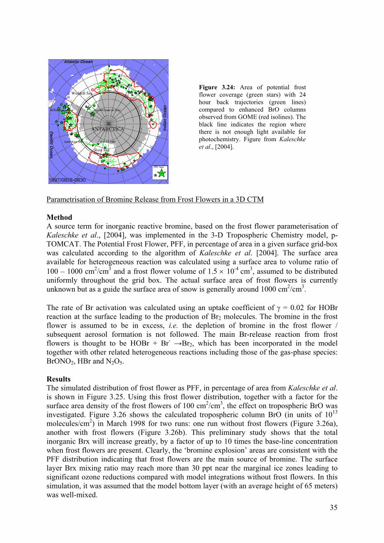
Figure 3.24: Area of potential frost flower coverage (green stars) with 24 hour back trajectories (green lines) compared to enhanced BrO columns observed from GOME (red isolines). The black line indicates the region where there is not enough light available for photochemistry. Figure from Kaleschke et al., [2004].

Parametrisation of Bromine Release from Frost Flowers in a 3D CTM

Method A source term for inorganic reactive bromine, based on the frost flower parameterisation of Kaleschke et al., [2004], was implemented in the 3-D Tropospheric Chemistry model, p-TOMCAT. The Potential Frost Flower, PFF, in percentage of area in a given surface grid-box was calculated according to the algorithm of Kaleschke et al. [2004]. The surface area available for heterogeneous reaction was calculated using a surface area to volume ratio of 100 – 1000 cm2/cm3 and a frost flower volume of 1.5 × 10-4 cm3, assumed to be distributed uniformly throughout the grid box. The actual surface area of frost flowers is currently unknown but as a guide the surface area of snow is generally around 1000 cm2/cm3.

The rate of Br activation was calculated using an uptake coefficient of γ = 0.02 for HOBr reaction at the surface leading to the production of Br2 molecules. The bromine in the frost flower is assumed to be in excess, i.e. the depletion of bromine in the frost flower / subsequent aerosol formation is not followed. The main Br-release reaction from frost flowers is thought to be HOBr + Br- →Br2, which has been incorporated in the model together with other related heterogeneous reactions including those of the gas-phase species: BrONO2, HBr and N2O5.

Results The simulated distribution of frost flower as PFF, in percentage of area from Kaleschke et al. is shown in Figure 3.25. Using this frost flower distribution, together with a factor for the surface area density of the frost flowers of 100 cm2/cm3, the effect on tropospheric BrO was investigated. Figure 3.26 shows the calculated tropospheric column BrO (in units of 1013 molecules/cm2) in March 1998 for two runs: one run without frost flowers (Figure 3.26a), another with frost flowers (Figure 3.26b). This preliminary study shows that the total inorganic Brx will increase greatly, by a factor of up to 10 times the base-line concentration when frost flowers are present. Clearly, the ‘bromine explosion’ areas are consistent with the PFF distribution indicating that frost flowers are the main source of bromine. The surface layer Brx mixing ratio may reach more than 30 ppt near the marginal ice zones leading to significant ozone reductions compared with model integrations without frost flowers. In this simulation, it was assumed that the model bottom layer (with an average height of 65 meters) was well-mixed.

35

These model results indicate that frost flowers are the main source of bromine during the ‘bromine explosion’ events. In addition, with frost flowers, the model may overcome the evident discrepancies between the modelled and observed ozone concentration in polar spring (namely, without frost flower Br-emission, the model overestimates ozone concentrations during polar spring compared with the observations).

Figure 3.25: Frost flower distribution as calculated after Kaleschke et al [2004].

3.2

BaVonotprevolfrothe

Wiof Satser

Figure 3.26a: The calculated tropospheric column BrO without frost flowers (1013

molecules/cm2) in March 1998

.2.5 Volcanoes as a Source of BrO

ckground lcanic eruptions are known to be a major sourcably HCl and HF. Recent studies by Bobrosence of large amounts of BrO with tight correcanic plume by ground-based spectroscopic mm the volcanic measurements are large, and p global tropospheric BrO background could be

thin the THALOZ project, upper limits of BrOvolcanic eruptions observed in measuremenellite measurements have the advantage of pies, but mainly due to their large footprint, th

Figure 3.26b: As Figure 3.26a but including the frost flower distribution given in Figure 3.25.

e of SO2 and some reactive halogen species wski et al. [2003] have also observed the lation to SO2 (factor Br:SO2 = 1:1000) in a easurements. The global emissions inferred otentially, the contribution of volcanoes to significant.

columns have been estimated for a number ts made by GOME and SCIAMACHY. roviding global coverage and a long time e sensitivity to SO2 and BrO in the lower

36

troposphere is limited. However, eruptive emissions of SO2 are easily observable in the satellite data, and BrO concentrations of the magnitude reported by the ground-based measurements are also well above the detection limit. Therefore, all available GOME and SCIAMACHY data have been searched for large SO2 signals, and all major events (SO2 above a threshold of 3.0E17 molecules cm-2) been analyzed for both SO2 and BrO. The results obtained for the eruptions covered by satellite overpasses over the Etna, Nyamuragira, Popocatepetl, and Reventador volcanoes show no correlation between enhanced volcanic SO2 during large eruptions and the corresponding BrO columns. Evidence for BrO enhancement was also not found in the vicinity of the Soufrière Hills volcanoes (see Figure 3.27). There was no major difference between GOME and SCIAMACHY measurements, although the latter have smaller ground scenes by a factor of 7-14. As an example, the correlation between BrO and SO2 is shown for the Nyamuragira volcano in Figure 3.28.

Thus, the satellite data are in apparent contradiction to ground-based observations. There are several possible explanations for the lack of signal in the satellite data:

1. A short lifetime of BrO in the volcanic plume, either through loss by reaction with, for example HO2, or through heterogeneous reactions on and in the volcanic aerosol present in the plumes. The ground-based measurements are taken close to the source, whereas the satellite averages over a large area (and thereby time). However, recent measurements have shown significant BrO concentrations at 25 km from the volcano, indicating that the lifetime cannot be very short.

2. Another possibility is a fundamental difference in BrO to SO2 ratio for the large eruptions studied here when compared to degassing as observed by Bobrowski et al. [2003]. In fact, there are indications from some measurements that Cl : SO2 ratios are different for eruptive events, and a similar effect could exist for Br.

3. It cannot be excluded that the observations by Bobrowski et al. [2003] were specific to the volcano and or the event studied. Extrapolation from this event to determine a global emission of bromine therefore requires caution.

This study focused on individual large eruptions and did not attempt to quantify the effect of degassing. Clearly, more ground-based measurements combined with satellite observations and studies of BrO chemistry are needed to resolve the differences between the ground-based and satellite observations of SO2 and BrO.

37

Figure 3.27: SCIAMACHY overpasses over the Soufrière Hills Volcano on the 13th and 14th July 2003 and corresponding slant column densities of SO2 and BrO (factored out by 1000) compared for these eruptions. The volcanic plume recorded on the 13th coincided with the volcano location and a BrO:SO2 of 8.29×10-5 was calculated. The ageing volcanic plume on the 14th July recorded a BrO:SO2 of 1.68×10-4 and the plume could be tracked several hundreds of kilometres from the volcanic site in a North-easterly direction.

Figure 3.28: Normalized slant column densities of volcanic SO2 and corresponding BrO from GOME (January 1996–June 2003) and SCIAMACHY data (August 2002–January 2004) for the Nyamuragira volcano. The dashed line is the correlation found by Bobrowski et al. [2003]. Figure from Afe et al., [2004]

38

3.3 Photochemistry

3.3.1 Method

A suite of experimental techniques has been used to investigate the photochemistry of iodine containing molecules.

Flash photolysis has been used to study I2/O3 mixtures. Multichannel and single channel time-resolved molecular absorption spectroscopy were used to detect the species of interest. Simultaneous measurement of all relevant species (low resolution: 1.3nm FWHM) was achieved.

A pulsed laser photolysis/cavity ring-down system has been used to investigate the photochemistry of iodine containing molecules. The ring-down (CRD) cavity was incorporated into a slow flow reactor.

The pulsed laser photolysis (PLP) technique has been coupled to transient absorption spectroscopy (TAS), resonance fluorescence (RF) and laser induced fluorescence (LIF) to measure photochemical and kinetic parameters for a number of iodine species.

3.3.2 Absorption Cross Sections

3.3.2.1 Absorption Cross Sections of IO

The absorption cross section of IO was determined within its 4,0 absorption feature at a wavelength of 427.2 nm using the method of pulsed photolytic generation combined with transient absorption spectroscopy. The relative shape of the 4,0 band was determined by measuring absorption profiles at ≈ 30 discrete wavelengths and a spectral resolution of 0.1

nm and is shown in Figure 3.29. When measured at sufficiently high resolution, this asymmetric band possesses a maximum cross section at 427.08 nm when experiments are carried out using air filled monochromators. The apparent discrepancy between this wavelength and the frequently quoted value of 427.2 nm is resolved when the wavelength shift from vacuum wavelengths (used by Harwood et al., [1997]) is taken into account. Note that at lower resolution the maximum shifts to longer wavelengths.

IO was generated by the reactions of O(3P) with either CF3I or I2 and the measured optical density traces converted to cross sections by measuring the initial concentration of O(3P) formed in the pulsed photolysis of NO2 (351 or 355 nm) or O2 (193 nm). This was achieved by

conversion of O(3P) to O3 and measurement of product O3 at 254 nm. Corrections for the branching ratio to IO formation in the reaction of O(3P) with CF3I, and other loss processes of

Figure 3.29: Shape of the 4,0 band of IO measured at 0.1 nm resolution. The wavelengths are in air.

39

O(3P) such as reaction with NO2 were taken into account by numerical simulation. The cross sections derived from the various experimental schemes are listed in Table 3.9.

The final value, derived from an average of the results using NO2 photolysis, is σ427.2nm (IO) = (3.55 ± 0.4) × 10-17 cm2 molecule-1. As shown in Table 3.9, the cross section at the peak of the absorption band is about 8 % higher, i.e. 3.8 × 10-17 cm2 molecule-1. This result is in good agreement with recent laser based studies of this cross section, once careful correction for effects of resolution and chemical calibration are coprepared, and will be submitted to a specia

Absorption cross section spectra for IO inand IO(v’←v”), v”>0 have also been deabsorption spectra of three other iodine oxthe spectra to absolute absorption cross sec

It has been proven that below 0.4 nm FWHcross sections of IO and OIO is less than 2other absorbers are present in the mixtureunaccounted species would be includedrigorously speaking they have to be cdetermination based on a mass balance appshow systematic structures and are gauss dscale of the fit all relevant absorbers are tak

The relative behaviour of the time curvesthermal equilibrium of the IO molecule is[IO] should therefore be equal to the Bolimplies that the experimentally determined

The values of σ(427.2 nm) determined hIUPAC recommendation of σ(427.2 nm) =

Scheme Pressure (Torr)

[O(3P)]

IOnm2.427σ b

NO2 / I2 (351 nm) 100 2.33 3.7 ± 0.3 300 4.86 3.65 ± 0.25 150 2.39 3.6 ± 0.4 150 1.83 3.4 ± 0.25 NO2 / CF3I (351 nm) 150 2.53 3.8 ± 0.55 150 1.86 3.5 ± 0.5 150 1.86 3.6 ± 0.55 NO2 / CF3I (355 nm) 150 1.16 3.8 ± 0.6 150 1.38 3.35 ± 0.45 150 1.71 3.3 ± 0.5 O2 / CF3I (193 nm) 105 4.85 3.3 ± 0.4 90 4.43 4.0 ± 0.4 100 6.22 3.2 ± 0.3 aUnits of 1012 molecules cm-3. bErrors include estimated systematic uncertainty.

Table 3.9: Summary of IO cross sections at 427.2 nm

nducted. A publication of these results has been l edition of the Journal of Photochemistry.

differently vibrationally excited states IO(v’←0), termined (see Figure 3.30). Broad structureless ides have been also obtained. Absolute scaling of tions could be determined for all but one.

M the influence of resolution over the absorption % and 5%, respectively. If the assumption that no were wrong, this would mean that the effect of in these absorption cross sections. Therefore, onsidered as lower in general with any other roach. Nevertheless, the residuals of the fits do not istributed, which confirms that at least in the time en into account.

observed for IO(4←0) and IO(3←1) shows that reached after about 10ms. The ratio of [IO*] to

tzmann factor, but it is found to be larger, which cross section of IO* is too small.

ere are in excellent agreement with the current (3.6±0.3)×10-17cm2 molecule-1.

40

300 320 340 360 380 400 420 440 460 480 500-0,10,00,10,20,3

300 320 340 360 380 400 420 440 460 480 500

0,0

0,5

1,0

1,5

2,0

2,5

300 320 340 360 380 400 420 440 460 480 5001E-30,010,1

110

IO(2←0)

optic

al d

ensi

ty

vacuum wavelength (nm)

2←0

abso

rptio

n cr

oss

sect

ion

(10-1

7 cm

2 /mol

ec)

IO(ν'←0)4←0σIO(4←0):

(2.13±0.2)10-17 cm2/molec at 1.3 nm FWHM(3.5 ±0.3)10-17 cm2/molec at 0.12 nm FWHM(427.19nm at 0.12nm FWHM)

rel.

erro

r

Figure 3.30: The extracted spectrum of ground state IO is plotted (top diagram) including the apparently reduced IO(2←0) band before and after correction. The UV end of the spectrum is clearly determined and structures are also seen in the continuum range. From the (4←0) to the red all troughs between bands return clearly to zero. The relative error of the spectrum is shown in the bottom diagram ranging around 1% for the largest part of the continuum and the band peaks. In the middle diagram the extraction for the irregularly behaving bands IO(2←0), IO(3←0) is plotted.

3.3.2.2 Absorption Cross Sections of OIO

A low resolution, full range reference spectrum has been obtained by partner 2 and is shown in Figure 3.31. The spectrum is free from other species to ±3%. Therefore, it will serve as a sound base for the future determination of higher resolved “pure spectra” of similarly low contributions from other remaining absorptions. The maximum of the spectrum is observed at 549.1 nm, with a cross section of (1.3 ± 0.3) × 10-17 cm2.

Figure 3.31 shows a higher resolution spectrum, calculated by dividing the fraction of OIO photobleached by the measured fluence of the photobleaching laser. OIO was generated from the IO self-reaction. The resulting cross section at 567.8 nm of (1.5 ± 0.2) × 10-17 cm2 is in excellent agreement with the absolute absorption cross section mentioned above.

The absorption spectrum of OIO in the strong visible absorption band between ~ 480 nm and 660 nm is well established, but there is considerable disagreement between the absolute cross sections determined in the different studies, even when experimental errors and the effects of instrument resolution are accounted for. The values of the absolute absorption cross section determined within THalOz will help resolve this disagreement.

41

450 500 550 600 650

-2,5

0,00E+

2,50E

5,00E

7,50E

1,00E

1,25E

1,50E

0E-018

000

-018

-018

-018

-017

-017

-017

450 500 550 600 6501E-30,010,1

110

100

vacuum wavelength (nm)

OIO

abso

rptio

n cr

oss

sect

ion

(cm

2 /mol

ec)

↓ (549.1±0.1)nm: (1.3±0.3)10-17 cm2/molec (0.35nm FWHM)

rel.

erro

r

Figure 3.31: The spectrum of OIO was extracted over different wavelength windows and then joined to form a contiguous spectrum. Both ends of the spectrum show clearly the end of the absorption and a smooth return to zero.

3.3.2.3 Absorption Cross Section of I2

Figure 3.32: The OIO photobleaching cross-section (___) with 1 σ error limits (……).

Recently, I2 was observed in the marine boundary layer by Differential Optical Absorption Spectroscopy [Saiz-Lopez and Plane, 2004]. A reference spectrum of the absolute absorption cross section of I2, at sufficiently high spectral resolution, was therefore required for DOAS retrieval. This spectrum was measured from 185 – 750 nm using a Fourier transform UV/Visible spectrometer [Saiz-Lopez et al., 2004], as shown in Figure 3.33. Figure 3.34 shows excellent agreement with a previous

measurement in the continuum region from 420 – 500 nm. The photolysis rate computed from this spectrum was shown to agree well with a laboratory measurement using a solar simulator [Saiz-Lopez et al., 2004].

42

5E-1825

Partner 2 has also determined the absorption cross section of iodine at 500nm to be (2.186±0.021)×10-18 cm2, in agreement with the value derived from the spectrum measured by Partner 3.

3.3.2.4 Absorption Cross Section of INO3

0

1E-18

2E-18

3E-18

4E-18

400 450 500 550 600Wavelength / nm

Cro

ss-s

ectio

n / c

m2 m

olec

ule-1

650

Tellinghuisen, 1973

this work

0

5

10

15

20

150 250 350 450 550 650 750Wavelength / nm

1018

Cro

ss-s

ectio

n / c

m2 m

olec

ule-1

Figure 3.34: Comparison of the I2 spectrum from this study at 0.1 nm resolution with the values calculated from the data reported by Tellinghuisen [1973].

Figure 3.33: Measured I2 absorption cross-section at 1 nm resolution.

In contrast to ClNO3 and BrNO3, INO3 has yet to be isolated and stored. In fact, it probably decomposes quite rapidly at temperatures above 290 K [Allan and Plane, 2002]. Consequently, INO3 was prepared in situ by the laser photolysis at 193 nm of NO2/CF3I mixtures, via the reaction sequence: NO2 + hν → NO + O; O + CF3I → IO + CF3; IO + NO2 (+N2) → INO3.

The absorption spectrum of INO3 was recorded using time-resolved Fourier transform spectroscopy in an absorption cell of length 125 cm. The absorption spectrum was recorded for about 20 ms after each laser pulse, as the gas flowed down the cell. The gas was exposed to between 1 and 3 laser shots, depending on flow velocity. The NO2 (and CF3I) removed when the laser pulse initiated the formation of INO3 were determined by fitting reference spectra to the raw optical density spectrum, as shown in Figure 3.35. The resulting residual spectrum is attributed to INO3 absorption, with an onset at 350 nm that is in excellent agreement with theory. The absolute cross section is obtained by using a full kinetic model of the chemistry in the reactor. This predicts that between 16 and 22% of the NO2 removed is converted to INO3, depending on the conditions. The average of three INO3 spectra, obtained under very different conditions, is plotted in Figure 3.36, along with an INO3 spectrum measured using a similar technique at the U. of Cambridge [Mössinger et al., 2002]. The latter is about a factor of 4 larger. The absorption cross section spectrum of BrNO3 is also shown, together with a spectrum red shifted by 0.78 eV, which is predicted by quantum theory to be the difference between the vertical transitions from the ground to the first excited states of BrNO3 and INO3. Although this shifted spectrum is in good accord with the INO3 spectrum from the present study, the UEA spectrum should be regarded as a lower limit, because wall losses of INO3 in the cell may have been significant. The photodissociation rate of INO3 for summer at midday, 50o latitude, is computed to be 1.8 × 10-3 s-1 using the UEA spectrum.

43

INO3 absorption cross section at 293 K

Wavelength / nm

200 250 300 350 400

Cro

ss se

ctio

n / c

m2 m

olec

ule-1

10-19

10-18

10-17 INO3 (U. Cambridge)

INO3 (UEA)

BrNO3 shifted by 0.78 eV

BrNO3

INO3 (NO3 photo-fragmentcross section - UEA)

Wavelength / nm

250 300 350 400 450

Opt

ical

den

sity

-0.06

-0.04

-0.02

0.00

0.02

0.04

0.06

Raw optical density spectrum Fitted NO2 and CF3I spectraResidual (spectrum of INO3)

Figure 3.36: Absorption cross section for INO3measured at UEA and UCam. For comparison, the BrNO3 spectrum is shown, together with a red shift of 0.78 eV predicted from quantum calculations to be the difference between the INO3 and BrNO3 spectra.

Figure 3.35: Deconvolution of the INO3spectrum by subtracting fitted reference optical densities of NO2 and CF3I from the raw optical density spectrum

3.3.2.5 Absorption Cross Section of Higher Oxides of Iodine

Up to three different broad band absorbers have been observed in the UV. They have been attributed to gas phase species, because no time dependent spectral shifts have been observed. Two of these oxides have been tentatively assigned to I2O2 and I2O3 following kinetic considerations. The third one could not be assigned. The possibility of it being IOO has been ruled out, as no evidence for its formation could be found from the photolysis experiments of I2/O2 mixtures. Spectroscopic vibrational analysis has shown that it does not originate from excited vibrational state IO(X2Π,v’’>1) (see above). A potential explanation for this species would be IO3, due to its early formation. Further experiments are required in order to unequivocally identify these higher iodine oxides.

44

3.3.3 Photochemistry and Quantum Yields

3.3.3.1 Photochemistry of IO

The high quality IO spectrum (see Figure 3.30) obtained in this work allows interesting spectroscopic analysis. The continuum of ground state IO was reproduced by overlapping Lorentz shaped bands, whose band strength was constrained to the systematic behaviour of calculated Franck-Condon factors (based on the Morse potential). In addition, two Gaussian continua representing two bound-free transitions had to be included to reproduce the observed continuum. As a result, this analysis yields the inference of two repulsive potentials from the observed Gaussian continua by using the so-called reflection method. Considering the inclination of tangents and the energy level of possible dissociation products I(2P3/2)+O(3P) and I(2P1/2)+O(3P) enables a plausible association of both. Another result is the first experimental determination of relative Franck-Condon factors for transitions from IO(X 2Πi), ν"=0 to IO(A 2Πi), ν'=0 to 18. A step further in this analysis will be the determination of experimental absolute Franck-Condon factors and the electronic transition moment.

By using the reflection method it could be shown that the third UV absorption mentioned earlier is not a continuum originating from excited vibrational state IO but originates from a further yet unidentified molecule, potentially IO3.

3.2.3.2 Photochemistry of OIO

Two of the partners have investigated the photodisociation behaviour of OIO. Their aim was to establish the overall and channel specific quantum yields of photodissociation. Partner 4 used pulsed laser photolysis combined with transient absorption spectroscopy and resonance fluorescence detection schemes. Partner 3 used a pulsed laser photolysis apparatus with detection by time-resolved cavity ring-down spectroscopy

Formation of I atoms A series of experiments were performed to look for I atoms formed by the 532 nm (YAG-Laser) or 562.3, 567.9 or 573.8 nm (Dye Laser) photolysis of OIO. The source

of OIO in these experiments was the IO-self reaction, which generates OIO at a significant yield. IO was generated in the reaction of O(3P) with CF3I, whereby O(3P) was generated in the 193 nm photolysis of a large excess of O3 (>1016 molecule cm-3). A typical data set is shown in Figure 3.37 in which the lower two curves show the IO and OIO time traces, recorded at 427.2 and 549.1 nm, respectively. The photolysis laser was triggered to fire at 0.5 ms after the excimer laser, close in time to the peak of the OIO profile, and the I atom profile (upper curve) was measured simultaneously. In most experiments, no prompt I atom formation was observed. In order to derive an upper limit to the quantum yield of I atom formation from these experiments, actinometry was performed using I2 photolysis at 532 nm

Figure 3.37: Experiment to investigate the photolysis of OIO at 532 nm. Details are given in the text.

45

as a well characterised source of I atoms. The I atom signal from a calibration experiment is displayed as the second trace from top, Figure. 3.37. The data were analysed using the expression

Φ whereby Isig(OIO) is the I atom signal from OIO

photolysis and Isig(I2) is the I atom signal from the actinometry with I2 and OD is the optical density of OIO or I2 prior to the laser pulse. From this expression, quantum yields for I atom formation of <0.24 (532 nm) and <0.02 (562.3 – 573.8 nm) were obtained.

)I()I()OIO()OIO( 2

I532OIO

532

I2532

2

I532 Φ⋅⋅=

ODOD

IsigIsig

Depletion of OIO In a second set of experiments, conducted at a laser wavelength of 532 nm, the change in OIO absorbance (measured at 610.2 nm) was monitored during photolysis. In this case, IO (precursor to OIO) was formed either in the photolysis of N2O at 193 nm, or O3 at 193 or 248 nm in the presence of I2 or CF3I. OIO was observed to be depleted by the laser pulse, and the degree of depopulation of the ground state OIO was seen to depend on the laser fluence. The experimental results obtained in a number of bath gases and at different pressures are summarised in Figure 3.38. The data at low laser fluence are consistent with a

a

6,0E+1

Ionloda

Pupwuwrp

0,E+000,0E+00 1,0E+13 2,0E+13 3,0E+13 4,0E+13 5,

F(1-exp(-OD532))

2,E-03

4,E-03

6,E-03

8,E-03

1,E-02

1,E-02

0E+13

Del

ta_O

D (6

10.2

nm

)

N2

HeN2HeN2He, 25 TorrN2, 25 Torr

Figure 3.38: Change in OIO optical density (OD) as afunction of laser fluence at 532 nm.

photolysis cross section at 610.2 nm of 1× 10-17 cm2 molecule-1, in broad

greement with the results from partner 3.

t is noteworthy that the depletion of OIO was not permanent, but a recovery over a timescale f ≈ 0.5 ms was usually observed. This agrees with the hypothesis (from UEA) that OIO is ot significantly dissociated by the laser, but the ground state is depopulated for a sufficient ength of time for a photo-bleaching cross section to be obtained. Differences in the timescale f recovery (< 2 µs in the case of the UEA experiments, see below) may be a result of using ifferent photolysis wavelengths, which result in population of different vibrational levels nd thus different relaxation rates.

artner 4 has also investigated possible removal processes of OIO. OIO was photobleached sing a Nd:YAG pumped dye laser. This laser was triggered, when the OIO concentration eaked, and was scanned over the region 558 – 578 nm. The degree of OIO photobleaching as measured by monitoring the OIO ground-state concentration 300 ns after this laser pulse, sing cavity ring-down on a vibronic band peak (λ = 567.808 nm). This monitoring avelength was selected to minimise interference from I2, which absorbs over the same

egion, and is generated by recombination of I atoms produced in the formation and hotolysis of OIO, as well as subsequent iodine oxide chemistry.

46

The same experiment was then performed in the time d

In broad terms, the two studies show

omain by varying the delay between the photobleaching and the ring-down lasers, in order to determine the fraction of photobleached OIO that reappeared at longer times (> 1µs). As shown in Figure 3.39, most of the initially bleached OIO reappears, and we conclude that the photolysis yield at 562 nm is less than 10%.

that OIO is remarkably stable with respect to dissociation. At present, the results do not rule out that a small quantum yield for dissociation (i.e. less that 0.05) could provide the major fate of OIO in the atmosphere.

3.3.3.3 Photochemistry of INO3 els of INO3 that are in prin

Energy

Time / µs

1 10Frac

tion

of O

IO re

mov

ed a

fter

to-a

bsor

ptio

nph

o

0.2

-0.1

0.0

0.1

0.340 torrr N2Initial removal = 0.26

Average remainingOIO = 5 x 10-3

Figure 3.39: Fraction of OIO removed following absorption at 562 nm, as a function of time after the laser pulse. The reappearance of OIO can be modelled assuming V-T transfer from OIO to N2, with an average energy of about 120 cm-1 per collision.

There are three photolytic chann ciple accessible at wavelengths

threshold (from quantum theory)

he photofragments of INO3 at 248 nm have been studied. As before, INO3 was produced by

The cavity ringdown system was then used to detect the NO3 photofragment and indicates

A set of quantum theory calculations on the iodine oxides has been performed. These

below 350 nm, although the third has a large barrier to internal rearrangement:

INO3 + hν → IO + NO2 105 ± 10 kJ mol-1 → I + NO3 137 ± 19 kJ mol-1 → OIO + NO 166 ± 20 kJ mol-1

Tthe 193 nm photolysis of NO2 in the presence of CF3I. After 800 µs, the INO3 was photolysed by a 248 nm excimer laser. The yield of IO was measured by LIF at 445 nm, using a dye laser that crossed the reaction volume and a photomultiplier tube that was mounted perpendicular to the reactor axis. Modelling of the observed LIF spectra indicates an upper limit to the IO + NO2 photolysis channel of 0.5%.

that the NO3 yield is about 30%. However, a sizable fraction of the hot NO3 produced by 248 nm photolysis of INO3 is likely to dissociate to NO2 + O, rather than be quenched and observed. Analogous behaviour is seen in the photochemistry of BrNO3 and ClNO3 at 248 nm [Harwood et al., 1998; Zou et al., 2002]. Thus, we conclude that I + NO3 is the only major photolysis channel of INO3 (at 248 nm). Further details of this study are given in Appendix 2.1.

calculations are reported in appendix 2.2 and include calculated dipole moments, vertical electronic transitions (wavelength and oscillator strength f), rotational constants, vibrational frequencies and heats of formations for a series of iodine oxides. Predicted infrared spectra for the iodine oxides are also given.

47

3.3.4 Kinetics

The rate coefficients for many reactions involving iodine containing species have been determined and branching measured for a number of reactions.

3.3.4.1 Self-reaction of IO: Kinetics and Products

A large number of experiments were conducted to determine the overall rate constant for the IO self reaction, and also to obtain the branching ratio into possible product channels at 298 K. The possible reaction pathways are:

IO + IO → OIO + I → 2 I + O2 → I2 + O2

IO + IO + M → I2O2 + M

Overall rate constant (low O3 experiments) The overall rate coefficient is obtained in experiments in N2 or air bath gas in which a low concentration of O3 (10-12 molecule cm-3) was totally dissociated in the laser pulse, and the resultant O(3P) allowed to react with I2. Rate coefficients were obtained at pressures between 20 and 600 Torr, and displayed no dependence on this parameter. The pressure independent, overall rate coefficient is (0.97 ± 0.07) × 10-10 cm3 molecule-1 s-1.

Branching ratio determination By conducting the experiments in a large concentration of ozone, the I atom formation channels are suppressed as IO is rapidly reformed, resulting in a reduction in the apparent rate constant. For these experiments the IO source was either the photolysis of I2 or CH2I2. The decays of IO were 2nd-order over the range of pressures 20 < p / Torr < 760, enabling the parameter k*, the rate of reaction to non I-atom products to be determined. The product yield (per IO reacting) of non-I atoms is given by the ratio k*/k where k is the rate coefficient for the overall self-reaction of IO (see above). The results are summarised in Figure 3.40.

Figure 3.41: Simultaneous measurement of IO and I atoms at 20 Torr.

0,0

0,2

0,4

0,6

0,8

1,0

0 200 400 600 800

p / Torr

α (y

ield

per

IO re

actin

g)

non I-atom, CH2I2 / 351 nm

non I-atom, I2 / 532 nm

I-atoms, I2 / 532 nm

OIO, O3 / 248 nm

Figure 3.40: Products yields from the IO self-reaction as a function of total pressure.

48

In a further set of experiments (Figure 3.41), a calibrated resonance fluorescence detection system for I-atoms was coupled to the existing PLP-transient absorption apparatus to enable simultaneous monitoring of I, IO and OIO. Incorporation of the improved rate data for elementary reactions of O and I-atoms (see below) into a photochemical model allowed the direct determination of the product yield (per IO reacting) of I-atoms (αI) at 20 Torr.

At higher pressures the model was unable to simulate the I and IO profiles, probably due to IOx catalysed I-atom recombination competing with I + O3. Further, the determination of an absorption cross-section for OIO enabled observed optical densities of OIO to be placed on an absolute concentration scale. Estimates for the product yield of OIO per IO reacting (αOIO) were determined from data in which IO and OIO were monitored simultaneously following 248 nm photolysis of O3 / I2 mixtures (Figure 3.40).

Observation of a pressure dependence for these product yields, determined in 4 different photochemical systems, provides strong evidence for the IO self-reaction mechanism proceeding via an association complex (most likely IOIO) followed by elimination of I to form OIO or stabilisation of the dimer at higher pressures. Important results derived from the data in Figure 3.40 include αΟΙΟ = (0.2 ± 0.1), αΙ = (0.15±0.1) at 760 Torr. These results are summarised in the Table 3.10 below:

Self-reaction of IO: kinetics and products (second study) Partner 3 has also studied the IO self reaction as part of their kinetic analysis of the chemical system established following flash photolysis of I2/O3 mixtures. Approximately 60 experiments were performed over a range of ozone (1-30×1014 molecule cm-3) and iodine (0.06-5×1014 molecule cm-3) concentrations. Oxygen and nitrogen were used as buffer gases, giving total reactor pressures of between 40 and 400 mbar.

In all experiments the O3 concentration is in excess over any other species, and in particular over [I]. Therefore pseudo-first order decays of I were expected. Nevertheless, the logarithmic plot of [I] against time shows two sections, the first one being linear and corresponding to I+O3→IO+O2. A rate coefficient for this reaction has been determined from this first section and is given in the next section. The second section observed is due to the coupling of I+O3→IO+O2 and most likely the I-atom producing channels of IO+IO.

Simple kinetic analysis does not allow any further determination of rate constants. In general IO does not present second order kinetics in the presence of O3 due to I atom recycling. If I and IO do not undergo further reactions, their rate equations would be respectively:

To have second order kinetics in IO it would be necessary to reach steady state of I:

1][ k

dtIOd

=

31 ][[][ IOkdt

Id−=

22 ][2]][ IOkI −

222 ])[5.0( IOkk ba +

22 ][2])[5.0(2] IOkIOkkk =−+= 22222

2231[])[5.0(2]][[0][dtIOdIOkkIOk

dtId

noIbaba ⇒+=⇒=

2]+

3[O

49

Only in the particular case of high [O3] does the recycling of I seem to be fast enough to fulfil this condition ([I] is always nearly 0). If other reactions like IO+OIO are taking place the decay of IO cannot in general be second order.

The logarithmic plot of [OIO] against time shows two sections, the second one being fairly linear. The reaction O3 + OIO could help explain the observed time dependence of OIO, but the rate coefficient required is large enough to be inconsistent with observation of OIO in the MBL. For this reason the reaction OIO+O3 is not considered.

The failure of the simple kinetic analysis made it necessary to use a chemical model and simultaneously fit modelled concentration curves to the observed [I2], [I], [IO] and [OIO]. Well established rate constants were kept fixed. The reaction scheme considered included the four branches of the IO self reaction, I + O3, OIO + IO and OIO + OIO.

The branching ratios obtained for the IO self reaction are shown in Figure 3.42. The broken lines show that the extrapolation of our results towards low pressures and atmospheric pressure are in good agreement with the only two previously published results. A comparison with the data determined by Partner 4 is given in Table 3.10 below. The results from Partner 3 are still preliminary. Analysis of additional datasets is ongoing.

Figure 3.42: Pressure dependence of the branching ratios of the IO self reaction. Black data points this work; Red data points Vipond et al.; Blue data points Bloss et al.;Circles k(I+OIO)/ktot; Squares k(2I+O2)/ktot; Stars k(I2O2)/ktot; Diamonds k(I2+O2)/ktot; Broken lines are extrapolations of the current work to high and low pressures. During their study of the spectrum of OIO Partner 3 modelled the observed variation of the OIO concentration with time and derived a branching ratio for OIO production in the IO self reaction of 0.32±0.14 at 40 Torr N2.

50

Branching ratio Reaction

Products Partner 41 Partner 32

IO + IO → I + OIO 0.4 ± 0.1 0.45 ± 0.04 → 2 I + O2 < 0.15 0.26 ± 0.04 → I2 + O2 n/a 0.23 ± 0.06 IO + IO + M → I2O2 + M 0.57 ± 0.16 0.06 ± 0.05

Notes: 1Overall rate coefficient is (0.97 ± 0.07)×10-10 cm3 molecule-1 s-1 2Errors applicable to all data in Figure 18 Table 3.10: Kinetics and products of the IO self reaction at 298 K with 400 mbar N2

3.3.4.2 Reactions Involving I Atoms

Three reactions consuming and generating I atoms were studied using the laser photolysis – resonance fluorescence technique:

I + O3 → IO + O2 O(3P) + I2 → IO + I I + NO2 + M → INO2 + M The study of these reactions served to characterise the resonance fluorescence set up for I atoms, and also helped strengthen the surprisingly weak database on these important reactions.

All rate coefficients were derived by monitoring either exponential I atom decays (I + O3 and I + NO2) or I atom formation in O(3P) + I2. The accuracy of the rate coefficients was enhanced by online optical absorption spectroscopy to derive the concentration of the excess reagent, O3 (254 nm), I2 (500 nm) or NO2. (400 nm). The rate coefficient for this reaction at 298 K was found to be: k(I+O3) = (1.28 ± 0.06)×10-12 cm3 molecule-1 s-1. Partner 2 determined a value of k(I+O3) = (1.17±0.06)×10-12 cm3molecule-1s-1 from the simultaneous fit of the O3/I2 chemical system following flash photolysis. Partner 4 also obtained a similar quality data set for O(3P) + I2, with a rate coefficient derived as (1.2 ±0.1) × 10-10 cm3 molecule-1 s-1. For the termolecular reaction of I with NO2, a strong pressure dependence was found in both He and N2 bath gases. The data set of Partner 4, at pressures between 19 and 610 Torr, was combined with those of van den Bergh and Troe, [1976] and used to calculate centre broadening factors of Fc(He) = 0.43 and Fc (N2) = 0.48 and high and low pressure limiting rate coefficients with k∞ = 1.1 × 10-10 cm3 molecule-1 s-1, k0(He) = 1.48 × 10-31 cm6 molecule-2 s-1 and k0(N2) = 3.2 × 10-31 cm6 molecule-2 s-1. The rate coefficients for O(3P) + I2 and I + O3 have been used to analyse IO and I atom profiles in the studies of the IO self reaction (see above). This work has been published in Tucceri et al., [2005] and incorporated in the latest IUPAC recommendations.

3.3.4.3 Reaction of IO with CH3SCH3 and CH2I with O2

A pulsed laser photolysis / pulsed laser induced fluorescence (PLP-LIF) experiment has recently been commissioned to enable sensitive (~ 1010 molecule cm-3) detection of IO. This set up has been used to investigate the kinetics of the bimolecular reactions IO + CH3SCH3 → (products) and CH2I + O2 → IO + HCHO, which may, if fast enough, be of atmospheric

51

interest. Two recent publications Nakano et al., [2003] and Enami et al., [2004] reported large rate coefficients for these reactions.

IO + CH3SCH3 The reaction of IO with CH3SCH3 was studied using PLP with LIF detection of IO following excitation at 445 nm. IO was generated in the reaction of O(3P) with CH3I, with O(3P) formed in the 351 nm photolysis of NO2. This scheme avoids photolysis of the large excess of CH3SCH3 or CH3I.

IO decays were observed to be strictly exponential and the pseudo first-order rate constant depended linearly on the concentration of CH3SCH3. In contrast to the work of Enami et al, the rate constant obtained was found to be independent of pressure, with a value at 298 K of (1.4 ± 0.3) × 10-14 cm3 molecule-1 s-1, in good agreement with the more recent flow tube studies of this reaction. The temperature dependence of the reaction was also investigated between 350 and 250 K, and revealed a barrier of ≈ 8 kJmol-1, again in contrast to Enami et al, who determined a negative temperature dependence.

Further, experiments carried out in the presence of sufficient O3 to scavenge any I atoms indicated that the major, if not sole, reaction channel forms CH3S(O)CH3 + I.

The results from this study, which are in good agreement with an independent measurement from the University of Leeds, indicate that the reaction with IO is not a significant loss process for CH3SCH3 in the marine boundary layer. The results of this study are presently being summarised for publication.

Reaction of CH2I with O2 The reaction of CH2I with O2 has been proposed to form IO directly, rather than a peroxy radical ICH2O2.

CH2I + O2 → IO + HCHO Should this be correct, then the photolysis of CH2I2 can be a source of two I atoms in the absence of NOx. Therefore, experiments were conducted in which CH2I2 was photolysed at 351 nm to generate CH2I in the presence of varying amounts of O2. Although IO was indeed formed in this chemical system, several observations (i.e. a quadratic dependence of the IO signal strength on laser energy and the lack of dependence of its decay rate on O2) indicated that it was formed in secondary reactions of ICH2O2 and not directly.

3.3.4.4 Reactions of O(3P) with RI

A number of reactions of O(3P) with alkyl iodides were investigated in order to assess their suitability as IO source reactions in studies of IO kinetics. The reactions studied are listed in Table 3.11, as are the overall rate coefficients, expressed in Arrhenius form. The experiments were carried out at temperatures between 223 and 363 K, using pulsed laser photolytic generation of O(3P) coupled to its detection resonance fluorescence or detection of IO by transient absorption spectroscopy. The reactions were carried out with a large excess concentration of the alkyl iodide, i.e. pseudo first-order conditions. Optical measurement of [RI] enhanced the accuracy of the rate coefficients obtained. With the exception of O(3P) + CF3I and O(3P) + CH2I2, all other rate coefficients display a negative temperature dependence, which highlights the importance of association complex formation in reactions 52

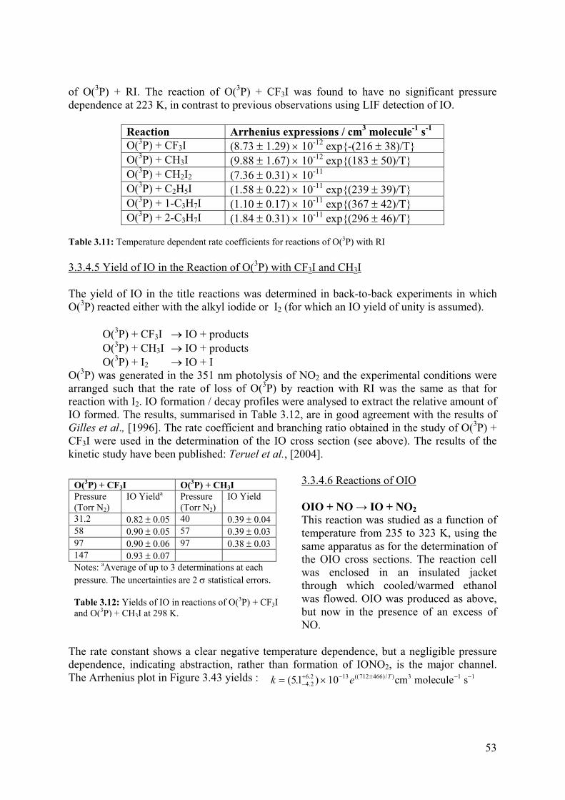
of O(3P) + RI. The reaction of O(3P) + CF3I was found to have no significant pressure dependence at 223 K, in contrast to previous observations using LIF detection of IO.

Reaction Arrhenius expressions / cm3 molecule-1 s-1 O(3P) + CF3I (8.73 ± 1.29) × 10-12 exp-(216 ± 38)/T O(3P) + CH3I (9.88 ± 1.67) × 10-12 exp(183 ± 50)/T O(3P) + CH2I2 (7.36 ± 0.31) × 10-11 O(3P) + C2H5I (1.58 ± 0.22) × 10-11 exp(239 ± 39)/T O(3P) + 1-C3H7I (1.10 ± 0.17) × 10-11 exp(367 ± 42)/T O(3P) + 2-C3H7I (1.84 ± 0.31) × 10-11 exp(296 ± 46)/T

Table 3.11: Temperature dependent rate coefficients for reactions of O(3P) with RI

3.3.4.5 Yield of IO in the Reaction of O(3P) with CF3I and CH3I

The yield of IO in the title reactions was determined in back-to-back experiments in which O(3P) reacted either with the alkyl iodide or I2 (for which an IO yield of unity is assumed).

O(3P) + CF3I → IO + products O(3P) + CH3I → IO + products O(3P) + I2 → IO + I O(3P) was generated in the 351 nm photolysis of NO2 and the experimental conditions were arranged such that the rate of loss of O(3P) by reaction with RI was the same as that for reaction with I2. IO formation / decay profiles were analysed to extract the relative amount of IO formed. The results, summarised in Table 3.12, are in good agreement with the results of Gilles et al., [1996]. The rate coefficient and branching ratio obtained in the study of O(3P) + CF3I were used in the determination of the IO cross section (see above). The results of the kinetic study have been published: Teruel et al., [2004].

3.3.4.6 Reactions of OIO

OIO + NO → IO + NO2 This reaction was studied as a function of temperature from 235 to 323 K, using the same apparatus as for the determination of the OIO cross sections. The reaction cell was enclosed in an insulated jacket through which cooled/warmed ethanol was flowed. OIO was produced as above, but now in the presence of an excess of

O(3P) + CF3I O(3P) + CH3I Pressure (Torr N2)

IO Yielda Pressure (Torr N2)

IO Yield

31.2 0.82 ± 0.05 40 0.39 ± 0.04 58 0.90 ± 0.05 57 0.39 ± 0.03 97 0.90 ± 0.06 97 0.38 ± 0.03 147 0.93 ± 0.07 Notes: aAverage of up to 3 determinations at each pressure. The uncertainties are 2 σ statistical errors. Table 3.12: Yields of IO in reactions of O(3P) + CF3I and O(3P) + CH3I at 298 K.

NO.

The rate constant shows a clear negative temperature dependence, but a negligible pressure dependence, indicating abstraction, rather than formation of IONO2, is the major channel. The Arrhenius plot in Figure 3.43 yields : k e T= ×−

+ − ± − −(5. ).. (( ) / )1 104 2

6 2 13 712 466 cm molecule s3 1 1

53

Figure 3.43: Arrhenius plot for the reaction between OIO and NO. The solid line is a linear regression though the data points, and the broken line is a fit from RRKM theory on an ab initio quantum potential energy surface.

Other reactions of OIO Reaction coefficients could be estimated from the simultaneous fit by partner 2 to their data yielding k(IO+OIO)=(1-2)×10-10 molecule-1s-1cm3 and k(OIO+OIO)=(1-3)×10-10 molecule-1s-

1cm3. A slight pressure dependence was observed, but it was smaller than the estimated error limits. Partner 3 could also extract information from the observed removal rate of OIO from their system. In this case the decay of OIO was attributed, by process of elimination and backed up by theoretical calculations, to be due to the reaction OIO + I (+ N2) → IOIO, with a rate constant of 1.5 × 10-10 cm3 s-1 at 40 Torr N2 and 293 K.

3.3.4.7 Formation of Higher Iodine Oxides, Deposits and Particles

In photolysis mixtures of I2/O3, it has been observed that the formation of higher oxides depends strongly on the initial mixing ratio [I2]/[O3]. If after the photolysis of [I2] the amount of I atoms is large compared to [O3], then it is observed that more [I2] is recovered and less deposit formed. The other way round, if [O3]>[I], then [I2] recovery is small or even negligible and strong deposit formation is observed. This is most likely to be due to the competition between I+O3→IO+O2 and I atom abstraction from the higher iodine oxides (IxOy+I→I2+Ix-1Oy).

A hygroscopic, white deposit has been collected after experiments with high ozone concentration. The FTIR analysis showed that this substance contained the stable oxide I2O5. Microscopic analysis of the deposit showed needle shaped crystals which have been reported for I2O5. Because of its hygroscopicity, this compound is a potential candidate for condensation nuclei formation. A possible pathway to I2O5 would be:

IO+OIO+M →I2O3+M I2O3+O3→ I2O4+O2

OIO+OIO+M →I2O4+M I2O4+O3→ I2O5+O2

Therefore, further work is necessary to spectrally identify the higher iodine oxides and to characterize its chemistry.

54

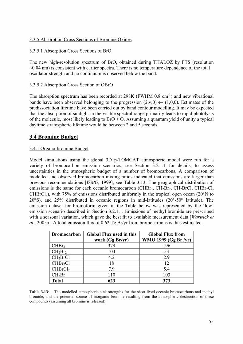
3.3.5 Absorption Cross Sections of Bromine Oxides

3.3.5.1 Absorption Cross Sections of BrO

The new high-resolution spectrum of BrO, obtained during THALOZ by FTS (resolution ~0.04 nm) is consistent with earlier spectra. There is no temperature dependence of the total oscillator strength and no continuum is observed below the band.

3.3.5.2 Absorption Cross Section of OBrO

The absorption spectrum has been recorded at 298K (FWHM 0.8 cm-1) and new vibrational bands have been observed belonging to the progression (2,ν,0) ← (1,0,0). Estimates of the predissociation lifetime have been carried out by band contour modelling. It may be expected that the absorption of sunlight in the visible spectral range primarily leads to rapid photolysis of the molecule, most likely leading to BrO + O. Assuming a quantum yield of unity a typical daytime stratospheric lifetime would be between 2 and 5 seconds.

3.4 Bromine Budget

3.4.1 Organo-bromine Budget

Model simulations using the global 3D p-TOMCAT atmospheric model were run for a variety of bromocarbon emission scenarios, see Section 3.2.1.1 for details, to assess uncertainties in the atmospheric budget of a number of bromocarbons. A comparison of modelled and observed bromocarbon mixing ratios indicated that emissions are larger than previous recommendations [WMO, 1999], see Table 3.13. The geographical distribution of emissions is the same for each oceanic bromocarbon (CHBr3, CH2Br2, CH2BrCl, CHBr2Cl, CHBrCl2), with 75% of emissions distributed uniformly in the tropical open ocean (20°N to 20°S), and 25% distributed in oceanic regions in mid-latitudes (20°-50° latitude). The emission dataset for bromoform given in the Table below was represented by the ‘low’ emission scenario described in Section 3.2.1.1. Emissions of methyl bromide are prescribed with a seasonal variation, which gave the best fit to available measurement data [Warwick et al., 2005a]. A total emission flux of 0.62 Tg Br/yr from bromocarbons is thus estimated.

Bromocarbon Global Flux used in this work (Gg Br/yr)

Global Flux from WMO 1999 (Gg Br /yr)

CHBr3 379 196 CH2Br2 104 53 CH2BrCl 4.2 2.9 CHBr2Cl 18 12 CHBrCl2 7.9 5.4 CH3Br 110 103 Total 623 373

Table 3.13: – The modelled atmospheric sink strengths for the short-lived oceanic bromocarbons and methyl bromide, and the potential source of inorganic bromine resulting from the atmospheric destruction of these compounds (assuming all bromine is released).

55

3.4.2 Inorganic Bromine Budget

Method The 3-D global model p-TOMCAT has been adapted to contain gas-phase bromine chemistry and bromine sources. The organic bromine sources have been modelled following the work of Warwick et al., Section 3.2.2.1. The parametrisation of the inorganic bromine source from sea salt is described in Section 3.2.2.3. The chemical scheme is identical to the bromine scheme contained in the box model, which is described in detail in the first THALOZ annual report. Further details of the model and the different scenarios applied may also be found in Yang et al. [2005].

Results The total inorganic gas-phase bromine Brx (=[HBr] +[HOBr] +[BrONO2] +[BrO] +[Br] +[BrNO2] +2[Br2]) calculated in the model, using the sea salt production of Smith et al. [1993], see Section 3.2.2.3, is shown in Figure 3.44 for March (a), June (b), September (c) and December (d). Highest Brx mixing ratios (4-8 ppt) appear in the lower troposphere of the mid- to high latitudes of each hemisphere with decreasing mixing ratios with altitude (down to about 2-3 ppt in the upper troposphere). The lowest Brx (1-2 ppt) is in the tropical upper troposphere. These lowest values are likely to be due to the weak surface wind at the equator, and, hence, small sea salt Br-emission, together with a high rate of precipitation scavenging. The relatively low mixing ratios of Brx during the NH summer (June and September) correspond to a relatively low sea salt production and more rainfall in the summer. Photochemistry also has an effect on the seasonal cycle. For example, HBr is formed more rapidly in summer, and therefore the deposition flux of Brx will be more rapid. In the SH, the lower wintertime Brx (~2 ppt) in June (Figure 3.44b) corresponds to the period when the bromine depletion factor, DF, is lowest (see Figure 3.22) and the enhanced Brx in December (Figure 3.44d) corresponds to the highest DF values.

Figure 3.45 shows the horizontal distribution of surface Brx concentrations for (a) March, (b) June, (c) September and (d) December. Generally, high Brx (>4ppt) is mostly formed in mid- to high latitudes with maximum values of 20 ppt in some regions. The exception is in the SH during June where Brx is less than 2 ppt, corresponding to the lowest DF values. Brx in equatorial areas and over continents is very low, consistent with low Br-emissions. In the SH, the highest Brx is in austral winter (Figure 3.45d) and spring (Figure 3.45a), with low Brx in the summer (Figure 3.45b) and autumn (Figure 3.45c). It is interesting to note that the North Atlantic has a higher Brx level than the North Pacific, which produces a large Brx gradient between the North Atlantic and Europe. These calculated reactive bromine amounts agree broadly with the available observations in the marine boundary layer collected by Sander et al. [2003].

56

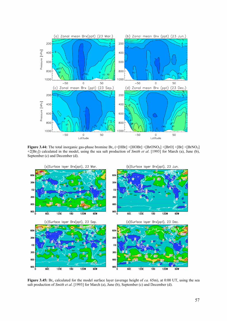
Figure 3.44: The total inorganic gas-phase bromine Brx (=[HBr] +[HOBr] +[BrONO2] +[BrO] +[Br] +[BrNO2] +2[Br2]) calculated in the model, using the sea salt production of Smith et al. [1993] for March (a), June (b), September (c) and December (d).

Figure 3.45: Brx calculated for the model surface layer (average height of ca. 65m), at 0:00 UT, using the sea salt production of Smith et al. [1993] for March (a), June (b), September (c) and December (d).

57

3.5 Ozone Loss

3.5.1 The effect of Background Concentrations of Reactive Bromine on Tropospheric Ozone.

Background In this study, the effect of background concentrations of tropospheric bromine, as determined in Section 3.4, on ozone was investigated. The specific ozone loss, due to reactions releasing reactive bromine, in the Polar Sea-ice zones, was not included in this study. A separate study showing the effect of autocatalytic bromine release on ozone is shown in Section 3.5.2. The method used is identical to that in Section 3.4.

Results In the presence of BrO and Br, ozone is lost through catalytic reactions simplified as Br + O3 → BrO + O2, BrO + HO2 →HOBr + O2 (rate determining) and HOBr + hν → Br +OH. The loss rate is related to the total concentration of inorganic bromine (Brx), and the fraction present as Br and BrO. From a comparison between runs with and without bromine chemistry, it is found that, in the Northern Hemisphere, the net ozone reduction is 4-6% in general and in the Southern Hemisphere a much high ozone reduction occurs with a maximum loss of about 30% in the polar regions, Figure 3.46. On average, the Southern Hemisphere has a larger net ozone reduction due to bromine chemistry than the Northern Hemisphere. The bromine-related ozone loss is also related to solar irradiance. For example, the maximum ozone reduction in the Northern Hemisphere (>10%) occurs in the polar region for June (Figure 3.46b) and corresponds not to the highest Brx levels but to the longest periods of sunlight (polar day at >68°N). Similarly, the largest ozone loss in the Southern Hemisphere polar region in December (Figure 3.46d) also corresponds to polar day. A small ozone loss of about 6% in the Southern Hemisphere is seen in June due to the low DF values used in the model. Clearly, the net ozone loss through bromine chemistry is related not only to Brx levels but also to the solar radiance.

Figure 3.46: The zonal mean ozone change due to bromine chemistry from a comparison of a model including bromine chemistry with one without bromine chemistry, on 23 March (a), June (b), September (c) and December (d).

58

3.5.2 Investigation of the Autocatalytic Release of Bromine in the Polar Sea-ice Zones

Background The destruction of boundary layer tropospheric ozone in Polar Spring was first noted in the late 1980’s. It was subsequently noted that inorganic bromine mixing ratios were found to be elevated at the same time as the bromine depletion. In Section 3.1, the increased BrO in Polar springtime, as measured by the satellite instruments may be seen (Figure 3.3). This study shows, using a simple model, some factors that effect the ozone depletion and the increase in BrO during ‘bromine explosion events’.

Method Initial studies to investigate the phenomenon of ‘bromine explosion’, together with ozone depletion in the Polar springtime boundary layer, has focussed on the use of a box model, as part of the M1 Work Package. The model itself is described in detail elsewhere, see for example the THALOZ first annual report. The bromine for the ‘bromine explosion’ was assumed to originate from saline aerosols, due to the reaction of HOBr + Br- →Br2, and it was assumed that the aerosol bromide was in excess, i.e. change in aerosol composition was not followed. The effects of (1) changing aerosol surface area, (2) changing solar intensity, (3) changing CH2O mixing ratio and (4) entrainment of ozone from aloft were considered.

Results Considering model runs at Polar Spring time (75N, Julian days 110 – 120) the formation of BrO and depletion of ozone has been found to be positively related to the surface area of aerosols and negatively related to solar radiation. A base case with 10µm2/cm3 and no cloud cover shows little change in the ozone mixing ratio with time. If the aerosol surface area is increased to 50µm2/cm3, then a rapid ozone loss is produced and the ozone mixing ratio drops from around 40 ppb to 10 ppb in 24 hours. A fall in ozone mixing ratio is also observed, at the lower aerosol surface area, if solar intensity is reduced from the clear sky scenario. With 90% cloud cover the fall in ozone mixing ratio is equal to that observed with the increased aerosol surface area but it takes around 4 days to occur.

It should be noted that these model runs produce minimum ozone mixing ratios around 10 ppb, over the period studied. Field measurements show that ozone, in some cases is below the detection limit of commonly used instruments i.e. less than 1 ppb. In the model, such low ozone mixing ratios are only simulated when formaldehyde mixing ratios are lowered. If HCHO emissions are stopped, the HCHO mixing ratio will fall to between 10-30 ppt and the ozone mixing ratio will fall to the low mixing ratios observed in field studies.

59

The effect of ozone entrainment, from above the boundary layer, on the formation of BrO is shown in Figure 3.47. The simulation is for a location of 75S during the austral spring. A mean surface area density, for sea-salt aerosols, of 50µm2/cm3 is used in the simulation,

together with clear sky conditions. The black ozone line

Fodben

3

InToopcbinstore

is for a model run without any bromine chemistry. It can be seen that once the ozone has been consumed, due to the ‘bromine explosion’ chemistry, no further BrO is produced and any remaining BrO is rapidly removed to more stable bromine compounds. In order to sustain BrO mixing ratios, entrainment of ozone from aloft is required. From Figure 3.47 it can be seen that, at least with these mixing ratios, the BrO mixing ratio is almost directly related to the ozone mixing ratio within the boundary layer. Therefore, the surface BrO concentration in the boundary layer is related to the stability of Boundary Layer: with a less stable boundary layer there is a potential to maintain higher BrO mixing ratios.

igure 3.47: Box model calculations to show the effect of ozone entrainment, from above the boundary layer, n the formation of BrO. The simulation is for a location of 75S during the austral spring. A mean surface area ensity, for sea-salt aerosols, of 50µm2/cm3 is used in the simulation, together with clear sky conditions. The lack ozone line is for a model run without any bromine chemistry. The brown line is without any ozone trainment; the pink line with a large ozone entrainment rate and the blue line for a smaller entrainment rate.

.6 Impacts on Radiative Forcing of Climate

troduction he climate impact of reactive halogens has been studied, within THALOZ using the results f global CTM calculations of the effect of bromine chemistry on ozone, combined with an ff-line climate model. However, due to their potential importance in climate, the results of hotochemical studies described in Section 3.3 should also be briefly noted here. During the ourse of the project a study by Enami et al., [2004] raised the possibility that the reaction etween IO and DMS could be important. Since oxidation of DMS has a recognised fluence on climate due to the formation of particles and, hence, cloud properties. However, udy, by Partner 4, found that the reaction was too slow to be of atmospheric relevance. The ther reactions that have been found to be of potential importance in climate change are those lating to the formation of particles of iodine oxide. The exact mechanism for the reaction is

60

not yet well-understood but it is clear that, with the right conditions, iodine oxide particles may be formed in the marine atmosphere and, thus, could influence cloud properties.

3.6.1 Radiative Forcing Calculations

Introduction Radiative forcing is a measure of the perturbation of the planetary radiation budget following a change in atmospheric composition, in this case, in ozone concentration. It provides a useful first-order estimate of the importance of a climate change mechanism and has been used as such for about 15 years. More recently, it has begun to be used in a 'legislative framework' as it underpins the use of Global Warming Potential (GWP); the GWP is used within the Kyoto Protocol to allow countries to compare emissions of different greenhouse gases.

Method The bromine chemistry schemes, developed in a box model and the global CTM p-TOMCAT, see Sections 3.5.2 and 3.4, can be used to make a preliminary assessment of the climate impact of brominated species. Two different approaches were possible. The scheme could have been implemented into a global climate model and the radiative forcing could be calculated, as was the original plan. However, for a full assessment the model would need to be run interactively and, ideally, all the bromine emission sources would vary with climate. However, a full description of interactive bromine emissions was not available. For this reason, a second approach was taken, in which a climate model was used off-line, with specified ozone fields. This was done by Partner 1, in collaboration with colleagues at the University of Reading.

Results of radiative forcing calculations As shown in Section 3.5 addition of bromine chemistry to the 3-D global model p-TOMCAT has led to significantly lower ozone concentrations (5-10% reduction) in most regions except for the tropics. Larger reductions are found in Polar Regions especially in the Southern Hemisphere (up to 30% reduction). The model integrations were used to assess the present day impact of bromine on radiative forcing. Two integrations were performed, one with and one without bromine. The ozone fields calculated differed due the impact of the bromine chemistry. These two ozone fields were used to calculate present day radiative forcing. The difference between the two is an estimate of the current importance of bromine chemistry. The difference calculated is around 0.1Wm-2. This is substantial forcing, comparable in size with many of the important forcing terms acting during the last decades and is significant compared with the expected total radiative forcing for tropospheric ozone of 0.4 Wm-2 (IPCC). However, it should be noted that radiative forcing is usually expressed as a difference over a time period following changes in emissions. We have not done this because we do not know how much the emissions have changed; our calculation simply provides a guide to the potential importance of changing bromine concentrations. Nevertheless, our conclusion is that bromine is potentially important in this context.

As described in Section 3.4, the main source of tropospheric bromine in the lower troposphere appears to be from sea salt; in the upper troposphere bromocarbons are more important. Both of these sources are likely to be effected by changes in climate. Sea salt emission changes, driven by changing ocean surface wind stress, will have a bigger relative

61

impact in the lower troposphere and, hence, on oxidising capacity. Biogenic bromocarbon emissions, which could be climate-sensitive, are relatively more important for the upper troposphere and, hence, on climate forcing due to ozone.

4. Conclusions including socio-economic relevance, strategic aspects and policy implications

4.1 Socio-Economic Relevance and Policy Implications

The major relevance of THALOZ to the EU has been in its contribution to the understanding, assessment and prediction of specific global change processes. It has been directed at atmospheric composition change and is related to radiative forcing by chemically reactive greenhouse gases. The results of this project provide supporting scientific knowledge for the development of the Kyoto Protocol (Greenhouse gases), the Montreal Protocol (stratospheric ozone depleting substances) and the Long-Range Transboundary Air Pollution Convention (EU Solvents Directive).

Tropospheric ozone is an important greenhouse gas and plays an important role in determining the oxidative capacity of the troposphere. The global ozone concentration fields, which have been calculated within this project, following the inclusion of bromine chemistry in a global CTM, shows that reactive bromine compounds play a significant role in determining tropospheric ozone amounts. The programme has also confirmed that the observed concentration of reactive bromine (measured primarily as BrO from satellite and ground-based instruments) can be simulated in model integrations and that the background of reactive bromine in the troposphere is dominated by natural sources. Hence, future changes in reactive bromine are unlikely to be dominated by the direct effects of man but the indirect effect of climate change could significantly alter reactive halogen amounts.

A greater understanding of environmental cycling of iodine has also been obtained through laboratory measurements made within THALOZ. The biogeochemical cycle of iodine is not only important in the understanding of the effect of halogens on tropospheric ozone but it is also of interest in the global change context. Firstly, because of its importance as an essential trace nutrient and, secondly, because of its role in the pollution of the global environment as a result of its release from nuclear fission. The laboratory photochemical studies within THALOZ have focussed on iodine species. The work on iodine oxides has also been shown to be highly relevant for formation of nanoparticles in the marine environment and thus has a potential climate effect. The reaction of IO + DMS has been shown to be slow and only the BrO + DMS reaction needs to be considered in the context of marine sulphate – climate coupling.

The relationship between BrO and mercury, an element, which due to its toxicity is of serious concern for public health, has also been investigated by the programme. Results indicate that the bromine and mercury cycle are closely linked in the Arctic, which may have implications for the food chain.

A minor but nevertheless important socio-economic aspect of the THALOZ programme has been in training scientists and in developing new techniques, in the fields of satellite data analysis, in state-of-the-art laboratory techniques and numerical modelling. These new 62

techniques and improved skills can be widely used in applied research, leading to technology transfer and exploitation in other areas.

4.2 Strategic Aspects and Future Work

The main conclusions from each of the THALOZ themes and suggestions for further work are given below:

Distribution of reactive halogens Major progress has been made in the analysis of BrO global climatology from GOME and SCIAMACHY satellite data. The latter was successfully launched during the first year of THALOZ. New analysis software has been developed and analysed data fields derived, allowing establishment of a time series for BrO from 1995 – 2005. SCIAMACHY satellite data provided vertical profile data for the stratosphere, allowing further constraint on determination of free tropospheric BrO amounts, which are deduced to be slightly lower than earlier estimates.

Ground based remote sensing measurements using automated MAX-DOAS spectrometers have provided BrO column data in Polar Regions (N and S), mid latitudes and tropics. IO columns have been measured over the North Sea. These observations also provide some limited vertical profile information, which confirms that BrO and IO are present in the lower troposphere, IO being present mainly in the marine boundary layer. These data add to the increasing pool of observations of reactive BrO in the troposphere, including over salt lakes, over marginal ice zones in N and S Polar regions, in the marine boundary layer and in volcanic plumes. In addition to IO, OIO and I2 have been measured at coastal sites in NH and SH. ClO has also been observed over salt lakes and in volcanic plumes, by other groups who collaborated with THALOZ PIs.

Further measurements of reactive halogens in the troposphere are required to identify hot spots and to quantify the concentrations in background. In particular, the tropospheric background of BrO requires further study, by direct methods to validate or falsify the indirect methods based on remote sensing.

Source terms Consideration of the world wide data sets for bromocarbons with a 3-D CTM allowed a better estimate of the global source strength of organic bromine, which is larger than earlier estimates. This work will feed into future ‘Short-lived halocarbon’ recommendations of the WMO, Scientific Assessment of Ozone Depletion. A new source on inorganic Br from sea spray has been defined on the basis of observed Br- deficits in the marine aerosol. This source appears to be dominant in the lower troposphere and contributes significantly to the global Br budget.

Improved knowledge has been obtained on sources of iodocarbons, which result from bio productivity in seawater. In the open ocean iodocarbon release is constrained by photochemical modification in seawater. Fluxes of highly reactive iodocarbons from inshore and inter tidal regions can be larger, and include release of molecular I2.

Frost flowers, i.e. brine coated ice crystals, have been identified as source of reactive Br and can explain the time and location of a large springtime anomaly in BrO concentrations in the

63

polar lower troposphere. The parameters controlling the autocatalytic chemical release of reactive bromine have been defined in a 0-D chemical model, and exploratory calculations of its global significance carried out with a 3-D simulation.

Laboratory studies of activation from sea salt have shown that both HOBr and HOI activate Br before Cl; rates are pH dependent and the mechanisms deduced are consistent with observed Br- deficits in the marine aerosol. Activation of Br and Cl by reactions of O3, OH and HOCl have been demonstrated to be slow. Hence, theses are probably not major activation process under atmospheric conditions. HOI is believed to be the trigger for Br and Cl activation.

The detection of BrO in the plumes from continuously degassing volcanoes has been reported during the course of the THALOZ project. The amounts relative to volcanic SO2, which has a known source strength, suggest that this is a small but non-negligible source of atmospheric bromine.

Further atmospheric measurements of reactive halogen sources are required to quantify the total flux of halogen compounds into the atmosphere. In particular, global modelling studies have identified areas, which should be targeted for the understanding of the flux of methyl bromide (mid-to-high northern latitudes of central-southern Africa and South America) and further observational studies are required in general to assess the oceanic (coastal and open-ocean) sources of bromocarbons. Further studies are also required to understand the volcanic source of BrO, for which there is no currently accepted theory. THALOZ has increased the understanding of the release of bromide from sea-salt aerosols but further work is required to understand the evolution of sea salt aerosol, through laboratory, field and model studies. Further work to determine the kinetics of halogen nitrate reactions with sea salt aerosol is also required.

Gas phase photochemistry A greater understanding of environmental cycling of iodine has also been obtained. The biogeochemical cycle of iodine is important in the understanding of the effect of halogens on tropospheric ozone but it is also of interest in the global change context because of (1) its importance as an essential trace nutrient and (2) its release from nuclear fission. The photolysis cross sections and quantum yields have been measured for the first time for several iodine species and improved data obtained for many others. High resolution absolute cross sections have been established for structured adsorption of BrO, IO, OIO and I . Absorption spectra for higher iodine oxides and IONO have also been determined. Kinetic studies of iodine and iodine oxide reactions have also been carried out. The resultant data from the photochemical studies: 16 rate coefficients (7 over an extensive temperature range, relevant to the atmosphere), 6 photolysis cross sections and 2 quantum yields) are being incorporated into the IUPAC data base. They allow more reliable modelling of atmospheric iodine chemistry and tropospheric ozone loss from reactive iodine. The work on iodine oxides is highly relevant for other climate-related processes, such as formation of nanoparticles in the marine environment and the biogeochemical cycle of iodine.

2

2

There remain a number of unresolved issues in the chemistry of iodine oxides, in particular the atmospheric fate of OIO is still not well known. Hence, further laboratory work is required.

64

Bromine budget Calculations using a new 3-D model with sources and sinks of bromine species has provided global seasonal, latitudinal and height distributions of total Brx and partitioned species. The main Br reservoirs are HBr and HOBr, with up to 30% BrO in Polar Regions. Bromocarbons provide the main source of upper tropospheric Brx and sea salt derived Brx dominates the lower troposphere, especially in the SH. The calculated reactive bromine amount agrees with the available observations in general, but differences exist in detailed distribution, e.g. vertical profiles in Polar Regions.

Further work is required to extend the global modelling to include the new data obtained for reactive chlorine and iodine compounds.

Effect of reactive halogens on tropospheric ozone The impact of bromine chemistry on modelled present-day tropospheric ozone fields has been investigated using the 3-D CTM, p-TOMCAT. Significantly lower ozone concentrations (5-10% reduction) are found in most regions except for the tropics. Larger reductions are found in Polar Regions especially in the Southern Hemisphere (up to 30% reduction). The effect is due to direct O3 loss by Br reactions and also reduced O3 production as a result of NO2 removal via bromine nitrate hydrolysis. Ozone fields still appear to be consistent with the observed climatology of tropospheric ozone. The calculations do not include any impact on ozone due to reactive Cl and I species or the specific bromine source related to frost flower episodes. Further work is required in this respect.

Clear evidence for ozone loss due to reactive halogens is now apparent in observations, both in the polar tropospheric boundary layer and at coastal observatories in remote locations in the West Pacific and Southern Ocean. Detailed models of local marine boundary layer halogen chemistry, observed in coastal campaigns, confirm the occurrence of ozone loss processes.

Radiative forcing and climate feedbacks Radiative forcing of climate, due to modelled contemporary ozone, is decreased by 0.1 Wm-2, from the IPCC recommendations, when bromine chemistry is included. Radiative forcing is a measure of the perturbation of the planetary radiation budget following a change in atmospheric composition, in this case, in ozone concentration. It provides a useful first-order estimate of the importance of a climate change mechanism and has been used as such for about 15 years. More recently, it has begun to be used in a 'legislative framework' as it underpins the use of Global Warming Potential (GWP); the GWP is used within the Kyoto Protocol to allow countries to compare emissions of different greenhouse gases.

Observed trends in BrO suggest that this contribution is not changing at present. The future impact of reactive halogens might change due to modified biological production of bromocarbons and modified halogen release from sea salt aerosol due to changes in pH of the fine fraction of the marine aerosol. Climate changes will almost certainly also change the amount of sea salt and, hence, bromide, injected into the atmosphere, due to changing wind strengths. Coupling to marine sulphur chemistry may also have a climate impact via the BrO reaction with DMS.

65

4.3 Deliverables

The deliverables stated in the proposal are summarised below together with the projects actual outcome. In conclusion, all deliverables have been met, at least for certain halogens. For example, deliverable 4 has been met for bromine compounds but not for iodine or chlorine.

No. Deliverable Result 1 Comprehensive data set for halogen

speciation in the troposphere Achieved with GOME and SCIAMACHY being available via the Internet and information on organ-halogens being available on the THALOZ website.

2 Compilation of kinetic and mechanistic data for tropospheric halogen chemistry

A compilation of THALOZ laboratory results from gas phase and heterogeneous work packages, is given in Appendix **

3 Comprehensive gas phase box model for tropospheric halogen chemistry

The box model has been delivered. It is not publicly available but details are available on request.

4 Budgets and life-cycles of tropospheric halogens

Budgets of inorganic bromine have been calculated with a global CTM [Yang 2005]. Likewise, budgets of bromocarbons have also been calculated, [Warwick 2005 a and b].

5 Calculated tropospheric ozone fields using models with halogen chemistry

The effect of bromine on tropospheric ozone has been simulated using a global CTM [Yang 2005].

6 Radiative forcing and feedback to tropospheric chemistry

The radiative forcing due to the change in tropospheric ozone fields, resulting from bromine chemistry, has been calculated as 0.1 Wm-2.

66

5. Dissemination and exploitation of the results

5.1 Dissemination within the Scientific Community

THALOZ results have been and will continue to be primarily disseminated through the peer-reviewed literature, as listed in Section 6. THALOZ participants have been active in attending national and international conferences, throughout the programme, and in particular, a special session was held at the last European Geophysical Union General Assembly, in Vienna in April 2005. The Internet has also been used extensively. A THALOZ website was set-up and maintained throughout the programme. It has been used to provide a bibliography, details of organo-halogen databases and links to other relevant sites.

Observational data collected within THALOZ is available on the Internet at the Institute of Physics in Bremen. All GOME BrO and SCIAMACHY data are available from http://www.iup.physik.uni-bremen.de/doas/. BrO data from all BREDOM stations are available on request, from the Institute of Physics at the University of Bremen.

5.2 Dissemination of Information to the General Public

The THALOZ website has areas for the general public. Basic information on the project, halogens, ozone and atmospheric science is readily available: it is suitable for those with rudimentary science education. More detailed information is also provided for those who wish to read further and contact information provided for individual discussions. THALOZ scientists at the University of Cambridge have also taken part in annual science day events, which are attended by members of the general public, including children.

5.3 Current Exploitation of Results

The exploitation of results has been an ongoing process during the period of THALOZ. We have collaborated with other groups and thus the exploitation of results has been bi-directional. In particular, THALOZ has built links with other groups that are working with atmospheric measurements of organo-halogens and reactive halogens. These include groups within the UK (the University of East Anglia and the University of York) and Germany (the German government funded AFO2000 AFOHAL project led by University of Heidelberg, with participation from the University of Wuppertal and MPI Mainz). Collaboration with the University of Manchester has also given insight into oceanic and atmospheric modelling of reactive halogen.

5.4 Future Exploitation of Results

It is expected that the results of THALOZ will feed into future national and international research projects. THALOZ results, together with wider scientific advances, will also contribute to future WMO Scientific assessments (the role of short-lived halogen carriers is currently being assessed in the WMO Ozone Assessment, which is due to be completed in 2006) and future IPCC assessments. In this respect, the results will be exploited indirectly by European policy.

67

http://www.iup.physik.uni-bremen.de/doas/

6. Main literature produced

Adams, J.W. and R.A. Cox, Halogen chemistry of the marine boundary layer, J. Phys. IV 12 (2002) PR10, 105 - 124, 2002.

Afe, O. T., A. Richter, B. Sierk, F. Wittrock and J. P. Burrows, BrO Emission from Volcanoes - a survey using GOME and SCIAMACHY measurements, Geophys. Res. Lett., 31, L24113, DOI:10.1029/2004GL020994, 2004.

Bloss W.J., D.M. Rowley, R.A. Cox and R.L. Jones, Rate coefficient for the BrO+HO2 reaction at 298 K, Phys. Chem. Chem. Phys., 4(15), 3639-3647, DOI: 10.1039/b201653b, 2002.

Ebinghaus R., H. H. Kock, C. Temme, J. W. Einax, A. G. Lowe, A. Richter, J.P. Burrows, and W. H. Schroeder, Antarctic Springtime Depletion of Atmospheric Mercury, Environ. Sci. Technol., 36(6), 1238-1244, DOI: 10.1021/es015710z, 2002.

Fleischmann, O.C., J. Orphal and J.P. Burrows, Time-Windowing Fourier Transform Absorption Spectroscopy for Flash Photolysis Investigations, Journal of Photochemistry and Photobiology A: Chemistry 157, 127-136, 2003.

Fleischmann, O.C., J.P. Burrows, M. Hartmann and J. Orphal, New ultraviolet absorption cross-sections of BrO at atmospheric temperatures measured by time-windowing Fourier-transform spectroscopy, Journal of Photochemistry and Photobiology A: Chemistry 168, 117-132, 2004.

Fleischmann, O.C., J.P. Burrows and J. Orphal, The visible absorption spectrum of OBrO investigated by Fourier transform spectroscopy, Journal of Physical Chemistry A, ASAP Article; doi: 10.1021/jp044911x, 2005

Gomez-Martin, J.C., P. Spietz, J. Orphal, and J. P. Burrows, Principal and Independent Component Analysis of overlapping spectra in the context of multi-channel time-resolved absorption spectroscopy, Spectrochimica Acta A: Molecular and Biomolecular Spectroscopy 60, 2673-2693, doi:10.1016/j.saa.2004.01.004, 2004.

Kaleschke, L., A. Richter, J. P. Burrows, O. Afe, G. Heygster, J. Notholt, A. M. Rankin, H. K. Roscoe, J. Hollwedel, T. Wagner, and H.-W. Jacobi, Frost Flowers on Sea Ice as a Source of Sea Salt and their Influence on Tropospheric Halogen Chemistry, Geophys. Res. Lett., 31, L16114, doi:10.1029/2004GL020655, 2004.

Lindberg S. E., S. Brooks, C.-J. Lin, K. J. Scott, M. S. Landis, R. K. Stevens, M. Goodsite and A. Richter, Dynamic Oxidation of Gaseous Mercury in the Arctic Troposphere at Polar Sunrise, Environ. Sci. Technol., 36,1245-1256, DOI: 10.1021/es0111941, 2002.

McFiggans G, R.A. Cox, J.C. Mössinger, B.J. Allan and J.M.C. Plane, Active chlorine release from marine aerosols: Roles for reactive iodine and nitrogen species, J. Geophys. Res. 107, 2002.

Mössinger, J.C., D.M. Rowley and R.A. Cox, The UV-visible absorption cross-sections of IONO2, Atmos. Chem. Phys., 2, 227-234, 2002.

Richter, A., F. Wittrock, A. Lädstatter-Weißenmayer and J.P. Burrows, GOME measurements of stratospheric and tropospheric BrO, Adv. Space Res., 29(11), 1667-1672, 2002

68

http://www.agu.org/pubs/back/gl/index.shtml

http://www.rsc.org/CFmuscat/intermediate_abstract.cfm?FURL=/ej/CP/2002/b201653b.PDF

http://pubs3.acs.org/acs/journals/doilookup?in_doi=10.1021/es015710z

http://dx.doi.org/10.1016/j.saa.2004.01.004

http://www.agu.org/pubs/crossref/2004/2004GL020655.shtml

http://pubs3.acs.org/acs/journals/doilookup?in_doi=10.1021/es0111941

http://overview.sref.org/1680-7324/acp/2002-2-227

http://overview.sref.org/1680-7324/acp/2002-2-227

Saiz-Lopez, A., R. W. Saunders, D. M. Joseph, S. H. Ashworth and J. M. C. Plane, Absolute absorption cross-section and photolysis rate of I2, Atmos. Chem. Phys., 4, 1443-1450, 2004.

Saiz-Lopez, A. and J. M. C. Plane, Recent applications of Differential Optical Absorption Spectroscopy: halogen chemistry in the lower troposphere, J. de Physique IV , 121, 223-238, DOI: 10.1051/jp4:2004121015, 2004.

Sommar, J., I. Wängberg, T. Berg, K. Gårdfeldt, J. Munthe, A. Richter, A. Urba, F. Wittrock and W. H. Schroeder, Circumpolar transport and air-surface exchange of atmospheric mercury at Ny-Ålesund (79° N), Svalbard, spring 2002, Atmos. Chem. Phys. Discuss., 4, 1727-1771, 2004

Spietz, P., J.C. Gómez Martín and J.P. Burrows, Effects of column density on I2 spectroscopy and determination of I2 absorption cross section at 500nm, accepted for publication on the Atmospheric Chemistry and Physics Discussions.

Spietz, P., J.C. Gómez Martín and J.P. Burrows, Quantitative treatment of insufficiently resolved and/or coarsely binned optical multichannel recordings in molecule absorption spectroscopy, Submitted to Spectrochemica Acta, part A.

Stewart, D.J. and R.A. Cox, Reactive uptake coefficients for heterogeneous reaction of N2O5 with Sub-Micron Aerosols of NaCl and Natural sea salt, Atmos. Chem. Phys. Disc., 4, 1-22, 2004.

Teruel, M. A., T. J. Dillon, A. Horowitz and J. N. Crowley, Reaction of O(3P) with the alkyl iodides: CF3I, CH3I, CH2I2, C2H5I, 1-C3H7I and 2-C3H7I, Phys. Chem. Chem. Phys., 6, 2172-2178, DOI: 10.1039/b316402k, 2004.

Tucceri, M.E., T.J. Dillon, and J.N. Crowley, J.N., A Laser Photolysis - Resonance Fluorescence Study of the Reactions: I + O3 -> IO + O2, O + I2 -> IO + I, and I + NO2 + M -> INO2 + M at 298 K, Phys. Chem. Chem. Phys., 7, 1657 - 1663, 2005.

Vountas, M., A. Richter, F. Wittrock, and J. P. Burrows, Inelastic scattering in ocean water and its impact on trace gas retrievals from satellite data, Atmos. Chem. Phys., 3, 1365-1375, 2003.

Wittrock, F., H. Oetjen, A. Richter, S. Fietkau, T. Medeke, A. Rozanov, and J. P. Burrows, MAX-DOAS measurements of atmospheric trace gases in Ny-Ålesund, Atmos. Chem. Phys., 4, 955 - 966, 2004.

Doctoral Thesis

O.C. Fleischmann, Time-Resolved Fourier Transform Absorption Spectroscopy Applied to BrO and OBrO, June 2004, University of Bremen.

P. Spietz, Absorption Cross Sections for Iodine Species of Relevance to the Photolysis of Mixtures of I2 and O3 and for the Atmosphere, May 2005, University of Bremen.

Two further PhD theses will be submitted this year (Afe, University of Bremen and Pratt, EPFL)

69

http://www.cosis.net/members/journals/df/abstract.php?paper=acp-4-1443


http://www.edpsciences.org/articles/jp4/abs/2004/09/jp4121015/jp4121015.html



http://www.cosis.net/members/journals/df/abstract.php?paper=acpd-4-1727





http://www.rsc.org/CFmuscat/intermediate_abstract.cfm?FURL=/ej/CP/2004/b316402k/b316402k.PDF&TYP=009

http://www.rsc.org/CFmuscat/intermediate_abstract.cfm?FURL=/ej/CP/2004/b316402k/b316402k.PDF&TYP=009



Tropospheric Halogens - Effect on Ozone · Title Tropospheric Halogens Effect on Ozone Objectives:...

Documents

Transcript of Tropospheric Halogens - Effect on Ozone · Title Tropospheric Halogens Effect on Ozone Objectives:...