Tropical Mathematics, Idempotent Analysis, Classical Mechanics ...

arX

iv:1

005.

1247

v1 [

mat

h-ph

] 7

May

201

0

Contemporary Mathematics

Tropical Mathematics, Idempotent

Analysis, Classical Mechanics and

Geometry

G. L. Litvinov

Abstract. A very brief introduction to tropical and idempotent

mathematics (including idempotent functional analysis) is pre-

sented. Applications to classical mechanics and geometry are es-

pecially examined.

To Mikhail Shubin with

my admiration and grat-

itude

Contents

1. Introduction 2

2. The Maslov dequantization 3

3. Semirings and semifields 5

4. Idempotent analysis 6

5. The superposition principle and linear problems 7

6. Convolution and the Fourier–Legendre transform 11

7. Idempotent functional analysis 12

1991 Mathematics Subject Classification. Primary: 15A80, 46S19, 81Q20,

14M25, 16S80, 70H20, 14T05, 51P05, 52A20; Secondary: 81S99, 52B70, 12K10,

46L65, 11K55, 28B10, 28A80, 28A25, 06F99, 16H99.Key words and phrases. Tropical mathematics, idempotent mathematics, idem-

potent functional analysis, classical mechanics, convex geometry, tropical geometry,

Newton polytopes.

This work is supported by the RFBR grant 08–01–00601.

c©0000 (copyright holder)

1

http://arxiv.org/abs/1005.1247v1

2 G. L. LITVINOV

8. The dequantization transform, convex geometry and the

Newton polytopes 30

9. Dequantization of set functions and measures on metric

spaces 36

10. Dequantization of geometry 37

References 39

1. Introduction

Tropical mathematics can be treated as a result of a dequantiza-

tion of the traditional mathematics as the Planck constant tends to zero

taking imaginary values. This kind of dequantization is known as the

Maslov dequantization and it leads to a mathematics over tropical alge-

bras like the max-plus algebra. The so-called idempotent dequantiza-

tion is a generalization of the Maslov dequantization. The idempotent

dequantization leads to mathematics over idempotent semirings (exact

definitions see below in sections 2 and 3). For example, the field of

real or complex numbers can be treated as a quantum object whereas

idempotent semirings can be examined as ”classical” or ”semiclassi-

cal” objects (a semiring is called idempotent if the semiring addition

is idempotent, i.e. x⊕ x = x), see [19–22].

Tropical algebras are idempotent semirings (and semifields). Thus

tropical mathematics is a part of idempotent mathematics. Tropical

algebraic geometry can be treated as a result of the Maslov dequan-

tization applied to the traditional algebraic geometry (O. Viro, G.

Mikhalkin), see, e.g., [17, 41, 42, 47–49]. There are interesting rela-

tions and applications to the traditional convex geometry.

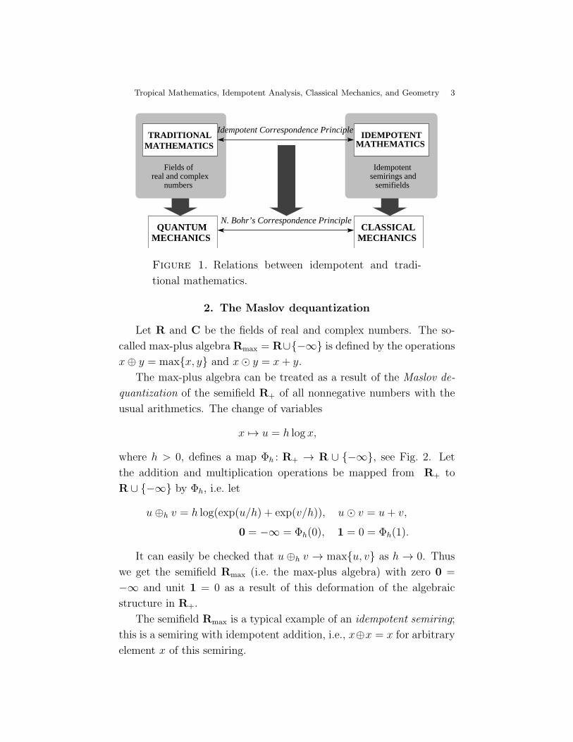
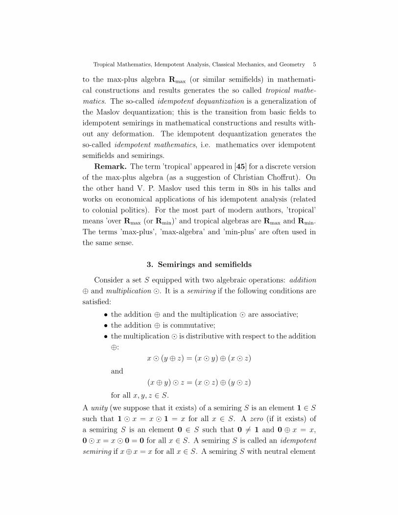
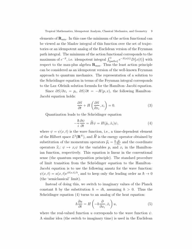
In the spirit of N. Bohr’s correspondence principle there is a (heuris-

tic) correspondence between important, useful, and interesting con-

structions and results over fields and similar results over idempotent

semirings. A systematic application of this correspondence principle

leads to a variety of theoretical and applied results [19–23], see Fig. 1.

The history of the subject is discussed, e.g., in [19]. There is a large

list of references.

Tropical Mathematics, Idempotent Analysis, Classical Mechanics, and Geometry 3

semirings andsemifields

QUANTUMMECHANICS

MATHEMATICSTRADITIONAL

numbersreal and complex

Fields of

N. Bohr’s Correspondence Principle

Idempotent Correspondence Principle

CLASSICALMECHANICS

IDEMPOTENTMATHEMATICS

Idempotent

Figure 1. Relations between idempotent and tradi-

tional mathematics.

2. The Maslov dequantization

Let R and C be the fields of real and complex numbers. The so-

called max-plus algebra Rmax = R∪{−∞} is defined by the operations

x⊕ y = max{x, y} and x⊙ y = x+ y.

The max-plus algebra can be treated as a result of the Maslov de-

quantization of the semifield R+ of all nonnegative numbers with the

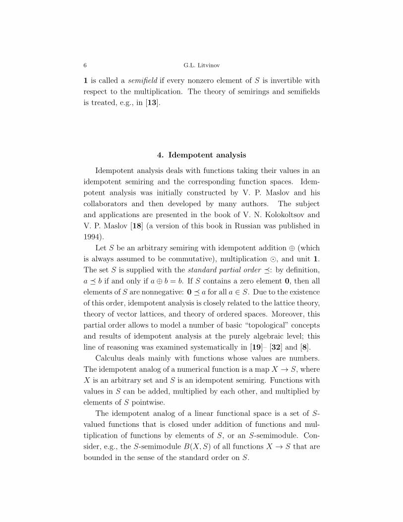
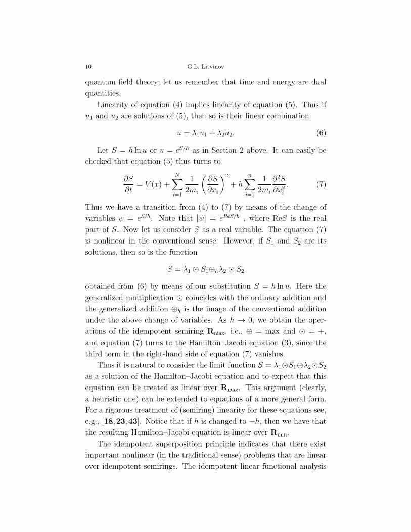
usual arithmetics. The change of variables

x 7→ u = h log x,

where h > 0, defines a map Φh : R+ → R ∪ {−∞}, see Fig. 2. Let

the addition and multiplication operations be mapped from R+ to

R ∪ {−∞} by Φh, i.e. let

u⊕h v = h log(exp(u/h) + exp(v/h)), u⊙ v = u+ v,

0 = −∞ = Φh(0), 1 = 0 = Φh(1).

It can easily be checked that u ⊕h v → max{u, v} as h → 0. Thus

we get the semifield Rmax (i.e. the max-plus algebra) with zero 0 =

−∞ and unit 1 = 0 as a result of this deformation of the algebraic

structure in R+.

The semifield Rmax is a typical example of an idempotent semiring;

this is a semiring with idempotent addition, i.e., x⊕x = x for arbitrary

element x of this semiring.

4 G.L. Litvinov

u

0 1 +RÎu

Rmax(h)

Îw

11

¥ = 0

w= lnh u

w

Figure 2. Deformation of R+ to R(h). Inset: the same

for a small value of h.

The semifield Rmax is also called a tropical algebra. The semifield

R(h) = Φh(R+) with operations ⊕h and ⊙ (i.e.+) is called a subtropical

algebra.

The semifield Rmin = R ∪ {+∞} with operations ⊕ = min and

⊙ = + (0 = +∞, 1 = 0) is isomorphic to Rmax.

The analogy with quantization is obvious; the parameter h plays

the role of the Planck constant. The map x 7→ |x| and the Maslov

dequantization for R+ give us a natural transition from the field C (or

R) to the max-plus algebra Rmax. We will also call this transition the

Maslov dequantization. In fact the Maslov dequantization corresponds

to the usual Schrodinger dequantization but for imaginary values of

the Planck constant (see below). The transition from numerical fields


to the max-plus algebra Rmax (or similar semifields) in mathemati-

cal constructions and results generates the so called tropical mathe-

matics. The so-called idempotent dequantization is a generalization of

the Maslov dequantization; this is the transition from basic fields to

idempotent semirings in mathematical constructions and results with-

out any deformation. The idempotent dequantization generates the

so-called idempotent mathematics, i.e. mathematics over idempotent

semifields and semirings.

Remark. The term ’tropical’ appeared in [45] for a discrete version

of the max-plus algebra (as a suggestion of Christian Choffrut). On

the other hand V. P. Maslov used this term in 80s in his talks and

works on economical applications of his idempotent analysis (related

to colonial politics). For the most part of modern authors, ’tropical’

means ’over Rmax (or Rmin)’ and tropical algebras are Rmax and Rmin.

The terms ’max-plus’, ’max-algebra’ and ’min-plus’ are often used in

the same sense.

3. Semirings and semifields

Consider a set S equipped with two algebraic operations: addition

⊕ and multiplication ⊙. It is a semiring if the following conditions are

satisfied:

• the addition ⊕ and the multiplication ⊙ are associative;

• the addition ⊕ is commutative;

• the multiplication⊙ is distributive with respect to the addition

⊕:

x⊙ (y ⊕ z) = (x⊙ y)⊕ (x⊙ z)

and

(x⊕ y)⊙ z = (x⊙ z)⊕ (y ⊙ z)

for all x, y, z ∈ S.

A unity (we suppose that it exists) of a semiring S is an element 1 ∈ S

such that 1 ⊙ x = x ⊙ 1 = x for all x ∈ S. A zero (if it exists) of

a semiring S is an element 0 ∈ S such that 0 6= 1 and 0 ⊕ x = x,

0⊙ x = x⊙ 0 = 0 for all x ∈ S. A semiring S is called an idempotent

semiring if x⊕ x = x for all x ∈ S. A semiring S with neutral element

6 G.L. Litvinov

1 is called a semifield if every nonzero element of S is invertible with

respect to the multiplication. The theory of semirings and semifields

is treated, e.g., in [13].

4. Idempotent analysis

Idempotent analysis deals with functions taking their values in an

idempotent semiring and the corresponding function spaces. Idem-

potent analysis was initially constructed by V. P. Maslov and his

collaborators and then developed by many authors. The subject

and applications are presented in the book of V. N. Kolokoltsov and

V. P. Maslov [18] (a version of this book in Russian was published in

1994).

Let S be an arbitrary semiring with idempotent addition ⊕ (which

is always assumed to be commutative), multiplication ⊙, and unit 1.

The set S is supplied with the standard partial order �: by definition,

a � b if and only if a⊕ b = b. If S contains a zero element 0, then all

elements of S are nonnegative: 0 � a for all a ∈ S. Due to the existence

of this order, idempotent analysis is closely related to the lattice theory,

theory of vector lattices, and theory of ordered spaces. Moreover, this

partial order allows to model a number of basic “topological” concepts

and results of idempotent analysis at the purely algebraic level; this

line of reasoning was examined systematically in [19]– [32] and [8].

Calculus deals mainly with functions whose values are numbers.

The idempotent analog of a numerical function is a map X → S, where

X is an arbitrary set and S is an idempotent semiring. Functions with

values in S can be added, multiplied by each other, and multiplied by

elements of S pointwise.

The idempotent analog of a linear functional space is a set of S-

valued functions that is closed under addition of functions and mul-

tiplication of functions by elements of S, or an S-semimodule. Con-

sider, e.g., the S-semimodule B(X,S) of all functions X → S that are

bounded in the sense of the standard order on S.


If S = Rmax, then the idempotent analog of integration is defined

by the formula

I(ϕ) =

∫ ⊕

X

ϕ(x) dx = supx∈X

ϕ(x), (1)

where ϕ ∈ B(X,S). Indeed, a Riemann sum of the form∑i

ϕ(xi) · σi

corresponds to the expression⊕i

ϕ(xi)⊙ σi = maxi

{ϕ(xi) + σi}, which

tends to the right-hand side of (1) as σi → 0. Of course, this is a purely

heuristic argument.

Formula (1) defines the idempotent (or Maslov) integral not only

for functions taking values in Rmax, but also in the general case when

any of bounded (from above) subsets of S has the least upper bound.

An idempotent (or Maslov) measure on X is defined by the formula

mψ(Y ) = supx∈Y

ψ(x), where ψ ∈ B(X,S) is a fixed function. The integral

with respect to this measure is defined by the formula

Iψ(ϕ) =

∫ ⊕

X

ϕ(x) dmψ =

∫ ⊕

X

ϕ(x)⊙ψ(x) dx = supx∈X

(ϕ(x)⊙ψ(x)). (2)

Obviously, if S = Rmin, then the standard order is opposite to the

conventional order ≤, so in this case equation (2) assumes the form∫ ⊕

X

ϕ(x) dmψ =

∫ ⊕

X

ϕ(x)⊙ ψ(x) dx = infx∈X

(ϕ(x)⊙ ψ(x)),

where inf is understood in the sense of the conventional order ≤.

5. The superposition principle and linear problems

Basic equations of quantum theory are linear; this is the superposi-

tion principle in quantum mechanics. The Hamilton–Jacobi equation,

the basic equation of classical mechanics, is nonlinear in the conven-

tional sense. However, it is linear over the semirings Rmax and Rmin.

Similarly, different versions of the Bellman equation, the basic equation

of optimization theory, are linear over suitable idempotent semirings.

This is V. P. Maslov’s idempotent superposition principle, see [36–38].

For instance, the finite-dimensional stationary Bellman equation can be

written in the form X = H⊙X⊕F , where X , H , F are matrices with

coefficients in an idempotent semiring S and the unknown matrix X is

8 G.L. Litvinov

determined by H and F [2,5,6,9,10,14,15]. In particular, standard

problems of dynamic programming and the well-known shortest path

problem correspond to the cases S = Rmax and S = Rmin, respectively.

It is known that principal optimization algorithms for finite graphs cor-

respond to standard methods for solving systems of linear equations of

this type (i.e., over semirings). Specifically, Bellman’s shortest path

algorithm corresponds to a version of Jacobi’s algorithm, Ford’s algo-

rithm corresponds to the Gauss–Seidel iterative scheme, etc. [5,6].

The linearity of the Hamilton–Jacobi equation over Rmin and Rmax,

which is the result of the Maslov dequantization of the Schrodinger

equation, is closely related to the (conventional) linearity of the Schro-

dinger equation and can be deduced from this linearity. Thus, it is

possible to borrow standard ideas and methods of linear analysis and

apply them to a new area.

Consider a classical dynamical system specified by the Hamiltonian

H = H(p, x) =

N∑

i=1

p2i2mi

+ V (x),

where x = (x1, . . . , xN) are generalized coordinates, p = (p1, . . . , pN)

are generalized momenta, mi are generalized masses, and V (x) is the

potential. In this case the Lagrangian L(x, x, t) has the form

L(x, x, t) =N∑

i=1

mix2i2

− V (x),

where x = (x1, . . . , xN), xi = dxi/dt. The value function S(x, t) of the

action functional has the form

S =

∫ t

t0

L(x(t), x(t), t) dt,

where the integration is performed along the factual trajectory of the

system. The classical equations of motion are derived as the stationar-

ity conditions for the action functional (the Hamilton principle, or the

least action principle).

For fixed values of t and t0 and arbitrary trajectories x(t), the action

functional S = S(x(t)) can be considered as a function taking the set of

curves (trajectories) to the set of real numbers which can be treated as


elements ofRmin. In this case the minimum of the action functional can

be viewed as the Maslov integral of this function over the set of trajec-

tories or an idempotent analog of the Euclidean version of the Feynman

path integral. The minimum of the action functional corresponds to the

maximum of e−S, i.e. idempotent integral∫ ⊕

{paths}e−S(x(t))D{x(t)} with

respect to the max-plus algebra Rmax. Thus the least action principle

can be considered as an idempotent version of the well-known Feynman

approach to quantum mechanics. The representation of a solution to

the Schrodinger equation in terms of the Feynman integral corresponds

to the Lax–Oleınik solution formula for the Hamilton–Jacobi equation.

Since ∂S/∂xi = pi, ∂S/∂t = −H(p, x), the following Hamilton–

Jacobi equation holds:

∂S

∂t+H

(∂S

∂xi, xi

)= 0. (3)

Quantization leads to the Schrodinger equation

−~

i

∂ψ

∂t= Hψ = H(pi, xi)ψ, (4)

where ψ = ψ(x, t) is the wave function, i.e., a time-dependent element

of the Hilbert space L2(RN), and H is the energy operator obtained by

substitution of the momentum operators pi =~

i∂∂xi

and the coordinate

operators xi : ψ 7→ xiψ for the variables pi and xi in the Hamilton-

ian function, respectively. This equation is linear in the conventional

sense (the quantum superposition principle). The standard procedure

of limit transition from the Schrodinger equation to the Hamilton–

Jacobi equation is to use the following ansatz for the wave function:

ψ(x, t) = a(x, t)eiS(x,t)/~, and to keep only the leading order as ~ → 0

(the ‘semiclassical’ limit).

Instead of doing this, we switch to imaginary values of the Planck

constant ~ by the substitution h = i~, assuming h > 0. Thus the

Schrodinger equation (4) turns to an analog of the heat equation:

h∂u

∂t= H

(−h

∂

∂xi, xi

)u, (5)

where the real-valued function u corresponds to the wave function ψ.

A similar idea (the switch to imaginary time) is used in the Euclidean

10 G.L. Litvinov

quantum field theory; let us remember that time and energy are dual

quantities.

Linearity of equation (4) implies linearity of equation (5). Thus if

u1 and u2 are solutions of (5), then so is their linear combination

u = λ1u1 + λ2u2. (6)

Let S = h ln u or u = eS/h as in Section 2 above. It can easily be

checked that equation (5) thus turns to

∂S

∂t= V (x) +

N∑

i=1

1

2mi

(∂S

∂xi

)2

+ hn∑

i=1

1

2mi

∂2S

∂x2i. (7)

Thus we have a transition from (4) to (7) by means of the change of

variables ψ = eS/h. Note that |ψ| = eReS/h , where ReS is the real

part of S. Now let us consider S as a real variable. The equation (7)

is nonlinear in the conventional sense. However, if S1 and S2 are its

solutions, then so is the function

S = λ1 ⊙ S1⊕hλ2 ⊙ S2

obtained from (6) by means of our substitution S = h ln u. Here the

generalized multiplication ⊙ coincides with the ordinary addition and

the generalized addition ⊕h is the image of the conventional addition

under the above change of variables. As h → 0, we obtain the oper-

ations of the idempotent semiring Rmax, i.e., ⊕ = max and ⊙ = +,

and equation (7) turns to the Hamilton–Jacobi equation (3), since the

third term in the right-hand side of equation (7) vanishes.

Thus it is natural to consider the limit function S = λ1⊙S1⊕λ2⊙S2

as a solution of the Hamilton–Jacobi equation and to expect that this

equation can be treated as linear over Rmax. This argument (clearly,

a heuristic one) can be extended to equations of a more general form.

For a rigorous treatment of (semiring) linearity for these equations see,

e.g., [18,23,43]. Notice that if h is changed to −h, then we have that

the resulting Hamilton–Jacobi equation is linear over Rmin.

The idempotent superposition principle indicates that there exist

important nonlinear (in the traditional sense) problems that are linear

over idempotent semirings. The idempotent linear functional analysis


(see below) is a natural tool for investigation of those nonlinear infinite-

dimensional problems that possess this property.

6. Convolution and the Fourier–Legendre transform

Let G be a group. Then the space B(G,Rmax) of all bounded func-

tions G→ Rmax (see above) is an idempotent semiring with respect to

the following analog ⊛ of the usual convolution:

(ϕ(x)⊛ ψ)(g) ==

∫ ⊕

G

ϕ(x)⊙ ψ(x−1 · g) dx = supx∈G

(ϕ(x) + ψ(x−1 · g)).

Of course, it is possible to consider other “function spaces” (and other

basic semirings instead of Rmax).

Let G = Rn, where Rn is considered as a topological group with

respect to the vector addition. The conventional Fourier–Laplace trans-

form is defined as

ϕ(x) 7→ ϕ(ξ) =

∫

G

eiξ·xϕ(x) dx, (8)

where eiξ·x is a character of the group G, i.e., a solution of the following

functional equation:

f(x+ y) = f(x)f(y).

The idempotent analog of this equation is

f(x+ y) = f(x)⊙ f(y) = f(x) + f(y),

so “continuous idempotent characters” are linear functionals of the

form x 7→ ξ · x = ξ1x1 + · · · + ξnxn. As a result, the transform in (8)

assumes the form

ϕ(x) 7→ ϕ(ξ) =

∫ ⊕

G

ξ · x⊙ ϕ(x) dx = supx∈G

(ξ · x+ ϕ(x)). (9)

The transform in (9) is nothing but the Legendre transform (up to some

notation) [38]; transforms of this kind establish the correspondence

between the Lagrangian and the Hamiltonian formulations of classical

mechanics. The Legendre transform generates an idempotent version

of harmonic analysis for the space of convex functions, see, e.g., [34].

Of course, this construction can be generalized to different classes

of groups and semirings. Transformations of this type convert the

12 G.L. Litvinov

generalized convolution ⊛ to the pointwise (generalized) multiplication

and possess analogs of some important properties of the usual Fourier

transform.

The examples discussed in this sections can be treated as fragments

of an idempotent version of the representation theory, see, e.g., [28].

In particular, “idempotent” representations of groups can be exam-

ined as representations of the corresponding convolution semirings (i.e.

idempotent group semirings) in semimodules.

7. Idempotent functional analysis

Many other idempotent analogs may be given, in particular, for

basic constructions and theorems of functional analysis. Idempotent

functional analysis is an abstract version of idempotent analysis. For

the sake of simplicity take S = Rmax and let X be an arbitrary set.

The idempotent integration can be defined by the formula (1), see

above. The functional I(ϕ) is linear over S and its values correspond to

limiting values of the corresponding analogs of Lebesgue (or Riemann)

sums. An idempotent scalar product of functions ϕ and ψ is defined

by the formula

〈ϕ, ψ〉 =

∫ ⊕

X

ϕ(x)⊙ ψ(x) dx = supx∈X

(ϕ(x)⊙ ψ(x)).

So it is natural to construct idempotent analogs of integral operators

in the form

ϕ(y) 7→ (Kϕ)(x) =

∫ ⊕

Y

K(x, y)⊙ϕ(y) dy = supy∈Y

{K(x, y)+ϕ(y)}, (10)

where ϕ(y) is an element of a space of functions defined on a set Y ,

and K(x, y) is an S-valued function on X × Y . Of course, expressions

of this type are standard in optimization problems.

Recall that the definitions and constructions described above can

be extended to the case of idempotent semirings which are condition-

ally complete in the sense of the standard order. Using the Maslov

integration, one can construct various function spaces as well as idem-

potent versions of the theory of generalized functions (distributions).

For some concrete idempotent function spaces it was proved that every


‘good’ linear operator (in the idempotent sense) can be presented in

the form (10); this is an idempotent version of the kernel theorem of

L. Schwartz; results of this type were proved by V. N. Kolokoltsov,

P. S. Dudnikov and S. N. Samborskiı, I. Singer, M. A. Shubin and

others. So every ‘good’ linear functional can be presented in the form

ϕ 7→ 〈ϕ, ψ〉, where 〈, 〉 is an idempotent scalar product.

In the framework of idempotent functional analysis results of this

type can be proved in a very general situation. In [25–28, 30, 32]

an algebraic version of the idempotent functional analysis is devel-

oped; this means that basic (topological) notions and results are sim-

ulated in purely algebraic terms (see below). The treatment covers

the subject from basic concepts and results (e.g., idempotent analogs

of the well-known theorems of Hahn-Banach, Riesz, and Riesz-Fisher)

to idempotent analogs of A. Grothendieck’s concepts and results on

topological tensor products, nuclear spaces and operators. Abstract

idempotent versions of the kernel theorem are formulated. Note

that the transition from the usual theory to idempotent functional

analysis may be very nontrivial; for example, there are many non-

isomorphic idempotent Hilbert spaces. Important results on idempo-

tent functional analysis (duality and separation theorems) were ob-

tained by G. Cohen, S. Gaubert, and J.-P. Quadrat. Idempotent

functional analysis has received much attention in the last years, see,

e.g., [1,8,14–16,40,46], [18]– [32] and works cited in [19]. Elements

of ”tropical” functional analysis are presented in [18]. All the results

presented in this section are proved in [27] (subsections 7.1 – 7.4) and

in [32] (subsections 7.5 – 7.10)

7.1. Idempotent semimodules and idempotent linear

spaces. An additive semigroup S with commutative addition ⊕ is

called an idempotent semigroup if the relation x ⊕ x = x is fulfilled

for all elements x ∈ S. If S contains a neutral element, this element

is denoted by the symbol 0. Any idempotent semigroup is a partially

ordered set with respect to the following standard order: x � y if and

only if x ⊕ y = y. It is obvious that this order is well defined and

14 G.L. Litvinov

x⊕ y = sup{x, y}. Thus, any idempotent semigroup is an upper semi-

lattice; moreover, the concepts of idempotent semigroup and upper

semilattice coincide, see [3]. An idempotent semigroup S is called a-

complete (or algebraically complete) if it is complete as an ordered set,

i.e., if any subset X in S has the least upper bound sup(X) denoted

by ⊕X and the greatest lower bound inf(X) denoted by ∧X . This

semigroup is called b-complete (or boundedly complete), if any bounded

above subset X of this semigroup (including the empty subset) has

the least upper bound ⊕X (in this case, any nonempty subset Y in

S has the greatest lower bound ∧Y and S in a lattice). Note that

any a-complete or b-complete idempotent semiring has the zero ele-

ment 0 that coincides with ⊕Ø, where Ø is the empty set. Certainly,

a-completeness implies the b-completeness. Completion by means of

cuts [3] yields an embedding S → S of an arbitrary idempotent semi-

group S into an a-complete idempotent semigroup S (which is called

a normal completion of S); in addition,S = S. The b-completion

procedure S → Sb is defined similarly: if S ∋ ∞ = supS, then Sb=S; otherwise, S = Sb ∪ {∞}. An arbitrary b-complete idempotent

semigroup S also may differ from S only by the element ∞ = supS.

Let S and T be b-complete idempotent semigroups. Then, a ho-

momorphism f : S → T is said to be a b-homomorphism if f(⊕X) =

⊕f(X) for any bounded subset X in S. If the b-homomorphism f

is extended to a homomorphism S → T of the corresponding normal

completions and f(⊕X) = ⊕f(X) for all X ⊂ S, then f is said to

be an a-homomorphism. An idempotent semigroup S equipped with a

topology such that the set {s ∈ S|s � b} is closed in this topology for

any b ∈ S is called a topological idempotent semigroup S.

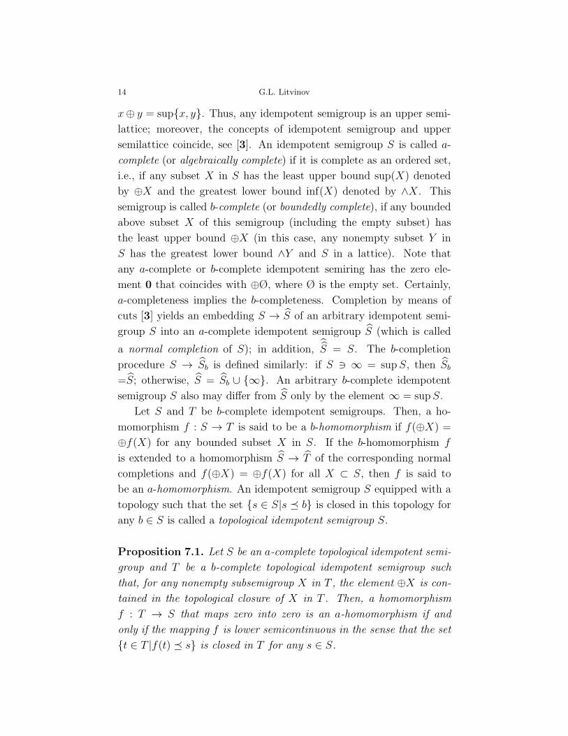
Proposition 7.1. Let S be an a-complete topological idempotent semi-

group and T be a b-complete topological idempotent semigroup such

that, for any nonempty subsemigroup X in T , the element ⊕X is con-

tained in the topological closure of X in T . Then, a homomorphism

f : T → S that maps zero into zero is an a-homomorphism if and

only if the mapping f is lower semicontinuous in the sense that the set

{t ∈ T |f(t) � s} is closed in T for any s ∈ S.


An idempotent semiring K is called a-complete (respectively b-

complete) if K is an a-complete (respectively b-complete) idempo-

tent semigroup and, for any subset (respectively, for any bounded

subset) X in K and any k ∈ K, the generalized distributive laws

k ⊙ (⊕X) = ⊕(k ⊙X) and (⊕X) ⊙ k = ⊕(X ⊙ k) are fulfilled. Gen-

eralized distributivity implies that any a-complete or b-complete idem-

potent semiring has a zero element that coincides with ⊕Ø, where Ø

is the empty set.

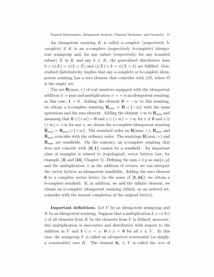
The set R(max,+) of real numbers equipped with the idempotent

addition⊕ = max and multiplication⊙ = + is an idempotent semiring;

in this case, 1 = 0. Adding the element 0 = −∞ to this semiring,

we obtain a b-complete semiring Rmax = R ∪ {−∞} with the same

operations and the zero element. Adding the element +∞ to Rmax and

assuming that 0⊙ (+∞) = 0 and x⊙ (+∞) = +∞ for x 6= 0 and x⊕

(+∞) = +∞ for any x, we obtain the a-complete idempotent semiring

Rmax = Rmax ∪ {+∞}. The standard order on R(max,+), Rmax and

Rmax coincides with the ordinary order. The semirings R(max,+) and

Rmax are semifields. On the contrary, an a-complete semiring that

does not coincide with {0, 1} cannot be a semifield. An important

class of examples is related to (topological) vector lattices (see, for

example, [3] and [44], Chapter 5). Defining the sum x⊕y as sup{x, y}

and the multiplication ⊙ as the addition of vectors, we can interpret

the vector lattices as idempotent semifields. Adding the zero element

0 to a complete vector lattice (in the sense of [3, 44]), we obtain a

b-complete semifield. If, in addition, we add the infinite element, we

obtain an a-complete idempotent semiring (which, as an ordered set,

coincides with the normal completion of the original lattice).

Important definitions. Let V be an idempotent semigroup and

K be an idempotent semiring. Suppose that a multiplication k, x 7→ k⊙

x of all elements from K by the elements from V is defined; moreover,

this multiplication is associative and distributive with respect to the

addition in V and 1 ⊙ x = x, 0 ⊙ x = 0 for all x ∈ V . In this

case, the semigroup V is called an idempotent semimodule (or simply,

a semimodule) over K. The element 0V ∈ V is called the zero of

16 G.L. Litvinov

the semimodule V if k ⊙ 0V = 0V and 0V ⊕ x = x for any k ∈ K

and x ∈ V . Let V be a semimodule over a b-complete idempotent

semiring K. This semimodule is called b-complete if it is b-complete

as an idempotent semiring and, for any bounded subsets Q in K and

X in V , the generalized distributive laws (⊕Q) ⊙ x = ⊕(Q ⊙ x) and

k ⊙ (⊕X) = ⊕(k ⊙ X) are fulfilled for all k ∈ K and x ∈ X . This

semimodule is called a-complete if it is b-complete and contains the

element ∞ = supV .

A semimodule V over a b-complete semifield K is said to be an

idempotent a-space (b-space) if this semimodule is a-complete (respec-

tively, b-complete) and the equality (∧Q) ⊙ x = ∧(Q ⊙ x) holds for

any nonempty subset Q in K and any x ∈ V , x 6= ∞ = sup V . The

normal completion V of a b-space V (as an idempotent semigroup) has

the structure of an idempotent a-space (and may differ from V only by

the element ∞ = supV ).

Let V and W be idempotent semimodules over an idempotent

semiring K. A mapping p : V → W is said to be linear (over K)

if

p(x⊕ y) = p(x)⊕ p(y) and p(k ⊙ x) = k ⊙ p(x)

for any x, y ∈ V and k ∈ K. Let the semimodules V and W be b-

complete. A linear mapping p : V → W is said to be b-linear if it

is a b-homomorphism of the idempotent semigroup; this mapping is

said to be a-linear if it can be extended to an a-homomorphism of the

normal completions V and W . Proposition 7.1 (see above) shows that

a-linearity simulates (semi)continuity for linear mappings. The normal

completion K of the semifield K is a semimodule over K. If W = K,

then the linear mapping p is called a linear functional.

Linear, a-linear and b-linear mappings are also called linear, a-linear

and b-linear operators respectively.

Examples of idempotent semimodules and spaces that are the most

important for analysis are either subsemimodules of topological vector

lattices [44] (or coincide with them) or are dual to them, i.e., consist

of linear functionals subject to some regularity condition, for exam-

ple, consist of a-linear functionals. Concrete examples of idempotent


semimodules and spaces of functions (including spaces of bounded, con-

tinuous, semicontinuous, convex, concave and Lipschitz functions) see

in [18,26,27,32] and below.

7.2. Basic results. Let V be an idempotent b-space over a b-

complete semifield K, x ∈ V . Denote by x∗ the functional V → K

defined by the formula x∗(y) = ∧{k ∈ K|y � k ⊙ x}, where y is an

arbitrary fixed element from V .

Theorem 7.2. For any x ∈ V the functional x∗ is a-linear. Any

nonzero a-linear functional f on V is given by f = x∗ for a unique

suitable element x ∈ V . If K 6= {0, 1}, then x = ⊕{y ∈ V |f(y) � 1}.

Note that results of this type obtained earlier concerning the struc-

ture of linear functionals cannot be carried over to subspaces and sub-

semimodules.

A subsemigroupW in V closed with respect to the multiplication by

an arbitrary element fromK is called a b-subspace in V if the imbedding

W → V can be extended to a b-linear mapping. The following result

is obtained from Theorem 7.2 and is the idempotent version of the

Hahn–Banach theorem.

Theorem 7.3. Any a-linear functional defined on a b-subspace W in

V can be extended to an a-linear functional on V . If x, y ∈ V and

x 6= y, then there exists an a-linear functional f on V that separates

the elements x and y, i.e., f(x) 6= f(y).

The following statements are easily derived from the definitions

and can be regarded as the analogs of the well-known results of the

traditional functional analysis (the Banach–Steinhaus and the closed-

graph theorems).

Proposition 7.4. Suppose that P is a family of a-linear mappings

of an a-space V into an a-space W and the mapping p : V → W

is the pointwise sum of the mappings of this family, i.e., p(x) =

sup{pα(x)|pα ∈ P}. Then the mapping p is a-linear.

Proposition 7.5. Let V and W be a-spaces. A linear mapping p :

V → W is a-linear if and only if its graph Γ in V ×W is closed with

18 G.L. Litvinov

respect to passing to sums (i.e., to least upper bounds) of its arbitrary

subsets.

In [8] the basic results were generalized for the case of semimodules

over the so-called reflexive b-complete semirings.

7.3. Idempotent b-semialgebras. Let K be a b-complete semi-

field and A be an idempotent b-space over K equipped with the struc-

ture of a semiring compatible with the multiplication K × A → A so

that the associativity of the multiplication is preserved. In this case,

A is called an idempotent b-semialgebra over K.

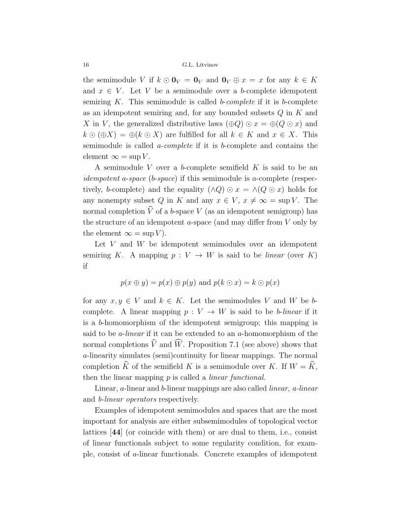
Proposition 7.6. For any invertible element x ∈ A from the b-

semialgebra A and any element y ∈ A, the equality x∗(y) = 1∗(y⊙x−1)

holds, where 1 ∈ A.

The mapping A×A→ K defined by the formula (x, y) 7→ 〈x, y〉 =

1∗(x⊙ y) is called the canonical scalar product (or simply scalar prod-

uct). The basic properties of the scalar product are easily derived from

Proposition 7.6 (in particular, the scalar product is commutative if the

b-semialgebra A is commutative). The following theorem is an idem-

potent version of the Riesz–Fisher theorem.

Theorem 7.7. Let a b-semialgebra A be a semifield. Then any nonzero

a-linear functional f on A can be represented as f(y) = 〈y, x〉, where

x ∈ A, x 6= 0 and 〈·, ·〉 is the canonical scalar product on A.

Remark 7.8. Using the completion precedures, one can extend all

the results obtained to the case of incomplete semirings, spaces, and

semimodules, see [27].

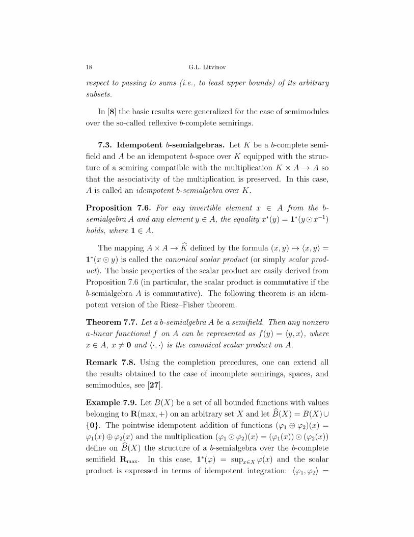
Example 7.9. Let B(X) be a set of all bounded functions with values

belonging to R(max,+) on an arbitrary set X and let B(X) = B(X)∪

{0}. The pointwise idempotent addition of functions (ϕ1 ⊕ ϕ2)(x) =

ϕ1(x)⊕ϕ2(x) and the multiplication (ϕ1 ⊙ϕ2)(x) = (ϕ1(x))⊙ (ϕ2(x))

define on B(X) the structure of a b-semialgebra over the b-complete

semifield Rmax. In this case, 1∗(ϕ) = supx∈X ϕ(x) and the scalar

product is expressed in terms of idempotent integration: 〈ϕ1, ϕ2〉 =


supx∈X(ϕ1(x)⊙ϕ2(x)) = supx∈X(ϕ1(x)+ϕ2(x)) =⊕∫X

(ϕ1(x)⊙ϕ2(x)) dx.

Scalar products of this type were systematically used in idempotent

analysis. Using Theorems 7.2 and 7.7, one can easily describe a-linear

functionals on idempotent spaces in terms of idempotent measures and

integrals.

Example 7.10. Let X be a linear space in the traditional sense.

The idempotent semiring (and linear space over R(max,+)) of con-

vex functions Conv(X,R) is b-complete but it is not a b-semialgebra

over the semifield K = R(max,+). Any nonzero a-linear functional f

on Conv(X,R) has the form

ϕ 7→ f(ϕ) = supx{ϕ(x) + ψ(x)} =

∫ ⊕

X

ϕ(x)⊙ ψ(x) dx,

where ψ is a concave function, i.e., an element of the idempotent space

Conc(X,R) = - Conv(X,R).

7.4. Linear operator, b-semimodules and subsemimodules.

In what follows, we suppose that all semigroups, semirings, semifields,

semimodules, and spaces are idempotent unless otherwise specified. We

fix a basic semiring K and examine semimodules and subsemimodules

over K. We suppose that every linear functional takes it values in the

basic semiring.

Let V and W be b-complete semimodules over a b-complete semir-

ing K. Denote by Lb(V,W ) the set of all b-linear mappings from V

to W . It is easy to check that Lb(V,W ) is an idempotent semigroup

with respect to the pointwise addition of operators; the composition

(product) of b-linear operators is also a b-linear operator, and there-

fore the set Lb(V, V ) is an idempotent semiring with respect to these

operations, see, e.g., [27]. The following proposition can be treated as

a version of the Banach–Steinhaus theorem in idempotent analysis (as

well as Proposition 7.4 above).

Proposition 7.11. Assume that S is a subset in Lb(V,W ) and the

set {g(v) | g ∈ S} is bounded in W for every element v ∈ V ; thus

the element f(v) = supg∈S g(v) exists, because the semimodule W is

20 G.L. Litvinov

b-complete. Then the mapping v 7→ f(v) is a b-linear operator, i.e., an

element of Lb(V,W ). The subset S is bounded; moreover, supS = f .

Corollary 7.12. The set Lb(V,W ) is a b-complete idempotent semi-

group with respect to the (idempotent) pointwise addition of operators.

If V = W , then Lb(V, V ) is a b-complete idempotent semiring with

respect to the operations of pointwise addition and composition of op-

erators.

Corollary 7.13. A subset S is bounded in Lb(V,W ) if and only if the

set {g(v) | g ∈ S} is bounded in the semimodule W for every element

v ∈ V .

A subset of an idempotent semimodule is called a subsemimodule

if it is closed under addition and multiplication by scalar coefficients.

A subsemimodule V of a b-complete semimodule W is b-closed if V

is closed under sums of any subsets of V that are bounded in W . A

subsemimodule of a b-complete semimodule is called a b-subsemimodule

if the corresponding embedding is a b-homomorphism. It is easy to

see that each b-closed subsemimodule is a b-subsemimodule, but the

converse is not true. The main feature of b-subsemimodules is that

restrictions of b-linear operators and functionals to these semimodules

are b-linear.

The following definitions are very important for our purposes. As-

sume that W is an idempotent b-complete semimodule over a b-

complete idempotent semiring K and V is a subset of W such that

V is closed under multiplication by scalar coefficients and is an upper

semilattice with respect to the order induced from W . Let us define

an addition operation in V by the formula x ⊕ y = sup{x, y}, where

sup means the least upper bound in V . If K is a semifield, then V is

a semimodule over K with respect to this addition.

For an arbitrary b-complete semiring K, we will say that V is a

quasisubsemimodule of W if V is a semimodule with respect to this

addition (this means that the corresponding distribution laws hold).

Recall that the simbol ∧ means the greatest lower bound (see

Subsection 7.1 above). A quasisubsemimodule V of an idempotent


b-complete semimodule W is called a ∧-subsemimodule if it contains

0 and is closed under the operations of taking infima (greatest lower

bounds) in W . It is easy to check that each ∧-subsemimodule is a

b-complete semimodule.

Note that quasisubsemimodules and ∧-subsemimodules may fail to

be subsemimodules, because only the order is induced and not the

corresponding addition (see Example 7.18 below).

Recall that idempotent semimodules over semifields are idempo-

tent spaces. In idempotent mathematics, such spaces are analogs of

traditional linear (vector) spaces over fields. In a similar way we use

the corresponding terms like b-spaces, b-subspaces, b-closed subspaces,

∧-subspaces, etc.

Some examples are presented below.

7.5. Functional semimodules. Let X be an arbitrary nonempty

set and K be an idempotent semiring. By K(X) denote the semimod-

ule of all mappings (functions) X → K endowed with the pointwise

operations. By Kb(X) denote the subsemimodule of K(X) consist-

ing of all bounded mappings. If K is a b-complete semiring, then

K(X) and Kb(X) are b-complete semimodules. Note that Kb(X) is a

b-subsemimodule but not a b-closed subsemimodule of K(X). Given a

point x ∈ X , by δx denote the functional onK(X) that maps f to f(x).

It can easily be checked that the functional δx is b-linear on K(X).

We say that a quasisubsemimodule of K(X) is an (idempotent)

functional semimodule on the set X . An idempotent functional semi-

module in K(X) is called b-complete if it is a b-complete semimodule.

A functional semimodule V ⊂ K(X) is called a functional b-

semimodule if it is a b-subsemimodule of K(X); a functional semi-

module V ⊂ K(X) is called a functional ∧-semimodule if it is a ∧-

subsemimodule of K(X).

In general, a functional of the form δx on a functional semimodule is

not even linear, much less b-linear (see Example 7.18 below). However,

the following proposition holds, which is a direct consequence of our

definitions.

22 G.L. Litvinov

Proposition 7.14. An arbitrary b-complete functional semimodule W

on a set X is a b-subsemimodule of K(X) if and only if each functional

of the form δx (where x ∈ X) is b-linear on W .

Example 7.15. The semimodule Kb(X) (consisting of all bounded

mappings from an arbitrary set X to a b-complete idempotent semiring

K) is a functional ∧-semimodule. Hence it is a b-complete semimodule

over K. Moreover, Kb(X) is a b-subsemimodule of the semimodule

K(X) consisting of all mappings X → K.

Example 7.16. If X is a finite set consisting of n elements (n > 0),

then Kb(X) = K(X) is an “n-dimensional” semimodule over K; it is

denoted by Kn. In particular, Rnmax is an idempotent space over the

semifield Rmax, and Rnmax is a semimodule over the semiring Rmax.

Note that Rnmax can be treated as a space over the semifield Rmax. For

example, the semiring Rmax can be treated as a space (semimodule)

over Rmax.

Example 7.17. Let X be a topological space. Denote by USC(X)

the set of all upper semicontinuous functions with values in Rmax. By

definition, a function f(x) is upper semicontinuous if the set Xs = {x ∈

X | f(x) ≥ s} is closed in X for every element s ∈ Rmax (see, e.g.,

[27], Sec. 2.8). If a family {fα} consists of upper semicontinuous (e.g.,

continuous) functions and f(x) = infα fα(x), then f(x) ∈ USC(X). It

is easy to check that USC(X) has a natural structure of an idempotent

space over Rmax. Moreover, USC(X) is a functional ∧-space on X and

a b-space. The subspace USC(X) ∩Kb(X) of USC(X) consisting of

bounded (from above) functions has the same properties.

Example 7.18. Note that an idempotent functional semimodule (and

even a functional ∧-semimodule) on a set X is not necessarily a sub-

semimodule of K(X). The simplest example is the functional space

(over K = Rmax) Conc(R) consisting of all concave functions on R

with values in Rmax. Recall that a function f belongs to Conc(R) if

and only if the subgraph of this function is convex, i.e., the formula

f(ax + (1 − a)y) ≥ af(x) + (1 − a)f(y) is valid for 0 ≤ a ≤ 1. The

basic operations with 0 ∈ Rmax can be defined in an obvious way. If


f, g ∈Conc(R), then denote by f ⊕ g the sum of these functions in

Conc(R). The subgraph of f ⊕ g is the convex hull of the subgraphs

of f and g. Thus f ⊕ g does not coincide with the pointwise sum (i.e.,

max{f(x), g(x)}).

Example 7.19. Let X be a nonempty metric space with a fixed metric

r. Denote by Lip(X) the set of all functions defined on X with values

in Rmax satisfying the following Lipschitz condition:

| f(x)⊙ (f(y))−1 |=| f(x)− f(y) |≤ r(x, y),

where x, y are arbitrary elements of X . The set Lip(X) consists of

continuous real-valued functions (but not all of them!) and (by def-

inition) the function equal to −∞ = 0 at every point x ∈ X . The

set Lip(X) has the structure of an idempotent space over the semifield

Rmax. Spaces of the form Lip(X) are said to be Lipschitz spaces. These

spaces are b-subsemimodules in K(X).

7.6. Integral representations of linear operators in func-

tional semimodules. Let W be an idempotent b-complete semimod-

ule over a b-complete semiring K and V ⊂ K(X) be a b-complete

functional semimodule on X . A mapping A : V → W is called an

integral operator or an operator with an integral representation if there

exists a mapping k : X → W , called the integral kernel (or kernel) of

the operator A, such that

Af = supx∈X

(f(x)⊙ k(x)). (11)

In idempotent analysis, the right-hand side of formula (11) is often

written as∫ ⊕

Xf(x) ⊙ k(x)dx. Regarding the kernel k, it is assumed

that the set {f(x) ⊙ k(x)|x ∈ X} is bounded in W for all f ∈ V

and x ∈ X . We denote the set of all functions with this property

by kernV,W (X). In particular, if W = K and A is a functional, then

this functional is called integral. Thus each integral functional can be

presented in the form of a “scalar product” f 7→∫ ⊕

Xf(x) ⊙ k(x) dx,

where k(x) ∈ K(X); in idempotent analysis, this situation is standard.

24 G.L. Litvinov

Note that a functional of the form δy (where y ∈ X) is a typical

integral functional; in this case, k(x) = 1 if x = y and k(x) = 0

otherwise.

We call a functional semimodule V ⊂ K(X) nondegenerate if for

every point x ∈ X there exists a function g ∈ V such that g(x) = 1,

and admissible if for every function f ∈ V and every point x ∈ X

such that f(x) 6= 0 there exists a function g ∈ V such that g(x) = 1

and f(x)⊙ g < f .

Note that all idempotent functional semimodules over semifields are

admissible (it is sufficient to set g = f(x)−1 ⊙ f).

Proposition 7.20. Denote by XV the subset of X defined by the for-

mula XV = {x ∈ X | ∃f ∈ V : f(x) = 1}. If the semimod-

ule V is admissible, then the restriction to XV defines an embedding

i : V → K(XV ) and its image i(V ) is admissible and nondegenerate.

If a mapping k : X → W is a kernel of a mapping A : V → W ,

then the mapping kV : X → W that is equal to k on XV and equal to

0 on X r XV is also a kernel of A.

A mapping A : V → W is integral if and only if the mapping

i−1A : i(A) →W is integral.

In what follows, K always denotes a fixed b-complete idempotent

(basic) semiring. If an operator has an integral representation, this

representation may not be unique. However, if the semimodule V is

nondegenerate, then the set of all kernels of a fixed integral operator

is bounded with respect to the natural order in the set of all kernels

and is closed under the supremum operation applied to its arbitrary

subsets. In particular, any integral operator defined on a nondegenerate

functional semimodule has a unique maximal kernel.

An important point is that an integral operator is not necessarily

b-linear and even linear except when V is a b-subsemimodule of K(X)

(see Proposition 7.21 below).

If W is a functional semimodule on a nonempty set Y , then an

integral kernel k of an operator A can be naturally identified with

the function on X × Y defined by the formula k(x, y) = (k(x))(y).

This function will also be called an integral kernel (or kernel) of the


operator A. As a result, the set kernV,W (X) is identified with the set

kernV,W (X, Y ) of all mappings k : X × Y → K such that for every

point x ∈ X the mapping kx : y 7→ k(x, y) lies in W and for every

v ∈ V the set {v(x) ⊙ kx|x ∈ X} is bounded in W . Accordingly,

the set of all integral kernels of b-linear operators can be embedded

into kernV,W (X, Y ).

If V andW are functional b-semimodules on X and Y , respectively,

then the set of all kernels of b-linear operators can be identified with

kernV,W (X, Y ) and the following formula holds:

Af(y) = supx∈X

(f(x)⊙ k(x, y)) =

∫ ⊕

X

f(x)⊙ k(x, y)dx. (12)

This formula coincides with the usual definition of an integral repre-

sentation of an operator. Note that formula (11) can be rewritten in

the form

Af = supx∈X

(δx(f)⊙ k(x)). (13)

Proposition 7.21. An arbitrary b-complete functional semimodule V

on a nonempty set X is a functional b-semimodule on X (i.e., a b-sub-

semimodule of K(X)) if and only if all integral operators defined on V

are b-linear.

The following notion (definition) is especially important for our

purposes. Let V ⊂ K(X) be a b-complete functional semimodule over

a b-complete idempotent semiring K. We say that the kernel theorem

holds for the semimodule V if every b-linear mapping from V into an

arbitrary b-complete semimodule overK has an integral representation.

Theorem 7.22. Assume that a b-complete semimodule W over a

b-complete semiring K and an admissible functional ∧-semimodule

V ⊂ K(X) are given. Then every b-linear operator A : V → W

has an integral representation of the form (11). In particular, if W

is a functional b-semimodule on a set Y , then the operator A has an

integral representation of the form (12). Thus for the semimodule V

the kernel theorem holds.

26 G.L. Litvinov

Remark 7.23. Examples of admissible functional ∧-semimodules (and

∧-spaces) appearing in Theorem 7.22 are presented above, see, e.g., ex-

amples 7.15 –7.17. Thus for these functional semimodules and spaces

V over K, the kernel theorem holds and every b-linear mapping V into

an arbitrary b-complete semimodule W over K has an integral repre-

sentation (12). Recall that every functional space over a b-complete

semifield is admissible, see above.

7.7. Nuclear operators and their integral representations.

Let us introduce some important definitions. Assume that V and W

are b-complete semimodules. A mapping g : V → W is called one-

dimensional (or a mapping of rank 1) if it is of the form v 7→ φ(v)⊙w,

where φ is a b-linear functional on V and w ∈ W . A mapping g is

called b-nuclear if it is the sum (i.e., supremum) of a bounded set of

one-dimensional mappings. Since every one-dimensional mapping is b-

linear (because the functional φ is b-linear), every b-nuclear operator is

b-linear (see Corollary 7.12 above). Of course, b-nuclear mappings are

closely related to tensor products of idempotent semimodules, see [26].

By φ ⊙ w we denote the one-dimensional operator v 7→ φ(v) ⊙ w.

In fact, this is an element of the corresponding tensor product.

Proposition 7.24. The composition (product) of a b-nuclear and a b-

linear mapping or of a b-linear and a b-nuclear mapping is a b-nuclear

operator.

Theorem 7.25. Assume that W is a b-complete semimodule over a

b-complete semiring K and V ⊂ K(X) is a functional b-semimodule.

If every b-linear functional on V is integral, then a b-linear operator

A : V → W has an integral representation if and only if it is b-nuclear.

7.8. The b-approximation property and b-nuclear semi-

modules and spaces. We say that a b-complete semimodule V has

the b-approximation property if the identity operator id:V → V is b-

nuclear (for a treatment of the approximation property for locally con-

vex spaces in the traditional functional analysis, see [44]).


Let V be an arbitrary b-complete semimodule over a b-complete

idempotent semiring K. We call this semimodule a b-nuclear semimod-

ule if any b-linear mapping of V to an arbitrary b-complete semimodule

W over K is a b-nuclear operator. Recall that, in the traditional func-

tional analysis, a locally convex space is nuclear if and only if all con-

tinuous linear mappings of this space to any Banach space are nuclear

operators, see [44].

Proposition 7.26. Let V be an arbitrary b-complete semimodule over

a b-complete semiring K. The following statements are equivalent:

1) the semimodule V has the b-approximation property;

2) every b-linear mapping from V to an arbitrary b-complete semimod-

ule W over K is b-nuclear;

3) every b-linear mapping from an arbitrary b-complete semimodule W

over K to the semimodule V is b-nuclear.

Corollary 7.27. An arbitrary b-complete semimodule over a b-

complete semiring K is b-nuclear if and only if this semimodule has

the b-approximation property.

Recall that, in the traditional functional analysis, any nuclear space

has the approximation property but the converse is not true.

Concrete examples of b-nuclear spaces and semimodules are de-

scribed in Examples 7.15, 7.16 and 7.19 (see above). Important b-

nuclear spaces and semimodules (e.g., the so-called Lipschitz spaces

and semi-Lipschitz semimodules) are described in [32]. In this paper

there is a description of all functional b-semimodules for which the ker-

nel theorem holds (as semi-Lipschitz semimodules); this result is due

to G. B. Shpiz.

It is easy to show that the idempotent spaces USC(X) and Conc(R)

(see Examples 7.17 and 7.18) are not b-nuclear (however, for these

spaces the kernel theorem is true). The reason is that these spaces

are not functional b-spaces and the corresponding δ-functionals are not

b-linear (and even linear).

28 G.L. Litvinov

7.9. Kernel theorems for functional b-semimodules. Let

V ⊂ K(X) be a b-complete functional semimodule over a b-complete

semiring K. Recall that for V the kernel theorem holds if every b-linear

mapping of this semimodule to an arbitrary b-complete semimodule

over K has an integral representation.

Theorem 7.28. Assume that a b-complete semiringK and a nonempty

set X are given. The kernel theorem holds for any functional b-

semimodule V ⊂ K(X) if and only if every b-linear functional on

V is integral and the semimodule V is b-nuclear, i.e., has the b-

approximation property.

Corollary 7.29. If for a functional b-semimodule the kernel theorem

holds, then this semimodule is b-nuclear.

Note that the possibility to obtain an integral representation of a

functional means that one can decompose it into a sum of functionals

of the form δx.

Corollary 7.30. Assume that a b-complete semiring K and a

nonempty set X are given. The kernel theorem holds for a functional

b-semimodule V ⊂ K(X) if and only if the identity operator id: V → V

is integral.

7.10. Integral representations of operators in abstract

idempotent semimodules. In this subsection, we examine the fol-

lowing problem: when a b-complete idempotent semimodule V over a

b-complete semiring is isomorphic to a functional b-semimoduleW such

that the kernel theorem holds for W .

Assume that V is a b-complete idempotent semimodule over a b-

complete semiring K and φ is a b-linear functional defined on V . We

call this functional a δ-functional if there exists an element v ∈ V such

that

φ(w)⊙ v < w

for every element w ∈ V . It is easy to see that every functional of the

form δx is a δ-functional in this sense (but the converse is not true in

general).


Denote by ∆(V ) the set of all δ-functionals on V . Denote by i∆ the

natural mapping V → K(∆(V )) defined by the formula

(i∆(v))(φ) = φ(v)

for all φ ∈ ∆(V ). We say that an element v ∈ V is pointlike if there

exists a b-linear functional φ such that φ(w) ⊙ v < w for all w ∈ V .

The set of all pointlike elements of V will be denoted by P (V ). Recall

that by φ⊙ v we denote the one-dimensional operator w 7→ φ(w)⊙ v.

The following assertion is an obvious consequence of our definitions

(including the definition of the standard order) and the idempotency

of our addition.

Remark 7.31. If a one-dimensional operator φ⊙ v appears in the de-

composition of the identity operator on V into a sum of one-dimensional

operators, then φ ∈ ∆(V ) and v ∈ P (V ).

Denote by id and Id the identity operators on V and i∆(V ), re-

spectively.

Proposition 7.32. If the operator id is b-nuclear, then i∆ is an em-

bedding and the operator Id is integral.

If the operator i∆ is an embedding and the operator Id is integral,

then the operator id is b-nuclear.

Theorem 7.33. A b-complete idempotent semimodule V over a b-

complete idempotent semiring K is isomorphic to a functional b-

semimodule for which the kernel theorem holds if and only if the identity

mapping on V is a b-nuclear operator, i.e., V is a b-nuclear semimod-

ule.

The following proposition shows that, in a certain sense, the em-

bedding i∆ is a universal representation of a b-nuclear semimodule in

the form of a functional b-semimodule for which the kernel theorem

holds.

Proposition 7.34. Let K be a b-complete idempotent semiring, X be

a nonempty set, and V ⊂ K(X) be a functional b-semimodule on X for

which the kernel theorem holds. Then there exists a natural mapping

30 G.L. Litvinov

i : X → ∆(V ) such that the corresponding mapping i∗ : K(∆(V )) →

K(X) is an isomorphism of i∆(V ) onto V .

8. The dequantization transform, convex geometry and the

Newton polytopes

Let X be a topological space. For functions f(x) defined on X we

shall say that a certain property is valid almost everywhere (a.e.) if

it is valid for all elements x of an open dense subset of X . Suppose

X is Cn or Rn; denote by Rn+ the set x = { (x1, . . . , xn) ∈ X | xi ≥

0 for i = 1, 2, . . . , n. For x = (x1, . . . , xn) ∈ X we set exp(x) =

(exp(x1), . . . , exp(xn)); so if x ∈ Rn, then exp(x) ∈ Rn+.

Denote by F(Cn) the set of all functions defined and continuous

on an open dense subset U ⊂ Cn such that U ⊃ Rn+. It is clear that

F(Cn) is a ring (and an algebra over C) with respect to the usual

addition and multiplications of functions.

For f ∈ F(Cn) let us define the function fh by the following for-

mula:

fh(x) = h log |f(exp(x/h))|, (14)

where h is a (small) real positive parameter and x ∈ Rn. Set

f(x) = limh→+0

fh(x), (15)

if the right-hand side of (15) exists almost everywhere.

We shall say that the function f(x) is a dequantization of the func-

tion f(x) and the map f(x) 7→ f(x) is a dequantization transform. By

construction, fh(x) and f(x) can be treated as functions taking their

values in Rmax. Note that in fact fh(x) and f(x) depend on the re-

striction of f to Rn+ only; so in fact the dequantization transform is

constructed for functions defined on Rn+ only. It is clear that the de-

quantization transform is generated by the Maslov dequantization and

the map x 7→ |x|.

Of course, similar definitions can be given for functions defined on

Rn and Rn+. If s = 1/h, then we have the following version of (14) and

(15):

f(x) = lims→∞

(1/s) log |f(esx)|. (15′)


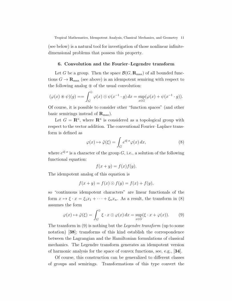
α β

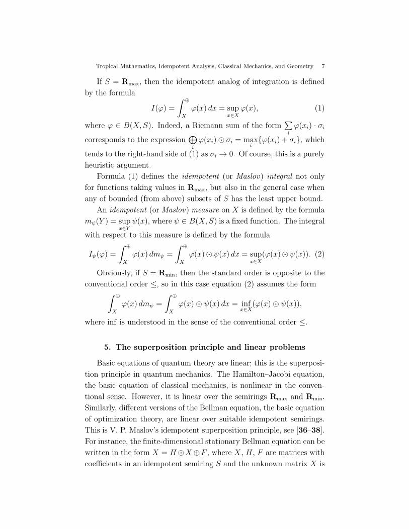
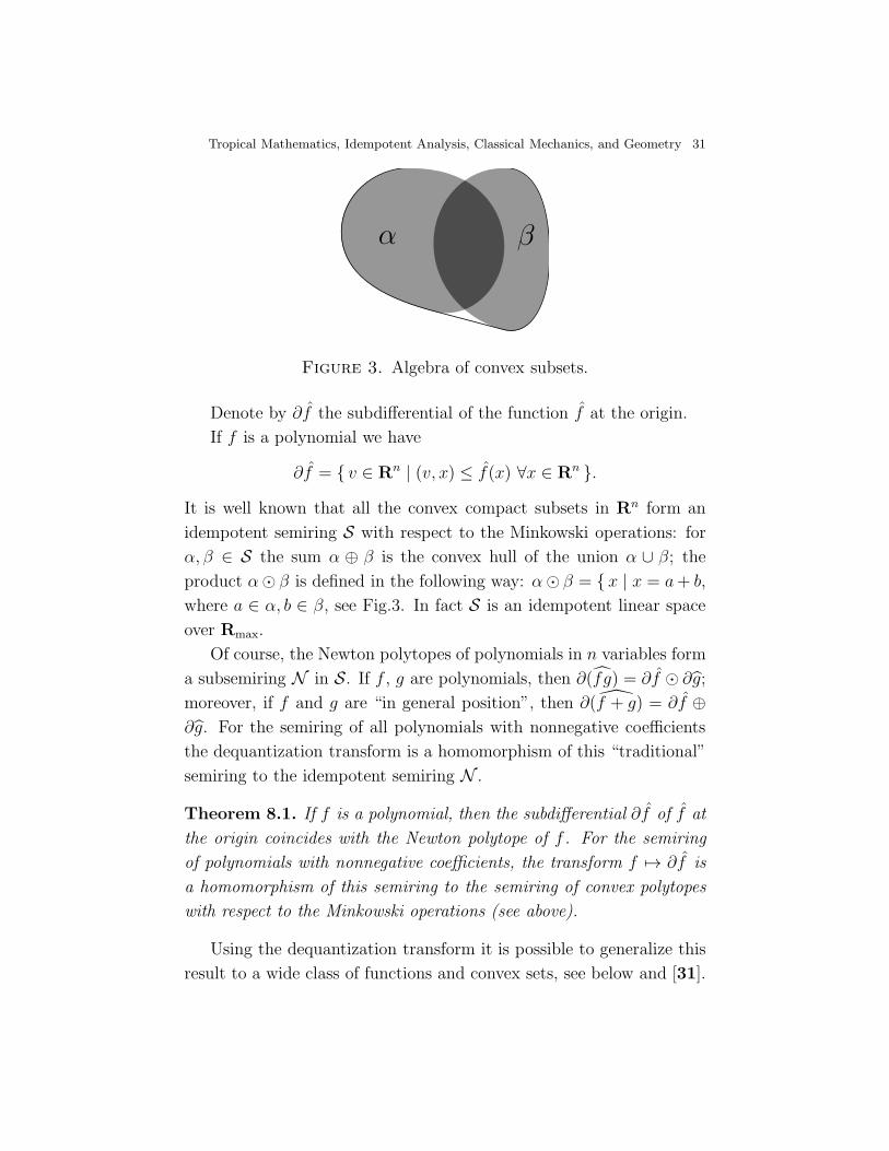
Figure 3. Algebra of convex subsets.

Denote by ∂f the subdifferential of the function f at the origin.

If f is a polynomial we have

∂f = { v ∈ Rn | (v, x) ≤ f(x) ∀x ∈ Rn }.

It is well known that all the convex compact subsets in Rn form an

idempotent semiring S with respect to the Minkowski operations: for

α, β ∈ S the sum α ⊕ β is the convex hull of the union α ∪ β; the

product α⊙ β is defined in the following way: α⊙ β = { x | x = a+ b,

where a ∈ α, b ∈ β, see Fig.3. In fact S is an idempotent linear space

over Rmax.

Of course, the Newton polytopes of polynomials in n variables form

a subsemiring N in S. If f , g are polynomials, then ∂(f g) = ∂f ⊙ ∂g;

moreover, if f and g are “in general position”, then ∂(f + g) = ∂f ⊕

∂g. For the semiring of all polynomials with nonnegative coefficients

the dequantization transform is a homomorphism of this “traditional”

semiring to the idempotent semiring N .

Theorem 8.1. If f is a polynomial, then the subdifferential ∂f of f at

the origin coincides with the Newton polytope of f . For the semiring

of polynomials with nonnegative coefficients, the transform f 7→ ∂f is

a homomorphism of this semiring to the semiring of convex polytopes

with respect to the Minkowski operations (see above).

Using the dequantization transform it is possible to generalize this

result to a wide class of functions and convex sets, see below and [31].

32 G.L. Litvinov

8.1. Dequantization transform: algebraic properties. De-

note by V the set Rn treated as a linear Euclidean space (with the

scalar product (x, y) = x1y1 + x2y2 + · · · + xnyn) and set V+ = Rn+.

We shall say that a function f ∈ F(Cn) is dequantizable whenever its

dequantization f(x) exists (and is defined on an open dense subset of

V ). By D(Cn) denote the set of all dequantizable functions and by

D(V ) denote the set { f | f ∈ D(Cn) }. Recall that functions from

D(Cn) (and D(V )) are defined almost everywhere and f = g means

that f(x) = g(x) a.e., i.e., for x ranging over an open dense subset of

Cn (resp., of V ). Denote by D+(Cn) the set of all functions f ∈ D(Cn)

such that f(x1, . . . , xn) ≥ 0 if xi ≥ 0 for i = 1, . . . , n; so f ∈ D+(Cn) if

the restriction of f to V+ = Rn+ is a nonnegative function. By D+(V )

denote the image of D+(Cn) under the dequantization transform. We

shall say that functions f, g ∈ D(Cn) are in general position whenever

f(x) 6= g(x) for x running an open dense subset of V .

Theorem 8.2. For functions f, g ∈ D(Cn) and any nonzero constant

c, the following equations are valid:

1) f g = f + g;

2) |f | = f ; cf = f ; c = 0;

3) (f + g)(x) = max{f(x), g(x)} a.e. if f and g are nonnegative

on V+ (i.e., f, g ∈ D+(Cn)) or f and g are in general position.

Left-hand sides of these equations are well-defined automatically.

Corollary 8.3. The set D+(Cn) has a natural structure of a semir-

ing with respect to the usual addition and multiplication of functions

taking their values in C. The set D+(V ) has a natural structure of

an idempotent semiring with respect to the operations (f ⊕ g)(x) =

max{f(x), g(x)}, (f ⊙ g)(x) = f(x) + g(x); elements of D+(V ) can be

naturally treated as functions taking their values in Rmax. The dequan-

tization transform generates a homomorphism from D+(Cn) to D+(V ).

8.2. Generalized polynomials and simple functions. For any

nonzero number a ∈ C and any vector d = (d1, . . . , dn) ∈ V = Rn we

set ma,d(x) = a∏n

i=1 xdii ; functions of this kind we shall call general-

ized monomials. Generalized monomials are defined a.e. on Cn and on


V+, but not on V unless the numbers di take integer or suitable ratio-

nal values. We shall say that a function f is a generalized polynomial

whenever it is a finite sum of linearly independent generalized mono-

mials. For instance, Laurent polynomials and Puiseax polynomials are

examples of generalized polynomials.

As usual, for x, y ∈ V we set (x, y) = x1y1 + · · · + xnyn. The

following proposition is a result of a trivial calculation.

Proposition 8.4. For any nonzero number a ∈ V = C and any vector

d ∈ V = Rn we have (ma,d)h(x) = (d, x) + h log |a|.

Corollary 8.5. If f is a generalized monomial, then f is a linear

function.

Recall that a real function p defined on V = Rn is sublinear if

p = supα pα, where {pα} is a collection of linear functions. Sublinear

functions defined everywhere on V = Rn are convex; thus these func-

tions are continuous, see [34]. We discuss sublinear functions of this

kind only. Suppose p is a continuous function defined on V , then p is

sublinear whenever

1) p(x+ y) ≤ p(x) + p(y) for all x, y ∈ V ;

2) p(cx) = cp(x) for all x ∈ V , c ∈ R+.

So if p1, p2 are sublinear functions, then p1 + p2 is a sublinear

function.

We shall say that a function f ∈ F(Cn) is simple, if its dequanti-

zation f exists and a.e. coincides with a sublinear function; by misuse

of language, we shall denote this (uniquely defined everywhere on V )

sublinear function by the same symbol f .

Recall that simple functions f and g are in general position if

f(x) 6= g(x) for all x belonging to an open dense subset of V . In par-

ticular, generalized monomials are in general position whenever they

are linearly independent.

Denote by Sim(Cn) the set of all simple functions defined on V

and denote by Sim+(Cn) the set Sim(Cn) ∩ D+(C

n). By Sbl(V ) de-

note the set of all (continuous) sublinear functions defined on V = Rn

and by Sbl+(V ) denote the image Sim+(Cn) of Sim+(C

n) under the

dequantization transform.

34 G.L. Litvinov

The following statements can be easily deduced from Theorem 8.2

and definitions.

Corollary 8.6. The set Sim+(Cn) is a subsemiring of D+(C

n) and

Sbl+(V ) is an idempotent subsemiring of D+(V ). The dequantization

transform generates an epimorphism of Sim+(Cn) onto Sbl+(V ). The

set Sbl(V ) is an idempotent semiring with respect to the operations

(f ⊕ g)(x) = max{f(x), g(x)}, (f ⊙ g)(x) = f(x) + g(x).

Corollary 8.7. Polynomials and generalized polynomials are simple

functions.

We shall say that functions f, g ∈ D(V ) are asymptotically equiva-

lent whenever f = g; any simple function f is an asymptotic monomial

whenever f is a linear function. A simple function f will be called

an asymptotic polynomial whenever f is a sum of a finite collection of

nonequivalent asymptotic monomials.

Corollary 8.8. Every asymptotic polynomial is a simple function.

Example 8.9. Generalized polynomials, logarithmic functions of (gen-

eralized) polynomials, and products of polynomials and logarithmic

functions are asymptotic polynomials. This follows from our defini-

tions and formula (15).

8.3. Subdifferentials of sublinear functions. We shall use

some elementary results from convex analysis. These results can be

found, e.g., in [34], ch. 1, §1.

For any function p ∈ Sbl(V ) we set

∂p = { v ∈ V | (v, x) ≤ p(x) ∀x ∈ V }.

It is well known from convex analysis that for any sublinear func-

tion p the set ∂p is exactly the subdifferential of p at the origin. The

following propositions are also known in convex analysis.

Proposition 8.10. Suppose p1, p2 ∈ Sbl(V ), then

1) ∂(p1 + p2) = ∂p1 ⊙ ∂p2 = { v ∈ V | v = v1 +

v2, where v1 ∈ ∂p1, v2 ∈ ∂p2 };


2) ∂(max{p1(x), p2(x)}) = ∂p1 ⊕ ∂p2.

Recall that ∂p1 ⊕ ∂p2 is a convex hull of the set ∂p1 ∪ ∂p2.

Proposition 8.11. Suppose p ∈ Sbl(V ). Then ∂p is a nonempty con-

vex compact subset of V .

Corollary 8.12. The map p 7→ ∂p is a homomorphism of the idempo-

tent semiring Sbl(V ) (see Corollary 8.3) to the idempotent semiring S

of all convex compact subsets of V (see Subsection 8.1 above).

8.4. Newton sets for simple functions. For any simple func-

tion f ∈ Sim(Cn) let us denote by N(f) the set ∂(f ). We shall call

N(f) the Newton set of the function f .

Proposition 8.13. For any simple function f , its Newton set N(f) is

a nonempty convex compact subset of V .

This proposition follows from Proposition 8.11 and definitions.

Theorem 8.14. Suppose that f and g are simple functions. Then

1) N(fg) = N(f) ⊙ N(g) = { v ∈ V | v = v1 + v2 with v1 ∈

N(f), v2 ∈ N(g);

2) N(f + g) = N(f)⊕N(g), if f1 and f2 are in general position

or f1, f2 ∈ Sim+(Cn) (recall that N(f) ⊕ N(g) is the convex

hull of N(f) ∪N(g)).

This theorem follows from Theorem 8.2, Proposition 8.10 and defi-

nitions.

Corollary 8.15. The map f 7→ N(f) generates a homomorphism from

Sim+(Cn) to S.

Proposition 8.16. Let f = ma,d(x) = a∏n

i=1 xdii be a monomial; here

d = (d1, . . . , dn) ∈ V = Rn and a is a nonzero complex number. Then

N(f) = {d}.

This follows from Proposition 8.4, Corollary 8.5 and definitions.

Corollary 8.17. Let f =∑

d∈Dmad,d be a polynomial. Then N(f) is

the polytope ⊕d∈D{d}, i.e. the convex hull of the finite set D.

36 G.L. Litvinov

This statement follows from Theorem 8.14 and Proposition 8.16.

Thus in this case N(f) is the well-known classical Newton polytope of

the polynomial f .

Now the following corollary is obvious.

Corollary 8.18. Let f be a generalized or asymptotic polynomial.

Then its Newton set N(f) is a convex polytope.

Example 8.19. Consider the one dimensional case, i.e., V = R and

suppose f1 = anxn + an−1x

n−1 + · · ·+ a0 and f2 = bmxm+ bm−1x

m−1 +

· · · + b0, where an 6= 0, bm 6= 0, a0 6= 0, b0 6= 0. Then N(f1) is the

segment [0, n] and N(f2) is the segment [0, m]. So the map f 7→ N(f)

corresponds to the map f 7→ deg(f), where deg(f) is a degree of the

polynomial f . In this case Theorem 2 means that deg(fg) = deg f +

deg g and deg(f + g) = max{deg f, deg g} = max{n,m} if ai ≥ 0,

bi ≥ 0 or f and g are in general position.

9. Dequantization of set functions and measures on metric

spaces

The following results are presented in [33].

Example 9.1. Let M be a metric space, S its arbitrary subset with a

compact closure. It is well-known that a Euclidean d-dimensional ball

Bρ of radius ρ has volume

vold(Bρ) =Γ(1/2)d

Γ(1 + d/2)ρd,

where d is a natural parameter. By means of this formula it is possible

to define a volume of Bρ for any real d. Cover S by a finite number of

balls of radii ρm. Set

vd(S) := limρ→0

infρm<ρ

∑

m

vold(Bρm).

Then there exists a number D such that vd(S) = 0 for d > D and

vd(S) = ∞ for d < D. This number D is called the Hausdorff-

Besicovich dimension (or HB-dimension) of S, see, e.g., [35]. Note


that a set of non-integral HB-dimension is called a fractal in the sense

of B. Mandelbrot.

Theorem 9.2. Denote by Nρ(S) the minimal number of balls of radius

ρ covering S. Then

D(S) = limρ→+0

logρ(Nρ(S)−1),

where D(S) is the HB-dimension of S. Set ρ = e−s, then

D(S) = lims→+∞

(1/s) · logNexp(−s)(S).

So the HB-dimensionD(S) can be treated as a result of a dequantization

of the set function Nρ(S).

Example 9.3. Let µ be a set function on M (e.g., a probability mea-

sure) and suppose that µ(Bρ) < ∞ for every ball Bρ. Let Bx,ρ be a

ball of radius ρ having the point x ∈ M as its center. Then define

µx(ρ) := µ(Bx,ρ) and let ρ = e−s and

Dx,µ := lims→+∞

−(1/s) · log(|µx(e−s)|).

This number could be treated as a dimension of M at the point x

with respect to the set function µ. So this dimension is a result of

a dequantization of the function µx(ρ), where x is fixed. There are

many dequantization procedures of this type in different mathematical

areas. In particular, V.P. Maslov’s negative dimension (see [39]) can

be treated similarly.

10. Dequantization of geometry

An idempotent version of real algebraic geometry was discovered

in the report of O. Viro for the Barcelona Congress [47]. Starting

from the idempotent correspondence principle O. Viro constructed a

piecewise-linear geometry of polyhedra of a special kind in finite di-

mensional Euclidean spaces as a result of the Maslov dequantization

of real algebraic geometry. He indicated important applications in real

algebraic geometry (e.g., in the framework of Hilbert’s 16th problem

for constructing real algebraic varieties with prescribed properties and

38 G.L. Litvinov

parameters) and relations to complex algebraic geometry and amoebas

in the sense of I. M. Gelfand, M. M. Kapranov, and A. V. Zelevin-

sky, see [12, 48]. Then complex algebraic geometry was dequantized

by G. Mikhalkin and the result turned out to be the same; this new

‘idempotent’ (or asymptotic) geometry is now often called the tropical

algebraic geometry, see, e.g., [17,23,24,29,41,42].

There is a natural relation between the Maslov dequantization and

amoebas.

Suppose (C∗)n is a complex torus, where C∗ = C\{0} is the

group of nonzero complex numbers under multiplication. For z =

(z1, . . . , zn) ∈ (C∗)n and a positive real number h denote by Logh(z) =

h log(|z|) the element

(h log |z1|, h log |z2|, . . . , h log |zn|) ∈ Rn.

Suppose V ⊂ (C∗)n is a complex algebraic variety; denote by Ah(V )

the set Logh(V ). If h = 1, then the set A(V ) = A1(V ) is called

the amoeba of V ; the amoeba A(V ) is a closed subset of Rn with a

non-empty complement. Note that this construction depends on our

coordinate system.

For the sake of simplicity suppose V is a hypersurface in (C∗)n

defined by a polynomial f ; then there is a deformation h 7→ fh of

this polynomial generated by the Maslov dequantization and fh = f

for h = 1. Let Vh ⊂ (C∗)n be the zero set of fh and set Ah(Vh) =

Logh(Vh). Then there exists a tropical variety Tro(V ) such that the

subsets Ah(Vh) ⊂ Rn tend to Tro(V ) in the Hausdorff metric as h→ 0.

The tropical variety Tro(V ) is a result of a deformation of the amoeba

A(V ) and the Maslov dequantization of the variety V . The set Tro(V )

is called the skeleton of A(V ).

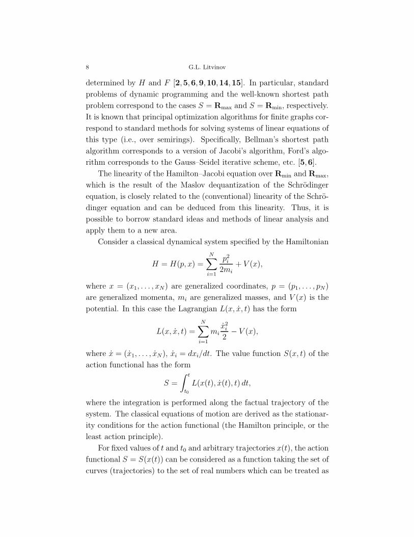
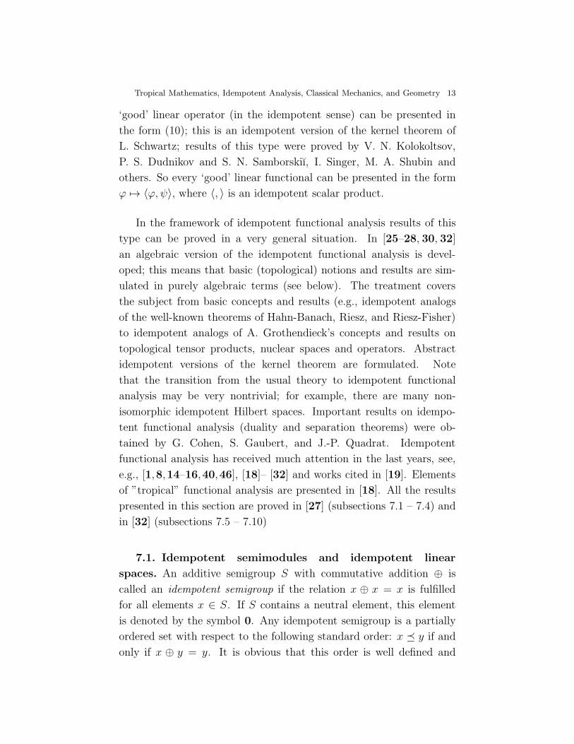
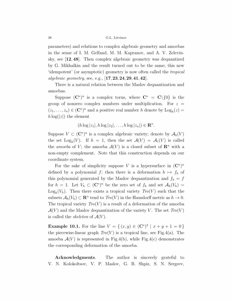
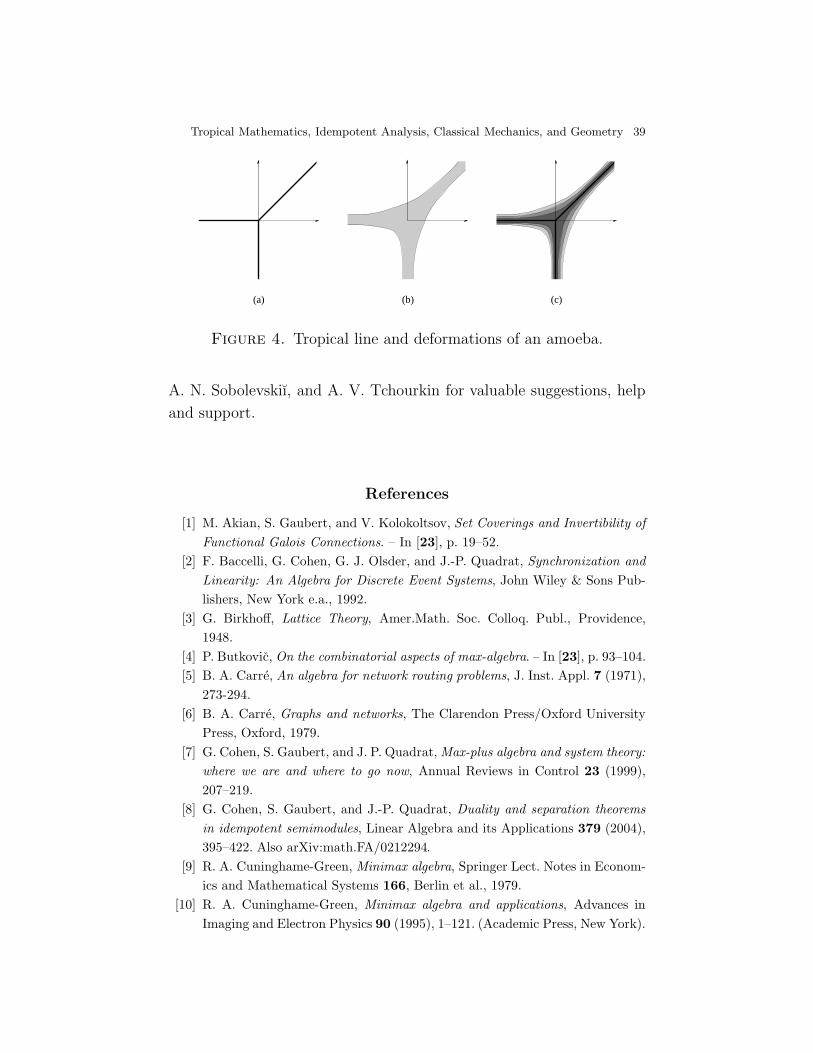
Example 10.1. For the line V = { (x, y) ∈ (C∗)2 | x + y + 1 = 0 }

the piecewise-linear graph Tro(V ) is a tropical line, see Fig.4(a). The

amoeba A(V ) is represented in Fig.4(b), while Fig.4(c) demonstrates

the corresponding deformation of the amoeba.

Acknowledgments. The author is sincerely grateful to

V. N. Kolokoltsov, V. P. Maslov, G. B. Shpiz, S. N. Sergeev,


(a) (c)(b)

Figure 4. Tropical line and deformations of an amoeba.

A. N. Sobolevskiı, and A. V. Tchourkin for valuable suggestions, help

and support.

References

[1] M. Akian, S. Gaubert, and V. Kolokoltsov, Set Coverings and Invertibility of

Functional Galois Connections. – In [23], p. 19–52.

[2] F. Baccelli, G. Cohen, G. J. Olsder, and J.-P. Quadrat, Synchronization and

Linearity: An Algebra for Discrete Event Systems, John Wiley & Sons Pub-

lishers, New York e.a., 1992.

[3] G. Birkhoff, Lattice Theory, Amer.Math. Soc. Colloq. Publ., Providence,

1948.

[4] P. Butkovic, On the combinatorial aspects of max-algebra. – In [23], p. 93–104.

[5] B. A. Carre, An algebra for network routing problems, J. Inst. Appl. 7 (1971),

273-294.

[6] B. A. Carre, Graphs and networks, The Clarendon Press/Oxford University

Press, Oxford, 1979.

[7] G. Cohen, S. Gaubert, and J. P. Quadrat,Max-plus algebra and system theory:

where we are and where to go now, Annual Reviews in Control 23 (1999),

207–219.

[8] G. Cohen, S. Gaubert, and J.-P. Quadrat, Duality and separation theorems

in idempotent semimodules, Linear Algebra and its Applications 379 (2004),

395–422. Also arXiv:math.FA/0212294.

[9] R. A. Cuninghame-Green, Minimax algebra, Springer Lect. Notes in Econom-

ics and Mathematical Systems 166, Berlin et al., 1979.

[10] R. A. Cuninghame-Green, Minimax algebra and applications, Advances in

Imaging and Electron Physics 90 (1995), 1–121. (Academic Press, New York).

http://arxiv.org/abs/math/0212294

40 G.L. Litvinov

[11] P. S. Dudnikov and S. N. Samborskiı, Endomorphisms of semimodules over

semirings with an idempotent operation, preprint of the Mathematical Insti-

tute of the Ukrainian Academy of Sciences, Kiev, 1987 (in Russian).

[12] I. M. Gelfand, M. M. Kapranov, and A. Zelevinsky, Discriminants, resultants,

and multidimensional determinants, Birkhauser, Boston, 1994.

[13] J. S. Golan, Semirings and their applications, Kluwer Acad. Publ., Dordrecht,

1999.

[14] M. Gondran and M. Minoux, Graphes et algorithmes, Editions Eyrolles, Paris,

1979, 1988.

[15] M. Gondran and M. Minoux, Graphes, dioıdes et semi-anneaux, Editions

TEC&DOC, Paris e.a., 2001.

[16] J. Gunawardena (Ed.), Idempotency, Publ. of the Newton Institute, Vol. 11,

Cambridge University Press, Cambridge, 1998.

[17] I. Itenberg, G. Mikhalkin, E. Shustin, Tropical Algebraic Geometry, Oberwol-

fach Seminars, Vol. 35, Birkhauser, Basel e.a., 2007.

[18] V. Kolokoltsov and V. Maslov, Idempotent analysis and applications, Kluwer

Acad. Publ., 1997.

[19] G. L. Litvinov, The Maslov dequantization, idempotent and tropical math-

ematics: a brief introduction, Journal of Mathematical Sciences 140,

#3(2007), 426–444. Also arXiv:math.GM/0507014.

[20] G. L. Litvinov and V. P. Maslov, Correspondence principle for idempotent cal-

culus and some computer applications, (IHES/M/95/33), Institut des Hautes

Etudes Scientifiques, Bures-sur-Yvette, 1995. Also arXiv:math.GM/0101021.

[21] G. L. Litvinov and V. P. Maslov, Idempotent mathematics: correspondence

principle and applications, Russian Mathematical Surveys 51 (1996), no. 6,

1210–1211.

[22] G. L. Litvinov and V. P. Maslov, The correspondence principle for idempotent

calculus and some computer applications. — In [16], p. 420–443.

[23] G. L. Litvinov and V. P. Maslov (Eds.), Idempotent mathematics and mathe-

matical physics, Contemporary Mathematics, Vol. 377, AMS, Providence, RI,

2005.

[24] G. L. Litvinov, V. P. Maslov and S. N. Sergeev (Eds.), International workshop

IDEMPOTENT AND TROPICAL MATHEMATICS AND PROBLEMS OF

MATHEMATICAL PHYSICS, Moscow, Independent Univ. of Moscow, vol.

I and II, 2007. Also arXiv:0710.0377 and arXiv:0709.4119.

[25] G. L. Litvinov, V. P. Maslov, and G. B. Shpiz, Linear functionals on idem-

potent spaces: an algebraic approach, Doklady Mathematics 58 (1998), no. 3,




http://arxiv.org/abs/0710.0377

http://arxiv.org/abs/0709.4119



[26] G. L. Litvinov, V. P. Maslov, and G. B. Shpiz, Tensor products of idempotent

semimodules. An algebraic approach, Mathematical Notes 65 (1999), no. 4,


[27] G. L. Litvinov, V. P. Maslov, and G. B. Shpiz, Idempotent functional analysis.

An algebraic approach, Mathematical Notes 69 (2001), no. 5, 696–729. Also

arXiv:math.FA/0009128.

[28] G. L. Litvinov, V. P. Maslov, and G. B. Shpiz, Idempotent (asymptotic)

analysis and the representation theory. – In: V. A. Malyshev and A. M. Ver-

shik (Eds.), Asymptotic Combinatorics with Applications to Mathematical

Physics. Kluwer Academic Publ., Dordrecht et al, 2002, p. 267–278. Also

arXiv:math.RT/0206025.

[29] G. L. Litvinov, S. N. Sergeev (Eds.), Tropical and Idempotent Mathematics,

Contemporary Mathematics, Vol. 495, AMS, Providence, RI, 2009.

[30] G. L. Litvinov and G. B. Shpiz, Nuclear semimodules and kernel theorems in

idempotent analysis: an algebraic approach, Doklady Mathematics 66 (2002),

no. 2, 197–199. Also arXiv :math.FA/0202026.

[31] G. L. Litvinov and G. B. Shpiz, The dequantization transform and generalized

Newton polytopes. — In [23], p. 181–186.

[32] G. L. Litvinov and G. B. Shpiz, Kernel theorems and nuclearity in idempotent

mathematics. An algebraic approach, Journal of Mathematical Sciences 141,

#4(2007), 1417–1428. Also arXiv:mathFA/0609033.

[33] G. L. Litvinov and G. B. Shpiz, Dequantization procedures related to the

Maslov dequantization. — In [24], vol. I, p. 99–104.

[34] G. G. Magaril-Il’yaev and V. M. Tikhomirov, Convex analysis: theory and

applications, Translations of Mathematical Monographs, vol. 222, American

Math. Soc., Providence, RI, 2003.

[35] Yu. I. Manin, The notion of dimension in geometry and algebra, E-print

arXiv:math.AG/05 02016, 2005.

[36] V. P. Maslov, New superposition principle for optimization problems. — In:

Seminaire sur les Equations aux Derivees Partielles 1985/86, Centre Math.

De l’Ecole Polytechnique, Palaiseau, 1986, expose 24.

[37] V. P. Maslov, On a new superposition principle for optimization problems,

Uspekhi Mat. Nauk, [Russian Math. Surveys], 42, no. 3 (1987), 39–48.

[38] V. P. Maslov, Methodes operatorielles, Mir, Moscow, 1987.

[39] V. P. Maslov, A general notion of topological spaces of negative dimension

and quantization of their densities, Math. Notes, 81, no. 1 (2007), 157–160.

[40] V. P. Maslov and S. N. Samborskii (Eds.), Idempotent Analysis, Adv. Soviet

Math., 13, Amer. Math. Soc., Providence, R.I., 1992.

[41] G. Mikhalkin, Enumerative tropical algebraic geometry in R2, Journal of the

ACM 18 (2005), 313–377. Also arXiv:math.AG/0312530.






42 G.L. Litvinov

[42] G. Mikhalkin, Tropical geometry and its applications, Proceedings of the ICM,

Madrid, Spain, vol. II, 2006, pp. 827–852. Also arXiv:math.AG/0601041v2.

[43] I. V. Roublev, On minimax and idempotent generalized weak solutions to the

Hamilton–Jacobi Equation. – In [23], p. 319–338.

[44] H. H. Schaefer, Topological Vector Spaces, Macmillan, New York a.o., 1966.

[45] I. Simon, Recognizable sets with multiplicities in the tropical semiring. Lecture

Notes in Computer Science 324 (1988), 107–120.

[46] M. A. Shubin, Algebraic remarks on idempotent semirings and the kernel

theorem in spaces of bounded functions. – In: [40], 151–166.

[47] O. Viro, Dequantization of real algebraic geometry on a logarithmic pa-

per. — In: 3rd European Congress of Mathematics, Barcelona, 2000. Also

arXiv:math/0005163.

[48] O. Viro, What is an amoeba?, Notices of the Amer. Math, Soc. 49 (2002),

916–917.

[49] O. Viro, From the sixteenth Hilbert problem to tropical geometry, Japan. J.

Math. 3 (2008), 1–30.

Independent University of Moscow, Bol’shoi Vlasievskii per., 11,

Moscow 119002, Russia

E-mail address : [email protected]



Tropical Mathematics, Idempotent Analysis, Classical Mechanics ...

Documents

Transcript of Tropical Mathematics, Idempotent Analysis, Classical Mechanics ...