Tropical Cyclone Initialization with a Spherical High ...

Tropical Cyclone Initialization with a Spherical High-Order Filter andan Idealized Three-Dimensional Bogus Vortex

IN-HYUK KWON

BK21 Graduate School of Earth Environmental System, Pukyong National University, Busan, South Korea

HYEONG-BIN CHEONG

Department of Environmental Atmospheric Sciences, Pukyong National University, Busan, South Korea

(Manuscript received 13 January 2009, in final form 7 October 2009)

ABSTRACT

A tropical cyclone initialization method with an idealized three-dimensional bogus vortex of an analytic

empirical formula is presented for the track and intensity prediction. The procedure in the new method

consists of four steps: the separation of the disturbance from the analysis, determination of the tropical cy-

clone domain, generation of symmetric bogus vortex, and merging of it with the analysis data. When sepa-

rating the disturbance field, an efficient spherical high-order filter with the double-Fourier series is used whose

cutoff scale can be adjusted with ease to the horizontal scale of the tropical cyclone of interest. The tropical

cyclone domain is determined from the streamfunction field instead of the velocities. The axisymmetric vortex

to replace the poorly resolved tropical cyclone in the analysis is designed in terms of analytic empirical

functions with a careful treatment of the upper-layer flows as well as the secondary circulations. The geo-

potential of the vortex is given in such a way that the negative anomaly in the lower layer is changed into

positive anomaly above the prescribed pressure level, which depends on the intensity of the tropical cyclone.

The geopotential is then used to calculate the tangential wind and temperature using the gradient wind

balance and the hydrostatic balance, respectively. The inflow and outflow in the tropical cyclone are con-

structed to resemble closely the observed or simulated structures under the constraint of mass balance. The

bogus vortex is merged with the disturbance field with the use of matching principle so that it is not affected

except near the boundary of tropical cyclone domain. The humidity of the analysis is modified to be very close

to the saturation in the lower layers near the tropical cyclone center. The balanced bogus vortex of the present

study is completely specified on the basis of four parameters from the Regional Specialized Meteorological

Center (RSMC) report and the additional two parameters, which are derived from the analysis data. The

initialization method was applied to the track and the intensity (in terms of central pressure) prediction of the

TCs observed in the western North Pacific Ocean and East China Sea in 2007 with the use of the Weather

Research and Forecasting (WRF) model. No significant initial jump or abrupt change was seen in either

momentum or surface pressure during the time integration, thus indicating a proper tropical cyclone ini-

tialization. Relative to the results without the tropical cyclone initialization and the forecast results of RSMC

Tokyo, the present method presented a great improvement in both the track and intensity prediction.

1. Introduction

The global analysis for operational use has been im-

proved in both the resolution and accuracy steadily in

recent years, of which the highest horizontal resolution

now available is about 40 km or lower (e.g., Richardson

et al. 2008). It seems, however, that such a high resolu-

tion is still not sufficient to resolve the tropical cyclone

(TC) in detail, particularly in the inner-core region. Even

worse is that the actual resolution of the global analysis is

far lower than the resolution defined by the grid size

because of the coarser resolution of the increments in

the variational data assimilation system (Tremolet 2005;

Grijn et al. 2005). It is not certain whether the accurate

structure of the TC is available even at higher resolution

because of the difficulty of observation. In an attempt to

solve this problem, a sophisticated initialization method

using the bogus vortex has been developed and success-

fully applied to the operational forecast of TCs (Kurihara

et al. 1993, 1995; Bender et al. 2007). The basic idea of

Corresponding author address: Hyeong-Bin Cheong, 599-1

Daeyeon-3-dong, Namgu, Busan 608-737, South Korea.

E-mail: [email protected]

1344 M O N T H L Y W E A T H E R R E V I E W VOLUME 138

DOI: 10.1175/2009MWR2943.1

� 2010 American Meteorological SocietyUnauthenticated | Downloaded 12/25/21 04:36 AM UTC

their initialization method [hereafter referred to as

the Geophysical Fluid Dynamics Laboratory (GFDL’s)

method] is to replace the poorly resolved TC included in

the analysis with a bogus vortex. The bogusing method

has been reported to have contributed to improving the

accuracy of the TC track and intensity prediction (Thu

and Krishnamurti 1992; Serrano and Unden 1994; Leslie

and Holland 1995; Bender et al. 2007).

Recently a new approach to the TC initialization, the

bogus data assimilation (BDA), has emerged, which

uses the four-dimensional variational data assimilation

(4DVAR) technique in combination with the bogus sur-

face pressure (Zou and Xiao 2000; Pu and Braun 2001;

Zhang et al. 2007; Wang et al. 2008). The strategy of BDA

is to suppress the incorporation of the bogus vortex to

a minimum level, and to produce the TC of which vari-

ables are dynamically and physically consistent with one

another. Compared to the cases without TC initialization,

the forecasts were found to be improved with BDA in

both the intensity and structures of the TC. Detailed

structure of the TCs simulated with BDA suggests, how-

ever, that the results would be more improved with a

bogus vortex of a realistic three-dimensional structure.

Common to both bogus method and BDA, the radial

profiles of the surface pressure and tangential wind are

considered as the most fundamental factors needed in

deriving the initial TC structure of the prediction model.

They are usually given as the analytic empirical function

(e.g., Fujita 1952; Holland 1980; Chan and Williams

1987). The empirical formulas are not only found to be

well supported by the observation but also proved useful

in studying the dynamics associated with the TC. Con-

sidering that the upper structures of the TC are strongly

tied up with the surface pressure (or wind), the infor-

mation on the surface structure may be used in estima-

ting the upper structures to a good approximation. Such

a strategy was adopted in the simulations of the TCs

(Iwasaki et al. 1987; Mathur 1991; Kurihara et al. 1993,

1995). Iwasaki et al. (1987) attempted to specify the ver-

tical variation of geopotential perturbation in terms of

empirical function. The detailed structure of the model

typhoon, however, was not consistent with the observa-

tion. For example, the anticyclonic flow was set as strong

as the cyclonic flow and was given to extend down to the

tropospheric midlevel. Mathur (1991) introduced an an-

alytic empirical function for the wind structure from the

surface to the upper levels. The wind strength was given

to decrease upward and the wind direction changes from

the cyclonic flow to the anticyclonic in the upper layers.

In GFDL’s method the target tangential wind of the

axisymmetric model is prescribed based on the obser-

vation in such a way that its magnitude is monotonically

reduced upward. The perturbation was not specified above

150 hPa. As long as the qualitative structure of the ob-

served TC rather than the detailed structure is thought

to be important as the initial condition, it would be

possible to introduce an analytic empirical function to

the vertical dependency of the pressure or tangential

wind deviation in the TC. Similarly, the radial-vertical

circulation may also be specified explicitly by empirical

formula without resorting to the time integration of the

axisymmetric model or assimilation model.

The asymmetric component, often called as the beta

gyre, is known to play an important role in moving the

vortex itself (Holland 1983; Carr and Elsberry 1992;

Smith 1993; Williams and Chan 1994; Kurihara et al.

1993, 1995). The asymmetric component in the bogusing

method for TC initialization is usually generated by

running a simplified model (e.g., Kurihara et al. 1993,

1995). The beta gyre includes a wide range of horizontal

scales from the smaller scales than the symmetric com-

ponent to larger scales. Among them the larger-scale

component of the beta gyre is believed to constitute

a steering current for the vortex while the smaller scale is

relatively of minor importance. Therefore, if there is

a possibility that the larger-scale part of the beta gyre

remains in the basic field at the time of separation of the

disturbance from the analysis, the bogus vortex may be

constructed without considering the asymmetric com-

ponent. In that case the filter that can give a rather sharp

cutoff may be required.

In this study, a bogusing method is presented for the

TC track and intensity prediction, which incorporates

the spherical high-order filter with double-Fourier series

capable of giving sharp cutoff and the empirical for-

mulas for the variables in the axisymmetric components.

In the following section, the detailed procedure to con-

struct bogus vortex is presented. In section 3, the quality

of the bogus vortex is checked in terms of vertical sigma

velocity. Section 4 presents the case studies on the track

and the intensity prediction with the new bogus method

for the TCs observed in the western North Pacific and

East China Sea in 2007. Discussion and conclusions are

given in the final section.

2. TC initialization method with the three-dimensional bogus vortex

a. Overview of the new initialization method

The new method of TC initialization for the track and

intensity prediction is outlined in Fig. 1. It consists of

four steps: 1) input of Regional Specialized Meteoro-

logical Center (RSMC) TC information and splitting of

the global analysis data into basic field and disturbance,

2) determination of TC domain in the disturbance field,

3) design of idealized three-dimensional axisymmetric

APRIL 2010 K W O N A N D C H E O N G 1345

Unauthenticated | Downloaded 12/25/21 04:36 AM UTC

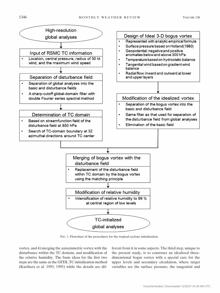
vortex, and 4) merging the axisymmetric vortex with the

disturbance within the TC domain, and modification of

the relative humidity. The basic ideas for the first two

steps are the same as the GFDL TC initialization method

(Kurihara et al. 1993, 1995) while the details are dif-

ferent from it in some aspects. The third step, unique to

the present study, is to construct an idealized three-

dimensional bogus vortex with a special care for the

upper levels and secondary circulation, where target

variables are the surface pressure, the tangential and

FIG. 1. Flowchart of the procedures for the tropical cyclone initialization.



radial wind, and the geopotential perturbation and

corresponding temperature perturbation in hydrostatic

balance. In the final step, the axisymmetric vortex is

merged into the disturbance of the analysis within the TC

domain using a matching principle to make a smoothly

varying field over the region near the boundary. After

this, the relative humidity of the global analyses is mod-

ified to facilitate rapid condensation at the central region

in the lower layers.

b. Global-domain filtering of the global analyses

Tropical cyclone initialization in the present study

begins with splitting of the global analysis into the basic

field and disturbance as is done in the GFDL method

(Kurihara et al. 1993, 1995). In the GFDL method, the

scale separation is done by filtering the horizontal two-

dimensional grid point data with a digital filter (or smooth-

ing operator; also known as Kurihara filter), which con-

sists of a three-point spatial operator (Kurihara et al.

1993, 1995). Kurihara’s filter is one-dimensional spatial

operator, which is applied to the zonal direction first and

then to the meridional direction subsequently.

In this study a high-order double-Fourier series (DFS)

spectral filter, instead of the grid point operator, is used

to separate the basic field and the disturbance from

global analysis (Cheong et al. 2002, 2004). It performs

filtering with the O(N2 log2N) operation count for the

data of O(N2) grid points by inverting the tridiagonal

matrices whose elements are the spectral components in

the DFS expansion of a variable on the sphere. The

tridiagonal matrices are constructed based on the high-

order Helmholtz equation:

[1 1 n(�1)q=2q]z* 5 z, (1)

where z* (z) is the filtered (to be filtered) variable de-

fined on a spherical surface, n denotes the filter co-

efficient, q is the filter order (being positive), and =2 [

(1/a2cos2u)[(›2/›l2) 1 cosu(›/›u)cosu(›/›u)] with a, l,

and u being the earth’s radius, the longitude, and the

latitude, respectively.

The spectral filter is isotropic on the spherical surface

as it gives the same damping rate for the disturbances of

a certain horizontal scale regardless of their meridional

locations. As the filter order increases, a sharper split-

ting of the global analysis is achieved. The response

function of the spectral filter Rl is given by

Rl5

1

[1 1 n(a2cl)q]

, (2)

where cl 5 l(l 1 1) with l being the degree of the Legendre

function [i.e., the total wavenumber-like index on the

spherical surface (l is referred to as spherical wave-

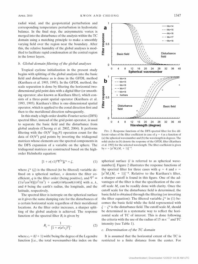
number)]. Figure 2 illustrates the response functions of

the spectral filter for three cases with q 5 4 and v 5

[a2Mc(Mc 1 1)]2q. Relative to the Kurihara’s filter,

a sharper cutoff is found in this figure. One of the ad-

vantages of the filter is that the specification of the cut-

off scale Mc can be readily done with clarity. Once the

cutoff scale for the disturbance field is determined, the

basic field is obtained through the filtering (or inverting

the filter equation): The filtered variable z* in (1) be-

comes the basic field while the field represented with

z 2 z* is the disturbance field. The cutoff scale Mc should

be determined in a systematic way to reflect the hori-

zontal scale of TC of interest. This is done following

the criteria with the use of the radius of 15 m s21 and TC

intensity (see Table 1).

c. Determination of the TC domain

It is assumed that the horizontal extent of the TC is

restricted to a finite distance from the center. For

FIG. 2. Response functions of the DFS spectral filter for five dif-

ferent values of the filter coefficient in case of q 5 4 as a function of

(a) the spherical wavenumber and (b) the wavelength in degrees. The

solid circles in (b) denote the response of the GFDL filter (Kurihara

et al. 1993) for the selected wavelength. The filter coefficient is given

by v 5 [a2Mc(Mc 1 1)]24.



convenience, this finite domain is referred to as the TC

domain. The TC domain is very similar to the filter do-

main defined in the GFDL method, but not exactly the

same. As is done in the GFDL method, the TC domain

should be determined large enough to contain the bogus

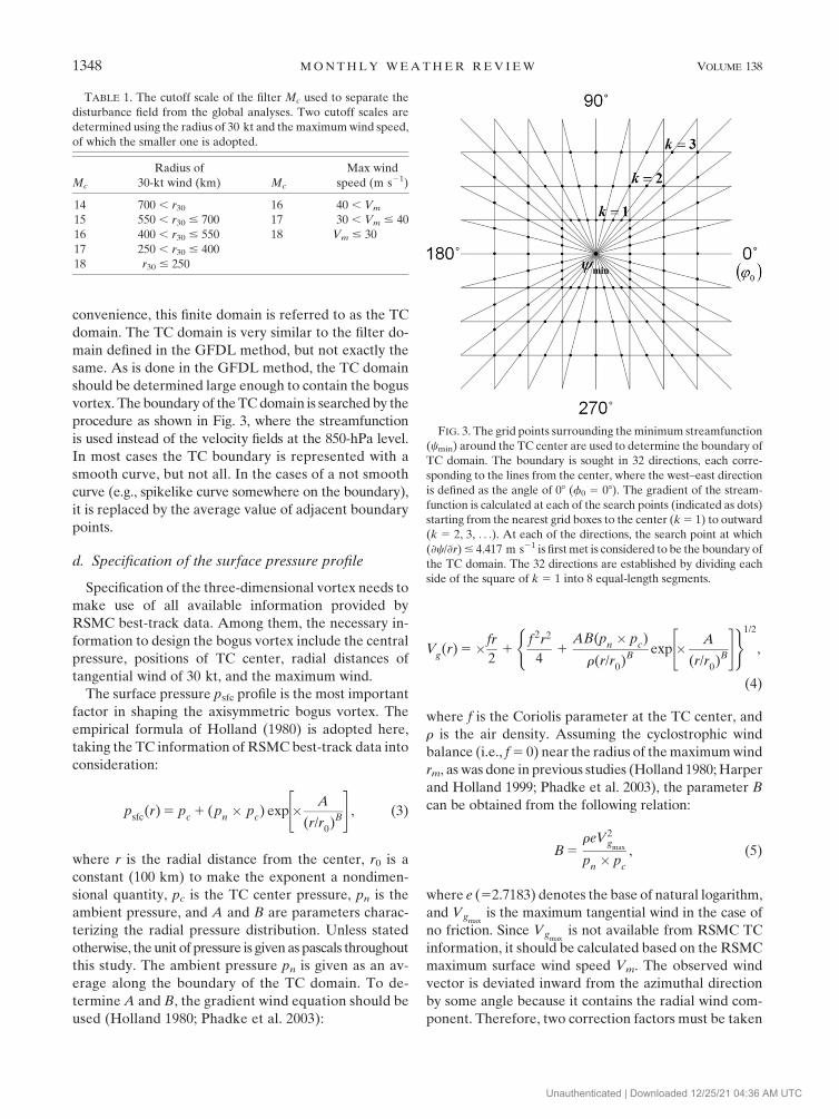
vortex. The boundary of the TC domain is searched by the

procedure as shown in Fig. 3, where the streamfunction

is used instead of the velocity fields at the 850-hPa level.

In most cases the TC boundary is represented with a

smooth curve, but not all. In the cases of a not smooth

curve (e.g., spikelike curve somewhere on the boundary),

it is replaced by the average value of adjacent boundary

points.

d. Specification of the surface pressure profile

Specification of the three-dimensional vortex needs to

make use of all available information provided by

RSMC best-track data. Among them, the necessary in-

formation to design the bogus vortex include the central

pressure, positions of TC center, radial distances of

tangential wind of 30 kt, and the maximum wind.

The surface pressure psfc profile is the most important

factor in shaping the axisymmetric bogus vortex. The

empirical formula of Holland (1980) is adopted here,

taking the TC information of RSMC best-track data into

consideration:

psfc

(r) 5 pc1 (p

n� p

c) exp� A

(r/r0)B

" #, (3)

where r is the radial distance from the center, r0 is a

constant (100 km) to make the exponent a nondimen-

sional quantity, pc is the TC center pressure, pn is the

ambient pressure, and A and B are parameters charac-

terizing the radial pressure distribution. Unless stated

otherwise, the unit of pressure is given as pascals throughout

this study. The ambient pressure pn is given as an av-

erage along the boundary of the TC domain. To de-

termine A and B, the gradient wind equation should be

used (Holland 1980; Phadke et al. 2003):

Vg(r) 5�fr

21

f 2r2

41

AB(pn� p

c)

r(r/r0)B

exp � A

(r/r0)B

" #( )1/2

,

(4)

where f is the Coriolis parameter at the TC center, and

r is the air density. Assuming the cyclostrophic wind

balance (i.e., f 5 0) near the radius of the maximum wind

rm, as was done in previous studies (Holland 1980; Harper

and Holland 1999; Phadke et al. 2003), the parameter B

can be obtained from the following relation:

B 5reV2

gmax

pn� p

c

, (5)

where e (52.7183) denotes the base of natural logarithm,

and Vgmaxis the maximum tangential wind in the case of

no friction. Since Vgmaxis not available from RSMC TC

information, it should be calculated based on the RSMC

maximum surface wind speed Vm. The observed wind

vector is deviated inward from the azimuthal direction

by some angle because it contains the radial wind com-

ponent. Therefore, two correction factors must be taken

FIG. 3. The grid points surrounding the minimum streamfunction

(cmin) around the TC center are used to determine the boundary of

TC domain. The boundary is sought in 32 directions, each corre-

sponding to the lines from the center, where the west–east direction

is defined as the angle of 08 (f0 5 08). The gradient of the stream-

function is calculated at each of the search points (indicated as dots)

starting from the nearest grid boxes to the center (k 5 1) to outward

(k 5 2, 3, . . .). At each of the directions, the search point at which

(›c/›r) # 4.417 m s21 is first met is considered to be the boundary of

the TC domain. The 32 directions are established by dividing each

side of the square of k 5 1 into 8 equal-length segments.

TABLE 1. The cutoff scale of the filter Mc used to separate the

disturbance field from the global analyses. Two cutoff scales are

determined using the radius of 30 kt and the maximum wind speed,

of which the smaller one is adopted.

Mc

Radius of

30-kt wind (km) Mc

Max wind

speed (m s21)

14 700 , r30 16 40 , Vm

15 550 , r30 # 700 17 30 , Vm # 40

16 400 , r30 # 550 18 Vm # 30

17 250 , r30 # 400

18 r30 # 250



into consideration to estimate Vgmax

. One is the frictional

effect, and the other is the inflow angle:

Vgmax

5V

m

K0

cosb0, (6)

where K0 is the correction factor due to friction, given as

0.8 (Harper and Holland 1999; Phadke et al. 2003), and

b0 means the inflow angle, specified as 208 at rm (Phadke

et al. 2003). The inflow angle varies with the radial dis-

tance, which will be discussed in more detail later at the

time of specifying the radial flow. Because of these two

correction factors, the wind speed in the RSMC best-

track data should be changed in a similar way to (6). For

example, as for the 30-kt wind information, the wind

speed may be modified to give Vg30

[[(30 kt/K0) cosb

1] ’

34 kt with b1 5 258, where the radius of 30 kt was as-

sumed to be much larger than rm so that the inflow angle

is determined as 258 (Phadke et al. 2003).

If the information from RSMC on the radial distance of

30-kt wind speed is used in (4) with the corrected value as

shown above, A is calculated using an iteration method

(Kwon 2002): for this purpose, the function that will be

used in the iteration is defined by incorporating the radius

of 30 kt (r30) and the modified gradient wind at r30 (Vg30

):

W(A) 5�Vg30�

fr30

2

1f 2r2

30

41

AB(pn� p

c)

r(r30

/r0)B

exp � A

(r30

/r0)B

" #( )1/2

.

(7)

Then, by the Newton–Raphson’s iteration method (Press

et al. 1992), the parameter A can be obtained:

Ai11

5 Ai�W(A)

dW

dA

� ��1

, (8)

where i means the step of iteration. Starting from a

proper initial guess for A (set close to zero) and a pre-

determined threshold value for convergence, it was

possible to find the solution with several steps. In the

case where the solution is not converged during itera-

tion, the RSMC information on r30 is slightly modified

for numerical reasons.

With the parameters A and B, the surface pressure psfc

can be determined completely as a function of the radial

distance. From (4) rm is obtained from rm 5 r0A1/B. In

the case where rm . 100 km or rm , 40 km, it is adjusted

to be 100 or 40 km, respectively. Then the parameter A

is recalculated from A 5 (rm/r0)B, which should be used

to determine the surface pressure psfc.

e. Design of three-dimensional vortex

In this subsection, an axisymmetric bogus vortex of

three dimensions will be designed empirically in terms of

analytic functions taking into consideration the important

features of observed and simulated tropical cyclones.

Since the bogus vortex is used to replace the typhoon in

the disturbance field, it consists of only the deviation from

the large-scale basic field. The characteristics of the bogus

vortex that is to be built hereafter are as follows:

d Horizontal structures of the geopotential, tangential

and radial wind, and temperature field in the 3D bogus

FIG. 4. A schematic diagram illustrating the structure of (left) geopotential deviation (F9b) in

the ideal bogus vortex, where psfc, pc, and pn denote the surface pressure, central pressure, and

ambient pressure, respectively. The geopotential deviation has the negative maximum value

over the center at the surface level, whose magnitude decreases upward and in the radial di-

rection. The positive anomaly maximum is given at pa and the vertical extent of the positive

anomaly increases as the (right) radial distance becomes large.



vortex are determined primarily by the surface pres-

sure profile.d Tangential wind and temperature are tied up with one

variable, the geopotential, in terms of the gradient

wind balance in horizontal plane and the hydrostatic

equilibrium in the vertical, respectively.d The maximum tangential wind is found at the radial

distance of the approximate largest gradient of surface

pressure.d The maximum temperature anomaly exists in the up-

per troposphere.d The geopotential in the central region has the largest

negative value at the surface and increases with height

monotonically, which then changes its sign to positive

near tropopause. The pressure level of the positive

maximum is kept constant, whereas the vertical extent

of the positive anomaly broadens downward as the

radial distance increases, as shown schematically in

Fig. 4.d The secondary circulation that maintains the mass

balance has the strongest upward motion in the mid-

tropospheric level at the radius of maximum tangen-

tial wind, and maintains inflow and outflow in the

lower and upper layers, respectively.d In the outflow layers, the tangential wind is cyclonic

rotation near the center, but anticyclonic rotation off

the central region; the vertical extent of the anticy-

clonic rotation broadens downward as the radial dis-

tance increases.

The first variable to be constructed for the 3D bogus

vortex is geopotential because it will be used to deter-

mine other variables. The average structure of the axi-

symmetric geopotential field of TC is well represented

with a negative anomaly and a positive anomaly in the

lower and upper level, respectively, as indicated by

many observational and numerical studies (Frank 1977;

Iwasaki et al. 1987; Liu et al. 1999; Braun et al. 2006).

The strategy for specifying the axisymmetric geo-

potential field resembling the observed structure as

much as possible is as follows: two radial functions are

defined at the level of maximum positive anomaly (pa)

and the surface (psfc), respectively. To take the intensity

of the TC into consideration, pa is given to vary with pc

of the TC (see Table 2). Next, the radial functions are

combined together with a function that gives the vertical

distribution. The upper-level function was designed in

such a way that the cyclonic rotation is maintained near

the center of the upper levels. The geopotential deviation

(defined as the difference from the environment) at pa, is

given as

F9u(r) 5 x(u

c)

pn� p

c

103 hPa

� �1� tanh

r � ra

0.4ra

� ��

3 exp � A

(r/r0)B

" #(9a)

x(uc) 5 7 3 103 tanh2 u

c

u0

� �, (9b)

where uc is the latitude of TC center, u0 5 308, and ra

(5 r30 1 700 km) is the radius of maximum anticyclonic

rotation. The function in the first bracket of (9a), which

is associated with the anticyclonic rotation in the outer

region, and the factor of the exponential function were

chosen deliberately to give an almost-zero anomaly at

the center. Adoption of the function in the square bracket

was found to give a broad anticyclonic jet like structure in

the upper layers, as resembles the observed structure

(e.g., Frank 1977). The function x(uc) was introduced to

avoid breakdown of the gradient wind balance because of

a too large negative value of the geopotential gradient.

The constant parameters that appear in (9) and will ap-

pear in other equations below are produced empirically

based on the trial and error to best fit the observed or

simulated tropical cyclones. The geopotential deviation

at the surface is assumed to be proportional to the pres-

sure deviation, as was done in Mathur (1991). To the

formula used by Mathur (1991), an additional term is

introduced to account for dependency of air density to

the pressure. Then, the geopotential deviation at the

surface level is given as

F9b(r) 5�

RT0

psfc

(pn� p

sfc), (10)

where T0 is the surface temperature averaged in the

inner region of the TC domain (r # 100 km) and R

represents the gas constant. The pressure dependent

term in (10) allows the surface geopotential to closely

follow the surface pressure structure.

The geopotential deviation above pa is produced by

introducing a simple function to the formula in (9). On the

other hand, the geopotential deviation between pa and the

surface is constructed by coupling two functions defined at

pa and psfc in terms of a sophisticated vertical function.

With carefully chosen vertical functions, the radial-vertical

function for the geopotential deviation is written as

TABLE 2. The pressure level of the maximum positive geopotential

anomaly ( pa) as a function of the central pressure ( pc).

pa (hPa) Central pressure range (hPa)

120 pc , 945

130 945 # pc , 960

140 960 # pc , 980

150 980 # pc



F9(r, p) 5F9

uexp �3

pa

p� 1

� �2" #

for p # pa

(11a)

F9u

1 (F9b�F9

u)(E 1 sm) for p $ p

a(11b)

8><>:

E 5sech(tj)� 1

sech(t)� 1, (11c)

m 5 j2(j � 1)(�3j 1 4), (11d)

where j 5 (p 2 pa)(psfc 2 pa)21, t is a parameter that

controls the vertical structure, and the function s [[s(r)]

is used to match the surface boundary condition in re-

lation with the hydrostatic temperature. From the na-

ture of the vertical function in (11b), the larger value of t

results in sharper variation of geopotential. Through

a series of sensitivity tests, the effect of the parameter t

was found to be more important for the temperature

anomaly than the geopotential. Therefore, how to de-

termine the parameter t will be stated later in relation

with the temperature anomaly. It is obvious that the

geopotential at pa (j 5 0) and surface (j 5 1) turns out to

be identical to F9u and F9b, respectively.

The temperature deviation for the axisymmetric

vortex is derived from the geopotential field using the

hydrostatic balance equation. Since the bogus vortex

under consideration is an approximate model of the

TC, this assumption is not likely to be inappropriate

for this problem. The temperature deviation is, then,

given as

T9(r, p) [�p

R

›F9

›p(12a)

5

�6

R

paF9

u

p

pa

p� 1

� �exp �3

pa

p� 1

� �2" #

for p # pa

(12b)

�p

R

F9b�F9

u

psfc� p

a

[F � sj(12j2 � 21j 1 8)] for p $ pa, (12c)

8>>>><>>>>:

where

F [ F(j) 5 (psfc� p

a)

dE

dp

5�tsech(tj) tanh(tj)

sech(t)� 1. (13)

Substitution of the boundary condition T9(r, psfc) 5

Tb*(r) into (12c) yields the following equation for s as a

function of radius:

s(r) 5� F(1) 1T

b*R

psfc

psfc� p

a

F9b�F9

u

� �, (14)

with Tb*(r) being defined as the surface temperature devia-

tion at radius r from the ambient [i.e., Tsfc(r) 2 Tr52000 km]

on the isobaric surface. If the assumption is made that

the temperature difference vanishes at the surface level,

Tb*(r) can be obtained by the following equation:

Tb*(r) 5� G

g0

F9b

5GRT

0

g0

psfc

(pn� p

sfc), (15)

where G is temperature lapse rate specified as 0.008 K m21.

Therefore, the constant T0 acts like a hinge variable that

makes the bogus vortex rest on the observed surface

condition. The parameter t characterizes the vertical

structure of geopotential deviation as mentioned above,

and hence it also affects the vertical structure of the

temperature deviation, particularly the height of the

warm core. A sensitivity test for the parameter t indi-

cates that the temperature anomaly slightly exceeding

10 K appears around the 300-hPa level for the moderate

size of the tropical cyclone. These features were found to

be realized with t 5 5 ; 6, of which t 5 5.5 was used in

this study.



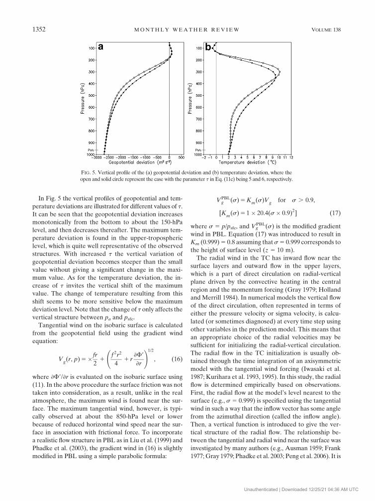
In Fig. 5 the vertical profiles of geopotential and tem-

perature deviations are illustrated for different values of t.

It can be seen that the geopotential deviation increases

monotonically from the bottom to about the 150-hPa

level, and then decreases thereafter. The maximum tem-

perature deviation is found in the upper-tropospheric

level, which is quite well representative of the observed

structures. With increased t the vertical variation of

geopotential deviation becomes steeper than the small

value without giving a significant change in the maxi-

mum value. As for the temperature deviation, the in-

crease of t invites the vertical shift of the maximum

value. The change of temperature resulting from this

shift seems to be more sensitive below the maximum

deviation level. Note that the change of t only affects the

vertical structure between pa and psfc.

Tangential wind on the isobaric surface is calculated

from the geopotential field using the gradient wind

equation:

Vg(r, p) 5�fr

21

f 2r2

41 r

›F9

›r

!1/2

, (16)

where ›F9/›r is evaluated on the isobaric surface using

(11). In the above procedure the surface friction was not

taken into consideration, as a result, unlike in the real

atmosphere, the maximum wind is found near the sur-

face. The maximum tangential wind, however, is typi-

cally observed at about the 850-hPa level or lower

because of reduced horizontal wind speed near the sur-

face in association with frictional force. To incorporate

a realistic flow structure in PBL as in Liu et al. (1999) and

Phadke et al. (2003), the gradient wind in (16) is slightly

modified in PBL using a simple parabolic formula:

VPBLg (s) 5 K

m(s)V

gfor s . 0.9,

[Km

(s) 5 1� 20.4(s � 0.9)2] (17)

where s 5 p/psfc, and VgPBL(s) is the modified gradient

wind in PBL. Equation (17) was introduced to result in

Km (0.999) 5 0.8 assuming that s 5 0.999 corresponds to

the height of surface level (z 5 10 m).

The radial wind in the TC has inward flow near the

surface layers and outward flow in the upper layers,

which is a part of direct circulation on radial-vertical

plane driven by the convective heating in the central

region and the momentum forcing (Gray 1979; Holland

and Merrill 1984). In numerical models the vertical flow

of the direct circulation, often represented in terms of

either the pressure velocity or sigma velocity, is calcu-

lated (or sometimes diagnosed) at every time step using

other variables in the prediction model. This means that

an appropriate choice of the radial velocities may be

sufficient for initializing the radial-vertical circulation.

The radial flow in the TC initialization is usually ob-

tained through the time integration of an axisymmetric

model with the tangential wind forcing (Iwasaki et al.

1987; Kurihara et al. 1993, 1995). In this study, the radial

flow is determined empirically based on observations.

First, the radial flow at the model’s level nearest to the

surface (e.g., s 5 0.999) is specified using the tangential

wind in such a way that the inflow vector has some angle

from the azimuthal direction (called the inflow angle).

Then, a vertical function is introduced to give the ver-

tical structure of the radial flow. The relationship be-

tween the tangential and radial wind near the surface was

investigated by many authors (e.g., Ausman 1959; Frank

1977; Gray 1979; Phadke et al. 2003; Peng et al. 2006). It is

FIG. 5. Vertical profile of the (a) geopotential deviation and (b) temperature deviation, where the

open and solid circle represent the case with the parameter t in Eq. (11c) being 5 and 6, respectively.



known to vary with the height and radial distance to a

large extent. Unfortunately, no universal formula for the

inflow angle is found in the literature. To specify the

inflow angle for the bogus vortex, the empirical formula

of Phadke et al. (2003) is adopted with a minor modifi-

cation: a continuous variation of the inflow angle b is

chosen rather than piecewise variations over subdivided

radial intervals:

b 550(r/r

m)4 � 12.5

4(r/rm

)41 1

1 12.5, (18)

which gives b(rm) 5 208, being identical to the value

used for the correction of the maximum surface wind.

The radial variation of the inflow angle is presented in

Fig. 6 along with the empirical formula proposed by

Phadke et al. (2003). The inflow angle of the new scheme

varies from 258 at r . rm to 08 at r 5 0, while the formula

of Phadke et al. (2003) maintains some angle even near

the center. In the region rm # r # 1.2rm, rather steep

variations for both curves can be seen. Use of the con-

tinuous function for the inflow angle was found to con-

tribute to establishing a smooth field of vertical sigma

velocity diagnosed with radial velocity, as will be shown

below. The radial velocity at the surface level (s 5

0.999) is then calculated with the use of the tangential

wind and the inflow angle:

vr* 5�(VPBL

g )s50.999

tanb, (19)

where vr* and (VgPBL)s50.999 are the radial and tangential

winds at the surface level, respectively.

On formulating the radial wind in empirical way, it is

assumed that the inflow occurs mostly in the lower levels

with the strongest inflow near the surface (s 5 0.98).

The radial inflow should be given in such a way that the

inflow angle should decrease with height. The outflow is

determined to keep its maximum strength near the level

of maximum geopotential deviation (pa). One impor-

tant issue in this procedure is to maintain the mass bal-

ance between the inflow and outflow regions in order to

facilitate the rapid adjustment of the bogus vortex to the

prediction model. Considering this point, the empirical

function for radial wind is specified as

vr(r, s) 5

q1

sech[45(s � sa)] for s , s

a

q1

sech[c(s � sa)] 1 q

0sech[d(s � 0.98)] for s

a# s , 0.98

q0

sech[15(s � 0.98)] for 0.98 # s

8><>: , (20)

where sa is defined as pa/psfc, c [[c(r)], and d [[d(r)] are

nondimensional factors to shape the radial wind, and q0 and

q1 are functions of radius. The factors c and d are given by

c(r) 5 8 1 37 tanhr

167 km

� �exp � r

350 km� 1

� �2� �

(21a)

d(r) 5 7 1p

a

5 hPa� 0.5c. (21b)

With the use of the boundary condition at the surface, q0

is obtained as

q0

5v

r*

sech[15(0.999� 0.98)]. (22)

The factor q1 is determined from the requirement that

net mass flux through the cylindrical surface from bot-

tom to the model top sT should vanish:

ð0.98

sa

q0

sech[d(s � 0.98)] ds 1

ð1

0.98

q0

sech[15(s � 0.98)] ds 1

ð0.98

sa

q1

sech[c(s � sa)] ds

1

ðsa

sT

q1

sech[45(s � sa)] ds 5 0, (23)

FIG. 6. Radial distributions of the inflow angle used in this study

(open circle) and in Phadke et al. (2003; solid circle), respectively.



which yields

q1

5�q0

1

darctaned(s�0.98)

��1

0.98

11

15arctane15(s�0.98)

��1

0.98

1

carctanec(s�s

a)

��0.98

sa

11

45arctane45(s�s

a)

��s

a

sT

.

(24)

The top level sT is specified small enough to be far above

the level of maximum geopotential deviation: sT 5 0.01.

f. Merging the axisymmetric vortex with thedisturbance

Before merging with the disturbance field, the axi-

symmetric bogus vortex should be filtered in order to

eliminate the large-scale component. The order and

coefficient of the filter are the same as used in section 2b.

The filtered axisymmetric vortex is merged with the dis-

turbance field within the TC domain keeping the distur-

bance field unaffected outside the TC domain. Since in

the second step the TC domain was set large enough to

include the axisymmetric component in it, there should

remain a transition zone from the vortex periphery to the

TC boundary. For the GFDL method this transition zone

is occupied by the hurricane component within the TC

domain. In the present method, however, the nonhur-

ricane component is not separated from the disturbance

field within the TC domain. It is certain that a simple

replacement of the disturbance by the axisymmetric

vortex will result in the discontinuity at the periphery of

the vortex. As a cure for this problem a matching function

is introduced to give a smooth transition from the bogus

vortex to the disturbance with the TC domain. This

function is designed in a similar manner in Mathur (1991)

to affect little the bogus vortex as well as the disturbance

near the TC boundary. With the function the merged field

is represented with the following equation:

Sc5 W

m(G

d� S

i) 1 S

i, (25)

where Sc means the merged field, Wm denotes the

matching function, Gd and Si represent the disturbance

field within TC domain and the axisymmetric vortex,

respectively. The matching function is given as

Wm

5 e�[(r�rd)/0.3r

d]2, (26)

where r and rd are the distance of the grid point from the

storm center and the radial distance to the TC boundary,

respectively.

g. Modification of the humidity field near the stormcenter

An idealized structure for the humidity is not consid-

ered in the axisymmetric vortex. Instead, the humidity of

the global analysis is modified in the lower central region

of the storm based on the fact that the global analysis

often fails to provide the accurate moisture field: in some

cases the relative humidity in that region is analyzed to be

far from being saturation, which may cause the incorrect

or delayed development of the tropical cyclone in the

numerical model. The moisture field is, then, modified by

RH 5 RHa

1 (RHb�RH

a)

3 exp �8 lnp

p0

� �2

� 10

lnr

h1 hr

rh

1 hrm

� �ln(1 1 0.556h)

2664

3775

28>>><>>>:

9>>>=>>>;

,

(27)

where p0 5 1000 hPa, h 5 (r30/rm)2, rh 5 900 Km, RH,

and RHa are the modified and analyzed relative hu-

midity, respectively; RHb is a constant value of 99%.

3. Quality check of the empirical bogus vortex

Shown in Fig. 7 are the radial-vertical distributions of

the geopotential deviation, the temperature deviation,

the tangential wind, and the radial wind of the idealized

bogus vortex relevant to Typhoon Nari (11 September

2007), which is one of the TCs simulated in this study

(see Table 3). Typhoon Nari is characterized as a small-

sized but intense tropical cyclone, exhibiting the in-

tensity of about 935 hPa with a maximum wind speed

exceeding 100 m s21 at 1200 UTC 14 September 2007.

A strong vortexlike structure is well represented with the

geopotential deviation and the tangential wind, of which

maximum values are found in the surface and at the

900-hPa level, respectively. Geopotential deviation shows

weak positive anomaly in the upper layers whose verti-

cal extent is broadened with the radius, as is the case of

the observed structure. The temperature deviation ex-

hibits the maximum value around the 300-hPa level and

negative values above about the 150-hPa level, quite

similar to the well-developed tropical cyclones (Frank

1977). Except for the inner-core region the radial flow

increases as the radial distance decreases, common to

both the lower and upper layers. The maximum gradient

of radial wind is found over r ’ rm. All these features are

quite reminiscent of the essential features of observed or

simulated tropical cyclones in a qualitative sense (Frank

1977; Anthes 1982; Liu et al. 1999).



Whether the empirical bogus vortex is specified ap-

propriately or not can be checked by calculating the

vertical sigma velocity based on the continuity equation.

The surface pressure equation (i.e., the mass conserva-

tion equation), in the cylindrical coordinate system with

the vertical sigma coordinate is written as

› ln ps

›t1 v

r

› ln ps

›r1 D 1

› _s

›s5 0, (28)

where D [[(1/r)(›/›r)rvr] represents the horizontal di-

vergence on a constant sigma level. Integration of (28)

from s 5 0 to s 5 1 results in › ln ps/›t 5 0 because of the

conditionsÐ 1

0 vr

ds 5 0 and _s(0) 5 _s(1) 5 0. There-

fore, the vertical sigma velocity can be written as

_s 5

ð1

s

vr

› ln ps

›r1

1

r

›

›rrv

r

� �ds. (29)

The vertical sigma velocity on the radial-vertical plane is

presented in Fig. 8, which is associated with the bogus

fields in Fig. 7. A well-organized vertical velocity is

clearly seen near the storm center, as can be observed

for developed TC. The maximum absolute value,

slightly larger than 9 3 1025 s21, occurs at about r 5 rm,

and decreases away from there.

It may be emphasized that the two variables, the

surface pressure and radial velocity, which appear in the

sigma velocity in Eq. (29), were made systematically

dependent on other variables defining the bogus vortex

in direct or indirect ways. For example, the empirical

function for the radial velocity is constructed in terms of

the tangential wind that is associated with the geo-

potential, which is originally built upon the surface

pressure function. Therefore, it seems quite reasonable

to judge the adequacy of the bogus vortex in terms of the

vertical sigma velocity upon the internal consistency

among variables.

As mentioned in the previous section, the bogusing

method in this study generates a bogus vortex whose

structure and size can be determined on the basis of the

RSMC TC information. To illustrate the high adapt-

ability of the bogusing method to the RSMC TC in-

formation, the bogus vortices of four cases selected from

FIG. 7. Radial-vertical cross sections of the empirical bogus vortex for the variables of (a) the geopotential de-

viation (m2 s22), (b) the temperature deviation (K), (c) the tangential wind (m s21), and (d) the radial wind (m s21).

The curve at the bottom in each map represents the surface pressure. The bogus vortex was specified to initialize

Typhoon Nari at 0000 UTC 14 Sep 2007.



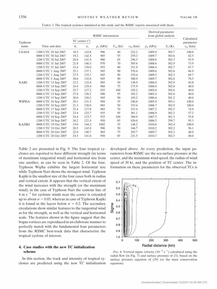
Table 2 are presented in Fig. 9. The four tropical cy-

clones are reported to have different strength (in terms

of maximum tangential wind) and horizontal size from

one another, as can be seen in Table 2. Of the four,

Typhoon Wipha exhibits the largest horizontal size

while Typhoon Nari shows the strongest wind. Typhoon

Kajiki is the smallest size of the four cases both in radius

and vertical extent. It appears that the vertical extent of

the wind increases with the strength (or the maximum

wind): in the case of Typhoon Nari the contour line of

4 m s21 for cyclonic winds near the center is extended

up to about s 5 0.05, whereas in case of Typhoon Kajiki

it is found in the layers below s 5 0.2. The secondary

circulations show similar features to the tangential wind

as for the strength, as well as the vertical and horizontal

scale. The features shown in the figure suggest that the

bogus vortices are reproduced in an elaborate manner to

perfectly match with the fundamental four parameters

from the RSMC best-track data that characterize the

tropical cyclone of interest.

4. Case studies with the new TC initializationscheme

In this section, the track and intensity of tropical cy-

clones are predicted using the new TC initialization

developed above. At every prediction, the input pa-

rameters from RSMC are the sea surface pressure at the

center, and the maximum wind speed, the radius of wind

speed of 30 kt, and the position of TC center. The in-

formation on these parameters for the observed TCs is

TABLE 3. The tropical cyclones simulated in this study and the RSMC reports associated with them.

Typhoon

name Time and date

RSMC information

Derived parameter

from global analysisCalculated

parameter

rm (km)

TC center (8)

pc (hPa) Vm (kt) r30 (km) pn (hPa) T0 (K)uc lc

USAGI 1200 UTC 29 Jul 2007 18.5 143.8 996 40 222.2 1009.9 303.7 100.0

0000 UTC 30 Jul 2007 19.2 142.5 985 55 259.3 1009.7 303.6 82.5

1200 UTC 30 Jul 2007 20.4 141.4 980 65 296.3 1008.8 303.3 93.9

0000 UTC 31 Jul 2007 21.8 140.3 970 70 305.6 1008.6 302.9 73.9

1200 UTC 31 Jul 2007 23.4 139.0 955 80 351.9 1008.4 302.7 67.7

0000 UTC 1 Aug 2007 25.1 137.1 945 90 370.4 1009.6 302.6 66.9

1200 UTC 1 Aug 2007 27.5 135.1 945 90 370.4 1009.5 302.3 69.7

0000 UTC 2 Aug 2007 30.6 132.8 945 90 388.9 1009.7 302.0 78.5

NARI 1200 UTC 13 Sep 2007 23.2 132.0 985 50 138.9 1006.0 302.9 43.8

0000 UTC 14 Sep 2007 24.4 129.4 960 75 175.9 1006.0 302.8 40.0

1200 UTC 14 Sep 2007 25.7 127.2 935 100 185.2 1005.0 302.6 40.0

0000 UTC 15 Sep 2007 27.8 126.2 940 95 185.2 1005.4 301.8 40.0

1200 UTC 15 Sep 2007 30.0 126.2 945 90 185.2 1006.4 301.2 40.0

WIPHA 0000 UTC 16 Sep 2007 20.1 131.5 994 35 240.8 1005.9 303.1 100.0

1200 UTC 16 Sep 2007 21.3 130.0 985 50 333.4 1006.7 302.9 100.0

0000 UTC 17 Sep 2007 22.4 127.8 965 70 333.4 1007.2 302.5 74.9

1200 UTC 17 Sep 2007 23.4 125.7 935 95 361.1 1006.9 302.2 57.2

0000 UTC 18 Sep 2007 24.4 123.7 925 100 388.9 1007.5 301.5 55.8

1200 UTC 18 Sep 2007 26.2 121.4 950 85 426.0 1006.5 299.7 95.3

KAJIKI 0000 UTC 19 Oct 2007 19.0 144.2 1002 35 148.2 1010.6 302.4 100.0

1200 UTC 19 Oct 2007 20.5 142.0 990 50 166.7 1010.2 302.2 56.1

0000 UTC 20 Oct 2007 22.0 140.7 965 75 203.7 1009.7 302.2 40.0

1200 UTC 20 Oct 2007 24.5 141.0 950 85 231.5 1010.7 302.5 40.0

FIG. 8. Vertical sigma velocity (1025 s21) calculated using the

radial flow (in Fig. 7) and surface pressure of (3), based on the

surface pressure equation of (29) (or the mass conservation

equation).



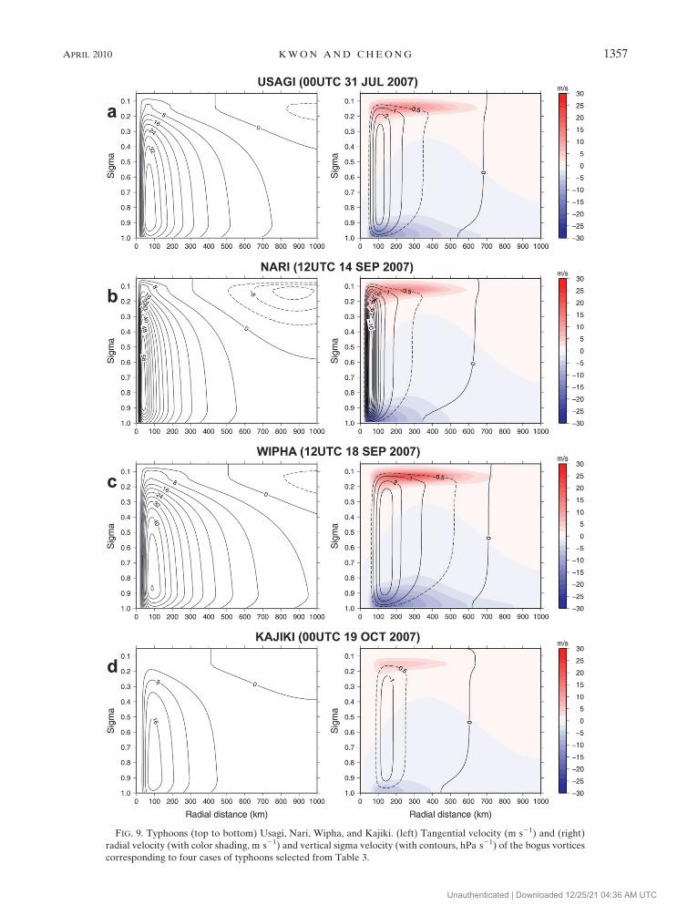
FIG. 9. Typhoons (top to bottom) Usagi, Nari, Wipha, and Kajiki. (left) Tangential velocity (m s21) and (right)

radial velocity (with color shading, m s21) and vertical sigma velocity (with contours, hPa s21) of the bogus vortices

corresponding to four cases of typhoons selected from Table 3.



available from the official Web sites of the RSMC (avail-

able online at http://www.jma.go.jp/jma/jma-eng/jma-

center/rsmc-hp-pub-eg/trackarchives.html) and the Joint

Typhoon Warning Center (JTWC; available online at

http://www.usno.navy.mil/NOOC/nmfc-ph/RSS/jtwc/best_

tracks/). In this study, the information from the RSMC is

used. All other parameters associated with the TC ini-

tialization are automatically determined based on these

values. Not any form of tuning or specification for in-

dividual TC is intervened during the forecasts.

The new TC initialization scheme is applied to the

track and intensity prediction of four TCs developed in

the western North Pacific and East China Sea in 2007:

Typhoons Nari, Usagi, Wipha, and Kajiki. For the case

of Typhoon Kajiki, the predictions of the operational

centers were found to be extremely poor both in the

track and intensity. The information reported from

RMSC on these TCs, which is used as basic input in the

initialization scheme, is presented in Table 3. The nu-

merical model adopted for the prediction of the TCs is

version 3.0 of the Weather Research and Forecasting

(WRF) model, whose resolutions are set at 12 km and 27

layers in horizontal and vertical directions, respectively.

The pressure at the model top is given at 50 hPa, and the

horizontal size of the model is approximately 358 3 358.

The total number of horizontal grids is set 281 3 251 for

all cases. The physical process options are the WSM

6-class for the microphysics (Hong and Lim 2006), the

Kain–Fritsch scheme for cumulus parameterization

(Kain and Fritsch 1990), and the Yonsei University

(YSU) package for PBL (Hong et al. 2006). The Na-

tional Centers for Environmental Prediction (NCEP)

Final Analyses (FNL) global analysis is used as the ini-

tial data, which is provided with the resolution of 18 3 18

at 26 vertical layers. For better representation of the

bogus vortex structure, the FNL data are interpolated to

produce higher-resolution global data of 0.1758 3 0.1758,

which is subject to high-order spectral filtering to get the

basic field and the disturbance for the TC initialization.

A part of the global high-resolution FNL data corre-

sponding to the model area is picked up as the initial

condition of the WRF model.

Before showing the simulation results, the procedure

of the TC initialization in Fig. 1 applied to the case of

Nari is illustrated in Fig. 10. The parameters that are

used to shape the bogus vortex were determined as

suggested in each step of Fig. 1. Compared to the global

analysis, the intensified vortex is identifiable in the ve-

locity map. A properly established bogus vortex would

result in a smooth time evolution of the prognostic

variables without giving a spurious jump or initial shock.

To see the possibility of a spurious jump in the begin-

ning of the time stepping, the temperature difference

between model output and the temperature deviation

obtained from geopotential using hydrostatic balance

equation was monitored in the initial 6 h. Such an ex-

ample for the case of Nari is illustrated in Fig. 11, where

two radial locations were selected: one is inside and the

other is outside the eyewall. The temperature difference

is found to vary in almost monotonic way or smoothly

over the vertical domain for both cases except that in the

middle layers inside the eyewall (r # 50 km) a rather

steep variation for about 20–30 min is observed. It may

be implied by this that the hydrostatic balance in the

bogus vortex is not quite appropriate near the TC center

whereas it proves to be a reasonable approximation

away from the center. It is not believed, however, that

the appearance of short period variation contaminates

the whole prediction of the TC. What is considered

important is the smooth transition of the initial vortex to

the nonhydrostatic regime without producing long-

lasting noisy fluctuations. It is not our intention to assert

that the less noise in the initial state is evidence of the

perfect representation of the TC of interest. From the be-

havior of the temperature, it may be stated that the sec-

ondary circulation on the radial-vertical plane was fairly

well organized in the bogus vortex.

The model is integrated for 48 h with the given initial

condition of bogus vortex. For each TC, several fore-

casts are carried out that start with their own initial

bogus vortex. To see the forecast improvement ach-

ieved from the new TC initialization, the forecasts us-

ing the same analysis but without the TC initialization

were also performed. The typhoon center was identi-

fied using the algorithm suggested by Kang and Cheong

(2001). First of all, the structures of the some variables

simulated with or without the TC initialization were

compared for the case of Typhoon Nari at 0000 UTC 14

September 2007. Figures 12 and 13 represent the geo-

potential deviation, temperature deviation, and the

meridional and zonal velocities at the initial time and

12 h after the time integration, respectively. As a result

of the TC initialization, the strong vortices and well-

organized temperature perturbation have been formed

as can be seen in Fig. 12. In Fig. 13 the strong vortexlike

structure is not developed even at 12 h after the time in-

tegration in the case without TC initialization. On the

other hand, the strong vortex was further intensified in the

case of TC initialization, as was similar to the observation.

Figure 14 presents the track forecasts of Typhoon Nari

along with the observation (best track of RSMC). It is

clearly seen that the forecasts with the TC initialization

show more improvement compared to the forecasts

without it. The tracks predicted with the TC initializa-

tion closely follow the best track for all cases shown in

this figure although the speed is somewhat different



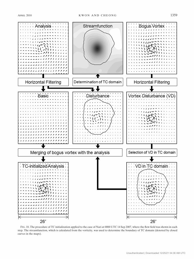
FIG. 10. The procedure of TC initialization applied to the case of Nari at 0000 UTC 14 Sep 2007, where the flow field was shown in each

step. The streamfunction, which is calculated from the vorticity, was used to determine the boundary of TC domain (denoted by closed

curves in the maps).



from the observation. It is worthy to note that the sim-

ulation without the TC initialization of 0000 UTC

15 September provided the track forecast of the north-

westward-moving direction while the observed track is

northeastward. Not shown, the forecasts with TC ini-

tialization for other cases also revealed similar im-

provements in track prediction over the forecasts

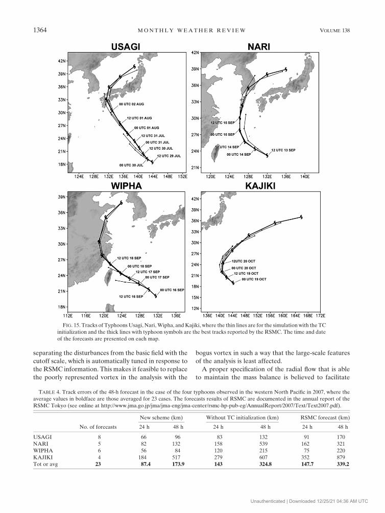
without it. The 48-h forecast track with a 12-h interval

for the cases Usagi, Nari, Wipha, and Kajiki are pre-

sented along with the observed tracks in Fig. 15. The

forecast tracks are well compared with the observed

tracks for all the cases. No significant westward or

eastward bias is shown, but the difference in moving

speed can be seen. Table 4 presents the average track

errors of the forecasts for each typhoon along with the

track errors of the RSMC operational forecasts. Among

the four typhoons cases, the smallest error was found to

be 84 km (48 h)21 for Wipha whereas the largest was

517 km (48 h)21 for Kajiki. The averaged track error of

total 23 cases for 4 typhoons was 173.9 km (48 h)21,

which was smaller than the errors provided by oper-

ational centers by about 165.3 km (48 h)21 (corre-

sponding to an approximate 49% improvement). It is

noticeable that in some cases the track forecasts without

a bogus vortex were better than the RSMC forecasts. In

Fig. 16, the time variation of the minimum surface pres-

sure (or central pressure), which is often used to repre-

sent the intensity, is presented for Typhoon Nari. The

difference from the observation increases almost mono-

tonically with time. The minimum surface pressure of

the forecasts with the TC initialization exhibits the time

evolution very close to the observation whereas it is not

the case for the forecasts without it. The forecast error in

the case without bogusing is as large as 30 hPa (48 h)21,

as can be seen for 0000 UTC 14 September 2007. The

root-mean-squared errors in the minimum surface pres-

sure are given in Table 5. The 48-h forecast errors in the

case with TC initialization are reduced by about 53%

and 55% compared to the cases without TC initializa-

tion and the forecasts of the operational center at RSMC,

respectively.

5. Discussion and conclusions

In this study a TC initialization method for the track

and intensity prediction was presented, where the ide-

alized three-dimensional bogus vortex of axisymmetry

was incorporated. The bogus vortex of empirical for-

mulas was constructed in a systematic way based on the

observed and simulated structures, where three balances

among variables were taken into consideration: the

gradient wind balance, the hydrostatic balance, and the

mass balance. All variables of the bogus vortex are

completely determined in analytic functions on input of

the basic four parameters issued by RSMC. To tightly

match the data over which the bogus vortex will replace

the disturbance field, two additional parameters (hinge

variables) were added to the RSMC parameters: the

ambient mean surface pressure and the averaged tem-

perature at the surface pressure level. Since the six pa-

rameters explicitly include the information about the

size and intensity, the bogus vortex faithfully reproduces

the important features specific to the tropical cyclone of

interest.

The new TC initialization method with the bogus

vortex requires the decomposition of disturbances and

the basic field from the analysis data, as is practiced in

the GFDL method. However, the streamfunction was

used in this study instead of the velocity fields at the time

FIG. 11. Time evolution of the temperature difference for the

initial 6 h, T2 2 T1(K), where T1 is the model output and T2 is

the hydrostatic temperature calculated from the geopotential

field in the case of Typhoon Nari at 0000 UTC 14 Sep 2007. The

temperature difference was averaged for (a) r # 50 km and

(b) 50 km , r , 300 km.



FIG. 12. East–west cross section of initial fields of (a) the geopotential deviation, (b) the temper-

ature deviation, (c) meridional velocity, and (d) zonal velocity of Typhoon Nari at 0000 UTC 14 Sep

2007, where the left (right) column is the case without (with) the TC initialization. Units for (a)–(d) are

m2 s22, K, m s21, and m s21, respectively.



FIG. 13. As in Fig. 12, but the fields are at 12 h after time integrations.



of scale separation using a filter. In this step, the DFS

high-order filter was used, which is computationally ef-

ficient and ensures a sharp cutoff at wanted horizontal

scale. The TC-scale disturbances are replaced by the

bogus vortex using a matching function that was also

filtered with the same filter used to eliminate the large-

scale component.

The new TC initialization scheme was applied to the

track and intensity forecasts of typhoons observed in

2007 over the western North Pacific and East China Sea.

As the forecast model the regional WRF v3.0 was used,

where the horizontal and vertical resolutions were set at

12 km and 27 layers, respectively. The selected cases

were Typhoons Usagi, Nari, Wipha, and Kajiki, for which

the official forecasts issued by operational centers (e.g.,

the RSMC), were found to be much poorer than the usual

cases. The track errors with the new scheme were found

to be much smaller than the forecasts without TC ini-

tialization by about 46%. The improvement over the op-

erational center at RSMC reached about 49%. The errors

of the minimum pressure were also reduced by about 55%

compared to the operational forecasts of the RSMC.

Among several factors included in the new scheme

that seem to have contributed to the forecast improve-

ment, the balances among variables and a sharp cutoff

filter are considered to be the most important. The im-

balance among variables of the bogus vortex may cause

an abrupt change in the TC intensity even within the first

few hours after time integration (e.g., Chou and Wu

2008; Wang et al. 2008). These imbalances seem to

produce systematic bias in the forecast model: in most

cases, the initial jump or drop of the central pressure

continues to exist during the whole period of time in-

tegration. The filter adopted in this study is capable of

FIG. 14. Tracks of Typhoon Nari simulated with (solid circle) and without (solid square) TC initialization, and of

the observation (open circle), where the symbols are indicated with a 6-h interval. Four sets of forecasts are shown

with a 12-h separation from 0000 UTC 14 Sep to 1200 UTC 15 Sep 2007.



separating the disturbances from the basic field with the

cutoff scale, which is automatically tuned in response to

the RSMC information. This makes it feasible to replace

the poorly represented vortex in the analysis with the

bogus vortex in such a way that the large-scale features

of the analysis is least affected.

A proper specification of the radial flow that is able

to maintain the mass balance is believed to facilitate

FIG. 15. Tracks of Typhoons Usagi, Nari, Wipha, and Kajiki, where the thin lines are for the simulation with the TC

initialization and the thick lines with typhoon symbols are the best tracks reported by the RSMC. The time and date

of the forecasts are presented on each map.

TABLE 4. Track errors of the 48-h forecast in the case of the four typhoons observed in the western North Pacific in 2007, where the

average values in boldface are those averaged for 23 cases. The forecasts results of RSMC are documented in the annual report of the

RSMC Tokyo (see online at http://www.jma.go.jp/jma/jma-eng/jma-center/rsmc-hp-pub-eg/AnnualReport/2007/Text/Text2007.pdf).

No. of forecasts

New scheme (km) Without TC initialization (km) RSMC forecast (km)

24 h 48 h 24 h 48 h 24 h 48 h

USAGI 8 66 96 83 132 91 170

NARI 5 82 132 158 539 162 321

WIPHA 6 56 84 120 215 75 220

KAJIKI 4 184 517 279 607 352 879

Tot or avg 23 87.4 173.9 143 324.8 147.7 339.2



the vertical motion especially near the center. In the

absence of either the inflow or outflow, the vertical mo-

tion may not be organized into the magnitude sufficient to

develop the TC. The success of the new scheme for the

TC track and intensity prediction in a variety of ranges in

horizontal scale and intensity seems to have been ach-

ieved by the flexibility of the bogus vortex whose vertical

and horizontal scale are specified automatically on input

of the RSMC information. Considering that there is

a certain level of uncertainty in SST, which plays a sig-

nificant role to the movement as well as development, the

magnitude of the errors in both track and intensity is

thought to be surprisingly small. It is expected to see

further reduced errors than the scores in Tables 4 and 5 if

the new scheme is applied to more TCs because the ty-

phoons adopted for validation in this study were the cases

of poor forecast score for operational centers.

The asymmetric component was not included in the bo-

gus vortex unlike the GFDL method under the assumption

that the important part of the asymmetric component (or

beta gyre) remains in the basic field. To see whether this

assumption is reasonable, the FNL analysis field, both

FIG. 16. Time variation of the minimum surface pressure of selected four cases of Typhoon Nari simulated with

(solid circle) and without (solid square) TC initialization, and of the observation (open circle), where the symbols

are indicated with a 6-h interval. Four sets of forecasts are shown with a 12-h separation from 0000 UTC 14 Sep to

1200 UTC 15 Sep 2007.

TABLE 5. The root-mean-squared errors of the 48-h forecasts for the minimum surface pressure averaged for the cases as in Table 4.

No. of forecasts

New scheme (hPa) Without TC initialization (hPa) RSMC forecast (hPa)

24 h 48 h 24 h 48 h 24 h 48 h

USAGI 8 16.4 11.3 31.0 17.5 7.9 11.5

NARI 5 6.0 8.0 42.5 20.0 25.4 28.9

WIPHA 6 10.9 7.3 34.1 19.2 26.8 29.4

KAJIKI 4 7.6 14.1 48.2 33.0 22.6 26.7

Tot or avg 23 11.2 10.0 37.3 21.2 19.2 22.4



with and without the bogus vortex, was analyzed in some

detail. Our attention was restricted to the disturbance

field because the bogus vortex is designed in order to

replace only the disturbance field of the analysis data.

It was revealed that there was no clear indication of

a well-organized column of asymmetric component in

the disturbance field. In some cases, a well-organized

wavenumber-1 component in azimuthal direction was

detected. However, this asymmetric structure was only

confined to a certain vertical level, without giving a ver-

tically extended structure. In the same context, the TCs

simulated with the ideal 3D bogus vortex were also an-

alyzed in detail. The results revealed that the disturbance

fields of the 6-, 12-, and 24-h forecast did not exhibit

a well-established wavenumber-1 component, either.

Therefore as long as the vertically extended asym-

metric component is considered to be significant, it was

not necessary to include the asymmetric component in

the bogus vortex.

Acknowledgments. This work was funded by the Korea

Meteorological Administration (KMA) Research and

Development Program under Grant CATER 2007-2206.

The useful comments from the anonymous reviewers are

acknowledged. The authors would like thank Professor

Song-You Hong for helpful discussions. They also want

to express appreciation to Sung-Wook Park, Ja-Rin Park,

Hyun-Jun Han, and Hyun-Gyu Kang for preparing the

figures and supporting them with the computing system.

REFERENCES

Anthes, R. A., 1982: Tropical Cyclones: Their Evolution, Structure,

and Effects. Amer. Meteor. Soc., 208 pp.

Ausman, M., 1959: Some computations of the inflow angle in

hurricanes near the ocean surface. Research Rep., Depart-

ment of Meteorology, University of Chicago, 19 pp.

Bender, M. A., I. Ginis, R. Tuleya, B. Thomas, and T. Marchok,

2007: The operational GFDL coupled hurricane–ocean pre-

diction system and a summary of its performance. Mon. Wea.

Rev., 135, 3965–3989.

Braun, S. A., M. T. Montgomery, and Z. Pu, 2006: High-resolution

simulation of Hurricane Bonnie (1998). Part I: The organiza-

tion of eyewall vertical motion. J. Atmos. Sci., 63, 19–42.

Carr, L. E., III, and R. L. Elsberry, 1992: Analytical tropical cy-

clone asymmetric circulation for barotropic model initial

conditions. Mon. Wea. Rev., 120, 644–652.

Chan, J. C.-L., and R. T. Williams, 1987: Analytical and numerical

study of the beta-effect in tropical cyclone motion. Part I: Zero

mean flow. J. Atmos. Sci., 44, 1257–1265.

Cheong, H.-B., I.-H. Kwon, T.-Y. Goo, and M.-J. Lee, 2002: High-

order harmonic spectral filter with the double Fourier series

on a sphere. J. Comput. Phys., 177, 313–335.

——, ——, and ——, 2004: Further study on the high-order double

Fourier series spectral filtering on a sphere. J. Comput. Phys.,

193, 180–197.

Chou, K.-H., and C.-C. Wu, 2008: Typhoon initialization in a

mesoscale model—Combination of the bogused vortex and

the dropwindsonde data in DOTSTAR. Mon. Wea. Rev.,

136, 865–879.

Frank, W. M., 1977: The structure and energetics of the tropical cy-

clone. Part I: Storm structure. Mon. Wea. Rev., 105, 1119–1135.

Fujita, T., 1952: Pressure distribution within typhoon. Geophys.

Mag., 23, 437–451.

Gray, W. M., 1979: Hurricanes: Their formation, structure, and

likely role in the tropical circulation. Meteorology over the

Tropical Oceans, D. B. Shaw, Ed., Royal Meteorology Society,

155–218.

Grijn, G. V. D., J. E. Paulsen, F. Lalaurette, and M. Leutbecher, 2005:

Early medium-range forecasts of tropical cyclones. ECMWF

Newsletter, No. 102, ECMWF, Reading, United Kingdom, 7–14.

Harper, B. A., and G. J. Holland, 1999: An updated parametric model

of the tropical cyclone. Preprints, 23rd Conf. on Hurricane and

Tropical Meteorology, Dallas, TX, Amer. Meteor. Soc., 893–896.

Holland, G. J., 1980: An analytic model of the wind and pressure

profiles in hurricanes. Mon. Wea. Rev., 108, 1212–1218.

——, 1983: Tropical cyclone motion: Environmental interaction

plus a beta effect. J. Atmos. Sci., 40, 328–342.

——, and R. T. Merrill, 1984: On the dynamics of tropical cyclone

structural changes. Quart. J. Roy. Meteor. Soc., 110, 723–745.

Hong, S.-Y., and J.-O. J. Lim, 2006: The WRF single-moment

6-class microphysics scheme (WSM6). J. Korean Meteor. Soc.,

42, 129–151.

——, Y. Noh, and J. Dudhia, 2006: A new vertical diffusion

package with an explicit treatment of entrainment processes.

Mon. Wea. Rev., 134, 2318–2341.

Iwasaki, T., H. Nakano, and M. Sugi, 1987: The performance of

a typhoon track prediction model with convective parame-

terization. J. Meteor. Soc. Japan, 65, 555–570.

Kain, J. S., and J. M. Fritsch, 1990: A one-dimensional entraining/

detraining plume model and its application in convective pa-

rameterization. J. Atmos. Sci., 47, 2784–2802.

Kang, M.-K., and H.-B. Cheong, 2001: Oscillation of separation

distance between paired typhoon-scale vortices. J. Meteor.

Soc. Japan, 79, 967–983.

Kurihara, Y., M. A. Bender, and R. J. Ross, 1993: An initialization

scheme of hurricane models by vortex specification. Mon.

Wea. Rev., 121, 2030–2045.

——, ——, R. E. Tuleya, and R. J. Ross, 1995: Improvements in the

GFDL hurricane prediction system. Mon. Wea. Rev., 123,

2791–2801.

Kwon, H.-J., 2002: Development of medium-range ensemble fore-

cast technique in typhoon model (in Korean, with the summary

in English). Improvement of Medium-Range Forecast System,

H.-B. Cheong, Ed., Korea Meteorological Administration,

149–234.

Leslie, L. M., and G. J. Holland, 1995: On the bogussing of tropical

cyclones in numerical models: A comparison of vortex pro-

files. Meteor. Atmos. Phys., 56, 101–110.

Liu, Y., D.-L. Zhang, and M. K. Yau, 1999: A multiscale numerical

study of Hurricane Andrew (1992). Part II: Kinematics and

inner-core structures. Mon. Wea. Rev., 127, 2597–2616.

Mathur, M. B., 1991: The National Meteorological Center’s quasi-

Lagrangian model for hurricane prediction. Mon. Wea. Rev.,

119, 1419–1447.

Peng, M., L. Xie, and L. J. Pietrafesa, 2006: Tropical cyclone in-

duced asymmetry of sea level surge and fall and its pre-

sentation in a storm surge model with parametric wind fields.

Ocean Modell., 14, 81–101.



Phadke, A. C., C. D. Martino, K. F. Cheung, and S. H. Houston,

2003: Modeling of tropical cyclone winds and waves for

emergency management. Ocean Eng., 30, 553–578.

Press, W. H., S. A. Teukolsky, W. T. Vetterling, and B. P. Flannery,

1992: Numerical Recipes in FORTRAN. 2nd ed. Cambridge

University Press, 963 pp.

Pu, Z. X., and S. A. Braun, 2001: Evaluation of bogus vortex

techniques with four-dimensional variational data assimila-

tion. Mon. Wea. Rev., 129, 2023–2039.

Richardson, D. S., and Coauthors, 2008: Verification statistics and

evaluation of ECMWF forecasts in 2007–2008. ECMWF Tech.

Memo. 578, 45 pp.

Serrano, E., and P. Unden, 1994: Evaluation of a tropical cyclone

bogusing method in data assimilation and forecasting. Mon.

Wea. Rev., 122, 1523–1547.

Smith, R. B., 1993: A hurricane beta-drift law. J. Atmos. Sci., 50,

3213–3215.

Thu, T. V., and T. N. Krishnamurti, 1992: Vortex initialization for

typhoon track prediction. Meteor. Atmos. Phys., 47, 117–126.

Tremolet, Y., 2005: Incremental 4D-Var convergence study.

ECMWF Tech. Memo. 469, 36 pp.

Wang, D., X. Liang, Y. Zhao, and B. Wang, 2008: A comparison of

two tropical cyclone bogussing schemes. Wea. Forecasting, 23,

194–204.

Williams, R. T., and J. C.-L. Chan, 1994: Numerical studies of the

beta effect in tropical cyclone motion. Part II: Zonal mean

flow effects. J. Atmos. Sci., 51, 1065–1076.

Zhang, X., Q. Xiao, and P. J. Fitzpatrick, 2007: The impact of

multisatellite data on the initialization and simulation of

Hurricane Lili’s (2002) rapid weakening phase. Mon. Wea.

Rev., 135, 526–548.

Zou, X., and Q. Xiao, 2000: Studies on the initialization and sim-

ulation of a mature hurricane using a variational bogus data

assimilation scheme. J. Atmos. Sci., 57, 836–860.



Tropical Cyclone Initialization with a Spherical High ...

Documents

Transcript of Tropical Cyclone Initialization with a Spherical High ...