TRIPLE BOTTOM LINE AND LIFE CYCLE COST ASSESSMENTS

OF SUSTAINABLE RESOURCE MANAGEMENT IN BOSTON, MA

A Thesis Presented

by

Joseph Farah

To

The Department of Civil and Environmental Engineering

in partial fulfillment of the requirements

for the degree of

Masters of Science

in

Civil Engineering

in the field of

Environmental Engineering

Northeastern University

Boston, MA

July 2008

i

ABSTRACT

Urban planners today are facing a multitude of problems with the prevailing paradigm of

development. Apart from being hydrologically unbalanced, and operating on a “fast-

conveyance” premise, large cities suffer from high levels of greenhouse gas emissions

and inefficient management of resources. Realizing the need for a different paradigm of

development, this study examines the feasibility of a new urban management approaches

based on the concepts of “Total Hydrologic Balance” and “Sustainability”. Water

conservation and reuse, energy conservation, vegetated roofs, decentralized water

management in semi-autonomous urban clusters, and integrated resource management

were investigated in multiple configurations and assessed for benefits on a “Triple

Bottom Line” basis. Green roofs were studied for water retention, runoff reduction and

building insulation and were found to be effective in reducing runoff from the one-year

storm. However, for larger design storms there’s a need to couple green roofs with other

tools that reduce directly connected impervious areas. For water reclamation, facilities

using biological nutrient removal and yielding a high quality reusable effluent were

proposed inside the urban ecoblocks with their cost estimated from construction curves.

Water and energy conservation were thoroughly dealt with and broken down to direct and

indirect ways to conserve, while proposing low flow fixtures and energy efficient

appliances with no or minimal additional cost. Anaerobic digestion of sludge and heat

extraction from wastewater were also considered as renewable sources of energy. A

“Life-Cycle Cost Analysis” was also used in order to determine the economic viability

and applicability of each proposed alternative. Such analysis revealed that sustainable

management is feasible for different scales of cluster and various land use compositions.

Alternatives centered on water management or green roofs only were not feasible on their

own while comprehensive alternatives using a holistic approach and plans incorporating

energy conservation were the most beneficial. Land use and population density were

analyzed for their effects on the different scenarios. The results suggested that the

payback period was not much affected by those parameters while the net present worth

showed it highest values at 55-70% developed land cover and a population density in the

range of 6000-9000 persons/km2.

ii

ACKNOWLEDGMENTS

This study could not have been completed were it not for the contribution of various

people. First and foremost, I would to gratefully acknowledge the extensive support and

invaluable advice of my research advisor Professor Vladimir Novotny, who is not only a

leading figure in the fields of water quality and environmental engineering but also an

inspiring supervisor. Gratitude also to Dr. Annalisa Onnis Hayden and Professor Ferdi

Hellweger for their assistance in obtaining necessary data and clearing out ambiguities in

this report. I also greatly appreciate the encouragement of my colleagues and friends at

the Department of Civil and Environmental Engineering, mainly David Bedoya, Indrani

Ghosh, Carla Cherchi, Nehreen Majed, Vanni Bucci and David Doran. Many thanks as

well to my parents Nassim and Layla Farah for always believing in me. And finally I

can’t conclude without thanking God for giving me the strength and the will to finish this

study and move on to greater things.

iii

TABLE OF CONTENTS Abstract……………………………………………………………………………………. i Acknowledgments………………………………………………………………………… ii Table of Contents…………………………………………………………………………. iii List of Abbreviations……………………………………………………………………... v List of Tables……………………………………………………………………………… vi List of Figures……………………………………………………………………………... vii CHAPTER 1: INTRODUCTION………………………………………………………... 1 1.1 Problem Statement…………………………………………………………………. 1 1.2 Description of this Study…………………………………………………………....10 CHAPTER 2: STUDY AREA……………………………………………………………. 13 CHAPTER 3: WATER AND ENERGY CONSERVATION………………………….. 19 3.1 Water Conservation………………………………………………………………... 19 3.1.1 Toilets and Urinals……………………………………………………………….. 22 3.1.2 Faucets and Taps………………………………………………………………….. 22 3.1.3 Showerheads……………………………………………………………………….. 23 3.1.4 Dishwashers and Washing Machines………………………………………….. 23 3.2 Energy Conservation……………………………………………………………….. 25 3.2.1 Indirect Energy Savings……………………………………………………………26 3.2.2 Direct Energy Savings……………………………………………………………. 27 CHAPTER 4: VEGETATED ROOFS…………………………………………………...31 4.1 Implementation of Green Roofs in this Study……………………………………... 31 4.2 Water Retention by Green Roofs…………………………………………………... 36 4.3 Peak Flow and Runoff Reduction by Green Roofs………………………………… 38 4.4 Direct Energy Savings from Green Roofs…………………………………………. 43 4.5 Cost Considerations………………………………………………………………... 46 CHAPTER 5: WATER SUPPLY, RECLAMATION AND REUSE…………………..48 5.1 Water Supply………………………………………………………………………. 48 5.2 Wastewater Treatment and Reuse…………………………………………………. 50 CHAPTER 6: ALTERNATIVE ENERGY & IRM……………………………………..54 6.1 Anaerobic Digestion and Biogas Production………………………………………. 54 6.2 Heat Extraction…………………………………………………………………….. 57 CHAPTER 7: TBL & LCC ASSESSMENTS…………………………………………...60 7.1 Triple Bottom Line Assessment…………………………………………………….60 7.2 Life Cycle Cost Assessment……………………………………………………….. 65 7.2.1 Vegetated Roofs Only……………………………………………………………... 67 7.2.2 Vegetated Roofs and Energy Conservation……………………………………. 71 7.2.3 Vegetated Roofs, Ecoblocks, IRM, Energy and Water Conservation………. 73

iv

7.2.4 Vegetated Roofs, Ecoblocks, Water Conservation and Reuse……………......75 7.2.5 No Vegetated Roofs………………………………………………………………...77 7.3 Analysis and Discussion…………………………………………………………… 78 CHAPTER 8: CONCLUSIONS AND FINAL THOUGHTS…………………………...86 APPENDIX A: EXTRACTS FROM IPCC REPORT 2007…………………………….93 APPENDIX B: LAND USE CODE DEFINITIONS……………………………………. 95 APPENDIX C: DATA ON ENERGY REQUIREMENTS FOR WATER CONVEYANCE AND TREATMENT……………………………………………………...96 APPENDIX D: 2005-2007 PRECIPITATION SERIES FOR BOSTON WITH RETAINED DEPTH BY GREEN ROOFS……………………………………………98 REFERENCES……………………………………………………………………………. 107

v

LIST OF ABBREVIATIONS BFA Building Footprint Area BNR Biological Nutrient Removal CFL Compact Fluorescent Lights DES Direct Energy Savings GHG Greenhouse Gases GRA Green Roofs Area IES Indirect Energy Savings IRM Integrated Resource Management LCC Life-Cycle Cost LCCA Life-Cycle Cost Assessment NPW Net Present Worth PBP Payback Period TBL Triple Bottom Line WRF Water Reclamation Facility WSC Water Saved by Conservation WWTP Wastewater Treatment Plant YWR Yearly Water Retention

vi

LIST OF TABLES Table Description Page 2.1 Areas of the Ecoblocks 15 2.2 Population Estimates of the Ecoblocks 16 2.3 Aggregated Codes for each Land Use Category 17 2.4 Land Use Composition of the Ecoblocks 18 3.1 Feasible Water Savings in Residential Households 24 3.2 Feasible Water Savings in Commercial Buildings 24 3.3 Water Saved by Conservation 25 3.4 Energy Requirement for Water-Related Works 26 3.5 Indirect Energy Savings 27 3.6 Direct Energy Saving for Water Conserving Fixtures and Machines 28 3.7 Equivalent Wattage for CFLs for the Same Light Output 29 3.8 Energy Savings Provided by CFLs 30 4.1 BFA and GRA of Ecoblocks 36 4.2 Water Retention Computations 37 4.3 Yearly Water Retention by Green Roofs along with IES 38 4.4 Curve Numbers with Traditional and Green Roofs 39 4.5 Peak Flow Differences between Traditional and Green Roofs 40 4.6 Runoff Differences between Traditional and Green Roofs 41 4.7 Computation of Average ΔT 44 4.8 Yearly Energy Savings Provided by Green Roofs 45 4.9 Total Direct Energy Savings in Ecoblocks 46 4.10 Cost of Green Roofs 47 5.1 Typical Distribution of Residential Water Use 48 5.2 Typical Flow Rates for Commercial and Institutional Buildings 49 5.3 Water Supply Flow Rate 50 5.4 Effluent Quality Provided by BNR 51 5.5 Capital Costs of Water Reclamation Facilities and Yearly 53 6.1 Energy from Anaerobic Digestion of Sludge 57 6.2 Heat Extracted from Sewage 59 7.1 Environmental Benefits 61 7.2 Social Benefits 62 7.3 Economic Benefits 64 7.4 Economic Analysis with Green Roofs Only 68 7.5 Sensitivity Analysis with Green Roofs Only Scenario 70 7.6 Economic Analysis for an Energy-Centric Scenario 72 7.7 Economic Analysis for a Comprehensive Scenario 74 7.8 Economic Analysis for a Water-Centric Scenario 76 7.9 Economic Analysis with No Green Roofs 77

vii

LIST OF FIGURES Figure Description Page 1.1 US Anthropogenic Greenhouse Gas Emissions 5 1.2 Traditional Water Management in Cities 8 1.3 Proposed Water Management Approach 9 1.4 Benefits to be Quantified using a TBL Assessment 11 2.1 Ecoblock 1 13 2.2 Base Ecoblocks in the Study 14 2.3 Land Use in South Boston 19 4.1 Green Roof Tested at the University of Virginia 33 4.2 Building Footprints with a Zoom on Ecoblock 1 35 4.3 Retention Percentages for Different Categories of Rainfall 37 4.4 %Reduction in Runoff versus the Rooftop Cover 42 5.1 Construction Cost Curve for BNR Water Reclamation Facilities 52 6.1 Integrated Resource Management in BC 55 6.2 Stages of Anaerobic Digestion 56 6.3 Thermodynamic Cycle of Heat Extraction 58 7.1 Incremental Cash Flow Diagram 66 7.2 NPW of the Five Scenarios in the Ecobloks 80 7.3 Payback Period of the Three Feasible Scenarios in the Ecoblocks 80 7.4 NPW versus % Developed 82 7.5 PBP versus % Developed 82 7.6 NPW versus Population Density 83 7.7 PBP versus Population Density 83

1

CHAPTER 1

INTRODUCTION

1.1- Problem Statement Most of today’s cities are marred by the corollaries of a flawed pattern of growth that

inflicted upon environmental, social and economic health, hydrology, and water

resources. Based on recommendations from the Wingspread workshop (Racine,

Wisconsin 2006), Novotny and Brown (2007) emphasized the need to adopt a new model

for urban development called the “Fifth Paradigm of Urbanization”. The way in which

man has approached his relationship with his natural environment and water resources

has evolved in five paradigms. At first man enslaved nature and dumped his waste in

unpaved streets waiting for them to be washed off by rain and snowmelt. The people of

the first A.D. centuries used streams for irrigation and transportation and groundwater for

potable water supplies.

It took a few centuries before the engineered practices of storage and conveyance became

widespread, as city populations and ensuing water demands grew. Combined sewers that

emerged in the 18th century collected wastewater and polluted runoff and quickly

conveyed them to streams and lakes, effects that have carried over to the present day. As

man continued to stress the available water bodies and relay his problems to nature, he

created a myriad of problems. Outbreak of pandemics and diseases from the very body

that he uses as an outfall for waste and an intake of water have compelled man to seek a

different model. By the beginning of the 20th century, control of point sources of

pollution was being exerted through a massive practice of building wastewater treatment

2

plants. That, however, did not address the issue of polluted runoff. With the increase in

impervious surfaces and the quest for more agricultural yields, urbanization and nonpoint

source pollution prevented any major improvements in the quality of water. Therefore the

need for an approach which deals with diffuse pollution developed and resulted in the

very recent ongoing “end-of-pipe control” or fourth paradigm. A major milestone in this

paradigm was the Clean Water Act of 1972 which emphasized the need to restore the

integrity of waterbodies and protect them against urban and agricultural runoff. That

spurred an intense application of Total Maximum Daily Load (TMDL) and Use

Attainability Analysis (UAA) studies. Undeniably, the current paradigm had some

success in abating waterborne diseases and helped many rivers regain their vitality.

Nonetheless, it failed in preventing the detrimental effects resulting from urbanization

and long distance water transfer.

Today’s urban hubs are hydrologically unbalanced. Impervious surfaces dominating the

landscape of cities have invariably altered the predevelopment hydrologic behavior.

Naturally, rainfall hits the surface or is intercepted by vegetation. It ponds into

depressions and a large portion (~30-40 %) is returned to the atmosphere via evaporation

and transpiration. The remaining portion runs off into streams and rivers or infiltrates into

the ground thereby recharging groundwater formations, which ultimately feed the

baseflow of rivers providing for their perenniality. In contrast, a typical city with its

impermeable streets, curbs and parking lots modifies this cycle by reducing evapo-

transpiration and infiltration on one hand and increasing surface runoff on the other. This

increase in surface runoff is exacerbated by the fact that the existing drainage systems

operate on a “fast-conveyance” premise. In other words, today’s characteristic “inlet-

3

sewer- catch basin” or “curb and gutter” drainage system is designed to quickly drain the

runoff from streets and lots and convey it to rivers or wastewater treatment plants

(WWTPs). Therefore peak flows from storms increase by a factor from 4 to 10 in an

urban setting (Novotny, 2003). The direct outcome manifested in increased recurrence of

urban flooding which in the future may be worsened by global climate changes, and the

increased frequency of storm surges. Water which should infiltrate to aquifers and

recharge rivers at its own pace is now being collected and quickly transferred out.

Consequently, urban streams have either lost or suffered a major blow in their baseflow

supply and some have turned from perennial to ephemeral. Several are even termed

“effluent dominated” or “effluent dependent” streams in that the major flow they receive

is the discharge from WWTPs or that the discharge is of relatively good quality that can

support aquatic life. For example, the Los Angeles River is now an ephemeral urban and

the Stony Brook in Boston is currently effluent-dominated. The drop in the groundwater

table due to the lack of infiltration may also cause subsidence of the soil bed and

endanger building foundations. This effect is most observed in the city of Boston,

especially the Back Bay area which was developed by filling into the waters of the Back

Bay and piling timber columns into the fill to serve as building foundations. A drop in the

groundwater table would cause the piles to rot, and that prompted the city of Boston to

use large volumes of fresh water to replenish the groundwater.

Moreover, another problem which has taken its toll on water resources is the long

distance transfer of water and sewage. Because of economy of scale and cost-

effectiveness, high capacity treatment plants were built to service large areas. As such

large pipe networks were needed and water / wastewater was being transferred for long

4

distances. This practice has led to flow-deprived source areas and effluent dominated

waters receiving the discharge from the large WWTP. For instance, the Deer Island

WWTP in Boston is the second largest treatment plant in the United States with a

network radius of 30 miles. Such large networks suffer from inflow of rainwater into the

system which can massively increase the volume of water being treated and add

unnecessary costs to the operator. Kate Bowditch (2007), project director at the Charles

River Watershed Association, Boston, noted that the amount of sewage being treated at

the Dear Island WWTP is nearly twice the amount that enters the system due to inflow

into the sewers and illicit stormwater discharges.

The impaired state of the urban environment, however, far transcends the dilemma of

improper water management to the realm of the atmosphere and greenhouse gas (GHG)

emissions. Perry McCarty (2008) singled out high CO2 levels as a major driver for

environmental policy makers in the near future and proposed radical changes in all

aspects of urban water, wastewater and energy management. The International Panel on

Climate Change (IPCC, 2007) assessed the changes in CO2 levels, sea levels, temperature

and snow cover over time. The panel noted that excessive fossil fuel usage and land use

changes were the major cause of elevated CO2 concentrations while agriculture was the

cause of increasing methane (CH4) and nitrous oxide (N2O) concentrations.

Concentrations of those three GHGs now “far exceed pre-industrial values determined

from ice cores spanning many thousands of years”. For instance, the atmospheric

concentration of CO2 in 2005 was measured to be 379 ppm increasing from the

preindustrial value of 280 ppm and exceeding any value in the preceding 650,000 years

(IPCC, 2007).

5

Such high GHG concentrations have been correlated with increased radiative forcing,

global air and ocean temperature, widespread reduction of the snow and ice cover and

rising global mean sea levels. Appendix A includes figures and graphs extracted from the

2007 IPCC report showing the aforesaid dramatic changes. IPCC (2007) also asserted

that “most of the observed increase in globally averaged temperatures since the mid-20th

century is very likely due to the observed increase in anthropogenic greenhouse gas

concentrations”, thus putting human activity at the forefront of the problem. Narrowing

down even further reveals that electricity is the major source of anthropogenic CO2

emissions. According to EPA (2007), electricity accounts for 33% of the carbon footprint

followed by transportation at 28% and sources such as wastewater treatment at 3%

(Figure 1.1).

Figure 1.1: US Anthropogenic Greenhouse Gas Emissions

(Source: US EPA Inventory of Greenhouse Gas Emissions and Sink 1990-2005, Feb. 2007)

6

The aforementioned drawbacks of current water/wastewater management practices,

coupled with the effects of population growth and global warming, could be solved by a

more sustainable paradigm, the fifth paradigm. This paradigm is still in the conceptual

phase and it’s yet to be adopted as a widespread right model of development [this study’s

greater aim is to contribute to the formulation of this paradigm]. The fifth paradigm can

be called “the paradigm of sustainability”. Sustainable development should “meet the

needs of the present without compromising the ability of future generations to meet their

needs” (Bruntland et al., 1987). Ensuring environmental sustainability is also among the

United Nations development goals for the millennium.

Novotny and Brown (2007) highlighted that sustainability can be achieved through a

holistic approach in water management, an approach concerned with optimizing the

whole rather than focusing on a specific component (drinking water, sewage, stormwater,

heat). This holistic approach can be materialized through the concept of “Total

Hydrologic Balance” whereby the reuse and recycling of water is maximized and the

amount of water leaving the system (loop) is minimized. In an exhaustive manner,

sustainability can be attained by:

- Implementing the concepts of smart green development: rain gardens, bioswales,

eco-roofs, ponds, underground storage tanks and pervious pavement to enhance

storage and infiltration within the watershed, recharge aquifers and minimize

subsidence. Such practices will reduce peaks flows and allow for storage of water

on site, which may be used for flow-augmentation in rivers.

7

- Reusing treated effluent for landscape irrigation and flushing toilets. Some

effluents are even of a quality comparable to drinking water and their treatment

facility is called a Water Reclamation Facility (WRF).

- Reduction of imperviousness and the restoration of green corridors planted with

coniferous trees that retain water. This will help mimic the natural hydrology of a

predeveloped natural system by increasing evapotranspiration and infiltration, and

provide habitat for different species. Green corridors also improve the air quality

and reduce noise pollution.

- Decentralizing wastewater treatment and clustering the city into smaller semi-

autonomous developments which may be termed “urban clusters” or “Ecoblocks”.

An urban cluster is a set of buildings and developments with a population in the

order of thousands. The cluster could be delineated by major streets or major

landscape features or it could be one large building. However, an urban cluster

has to be a hydrologically independent entity where water management in-situ is

maximized.

- Water and energy conservation practices at the building level using efficient home

appliance and equipment.

Ultimately, on a wider scale a green and sustainable approach should also incorporate:

- Reduction of energy consumption by building a robust system of public

transportation, electric buses and nonpolluting biofuels. Biofuels may be

produced from wastewater biosolids. Stockholm, Sweeden for example is

currently using biogas to power its bus network, gradually phasing out diesel-

powered buses. “Fortum Energi”, a Stockholm energy company also uses heat

8

pumps to extract heat from sewage and provide hot water to about 80,000

apartments. Making a resource out of waste, also called Integrated Resource

Management (IRM) has been recommended in the Capital Regional District

(CRD) of Victoria, BC (Aquatex, 2008).

- Remediating urban brownfields and using them as green space recreation.

- Restoring the baseflow in impaired urban streams. Some urban streams have been

buried in culverts under roads and sustainability suggests that they be daylighted.

Daylighting first order streams which became ephemeral, along with infiltration

enhancing pervious pavements and rain gardens, will restore their baseflow and

aquatic life. It will also facilitate the restoration of second and higher order

streams and make for an interconnected system.

Figures 1.2 and 1.3 below show the difference from a water management perspective

between today’s highly urbanized cities and proposed ecoblocks.

Figure 1.2: Traditional Water Management in Cities

9

Figure 1.3: Proposed Water Management Approach (Novotny, 2007)

The proposed approach in figure 1.3 - a rationale in the fifth paradigm - graphically

embodies the components of green sustainable hydrology and water management

outlined above, on both the cluster scale and the city scale. Not shown in the two figures

above though, are elements pertaining to reduction of GHG emissions. However,

reduction of water use and wastewater generation is in turn conducive to a solid reduction

in energy. As it will be shown in later sections, it takes great amounts of energy to treat,

supply and convey water. Wilson (2008) proposed that energy and electricity be saved

based on water management strategy since water and energy constitute a nexus, and as

such a “Total Hydrologic Balance” implicitly includes an energy balance component.

Looking at the bigger picture, a “Total Hydrologic Balance” is an offshoot from the more

general concept of sustainability, which has no definite standards at the moment (Wilson,

10

2008). Some standards such as LEED establish some water and energy efficient measures

but they falter at the prospect of measuring the holistic sustainability of a development.

Therefore, Novotny (2007) proposed that sustainability be evaluated within the context of

a “Triple Bottom Line” (TBL) Assessment. This assessment uses “society” and the

“environment” on top of the “economics” to evaluate the benefits of a development since

thinking only in terms of one bottom line, money, has had severe impacts. This means

that a development is sustainable in as much as it brings about environmental/ecological

protection and enhancement measures, enhances the quality of social life, and generates

revenues and savings over its life-cycle.

1.2- Description of this study

This research study will assess based on a TBL approach, the benefits and feasibility of

sustainable management in the city of Boston, a city riddled by the impacts of urban

development where first order streams such as the Stony Brook have been lost,

groundwater levels have been sinking, threatening the integrity of foundations in the

Back Bay area, and where water conservation and reuse is by no means widespread. This

study will investigate optimization of water and energy management at the building level

and at the scale of urban clusters. Proposed changes will have minimum impact on the

outside layout of the city. The reasoning behind this as termed by Speers (2007) is

“successive limited comparison”, which describes that policy makers usually consider

policies which differ from the ones in effect by a relatively small degree, thereby

reducing the number of alternatives to be considered. The city of Boston will be clustered

into ecoblocks different in size with each having its own water reclamation facility

(WRF). These facilities would use Biological Nutrient Removal (BNR) to treat the

11

influent wastewater and produce a high quality effluent suitable for reuse such as toilet

flushing, irrigation and streamflow augmentation. The costs of the WRF will be

calculated from construction curves provided by Carollo Engineers, a leading US

company in the construction and operation of wastewater treatment plants. Green roofs

will also be used on buildings inside ecoblocks with an assumption that they are

applicable on 70% of the roof area in the city of Boston. The green roof for this study is

an American Hydrotech vegetated roof with a lightweight roof garden mix provided by

ItSaul Natural LLC (subject of a modeling study conducted at the University of Georgia,

Athens, Georgia). The viability of using heat extraction from wastewater will also be

discussed in largely commercial areas.

Figure 1.4 shows the benefits that will be quantified for each ecoblock based on a TBL

assessment. Certainly sustainable development carries more benefits but the ones below

pertain only to the proposed water/energy conservation policies and elements in this

research study.

Figure 1.4: Benefits to be Quantified using a TBL Assessment

12

Savings from energy/water conservation will be tallied on a yearly basis and then a

comprehensive life-cycle cost assessment (LCCA) will be performed for each ecoblock

using the computed initial costs, yearly benefits and yearly expenses. The net present

worth (NPW) will be calculated along with the payback period (PBP) provided that the

alternative proves to be feasible.

Subsequently the objectives of this study are the following:

- Investigate whether sustainable resource management is economically feasible

and if optimization of water and energy consumption at the parcel or household

level would generate enough benefits to recover the investment in the WRF

and/or be able to produce appreciable environmental and social impacts.

- Study the effect of the characteristics of the ecoblock (land use, size, population)

– if any – on the calculated benefits.

- Analyze the results of using vegetated roofs within the framework of a stormwater

management policy on a watershed scale.

- Compare different management alternatives and determine the suitability of each.

13

CHAPTER 2

STUDY AREA

The imaginary urban clusters or ecoblocks in this study are located in the southern part of

the city of Boston and as shown in figure 2.2, bound by the mouth of the Charles River

and the Boston inner harbor. The ecoblocks were created by obtaining the GIS shapefiles

of the EOT roads and building footprints from MassGIS1, the commonwealth’s office of

geographic and environmental information within the Massachusetts Executive office of

Environmental Affairs. These GIS data layers, as well as all others in this study use a

Lambert Conformal Projection and a NAD83 Stateplane MA Mainland Coordinate

system. Using ArcMap in ArcView 9.1, clustering of buildings was performed using

major roads as the boundary lines between ecoblocks.

Figure 2.1: Ecoblock 1 (Source: Google Maps)

1 Mass.gov/mgis

14

For example, ecoblock 1 is defined by Huntington Avenue (MA Route 9), Massachusetts

Avenue, Tremont Street and Ruggles Street. This ecoblock is basically Northeastern

University with a bit of its Roxbury surrounding. All base ecoblocks (1 to 11) are shown

below in figure 2.2.

1 1

1 0

98

7

6

5

4

3

2

±

0 1,800 3,600900 Meters

South Boston Base Ecoblocks

Projection: Lambert Conformal ConicCoordinate System: NAD 1983 Stateplane MA Mainland

Figure 2.2: Base Ecoblocks in the Study

15

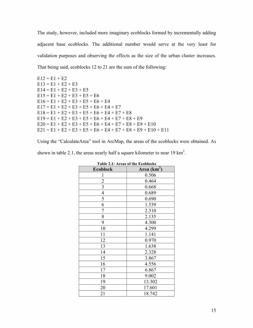
The study, however, included more imaginary ecoblocks formed by incrementally adding

adjacent base ecoblocks. The additional number would serve at the very least for

validation purposes and observing the effects as the size of the urban cluster increases.

That being said, ecoblocks 12 to 21 are the sum of the following:

E12 = E1 + E2 E13 = E1 + E2 + E3 E14 = E1 + E2 + E3 + E5 E15 = E1 + E2 + E3 + E5 + E6 E16 = E1 + E2 + E3 + E5 + E6 + E4 E17 = E1 + E2 + E3 + E5 + E6 + E4 + E7 E18 = E1 + E2 + E3 + E5 + E6 + E4 + E7 + E8 E19 = E1 + E2 + E3 + E5 + E6 + E4 + E7 + E8 + E9 E20 = E1 + E2 + E3 + E5 + E6 + E4 + E7 + E8 + E9 + E10 E21 = E1 + E2 + E3 + E5 + E6 + E4 + E7 + E8 + E9 + E10 + E11

Using the “CalculateArea” tool in ArcMap, the areas of the ecoblocks were obtained. As

shown in table 2.1, the areas nearly half a square kilometer to near 19 km2.

Table 2.1: Areas of the Ecoblocks Ecoblock Area (km2)

1 0.506 2 0.464 3 0.668 4 0.689 5 0.690 6 1.539 7 2.310 8 2.135 9 4.300 10 4.299 11 1.141 12 0.970 13 1.638 14 2.328 15 3.867 16 4.556 17 6.867 18 9.002 19 13.302 20 17.601 21 18.742

16

The population count for each ecoblock is as well an important defining characteristic,

and a parameter at the center of the computations to follow regarding water supply. In

order to obtain an estimate the census bureau data on MassGIS was used. Shapefiles of

census tracts based on the 2000 census data were downloaded. The shapefiles had

population attributes but a population density attribute was added and computed for all

tracts prior to clipping them to the boundary of each ecoblock. Since attributes that are

not maintained by ArcMap are retained as constant with any manipulation of the data

layer, retaining the population density and not the population is the accurate way if the

layer is to be clipped or joined. Then, the census tracts were clipped using each cluster

and the population of the ecoblock was calculated as the summation of the area of each

interior census tract multiplied by its population density.

Table 2.2: Population Estimates of the Ecoblocks Ecoblock Population Population Density

(persons/km2) 1 4,280 8,460 2 3,340 7,180 3 4,970 7,400 4 13,530 19,630 5 6,040 8,760 6 5,910 3,840 7 23,350 10,110 8 20,030 9,380 9 4,840 1,130 10 31,320 7,290 11 2,000 1,760 12 7,620 7,850 13 12,580 7,680 14 18,630 8,000 15 24,540 6,350 16 38,070 8,360 17 61,420 8,940 18 81,450 9,050 19 86,290 6,490 20 117,600 6,680 21 119,610 6,380

17

The population estimates are shown above in table 2.2 along with the overall population

densities for each ecoblock. At this point, it can be figured out from tables 2.1 and 2.2

that the clusters range in size from small community-like clusters to large urban hubs.

Another important consideration that should be discussed at this point is the land use in

each ecoblock which - as it will show later - will also affect water conservation. The 1999

land use dataset on MassGIS was as such downloaded and used to determine the land use

breakdown for the ecoblocks. A description of the land use code definitions is provided

in appendix B. For the interest of this study, residential, commercial, industrial, open

urban and transportation uses will be aggregated and tabulated. Table 2.3 shows the

codes used for the land uses of interest.

Table 2:3: Aggregated Codes for each Land Use Category

Land Use Category Aggregated Codes* Residential 10, 11, 12, 13 Commercial 15

Industrial 16 Transportation 18 Open Urban 3, 4, 7, 17

*Description of all codes is provided in Appendix B

Downloading the land use data layer from MassGIS and using the “Tabulate Areas”

functionality in ArcToolbox, with the tabulation parameter as the land use code, yields

measured surface areas for each land use code from which the percent for each category

can be calculated in each ecoblock. This procedure applies to the base ecoblocks while

for the others the percentages were calculated by weighted averages of their components.

Table 2.4 summarizes the results of the land use categorization and reveals that land use

18

is somewhat variable between ecoblocks. Residential, commercial and open urban classes

are the most predominant as it would be expected for typical urban areas.

Table 2.4: Land Use Composition of the Ecoblocks

Ecoblock %Residential %Commercial %Industrial %Open Urban

%Transportation

1 11 14 0 53 22 2 36 13 11 30 10 3 40 12 8 25 15 4 37 37 0 26 1 5 43 20 0 32 5 6 4 44 28 7 17 7 36 49 0 12 3 8 41 29 0 19 11 9 0 10 17 40 34 10 13 50 0 17 20 11 6 30 1 3 60 12 23 14 5 42 16 13 30 13 6 35 16 14 34 15 5 33 13 15 22 27 14 23 14 16 24 28 12 24 12 17 28 35 8 20 9 18 31 34 6 19 10 19 21 26 9 27 17 20 19 32 7 24 18 21 18 32 7 22 21

Figure 2.3 is a land use map of the area engulfing the ecoblocks which was used to obtain

the land use breakdown inside each cluster.

This area also suffers from subsidence in the pile foundations under many historic

buildings in the Back Bay area because of the lack of groundwater recharge and the drop

in the groundwater table despite the annual precipitation averaging 45 inches (NOAA,

2008). GHG emissions and below the nationwide average for the United States: 0.466

Tons CO2, 0.02647 Tons CH4 and 0.00616 Tons per MWh of electricity (DOE EIA,

2007).

19

±

0 2,000 4,0001,000 Meters

Projection: Lambert Conformal ConicCoordinate System: NAD 1983 Stateplane MA Mainland

Land Use Catgory

Crop Land

Pasture

Forest

Non-Forested Wetland

Mining

Open Land

Participation Recreation

Spectator Recreation

Water-Based Recreation

Multi-Family Residential

High Density Residential

Medium Density Residential

Low Density Residential

Salt Water Wetland

Commercial

Industrial

Urban Open

Transportation

Waste Disposal

Water

Woody Perennial

Land Use in South Boston

Figure 2.3: Land Use in South Boston

20

CHAPTER 3

WATER AND ENERGY CONSERVATION

The conservation of water, its reuse and source reduction are an integral part of

sustainable water management and an important component of integrated resource

management (Aquatex, 2008). With efficient water management at the building level

being an integral part of this study, this chapter enumerates the water and energy

conserving household practices that, if used in the household within the ecoblocks, would

generate savings in water supply and wastewater treatment as well as reduce the stress on

the regional waterbodies. Based on the New York City census figures, the per capita use

of water in 2003 was 136.6 gallons per day for all uses, down from 141.8 gallons in 2002

and 154.5 gallons in 2001. This decline can be associated with an awareness of the need

to conserve water, even in the Northeast of the US, as well as a way to plug the leaks in

the pipeline system.

3.1- Water Conservation

Conservation can de defined as any action that reduces water use, with the resources used

to generate the savings having a lesser value than the resources saved (DeMonsabert,

1998). The resources saved, in addition to water, can be fuel oil, natural gas and other

energy sources. Wilson (2008) stipulated that savings in water are necessarily tantamount

to savings in energy because of the “water-energy nexus”. For example, it is generally

assumed that wastewater treatment and pumping consumes 2.85 kWh per kgal treated.

Water conservation is achieved through low-flow fixtures and enhancement devices such

as automatic controls. Obviously the applicability of these devices depends on the use of

21

the structure and subsequently land use but their application is mandated by the Energy

Policy Acts of 1992 and 2005. The 1992 act introduced new water efficiency standards

which were aimed at significantly reducing the amount of water consumed by typical

fixtures: water closets, lavatory faucets, kitchen faucets, shower heads and others. Shortly

after it was enacted, a series of incentive programs were launched in multiple cities to

replace heavy usage fixtures with more efficient fixtures compliant with the Energy

Policy Act. In 1994, the New York City residential rebate program replaced 1,635,000

old-style water closets with units using 1.6 gallons per flush while the state of

Massachusetts also followed suit and ensured that only 1.6 gallons per flush toilets are

sold (MWRA, 2006).

However, for a sustainable use of water resources, according to DeMonsabert, water

conservation needs to be taken beyond the provisions of the Energy Policy Act as

technology has taken significant strides since 1992 and efficient water management

became a more persistent need. DeMonsabert (1998) proposed that efficiency be

evaluated on an individual basis for each target structure (commercial building,

residential, industrial, federal building) in a detailed and comprehensive assessment of

what fixtures can be optimized in a model he called the “Watergy” model. Watergy,

which combines water and indirect energy conservation, was used by DeMonsabert in a

study for the federal government to optimize water consumption in federal facilities. The

rationale behind the Watergy model is used this study on a more generalized scale to

optimize the water supply for each ecoblock. Subsequently the following is a listing of

the applicable water conserving fixtures as well as their contribution to savings in water

and energy.

22

3.1.1- Toilets and urinals

Toilets are among the best candidates for cost effective water consumption reduction,

representing about 35% of residential water use and up to 70% of interior water use in an

office building or commercial establishment (Metcalf and Eddy, 2003). Prior to 1994,

most toilets used 3.5, 5.5 or even up to 7 gallons per flush (gpf) but after the Energy

Policy Act, virtually most households were since equipped with 1.6 gpf in compliance

with the code. However, sustainability requires further refinement and suggests that ultra

low-flow water closets with 0.8 gpf be used in new developments. These toilets

according to Chanan at el. (2003) cost nearly the same as their code required

counterparts. With a difference of 0.8 gpf between the code required and the high

efficiency toilets, and using a typical number of 4 flushes/capita/day, savings equaling

3.2 gal/capita/day can be achieved in both residential and commercial buildings.

As for urinals, their use is restricted to commercial and some industrial establishments.

High efficiency waterless urinals are now available. Most of these systems operate

through the use of an oil barrier between urine and the surrounding air space thus

preventing odors from escaping. Waterless urinals would generate savings of 4

gal/male/day or 2 gal/capita/day.

3.1.2- Faucets and taps

Typical non-efficient taps usually use 2.5 gpm (gallons per minute) of flow. There’s

widespread use of automatic faucets incorporating infrared motion sensors and having the

potential to reduce the faucet’s flow by 70%. However, these fixtures would be too costly

for residences and small office buildings and their use is restricted to large structures such

as airports and shopping malls. Since the scope of this study is to research fixtures with a

23

base cost identical or close to the status quo fixtures, these automatic faucets are

excluded. Instead, a more efficient approach proposed by Chanan et el (2003), would be

adjusting the flow rate of taps while maintaining spray pattern through the installation of

flow regulating tap aerators. Such efficient taps would have a flow of 0.7 – 1.8 gpm.

Assuming a reduction to only 1.8 gpm – which happens at a minimal additional cost – 0.7

gpm can be saved relative to 2.5 gpm. Considering a use of 5 minutes per day for each

individual, at least 3.5 gal/capita/day of water savings can be achieved in both residential

and commercial buildings.

3.1.3- Showerheads

While showering may be the largest source of residential water demand, shower demand

is not as high in commercial buildings except for hotels. Typical non-efficient

showerheads have a flow rate of approximately 10 L/min (2.6 gpm) while the Energy

Protection Act requires the use of 2.5 gpm heads. Highly efficient showerheads only use

1.8 gpm (DeMonsabert, 1998) and the resulting savings of 0.7 gpm translate into 10.5

gal/capita/day with daily 15 minute showers per person.

3.1.4- Dishwashers and Washing Machines

After toilets and showerheads, washing machines make up the next largest percentage of

residential water use. Savings in this section will be quoted straight out of the “Watergy”

model where DeMonsabert reported that efficient washing machines yield savings of 4

gal/capita/day (55 gal per load - standard vs 42 gal per load - efficient at 0.2 loads per day

per person) while efficient dishwashers only yield savings of 1 gal/capita/day (14 gallons

per load - standard vs 8.5 gallons per load – efficient at 0.17 loads per person per day).

24

Therefore, from a water conservation perspective, this study will only assume the use of

efficient washing machines.

Putting it all together, tables 3.1 and 3.2 summarize the savings in the sections above for

residential and commercial buildings. The total savings will be applied to the proposed

water supply policy.

Table 3.1: Feasible Water Savings in Residential Households

Fixture/Machine Standard/Code Sustainable/Low-flow

Water Savings (gal/capita/day)

Water Closet 1.6 gpf 0.8 gpf 3.2

Faucets/Taps 2.5 gpm 1.8 gpm 3.5

Showerheads 2.5 gpm 1.8 gpm 10.5

Washing Machines 55 gal per load 42 gal per load 4

Total Water Savings 21.2

Table 3.2: Feasible Water Savings in Commercial Buildings

Fixture/Machine Standard/Code Sustainable/Low-flow

Water Savings (gal/capita/day)

Water Closet 1.6 gpf 0.8 gpf 3.2

Urinals 1 gpf 0 gpf 2

Showerheads 2.5 gpm 1.8 gpm 2.2*

Faucets/Taps 2.5 gpm 1.8 gpm 3.5

Washing Machines 55 gal per load 42 gal per load 1*

Total Water Savings 11.9

* Limited to hotels which are estimated to be 20% of commercial buildings in South Boston

The tables above show that 21.2 and 11.9 gallons/capita/day of fresh water can be saved

in residential and commercial buildings respectively. The more conservative and better

25

rounded figures of 20 and 10 gallons/capita/day will be used in subsequent analysis. A

reduction of 8 gallons/capita/day will also be used for industrial buildings.

The calculation of the yearly water savings for each ecoblock due to water conservation

(WSC) will be done by multiplying the total population by the percents of residential and

commercial/industrial land uses and then by the appropriate feasible water saving

computed above. This is represented by equation 3.1 and the results are tabulated in table

3.3.

WSC = Population ×(%Res×20 + %Com×10 + %Ind×8)×365 (3.1)

Table 3.3: Water Saved by Conservation Ecoblock WSC (m3/yr)

1 21,290 2 43,220 3 67,510 4 207,530 5 88,500 6 60,708 7 390,310 8 307,110 9 15,780 10 328,800 11 11,840 12 67,340 13 135,240 14 223,860 15 278,660 16 450,220 17 826,470 18 1,134,220 19 896,450 20 1,228,290 21 1,216,160

3.2- Energy Conservation

As briefly indicated in 3.1, energy can be saved indirectly by saving water and directly by

energy efficient appliances.

26

3.2.1- Indirect Energy Savings

When water is saved at the building level energy is saved in pumping and distribution,

water treatment, sewerage and wastewater treatment. Also, it has to be noted that the

quantity of water saved at the end user does not equal the water saved from a water

supply perspective due to unaccounted for (UAF) losses such as line leaks, breaks and

inefficient metering. The average water utility in Massachusetts has a 10% UAF factor

(AWWA, 1992). Leakage or UAF do not typically apply to wastewater systems since

wastewater collection is not usually pressurized. On the contrary, the problem is actually

infiltration and inflow into the waste flow. However, the assumption that every volume of

water conserved yields the same volume of wastewater reduction still holds. Appendix C

includes data regarding the energy requirements for water conveyance and treatments

obtained from the American Water Works Association (AWWA)’s Water Industry

Database (WIDB) as well as a presentation by Michael Wilson, CH2M HILL (NEWEA

Annual Conference 2008). Extracted from appendix C, the following numbers in table

3.4 will be used.

Table 3.4: Energy Requirement for Water-Related Works

Activity Energy Requirement (kWh/MG)

Water Supply and treatment 1800

Pumping and Distribution 700

Wastewater Collection and Treatment* 2000

* Treatment up to the Secondary Level

Using the figures above, the indirect energy savings (IES) in kWh per year can be

computed by equation 3.2.

IES = WSC ×(1800/0.9 + 700 + 2000) = 4700 ×WSC (3.2)

27

Using equation 3.2, the indirect energy savings can be computed for the ecoblocks in

study. The results are tabulated in table 3.5.

Table 3.5: Indirect Energy Savings

Ecoblock IES (kWh/yr) 1 26,440 2 53,670 3 83,830 4 257,700 5 109,890 6 75,380 7 484,660 8 381,350 9 19,600 10 408,280 11 14,700 12 83,620 13 167,930 14 277,980 15 346,020 16 559,050 17 1,026,260 18 1,408,400 19 1,113,160 20 1,525,220 21 1,510,160

3.2.2- Direct Energy Savings Direct savings are defined as savings to the end user and the supplier in the form of

reduced energy usage. Direct energy savings (DES) can be achieved by the reduction of

hot water use (already achieved by water conservation), the use of energy-efficient home

appliances and compact florescent lights. There are also significant direct energy savings

from green roofs but that will discussed in the relevant chapter.

Retracting to section 3.1, many water conserving fixtures were examined. Nonetheless,

only faucets, showerheads, dishwashers and washing machines use hot water and as such

28

are capable of generating direct energy savings. These savings depend on the efficiency

of the boiler and are not as important as the other components of DES. For that reason,

the numbers used by DeMonsabert in the “Watergy” model will be also used in this study

(table 3.6).

Table 3.6: Direct Energy Saving for Water Conserving Fixtures and Machines (DeMonsabert, 1998)

Fixture or Machine DES (kWh/capita/day)

Faucets 1

Showerheads 1

Washing Machines and Dishwashers 0.3

Outside the circle of water lies another key factor in sustainable development and

particularly energy conservation: electricity. In 2003, electricity used in housing units

accounted for 22% of the US energy consumption (Hojjati and Battles, 2005). Also

according to the 1997 Residential Energy Consumption Survey, lighting and appliances

used 27% of household electricity and accounted for more than 45% of the energy costs.

Realizing the need to reduce the toll of high electrical consumption, the US EPA, in

conjunction with the Department of Energy launched the Energy Star program which

identifies high efficiency appliances and rates the models that exceed the federal

minimum efficiency standard (by 15-20%). The Energy Star program calculated that at

least 300 kWh of energy (per household) can be saved annually by using appliances

labeled with an Energy Star tag. Much more significant savings can be accrued in

specific cases and households. There are even high performance appliances that yield

great savings in energy over their life cycle but with a relatively large initial cost. For the

scope of this study, the simple savings of 300 kWh per household or 75 kWh per capita

29

(based on an average occupancy of 4 persons per housing unit) will be used. Energy Star

still estimates that, despite fairly widespread use, half of the appliances nationwide are

not rated. As such, it will be assumed that for optimal energy performance, households in

the ecoblocks would conserve 150 kWh per unit.

More direct energy savings however can be achieved through CFLs (Compact

Fluorescent Lamps). Standard pear-shaped incandescent lamps produce a lot of heat,

which prompted the Energy Star program to recommend the use of CFLs to save energy

and money while still providing quality light especially in high use lighting areas such as

kitchens, living rooms and outdoor fixtures. EPA also reassures consumers that CFLs

safely produce steady, quiet and warm light while the problems of poor color and little

noise that plagued the first generations of these lights have been eliminated. They also

come in a variety of shapes and sizes to fit different fixtures. The main advantage though

is that they use far less watts than incandescent lights in order to produce the same light.

As shown in table 3.7, CFLs consume at least 25% of watts used by incandescent lights

but they still produce the same light intensity measured in Lumens. However, even

though CFLs are recommended by Energy Star, only 1.5 out of 43 household in Boston

use any sort of CFL according to a survey conducted at the energy efficiency department

at NSTAR, a major power supplier for Boston residences (2006).

Table 3.7: Equivalent Wattage for CFLs for the Same Light Output (Source: EnergyStar.com)

Incandescent Bulb Compact Fluorescent Light Output (Lumens) 40 W 13 W 490-510 60 W 15 W 870-890 75 W 20 W 1190-1200 100 W 25 W 1680-1705

30

Therefore, considerable savings in energy can be achieved by using CFLs in the

theoretical ecoblocks of this study. Using a typical wattage requirement of 1.5 W/ft2, an

average daily usage of 5 hours, the building footprints area with a minimum of 3 stories,

and a reduction factor of 0.4, the savings by using CFLs were computed. The results are

shown in table 3.8.

Table 3.8: Energy Savings Provided by CFLs Ecoblock Energy Savings (MWh/yr)

1 3866.2 2 2515.3 3 6793.6 4 7062.9 5 3354.4 6 9469.3 7 18350.9 8 17966.3 9 17445.4 10 33211.9 11 5942.7 12 6381.4 13 13175.0 14 20237.9 15 23592.2 16 33061.6 17 51412.4 18 69147.3 19 86592.7 20 119804.6 21 125747.3

31

CHAPTER 4

VEGETATED ROOFS

Green roofs or vegetated roofs use engineered growing media, drought tolerant plants,

and specialized roofing materials installed on existing structures (Peck et al., 1999). This

makes the rooftop capable of absorbing and retaining stormwater rather then rapidly

conveying it into stormwater drainage systems. Therefore, they are a kind of structural

controls designed to treat stormwater and mitigate the effects of increased runoff peak

rate and volume due to urbanization. Variants of vegetated roofs have been used

throughout history, but modern designs were mostly developed in Germany in the 1960s.

As such, green roofs have traditionally been mostly used in Europe (and in Scandinavia

for centuries) but they are becoming increasingly popular in North America. As this study

is not centered on green roofs, the chapter will deal with this topic strictly from a

sustainability perspective.

4.1- Implementation of Green Roofs in this Study

One component of the NPDES permitting process is the requirement to use stormwater

BMPs (Best Management Practices). Most common BMPs such as stormwater ponds,

wetlands, and vegetated swales are used to meet the goals of water quality enhancement

and flood protection but their major drawback is their land requirement. Readily available

undeveloped space is scant in urbanized and metropolitan areas meaning that it would

probably be easier for stormwater management to be implemented within or into the built

environment. Remarkably, according to Carter (2007) rooftops have been overlooked as a

tool for solving urban environmental problems even though they constitute a large

32

fraction of the total impervious surface cover (ISC). Moreover, studying the application

of green roofs within the frame of watershed management is more of a clear-cut relative

to other practices such as rain gardens or pervious pavement because the matrix of their

application (i.e. the concrete roof) can be easily identified and loaded into tools such as

GIS. Virtually all cities in the US have developed GIS layers of their building footprints

and that is greatly propitious for the study of green roofs. On the other hand for instance,

the study of rain gardens or pervious pavements is parcel-specific because of the complex

factors governing their application (e.g. location of catch basins, traffic loads …) and it

would be rather hard to find a tool that helps the study of their application on a watershed

basis.

The main concern for retrofitting green roofs on existing structure is the risk of exceeding

its load bearing capacity. However, this concern will not be touched upon in this study

firstly because it involves the use of an extensive (rather thin) type of vegetated roof

which is not expected to put much strain on the structure and secondly because the life

cycle assessment will be done for imaginary ecoblocks assumed to be developed from

scratch where the use of vegetated roofs has been accounted for.

In this research project, stormwater retention, the mitigation of peak flows and the

thermal insulation effects of green roofs will be quantified. Eventually, the calculation of

the total Direct Energy Savings (DES) will be possible at the end of this chapter. Data in

this study regarding the hydrologic behavior of green roofs rely heavily on research being

conducted at the Institute of Ecology in the University of Georgia, Athens, GA under the

supervision of Dr. Timothy Carter. A 42.64 m2 and about 3-in thick simple to build and

easy to replicate green roof test plot was established on the campus using an American

33

Hydrotech – a supplier for the specialized green roofing materials – extensive roof

garden. Supplied materials included “a WSF40 root protection sheet, an SSM45 moisture

retention mat, a floradrain FD04 synthetic drainage panel, and a Systenfilter SF geotextile

filter sheet”2 (American Hydrotech, 2002). The growing media was a lightweight roof

garden mix provided by ItSaul Natural while the soil mix was a blend of 55% stalite

expanded slate, 30% USGA sand and 15% organic matter. Also, six drought-tolerant

species of plantation were chosen because of their ability to survive heat, temperature

fluctuation, and low moisture and nutrient conditions at the roof surface. A photo of the

test plot at the University of Georgia, as well as a cross section of the researched green

roof adapted in this study, are shown in figure 4.1.

Figure 4.1: Green Roof Tested at the University of Virginia (Carter and Keeler, 2007)

2 quoted from Carter and Keeler (2007)

34

The matrix of application of the above extensive green roof is the rooftops of the

buildings within the ecoblocks which is generally equal to the building footprint area

(BFA). The rooftop is typically the same size as the building’s footprint and is the

structure’s barrier against rainfall and solar radiation. As indicated earlier, it has been

overlooked as a space with the potential to become an environmental amenity rather than

an impervious surface contributing to urban runoff. To the extent that this is possible, the

whole building becomes “economically and functionally more efficient with a more

benign effect on the surrounding landscape” (Carter and Keeler, 2007). Hence, a GIS

layer of the building footprints in the metropolitan Boston area was downloaded from

MassGIS and clipped to the boundaries of the ecoblocks one at a time, in order to obtain

building footprints datasets for each one of them. Figure 4.2 is a map showing the

building footprints in the ecoblocks with a zoom on ecoblock 1 where the building

footprints were filled with a roof garden pattern. It should also be noted that since

clustering was done based on major roads, no footprint is cut or distorted.

Using the functionalities of ArcMap, the total BFA was calculated for each cluster by

summing the individual areas of the footprints inside the ecoblock, a field that is

automatically maintained by ArcMap. For practical purposes, it will be assumed that the

above described green roof will be retrofitted on 70% of the rooftop area (or BFA) to

account for some cases of inadequacy or presence of roof equipments. The green roofs

area (GRA) will as such be the measured BFA multiplied by 0.7. The BFA and GRA for

the ecoblocks are tabulated in table 4.1 and constitute important parameters for the

calculations to follow (water retention, peak flow reduction and energy conservation by

green roofs).

35

1 1

1 0

98

7

6

5

4

3

2

±

0 1,800 3,600900 MetersProjection: Lambert Conformal ConicCoordinate System: NAD 1983 Stateplane MA Mainland

Building Footprints in the Ecoblocks

A Zoom on Ecoblock 1

Figure 4.2: Building Footprints with a Zoom on Ecoblock 1

36

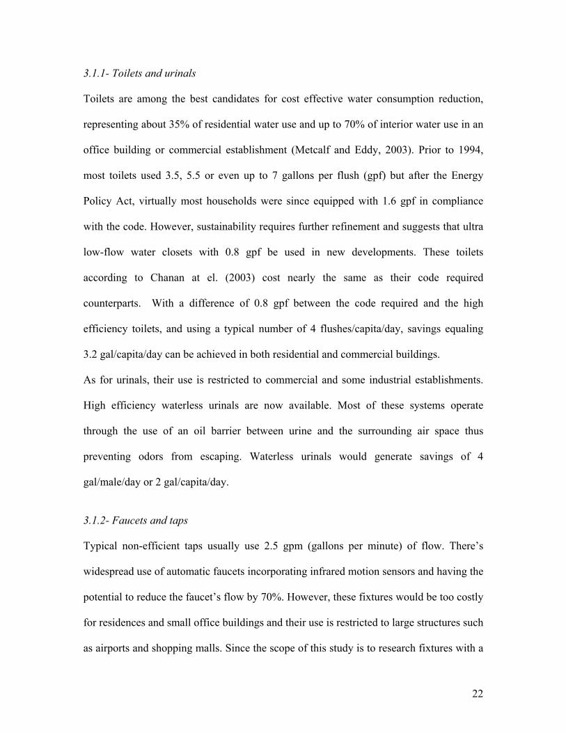
Table 4.1: BFA and GRA of Ecoblocks Ecoblock BFA (m2) GRA (m2)

1 150,308 105,216 2 97,789 68,452 3 264,119 184,883 4 274,590 192,213 5 130,411 91,288 6 368,148 257,704 7 713,443 499,410 8 698,493 488,945 9 678,242 474,769 10 1,291,209 903,846 11 231,038 161,727 12 248,097 173,668 13 512,216 358,551 14 786,806 550,764 15 917,217 642,052 16 1,285,365 899,756 17 1,998,808 1,399,166 18 2,688,301 1,881,811 19 3,366,543 2,356,580 20 4,657,752 3,260,426 21 4,888,790 3,422,153

4.2- Water Retention by Green Roofs

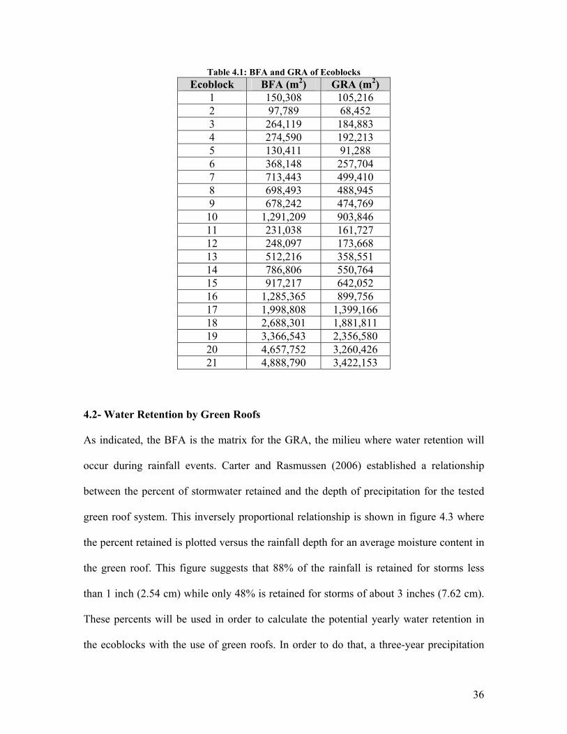
As indicated, the BFA is the matrix for the GRA, the milieu where water retention will

occur during rainfall events. Carter and Rasmussen (2006) established a relationship

between the percent of stormwater retained and the depth of precipitation for the tested

green roof system. This inversely proportional relationship is shown in figure 4.3 where

the percent retained is plotted versus the rainfall depth for an average moisture content in

the green roof. This figure suggests that 88% of the rainfall is retained for storms less

than 1 inch (2.54 cm) while only 48% is retained for storms of about 3 inches (7.62 cm).

These percents will be used in order to calculate the potential yearly water retention in

the ecoblocks with the use of green roofs. In order to do that, a three-year precipitation

37

series for Boston was obtained from the National Oceanic and Atmospheric

Administration (NOAA)’s database. The precipitation, spanning from 01/01/2005 to

12/31/2007, is provided in appendix D along with the amount of rainfall retained from

each daily amount of precipitation. Care was taken in observing and analyzing the rainfall

data so that these computations were applied to intermittent moderate storms that

maintain a low to average moisture content in the vegetated roof.

Figure 4.3: Retention Percentages for Different Categories of Rainfall (Carter and Rasmussen, 2006)

The results of the computation provided in appendix D are summarized in table 4.2. The

average retention is 75% of the yearly rainfall or 83.45 cm will be used to calculate the

volume of annual retention.

Table 4.2: Water Retention Computations

Year 2005 2006 2007

Total Rainfall (cm) 108.79 129.59 96.24 Depth Retained by Green roofs (cm) 84.45 94.64 71.27

% Retention 78 73 74

38

The volume (in m3) of water retained yearly by the green roofs (YWR) will be calculated

for each ecoblock by multiplying the GRA inside the ecoblock by the average retention

depth for Boston per year. This retained water, which could otherwise end up being

discharged into combined sewers, in turn brings about indirect savings in energy similar

to water conservation. The amounts are tabulated below in table 4.3.

Table 4.3: Yearly Water Retention by Green Roofs

along with Indirect Energy Savings Ecoblock YWR (m3/yr) IESGR (kWh/year)*

1 87,800 46,390 2 57,120 30,180 3 154,290 81,530 4 160,400 84,760 5 76,180 40,250 6 215,050 113,630 7 416,760 220,220 8 408,030 215,600 9 396,200 209,350 10 754,260 398,550 11 134,960 71,310 12 144,930 76,580 13 299,210 158,100 14 459,610 242,860 15 535,790 283,110 16 750,850 396,750 17 1,167,600 616,960 18 1,570,370 829,780 19 1,966,570 1,039,104 20 2,720,830 1,437,690 21 2,855,790 1,509,000

* based on 2000 kWh/MG for Wastewater Collection and Treatment (Wilson, 2008)

4.3- Peak Flow and Runoff Reduction by Green Roofs

The reduction in peak flows and urban runoff will be computed using the NRCS-CN

(National Resources Conservation Service – Curve Number) model which is widely used

amongst engineers and watershed analysts. Residential, commercial and industrial areas

39

were assigned CNs of 92, 92 and 88 respectively while impervious surfaces such as

transportation related surfaces were assigned a CN of 98 and a CN of 67 was used for

open urban spaces (NRCS, 1986). Composite CNs representing the status-quo (traditional

roofs) were determined for the ecoblocks by calculating averages weighted by the land

use classifications. Carter and Rasmussen (2006) experimentally derived a CN of 86 for

green roofs by regressing storage and runoff. This CN was assigned to 70% of the

residential and commercial areas in the ecoblocks and new composite CNs representing

the scenario with green roofs were computed. The CNs for the ecoblocks with traditional

roofs (TR) and green roofs (GR) are shown in table 4.4. The calculations in this section

were performed for the base ecoblocks along with ecoblock 21 (all ecoblocks).

Table 4.4: Curve Numbers with Traditional and Green Roofs

Ecoblock CNTR CNGR 1 80.6 79.4 2 84.3 82.2 3 86.3 84.1 4 85.3 82 5 84 81.6 6 89.1 86.4 7 88.7 84.7 8 87.4 84.4 9 83.8 82.9 10 88.7 85.3 11 94.3 92.3 21 86.8 84.2

Runoff modeling was performed using Hydraflow-Hydrographs 2007 using the

composite CNs above for the two scenarios of traditional and green roofs. The chosen

storms for the analysis were the 1, 10 and 50-year storms to understand how the results

vary with the storm frequency. Using normalized storm duration-frequency-intensity

curves (Novotny et al., 1989), the 1, 10 and 50-year 6-hour precipitation values for

40

Boston were calculated as 36 mm (1.42 in), 72 mm (2.83 in) and 156 mm (6.14 in)

respectively. In the Hydraflow model, an average basin slope of 0.4% and a hydraulic

length of 100ft were used as typical values for urban areas. The peak flows, runoff depths

as well as the reductions with the use of green roofs are shown below in tables 4.5 and

4.6.

Table 4.5: Peak Flow Differences in the Ecoblocks between Traditional and Green Roofs

P 1 = 1.42” (36 mm) P 10 = 2.83” (72 mm) P50 = 6.14” (156 mm)

Ecoblock Qp TR Qp GR % Red Qp TR Qp GR % Red Qp TR Qp GR % Red

1 0.655 0.544 17 3.52 3.27 7.1 12.46 12 3.7 2 0.973 0.775 20 4 3.6 10 12.52 12 4.3 3 1.1 0.825 25 4.8 4.3 9.5 15.1 14.5 4 4 1.6 1.08 32.5 6.22 5.2 16.4 19 17.58 7.5 5 1.38 1.03 35 5.8 5.08 12.4 18.43 17.42 5.5 6 5.15 3.93 23.7 16.21 14.27 12 43.7 41.63 4.7 7 7.44 5 32.8 23.9 20.18 15.6 65.17 62.75 3.7 8 6.05 4.47 26 20.78 18.35 11.7 58.86 57.6 2.2 9 8.4 7.54 10.2 35.75 34 5 114.42 112 2.1 10 13.84 10 27.7 44.47 38.8 12.8 121.25 118.37 2.4 11 6.07 5.14 15.3 14.76 13.74 6.9 34.77 34 2.3 21 50 38.4 23.2 177.2 159.3 10.1 511 503.2 1.5

The results in the tables 4.5 and 4.6 give clear indications on the effect of widespread

roof greening on the hydrology of urban subwatersheds. This effect is dependent on two

factors: the Rooftop Cover (RTC) and the design storm. The RTC normalized by the area

of the ecoblock were the highest for ecoblocks 3, 4 and 14 (0.4, 0.4 and 0.34) and lowest

for ecoblocks 2, 5 and 9 (0.21, 0.19 and 0.16). The variety of RTCs and land uses in this

study help evaluate the efficiency of green roofs from a stormwater management

perspective under different scenarios.

41

Table 4.6: Runoff Differences in the Ecoblocks between Traditional and Green Roofs P 1 = 1.42” (36 mm) P 10 = 2.83” (72 mm) P50 = 6.14” (156 mm)

Ecoblock R TR R GR % Red R TR R GR % Red R TR R GR % Red

1 6.66 5.87 11.8 29.55 27.74 6.1 100.88 97.73 3.1 2 9.54 7.81 18.1 35.61 32.08 10.0 110.78 105.12 5.1 3 11.43 9.36 18.1 39.21 35.26 10.1 116.25 110.24 5.2 4 10.45 7.66 26.7 37.38 31.75 15.0 113.50 104.59 8.0 5 9.28 7.36 20.6 35.09 31.11 11.3 109.96 103.52 5.9 6 14.58 11.53 21.0 44.68 39.39 11.8 124.05 116.53 6.1 7 14.09 9.90 30.0 43.87 36.31 17.2 122.93 111.87 9.0 8 12.59 9.63 23.6 41.30 35.78 13.4 119.29 111.05 7.0 9 9.10 8.36 8.2 34.74 33.23 4.4 109.42 107.00 2.2 10 14.09 10.45 25.8 43.87 37.38 14.8 122.93 113.50 7.7 11 22.46 19.05 15.2 56.37 51.62 8.4 138.98 133.17 4.2 21 11.95 9.45 21.0 40.15 35.43 11.7 117.63 110.51 6.1

Reductions in surface runoff of 30% for the one-year storm, 17% for the ten-year storm

and 9% for the fifty-year storm were calculated in table 4.6 for ecoblock 7, a highly

urbanized ecoblock at the heart of South Boston. At the parcel level, the reduction in

runoff will tend to be much higher while it gets masked when ecoblocks are aggregated

into larger ones and properties become more uniform, as shown in table 4.6 where the

reductions level off and even decrease as the scale edges to a watershed level. When

green roofing is considered as a tool to minimize the impact of stormwater, areas zoned

commercial, industrial, institutional centers or sizeable residences which are known to

contain large flat-roofed buildings should be targeted. Ecoblock 7, which bears the best

results, has the highest commercial land use percentage (49%).

The second major factor governing the findings in this section is the design storm. As the

precipitation increases, runoff volumes increase and associated runoff reductions from

vegetated roofs are lessened. The drop in stormwater retention is the outcome of the roof

42

reaching its maximum saturation content and then quickly releasing rainfall from large

storms similar to a conventional concrete roof. Therefore, regardless of the scale of green

roof installation, the change in the hydrology of across a watershed will be minimal with

storm events larger than the one or two-year storm. Thus, it is important to consider the

rainfall distribution pattern for the specific watershed. Frequent storms of light rain will

be better retained by the vegetated roof than sporadic heavy downpours. In Boston, MA,

a large number of storms follow a pattern suitable for green roofing, hence the 75%

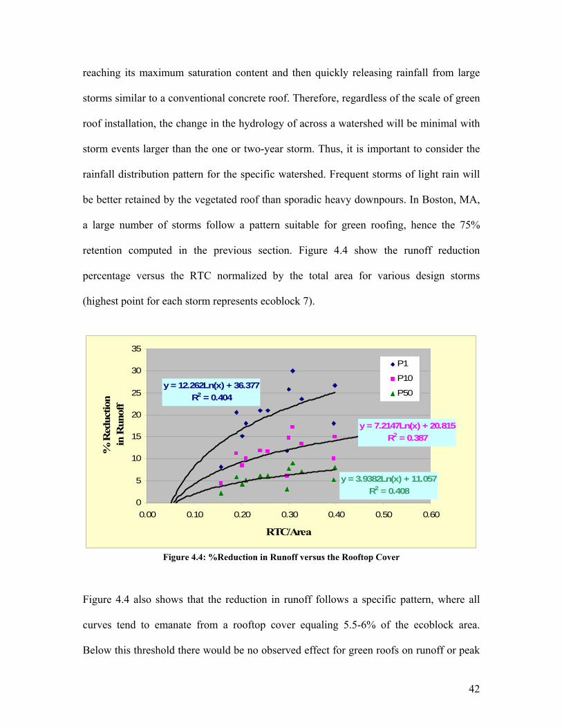
retention computed in the previous section. Figure 4.4 show the runoff reduction

percentage versus the RTC normalized by the total area for various design storms

(highest point for each storm represents ecoblock 7).

y = 12.262Ln(x) + 36.377R2 = 0.404

y = 7.2147Ln(x) + 20.815R2 = 0.387

y = 3.9382Ln(x) + 11.057R2 = 0.408

0

5

10

15

20

25

30

35

0.00 0.10 0.20 0.30 0.40 0.50 0.60

RTC/Area

% R

educ

tion

in R

unof

f

P1

P10

P50

Figure 4.4: %Reduction in Runoff versus the Rooftop Cover

Figure 4.4 also shows that the reduction in runoff follows a specific pattern, where all

curves tend to emanate from a rooftop cover equaling 5.5-6% of the ecoblock area.

Below this threshold there would be no observed effect for green roofs on runoff or peak

43

flows. As such, green roofs would not produce any reductions in runoffs or peak flows in

areas with sparse buildings like rural areas. Additionally, Novotny (2003) noted that the

CSO initiating rainfall intensity for typical US conditions is about 1 mm/hr, which is far

less than the intensities of the considered designed storms: 6 mm/hr for the one-year

storm, 12 mm/hr for the ten-year storm and 26 mm/hr for the fifty-year storm. As such,

green roofs could eliminate many CSOs.

However, while green roofs produce some significant peak flow shaving and drop in

runoff volume (and probably eliminate many CSOs), it cannot be solely relied upon for

stormwater management in a subwatershed or urban area. The little reductions for large

storm events mean that there would hardy be any economic benefits through decreasing

the sizing of culverts and pipes which are designed for such large events. In order to

achieve better runoff reductions and economic savings, stormwater management policies

should coupled vegetated roofs with green walkways or rain gardens which will reduce

the impact of areas directly connected to the storm sewer system.

4.4- Direct Energy Savings with Green Roofs

A more economically relevant attribute of green roofs is energy and insulation. Vegetated

roofs act to reduce the temperature of the roof surface through leaf shading direct solar

radiation, evaporation of moisture content and transpiration of plants which cool the

ambient air above the roof. Research by Wong et al. (2003) suggests that significant

savings in energy can be reaped with the use of green roofs and that plays an important

role in life cycle assessments of green roofs.

Carter and Keeler (2007) reported an insulating value (R-value) for the tested green roof

equal to 2.8 K.m2/W and similar to an inch of fiberboard. The R-value, a measure of

44

thermal resistance, describes the effectiveness of a material as a thermal insulator while

the inverse of R, the U-value or the coefficient of thermal conductivity, describes the rate

at which heat flows through the material with no regard to the heat source. Carter derived

the R-value with a second experimental roof, automated in situ measurement of radiation

and temperature and building energy models. Cost savings from additional insulation

provided by green roofs and the drop in heating and cooling loads will be computed by

the fundamental heat transfer equation:

Q (in Watts) = U×A×ΔT or (1/R) ×A×ΔT (4.1)

where A is the area of green roofs inside the ecoblock (GRA) and ΔT is the temperature

difference between the outdoor and the indoor environments. An average ΔT of 12°C or

K (21°F) was computed for Boston by assuming an indoor temperature of 72°F and

averaging the deviations from the monthly average temperatures. This computation is

shown in table 4.7.

Table 4.7: Computation of Average ΔT

Month Average Temperature* (°F) ΔT**

January 29 43 February 31.5 40.5 March 38.5 33.5 April 48.5 23.5 May 58.5 13.5 June 68 4 July 73.5 1.5

August 72 0 September 65 7

October 54 18 November 45 27 December 35 37

Average ΔT 21°F or 12°C* Mean of average high and average low (NOAA, 2008)

** With respect to an indoor temperature of 72 °F

45

Table 4.8: Yearly Energy Savings Provided by Green Roofs Ecoblock Energy Savings (MWh/yr)

1 3,950 2 2,570 3 6,940 4 7,220 5 3,430 6 9,670 7 18,750 8 18,360 9 17,820 10 33,930 11 6,070 12 6,520 13 13,460 14 20,680 15 24,100 16 33,780 17 52,520 18 70,640 19 88,470 20 122,400 21 128,470

Having ΔT, GRA and R, the yearly energy savings by green roofs in kWh were computed

for the ecoblocks using equation 4.1 based on 8760 hours per year of heating/cooling and

the results tabulated in table 4.8. When a kWh is converted into its dollar equivalent, it

would be found that green roofs have a yearly energy savings of $6.76 /m2.

Q (in kWh) = GRA37.54 or kWh/m 5437K 12GRAW/kW 1000hr/yr 8760

/WK.m 821 2

2 ×=××× ..

Additional unquantified cooling is provided by green roofs during the summer, since the

retained water (computed in section 4.2) would evaporate and absorb heat in the process

(the latent heat of water – the amount of heat absorbed or released during a phase change

– is 2260 J/g or 540 calories/g).

46

A computation of the total DES (Direct Energy Savings) combining direct savings from

hot water conservation, energy conservation, CFLs and the above computed savings from

green roofs can now be done. The DES for the ecoblocks are shown below in table 4.9.

Table 4.9: Total Direct Energy Savings in Ecoblocks

Ecoblock DES (MWh/yr) 1 11,570 2 8,010 3 18,090 4 26,150 5 12,080 6 24,330 7 57,580 8 53,890 9 39,510 10 94,600 11 13,770 12 19,580 13 37,670 14 57,250 15 69,210 16 100,230 17 157,800 18 211,220 19 250,730 20 345,340 21 359,110

4.5- Cost Considerations

Carter reported a cost of $116.76/m2 for the tested green roof, a figure which would be

used to calculate the cost of green roofing within the different ecoblocks. However, since

this cost is pertinent only to Athens, GA where the roof was tested, a locational

adjustment factor is needed to render this cost usable in subsequent calculations. Such

factor was estimated from RS Means (2008) for materials and workmanship between

Atlanta, GA and Boston, MA to be 1.3. In other words, civil engineering works in Boston

47

cost 30% more than Atlanta. The final adjusted costs of green roofs are presented in table

4.10.

Table 4.10: Cost of Green Roofs Ecoblock Cost of Green Roofs ($)

1 15,970,530 2 10,390,190 3 28,063,020 4 29,175,630 5 13,856,420 6 39,116,370 7 75,804,450 8 74,215,980 9 72,064,240 10 137,192,980 11 24,548,220 12 26,360,720 13 54,423,740 14 83,599,370 15 97,455,790 16 136,572,160 17 212,376,610 18 285,636,330 19 357,700,570 20 494,893,540 21 519,441,760

48

CHAPTER 5

WATER SUPPLY, RECLAMATION AND REUSE

The water supply and wastewater treatment in the urban green clusters or ecoblocks

would follow the principles of water conservation for the supply and water reuse for the

treatment.

5.1- Water Supply

Massachusetts regulations (#8810) (Division of Water Supply, 1989) stipulate that water

supply systems should be designed for a residential indoor water use of 100 gallons per

capita per day. This number figures heavily in the literature and has been recommended

by as well by the American Water Works Association (AWWA, 1999) and Metcalf and

Eddy (2003). A typical breakdown of the 100 gallons per day is shown in table 5.1.

Table 5.1: Typical Distribution of Residential Water Use

(Metcalf and Eddy, 2003 and AWWA, 1999) Percent of Total

Use Range Typical Shower 12-20 16.8

Bath 1-3 1.7 Faucet 12-18 15.7

Dishwashing 1-2 1.4 Clothes Washing 12-28 21.8 Other Domestic 0-9 2.2 Toilet Flushing 23-31 26.7

Leakage 5-22 13.7 Total 100

However, if regulations are changed in order to account for water conservation, 20

gallons/cap/day - which can be conserved in residential buildings as demonstrated in

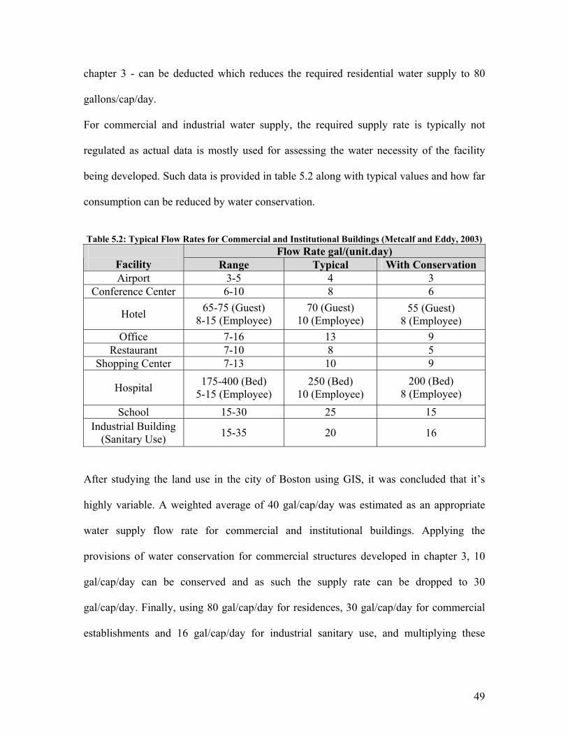
49

chapter 3 - can be deducted which reduces the required residential water supply to 80

gallons/cap/day.

For commercial and industrial water supply, the required supply rate is typically not

regulated as actual data is mostly used for assessing the water necessity of the facility

being developed. Such data is provided in table 5.2 along with typical values and how far

consumption can be reduced by water conservation.

Table 5.2: Typical Flow Rates for Commercial and Institutional Buildings (Metcalf and Eddy, 2003)

Flow Rate gal/(unit.day) Facility Range Typical With Conservation Airport 3-5 4 3

Conference Center 6-10 8 6

Hotel 65-75 (Guest) 8-15 (Employee)

70 (Guest) 10 (Employee)

55 (Guest) 8 (Employee)

Office 7-16 13 9 Restaurant 7-10 8 5

Shopping Center 7-13 10 9

Hospital 175-400 (Bed) 5-15 (Employee)

250 (Bed) 10 (Employee)

200 (Bed) 8 (Employee)

School 15-30 25 15 Industrial Building

(Sanitary Use) 15-35 20

16

After studying the land use in the city of Boston using GIS, it was concluded that it’s

highly variable. A weighted average of 40 gal/cap/day was estimated as an appropriate

water supply flow rate for commercial and institutional buildings. Applying the

provisions of water conservation for commercial structures developed in chapter 3, 10

gal/cap/day can be conserved and as such the supply rate can be dropped to 30

gal/cap/day. Finally, using 80 gal/cap/day for residences, 30 gal/cap/day for commercial

establishments and 16 gal/cap/day for industrial sanitary use, and multiplying these

50

figures by the land use percentages and the population of each ecoblock, the water supply

requirement for each ecoblock can be computed. The results are shown in table 5.3.

Table 5.3: Water Supply Flow Rate

Ecoblock Water Supply Rate (MGD) 1 0.223 2 0.182 3 0.295 4 0.744 5 0.388 6 0.128 7 1.195 8 1.187 9 0.054 10 1.263 11 0.075 12 0.410 13 0.716 14 1.093 15 1.001 16 1.642 17 2.847 18 4.015 19 3.791 20 5.029 21 5.037

5.2- Wastewater Treatment and Reuse

In green urban clusters, wastewater should be treated in order to have a high quality

effluent suitable for reuse. Wilson (2008) claimed that it takes around 6400 kWh per MG

(or $14 per MG) of energy to treat wastewater to acceptable levels of nitrogen and BOD

and any wastage of wastewater is wastage of energy. McCarty (2008) even went further

and called wastewater a resource.

One of the popular treatment processes to reclaim water for restricted uses is the

Biological Nutrients Removal process (BNR) (with filtration). Other technologies include

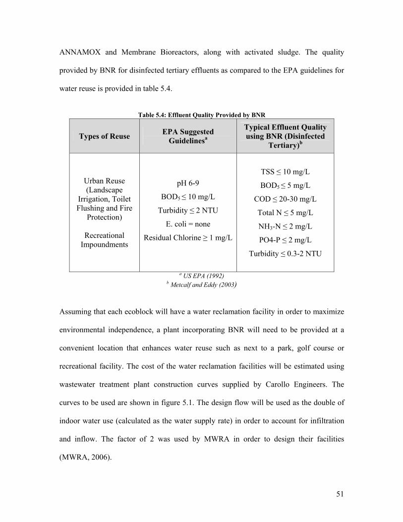
51

ANNAMOX and Membrane Bioreactors, along with activated sludge. The quality

provided by BNR for disinfected tertiary effluents as compared to the EPA guidelines for

water reuse is provided in table 5.4.

Table 5.4: Effluent Quality Provided by BNR

Types of Reuse EPA Suggested Guidelinesa

Typical Effluent Quality using BNR (Disinfected

Tertiary)b

Urban Reuse (Landscape

Irrigation, Toilet Flushing and Fire

Protection)

Recreational Impoundments

pH 6-9

BOD5 ≤ 10 mg/L

Turbidity ≤ 2 NTU

E. coli = none

Residual Chlorine ≥ 1 mg/L

TSS ≤ 10 mg/L

BOD5 ≤ 5 mg/L

COD ≤ 20-30 mg/L

Total N ≤ 5 mg/L

NH3-N ≤ 2 mg/L

PO4-P ≤ 2 mg/L

Turbidity ≤ 0.3-2 NTU

a US EPA (1992)

b Metcalf and Eddy (2003)

Assuming that each ecoblock will have a water reclamation facility in order to maximize

environmental independence, a plant incorporating BNR will need to be provided at a

convenient location that enhances water reuse such as next to a park, golf course or

recreational facility. The cost of the water reclamation facilities will be estimated using

wastewater treatment plant construction curves supplied by Carollo Engineers. The

curves to be used are shown in figure 5.1. The design flow will be used as the double of

indoor water use (calculated as the water supply rate) in order to account for infiltration

and inflow. The factor of 2 was used by MWRA in order to design their facilities

(MWRA, 2006).

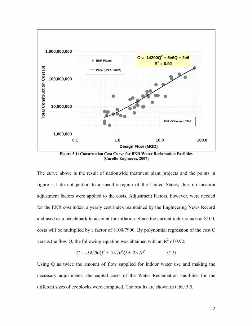
52

C = -14200Q2 + 5e6Q + 2e6R2 = 0.92

1,000,000

10,000,000

100,000,000

1,000,000,000

0.1 1.0 10.0 100.0Design Flow (MGD)

Tota

l Con

stru

ctio

n C

ost (

$)

BNR Plants

Poly. (BNR Plants)

ENR CCI Index = 7900

Figure 5.1: Construction Cost Curve for BNR Water Reclamation Facilities

(Carollo Engineers, 2007)

The curve above is the result of nationwide treatment plant projects and the points in

figure 5.1 do not pertain to a specific region of the United States; thus no location

adjustment factors were applied to the costs. Adjustment factors, however, were needed

for the ENR cost index, a yearly cost index maintained by the Engineering News Record

and used as a benchmark to account for inflation. Since the current index stands at 8100,

costs will be multiplied by a factor of 8100/7900. By polynomial regression of the cost C

versus the flow Q, the following equation was obtained with an R2 of 0.92:

C = -14200Q2 + 5×106Q + 2×106 (5.1)

Using Q as twice the amount of flow supplied for indoor water use and making the

necessary adjustments, the capital costs of the Water Reclamation Facilities for the

different sizes of ecoblocks were computed. The results are shown in table 5.5.

53

Additionally, a yearly cost for water management within the ecoblock should be

calculated to account for supply, distribution, pumping and treatment up the reuse

standards. As shown in table C.1 in appendix C, Wilson (2008) reported an energy

requirement of 10470 kWh per million gallons of water in order to supply water and then

reclaim it in a treatment facility in Massachusetts. The Energy Information

Administration also reported that a kWh of energy (electricity) in Boston costs $0.1938

and is sold to customers at $0.2017 (EIA, 2006). Using the figures above, yearly

operational costs to cover water supply and treatment in the ecoblocks were computed

and are also presented below in table 5.5.

Table 5.5: Capital Costs of Water Reclamation Facilities and Yearly

Ecoblock Capital Cost Of WRF ($)

Yearly Operational Cost (Supply and Treatment)

1 4,330,220 164,870 2 3,912,690 134,640 3 5,067,090 218,250 4 9,649,950 551,250 5 6,015,190 287,000 6 3,359,340 94,600 7 14,219,180 884,980 8 14,142,270 879,340 9 2,603,920 39,980 10 14,902,840 935,060 11 2,816,320 55,330 12 6,243,310 303,560 13 9,367,130 530,650 14 13,192,470 809,840 15 12,259,100 741,610 16 18,731,900 1,216,280 17 30,764,530 2,108,180 18 42,282,420 2,973,890 19 40,087,080 2,807,960 20 52,145,060 3,724,,880 21 52,217,860 3,730,460

54

CHAPTER 6

ALTERNATIVE ENERGY & IRM

Since the proposed environmentally viable urban clusters or ecoblocks should conform to

principles of limited impact development, resource conservation and management, and

enhancing the quality of life in a way that doesn’t heavily impinge on the natural

environment, this chapter will explore the potential to harvest energy from sources

alternative to the conventional ones such as oil, coal and natural gas. Alternative energy

sources are central to strategies of integrated resource management (IRM) and include

waste streams such as raw sewage and wet organic waste. A schematic of an IRM

strategy prepared for the province of British Columbia, Canada by Aquatex Scientific

Consulting (2008) is shown in figure 6.1. This figure indicates that IRM is a concept

aimed at reinforcing the integration of waste streams, maximizing reuse and potentially

generating zero waste. The following sections deal with two processes from figure 6.1:

biogas production from anaerobic digestion and heat extraction from wastewater.

6.1- Anaerobic Digestion and Biogas Production

Anaerobic digestion is a process in which anaerobic bacteria decompose biodegradable

matter and some inorganic matter (principally sulfate) in the absence of molecular

oxygen. The most widespread use of anaerobic digestion is its usage to treat the sludge

resulting from wastewater treatment processes such as primary and secondary clarifiers

where it provides volume and mass reduction of the feed sludge, and stabilization of the

biosolids, thus reducing the amount of solids which is otherwise landfilled or incinerated.

55

Figure 6.1: Integrated Resource Management in BC (Aquatex, 2008)

McCarty (2008) hailed anaerobic digestion as an “attractive component of sustainable

alternatives”. Anaerobic digestion’s major environmental benefit is the reduction of

greenhouse gases (GHG) emissions. Methane produced from anaerobic digestion - the

major component of biogas - can be used to replace energy derived from fossil fuels.

Despite the need to combust this methane to produce power, the generated carbon from

biodegradable matter is a part of the carbon cycle and has at some point been removed by

plants from the atmosphere via photosynthesis in order for them to grow. On the other

hand, the combustion of carbon in fossil fuels which has been sequestered for millions of

years elevates the overall levels of carbon dioxide in the atmosphere and contributes to

global warming.

The process of anaerobic digestion is shown in figure 6.2. First, the waste undergoes

hydrolysis where complex molecules are broken down into simple sugars and monomers,

making them bio-available to fermentative bacteria that produce hydrogen, acetate and

56

CO2. In the final stage, methanogenic bacteria convert the above intermediate products

into methane, carbon dioxide and water (the major components of biogas).

Figure 6.2: Stages of Anaerobic Digestion (source: epa.gov)

Biogas is the ultimate waste product of the bacteria feeding off the input biodegradable

feedstock. This gas is about 65 to 70% methane by volume, 25 to 30% carbon dioxide,

and the rest contains hydrogen, hydrogen sulfide and traces of nitrogen and oxygen

(Metcalf and Eddy, 2003). Biogas is used in Stockholm to generate heat and electricity on

a district level, run dozens of buses and gradually displace the use of ethanol or diesel

(Lucey, 2007). Gas production is calculated using stochiometry and rate of destruction of

volatile suspended solids - parameters specific to the design of each plant - but typical

values vary from 0.75 to 1.12 m3 / kg VSS or 1 ft3/person/day for (Metcalf and Eddy,

2003). The heat of combustion of biogas is approximately 22400 kJ/m3 compared to

37300 for natural gas which is a mixture of methane, butane and propane (Metcalf and

Eddy, 2003). Using the above figures, the energy in kWh which can be collected yearly

from the combustion of biogas for the various ecoblocks were calculated and tabulated

below in table 6.1.

57

Table 6.1: Energy from Anaerobic Digestion of Sludge Ecoblock Biogas Production (m3/year) Energy (kWh/year)

1 44,250 275,340 2 34,470 214,500 3 51,330 319,400 4 139,890 870,410 5 62,460 388,670 6 61,120 380,310 7 241,350 1,501,760 8 207,010 1,288,090 9 50,040 311,360 10 323,700 2,014,110 11 20,700 128,830 12 78,720 489,840 13 130,060 809,250 14 192,520 1,197,920 15 253,640 1,578,230 16 393,530 2,448,650 17 634,890 3,950,400 18 841,900 5,238,500 19 891,940 5,549,860 20 1,215,640 7,563,970 21 1,236,340 7,692,800

The use of wastewater sludge to produce energy or biofuels was also recommended by

James Bernard, winner of the 2007 Clarke Prize (Barnard, 2007).

6.2- Heat Extraction

Energy from biogas combustion is primarily in the form of electricity. A more sustainable

way to harvest heat is direct extraction from wastewater using a heat pump. Stockholm’s

energy company “Fortum Energi” extracts heat from treated sewage to provide heat and

hot water to over 80,000 apartments (Lucey, 2007). Thousands of kWh of thermal energy

are lost when the effluent is discharged from treatment plants, and as such sewer heat

represents an untapped energy source (McBride, 2008). A heat recovery system consists

of two parts: a heat exchange system and a heat pump (Harvard Green Campus Initiative,

58

2008). The heat exchange system is a series of closed-loop tubes where a water-alcohol

mixture is heated by sewage while the heat pump extracts heat from the mixture.

Generally, a heat pump is a machine that moves heat from a low temperature heat source

to a higher temperature heat sink by applying work (ASHRAE Handbook, 2004). This

heat can be used for heating buildings or industrial processes or to provide domestic hot

water. However, a heat pump can operate in a cooling mode as well, where in this case

the heat source is the indoor space and the heat sink is the outdoor surrounding. The

process of heat extraction is shown in a simplified loop diagram in figure 6.3. The

working fluid or mixture is first compressed, heated and highly pressurized, and therefore

discharges heat to the surrounding space (or sink). After it condenses to a moderate

temperature and loses pressure in an expansion valve, the fluid is evaporated thereby

absorbing heat from the surrounding space (or heat source). The cycle is capped off by a

return to the compressor.

Figure 6.3: Thermodynamic Cycle of Heat Extraction (Wikipedia.com)

In this study, the heat source will be raw or treated sewage at the water reclamation

facility, although some systems are capable of recovering heat from individual sewer

mains. McBride (2008) and the Harvard Green Campus Initiative report that the most

prominent vendor of heat recovery systems is a Swiss firm called “Rabtherm”.

59

Rabtherm’s systems have been installed worldwide and have been deemed usable for an

extensive system across the sewers of the Great Vancouver Regional District, BC,

Canada (Compass Resource Management, 2005). Harvard’s Green Campus Initiative and

Rabtherm report that this system extracts 2.3 kWh of energy per m3 of sewage and costs

around $300,000 to install (per 36 m of sewer) and around $0.82 per kWh to operate.

When a Rabtherm heat extraction is installed at the water reclamation facilities in the

ecoblocks, the amounts of energy shown in table 6.2 can be extracted annually from the

wastewater generated in the cluster. The operational costs were also calculated.

Table 6.2: Heat Extracted from Sewage

Ecoblock Heat Extracted from Sewage (kWh/year)

Yearly Operational Cost ($/year)

1 707,350 580,030 2 577,660 473,680 3 936,380 767,830 4 2,365,070 1,939,360 5 1,231,350 1,009,710 6 405,870 332,810 7 3,796,880 3,113,440 8 3,772,710 3,093,620 9 171,520 140,650 10 4,011,750 3,289,640 11 237,390 194,660 12 1,302,370 1,067,940 13 2,276,690 1,866,890 14 3,474,500 2,849,090 15 3,181,760 2,609,040 16 5,218,300 4,279,010 17 9,044,850 7,416,780 18 12,759,080 10,462,450 19 12,047,160 9,878,670 20 15,981,100 13,104,500 21 16,005,020 13,124,120

Another heat extraction technology recommended by the Harvard Green Campus

Initiative is the use of ground source heat pumps to harvest geothermal energy.

60

CHAPTER 7

TBL & LCC ASSESSMENTS

7.1- Triple Bottom Line Assessment

A Triple Bottom Line approach (TBL) which - as explained in chapter 1 - examines the

financial, ecological and social dimensions of projects, is a tool to evaluate the relative

sustainability of options for urban water management (Taylor and Fletcher, 2005;

Novotny 2007). Originally coined by Elkington (1997), TBL is a flexible and practical

tool used for corporate planning, utility managing and city development, besides the main

use as a benchmark of sustainability. It also incorporates an element of stakeholder

participation (Environment Australia, 2003). The following tables constitute a TBL

evaluation of the sustainable management and green practices proposed in chapters 3 to

6. Table 7.1 summarizes how the components of this study contribute to environmental

protection and enhancement. It shows the volumes of water that can be saved annually,

the amount of energy that is conserved on a yearly basis and peak flow reductions for the

1-year six-hour storm. The offset emissions of GHG were calculated based on data from

the Energy Information Administration (2007) where the Department of Energy reported

that a MWh of energy in Massachusetts (and neighboring states in New England) is

equivalent to 466 kg of CO2, 0.0265 kg of CH4, and 0.0062 kg of N2O. Table 7.1

demonstrates that major savings in resources - a major component of sustainability -

equaling about 15-25% of the current consumption can be achieved.

The contribution of the proposed practices to social welfare is shown in table 7.2. The

estimated savings in bills are estimated from the current rates for water and electricity.

61

Table 7.1: Environmental Benefits Water Conserved (m3/yr) Energy Conserved (MWh/yr) Offset GHG Emissions

Ecoblock Conservation + Reuse Green Roofs Conservation +

IRM Green Roofs

Peak Flow Reduction (%) (1-yr 6-hr storm) CO2 (Tons/yr) CH4 (kg/yr) N2O (kg/yr)

1** 21,290 87,800 8,630 4,000 17 3,550 200 50 2 43,220 57,120 6,290 2,600 20 4,080 230 50 3 67,510 154,290 12,490 7,020 25 7,760 440 100 4 207,530 160,400 22,420 7,300 32.5 16,920 960 220 5 88,500 76,180 10,380 3,470 35 7,490 430 100 6 60,708 215,050 15,520 9,780 23.7 8,440 480 110 7 390,310 416,760 44,610 18,970 32.8 33,890 1,930 450 8 307,110 408,030 40,970 18,580 26 28,780 1,640 380 9 15,780 396,200 22,190 18,030 10.2 9,540 540 130 10 328,800 754,260 67,100 34,330 27.7 37,830 2,150 500 11 11,840 134,960 8,080 6,140 15.3 3,720 210 50 12 67,340 144,930 14,940 6,600 NC* 7,810 440 100 13 135,240 299,210 27,460 13,620 NC* 15,610 890 210 14 223,860 459,610 41,520 20,920 NC* 24,880 1,410 330 15 278,660 535,790 50,210 24,380 NC* 29,710 1,690 390 16 450,220 750,850 74,680 34,180 NC* 45,550 2,590 600 17 826,470 1,167,600 119,300 53,140 NC* 78,640 4,470 1,040 18 1,134,220 1,570,370 159,990 71,470 NC* 107,330 6,100 1,420 19 896,450 1,966,570 180,980 89,510 NC* 101,780 5,780 1,350 20 1,228,290 2,720,830 248,010 123,840 NC* 139,750 7,940 1,850

21** 1,216,160 2,855,790 255,850 129,980 23.2 141,990 8,070 1,880 * Not Computed **Ecoblocks were described in Chapter 2 (tables 2.1, 2.2 and 2.4). Ecoblocks 1 to 5 represent small urban developments while ecoblocks 19 to

21represent large city centers or business districts

62

Other unquantified social benefits include:

- increase in property value

- better air quality and healthier lives

- less flooding and thus less hindrance to people’s commutes

Table 7.2: Social Benefits

Ecoblock Money Saved Yearly in Water and Sewer Bills* ($)

Money Saved Yearly in Electricity Bills ($)

1 627,760 811,360 2 1,274,400 535,220 3 1,990,620 1,433,250 4 6,119,290 1,524,480 5 2,609,540 721,510 6 1,790,050 1,989,410 7 11,508,790 3,923,620 8 9,055,530 3,822,610 9 465,290 3,641,040 10 9,695,090 7,006,500 11 349,120 1,241,910 12 1,985,600 1,347,300 13 3,987,720 2,780,640 14 6,600,800 4,275,340 15 8,216,640 4,988,390 16 13,275,310 7,005,570 17 24,369,530 10,925,670 18 33,443,930 14,700,180 19 26,432,970 18,277,700 20 36,217,700 25,284,970 21 35,860,030 26,520,880

* Based on the 2008 rates set by Boston Water and Sewer Commission

In computing the savings above, only water saved by conservation (WSC) was accounted

for in the reductions of water and sewer bills, while only direct energy savings (DES),

were factored into the reductions of electricity bills. These categories generate the

savings at the end of both the consumer and the service provider, while the rest only

generate savings at the end of the provider.

63

Table 7.3 tallies the benefits of sustainable management from a strictly economic

perspective. Until the end of the last century, economics and profitability were the single

bottom line for urban development (Novotny, 2007). Presently, the economic aspect is

still important, but it has to be complemented by environmental and social welfare

aspects for the policy/project to be judged as sustainable. The savings were calculated

based on the quoted dollar-equivalents for a supplied volume of water, a treated volume

of water and a provided kWh of energy. For instance, MWRA (2007) reported that it

costs the agency $0.6341 per m3 of water supply and $0.7266 per m3 of wastewater

treatment. Also, the Energy Information Administration reported that a kWh of energy in

Boston costs $0.1938. The yearly savings, computed from the aforementioned figures,

will comprise the basis for the Life Cycle Cost Assessment (LCCA) to follow. The

savings were divided as in table 7.3 because different scenarios will be considered in the

LCCA.

Moreover, at this stage, tallying the benefits allows some comparison between the

different components of sustainable management in this study. First, table 7.1 reveals that

the volume of water retained by green roofs far exceeds the volume that can be saved by

conservation. This highlights the importance of green roofs in reducing urban runoff and

preventing a large part from ending up in combined sewers and eventually being treated

at water reclamation plant. This also translated into higher yearly savings in wastewater

treatment for green roofs in table 7.3. However, from an energy perspective, green roofs

(with their direct and indirect energy savings) fell short against energy conservation

which proved to be the most significant source of savings among the proposed

components of sustainable management.

64

Table 7.3: Economic Benefits (All Amounts are in US $)

Ecoblock Savings in Water Supply (Conservation + Reuse)

Savings in Wastewater Treatment

(Conservation + Reuse)

Savings in Wastewater Treatment

(Green Roofs)

Savings in Energy (Conservation + IRM)

Savings in Energy (Green Roofs)

1 13,500 15,470 63,800 1,672,330 774,500 2 27,400 31,400 41,500 1,218,190 503,910 3 42,800 49,050 112,110 2,420,490 1,360,770 4 131,600 150,790 116,550 4,345,610 1,415,660 5 56,120 64,300 55,350 2,011,630 672,530 6 38,500 44,110 156,260 3,008,080 1,896,070 7 247,500 283,600 302,820 8,646,060 3,676,430 8 194,740 223,150 296,480 7,940,400 3,599,950 9 10,000 11,407 287,880 4,300,900 3,494,090 10 208,500 238,900 548,050 13,004,780 6,652,870 11 7,500 8,600 98,060 1,566,080 1,190,190 12 42,700 48,930 105,310 2,894,560 1,278,420 13 85,750 98,270 217,410 5,322,500 2,639,190 14 141,950 162,660 333,950 8,046,650 4,054,850 15 176,700 202,470 389,310 9,731,860 4,725,450 16 285,490 327,130 545,570 14,472,210 6,623,450 17 524,070 600,510 848,380 23,120,630 10,297,940 18 719,200 824,120 1,141,030 31,005,280 13,850,840 19 568,440 651,360 1,428,910 35,072,020 17,346,860 20 778,860 892,480 1,976,960 48,064,390 23,999,740 21 771,170 883,660 2,075,020 49,583,340 25,189,930

65

Furthermore, table 7.3 reveals that savings in energy (not just conservation) constitute the

major part of the total savings in each ecoblock. The percentage of energy-related savings

(last two columns) ranges from 0.94 to 0.96 i.e. nearly 95% of the yearly savings. Indirect

energy savings (IES) constitute 0.5% to 0.6% only of the total energy savings with the

DES being much more significant. For green roofs in particular, the TBL assessment also

shows that indirect energy savings are also marginal (1.2% of the total energy savings)

and that energy-related savings are much greater that water-related savings.

7.2- Life Cycle Cost Assessment

A Life Cycle Cost Analysis (LCCA) economically evaluates an alternative or a scenario

over its entire system life span, by computing the net present worth (NPW) of the

alternative, the annual worth, or the benefit/cost ratio (Blank and Tarquin, 2002). An

LCCA differs from ordinary cost estimating in that all costs from the onset of the project

or alternative through the operation are estimated. The life is assumed to end whenever a

major change, maintenance or refurbishment is needed or applied. In this study, a life

cycle of 40 years will be used since green roofs have a service life of years (Carter and

Keeler, 2007) and a water reclamation facility will need an overhaul in 40 years as well.

Parameters to be computed will be the incremental NPW and the payback period (PBP).

The incremental NPW is the NPW of a cash flow diagram representing the difference in

expenses and returns between a sustainable integrated resource management alternative

and conventional resource management (no green roofs, no conservation, no reuse and no

semiautonomous ecoblocks). A diagram of an incremental economic analysis is shown in

figure 7.1. In this study, alternative A can be thought of as the sustainable option while

alternative B represents the status quo or the “do-nothing” alternative. Since, in

66

conventional resource management, costs associated with decentralized water

reclamation, green roofs and alternative energy are virtually nonexistent, the initial

investment in the final cash flow diagram would be cost associated with sustainable

management (B0 = 0). In other words, costs common to both alternatives would not be

considered in the analysis such as expenses to develop the buildings inside the ecoblocks,

additional water required by industries and costs related to sewerage, piping or heavy

construction. In the same logic, the status quo does not yield any benefits or savings nor

does not carry any cost for effective management. Therefore, yearly benefits in the final

cash flow diagram would be the savings generated by sustainable management, and

yearly expenses will comprise of the operational costs of the water reclamation facilities

and renewable energy. Since the efficient fixtures and appliances enumerated in chapter 3

were at a no to minimal additional cost, their initial cost - from an incremental

perspective - would be nil.

Figure 7.1: Incremental Cash Flow Diagram

67

All in all, the question that needs to be answered is whether the savings generated by

green roofs, conservation and renewable energy can recover the additional cost invested

in sustainable management. This is of particular interest to developers who would want to

know if the extra investment needed will be able to recover itself and generate profits.

When the initial cost and the annual benefits and expenses are known, an economic

analysis can determine the NPW and the PBP at a selected discounting rate. Appropriate

discounting rates for such LCCA should be within 3-6% (Carter, 2007). Subsequently, a

discounting rate of 5% would be used in the computations to follow. The economic

analysis can be performed using the functionalities of Excel or MATLAB, or with more

targeted and advanced programs such as BEES (Building for Environmental and

Economic Sustainability). BEES, developed by the NIST (National Institute of Standards

and Technology), is mostly used to optimize the sustainability of buildings through life

cycle assessment from raw material acquisition through manufacture, installation, use and

up to recycling and waste management (NIST, 2007).

7.2.1- Vegetated Roofs Only

Since vegetated roofs have shown to yield substantial savings in energy and water, they

will be investigated as a sole component of sustainable management. In this first

scenario, the initial investment would be the cost of green-roofing and the yearly

expenses are nil since the extensive green roof proposed by Carter is virtually

maintenance-free. Annual benefits include the direct and indirect energy savings as well

as savings in wastewater treatment. These cash flows along with the incremental NPW

and PBP of this alternative are shown in table 7.4. The results of this scenario indicate

that investing in green roofs only would be a short-sighted and a cash-strapping decision.

68

Table 7.4: Economic Analysis with Green Roofs Only

Ecoblock Initial Cost ($)

Annual Benefits (S)

Annual Expenses ($)

NPW ($) (40 yr / 5%)

1 15,970,530 838,300 --- -1,586,060 2 10,390,190 545,410 --- -1,031,450 3 28,063,020 1,472,880 --- -2,789,730 4 29,175,630 1,532,210 --- -2,884,290 5 13,856,420 727,880 --- -1,366,650 6 39,116,370 2,052,330 --- -3,900,230 7 75,804,450 3,979,250 --- -7,524,100 8 74,215,980 3,896,430 --- -7,356,750 9 72,064,240 3,781,970 --- -7,169,040 10 137,192,980 7,200,920 --- -13,631,670 11 24,548,220 1,288,250 --- -2,443,010 12 26,360,720 1,383,730 --- -2,617,160 13 54,423,740 2,856,600 --- -5,407,060 14 83,599,370 4,388,800 --- -8,291,510 15 97,455,790 5,114,760 --- -9,691,110 16 136,572,160 7,169,020 --- -13,558,230 17 212,376,610 11,146,320 --- -21,115,790 18 285,636,330 14,991,870 --- -28,389,330 19 357,700,570 18,775,770 --- -35,525,260 20 494,893,540 25,976,700 --- -49,156,750 21 519,441,760 27,264,950 --- -51,599,760

The sign convention for the computations above and all economic computations to follow

is negative signs for all costs and positive signs for all profits. NPW for this scenario

proved to be negative for all sizes of ecoblocks and various land uses and characteristics

therein. Hence, green-roofing by itself, despite producing appreciable savings in energy,

water and peak flow reduction, is neither enough to solve the problem of urban runoff (as

established in chapter 4) nor it would, purely on its own, recover the cost of the

investment during the life cycle. Since the NPWs were negative, calculating the PBPs

would be irrelevant but estimating yields a time span of about 63 years, which means that

69

the green roof has to be able to last nearly 23 years beyond its assumed service life for

green-roofing to become economically feasible. And from an absolute feasibility

perspective, if green-roofing were to be implemented by cities or private developers, it

would be “more feasible” or less of a loss in the case of small developments (university

campuses, housing developments,…) or small urban clusters as shown for ecoblocks 1

and 2 where at the end of the life cycle, the NPW is merely a million or a million and a

half dollars off of breaking even. Moreover, if green roofs are used in housing

compounds or university campuses, then additional revenues from increased attraction of

enrollment may be able to make the investment viable there. But, for city-wide scales,

green roofs by themselves would be far off from being economically viable because of

the relatively high installation cost.

However, Carter (2007) admits that the cost of $116.76/m2 is at the high end of what

would be experienced for widespread green roof application as it ignores economies of

scale in materials purchasing and innovations in construction techniques (such as in

Germany where green roof construction industries have been established for 30 years).

Therefore, the actual cost could very well vary from 50% to 100% of the initial estimates.

Ever-rising energy prices could also increase the savings from green roofs. As such, a

sensitivity analysis will be conducted with two variables: the construction cost and

energy prices. Table 7.5 shows the NPWs with a construction cost of 75% the initial

estimate and an increase in energy costs of 8% per year. Therein, the results show that a

“green roofs only” scenario may not be doomed to fail. With energy prices increasing

every year, the importance of the energy savings brought about by vegetated roofs

becomes the driving factor for the NPW and flips it to the positive side quite easily,

70

making the alternative economically viable for all ecoblocks. Furthermore, not only did

table 7.5 reveal high sensitivity of the NPW to the energy costs but also to the

construction cost of the green roof. This demonstrates that if green roofs become a

common practice and a highly competitive business, costs will drop allowing developers

and cities to reap the benefits of green roofs during their life cycle with the PBP dropping

from 63 to 25 years. So in conclusion of this section, a “green roofs only” alternative

would not work without reduced construction costs and/or hikes in energy prices.

Table 7.5: Sensitivity Analysis with Green Roofs Only Scenario

Ecoblock NPW at 75% of the Construction Cost ($)

NPW with 8% annual increase in energy costs ($)

1 2,406,576 34,494,830 2 1,566,102 22,443,730 3 4,226,030 60,603,170 4 4,409,622 63,065,710 5 2,097,451 29,963,860 6 5,878,858 84,430,170 7 11,427,011 163,746,230 8 11,197,247 160,350,680 9 10,847,021 155,606,790 10 20,666,571 296,299,220 11 3,694,046 53,003,230 12 3,973,021 56,939,370 13 8,198,880 117,542,370 14 12,608,331 180,607,910 15 14,672,836 210,448,910 16 20,584,811 295,002,100 17 31,978,362 458,624,490 18 43,019,749 616,866,500 19 53,899,888 772,596,320 20 74,566,638 1,068,896,180 21 78,260,684 1,121,899,410

71

This agrees with an economic analysis by Carter and Keeler (2007) for widespread green

roof application in the Tanyard Branch Watershed, east of Atlanta, GA. Carter and Keeler

also found - under different green-roofing scenarios - negative NPWs at the estimated

construction prices in Atlanta and current energy prices.

7.2.2- Vegetated Roofs and Energy Conservation

This second sustainable management scenario for urban development adds energy

conservation to the first, since the TBL assessment has shown that savings from energy

conservation surpass savings from water conservation. As such, it will be investigated in

this section if savings from energy conservation, when coupled with savings from green

roofs, would be able to make green-roofing economically viable. The calculation of the

NPWs is shown in table 7.6. The results show that the NPW for the various sizes of

development are not only positive - which makes the alternative economically feasible –

but also very comparable to the results shown in 7.2.1 for an annual 8% increase in

energy costs. This reemphasizes the importance of energy in affecting sustainable

resource management and shows that developers and urban planners do not need spikes

in energy costs to gain economic returns on policies requiring green roofs, but economic

returns or benefits can be realized within 5-8 years of the investment with further energy

conservation as described in chapter 3. Only direct energy savings (DES) by direct

conservation were used in the computations of this section. These savings require active

stakeholder participation and more stringent policies regarding efficient lighting and

home appliances. It has to also be noted that the first two scenarios addressed have not

tapped into the analysis of the ecoblocks themselves because the semi-autonomy in water

management (with water reclamation facilities) hasn’t figured in the two scenarios.

72

Rather, the ecoblocks are just mere indication that the higher the stakeholder participation

is, the greater the benefits will be and at this point should be thought of only as

implementation zones for the second scenario. And by examining the ecoblocks at this

point, one can make the observation that for clusters of comparable areas, the ones with

the higher NPWs have a high residential and commercial land use cover and high

population density, conditions conducive to larger green roof areas (and higher benefits

from green roofs) and potentially larger stakeholder participation.

Table 7.6: Economic Analysis with Green Roofs and Energy Conservation

Ecoblock Initial Cost ($)

Annual Benefits (S)

Annual Expenses ($)

NPW ($) (40 yr / 5%)

Payback Period (years)

1 15,970,530 1,476,760 --- 9,369,270 16.0 2 10,390,190 1,054,270 --- 7,700,170 14.0 3 28,063,020 2,160,870 --- 9,015,560 21.5 4 29,175,630 3,668,630 --- 33,774,830 10.5 5 13,856,420 1,676,370 --- 14,908,580 11.0 6 39,116,370 2,841,110 --- 9,634,490 24.0 7 75,804,450 7,525,250 --- 53,322,140 14.5 8 74,215,980 6,885,710 --- 43,936,680 16.0 9 72,064,240 4,203,520 --- 64,410.00 17.0 10 137,192,980 11,757,850 --- 64,561,080 18.0 11 24,548,220 1,492,260 --- 1,057,620 35.0 12 26,360,720 2,531,030 --- 17,069,440 15.0 13 54,423,740 4,691,900 --- 26,085,010 18.0 14 83,599,370 7,087,270 --- 38,011,740 18.0 15 97,455,790 8,742,320 --- 52,554,520 17.0 16 136,572,160 12,878,010 --- 84,402,900 15.5 17 212,376,610 20,403,260 --- 137,725,040 15.0 18 285,636,330 27,244,400 --- 181,853,120 15.0 19 357,700,570 31,445,990 --- 181,884,280 17.0 20 494,893,540 43,205,770 --- 246,478,620 17.5 21 519,441,760 44,698,030 --- 247,536,240 18.0

73

For example, ecoblock 4, which has an area comparable to ecoblocks 1 to 5, has a much

higher population (13,500 persons) and a 74% residential and commercial land use and as

such more green roof people involved in energy conservation and that leads to a higher

NPW and a lower PBP. Ecoblock 4 has a PBP of only 10.5 while ecoblocks 6 and 11

have PBPs of 24 and 35 years respectively. Ecoblocks 6 and 11 have low residential land

covers (4% and 6% respectively) and as such lower benefits from residential energy

conservation and lower surface area available for green roofs. Also, ecoblock 11 has the

lowest population count (2,000 persons) and high transportation land cover (60%) and as

such not enough window for energy conservation to generate benefits at a rate that

quickly recovers the investment in vegetated roofs. On another note, the NPW increases

with the size of the zone of implementation as shown for the higher level ecoblocks, but

the PBP seems to stabilize at about 15-18 years.

7.2.3- Vegetated Roofs, Ecoblocks, IRM, Energy and Water Conservation

This scenario combines all the components of sustainable management incorporated in

this study. It adds to the second scenario water reclamation facilities (WRF) to make the

ecoblocks environmentally semiautonomous, and furthers energy conservation with water

conservation as discussed in chapter 3 and heat extraction as discussed in chapter 6. Since

it would be rather difficult to estimate the cost of anaerobic digestion, as too many factors

come into play (operating temperature, stochiometry, number and shape of digesters), the

added IRM component to the current scenario was only heat extraction from sewage.

Water conservation also requires an aspect of stakeholder participation and policies

encouraging the use of low flow fixtures. Additionally, besides being very important

from an environmental and water resources perspective, water conservation is

74

particularly needed in this scenario to help offset the capital and operation/maintenance

costs of the cluster WRF. Table 7.7 shows the results of the economic analysis of this

alternative. The initial cost now includes the cost of green-roofing, the cost of the WRF

in the ecoblock, and installtion of heat pumps. The annual expenses include the

operational costs of the WRF and heat exchangers while green roofs and conservation

programs have virtually no maintenance or operational costs. The annual benefits now

include all energy-related savings (DES and IES) and water-related savings.

Table 7.7: Economic Analysis with Green Roofs, Semiautonomous Ecoblocks, Water and Energy

Conservation and IRM

Ecoblock Initial Cost ($)

Annual Benefits (S)

Annual Expenses ($)

NPW ($) (40 yr / 5%)

Payback Period (years)

1 20,300,750 2,486,240 744,900 9,579,080 18.0 2 14,302,880 1,780,840 608,320 5,816,510 19.0 3 33,130,110 3,923,320 986,080 17,270,290 17.0 4 38,825,580 5,991,530 2,490,610 21,247,060 16.5 5 19,871,610 2,784,610 1,296,710 5,659,420 22.5 6 42,475,710 5,069,310 427,410 37,175,120 12.5 7 90,023,630 12,865,370 3,998,420 62,125,250 14.5 8 88,358,250 12,005,090 3,972,960 49,465,870 16.5 9 74,668,160 8,043,940 180,630 60,259,160 13.0 10 152,095,820 20,262,770 4,224,700 123,103,030 13.0 11 27,364,540 2,845,460 249,990 17,171,390 15.5 12 32,604,030 4,274,990 1,371,500 17,217,250 17.0 13 63,790,870 8,206,280 2,397,540 35,881,880 16.0 14 96,791,840 12,507,910 3,658,930 55,048,690 16.0 15 109,714,890 14,919,930 3,350,650 88,803,540 13.0 16 155,304,060 21,779,310 5,495,290 124,115,070 13.0 17 243,141,140 34,625,950 9,524,960 187,569,260 13.5 18 327,918,750 46,525,260 13,436,340 239,857,340 14.0 19 397,787,650 53,992,030 12,686,630 310,975,840 13.5 20 547,038,600 74,246,540 16,829,380 438,188,190 13.5 21 571,659,620 77,012,250 16,854,580 460,591,860 13.5

75

The table above shows that the NPWs are still at the positive side, and have sharply

increased relative to the second scenario. The PBP now spans an interval from 12.5 to

22.5 years with a stable PBP of about 14 years for higher level ecoblocks. Ecoblocks 6

and 11, unlike in the previous alternative, seem to have decent PBPs due to the low

operational costs.

7.2.4- Vegetated Roofs, Ecoblocks, Water Conservation and Reuse

This scenario excludes energy conservation in order to investigate the feasibility of an

alternative revolving around water management. Green roofs were initially retained since

they proved to be effective in conserving water (table 7.1) but the NPW was also

calculated without green roofs. As such, initial and operational costs associated with

green roofs and WRFs, as well as benefits from water conservation, green roofs and reuse

were the components of the economic analysis of this alternative whose results are shown

in table 7.8 (this alternative assumes 25% reuse).

The economic analysis reveals that this alternative is not economically viable since the

NPWs are negative (and as such no PBPs were computed). When green roofs and their

benefits were taken out, the NPWs remained negative but numerically greater. This

shows that an alternative centered on water management does not generate enough

benefits with the elements of this study and the dollar-equivalency of water in Boston.

Singling out energy from a sustainable management plan could render this plan

unfeasible. Also, despite generating more savings than water conservation, the high

installation cost of vegetated roofs (which made the first alternative unfeasible), made the

NPWs plummet relative to a scenario which excludes green roofs. Without green roofs,

the benefits would drop but a more significant drop in the initial cost - which would only

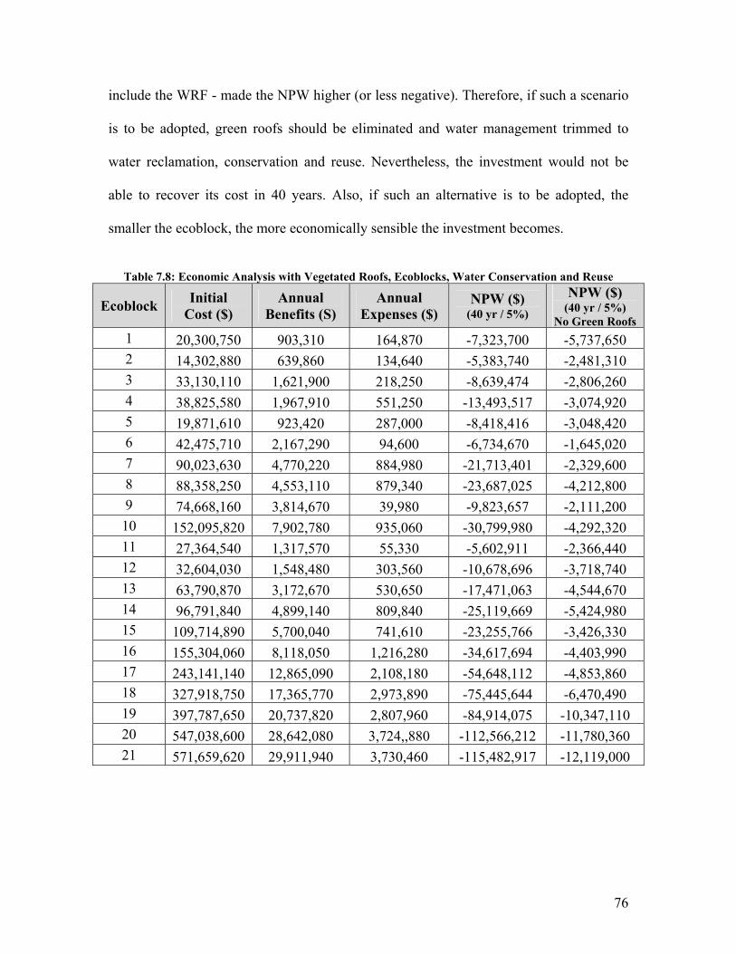
76

include the WRF - made the NPW higher (or less negative). Therefore, if such a scenario

is to be adopted, green roofs should be eliminated and water management trimmed to

water reclamation, conservation and reuse. Nevertheless, the investment would not be

able to recover its cost in 40 years. Also, if such an alternative is to be adopted, the

smaller the ecoblock, the more economically sensible the investment becomes.

Table 7.8: Economic Analysis with Vegetated Roofs, Ecoblocks, Water Conservation and Reuse

Ecoblock Initial Cost ($)

Annual Benefits (S)

Annual Expenses ($)

NPW ($) (40 yr / 5%)

NPW ($) (40 yr / 5%)

No Green Roofs1 20,300,750 903,310 164,870 -7,323,700 -5,737,650 2 14,302,880 639,860 134,640 -5,383,740 -2,481,310 3 33,130,110 1,621,900 218,250 -8,639,474 -2,806,260 4 38,825,580 1,967,910 551,250 -13,493,517 -3,074,920 5 19,871,610 923,420 287,000 -8,418,416 -3,048,420 6 42,475,710 2,167,290 94,600 -6,734,670 -1,645,020 7 90,023,630 4,770,220 884,980 -21,713,401 -2,329,600 8 88,358,250 4,553,110 879,340 -23,687,025 -4,212,800 9 74,668,160 3,814,670 39,980 -9,823,657 -2,111,200 10 152,095,820 7,902,780 935,060 -30,799,980 -4,292,320 11 27,364,540 1,317,570 55,330 -5,602,911 -2,366,440 12 32,604,030 1,548,480 303,560 -10,678,696 -3,718,740 13 63,790,870 3,172,670 530,650 -17,471,063 -4,544,670 14 96,791,840 4,899,140 809,840 -25,119,669 -5,424,980 15 109,714,890 5,700,040 741,610 -23,255,766 -3,426,330 16 155,304,060 8,118,050 1,216,280 -34,617,694 -4,403,990 17 243,141,140 12,865,090 2,108,180 -54,648,112 -4,853,860 18 327,918,750 17,365,770 2,973,890 -75,445,644 -6,470,490 19 397,787,650 20,737,820 2,807,960 -84,914,075 -10,347,110 20 547,038,600 28,642,080 3,724,,880 -112,566,212 -11,780,360 21 571,659,620 29,911,940 3,730,460 -115,482,917 -12,119,000

77

7.2.5- No Vegetated Roofs

Vegetated roofs had high installation or construction costs. Green-roofing an ecoblock

proved ten times more costly than a WRF in many ecoblocks which underlines the

importance of a scenario excluding vegetated roofs but including semiautonomous water

management, water and energy conservation and IRM. Table 7.9 shows the economic

analysis for this alternative. The initial cost now includes the cost of the WRF with heat

extraction and the annual expense includes their respective operational costs. Annual

benefits are now due mainly to water and energy conservation and reuse.

Table 7.9: Economic Analysis with No Green Roofs

Ecoblock Initial Cost ($)

Annual Benefits (S)

Annual Expenses ($)

NPW ($) (40 yr / 5%)

Payback Period (years)

1 4,633,910 1,647,940 744,900 10,861,350 6.0 2 4,191,340 1,235,420 608,320 6,569,200 8.5 3 5,467,640 2,450,440 986,080 19,659,400 4.5 4 10,063,590 4,459,320 2,490,610 23,717,640 6.0 5 6,429,010 2,056,720 1,296,710 6,612,120 11.5 6 4,282,790 3,016,980 427,410 40,151,970 2.0 7 15,605,520 8,886,120 3,998,420 68,262,960 3.5 8 15,423,470 8,108,660 3,972,960 55,541,430 4.5 9 5,183,780 4,261,970 180,630 64,848,310 1.5 10 17,482,110 13,061,850 4,224,700 134,155,390 2.0 11 3,501,170 1,557,220 249,990 18,929,640 3.0 12 6,825,640 2,891,260 1,371,500 19,252,120 5.5 13 10,350,010 5,349,690 2,397,540 40,306,150 4.0 14 14,589,170 8,119,110 3,658,930 61,943,450 3.5 15 14,579,250 9,805,170 3,350,650 96,174,540 2.5 16 21,465,690 14,610,280 5,495,290 134,939,340 2.5 17 34,884,660 23,479,630 9,524,960 204,564,840 2.5 18 47,683,750 31,533,380 13,436,340 262,845,200 3.0 19 48,068,260 35,216,260 12,686,630 338,519,880 2.5 20 62,705,510 48,269,840 16,829,380 476,784,430 2.5 21 63,463,160 49,747,300 16,854,580 500,946,380 2.0

78

The table above shows that this alternative has NPWs within 10% of the comprehensive

alternative of scenario 3 (section 7.2.3) and as such equally feasible. However, the PBPs

are about 10 years lower. That means that the cost of the WRF can be recovered

relatively quickly. This alternative is heavily dependent upon conservation and reuse

patterns as virtually all the savings come from energy and water savings. Therefore,

stakeholder participation and policies soliciting conservation are needed for the success

of this alternative. Generally, higher level ecoblocks showed faster payback periods

because of the strict reliance on conservation by the existing population. Nonetheless,

ecoblock 9 which had the lowest population density, no residences and dispersed

commercial and industrial buildings within, was bolstered by lower initial and operational

costs (relative to ecoblocks of a comparable area) and subsequently had the lowest PBP.

This means that this alternative, barring the difficulty in implementing it, is highly

adaptable to the environment in which it is implemented.

7.3- Analysis and Discussion

The LCCA was a necessary step in order to determine the feasibility of the different

alternatives proposed in the previous section. The TBL assessment tabulates social,

economical and environmental benefits for an alternative but does not account for initial

or operational costs. As such, the LCCA complements the TBL assessment by providing

further information and determining whether the proposed plan is economically viable. In

section 7.2, five scenarios were proposed and economically analyzed for their NPWs and

PBPs when applicable:

1) A green-roof-centric approach which is solely based on widespread vegetated

roofs application. This alternative proved to be unfeasible at the estimated

79

construction costs and current energy prices. Reductions in construction costs or

hikes in energy costs could make green-roofing feasible over the life-cycle of 40

years.

2) An energy-centric scenario which combines the two most efficient ways in this

study to conserve energy: direct energy conservation and green roofs. This

alternative showed that when green-roofs are integrated in an energy conservation

plan, the construction cost can be recovered in about 18 years and a positive

present worth can be calculated over the life-cycle.

3) A comprehensive approach which combines all the components of sustainable

resource management: decentralized water reclamation facilities, water and

energy conservation, vegetated roofs and alternative energy. This alternative was

also feasible and more suited for citywide management plans.

4) A water-centric alternative which revolves around water conservation,

reclamation and reuse. When combined with green roofs for stormwater retention,

this alternative proved highly unfeasible due to increased initial costs and

insufficient yearly savings. Without green-roofs, this alternative was more

numerically feasible, notably for small ecoblocks, but still had negative present

values. Therefore this alternative would probably work best in communitywide

management plans, or medium to large housing projects. It could also be

5) A conservation-centric approach or a no-green roofs approach that shuns the high

construction cost of green-roofs. Combining both water and energy conservation,

this was the most profitable alternative and can be applied to all types of

development or ecoblocks with varied land use covers. It is however strongly

80

contingent upon regulations and policies soliciting conversation of energy and

water and/or active stakeholder participation.

Figures 7.2 and 7.3 plot the results of the LCCA for the considered alternatives.

-100,000,000

0

100,000,000

200,000,000

300,000,000

400,000,000

500,000,000

600,000,000

0 1 2 3 4 5 6 7 8 9 10 11 12 13 14 15 16 17 18 19 20 21

Ecoblock

NPW

($)

Green-Roof-CentricEnergy-CentricComprehensiveWater-CentricConservation-Centric

Figure 7.2: NPW of the Five Scenarios in the Ecobloks

0

5

10

15

20

25

30

35

40

0 1 2 3 4 5 6 7 8 9 10 11 12 13 14 15 16 17 18 19 20 21Ecoblock

Payb

ack

Peri

od (y

ears

)

Energy-CentricComprehensiveConservation-Centric

Figure 7.3: Payback Period of the Three Feasible Scenarios in the Ecoblocks

81

Figure 7.2 shows greater benefits for larger ecoblocks with energy-centric, conservation-

centric and comprehensive approaches and less losses for smaller ecoblocks with green-

roof and water-centric approaches. Also, the two figures suggest that a

conservation/reclamation/reuse approach is the most profitable and the best in paying for

itself [Note that this scenario doesn’t take into account the cost of initiating a

conservation policy or program]. But what figures 7.2 and 7.3 fail to show is the effect of

the properties of each ecoblock on the results. Basically, the NPWs and the PBPs are

influenced by:

- the land use cover which affects the water consumption and conservation as well

as the presence of a sufficient building footprint area, a necessary matrix for green

roofs and their energy and water related benefits.

- the population density in the ecoblock which affects the water supply

requirements, the initial and operational costs of the water reclamation facility and

the benefits from water conservation.

Those two factors can act concordantly in that a high developed land covers (residential,

commercial, industrial) yields both a larger population and more surfaces for green roofs

and as such favors an alternative which integrates green roofs, conservation and water

reclamation. But the two factors can act discordantly in that a larger population density

may not directly result in a larger developed surface or larger green roof surface (e.g.

high rise buildings, tower housing, …) and in that case the benefits from conservation

might outweigh those from green roofs and an alternative that is centered on conservation

would become more profitable. Moreover, a large developed land cover results in a

reduced cover for open urban space such as parks and green corridors, a necessary

82

requirement for low impact development. As well, a larger population density causes

higher operational costs within the ecoblock. In order to better understand those

relationships, the NPWs and PBPs were plotted against the %Developed and the

population density in the ecoblocks. Those plots are shown in figures 7.4 to 7.7 for the

alternatives that proved to be feasible.

0

100,000,000

200,000,000

300,000,000

400,000,000

500,000,000

600,000,000

20 30 40 50 60 70 80 90 100% Developed

NPW

($)

Energy-CentricComprehensiveConservation-Centric

Figure 7.4: NPW versus % Developed

0

5

10

15

20

25

30

35

40

20 30 40 50 60 70 80 90 100% Developed

Payb

ack

Peri

od (y

ears

)

Energy-CentricComprehensiveConservation-CentricLinear (Energy-Centric)Linear (Comprehensive)Linear (Conservation-Centric)

Figure 7.5: PBP versus % Developed

83

0

100,000,000

200,000,000

300,000,000

400,000,000

500,000,000

600,000,000

1,000 3,000 5,000 7,000 9,000 11,000 13,000 15,000 17,000 19,000Population Density (persons/km2)

NPW

($)

Energy-CentricComprehensiveConservation-Centric

Figure 7.6: NPW versus Population Density

0

5

10

15

20

25

30

35

40

1,000 3,000 5,000 7,000 9,000 11,000 13,000 15,000 17,000 19,000Population Density (persons/km2)

Payb

ack

Peri

od (y

ears

)

Energy-CentricComprehensiveConservation-CentricLinear (Energy-Centric)Linear (Comprehensive)Linear (Conservation-Centric)

Figure 7.7: PBP versus Population Density

The effect of the percentage of developed land cover may be observed in figure 7.4 as the

NPW is highest in the range of 55 to 70%. This implies that there is enough matrix for

vegetated roofs to generate benefits while leaving a percentage for open space and

transportation related land uses. This also signifies the presence of enough people with

whom conservation can produce sufficient savings. For a percentage exceeding 70%, the

84

NPW drops as the installation cost for green roofs and the operational expenses of the

WRF possibly become significant. These effects, however, are not observed with the

payback period as trendlines added to the data showed that there’s hardly any variation

with the developed land cover except for a slight decline along the trendline for the

energy-centric alternative due to increased costs for green roofs for highly developed

ecoblocks.

On the other hand, the effect of the population density is less observed with the values

obtained with the clustering in chapter 2. Most of the values were in the range of 6000-

9000 people/km2 and as such the data in figures 7.6 and 7.7 may not be conclusive.

Nevertheless, one can still make the observation that relatively low NPWs exist at the

ends of the range of population densities. Also the presence of a large number of points

with high NPWs in the 6000-9000 people/km2 range may suggest that with more proper

clustering, points should line up in a curve resembling the normal distribution. Since low

densities create a reduced potential for savings from conservation and high densities

would contribute to high installation and operation costs for alternative energy, water

reclamation and vegetated roofs, median population densities would probably be the best

bet for developments adhering to principles of sustainable management. Another possible

noteworthy observation is that for the densities with the best NPWs in figure 7.6, the

points for comprehensive and conservation-centric alternatives tend to breakaway from

the points of the energy-centric approach. Since the difference is mainly due to

reclamation, conservation and reuse, all of which are contingent upon an adequate

population presence, it can be referred that at least these points are in deed in an

appropriate range of population density. As for the payback period, there is little

85

observed effect with comprehensive and conservation-centric alternatives but better

payback with higher densities for energy-centric approaches. The reason could be that the

energy-centric scenario in this study does not have any operational costs and as such

higher population does not directly translate into higher operational costs.

86

CHAPTER 8

CONCLUSIONS AND FINAL THOUGHTS

This study was mainly concerned with investigating the feasibility of sustainable

development in urban environments, implemented through an integrated resource plan

including water and energy conservation, vegetated roofs for stormwater retention and

building insulation, decentralized water management using water reclamation facilities in

semiautonomous clusters, and further resource management by heat extraction from

wastewater. Water and energy conservation were thoroughly dealt with and broken down

to direct and indirect ways to conserve, while proposing changes or items with no or

minimal additional cost. Green roofs were studied from the perspectives of water

retention, runoff reduction and building insulation. It was deduced, in a separate analysis,

that vegetated roofs are highly effective in reducing runoff from the one-year storm.

However, for larger design storms there’s a need to couple green roofs with other tools

that reduce directly connected impervious areas. For water reclamation, facilities using

biological nutrient removal and yielding a high quality reusable effluent were proposed

inside the urban ecoblocks with their cost estimated from construction curves. Land use

affected the computation of water supply, the size of the reclamation facility and the

potential for water conservation. Integrated resource management which aims at using

waste as a resource for energy as well as reducing the waste stream, was also considered.

Hence, anaerobic digestion and biogas production, along with heat extraction were

studied. TBL and LCC assessments put together the building blocks of the management

plans into coherent approaches. The TBL assessment was used to evaluate the proposed

87

plan by listing how it contributes to enhancing the social, environmental and economic

aspects of the community.

The TBL assessment revealed that the amount of water retained by green roofs exceeds

the amount of water conserved by efficient indoor appliances, and that about 95% of the

savings are energy related. This means that the potential to conserve energy is greater

than that of water, a stipulation that is propped up by the fact that LEED points in the

LEED rating system mostly deal with energy conservation rather than water. Also, since

savings from indirect conservation (resulting from water) were far less than those from

direct energy conservation, a policy that conserves energy strictly by conserving water

would fall short in terms of benefits in spite of the tight water-energy relationship

described by the “Water-Energy Nexus”.

Moreover, within the framework of LEED (Leadership in Energy and Environmental

Design), mandatory statutory constraints stemming from the TBL criteria have been

incorporated therein (Novotny, 2007). For example, US Green Building Council requires

30% indoor and 50% outdoor water savings, as well as stormwater controls, reclaimed

water use, and innovative approaches to treatment. With proper application of the

proposed practices and policies, sustainable management could earn a developer 14

energy efficiency points out of 17 (optimized energy performance, on-site renewable

energy and green power), 3 water efficiency points out of 5 (water efficient landscaping

and water use reduction) and some points for site development and stormwater control, in

the ratings for new building construction (i.e. about 20 points out 69 possible points).

However, in LEED ratings for new neighborhood developments, water and energy

efficiency with stormwater control, reclamation and reuse can only earn 10-12 points out

88

of 106 possible points, as most ratings for neighborhood developments revolve around

accessibility, location, affordability and ecological preservation. Therefore, sustainable

management is not well incorporated into LEED for neighborhood development, even

though it’s a paradigm that is targeted more for general urban planning rather than

specific buildings. Furthermore, another concern with the LEED standards is that they

don’t reflect the amount of improvement in environmental performance, neither the cost

associated with each credit. For example, developers can earn the same number of points

for a bicycle storage room and a 20% reduction in water use, or even a mere 5% in

materials use. Therefore, despite having some TBL criteria interspersed in the LEED

ratings, a TBL assessment (with LCCA) remains a more suited approach to determine the

extent to which a certain development or trend of development would play a part in a

sustainable water and energy management.

The relationship between water and energy also affects the way to configure them in one

policy. LCCA proved that an energy-centric approach that serves the purpose of energy

conservation and optimization is economically viable for both neighborhood size projects

and citywide projects whereas a water-centric approach does not generate enough

benefits to be adopted as a paradigm for large scale urban developments. This approach

may work for neighborhood, housing or community scale projects where cost of water

reclamation will be reduced. Thus, the LLCA suggest that the water-energy nexus is not

marked by equivalence, and is rather unidirectional. Energy-centric policies may not be

contingent upon efficient water management, but a water-centric policy needs a certain

element of energy efficiency to render it economically feasible. This stipulation,

however, may not be applicable in regions suffering from water shortage such as the

89

Southwest of the United States, the Arab Peninsula and Australia. Relative water

abundance in the Northeast states, results in relatively lower costs for water treatment and

reclamation, but high costs in water-shorted entities - due to costly treatments such as

reverse osmosis for seawater desalination and ultrafiltration - could mean that water

conservation benefits are much greater and a water centric approach might work. The

added energy requirements of advanced treatment may also impart the water-energy

nexus with more equivalence.

Conceivably, the water-energy relationship wouldn’t be of greater significance when both

resources are combined into one policy. The LCCA proved that a comprehensive

alternative integrating all of the components in this study and a conservation-centric

approach are the most economically viable and suitable for all sizes of ecoblocks. This

directly relates to the fact that the best strategy for sustainable and resilient urban

watersheds is a holistic paradigm that congregates and optimizes interdependent elements

into a well-targeted policy (Novotny, 2007). Conversely, a strategy concerned with a

“part” rather than the “whole” wouldn’t be as effective, as shown by a green-roof-centric

alternative which focuses only on the benefits of green-roofs. Such an alternative did not

generate enough benefits to recover the cost of green roofs over their life-cycle and

needed reduced construction costs or increased energy prices (both of which might not be

implausible) in order to become feasible.

Factors that affect the choice of an alternative as well as its efficacy are the size of the

target area or the ecoblock, the land use within the ecoblock and the population density.

This study established with a good level of confidence that sustainable management is

feasible but to a lesser level of certainty the most adequate properties of an ecoblock.

90

While the payback period was less dependent on the developed land cover and the

population density, the NPW showed high values at 55-70% developed land and a

population density in the range of 6000-9000 persons/km2. A minimum %development

that ensures the presence of enough roof surfaces and a minimum population density that

ensures enough potential for savings from conservation and reuse are needed. Large

densities and roof surfaces may contribute to high operational costs for heat extraction

and water reclamation and a reduced land cover for green ecotones and open spaces

which inflicts on the environment and the quality of life. As with any feasibility study,

the figure and conclusions are not definitive. Sources of potential errors and uncertainties

in this study include and may not be limited to:

- Avoided costs or costs that would have been spent were it for the proposed management

plan. Examples include the cost of urban BMPs (e.g. ponds) that would produce the same

reductions in urban runoff as green roofs, the cost of water that is used to replenish the

groundwater table and prevent subsidence, as well the cost associated with reducing the

GHG levels. Avoided costs constitute unqualified economic benefits.

- Unquantified costs or costs that were not included due to difficulties in doing so or lack

of data. For instance, sludge handling at the cluster WRFs may still be centralized at a

specific facility and could necessitate an additional cost that accounts for transport of

sludge to the treatment location.

- The clustering itself. A city can be clustered in an infinite number of ways and some

clustering methods could be more efficient than others. Future research studies may focus

on the clustering; possibly through an advanced GIS model that incorporates this

91

methodology and studies the variability of the results with different layouts of the

ecoblocks.

- Uncertainties with the distribution of the heat extraction system. Heat extraction is a

relatively new technology and as such it would be challenging to get exact estimates of

the installation and maintenance costs of a heat extraction system. These numbers may

vary between regions and states, and also depend on the heat extraction network itself.

This study assumes centralized heat extraction at the WRF where the heat is used

proximately or locally within the facility (e.g. to heat the digesters). However, the

Rabtherm system can be installed in a decentralized manner such as at every large

commercial building where the heat is used within the corresponding relevant building.

Such a scenario would have a different cost for IRM in the ecoblocks.

Further research might also quantify - for a specific management plan - with

mathematical formulas and models the relationships between the NPW or PBP and the

population density, the %green, the %developed and the size of the ecoblock, possibly

using data from different cities. The methodology used in this study for Boston, MA is

directly applicable in other cities. Parameters that would need to be changed are the land

use percentages, the costs of treating water and wastewater, the cost of providing energy

and locational multipliers. Other studies could also integrate resource management with

alternative transportation, rapid transit and solar energy. Resource management

assessments can also be performed on a well defined area of development (such a

university campus or a housing project) where other green design elements such as

porous pavement and bioswales can be implemented; conservation can be tailored

92

specifically to the occupancy and land use of the development, and water reclamation and

biogas production can be performed using small decentralized systems.

Another area which can be addressed is the financing of sustainable management and

how it affects the NPWs of the proposed alternatives. This study proved that sustainable

management can pay for itself but there could be additional costs to initiate resource

management programs and policies, and overcome the present barriers to their

implementation. For example, stakeholder participation through conservation may need

awareness programs and enacting new policies that need monitoring and follow up.

Speers (2007) referred to an analysis by Lindblom (1959) when he termed current

decision making a “successive limited comparison” or “muddling-through” since

administrators do not perform a comprehensive study of every option but rather look only

at policies that differ in small degrees with the ones currently in effect. Speers identified

this as a major administrative impediment, while Novotny and Brown (2007) also

warmed that there are significant economic and institutional barriers that need to be

overcome through education, new legislations, stakeholder participation and innovative

financing mechanisms.

93

APPENDIX A

EXTRACTS FROM IPCC REPORT 2007

Figure A.1: Atmospheric

concentrations of carbon dioxide,

methane and nitrous oxide over the last 10,000 years (large panels) and since

1750 (inset panels). (IPCC, 2007)

94

Figure A.2: Observed changes in global average surface temperature, global average sea level rise and Northern Hemisphere snow cover. Smoothed curves represent decadal

averaged values while circles show yearly values and the shaded areas are the uncertainty intervals (IPCC, 2007)

95

APPENDIX B

LAND USE CODE DEFINITIONS

Code Category Definition

1 Cropland Intensive agriculture 2 Pasture Extensive agriculture 3 Forest Forest 4 Wetland Nonforested freshwater wetland 5 Mining Sand; gravel & rock 6 Open Land Abandoned agriculture; power lines; areas of no vegetation

7 Participation Recreation Golf; tennis; Playgrounds; skiing

8 Spectator Recreation Stadiums; racetracks; Fairgrounds; drive-ins

9 Water Based Recreation Beaches; marinas; Swimming pools

10 Residential Multi-family 11 Residential Smaller than 1/4 acre lots 12 Residential 1/4 - 1/2 acre lots 13 Residential Larger than 1/2 acre lots 14 Salt Wetland Salt marsh 15 Commercial General urban; shopping center 16 Industrial Light & heavy industry

17 Urban Open Parks; cemeteries; public & institutional greenspace; also vacant undeveloped land

18 Transportation Airports; docks; divided highway; freight; storage; railroads 19 Waste Disposal Landfills; sewage lagoons 20 Water Fresh water; coastal embayment 21 Woody Perennial Orchard; nursery; cranberry bog 22 No Change Code used by MassGIS only during quality checking

(http://www.mass.gov/mgis/lus.htm)

96

APPENDIX C

DATA ON ENERGY REQUIREMENTS FOR WATER

CONVEYANCE AND TREATMENT

Table C.1: Cumulative Energy use in New England (Wilson, 2008) Treatment Level Cumulative Energy (kWh/MG)

Water Supply and Treatment 1800 + Distribution 2470

+ Preliminary Treatment 3170 + Secondary Treatment 4470

+ Advanced Treatment with Nitrogen Removal 6370 + MBR (to reclaim water and reuse it) 10470

Figure C.1: Energy Usage for Water Treatment and Distribution (AWWA, 1992)

97

Table C.2: Regional Water treatment and Pumping Costs (AWWA, 1992)

98

APPENDIX D

2005 – 2007 PRECIPITATION SERIES FOR BOSTON WITH

RETAINED DEPTH BY GREEN ROOFS

Date P (in) P (cm) Retained

Depth (cm) Date P (in) P (cm) Retained Depth (cm)

1/1/2005 0 0.0000 0.0000 2/1/2005 0 0.0000 0.00001/2/2005 0.02 0.0508 0.0447 2/2/2005 0 0.0000 0.00001/3/2005 0.18 0.4572 0.4023 2/3/2005 0.23 0.5842 0.51411/4/2005 0.29 0.7366 0.6482 2/4/2005 0.04 0.1016 0.08941/5/2005 0.1 0.2540 0.2235 2/5/2005 0.01 0.0254 0.02241/6/2005 0.64 1.6256 1.4305 2/6/2005 0 0.0000 0.00001/7/2005 0 0.0000 0.0000 2/7/2005 0 0.0000 0.00001/8/2005 0.58 1.4732 1.2964 2/8/2005 0 0.0000 0.00001/9/2005 0 0.0000 0.0000 2/9/2005 0.01 0.0254 0.0224

1/10/2005 0.03 0.0762 0.0671 2/10/2005 0.86 2.1844 1.92231/11/2005 0.01 0.0254 0.0224 2/11/2005 0 0.0000 0.00001/12/2005 0.29 0.7366 0.6482 2/12/2005 0 0.0000 0.00001/13/2005 0.05 0.1270 0.1118 2/13/2005 0 0.0000 0.00001/14/2005 0.44 1.1176 0.9835 2/14/2005 0.03 0.0762 0.06711/15/2005 0.01 0.0254 0.0224 2/15/2005 0.32 0.8128 0.71531/16/2005 0.05 0.1270 0.1118 2/16/2005 0.19 0.4826 0.42471/17/2005 0 0.0000 0.0000 2/17/2005 0 0.0000 0.00001/18/2005 0 0.0000 0.0000 2/18/2005 0 0.0000 0.00001/19/2005 0.07 0.1778 0.1565 2/19/2005 0 0.0000 0.00001/20/2005 0.01 0.0254 0.0224 2/20/2005 0.01 0.0254 0.02241/21/2005 0 0.0000 0.0000 2/21/2005 0.09 0.2286 0.20121/22/2005 0.18 0.4572 0.4023 2/22/2005 0.03 0.0762 0.06711/23/2005 0.26 0.6604 0.5812 2/23/2005 0 0.0000 0.00001/24/2005 0 0.0000 0.0000 2/24/2005 0.11 0.2794 0.24591/25/2005 0 0.0000 0.0000 2/25/2005 0.06 0.1524 0.13411/26/2005 0.2 0.5080 0.4470 2/26/2005 0 0.0000 0.00001/27/2005 0 0.0000 0.0000 2/27/2005 0 0.0000 0.00001/28/2005 0 0.0000 0.0000 2/28/2005 0.17 0.4318 0.38001/29/2005 0 0.0000 0.0000 4/1/2005 0.01 0.0254 0.02241/30/2005 0 0.0000 0.0000 4/2/2005 0.81 2.0574 1.81051/31/2005 0 0.0000 0.0000 4/3/2005 0.44 1.1176 0.98353/1/2005 0.11 0.2794 0.2459 4/4/2005 0 0.0000 0.00003/2/2005 0 0.0000 0.0000 4/5/2005 0 0.0000 0.00003/3/2005 0 0.0000 0.0000 4/6/2005 0 0.0000 0.00003/4/2005 0 0.0000 0.0000 4/7/2005 0.08 0.2032 0.17883/5/2005 0 0.0000 0.0000 4/8/2005 0.21 0.5334 0.46943/6/2005 0 0.0000 0.0000 4/9/2005 0 0.0000 0.00003/7/2005 0 0.0000 0.0000 4/10/2005 0 0.0000 0.00003/8/2005 0.49 1.2446 1.0952 4/11/2005 0 0.0000 0.00003/9/2005 0 0.0000 0.0000 4/12/2005 0.04 0.1016 0.0894

3/10/2005 0.01 0.0254 0.0224 4/13/2005 0 0.0000 0.00003/11/2005 0 0.0000 0.0000 4/14/2005 0 0.0000 0.00003/12/2005 0.8 2.0320 1.7882 4/15/2005 0.01 0.0254 0.02243/13/2005 0 0.0000 0.0000 4/16/2005 0 0.0000 0.00003/14/2005 0 0.0000 0.0000 4/17/2005 0 0.0000 0.00003/15/2005 0 0.0000 0.0000 4/18/2005 0 0.0000 0.00003/16/2005 0 0.0000 0.0000 4/19/2005 0 0.0000 0.00003/17/2005 0 0.0000 0.0000 4/20/2005 0.03 0.0762 0.06713/18/2005 0 0.0000 0.0000 4/21/2005 0.07 0.1778 0.15653/19/2005 0 0.0000 0.0000 4/22/2005 0 0.0000 0.00003/20/2005 0 0.0000 0.0000 4/23/2005 0.49 1.2446 1.09523/21/2005 0 0.0000 0.0000 4/24/2005 0.3 0.7620 0.6706

99

3/22/2005 0 0.0000 0.0000 4/25/2005 0.06 0.1524 0.13413/23/2005 0.04 0.1016 0.0894 4/26/2005 0 0.0000 0.00003/24/2005 0.15 0.3810 0.3353 4/27/2005 0.32 0.8128 0.71533/25/2005 0 0.0000 0.0000 4/28/2005 0 0.0000 0.00003/26/2005 0 0.0000 0.0000 4/29/2005 0 0.0000 0.00003/27/2005 0 0.0000 0.0000 4/30/2005 0.32 0.8128 0.71533/28/2005 1.3 3.3020 1.7831 6/1/2005 0 0.0000 0.00003/29/2005 0.49 1.2446 1.0952 6/2/2005 0 0.0000 0.00003/30/2005 0 0.0000 0.0000 6/3/2005 0 0.0000 0.00003/31/2005 0 0.0000 0.0000 6/4/2005 0 0.0000 0.00005/1/2005 0.1 0.2540 0.2235 6/5/2005 0.14 0.3556 0.31295/2/2005 0.04 0.1016 0.0894 6/6/2005 0.15 0.3810 0.33535/3/2005 0 0.0000 0.0000 6/7/2005 1 2.5400 1.37165/4/2005 0 0.0000 0.0000 6/8/2005 0.58 1.4732 1.29645/5/2005 0 0.0000 0.0000 6/9/2005 0.45 1.1430 1.00585/6/2005 0.04 0.1016 0.0894 6/10/2005 0 0.0000 0.00005/7/2005 0.56 1.4224 1.2517 6/11/2005 0 0.0000 0.00005/8/2005 0.05 0.1270 0.1118 6/12/2005 0 0.0000 0.00005/9/2005 0 0.0000 0.0000 6/13/2005 0 0.0000 0.0000

5/10/2005 0 0.0000 0.0000 6/14/2005 0 0.0000 0.00005/11/2005 0 0.0000 0.0000 6/15/2005 0.06 0.1524 0.13415/12/2005 0 0.0000 0.0000 6/16/2005 0.13 0.3302 0.29065/13/2005 0 0.0000 0.0000 6/17/2005 0.01 0.0254 0.02245/14/2005 0 0.0000 0.0000 6/18/2005 0 0.0000 0.00005/15/2005 0.01 0.0254 0.0224 6/19/2005 0.05 0.1270 0.11185/16/2005 0.27 0.6858 0.6035 6/20/2005 0 0.0000 0.00005/17/2005 0 0.0000 0.0000 6/21/2005 0 0.0000 0.00005/18/2005 0.04 0.1016 0.0894 6/22/2005 0.03 0.0762 0.06715/19/2005 0.01 0.0254 0.0224 6/23/2005 0 0.0000 0.00005/20/2005 0 0.0000 0.0000 6/24/2005 0.02 0.0508 0.04475/21/2005 0.23 0.5842 0.5141 6/25/2005 0 0.0000 0.00005/22/2005 0.03 0.0762 0.0671 6/26/2005 0.2 0.5080 0.44705/23/2005 0.06 0.1524 0.1341 6/27/2005 0 0.0000 0.00005/24/2005 0.92 2.3368 2.0564 6/28/2005 0 0.0000 0.00005/25/2005 0.74 1.8796 1.6540 6/29/2005 0 0.0000 0.00005/26/2005 0.54 1.3716 1.2070 6/30/2005 0 0.0000 0.00005/27/2005 0 0.0000 0.0000 8/1/2005 0.56 1.4224 1.25175/28/2005 0.16 0.4064 0.3576 8/2/2005 0.01 0.0254 0.02245/29/2005 0.13 0.3302 0.2906 8/3/2005 0 0.0000 0.00005/30/2005 0.04 0.1016 0.0894 8/4/2005 0 0.0000 0.00005/31/2005 0.01 0.0254 0.0224 8/5/2005 0.55 1.3970 1.22947/1/2005 0 0.0000 0.0000 8/6/2005 0 0.0000 0.00007/2/2005 0 0.0000 0.0000 8/7/2005 0 0.0000 0.00007/3/2005 0 0.0000 0.0000 8/8/2005 0 0.0000 0.00007/4/2005 0 0.0000 0.0000 8/9/2005 0.02 0.0508 0.04477/5/2005 0 0.0000 0.0000 8/10/2005 0 0.0000 0.00007/6/2005 2.04 5.1816 2.7981 8/11/2005 0.23 0.5842 0.51417/7/2005 0 0.0000 0.0000 8/12/2005 0 0.0000 0.00007/8/2005 0.95 2.4130 2.1234 8/13/2005 0.07 0.1778 0.15657/9/2005 0.2 0.5080 0.4470 8/14/2005 0.6 1.5240 1.3411

7/10/2005 0 0.0000 0.0000 8/15/2005 0.13 0.3302 0.29067/11/2005 0 0.0000 0.0000 8/16/2005 0 0.0000 0.00007/12/2005 0 0.0000 0.0000 8/17/2005 0 0.0000 0.00007/13/2005 0 0.0000 0.0000 8/18/2005 0 0.0000 0.00007/14/2005 0 0.0000 0.0000 8/19/2005 0 0.0000 0.00007/15/2005 0 0.0000 0.0000 8/20/2005 0 0.0000 0.00007/16/2005 0 0.0000 0.0000 8/21/2005 0.02 0.0508 0.04477/17/2005 0 0.0000 0.0000 8/22/2005 0 0.0000 0.00007/18/2005 0.03 0.0762 0.0671 8/23/2005 0 0.0000 0.00007/19/2005 0 0.0000 0.0000 8/24/2005 0 0.0000 0.00007/20/2005 0 0.0000 0.0000 8/25/2005 0 0.0000 0.00007/21/2005 0 0.0000 0.0000 8/26/2005 0 0.0000 0.00007/22/2005 0.15 0.3810 0.3353 8/27/2005 0 0.0000 0.00007/23/2005 0 0.0000 0.0000 8/28/2005 0 0.0000 0.00007/24/2005 0 0.0000 0.0000 8/29/2005 0.33 0.8382 0.73767/25/2005 0 0.0000 0.0000 8/30/2005 0.33 0.8382 0.73767/26/2005 0 0.0000 0.0000 8/31/2005 0.03 0.0762 0.06717/27/2005 0 0.0000 0.0000 10/1/2005 0 0.0000 0.00007/28/2005 0 0.0000 0.0000 10/2/2005 0 0.0000 0.0000

100

7/29/2005 0 0.0000 0.0000 10/3/2005 0 0.0000 0.00007/30/2005 0 0.0000 0.0000 10/4/2005 0 0.0000 0.00007/31/2005 0 0.0000 0.0000 10/5/2005 0 0.0000 0.00009/1/2005 0.19 0.4826 0.4247 10/6/2005 0 0.0000 0.00009/2/2005 0 0.0000 0.0000 10/7/2005 0.03 0.0762 0.06719/3/2005 0 0.0000 0.0000 10/8/2005 1.02 2.5908 1.39909/4/2005 0 0.0000 0.0000 10/9/2005 0.92 2.3368 2.05649/5/2005 0 0.0000 0.0000 10/10/2005 0.09 0.2286 0.20129/6/2005 0 0.0000 0.0000 10/11/2005 0.22 0.5588 0.49179/7/2005 0 0.0000 0.0000 10/12/2005 0.02 0.0508 0.04479/8/2005 0 0.0000 0.0000 10/13/2005 0.06 0.1524 0.13419/9/2005 0 0.0000 0.0000 10/14/2005 1.22 xxx xxx

9/10/2005 0 0.0000 0.0000 10/15/2005 2.89 10.4400 5.01129/11/2005 0 0.0000 0.0000 10/16/2005 0 0.0000 0.00009/12/2005 0 0.0000 0.0000 10/17/2005 0 0.0000 0.00009/13/2005 0 0.0000 0.0000 10/18/2005 0.02 0.0508 0.04479/14/2005 0 0.0000 0.0000 10/19/2005 0 0.0000 0.00009/15/2005 0.98 2.4892 2.1905 10/20/2005 0 0.0000 0.00009/16/2005 0.12 0.3048 0.2682 10/21/2005 0 0.0000 0.00009/17/2005 0.01 0.0254 0.0224 10/22/2005 0.64 1.6256 1.43059/18/2005 0 0.0000 0.0000 10/23/2005 0.46 1.1684 1.02829/19/2005 0 0.0000 0.0000 10/24/2005 0.11 0.2794 0.24599/20/2005 0.01 0.0254 0.0224 10/25/2005 1.26 3.2004 1.72829/21/2005 0 0.0000 0.0000 10/26/2005 0 0.0000 0.00009/22/2005 0 0.0000 0.0000 10/27/2005 0 0.0000 0.00009/23/2005 0 0.0000 0.0000 10/28/2005 0 0.0000 0.00009/24/2005 0 0.0000 0.0000 10/29/2005 0.45 1.1430 1.00589/25/2005 0 0.0000 0.0000 10/30/2005 0 0.0000 0.00009/26/2005 0.22 0.5588 0.4917 10/31/2005 0 0.0000 0.00009/27/2005 0.02 0.0508 0.0447 12/1/2005 0 0.0000 0.00009/28/2005 0 0.0000 0.0000 12/2/2005 0 0.0000 0.00009/29/2005 0.24 0.6096 0.5364 12/3/2005 0 0.0000 0.00009/30/2005 0 0.0000 0.0000 12/4/2005 0.12 0.3048 0.268211/1/2005 0 0.0000 0.0000 12/5/2005 0 0.0000 0.000011/2/2005 0 0.0000 0.0000 12/6/2005 0 0.0000 0.000011/3/2005 0 0.0000 0.0000 12/7/2005 0 0.0000 0.000011/4/2005 0 0.0000 0.0000 12/8/2005 0 0.0000 0.000011/5/2005 0 0.0000 0.0000 12/9/2005 0.63 1.6002 1.408211/6/2005 0.22 0.5588 0.4917 12/10/2005 0 0.0000 0.000011/7/2005 0.01 0.0254 0.0224 12/11/2005 0 0.0000 0.000011/8/2005 0 0.0000 0.0000 12/12/2005 0 0.0000 0.000011/9/2005 0.22 0.5588 0.4917 12/13/2005 0 0.0000 0.000011/10/2005 0.36 0.9144 0.8047 12/14/2005 0 0.0000 0.000011/11/2005 0.01 0.0254 0.0224 12/15/2005 0 0.0000 0.000011/12/2005 0.03 0.0762 0.0671 12/16/2005 0.64 1.6256 1.430511/13/2005 0 0.0000 0.0000 12/17/2005 0 0.0000 0.000011/14/2005 0 0.0000 0.0000 12/18/2005 0 0.0000 0.000011/15/2005 0.1 0.2540 0.2235 12/19/2005 0 0.0000 0.000011/16/2005 0.21 0.5334 0.4694 12/20/2005 0 0.0000 0.000011/17/2005 0.15 0.3810 0.3353 12/21/2005 0 0.0000 0.000011/18/2005 0 0.0000 0.0000 12/22/2005 0 0.0000 0.000011/19/2005 0 0.0000 0.0000 12/23/2005 0 0.0000 0.000011/20/2005 0 0.0000 0.0000 12/24/2005 0 0.0000 0.000011/21/2005 0.16 0.4064 0.3576 12/25/2005 0.21 0.5334 0.469411/22/2005 1.61 4.0894 2.2083 12/26/2005 0.77 1.9558 1.721111/23/2005 0.02 0.0508 0.0447 12/27/2005 0 0.0000 0.000011/24/2005 0.03 0.0762 0.0671 12/28/2005 0 0.0000 0.000011/25/2005 0 0.0000 0.0000 12/29/2005 0.24 0.6096 0.536411/26/2005 0 0.0000 0.0000 12/30/2005 0 0.0000 0.000011/27/2005 0 0.0000 0.0000 12/31/2005 0.05 0.1270 0.111811/28/2005 0 0.0000 0.000011/29/2005 0 0.0000 0.000011/30/2005 0.64 1.6256 1.4305

1/1/2006 0 0.0000 0.0000 2/1/2006 0 0.0000 0.00001/2/2006 0.02 0.0508 0.0447 2/2/2006 0 0.0000 0.00001/3/2006 0.18 0.4572 0.4023 2/3/2006 0.61 1.5494 1.36351/4/2006 0.29 0.7366 0.6482 2/4/2006 0.45 1.1430 1.00581/5/2006 0.1 0.2540 0.2235 2/5/2006 0.34 0.8636 0.7600

101

1/6/2006 0.64 1.6256 1.4305 2/6/2006 0 0.0000 0.00001/7/2006 0 0.0000 0.0000 2/7/2006 0 0.0000 0.00001/8/2006 0.58 1.4732 1.2964 2/8/2006 0 0.0000 0.00001/9/2006 0 0.0000 0.0000 2/9/2006 0 0.0000 0.0000

1/10/2006 0.03 0.0762 0.0671 2/10/2006 0 0.0000 0.00001/11/2006 0.01 0.0254 0.0224 2/11/2006 0 0.0000 0.00001/12/2006 0.29 0.7366 0.6482 2/12/2006 0.17 0.4318 0.38001/13/2006 0.05 0.1270 0.1118 2/13/2006 0 0.0000 0.00001/14/2006 0.44 1.1176 0.9835 2/14/2006 0 0.0000 0.00001/15/2006 0.01 0.0254 0.0224 2/15/2006 0 0.0000 0.00001/16/2006 0.05 0.1270 0.1118 2/16/2006 0 0.0000 0.00001/17/2006 0 0.0000 0.0000 2/17/2006 0.08 0.2032 0.17881/18/2006 0 0.0000 0.0000 2/18/2006 0 0.0000 0.00001/19/2006 0.07 0.1778 0.1565 2/19/2006 0 0.0000 0.00001/20/2006 0.01 0.0254 0.0224 2/20/2006 0 0.0000 0.00001/21/2006 0 0.0000 0.0000 2/21/2006 0 0.0000 0.00001/22/2006 0.18 0.4572 0.4023 2/22/2006 0 0.0000 0.00001/23/2006 0.26 0.6604 0.5812 2/23/2006 0.05 0.1270 0.11181/24/2006 0 0.0000 0.0000 2/24/2006 0 0.0000 0.00001/25/2006 0 0.0000 0.0000 2/25/2006 0.02 0.0508 0.04471/26/2006 0.2 0.5080 0.4470 2/26/2006 0 0.0000 0.00001/27/2006 0 0.0000 0.0000 2/27/2006 0 0.0000 0.00001/28/2006 0 0.0000 0.0000 2/28/2006 0.01 0.0254 0.02241/29/2006 0 0.0000 0.0000 4/1/2006 0.06 0.1524 0.13411/30/2006 0 0.0000 0.0000 4/2/2006 0 0.0000 0.00001/31/2006 0 0.0000 0.0000 4/3/2006 0.05 0.1270 0.11183/1/2006 0 0.0000 0.0000 4/4/2006 0.36 0.9144 0.80473/2/2006 0 0.0000 0.0000 4/5/2006 0.2 0.5080 0.44703/3/2006 0 0.0000 0.0000 4/6/2006 0 0.0000 0.00003/4/2006 0 0.0000 0.0000 4/7/2006 0.11 0.2794 0.24593/5/2006 0 0.0000 0.0000 4/8/2006 0.12 0.3048 0.26823/6/2006 0 0.0000 0.0000 4/9/2006 0 0.0000 0.00003/7/2006 0 0.0000 0.0000 4/10/2006 0 0.0000 0.00003/8/2006 0 0.0000 0.0000 4/11/2006 0 0.0000 0.00003/9/2006 0 0.0000 0.0000 4/12/2006 0 0.0000 0.0000

3/10/2006 0 0.0000 0.0000 4/13/2006 0.01 0.0254 0.02243/11/2006 0 0.0000 0.0000 4/14/2006 0.03 0.0762 0.06713/12/2006 0 0.0000 0.0000 4/15/2006 0 0.0000 0.00003/13/2006 0.3 0.7620 0.6706 4/16/2006 0 0.0000 0.00003/14/2006 0.25 0.6350 0.5588 4/17/2006 0.01 0.0254 0.02243/15/2006 0 0.0000 0.0000 4/18/2006 0.01 0.0254 0.02243/16/2006 0 0.0000 0.0000 4/19/2006 0 0.0000 0.00003/17/2006 0 0.0000 0.0000 4/20/2006 0 0.0000 0.00003/18/2006 0 0.0000 0.0000 4/21/2006 0 0.0000 0.00003/19/2006 0 0.0000 0.0000 4/22/2006 0.11 0.2794 0.24593/20/2006 0 0.0000 0.0000 4/23/2006 0.61 1.5494 1.36353/21/2006 0 0.0000 0.0000 4/24/2006 0.13 0.3302 0.29063/22/2006 0 0.0000 0.0000 4/25/2006 0.02 0.0508 0.04473/23/2006 0 0.0000 0.0000 4/26/2006 0 0.0000 0.00003/24/2006 0 0.0000 0.0000 4/27/2006 0 0.0000 0.00003/25/2006 0.01 0.0254 0.0224 4/28/2006 0 0.0000 0.00003/26/2006 0 0.0000 0.0000 4/29/2006 0 0.0000 0.00003/27/2006 0 0.0000 0.0000 4/30/2006 0 0.0000 0.00003/28/2006 0 0.0000 0.0000 6/1/2006 0.14 0.3556 0.31293/29/2006 0 0.0000 0.0000 6/2/2006 0.53 1.3462 1.18473/30/2006 0 0.0000 0.0000 6/3/2006 1.91 4.8514 2.61983/31/2006 0 0.0000 0.0000 6/4/2006 0.3 0.7620 0.67065/1/2006 0.01 0.0254 0.0224 6/5/2006 0 0.0000 0.00005/2/2006 0.91 2.3114 2.0340 6/6/2006 0 0.0000 0.00005/3/2006 0.26 0.6604 0.5812 6/7/2006 2.89 7.3406 3.96395/4/2006 0 0.0000 0.0000 6/8/2006 0.2 0.5080 0.44705/5/2006 0 0.0000 0.0000 6/9/2006 0.06 0.1524 0.13415/6/2006 0 0.0000 0.0000 6/10/2006 0.43 1.0922 0.96115/7/2006 0 0.0000 0.0000 6/11/2006 0 0.0000 0.00005/8/2006 0 0.0000 0.0000 6/12/2006 0 0.0000 0.00005/9/2006 0.96 2.4384 2.1458 6/13/2006 0 0.0000 0.0000

5/10/2006 0.55 1.3970 1.2294 6/14/2006 0 0.0000 0.00005/11/2006 0.08 0.2032 0.1788 6/15/2006 0.1 0.2540 0.22355/12/2006 0.37 0.9398 0.8270 6/16/2006 0 0.0000 0.0000

102

5/13/2006 3.84 xxx xxx 6/17/2006 0 0.0000 0.00005/14/2006 3.77 19.3300 9.2784 6/18/2006 0 0.0000 0.00005/15/2006 0.36 0.9144 0.8047 6/19/2006 0 0.0000 0.00005/16/2006 0.52 1.3208 1.1623 6/20/2006 0.37 0.9398 0.82705/17/2006 0 0.0000 0.0000 6/21/2006 0 0.0000 0.00005/18/2006 0 0.0000 0.0000 6/22/2006 0 0.0000 0.00005/19/2006 0.47 1.1938 1.0505 6/23/2006 1.36 3.4544 1.86545/20/2006 0 0.0000 0.0000 6/24/2006 0.69 1.7526 1.54235/21/2006 0.11 0.2794 0.2459 6/25/2006 0.95 2.4130 2.12345/22/2006 0 0.0000 0.0000 6/26/2006 0 0.0000 0.00005/23/2006 0 0.0000 0.0000 6/27/2006 0 0.0000 0.00005/24/2006 0 0.0000 0.0000 6/28/2006 0.05 0.1270 0.11185/25/2006 0 0.0000 0.0000 6/29/2006 0 0.0000 0.00005/26/2006 0.27 0.6858 0.6035 6/30/2006 0.13 0.3302 0.29065/27/2006 0 0.0000 0.0000 8/1/2006 0.02 0.0508 0.04475/28/2006 0 0.0000 0.0000 8/2/2006 0 0.0000 0.00005/29/2006 0 0.0000 0.0000 8/3/2006 0 0.0000 0.00005/30/2006 0 0.0000 0.0000 8/4/2006 0.31 0.7874 0.69295/31/2006 0 0.0000 0.0000 8/5/2006 0 0.0000 0.00007/1/2006 0 0.0000 0.0000 8/6/2006 0 0.0000 0.00007/2/2006 0 0.0000 0.0000 8/7/2006 0.04 0.1016 0.08947/3/2006 0 0.0000 0.0000 8/8/2006 0 0.0000 0.00007/4/2006 0 0.0000 0.0000 8/9/2006 0 0.0000 0.00007/5/2006 0 0.0000 0.0000 8/10/2006 0 0.0000 0.00007/6/2006 0.15 0.3810 0.3353 8/11/2006 0 0.0000 0.00007/7/2006 0 0.0000 0.0000 8/12/2006 0 0.0000 0.00007/8/2006 0 0.0000 0.0000 8/13/2006 0 0.0000 0.00007/9/2006 0 0.0000 0.0000 8/14/2006 0 0.0000 0.0000

7/10/2006 0 0.0000 0.0000 8/15/2006 0.53 1.3462 1.18477/11/2006 0.02 0.0508 0.0447 8/16/2006 0 0.0000 0.00007/12/2006 1.02 2.5908 1.3990 8/17/2006 0 0.0000 0.00007/13/2006 0.17 0.4318 0.3800 8/18/2006 0 0.0000 0.00007/14/2006 0 0.0000 0.0000 8/19/2006 0 0.0000 0.00007/15/2006 0 0.0000 0.0000 8/20/2006 0.8 2.0320 1.78827/16/2006 0 0.0000 0.0000 8/21/2006 0 0.0000 0.00007/17/2006 0 0.0000 0.0000 8/22/2006 0 0.0000 0.00007/18/2006 0.22 0.5588 0.4917 8/23/2006 0 0.0000 0.00007/19/2006 0.19 0.4826 0.4247 8/24/2006 0.01 0.0254 0.02247/20/2006 0 0.0000 0.0000 8/25/2006 0.84 2.1336 1.87767/21/2006 1.29 3.2766 1.7694 8/26/2006 0 0.0000 0.00007/22/2006 0.12 0.3048 0.2682 8/27/2006 0.4 1.0160 0.89417/23/2006 0.11 0.2794 0.2459 8/28/2006 0.11 0.2794 0.24597/24/2006 0 0.0000 0.0000 8/29/2006 0.14 0.3556 0.31297/25/2006 0 0.0000 0.0000 8/30/2006 0 0.0000 0.00007/26/2006 0 0.0000 0.0000 8/31/2006 0 0.0000 0.00007/27/2006 0 0.0000 0.0000 10/1/2006 0.38 0.9652 0.84947/28/2006 0.29 0.7366 0.6482 10/2/2006 0 0.0000 0.00007/29/2006 0 0.0000 0.0000 10/3/2006 0 0.0000 0.00007/30/2006 0 0.0000 0.0000 10/4/2006 0 0.0000 0.00007/31/2006 0 0.0000 0.0000 10/5/2006 0.12 0.3048 0.26829/1/2006 0 0.0000 0.0000 10/6/2006 0 0.0000 0.00009/2/2006 0 0.0000 0.0000 10/7/2006 0 0.0000 0.00009/3/2006 0.25 0.6350 0.5588 10/8/2006 0 0.0000 0.00009/4/2006 0 0.0000 0.0000 10/9/2006 0 0.0000 0.00009/5/2006 0.07 0.1778 0.1565 10/10/2006 0 0.0000 0.00009/6/2006 0.01 0.0254 0.0224 10/11/2006 0.85 2.1590 1.89999/7/2006 0 0.0000 0.0000 10/12/2006 0.39 0.9906 0.87179/8/2006 0 0.0000 0.0000 10/13/2006 0 0.0000 0.00009/9/2006 0.22 0.5588 0.4917 10/14/2006 0 0.0000 0.0000

9/10/2006 0 0.0000 0.0000 10/15/2006 0 0.0000 0.00009/11/2006 0 0.0000 0.0000 10/16/2006 0 0.0000 0.00009/12/2006 0 0.0000 0.0000 10/17/2006 0.13 0.3302 0.29069/13/2006 0 0.0000 0.0000 10/18/2006 0 0.0000 0.00009/14/2006 0.3 0.7620 0.6706 10/19/2006 0 0.0000 0.00009/15/2006 0 0.0000 0.0000 10/20/2006 0.4 1.0160 0.89419/16/2006 0 0.0000 0.0000 10/21/2006 0 0.0000 0.00009/17/2006 0 0.0000 0.0000 10/22/2006 0 0.0000 0.00009/18/2006 0 0.0000 0.0000 10/23/2006 0.21 0.5334 0.46949/19/2006 0.5 1.2700 1.1176 10/24/2006 0 0.0000 0.0000

103

9/20/2006 0.07 0.1778 0.1565 10/25/2006 0 0.0000 0.00009/21/2006 0 0.0000 0.0000 10/26/2006 0 0.0000 0.00009/22/2006 0 0.0000 0.0000 10/27/2006 0 0.0000 0.00009/23/2006 0.04 0.1016 0.0894 10/28/2006 2.02 5.1308 2.77069/24/2006 0 0.0000 0.0000 10/29/2006 0 0.0000 0.00009/25/2006 0 0.0000 0.0000 10/30/2006 0 0.0000 0.00009/26/2006 0 0.0000 0.0000 10/31/2006 0 0.0000 0.00009/27/2006 0 0.0000 0.0000 12/1/2006 0.18 0.4572 0.40239/28/2006 0 0.0000 0.0000 12/2/2006 0 0.0000 0.00009/29/2006 0.48 1.2192 1.0729 12/3/2006 0 0.0000 0.00009/30/2006 0 0.0000 0.0000 12/4/2006 0.19 0.4826 0.424711/1/2006 0.09 0.2286 0.2012 12/5/2006 0 0.0000 0.000011/2/2006 0.23 0.5842 0.5141 12/6/2006 0 0.0000 0.000011/3/2006 0 0.0000 0.0000 12/7/2006 0 0.0000 0.000011/4/2006 0 0.0000 0.0000 12/8/2006 0 0.0000 0.000011/5/2006 0 0.0000 0.0000 12/9/2006 0 0.0000 0.000011/6/2006 0 0.0000 0.0000 12/10/2006 0 0.0000 0.000011/7/2006 0.14 0.3556 0.3129 12/11/2006 0 0.0000 0.000011/8/2006 1.19 3.0226 1.6322 12/12/2006 0 0.0000 0.000011/9/2006 0.08 0.2032 0.1788 12/13/2006 0.1 0.2540 0.223511/10/2006 0 0.0000 0.0000 12/14/2006 0 0.0000 0.000011/11/2006 0 0.0000 0.0000 12/15/2006 0 0.0000 0.000011/12/2006 0.45 1.1430 1.0058 12/16/2006 0.01 0.0254 0.022411/13/2006 0.52 1.3208 1.1623 12/17/2006 0 0.0000 0.000011/14/2006 0.35 0.8890 0.7823 12/18/2006 0.02 0.0508 0.044711/15/2006 0 0.0000 0.0000 12/19/2006 0 0.0000 0.000011/16/2006 0.15 0.3810 0.3353 12/20/2006 0 0.0000 0.000011/17/2006 0.49 1.2446 1.0952 12/21/2006 0 0.0000 0.000011/18/2006 0 0.0000 0.0000 12/22/2006 0.06 0.1524 0.134111/19/2006 0 0.0000 0.0000 12/23/2006 0.81 2.0574 1.810511/20/2006 0 0.0000 0.0000 12/24/2006 0 0.0000 0.000011/21/2006 0 0.0000 0.0000 12/25/2006 0.09 0.2286 0.201211/22/2006 0 0.0000 0.0000 12/26/2006 0.34 0.8636 0.760011/23/2006 1.83 4.6482 2.5100 12/27/2006 0 0.0000 0.000011/24/2006 0.27 0.6858 0.6035 12/28/2006 0 0.0000 0.000011/25/2006 0 0.0000 0.0000 12/29/2006 0 0.0000 0.000011/26/2006 0 0.0000 0.0000 12/30/2006 0.08 0.2032 0.178811/27/2006 0 0.0000 0.0000 12/31/2006 0 0.0000 0.000011/28/2006 0.01 0.0254 0.0224 11/29/2006 0 0.0000 0.000011/30/2006 0 0.0000 0.0000

1/1/2007 0.86 2.1844 1.9223 2/1/2007 0 0.0000 0.00001/2/2007 0 0.0000 0.0000 2/2/2007 0.19 0.4826 0.42471/3/2007 0 0.0000 0.0000 2/3/2007 0.06 0.1524 0.13411/4/2007 0 0.0000 0.0000 2/4/2007 0 0.0000 0.00001/5/2007 0.01 0.0254 0.0224 2/5/2007 0 0.0000 0.00001/6/2007 0.07 0.1778 0.1565 2/6/2007 0 0.0000 0.00001/7/2007 0 0.0000 0.0000 2/7/2007 0 0.0000 0.00001/8/2007 0.57 1.4478 1.2741 2/8/2007 0 0.0000 0.00001/9/2007 0 0.0000 0.0000 2/9/2007 0 0.0000 0.0000

1/10/2007 0 0.0000 0.0000 2/10/2007 0 0.0000 0.00001/11/2007 0 0.0000 0.0000 2/11/2007 0 0.0000 0.00001/12/2007 0 0.0000 0.0000 2/12/2007 0 0.0000 0.00001/13/2007 0.06 0.1524 0.1341 2/13/2007 0 0.0000 0.00001/14/2007 0.13 0.3302 0.2906 2/14/2007 1.62 4.1148 2.22201/15/2007 0.64 1.6256 1.4305 2/15/2007 0 0.0000 0.00001/16/2007 0.06 0.1524 0.1341 2/16/2007 0 0.0000 0.00001/17/2007 0 0.0000 0.0000 2/17/2007 0 0.0000 0.00001/18/2007 0 0.0000 0.0000 2/18/2007 0 0.0000 0.00001/19/2007 0 0.0000 0.0000 2/19/2007 0 0.0000 0.00001/20/2007 0 0.0000 0.0000 2/20/2007 0 0.0000 0.00001/21/2007 0 0.0000 0.0000 2/21/2007 0 0.0000 0.00001/22/2007 0.02 0.0508 0.0447 2/22/2007 0.02 0.0508 0.04471/23/2007 0 0.0000 0.0000 2/23/2007 0.01 0.0254 0.02241/24/2007 0 0.0000 0.0000 2/24/2007 0 0.0000 0.00001/25/2007 0 0.0000 0.0000 2/25/2007 0 0.0000 0.00001/26/2007 0 0.0000 0.0000 2/26/2007 0.3 0.7620 0.67061/27/2007 0 0.0000 0.0000 2/27/2007 0 0.0000 0.0000

104

1/28/2007 0.02 0.0508 0.0447 2/28/2007 0 0.0000 0.00001/29/2007 0 0.0000 0.0000 4/1/2007 0.17 0.4318 0.38001/30/2007 0 0.0000 0.0000 4/2/2007 0.15 0.3810 0.33531/31/2007 0 0.0000 0.0000 4/3/2007 0.01 0.0254 0.02243/1/2007 0 0.0000 0.0000 4/4/2007 0.94 2.3876 2.10113/2/2007 1.48 3.7592 2.0300 4/5/2007 0.27 0.6858 0.60353/3/2007 0 0.0000 0.0000 4/6/2007 0 0.0000 0.00003/4/2007 0 0.0000 0.0000 4/7/2007 0 0.0000 0.00003/5/2007 0 0.0000 0.0000 4/8/2007 0 0.0000 0.00003/6/2007 0 0.0000 0.0000 4/9/2007 0 0.0000 0.00003/7/2007 0 0.0000 0.0000 4/10/2007 0 0.0000 0.00003/8/2007 0 0.0000 0.0000 4/11/2007 0 0.0000 0.00003/9/2007 0 0.0000 0.0000 4/12/2007 0.87 2.2098 1.9446

3/10/2007 0 0.0000 0.0000 4/13/2007 0 0.0000 0.00003/11/2007 0.27 0.6858 0.6035 4/14/2007 0 0.0000 0.00003/12/2007 0 0.0000 0.0000 4/15/2007 1.42 3.6068 1.94773/13/2007 0 0.0000 0.0000 4/16/2007 0.93 2.3622 2.07873/14/2007 0 0.0000 0.0000 4/17/2007 0.16 0.4064 0.35763/15/2007 0.12 0.3048 0.2682 4/18/2007 0.05 0.1270 0.11183/16/2007 0.42 1.0668 0.9388 4/19/2007 0 0.0000 0.00003/17/2007 1.46 3.7084 2.0025 4/20/2007 0 0.0000 0.00003/18/2007 0 0.0000 0.0000 4/21/2007 0 0.0000 0.00003/19/2007 0.05 0.1270 0.1118 4/22/2007 0 0.0000 0.00003/20/2007 0.02 0.0508 0.0447 4/23/2007 0 0.0000 0.00003/21/2007 0 0.0000 0.0000 4/24/2007 0 0.0000 0.00003/22/2007 0 0.0000 0.0000 4/25/2007 0.17 0.4318 0.38003/23/2007 0 0.0000 0.0000 4/26/2007 0 0.0000 0.00003/24/2007 0.34 0.8636 0.7600 4/27/2007 1.06 2.6924 1.45393/25/2007 0 0.0000 0.0000 4/28/2007 0.37 0.9398 0.82703/26/2007 0.11 0.2794 0.2459 4/29/2007 0.06 0.1524 0.13413/27/2007 0.04 0.1016 0.0894 4/30/2007 0.08 0.2032 0.17883/28/2007 0 0.0000 0.0000 6/1/2007 0.15 0.3810 0.33533/29/2007 0 0.0000 0.0000 6/2/2007 0 0.0000 0.00003/30/2007 0 0.0000 0.0000 6/3/2007 0.11 0.2794 0.24593/31/2007 0 0.0000 0.0000 6/4/2007 1.46 3.7084 2.00255/1/2007 0 0.0000 0.0000 6/5/2007 0 0.0000 0.00005/2/2007 0.08 0.2032 0.1788 6/6/2007 0 0.0000 0.00005/3/2007 0 0.0000 0.0000 6/7/2007 0 0.0000 0.00005/4/2007 0 0.0000 0.0000 6/8/2007 0 0.0000 0.00005/5/2007 0 0.0000 0.0000 6/9/2007 0 0.0000 0.00005/6/2007 0 0.0000 0.0000 6/10/2007 0 0.0000 0.00005/7/2007 0 0.0000 0.0000 6/11/2007 0.01 0.0254 0.02245/8/2007 0 0.0000 0.0000 6/12/2007 0.07 0.1778 0.15655/9/2007 0 0.0000 0.0000 6/13/2007 0 0.0000 0.0000

5/10/2007 0 0.0000 0.0000 6/14/2007 0 0.0000 0.00005/11/2007 0.07 0.1778 0.1565 6/15/2007 0 0.0000 0.00005/12/2007 0 0.0000 0.0000 6/16/2007 0 0.0000 0.00005/13/2007 0 0.0000 0.0000 6/17/2007 0.02 0.0508 0.04475/14/2007 0 0.0000 0.0000 6/18/2007 0 0.0000 0.00005/15/2007 0.09 0.2286 0.2012 6/19/2007 0 0.0000 0.00005/16/2007 0.79 2.0066 1.7658 6/20/2007 0.16 0.4064 0.35765/17/2007 0 0.0000 0.0000 6/21/2007 0.09 0.2286 0.20125/18/2007 1.72 4.3688 2.3592 6/22/2007 0.03 0.0762 0.06715/19/2007 0.43 1.0922 0.9611 6/23/2007 0 0.0000 0.00005/20/2007 0.52 1.3208 1.1623 6/24/2007 0 0.0000 0.00005/21/2007 0 0.0000 0.0000 6/25/2007 0 0.0000 0.00005/22/2007 0 0.0000 0.0000 6/26/2007 0 0.0000 0.00005/23/2007 0 0.0000 0.0000 6/27/2007 0 0.0000 0.00005/24/2007 0 0.0000 0.0000 6/28/2007 0.02 0.0508 0.04475/25/2007 0 0.0000 0.0000 6/29/2007 0 0.0000 0.00005/26/2007 0 0.0000 0.0000 6/30/2007 0 0.0000 0.00005/27/2007 0 0.0000 0.0000 8/1/2007 0 0.0000 0.00005/28/2007 0 0.0000 0.0000 8/2/2007 0 0.0000 0.00005/29/2007 0 0.0000 0.0000 8/3/2007 0 0.0000 0.00005/30/2007 0 0.0000 0.0000 8/4/2007 0 0.0000 0.00005/31/2007 0 0.0000 0.0000 8/5/2007 0 0.0000 0.00007/1/2007 0.21 0.5334 0.4694 8/6/2007 0 0.0000 0.00007/2/2007 0 0.0000 0.0000 8/7/2007 0 0.0000 0.00007/3/2007 0 0.0000 0.0000 8/8/2007 0.28 0.7112 0.6259

105

7/4/2007 0.05 0.1270 0.1118 8/9/2007 0 0.0000 0.00007/5/2007 0.31 0.7874 0.6929 8/10/2007 0.09 0.2286 0.20127/6/2007 0 0.0000 0.0000 8/11/2007 0 0.0000 0.00007/7/2007 0 0.0000 0.0000 8/12/2007 0 0.0000 0.00007/8/2007 0.02 0.0508 0.0447 8/13/2007 0 0.0000 0.00007/9/2007 0.23 0.5842 0.5141 8/14/2007 0 0.0000 0.0000

7/10/2007 0 0.0000 0.0000 8/15/2007 0 0.0000 0.00007/11/2007 0.01 0.0254 0.0224 8/16/2007 0 0.0000 0.00007/12/2007 0.05 0.1270 0.1118 8/17/2007 0 0.0000 0.00007/13/2007 0 0.0000 0.0000 8/18/2007 0.04 0.1016 0.08947/14/2007 0 0.0000 0.0000 8/19/2007 0 0.0000 0.00007/15/2007 0 0.0000 0.0000 8/20/2007 0 0.0000 0.00007/16/2007 0 0.0000 0.0000 8/21/2007 0 0.0000 0.00007/17/2007 0 0.0000 0.0000 8/22/2007 0 0.0000 0.00007/18/2007 0.17 0.4318 0.3800 8/23/2007 0 0.0000 0.00007/19/2007 0.11 0.2794 0.2459 8/24/2007 0 0.0000 0.00007/20/2007 0.01 0.0254 0.0224 8/25/2007 0 0.0000 0.00007/21/2007 0 0.0000 0.0000 8/26/2007 0 0.0000 0.00007/22/2007 0 0.0000 0.0000 8/27/2007 0 0.0000 0.00007/23/2007 0.06 0.1524 0.1341 8/28/2007 0 0.0000 0.00007/24/2007 0 0.0000 0.0000 8/29/2007 0 0.0000 0.00007/25/2007 0 0.0000 0.0000 8/30/2007 0 0.0000 0.00007/26/2007 0 0.0000 0.0000 8/31/2007 0.01 0.0254 0.02247/27/2007 0 0.0000 0.0000 10/1/2007 0 0.0000 0.00007/28/2007 2.32 5.8928 3.1821 10/2/2007 0 0.0000 0.00007/29/2007 0 0.0000 0.0000 10/3/2007 0 0.0000 0.00007/30/2007 1.72 4.3688 2.3592 10/4/2007 0 0.0000 0.00007/31/2007 0 0.0000 0.0000 10/5/2007 0 0.0000 0.00009/1/2007 0 0.0000 0.0000 10/6/2007 0 0.0000 0.00009/2/2007 0 0.0000 0.0000 10/7/2007 0 0.0000 0.00009/3/2007 0 0.0000 0.0000 10/8/2007 0.64 1.6256 1.43059/4/2007 0 0.0000 0.0000 10/9/2007 0.01 0.0254 0.02249/5/2007 0 0.0000 0.0000 10/10/2007 0.04 0.1016 0.08949/6/2007 0 0.0000 0.0000 10/11/2007 0.29 0.7366 0.64829/7/2007 0 0.0000 0.0000 10/12/2007 0.04 0.1016 0.08949/8/2007 0 0.0000 0.0000 10/13/2007 0 0.0000 0.00009/9/2007 0.03 0.0762 0.0671 10/14/2007 0 0.0000 0.0000

9/10/2007 0.01 0.0254 0.0224 10/15/2007 0 0.0000 0.00009/11/2007 1.28 3.2512 1.7556 10/16/2007 0 0.0000 0.00009/12/2007 0 0.0000 0.0000 10/17/2007 0 0.0000 0.00009/13/2007 0 0.0000 0.0000 10/18/2007 0 0.0000 0.00009/14/2007 0 0.0000 0.0000 10/19/2007 0.42 1.0668 0.93889/15/2007 0.34 0.8636 0.7600 10/20/2007 0.12 0.3048 0.26829/16/2007 0 0.0000 0.0000 10/21/2007 0 0.0000 0.00009/17/2007 0 0.0000 0.0000 10/22/2007 0 0.0000 0.00009/18/2007 0 0.0000 0.0000 10/23/2007 0.01 0.0254 0.02249/19/2007 0 0.0000 0.0000 10/24/2007 0.04 0.1016 0.08949/20/2007 0 0.0000 0.0000 10/25/2007 0.01 0.0254 0.02249/21/2007 0 0.0000 0.0000 10/26/2007 0.02 0.0508 0.04479/22/2007 0 0.0000 0.0000 10/27/2007 0.44 1.1176 0.98359/23/2007 0 0.0000 0.0000 10/28/2007 0 0.0000 0.00009/24/2007 0 0.0000 0.0000 10/29/2007 0 0.0000 0.00009/25/2007 0 0.0000 0.0000 10/30/2007 0 0.0000 0.00009/26/2007 0 0.0000 0.0000 10/31/2007 0 0.0000 0.00009/27/2007 0.15 0.3810 0.3353 12/1/2007 0 0.0000 0.00009/28/2007 0 0.0000 0.0000 12/2/2007 0.04 0.1016 0.08949/29/2007 0 0.0000 0.0000 12/3/2007 0.53 1.3462 1.18479/30/2007 0 0.0000 0.0000 12/4/2007 0 0.0000 0.000011/1/2007 0 0.0000 0.0000 12/5/2007 0 0.0000 0.000011/2/2007 0 0.0000 0.0000 12/6/2007 0 0.0000 0.000011/3/2007 0 0.0000 0.0000 12/7/2007 0.03 0.0762 0.067111/4/2007 0 0.0000 0.0000 12/8/2007 0 0.0000 0.000011/5/2007 0 0.0000 0.0000 12/9/2007 0.04 0.1016 0.089411/6/2007 0 0.0000 0.0000 12/10/2007 0.06 0.1524 0.134111/7/2007 0 0.0000 0.0000 12/11/2007 0.06 0.1524 0.134111/8/2007 0.64 1.6256 1.4305 12/12/2007 0.01 0.0254 0.022411/9/2007 0.01 0.0254 0.0224 12/13/2007 0.86 2.1844 1.922311/10/2007 0.04 0.1016 0.0894 12/14/2007 0.01 0.0254 0.022411/11/2007 0.29 0.7366 0.6482 12/15/2007 0 0.0000 0.0000

106

11/12/2007 0.04 0.1016 0.0894 12/16/2007 0.74 1.8796 1.654011/13/2007 0 0.0000 0.0000 12/17/2007 0 0.0000 0.000011/14/2007 0 0.0000 0.0000 12/18/2007 0.01 0.0254 0.022411/15/2007 0 0.0000 0.0000 12/19/2007 0.06 0.1524 0.134111/16/2007 0 0.0000 0.0000 12/20/2007 0.49 1.2446 1.095211/17/2007 0 0.0000 0.0000 12/21/2007 0 0.0000 0.000011/18/2007 0.42 1.0668 0.9388 12/22/2007 0 0.0000 0.000011/19/2007 0.12 0.3048 0.2682 12/23/2007 0.49 1.2446 1.095211/20/2007 0 0.0000 0.0000 12/24/2007 0.01 0.0254 0.022411/21/2007 0 0.0000 0.0000 12/25/2007 0 0.0000 0.000011/22/2007 0.01 0.0254 0.0224 12/26/2007 0.18 0.4572 0.402311/23/2007 0.04 0.1016 0.0894 12/27/2007 0.42 1.0668 0.938811/24/2007 0.01 0.0254 0.0224 12/28/2007 0 0.0000 0.000011/25/2007 0.02 0.0508 0.0447 12/29/2007 0.15 0.3810 0.335311/26/2007 0.44 1.1176 0.9835 12/30/2007 0.09 0.2286 0.201211/27/2007 0 0.0000 0.0000 12/31/2007 0.47 1.1938 1.050511/28/2007 0 0.0000 0.000011/29/2007 0 0.0000 0.000011/30/2007 0 0.0000 0.0000

107

REFERENCES American Hydrotech, Inc. (2002). The Garden roof Planning Guide. American Hydrotech, Inc. Chicago, IL. Aquatex Scientific Consulting Ltd. (2008). Resources from Waste - Integrated Resource Management Phase I Study Report. A Report Prepared for the BC Ministry of Community Services, Aquatex Scientifc Consulting Ltd., Vancouver, BC. Accessed at http://www.cserv.gov.bc.ca/ministry/docs/IRM_report.pdf ASHRAE. (2004). HVAC Systems and Equipment Volume. American Society of Heating, Refrigerating and Air-Conditioning Engineers, Atlanta, GA. AWWA. (1992). Water Industry Database. American Water Works Association Research Foundation, Denver, CO. AWWA. (1999). Residential End Uses of Water. American Water Works Association Research Foundation, Denver, CO. Barnard, J.L. (2007). Elimination of Eutrophication Through Resource Recovery. The 2007 Clarke Prize Lecture, National Water Research Institute, Fountain Valley, CA. Blank, L. and T. Tarquin. (2002). Engineering Economy. McGraw-Hill, New York, NY. Bowditch, K. (2007). Limited Impact Development, Contributions of CRWA. Presentation at Northeastern University, Boston, MA. Brutland, G. (1987). Our Common Future: The World Commission on Environment and Development. Oxford University Press, Oxford. Carollo Engineers. (2007). Construction Curves for Cost Estimating of WWTPs. Carter, T. and C. Rasmussen. (2006). “Hydrologic Behavior of Vegetated Roofs”. Journal of the American Water Resources Association. 42(5): 1261-1274. Carter, T. and A. Keeler. (2007). In Press. “Life-Cycle Cost-Benefit Analysis of Extensive Vegetated Roof Systems”. Journal of Environmental Management. Carter, T. and C. Jackson. (2007). “Vegetated Roofs for Stormwater Management at Multiple Scales”. Landscape and Urban Planning 80(1-2): 84-94. Chanan, V., W. Stuart, H. Carol and J. Meenakshi. (2003). “Sustainable Water Management in Commercial Office Buildings”. Innovations in Water: Ozwater Convention & Exibition, Perth, Australia.

108

Compass Resource Management Ltd. and MK Jaccard & Associates. (2005). Sustainable Energy Technology and Resource Assessment for Greater Vancouver. A Report Prepared for the Policy and Planning Department of the Greater Vancouver Regional District, Burnaby, BC. Accessed at http://www.heatinghelp.com/greenpdfs/50.pdf DeMonsabert, S. and B. L. Liner. (1998). “Integrated Energy and Water Quality Modeling”. Journal of Energy Engineering - ASCE 124(1): 1-19. Elkington. J. (1997). Cannibals with Forks: The Triple Bottom Line of the 21st Century Business. Capstone Publishing, Oxford. Energy Information Administration. (2006). Electric Sales, Revenue, and Average Price in 2006. Accessed in April 2008 at http://www.eia.doe.gov/cneaf/electricity/esr/esr_sum.html Energy Information Administration. (2007). Electricity Emission Factors. Accessed at http://www.eia.doe.gov/oiaf/1605/pdf/Appendix%20F_r071023.pdf Energy Star Program. http://www.energystar.gov Environment Australia. (2003). Triple Bottom Line Reporting in Australia - A Guide to Reporting against Environmental Indicators. Commonwealth of Australia, Canberra, ACT. Harvard Green Campus Initiative. http://www.greencampus.harvard.edu. Accessed in April 2008. Hojatti, B. and S. Battles. (2005). The Growth in Electricity Demands in US Households, 1981-2001: Implications for Carbon Emissions. A Report Prepared for the Energy Information Administration / Department of Energy. Accessed at http://www.eia.doe.gov/emeu/efficiency/2005_USAEE.pdf IPCC (2007). Summary for Policy Makers, Climate Change 2007: The Physical Scientific Basis, Fourth Assessment Report. Intergovernmental Panel on Climate Change, Working Group (WG 1), Geneva. Lucey, P. and C. Barraclough. (2007). Accelerating Adoption of Integrated Planning & Design: A Water-Centric Approach, Green Value and Restoration Economy. Presentation at Northeastern University, Boston, MA. AquaTex Victoria, BC. Massachusetts Department of Environmental Protection (MassDEP). Water Related Guidelines and Policies. Accessed in April 2008 at http://www.mass.gov/dep/water/laws/policies.htm McBride, Michael (Harvard Allston Development Group). (2008). Sustainable Infrastructure - What Does it Mean to Harvard. Presentation at Session 4 (Sustainable Infrastructure, Where Do

109

We Stand?) of the 2008 New England Water Environment Association (NEWEA) Annual Conference. McCarty, P. (2008). Water Challenges - Present, Past and Future. Presentation at Tufts University, Medford, MA. Metcalf & Eddy. (2003). Wastewater Engineering: Treatment and Reuse, 4th Edition. McGraw Hill, New York, NY. MWRA. (2006). Ultra Low Flush Toilets. Accessed at http://www.mwra.state.ma.us/publications/ulftoilets.pdf MWRA. (2007). MWRA 2006-07 Annual Report. Accessed at http://www.mwra.state.ma.us/annual/annualreport/2006_07/2006_07ar.pdf National Oceanic and Atmospheric Administration (NOAA), National Weather Service (NWS). Daily Precipitation Data for Boston, MA. Accessed in April 2008 at http://www.erh.noaa.gov/ NIST. (2007). Building for Environmental and Economic Sustainability. Accessed at http://www.bfrl.nist.gov/oae/software/bees Novotny, V. and P. Brown. (2007). Cities of the Future: Towards Integrated Sustainable Water and Landscape Management. IWA Publishing, London, UK. Proc. of the 2006 Wingspread Conference. Novotny, V. (2007). “The New Paradigm of Integrated Urban Drainage and Diffuse Pollution Abatement in the Cities of the Future”. Proc. XIth IWA International Conference on Diffuse Pollution, Belo Horizonte, Brazil, August 26-31, 2007; also to be published in Water Science and Technology. Novotny, V. (2003). WATER QUALITY: Diffuse Pollution and Watershed Management. J. Wiley, Hobokan, NJ. Novotny, V., and S. Zheng (1989). “Rainfall-runoff transfer function by ARMA modeling”. Journal of Hydraulic Engineering. ASCE 115(10):1386-1400. Peck, S. (2003). “Towards an Integrated Green Roof Infrastructure Evaluation for Toronto”. Green Roof Infrastructure Monitoring 5(1): 4-5. RS Means. (2008). Heavy Construction Data, 22nd Edition. Reed Construction Data, Inc. Speers. A. (2007). “Water and Cities - Overcoming Inertia and Achieving a Sustainable Future”, in Cities of the Future: Towards Integrated Sustainable Water and Landscape Management (V. Novotny and P. Brown, eds). IWA Publishing, London, UK. Proc. of the 2006 Wingspread Conference.

110

Taylor, A.C. and T.D. Fletcher. (2005). Triple Bottom-Line Assessment of Urban Stormwater Projects. Proceedings of the 10th International Conference on Urban Drainage, IAHR-IWA, Copenhagen, Denmark. US Department of Agriculture Soil Conservation Service. (1986). Urban Hydrology for Small Watersheds. Tech Release No. 55, Washington, DC. US EPA. (1992). Manual - Guidelines for Water Reuse. EPA 630/R-92/004, US EPA and US AID, Washington DC. US EPA. Organics: Anaerobic Digestion Science. Accessed in April 2007 at http://www.epa.gov/region09/waste/organics/ad/science.html US EPA. (2007). Inventory of US Greenhouse Gas Emissions and Sinks: 1990-2005. Accessed at http://www.epa.gov/climatechange/emissions/usinventoryreport.html in March 2008. USGBC. (2005). Green Building Rating System for New Construction & Major Renovations, Version 2.2. US Green Building Council, Washington, DC. http://www.usgbc.org USGBC. (2007). LEED for Neighborhood Development Rating System, Pilot Version. US Green Building Council, Washington, DC. http://www.usgbc.org Wilson, Michael (CH2M HILL). (2008). Sustainable Design Elements of Water Reclamtion Facilities. Presentation at Session 4 (Sustainable Infrastructure, Where Do We Stand?) of the 2008 New England Water Environment Association (NEWEA) Annual Conference.