Trigonometric Functions - San Diego State University
30
CHAPTER 2: TRIGONOMETRY 1 TRIGONOMETRIC FUNCTIONS Many phenomena in biology appear in cycles. Often these cycles are driven by the natural physical cycles that result from the daily cycle of light or the annual cycle of the seasons. Oscillations are most easily studied using trigonometric functions. This section begins with a discussion of annual temperature variations, then we review some trigonometric functions. The emphasis for this section is modeling oscillatory behavior with the sine and cosine functions. 1.1 ANNUAL TEMPERATURE CYCLES Month Jan Feb Mar Apr May Jun San Diego 66/49 67/51 66/53 68/56 69/59 72/62 Chicago 29/13 34/17 46/29 59/39 70/48 80/58 Month Jul Aug Sep Oct Nov Dec San Diego 76/66 78/68 77/66 75/61 70/54 66/49 Chicago 84/63 82/62 75/54 63/42 48/32 34/19 Table 1: Table of high and low temperatures of San Diego and Chicago cities through out the year. Often the weather report states what the average expected temperature of a given day is. These averages are derived from long term collection of data on weather for a particular location 1 . Clearly, there is a wide varia- tion from these averages, but they provide approximations to the expected weather for a particular time of year. The long term averages also provide a baseline to help researchers predict the effects of global warming over the background noise of annual variation. Obviously, there are seasonal differ- ences in the average daily temperature with higher averages in the summer 1 www.randmcnally.com/, last visited 10/21/09.
Transcript of Trigonometric Functions - San Diego State University

CHAPTER 2:
TRIGONOMETRY
1 TRIGONOMETRIC FUNCTIONS
Many phenomena in biology appear in cycles. Often these cycles are drivenby the natural physical cycles that result from the daily cycle of light orthe annual cycle of the seasons. Oscillations are most easily studied usingtrigonometric functions. This section begins with a discussion of annualtemperature variations, then we review some trigonometric functions. Theemphasis for this section is modeling oscillatory behavior with the sine andcosine functions.
1.1 ANNUAL TEMPERATURE CYCLES
Month Jan Feb Mar Apr May Jun
San Diego 66/49 67/51 66/53 68/56 69/59 72/62
Chicago 29/13 34/17 46/29 59/39 70/48 80/58
Month Jul Aug Sep Oct Nov Dec
San Diego 76/66 78/68 77/66 75/61 70/54 66/49
Chicago 84/63 82/62 75/54 63/42 48/32 34/19
Table 1: Table of high and low temperatures of San Diego and Chicagocities through out the year.
Often the weather report states what the average expected temperatureof a given day is. These averages are derived from long term collection ofdata on weather for a particular location1. Clearly, there is a wide varia-tion from these averages, but they provide approximations to the expectedweather for a particular time of year. The long term averages also providea baseline to help researchers predict the effects of global warming over thebackground noise of annual variation. Obviously, there are seasonal differ-ences in the average daily temperature with higher averages in the summer
1www.randmcnally.com/, last visited 10/21/09.
2 CHAPTER 2. TRIGONOMETRY
and lower averages in the winter. We provide Table 1 showing the monthlyaverage high and low temperatures for San Diego and Chicago.
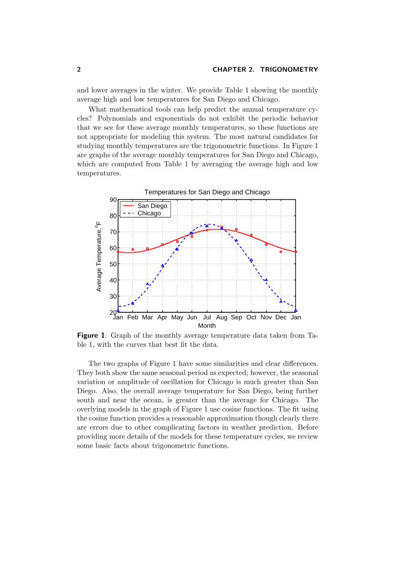
What mathematical tools can help predict the annual temperature cy-cles? Polynomials and exponentials do not exhibit the periodic behaviorthat we see for these average monthly temperatures, so these functions arenot appropriate for modeling this system. The most natural candidates forstudying monthly temperatures are the trigonometric functions. In Figure 1are graphs of the average monthly temperatures for San Diego and Chicago,which are computed from Table 1 by averaging the average high and lowtemperatures.
Jan Feb Mar Apr May Jun Jul Aug Sep Oct Nov Dec Jan20
30
40
50
60
70
80
90
Month
Ave
rage
Tem
pera
ture
, o F
Temperatures for San Diego and Chicago
San DiegoChicago
Figure 1: Graph of the monthly average temperature data taken from Ta-ble 1, with the curves that best fit the data.
The two graphs of Figure 1 have some similarities and clear differences.They both show the same seasonal period as expected; however, the seasonalvariation or amplitude of oscillation for Chicago is much greater than SanDiego. Also, the overall average temperature for San Diego, being furthersouth and near the ocean, is greater than the average for Chicago. Theoverlying models in the graph of Figure 1 use cosine functions. The fit usingthe cosine function provides a reasonable approximation though clearly thereare errors due to other complicating factors in weather prediction. Beforeproviding more details of the models for these temperature cycles, we reviewsome basic facts about trigonometric functions.

1. TRIGONOMETRIC FUNCTIONS 3
1.2 TRIGONOMETRIC FUNCTIONS
The trigonometric functions are often called circular functions, which em-phasizes their periodic nature and shows their connection to a circle. Let(x, y) be a point on a circle of radius r centered at the origin. Define theangle θ between the ray connecting the point to the origin and the x-axis.(See the diagram in Figure 2.)
(x,y)
r
θ
X
Y
Figure 2: Diagram of a circle on the Cartesian plane showing the relation-ship between trigonometric functions and the circle.
The six basic trigonometric functions are defined in termsof x, y, and r (including the sign of x and y) shown inthe diagram of Figure 2 by the following,
sin θ =y
r, cos θ =
x
r, tan θ =
y
x, (2.1)
csc θ =r
y, sec θ =
r
x, cot θ =
x
y. (2.2)
We will concentrate almost exclusively on the first two of these trigonometricfunctions, sine and cosine.

4 CHAPTER 2. TRIGONOMETRY
1.3 RADIAN MEASURE
Before discussing the nature of the trigonometric functions in more detail, weneed to discuss radian measure of the angle. If you have had trigonometrybefore, you probably used degrees to measure an angle. However, they arenot the appropriate unit to use in Calculus. The easiest way to considerradian measures is to examine the unit circle (which is simply the circle inthe diagram in Figure 2 with a radius of 1). From earlier courses, you mayrecall that the circumference of a circle is 2πr, so the distance around theperimeter of the unit circle is 2π. The radian measure of the angle θ in thediagram of Figure 2 is simply the distance along the circumference of theunit circle. Thus, a 45◦ angle is 1
8 of the distance around the unit circle or2π8 = π
4 radians. Similarly, 90◦ and 180◦ angles convert to π2 and π radians,
respectively.
The formulae for converting from degrees to radians orradians to degrees are,
1◦ =π
180= 0.01745 radians,
or,
1 radian =180◦
π≃ 57.296◦.
Trigonometric – Degree-Radian Conversion
This JavaScript is provided for easy conversions of degrees to radians orradians to degrees.
1.4 SINE AND COSINE
From the formulae for sine (sin) and cosine (cos) of Equation (2.1), we seethat if you take a unit circle, then the cosine function gives the x value ofthe angle (measured in radians), while the sine function gives the y valueof the angle. The tangent function (tan) gives the slope of the line (y/x).In Figure 3 we have a graph of the sine and cosine functions for the anglesfrom −2π to 2π, i.e., the graph shows sin(θ) and cos(θ) for θ ∈ [−2π, 2π].
There are several things to notice about these graphs. First, you noticethe 2π periodicity. In other words, the functions repeat the same patternevery 2π radians. This is clear from the circle of Figure 2 because everytime you go 2π radians around the circle, you return to the same point. The
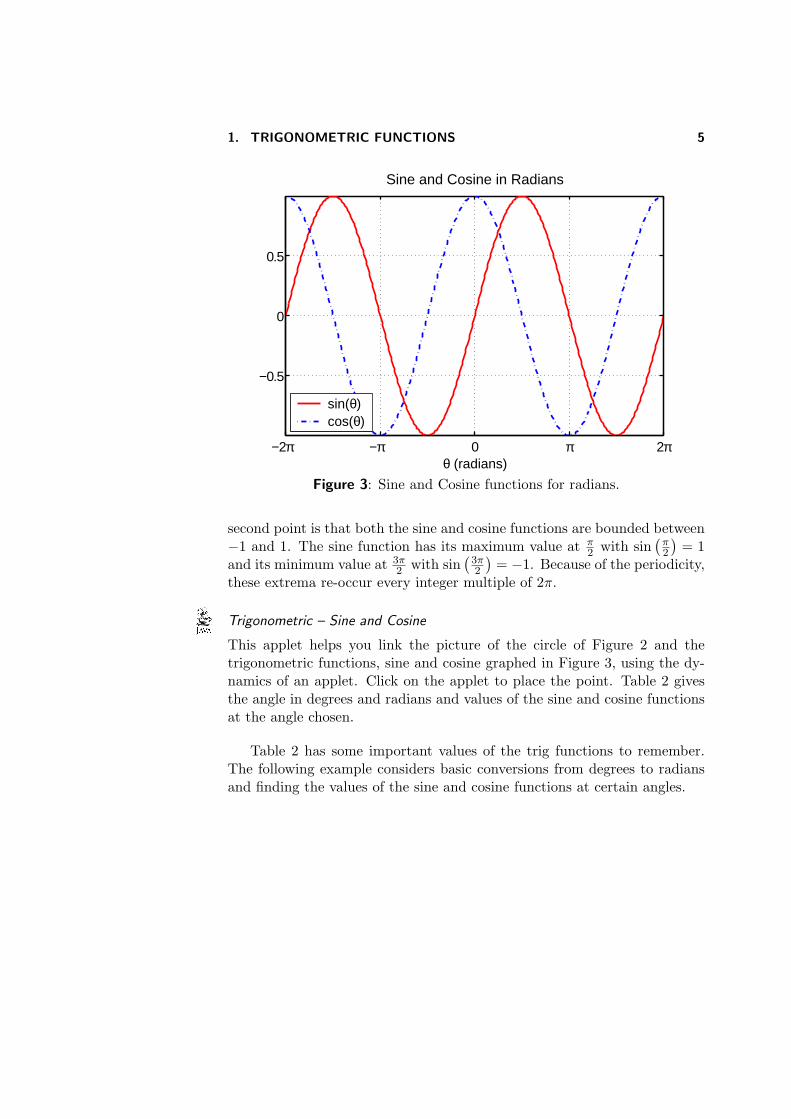
1. TRIGONOMETRIC FUNCTIONS 5
−2π −π 0 π 2π
−0.5
0
0.5
θ (radians)
Sine and Cosine in Radians
sin(θ)cos(θ)
Figure 3: Sine and Cosine functions for radians.
second point is that both the sine and cosine functions are bounded between−1 and 1. The sine function has its maximum value at π
2 with sin(π2
)= 1
and its minimum value at 3π2 with sin
(3π2
)= −1. Because of the periodicity,
these extrema re-occur every integer multiple of 2π.
Trigonometric – Sine and Cosine
This applet helps you link the picture of the circle of Figure 2 and thetrigonometric functions, sine and cosine graphed in Figure 3, using the dy-namics of an applet. Click on the applet to place the point. Table 2 givesthe angle in degrees and radians and values of the sine and cosine functionsat the angle chosen.
Table 2 has some important values of the trig functions to remember.The following example considers basic conversions from degrees to radiansand finding the values of the sine and cosine functions at certain angles.

6 CHAPTER 2. TRIGONOMETRY
θ sin(θ) cos(θ)
0 0 1π6
12
√32
π4
√22
√22
π3
√32
12
π2 1 0
π 0 −13π2 −1 0
2π 0 1
Table 2: Some of the most common values of trigonometric functions.
Example 1 Radians, Sine, and Cosine
Do not use a calculator for these.
a. Find the radian measure (x) for the following angles given in degrees,
θ = 0◦, 30◦, 90◦, 135◦, 210◦, 240◦, 270◦, 315◦. (2.3)
b. Determine the value of both sin(x) and cos(x) for each of these angles.
Solution: a. Recall the conversion formula in the main lecture section. Itstates that 1◦ = π/180 radians. Thus, given an angle in degrees θ the radianmeasure x is given by the formula
x =θπ
180.
The answers become fractional multiples of π. For example, when θ =135◦, then the radian measure is
x =135π
180=
3π
4.
The list of the angles in Equation (2.3) can be easily converted as shownin Section 1.3 to yield the following for all of the angles θ listed at (2.3),
x = 0,π
6,π
2,3π
4,7π
6,4π
3,3π
2, and
7π
4.
See Table 3 for a more complete listing.

1. TRIGONOMETRIC FUNCTIONS 7
b. To find the sine and cosine values for these angles without the use ofa calculator, we refer to Table 2 and use the geometry from the circle. If theangle is located in any quadrant other than the first quadrant, then we needto find the reference angle. The reference angle is an angle between 0 and π
2that is made with the x-axis, as we have θ in Figure 2. Then, for the angle7π6 that lies in the third quadrant, we find there is an angle of π
6 radiansbetween this ray and the negative side of the x-axis. Hence, consideringthat angle, we get a reference angle of π
6 radians. The reference angle thengives the magnitude of the sine and cosine functions, we just have to referto Table 2.
Lastly, we need to assign a sign to the function based on which quadrantit lies. Both sine and cosine are positive in the first quadrant. The sine ispositive and the cosine is negative in the second quadrant, while both arenegative in the third quadrant. In the fourth quadrant, the cosine is positiveand the sine is negative.
The angles that lie on either the x or y-axes are special ones that youshould get to know very well to make it much easier to sketch graphs ofthe trig functions. The angles x = 0, π
2 , and3π2 are special angles on the
axes, while the others (except x = π6 ) require finding the reference angle and
which quadrant they reside. We see that when x = 3π4 or 7π
4 , the referenceangle is π
4 , yielding the magnitude of both sine and cosine functions asfrom the table. However, the first of these is in the second quadrant, whilethe second is in the third quadrant. Since we discussed the angle 7π
6 , theremaining angle is x = 4π
3 . It has a reference angle of π3 and resides in the
third quadrant.In Table 3 we present a table summarizing our results. ▹
degrees (θ) 0◦ 30◦ 90◦ 135◦ 210◦ 240◦ 270◦ 315◦
radians (x) 0 π6
π2
3π4
7π6
4π3
3π2
7π4
sin(x) 0 12 1
√22 −1
2 −√32 −1 −
√22
cos(x) 1√32 0 −
√22 −
√32 −1
2 0√22
Table 3: Results of Example 1.
1.5 PROPERTIES AND IDENTITIES FOR SINE AND COSINE
There are a number of properties that are significant for sine and cosine.Below we list some of the most important properties for cosine.
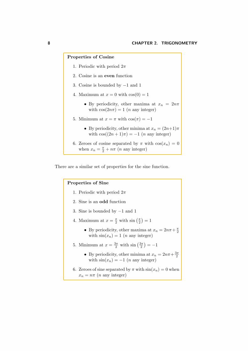
8 CHAPTER 2. TRIGONOMETRY
Properties of Cosine
1. Periodic with period 2π
2. Cosine is an even function
3. Cosine is bounded by −1 and 1
4. Maximum at x = 0 with cos(0) = 1
• By periodicity, other maxima at xn = 2nπwith cos(2nπ) = 1 (n any integer)
5. Minimum at x = π with cos(π) = −1
• By periodicity, other minima at xn = (2n+1)πwith cos((2n+ 1)π) = −1 (n any integer)
6. Zeroes of cosine separated by π with cos(xn) = 0when xn = π
2 + nπ (n any integer)
There are a similar set of properties for the sine function.
Properties of Sine
1. Periodic with period 2π
2. Sine is an odd function
3. Sine is bounded by −1 and 1
4. Maximum at x = π2 with sin
(π2
)= 1
• By periodicity, other maxima at xn = 2nπ+ π2
with sin(xn) = 1 (n any integer)
5. Minimum at x = 3π2 with sin
(3π2
)= −1
• By periodicity, other minima at xn = 2nπ+ 3π2
with sin(xn) = −1 (n any integer)
6. Zeroes of sine separated by π with sin(xn) = 0 whenxn = nπ (n any integer)

1. TRIGONOMETRIC FUNCTIONS 9
When studying trigonometry, there are many special trigonometric iden-tities that are frequently learned. We are going to highlight a very few thatare particularly useful.
Some Identities for Sine and Cosine
1. cos2(x) + sin2(x) = 1 for all values of x
2. Adding and subtracting angles for cosine
cos(x+ y) = cos(x) cos(y)− sin(x) sin(y)
cos(x− y) = cos(x) cos(y) + sin(x) sin(y)
3. Adding and subtracting angles for sine
sin(x+ y) = sin(x) cos(y) + cos(x) sin(y)
sin(x− y) = sin(x) cos(y)− cos(x) sin(y)
The first of these identities is readily verified using Pythagorean’s The-orem and the definitions of sine and cosine. The second two identities arenot as easily shown, and we will omit their proofs here2. The second twoidentities are useful in showing that from a modeling perspective, the sineand cosine functions are often interchangeable.
Example 2 Sine and Cosine Relationship
Use the trigonometric properties and identities to show that
cos(x) = sin(x+
π
2
)and
sin(x) = cos(x− π
2
)Solution: We begin using the additive identity formula for sine functions
sin(x+
π
2
)= sin(x) cos
(π2
)+ cos(x) sin
(π2
)2Proofs use basic definitions of the sine and cosine functions
http://en.wikipedia.org/wiki/Proofs of trigonometric identities#Angle sum identities -last visited 8/11
10 CHAPTER 2. TRIGONOMETRY
By our properties above, we know cos(π2
)= 0 and sin
(π2
)= 1, so
sin(x+
π
2
)= cos(x).
This relationship says that the cosine function is exactly the same as thesine function, but shifted out of phase by −π
2 (or the sine curve shifted tothe left by π
2 ).
Using the subtractive identity formula for cosine functions
cos(x− π
2
)= cos(x) cos
(π2
)+ sin(x) sin
(π2
)Again cos
(π2
)= 0 and sin
(π2
)= 1, so
cos(x− π
2
)= sin(x).
This relationship shows that the sine function has the same form as thecosine function, but shifted out of phase by π
2 (or the cosine curve shiftedto the right by π
2 ). ▹
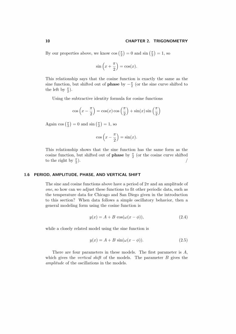
1.6 PERIOD, AMPLITUDE, PHASE, AND VERTICAL SHIFT
The sine and cosine functions above have a period of 2π and an amplitude ofone, so how can we adjust these functions to fit other periodic data, such asthe temperature data for Chicago and San Diego given in the introductionto this section? When data follows a simple oscillatory behavior, then ageneral modeling form using the cosine function is
y(x) = A+B cos(ω(x− ϕ)), (2.4)
while a closely related model using the sine function is
y(x) = A+B sin(ω(x− ϕ)). (2.5)
There are four parameters in these models. The first parameter is A,which gives the vertical shift of the models. The parameter B gives theamplitude of the oscillations in the models.

1. TRIGONOMETRIC FUNCTIONS 11
Trigonometric Model ParametersVertical Shift and Amplitude
• The model parameter A is the vertical shift, whichis associated with the average height of the model
• The model parameter B gives the amplitude, whichmeasures the distance from the average, A, to themaximum (or minimum) of the model
The parameter ω is the frequency of the models.
Trigonometric Model ParametersFrequency and Period
• The model parameter ω is the frequency, whichgives the number of periods of the model that occuras x varies over 2π radians
• The period is given by T =2π
ω
It is the periodic nature of the models for which these functions have beenchosen. The last parameter, ϕ, is the phase shift .
Trigonometric Model ParametersPhase Shift
• The model parameter ϕ is the phase shift, whichshifts our models to the left or right, thus, gives ahorizontal shift
• If the period is denoted T = 2πω , then the principle
phase shift satisfies ϕ ∈ [0, T )
• By periodicity of the model, if ϕ is any phase shift,then
ϕ1 = ϕ+ nT = ϕ+2nπ
ω, n an integer
is a phase shift for an equivalent model

12 CHAPTER 2. TRIGONOMETRY
When fitting the cosine and sine models, (2.4) and (2.5), there are choicesthat can be made with the parameters. The parameter, A, is unique. Theparameters for amplitude and frequency, B and ω, are unique in magnitude,but the sign of the parameter can be chosen by the modeler. Usually, weprefer to take the parameters B and ω to be positive. Because of the peri-odicity of these trigonometric functions, there are infinitely many possiblechoices for the phase shift, ϕ. However, it is customary to select the phaseshift satisfying 0 ≤ ϕ < T , the principle phase shift . By taking the principlephase shift and positive values for the amplitude and frequency, then thefour parameters in the cosine and sine models, A, B, ω, and ϕ, are unique.
Example 3 Period and Amplitude for the Sine Function
This first example examines amplitude and frequency in the sine model.Find the period and amplitude of
y(x) = 4 sin(2x).
Determine all maxima and minima for x ∈ [−2π, 2π] and sketch the graph.
Solution: From the information above, we see that the amplitude of thisfunction is 4, which says that it oscillates between −4 and 4, and the fre-quency is 2. The easiest way to find the period T is to let x = T in thefunction, then set the argument of the trig function to 2π, and finally solvethis for T . This means,
2T = 2π, so T = π.
Alternately, the definition of period given the frequency, ω, gives:
T =2π
ω=
2π
2= π.
From Table 2, we see that this function begins at 0 when x = 0. Itachieves a maximum of 4 where the argument 2x = π
2 , which gives x = π4 .
The function decreases to a minimum of −4 at x = 3π4 , since the argument
there is 2x = 3π2 . Then it increases to where it completes its cycle at x = π.
By periodicity, there are other maxima at x = π + π4 = 5π
4 , x = −π + π4 =
−3π4 , and x = −9π
4 . Similarly, there are other minima at x = −5π4 ,−
π4 , and
7π4 .
The sine function is an odd function, so the graph is symmetric aboutthe origin. The graph is shown in Figure 4 for x ∈ [−2π, 2π]. ▹

1. TRIGONOMETRIC FUNCTIONS 13
−2π −π 0 π 2π
−3
−2
−1
0
1
2
3
x (radians)
y
y = 4 sin(2x)
Figure 4: Graph of the function y = 4 sin(2x) of Example 3.
Example 4 Graphing a Sine Function
Sketch the graph of the following function,
y(x) = 3 sin(2x)− 2,
for −2π ≤ x ≤ 2π. Determine the amplitude and period of oscillation forthis function. Find all maxima and minima.
Solution: From above, this function is shifted vertically downward by theconstant −2. The amplitude is given by 3 (multiplying the sine function),so the graph will oscillate between −5 ≤ y ≤ 1. These high and low pointsof the graph are found by letting the sine function take its maximum andminimum values given by 1 and −1, respectively. According to Table 2,this happens when the argument 2x = π
2 , which implies x = π4 . Then
sin(2x) = sin(π/2) = 1. Thus, at x = π4 ,
y(π/4) = 3(1)− 2 = 1.
When 2x = 3π2 , or x = 3π
4 , then sin(2x) = sin(3π/2) = −1. Thus, atx = 3π/4 we have,
y(3π/4) = 3(−1)− 2 = −5.

14 CHAPTER 2. TRIGONOMETRY
To find the period, T , we have
T =2π
ω, so T =
2π
2= π.
Thus, the period of this function is π.The best way to sketch a graph of either the sine and cosine function
is to take the period of the function, then divide it into 4 even parts. Forthis example, we divide the interval [0, π] into 4 parts. Next we evaluate thefunction at each of the endpoints of these subintervals, which for this caseoccurs at 0, π/4, π/2, 3π/4, and π. We obtain the following,
y(0) = 3 sin(2(0))− 2 = 3 sin(0)− 2 = −2,
y(π/4) = 3 sin(2(π/4))− 2 = 3 sin(π/2)− 2 = 1,
y(π/2) = 3 sin(2(π/2))− 2 = 3 sin(π)− 2 = −2,
y(3π/4) = 3 sin(2(3π/4))− 2 = 3 sin(3π/2)− 2 = −5,
y(π) = 3 sin(2(π))− 2 = 3 sin(2π)− 2 = −2.
−2π −π 0 π 2π
−4
−3
−2
−1
0
x (radians)
y
y = 3 sin(2x) − 2
Figure 5: Graph of the function y(x) = 3 sin(2x)− 2 of Example 4.
This takes on the important values (minima and maxima) and goesthrough one cycle, which makes the sketching easy. One simply repeatsthe graph to extend it. In Figure 5 there is a graph of this function.

1. TRIGONOMETRIC FUNCTIONS 15
Since this function is periodic with period π and a maximum of y = 1occurs at x = π
4 , there are the other maxima at x = π4 − 2π = −7π
4 ,π4 − π = −3π
4 , and π4 + π = 5π
4 . Since a minimum of y = −5 occurs atx = 3π
4 , we can add and subtract integer multiples of π to obtain the otherminima at x = −5π
4 , −π4 , and
7π4 . ▹
Example 5 Vertical Shift with the Cosine Function
Consider a model given by
y(x) = 3− 2 cos(3x), x ∈ [0, 2π].
Find the vertical shift, period, and amplitude of this model. Determine allminima and maxima in the domain and sketch the graph.
Solution: This function is shifted vertically by the constant 3. The ampli-tude is the 2 multiplying the cosine function, but there is a negative sign inthis model, which forces the model in the opposite direction of the cosinemodel given by (2.4). The vertical shift of 3 and amplitude of 2 means thatthe graph oscillates between 1 ≤ y ≤ 5, since the range of the cosine functionvaries between −1 and 1.
To find the period, T , we solve
3T = 2π, so T =2π
3.
Thus, the period of this function is 2π3 .
The easiest way to find a minimum or maximum is to use the largestand smallest values of the cosine function, 1 and −1, which occur when theargument is 0 and π, see Table 2. Hence, when x = 0, cos(3x) = 1 and
y(0) = 3− 2(1) = 1,
which is a minimum. When x = π3 , cos(3x) = cos(π) = −1 and
y(π/3) = 3− 2(−1) = 5,
which is a maximum. By periodicity, the other minima occur at integermultiples of 2π
3 , which gives the minima in the domain at x = 0, 2π3 , 4π
3 ,and 2π. Similarly, the maxima in the domain occur at x = π
3 , π, and5π3 .
Figure 6 is a graph of this function.

16 CHAPTER 2. TRIGONOMETRY
0 π/2 π 3π/2 2π1
2
3
4
x (radians)
yy = 3 − 2 cos(3x)
Figure 6: Graph of the function y = 3− 2 cos(3x) of Example 5.
We can insert a phase shift of half a period to make the constant forthe amplitude be positive and produce the same model. Consider the modelwith a half period phase shift given by
y(x) = 3 + 2 cos(3(x− π
3 )).
To show this is the same model we employ the angle subtraction identityfor the cosine function.
y(x) = 3 + 2 cos(3(x− π
3 )),
= 3 + 2 cos(3x− π),
= 3 + 2(cos(3x) cos(π) + sin(3x) sin(π)),
= 3− 2 cos(3x),
since cos(π) = −1 and sin(π) = 0. ▹
Phase Shift of Half a Period
A phase shift of half a period creates an equivalent sineor cosine model with the sign of the amplitude reversed.

1. TRIGONOMETRIC FUNCTIONS 17
Phase shifts are important matching data in periodic models. The easiestmodel to match a phase shift is the cosine model (2.4), since the maximumof the cosine function occurs when the argument is zero. The next exam-ple explores graphing the cosine model with a phase shift and gives thecorresponding sine model that produces the same graph.
Example 6 Graphing a Cosine Function with a Phase Shift
Consider the following cosine model, which includes a phase shift
y(x) = 4 + 6 cos
(x− π
2
), x ∈ [−4π, 4π].
Find the vertical shift, amplitude, period, and phase shift for this model. De-termine all maxima and minima in the domain. Finally, find the equivalentsine model with the principle phase shift (a phase shift, ϕ ∈ [0, T ), where Tis the period of the model.
Solution: From the form of the model it is easy to read off the vertical shift,given by A = 4. The amplitude is similarly easy to read as B = 6. If werewrite the function as,
y(x) = 4 + 6 cos(12(x− π)
),
then the frequency of the model is ω = 12 . This allows computation of the
period, T ,
T =2π12
= 4π.
This also allows easy reading of the phase shift, ϕ = π.The phase shift indicates that this is a cosine function shifted horizontally
x = π units to the right. Since the cosine function has a maximum valuewhen its argument is zero (see Table 2), this model will achieve a maximumat x = π. With the period being T = 4π, the easiest way to graph thisfunction is to start at x = π and proceed to x = 5π, completing one period.Then we use the periodicity to get the desired graph over the domain.
The significant points for evaluation are always each quarter of the pe-riod. Thus, for this model the points of interest will be x = π, 2π, 3π, 4π,and 5π. (Note that the last point is outside the domain.) We substitute
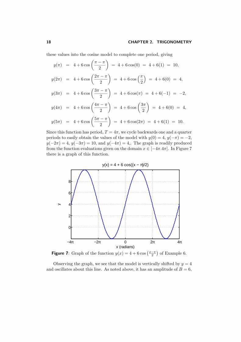
18 CHAPTER 2. TRIGONOMETRY
these values into the cosine model to complete one period, giving
y(π) = 4 + 6 cos
(π − π
2
)= 4 + 6 cos(0) = 4 + 6(1) = 10,
y(2π) = 4 + 6 cos
(2π − π
2
)= 4 + 6 cos
(π2
)= 4 + 6(0) = 4,
y(3π) = 4 + 6 cos
(3π − π
2
)= 4 + 6 cos(π) = 4 + 6(−1) = −2,
y(4π) = 4 + 6 cos
(4π − π
2
)= 4 + 6 cos
(3π
2
)= 4 + 6(0) = 4,
y(5π) = 4 + 6 cos
(5π − π
2
)= 4 + 6 cos(2π) = 4 + 6(1) = 10.
Since this function has period, T = 4π, we cycle backwards one and a quarterperiods to easily obtain the values of the model with y(0) = 4, y(−π) = −2,y(−2π) = 4, y(−3π) = 10, and y(−4π) = 4,. The graph is readily producedfrom the function evaluations given on the domain x ∈ [−4π.4π]. In Figure 7there is a graph of this function.
−4π −2π 0 2π 4π
0
2
4
6
8
x (radians)
y
y(x) = 4 + 6 cos((x − π)/2)
Figure 7: Graph of the function y(x) = 4 + 6 cos(x−π2
)of Example 6.
Observing the graph, we see that the model is vertically shifted by y = 4and oscillates about this line. As noted above, it has an amplitude of B = 6,

1. TRIGONOMETRIC FUNCTIONS 19
so oscillates 6 units above and below this average line with a period ofT = 4π. Finally, we note that this cosine function is shifted to the right bythe phase shift, ϕ = π.
From either the graph or the values computed above, we see that in thedomain, this model has maxima of y(xmax) = 10 at xmax = −3π and π.The model has minima of y(xmin) = −2 at xmin = −π and 3π.
A closer look at the graph in Figure 7 indicates that this model looksmore like a standard sine function model. Suppose we want to use the sinemodel
y(x) = A+B sin(ω(x− ϕ)).
Since we want the graph to be identical, the vertical shift, amplitude, andperiod must be the same, so A = 4, B = 6, and ω = 1
2 or
y(x) = 4 + 6 sin(12(x− ϕ)
).
It remains to find the appropriate phase shift, ϕ.Recall from Example 2 that the cosine function is horizontally shifted to
the left by π2 of the sine function. Thus,
cos(12(x− π)
)= sin
(12(x− π) + π
2
)= sin
(12(x− ϕ)
).
It follows that we want
−π2+π
2= −ϕ
2or ϕ = 0.
Thus, there is no phase shift for the sine model, and the equivalent sinemodel is given by
y(x) = 4 + 6 sin(x2
).
▹
The example above shows that models using sine or cosine functionsare equivalent when the vertical shift, amplitude, and period are the same.Only the phase shift differs, and our trigonometric identities readily find thisdifference in the phase shift.
20 CHAPTER 2. TRIGONOMETRY
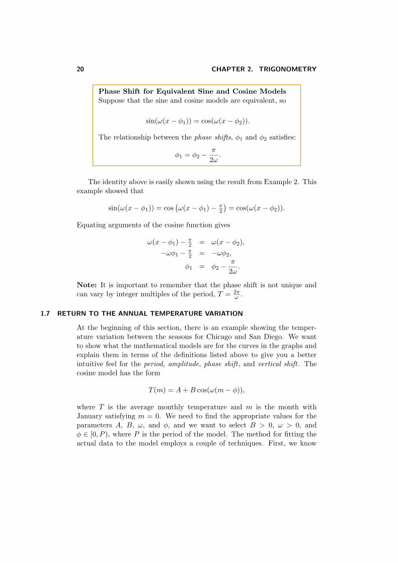
Phase Shift for Equivalent Sine and Cosine ModelsSuppose that the sine and cosine models are equivalent, so
sin(ω(x− ϕ1)) = cos(ω(x− ϕ2)).
The relationship between the phase shifts, ϕ1 and ϕ2 satisfies:
ϕ1 = ϕ2 −π
2ω.
The identity above is easily shown using the result from Example 2. Thisexample showed that
sin(ω(x− ϕ1)) = cos(ω(x− ϕ1)− π
2
)= cos(ω(x− ϕ2)).
Equating arguments of the cosine function gives
ω(x− ϕ1)− π2 = ω(x− ϕ2),
−ωϕ1 − π2 = −ωϕ2,
ϕ1 = ϕ2 −π
2ω.
Note: It is important to remember that the phase shift is not unique andcan vary by integer multiples of the period, T = 2π
ω .
1.7 RETURN TO THE ANNUAL TEMPERATURE VARIATION
At the beginning of this section, there is an example showing the temper-ature variation between the seasons for Chicago and San Diego. We wantto show what the mathematical models are for the curves in the graphs andexplain them in terms of the definitions listed above to give you a betterintuitive feel for the period, amplitude, phase shift , and vertical shift . Thecosine model has the form
T (m) = A+B cos(ω(m− ϕ)),
where T is the average monthly temperature and m is the month withJanuary satisfying m = 0. We need to find the appropriate values for theparameters A, B, ω, and ϕ, and we want to select B > 0, ω > 0, andϕ ∈ [0, P ), where P is the period of the model. The method for fitting theactual data to the model employs a couple of techniques. First, we know

1. TRIGONOMETRIC FUNCTIONS 21
that the period of this function must be 12 months. This constrains ourparameter ω to satisfy
12ω = 2π or ω =π
6= 0.5236.
We know that the cosine function oscillates around its average, so thevalue of A, which gives the vertical shift, is the average of the monthly tem-peratures. From Table 1, we find the average temperature of San Diegofor each month by averaging the minimum and maximum temperaturesrecorded each month. The average temperature for the year satisfies:
A = 57.5+59+59.5+62+64+67+71+72.5+71.5+68+62+57.512
= 64.29,
while for Chicago, we findA = 49.17.
There are a several methods to obtain fits for the parameters B andϕ. We chose to find a nonlinear least squares fit to these parameters withExcel’s Solver. The model for the average monthly temperature in San Diegois given by
T (m) = 64.29 + 7.29 cos(0.5236(m− 6.74)),
while the average monthly temperature in Chicago follows the formula
T (m) = 49.17 + 25.51 cos(0.5236(m− 6.15)).
Here, we have again that T is the average monthly temperature and m isthe month number with January satisfying m = 0.
We have discussed the vertical shift (average temperature given by A)and the period (12 months giving a frequency of ω = π
6 = 0.5236). The am-plitude is given by the parameter B, which represents the maximum amountthe temperature varies from the annual average. With its “Mediterranean”climate, San Diego has the significantly lower amplitude with only a 7.29◦Fvariation higher and lower than its average annual temperature. Chicagohas a temperature variation of 25.51◦F above and below its lower average of49.17◦F. Thus, our model predicts that the temperature of San Diego willvary from 57.0◦F to 71.58◦F (average monthly temperature), while Chicagowill vary from 23.66◦F to 74.68◦F (average monthly temperature). Theseshould be apparent from the graph of Figure 1.
Finally, we interpret the phase shift, ϕ, which indicates that the graph isshifted ϕ units to the right. For San Diego, we see a phase shift of ϕ = 6.74.

22 CHAPTER 2. TRIGONOMETRY
This means that the maximum temperature occurs at 6.74 months (lateJuly), instead of January, as one would expect. For Chicago, the phase shiftis ϕ = 6.15 months, which gives the high occurring a little earlier (earlyJuly). Be sure to view the original graph of Figure 1, and match how theparameters are reflected in this graph as it is important for understandingthe use of trigonometric functions.
The cosine models given above for the average temperature of San Diegoand Chicago can be rewritten with the sine function,
T (m) = A+B sin(ω(m− ϕ2)).
The values for A, B, and ω are the same for both the sine and cosine models.However, the phase shift for the sine model differs from the cosine model.The formula above shows that the sine phase shift, ϕ2, satisfies
ϕ2 = ϕ− π
2ω,
where ϕ is the phase shift from the cosine model. This formula gives ϕ2 =3.74 for San Diego and ϕ2 = 3.15 for Chicago. This phase shift for thesine model is a quarter of the period less than the phase shift for the cosinemodel. Thus, we write the sine models for the average monthly temperaturein San Diego,
T (m) = 64.29 + 7.29 sin(0.5236(m− 3.74)),
and the average monthly temperature in Chicago,
T (m) = 49.17 + 25.51 sin(0.5236(m− 3.15)).
These models produce exactly the same graphs as seen in Figure 1.
Example 7 Model with Phase Shift
Consider an oscillatory set of population data that is periodic with a periodof 10 yr. Suppose that there is a maximum population (in thousands) of 26at t = 2 and a minimum population (in thousands) of 14 at t = 7. Assumethese data fit a model of the form
y(t) = A+B sin(ω(t− ϕ)).
Find the appropriate constants A, B, ω, and ϕ. Choose B > 0 and ω > 0,then find ϕ ∈ [0, 10). Since ϕ is not unique, find values of ϕ with ϕ ∈ [−10, 0)

1. TRIGONOMETRIC FUNCTIONS 23
and ϕ ∈ [10, 20). Graph the model. In addition, repeat this process for thecosine model
y(t) = A+B cos(ω(t− ϕ2)).
Solution: The vertical shift, A, is the average of the high and low points ofthe data, so
A = 26+142 = 20.
The amplitude, B, is the distance from the maximum to the average, so
B = 26− 20 = 6.
Since the period is T = 10 years, the frequency, ω, satisfies
ω = 2π10 = π
5 .
Note that the times of the maximum and minimum are separated by half aperiod. This will always be the case of our sine and cosine models.
We are given that the maximum of 26 occurs at t = 2, so the modelsatisfies:
y(2) = 26 = 20 + 6 sin(π5 (2− ϕ)
).
From this equation it is clear that
sin(π5 (2− ϕ)
)= 1.
Recall that the sine function is at its maximum with value one when itsargument is π
2 , so
π
5(2− ϕ) = π
2 ,
2− ϕ = 52 ,
ϕ = −12 .
This value of ϕ is not in the interval [0, 10), but the periodicity, T = 10, ofthe model is also reflected in the phase shift, ϕ. We can write
ϕ = −12 + 10n, n an integer
ϕ = ...− 10.5,−0.5, 9.5, 19.5, ...
with the principle phase shift being ϕ = 9.5. It follows that we can writethe sine model
y(t) = 20 + 6 sin(π5 (t− 9.5)
),

24 CHAPTER 2. TRIGONOMETRY
−10 −5 0 5 1010
15
20
25
30
t (years)
yy(t) = 20 + 6 sin(π(t − 9.5)/5)
Figure 8: Graph of the model y(t) = 20 + 6 sin(π(t− 9.5)/5) of Example 7.
and its graph is given in Figure 8. From the formula for ϕ, we could alsouse phase shifts of ϕ = −1
2 or ϕ = 19.5.The cosine model has the form
y(t) = 20 + 6 cos(π5 (t− ϕ2)
),
where the vertical shift, amplitude, and frequency match the sine model. Itremains to find the phase shift, ϕ2. The maximum of the cosine functionoccurs when its argument is 0, so
π
5(2− ϕ2) = 0,
ϕ2 = 2.
It follows that the cosine model satisfies
y(t) = 20 + 6 cos(π5 (t− 2)
).
By periodicity of the phase shift, we have
ϕ2 = 2 + 10n, n an integer
ϕ2 = ...− 8, 2, 12, 22, ...,
where the principle phase shift is ϕ2 = 2. ▹

1. TRIGONOMETRIC FUNCTIONS 25
1.8 BODY TEMPERATURE
Humans, like many organisms, undergo circadian rhythms for many of theirbodily functions. Circadian rhythms are the daily fluctuations that aredriven by the light/dark cycle of the Earth, which seems to affect the pinealgland in the head. The average body temperature for a human is about37◦C. However, this temperature normally varies a few tenths of a degree ineach individual with distinct regularity. The body is usually at its hottestaround 10 or 11 AM and at its coolest in the late evening, which helpsencourage sleep.
Suppose that measurements on a particular individual show that he hasa high body temperature of 37.1◦C at 10 am. He has a low body temperatureof 36.7◦C at 10 pm. Assume that his body temperature, T (t), satisfies thefollowing equation,
T (t) = A+B cos(ω(t− ϕ)), (2.6)
for some parameters A, B, ω, and ϕ. Use the data above to find the fourparameters with B > 0, ω > 0, and ϕ ∈ [0, 24). We show how to selectreasonable parameter values for this cosine model. We also create the sinemodel.
Solution: In this problem, we know that one day is 24 hours, so the periodof the function is 24. (Be careful not to confuse the temperature T (t) withour previous notation of T as the period.) The frequency is given by
ω =2π
24=
π
12.
As seen in our examples above, the parameter A represents the aver-age temperature of the body. The mean (average) temperature is half-waybetween the extreme values, so
A =37.1◦C+ 36.7◦C
2= 36.9◦C.
The difference between the maximum and the average temperature givesthe amplitude of variation in the body temperature. We can see that thedifference from the mean to the maximum (or the minimum) is 0.2◦C, whichis the amplitude of this trigonometric model, B.
Last, the phase will determine at what time the highest point occurs.The cosine function has its maximum when its argument is 0 (or any integermultiple of 2π). Since the highest body temperature occurs at t = 10, wefind the appropriate phase shift by solving
ω(10− ϕ) = 0 or ϕ = 10.

26 CHAPTER 2. TRIGONOMETRY
0 5 10 15 20
36.75
36.8
36.85
36.9
36.95
37
37.05
t (hours)
Tem
pera
ture
(o C)
Body Temperature
Figure 9: Graph of the body temperature.
It follows that the phase shift is given by ϕ = 10.Using these values for the parameters in the Equation (2.6) results in an
equation modeling the temperature of the body at a given time,
T (t) = 36.9 + 0.2 cos(π12(t− 10)
),
which is shown graphically in Figure 9. We see from the graph of Figure 9that the maximum is 37.1◦C, and it is shifted to 10 AM, a time when mostof us are becoming active. The minimum occurs at 10 PM. A tendencyof this minimum to be delayed in adolescence can result in sleep disorders,abnormal sleep patterns, and chronic sleep deprivation.
If the body temperature is modeled by a sine function of the form
T (t) = A+B sin(ω(t− ϕ2)),
then the parameters A = 36.9, B = 0.2, and ω = π12 , the same as for the
cosine model. It only remains to find the phase shift, ϕ2. As seen before,the phase shift for the sine model is a quarter period less than the one forthe cosine model. From our formula above,
ϕ2 = 10− π
2ω= 10− 6 = 4.
Thus, the equivalent sine model is given by
T (t) = 36.9 + 0.2 sin(π12(t− 4)
).

1. TRIGONOMETRIC FUNCTIONS 27
1.9 EXERCISES
1. Complete the following table. Do NOT use a calculator! When the valuefor the sine or cosine function is given, state all possible solutions for theangles with 0 ≤ x ≤ 2π or 0 ≤ θ ≤ 360◦.
radian (x) degree (θ) sin(x) cos(x)3π4
−12
330◦
−√32
10π3
√22
210◦
−1
−5π4
0
270◦
−12
Sketch a graph of the following trigonometric functions for −2π ≤ x ≤ 2π.Give the period of the function.
2. y(x) = 3 cos(2x) 3. y(x) = 2− 4 sin(3x)
4. y(x) = 1 + 3 cos(2x) 5. y(x) = 4 sin(x2
)6. y(x) = 2 sin(4x) + 1 7. y(x) = 5− 2 cos
(x2
)8. y(x) = 2− cos(2(x− π)) 9. y(x) = 2 sin
(3(x+ π
2
))10. For each of the following problems (see 7 and 8 above) find an equivalentmodel of the form
y(x) = A+B cos(ω(x− ϕ)),
where the amplitude, B > 0, and the principle phase shift, ϕ ∈ [0, T ) withT being the period of the function.
a. y(x) = 5− 2 cos(x2
)b. y(x) = 2− cos(2(x− π))

28 CHAPTER 2. TRIGONOMETRY
11. For each of the following problems (see 3 and 9 above) find an equivalentmodel of the form
y(x) = A+B sin(ω(x− ϕ)),
where the amplitude, B > 0, and the principle phase shift, ϕ ∈ [0, T ) withT being the period of the function.
a. y(x) = 2− 4 sin(3x) b. y(x) = 2 sin(3(x+ π
2
))12. The lungs do not completely empty or completely fill in normal breath-ing. The volume of the lungs normally varies between 2200 ml and 2800 mlwith a breathing rate of 24 breaths/min. This exchange of air is called thetidal volume. One approximation for the volume of air in the lungs uses thecosine function written in the following manner,
V (t) = A+B cos(ωt),
where A, B, and ω are constants and t is in minutes. Use the data above tocreate a model, i.e., find A, B, and ω that simulates the normal breathing ofan individual for one minute. Graph the function for 10 sec., clearly showingthe maximum and minimum volumes, and frequency of inhalation.
13. a. The heart pumps blood at a regular rate of about 60 pulses per minute.The heart volume is about 140 ml, and it pushes out about 1/2 its volume(70 ml) with each beat. Use a model of the following form to simulate thevolume of blood, B(t), in the heart at any time t,
B(t) = a+ b sin(ωt),
where a, b, and ω are constants and t is in minutes. Sketch a graph of thisfunction for 5 sec., clearly showing the maximum and minimum volumes,and frequency of the beating heart.
b. When the heart pushes out blood, the pressure, P (t), in the aortaand arterioles increases to 120 mm Hg. When the heart fills with blood, thepressure falls to about 80 mm Hg. Use a similar model of the form
P (t) = c+ d sin(ωt),
where c, d, and ω are constants with d and ω positive and t is in minutes.Again you sketch a graph of this function for 5 sec., clearly showing themaximum and minimum volumes, and frequency of the beating heart.

1. TRIGONOMETRIC FUNCTIONS 29
c. Consider your answer in Part b, and determine an equivalent modelof the form
P (t) = C +D cos(ν(t− ϕ)),
where D > 0, ν > 0, and ϕ ∈ [0, T ) with T being the period of the heart.Relate your constants in this model to the one in Part b.
14. The average body temperature for a human is about 37◦C. However, thistemperature normally varies a few tenths of a degree in each individual withdistinct regularity. The body is usually at its hottest around 10 or 11 amand at its coolest in the late evening, which helps encourage sleep. Whenan individual switches to night shift work, his body temperature cycle hasto switch also.
a. Suppose that a worker on the night shift finds his hottest body tem-perature to be at 2 am with a body temperature of 37.1◦C, then 12 hourslater his body temperature achieves a minimum of 36.7◦C. Assume that thebody temperature can be modeled using a trigonometric function and isgiven by
T (t) = A+B cos(ω(t− ϕ)),
where A, B > 0, ω > 0, and ϕ ∈ [0, 24) are constants and t is in hours.Use the data above to find the four parameters, then sketch a graph for thetemperature of this individual for one day.
b. Determine an equivalent temperature model of the form
T (t) = C +D sin(ν(t− ψ)),
where D > 0, ν > 0, and ψ ∈ [0, 24). Relate your constants in this modelto the one above. Also, find a value of the phase shift ψ ∈ [−24, 0), whichproduces an equivalent model.
15. a. Iguanas are cold-blooded or ectothermic organisms with their bodytemperature depending on the external temperature. (See www.anapsid.orgfor more information.) Their natural habitat lies near the equator, wherethe sun shines about 12 hours a day. The iguana’s temperature cycles duringthe day, with a low of 75◦F at about 3 am and a high of 104◦F at about3 pm. Assume that the body temperature of an iguana can be modeledusing the following function,
T (t) = A+B sin(ω(t− ϕ)),
where A, B, ω, and ϕ are constants and t is in hours. Use the data aboveto find the four parameters, then sketch a graph for the temperature of atypical iguana for one day.
30 CHAPTER 2. TRIGONOMETRY
b. A temperature of 88◦F for at least 12 hours a day is critical for thehealth of an iguana. About how many hours a day does your iguana modelgive this temperature? (Use the graph which you have created to make areasonable estimate.)
c. Determine an equivalent temperature model of the form
T (t) = C +D cos(ν(t− ψ)),
where D > 0, ν > 0, and ψ ∈ [0, 24). Relate your constants in this modelto the one above. Also, find a value of the phase shift ψ ∈ [−24, 0), whichproduces an equivalent model.
16. During the human female menstrual cycle, the gonadotropin, FSH orfollicle stimulating hormone, is released from the pituitary in a sinusoidalmanner with a period of approximately 28 days. Guyton’s text on MedicalPhysiology [1] shows that if we define day 0 (t = 0) as the beginning ofmenstruation, then FSH, F (t), cycles with a high concentration of about 4(“relative units”) around day 9 and a low concentration of about 1.5 aroundday 23.
a. Consider a model of the concentration FSH (in “relative units”) givenby,
F (t) = A+B cos(ω(t− ϕ)),
where A, B, ω, and ϕ are constants and t is in days. Use the data aboveto find the four parameters, then sketch a graph for the concentration ofFSH over one period. If ovulation occurs around day 14, then what is theapproximate concentration of FSH at that time?
b. Determine an equivalent FSH model of the form
F (t) = C +D sin(ν(t− ψ)),
where D > 0, ν > 0, and ψ ∈ [0, 28). Relate your constants in this modelto the one above. Also, find a value of the phase shift ψ ∈ [28, 56), whichproduces an equivalent model.
1.10 REFERENCES
[1] A. C. Guyton and J. E. Hall, Textbook of Medical Physiology, 9thedition, Philadelphia, W. B. Saunders (1996).
[2] J. M. Mahaffy and A. Chavez-Ross, Calculus: A Mathematical Ap-proach for the Life Sciences, Volume I, San Diego State University,Pearson Custom Publishing (2009).