EENS 2120 PetrologyProf. Stephen A. Nelson Tulane University

Triangular Plots in Metamorphic PetrologyThis document last updated on 10­Mar­2011

Like igneous rocks, most metamorphic rocks are composed of 9 or more major elements.  Thus,initially it would appear that we are dealing with a 9 or 10 component system.  Recall, however,that the number of components in any given system is the minimum number required to definethe composition of all phases in the system.  Thus, since constituents like Na2O and K2O are notusually found as separate mineral phases, we can combine these with other constituents, likeAl2O3 and SiO2 in the feldspars, and thus reduce the number of components required to defineour system.

This is especially important if we wish to graphically display chemical rock and mineral data in away that is easily visualized.  In fact, the best way to visualize such data is to attempt to reducethe number of components to 3, so that we can plot the compositions of rocks and minerals on atriangular composition diagram.  Before discussing how this is done, we first review some of theprinciples of three component compositional diagrams. 

General Three Component Compositional Diagrams

For the moment we will assume that we are in a true 3 component system and the minerals thatwe display on a triangular composition diagram is a set of mineral that are in equilibrium over anarrow range of temperature and pressure.  

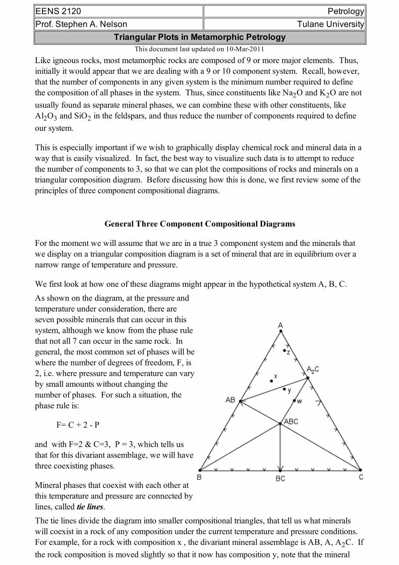
We first look at how one of these diagrams might appear in the hypothetical system A, B, C. As shown on the diagram, at the pressure andtemperature under consideration, there areseven possible minerals that can occur in thissystem, although we know from the phase rulethat not all 7 can occur in the same rock.  Ingeneral, the most common set of phases will bewhere the number of degrees of freedom, F, is2, i.e. where pressure and temperature can varyby small amounts without changing thenumber of phases.  For such a situation, thephase rule is:

F= C + 2 ­ P 

and  with F=2 & C=3,  P = 3, which tells usthat for this divariant assemblage, we will havethree coexisting phases.

Mineral phases that coexist with each other atthis temperature and pressure are connected bylines, called tie lines.  The tie lines divide the diagram into smaller compositional triangles, that tell us what mineralswill coexist in a rock of any composition under the current temperature and pressure conditions. For example, for a rock with composition x , the divariant mineral assemblage is AB, A, A2C.  Ifthe rock composition is moved slightly so that it now has composition y, note that the mineral

assemblage will change to AB, A2C, ABC. 

Within each compositional triangle, we can use the lever rule to estimate the proportions of thephases that will occur in the rock.  For example, a rock with composition x will have the samemineral assemblage as a rock with composition z, but rock z will have a much higher proportionof the mineral A.

In a rare case, note that it is possible for a rock composition to lie exactly on a tie line, forexample the rock with composition w.  Such a rock would consist of approximately equalproportions of the minerals ABC and A2C.  Note that if we apply the phase rule to this situation,C=3 and P = 2, we find F = 3.  But ­ in reality, because the number of components is defined asthe minimum number required to form all minerals, we can see that rock w really lies in a 2component system, rather than a 3 component system.  So, F is still equal to 2.

Similarly if a rock had exactly the same composition as mineral ABC, then it would only have 1phase, ABC, present at this temperature and pressure and would be considered a 1 componentsystem.

We next illustrate what might happen to the mineral assemblages if we change the pressure andtemperature condition to such that some of the mineral assemblages change.  The samecompositional triangle is shown in the diagram below, but note the shift in the tie lines.  Instead ofminerals AB and A2C coexisting, at the new conditions minerals ABC and A coexist.  Thisforms new compositional triangles.We can deduce form this that a chemicalreaction must have occurred, causing AB +A2C to react and be replaced by the mineralsA + ABC.

The chemical reaction breaks the tie line toform a new one, and the reaction can bewritten as:

AB + A2C  => 2A + ABC 

Note that after the reaction has occurred, newmineral assemblages develop in the rock. Rock x is now composed of AB, ABC and A,rock y is now composed of A, A2C, andABC, and rock z (which had the sameassemblage as x in the previous diagram) nowhas the same assemblage as rock y, although,again, the proportions of the three minerals willbe different in rocks y and z..  The next case we consider is if one of the minerals reacts away completely because it is no longerstable under the new pressure and temperature conditions. This case is illustrated in the diagrambelow, where we note that the mineral A2C has reacted away.

The reaction that has occurred is:

A2C => 2A + C

Note that now rock w, along with rocks y andz are in the three phase triangle A, ABC, Cand will contain the minerals A, ABC, and C,although the minerals will occur in differentproportions.

Furthermore, rock x still has the same mineralassemblage ­ AB, ABC, A, as it had in theprevious diagram.  

Another possible case is where a phase disappears and new phase appears as temperature andpressure change to new values.  In the diagram below, a new phase, AC appears and mineralABC disappears.

At some point moving from the pressure andtemperature conditions of the diagram above tothose of this diagram, the following reactionhas taken place:

2ABC => AB + AC + BC

Note that now, rocks x, y, and z all lie withinthe same composition triangle and have thesame mineral  assemblage ­ AB, AC, and A,although again, each rock has differentproportions of these minerals.  

Rock w, is now in the 2 component systemAB ­ AC. 

 

As we stressed in mineralogy and in our discussion of igneous rocks.  Many minerals that occurin nature are solid solutions, and thus they can have a variable composition. Solid solutionminerals, because of their possible range in chemical composition, do not plot at single point onthe composition diagrams, but instead plot along a line or within a field that represents thepossible range in chemical compositions.   

 

When solid solutions are present, the tielines become spread out over a range ofcompositions as is seen in the diagramshown here for the hypothetical system X,Y, Z.

In this diagram the mineral X(Y,Z) showslimited solid solution with variableamounts of Z substituting for Y.  This isshown by a solid line extending from pureXY into the ternary diagram.

Similarly, mineral X2(Z,Y) shows limitedsolid solution of Y substituting for Z.  

The minerals XYZss and Zss show arange of possible compositions that arerepresented by a shaded field on thediagram.

The tie lines that connect the ranges for the solid solution compositions are just some of aninfinite array of possible tie lines.  But, note that a rock with a composition shown as "a" in thediagram, will consist of two phases an X2(Z,Y) solid solution and an XYZ solid solution. Thecompositions of these coexisting solid solutions are indicated by the shaded circle at the end ofthe tie line that runs through point a.

For rocks with compositions that plot in the 3 phase triangles, like b and c in the diagram, themineral assemblage would consist of the three phases at the corner of the triangles.  If solidsolution minerals occur at one or more of the apices of the compositional triangle, then thecomposition of the solid solution mineral will be that found at the apex of the triangle.  Thesesolid solution compositions are shown as white filled circles.

For example, a rock with composition c at the pressure and temperature of the diagram will bemade up of Y, Zss, and XYZss.  A rock with composition b will be made up of X(Y,Z),X2(Z,Y), and X.

Common Triangular Plots Used in Metamorphic Rocks

As stated above, common metamorphic rocks contain many more than the 3 components wewould like to have for easy graphical description of composition and mineral assemblage.  The13 major elements (expressed as oxides) in most (not all) metamorphic rocks are SiO2, Al2O3,TiO2, FeO, Fe2O3, MnO, CaO, MgO, K2O, Na2O, P2O5, H2O, and CO2. Obviously if a rockconsists only of one or two of these constituents, the problem is easy.  For example, a pureQuartz sandstone would contain only SiO2, or a pure calcite limestone would contain only CaOand CO2.  But, the more common rocks like shales, basalts, siliceous dolomites, or granites, arenot so simple.

There are various methods available to reduce the number of components to a workable number. Among these are:

1.  Ignore some components.  This is probably OK if the component occurs in small amountsor is always present in a the rocks.  Also, a constituent may be ignored if it occurs in a verymobile phase, that could always be present, such as H2O and CO2. Or, as mentionedabove, we could ignore a component if its occurrence was always within a particularphase, for example Na2O is usually only found in albite, or K2O is usually only found inK­spar.

2.  Combine some components that are known to freely substitute for one another.  Forexample Fe and Mg or Fe and Mn could be combined as (Mg,Fe, Mn)O because theyreadily substitute for one another in the ferromagnesian silicates.

3.  Limit the range of composition that a diagram would apply to.  In other words constructdiagrams that only deal with a subset of rocks, limited by composition, and specificallystate that the diagrams only apply to this subset.

4.  Use projection.  That is assume that a constituent will always be present and projectcompositions from that constituent in a four or five component system to the 3 componentsystem.  We have seen this done to a limited extent in our study of phase diagrams inigneous rocks and we will see more detail on this in the discussions that follow.

ACF Diagrams

One of the first uses of these types of diagrams was by Eskola (1915) who employed a diagramknown as the ACF diagram in his study of metamorphic rocks. To plot a rock on the ACFdiagram, the chemical analysis of the rock is first recalculated to molecular proportions bydividing the molecular weight of each oxide constituent by the molecular weight of that oxide.

Nominally, the ACF diagram plots the following components:

A = Al2O3

C = CaO, and

F = FeO + MgO

However, the A value we want is the value of excess Al2O3 left after allotting Na2O and K2O toform alkali feldspar. The CaO value we want is the excess CaO after allotting P2O5 to formapatite, assuming that any P2O5 in the rock will suck up CaO to form apatite.  We will assumethen that all mineral assemblages plotted may also contain alkali feldspar and quartz (andapatite). So, to obtain the plotting parameters, we calculate the following, where the bracket symbols [ ]indicate the molecular proportions of the oxides.

a = [Al2O3 + Fe2O3] ­ [Na2O + K2O]

c = [CaO] ­ 3.33[P2O5]

f = [FeO + MgO + MnO]

Since we are only plotting these 3 components, they have to be normalized so that they add up to1 (or 100 if we are plotting %).

if  t = a + c + f, then the plotting parameters are: 

A = 100 * a/t 

C = 100 * c/t 

F = 100 * f/t

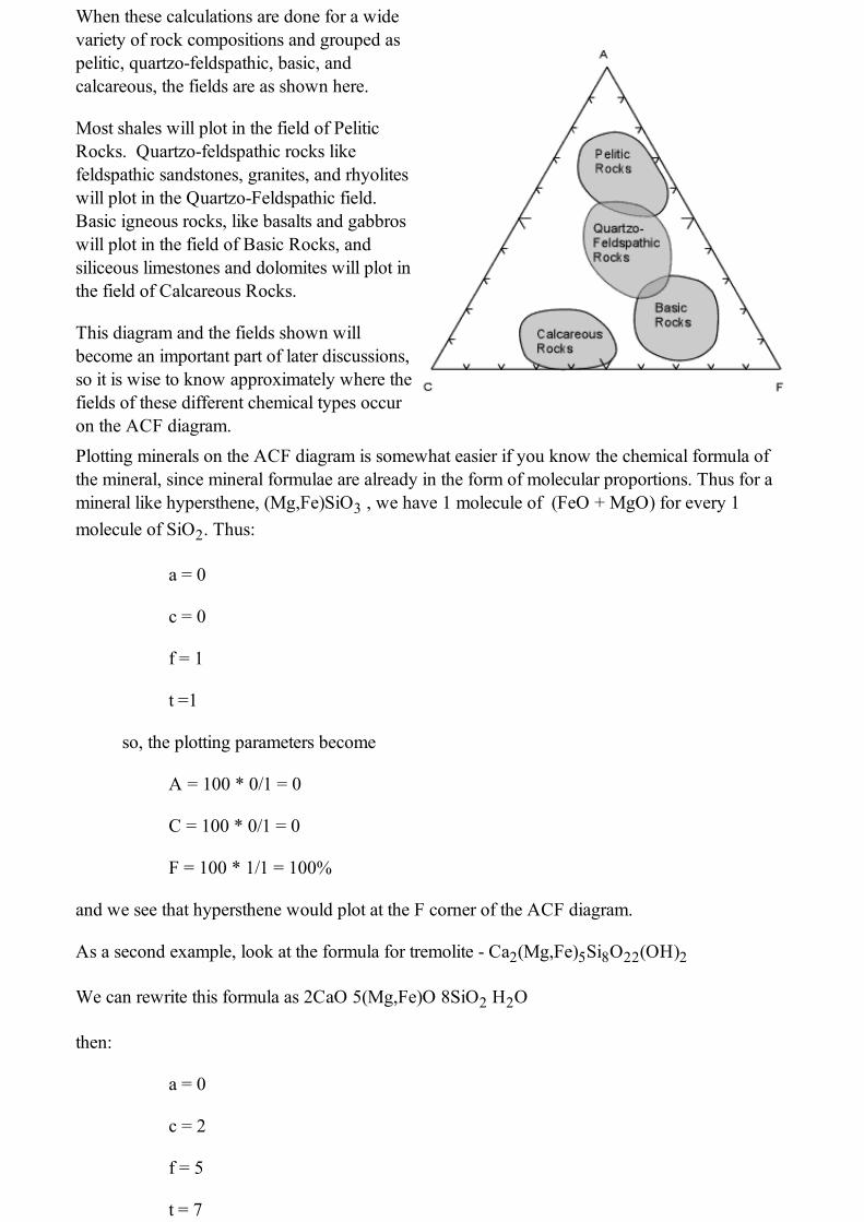
When these calculations are done for a widevariety of rock compositions and grouped aspelitic, quartzo­feldspathic, basic, andcalcareous, the fields are as shown here.

Most shales will plot in the field of PeliticRocks.  Quartzo­feldspathic rocks likefeldspathic sandstones, granites, and rhyoliteswill plot in the Quartzo­Feldspathic field. Basic igneous rocks, like basalts and gabbroswill plot in the field of Basic Rocks, andsiliceous limestones and dolomites will plot inthe field of Calcareous Rocks.  

This diagram and the fields shown willbecome an important part of later discussions,so it is wise to know approximately where thefields of these different chemical types occuron the ACF diagram. Plotting minerals on the ACF diagram is somewhat easier if you know the chemical formula ofthe mineral, since mineral formulae are already in the form of molecular proportions. Thus for amineral like hypersthene, (Mg,Fe)SiO3 , we have 1 molecule of  (FeO + MgO) for every 1molecule of SiO2. Thus:

a = 0

c = 0

f = 1

t =1

so, the plotting parameters become

A = 100 * 0/1 = 0

C = 100 * 0/1 = 0

F = 100 * 1/1 = 100%

and we see that hypersthene would plot at the F corner of the ACF diagram. 

As a second example, look at the formula for tremolite ­ Ca2(Mg,Fe)5Si8O22(OH)2 

We can rewrite this formula as 2CaO 5(Mg,Fe)O 8SiO2 H2O

then:

a = 0

c = 2

f = 5

t = 7

so the plotting parameters become:

A = 100 * 0/7 = 0

C = 100 * 2/7 = 28.57%

F = 100 * 5/7 = 71.43%

Other minerals are more complicated. For example, the formula for chlorite is(Mg,Al,Fe)12(Si,Al)8O20(OH)16. Thus we have several possibilities for writing the formula forchlorite, and depending on which formula we use, chlorite will plot at different locations on thediagrams. You will explore the possible solid solution ranges in  a lab on this topic.

Although you will calculate the plotting positions of some rocks and a wide variety of minerals inlab, the diagram above shows the plotting positions of some of the more common minerals thatoccur in metamorphic rocks.  Note that this diagram is for reference only, it does not showmineral assemblages in rocks (there are no tie lines).  Note that alkali feldspars do not plot in thisdiagram, but are assumed to be present because of the way we calculate the A component.

AKF Diagrams

In AKF diagrams we assume that both alkali feldspar and plagioclase feldspar can be present,thus the amount of Al2O3 that we use is the excess Al2O3 left after allotting it to all of thefeldspars. To obtain the plotting parameters for ACF diagrams, calculate the following:

a = [Al2O3 + Fe2O3] ­ [Na2O + K2O + CaO]

k = [K2O]

f = [FeO + MgO + MnO]

Let t = a + k + f, then the plotting parameters in % are:

A = 100 * a/t 

K = 100 * k/t 

F = 100 * f/t

Minerals are plotted in the same way as was done for the ACF diagrams, and an example AKFdiagram showing the potting positions of common metamorphic minerals is shown below.

Note that K­feldspar plots in the lower right hand corner. To see why, we first take the chemicalformula of K­feldspar KAlSi3O8 and rewrite it in oxide form as 1/2K2O 1/2Al2O3 3SiO2. Then:

a = ½ ­ ½ = 0

k = ½

f = 0

t = ½

So,

A = 100 * 0/½  = 0%

K = 100 * ½ /½ = 100%

F = 100 * 0/½ = 0%

Another example is muscovite KAl3Si3O10(OH)2 or 1/2K2O 3/2Al2O3 3SiO2 H2O.  Formuscovite:

a = 3/2 ­ 1/2 = 1

k = 1/2

f = 0

t = 1½ = 1.5

So,

A = 100 * 1/1.5 = 66.7%

K = 100 * 0.5/1.5 = 33.33%

F = 100 * 0 = 0%

Note that AKF diagrams are used for CaO­poor, K2O­rich rocks, whereas ACF diagrams shouldbe used for Al2O3  and CaO ­ rich rocks.

AKFM Projection onto AFM

The ACF and AKF diagrams discussed so far, are fairly simple, but useful.  One of the problemsassociated with ACF and AKF diagrams is that Fe and Mg are assumed to substitute for oneanother and act as a single component.  We know, however, that in natural minerals thecomposition of Fe ­ Mg solid solutions is very much dependent on temperature and pressure. Thus, in treating Fe and Mg as a single component, we lose some information.  Realizing this,J.B. Thompson developed a projected diagram that takes into account possible variation in theMg/(Mg+Fe) ratios in ferromagnesium minerals, and has proven very useful in understandingmetamorphosed pelitic sediments. 

Thompson starts with the 5 component system SiO2 ­ Al2O3 ­ K2O ­ FeO ­ MgO  and ignoresminor components in pelitic rocks like CaO and Na2O.  Because quartz is a ubiquitous phase inmetamorphosed pelitic rocks, the five component system is projected into the four componentsystem Al2O3 ­ K2O ­ FeO ­ MgO as shown below. Next, because muscovite is also a common mineral in these rocks, all compositions are projectedfrom muscovite onto the front face of the diagram. (Al2O3 ­ FeO ­ MgO). The front face of thediagram becomes the AFM diagram.

Minerals that contain no K2O like andalusite, kyanite and sillimanite plot at the A corner of thediagram, and minerals like staurolite, chloritoid (Ctd), chlorite, and garnet plot on the front face ofthe diagram.

Biotite, however, does contain K2Oand has varying amounts of Al2O3 and thus is a solid solutionthat lies in the four component system. Because muscovite is relatively K ­ poor, this results inbiotite being projected to negative values of Al2O3.

Any rock composition, like composition a, shown in the diagram, will also project to the frontface, and may or may not plot at negative values of Al2O3. 

To calculate the plotting parameters for the AFM diagram the following formulae are used:

A = [Al2O3 ­ 3 K2O]

F = [FeO]

M = [MgO]

Using these parameters, one can grid off the AFM diagram with the vertical scale represented bythe normalized values for the A parameter ­

[Al2O3 ­ 3 K2O]/[Al2O3 ­ 3 K2O + FeO + MgO]

and the horizontal position based on the ratio of MgO/(FeO + Mg). as seem below.  Of coursethese values are obtained after converting the chemical analysis of the rock to molecularproportions.

Note that if we project K­spar from muscovite, that the arrow points toward the K corner of the 4component tetrahedron, and thus K­spar would project away from the front face of the diagram. Thus, as seen on the AFM face, K­spar would plot at negative infinity.The projection from muscovite works well for metamorphic rocks that contain muscovite.  But, athigher grades of metamorphism, in the upper amphibolite facies and the granulite facies,muscovite becomes unstable and is replaced by K­feldspar + quartz + an Al2SiO5 mineral.  Inorder to show rocks and mineral assemblages at these higher grades of metamorphism, a newprojection is made from K­spar, as shown below.For this diagram the plottingparameters are much more straightforward, with ­

A = [Al2O3]

F= [FeO]

M =[ MgO]

All on a molecular basis and thenrenormalized to sum to 100%.

Note the absence of all hydrousphases (staurolite, chloritoid,muscovite) except biotite in thisprojection. 

Resolving Problems

As soon as we start ignoring components or projecting into three component compositiondiagrams there is a potential to lose information.  Sometimes the loss of information creates a

dilemma that must be resolved in order to understand the mineral assemblage.

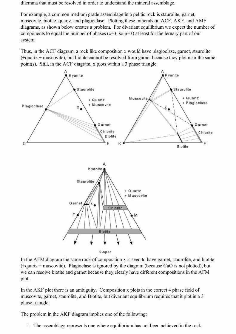
For example, a common medium grade assemblage in a pelitic rock is staurolite, garnet,muscovite, biotite, quartz, and plagioclase.  Plotting these minerals on ACF, AKF, and AMFdiagrams, as shown below creates a problem.  For divariant equilibrium we expect the number ofcomponents to equal the number of phases (c=3, so p=3) at least for the ternary part of oursystem. 

Thus, in the ACF diagram, a rock like composition x would have plagioclase, garnet, staurolite(+quartz + muscovite), but biotite cannot be resolved from garnet because they plot near the samepoint(s).  Still, in the ACF diagram, x plots within a 3 phase triangle. 

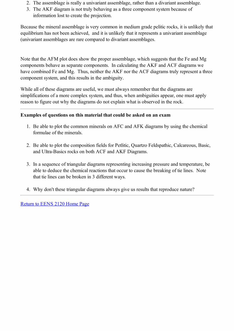
In the AFM diagram the same rock of composition x is seen to have garnet, staurolite, and biotite(+quartz + muscovite).  Plagioclase is ignored by the diagram (because CaO is not plotted), butwe can resolve biotite and garnet because they clearly have different compositions in the AFMplot.

In the AKF plot there is an ambiguity.  Composition x plots in the correct 4 phase field ofmuscovite, garnet, staurolite, and Biotite, but divariant equilibrium requires that it plot in a 3phase triangle.  

The problem in the AKF diagram implies one of the following:

1.  The assemblage represents one where equilibrium has not been achieved in the rock.

2.  The assemblage is really a univariant assemblage, rather than a divariant assemblage.3.  The AKF diagram is not truly behaving as a three component system because of

information lost to create the projection.

Because the mineral assemblage is very common in medium grade pelitic rocks, it is unlikely thatequilibrium has not been achieved,  and it is unlikely that it represents a univariant assemblage(univariant assemblages are rare compared to divariant assemblages. 

Note that the AFM plot does show the proper assemblage, which suggests that the Fe and Mgcomponents behave as separate components.  In calculating the AKF and ACF diagrams wehave combined Fe and Mg.  Thus, neither the AKF nor the ACF diagrams truly represent a threecomponent system, and this results in the ambiguity.

While all of these diagrams are useful, we must always remember that the diagrams aresimplifications of a more complex system, and thus, when ambiguities appear, one must applyreason to figure out why the diagrams do not explain what is observed in the rock.

Examples of questions on this material that could be asked on an exam

1.  Be able to plot the common minerals on AFC and AFK diagrams by using the chemicalformulae of the minerals.  

2.  Be able to plot the composition fields for Petlitic, Quartzo Feldspathic, Calcareous, Basic,and Ultra­Basics rocks on both ACF and AKF Diagrams.

3.  In a sequence of triangular diagrams representing increasing pressure and temperature, beable to deduce the chemical reactions that occur to cause the breaking of tie lines.  Notethat tie lines can be broken in 3 different ways.

4.  Why don't these triangular diagrams always give us results that reproduce nature?

Return to EENS 2120 Home Page