Triangle geometry for qutrit states in the probability representation.

V. N. Chernega1, O. V. Man’ko1,2, V. I. Man’ko1,3,4

1 - Lebedev Physical Institute, Russian Academy of Sciences

Leninskii Prospect 53, Moscow 119991, Russia

2 - Bauman Moscow State Technical University

The 2nd Baumanskaya Str. 5, Moscow 105005, Russia

3 - Moscow Institute of Physics and Technology (State University)

Institutskii per. 9, Dolgoprudnyi, Moscow Region 141700, Russia

4 Tomsk State University, Department of Physics

Lenin Avenue 36, Tomsk 634050, Russia

Corresponding author e-mail: manko@sci.lebedev.ru

Abstract

We express the matrix elements of the density matrix of the qutrit state in terms of

probabilities associated with artificial qubit states. We show that the quantum statistics

of qubit states and observables is formally equivalent to the statistics of classical systems

with three random vector variables and three classical probability distributions obeying

special constrains found in this study. The Bloch spheres geometry of qubit states is

mapped onto triangle geometry of qubits. We investigate the triada of Malevich’s squares

describing the qubit states in quantum suprematism picture and the inequalities for the

areas of the squares for qutrit (spin-1 system). We expressed quantum channels for qutrit

states in terms of a linear transform of the probabilities determining the qutrit-state

density matrix.

1 Introduction

The pure states of qutrit are described by a vector in the three-dimensional Hilbert

space [1]. The mixed states of qutrit are described by the three-dimensional density

1

arX

iv:1

804.

0488

6v1

[qu

ant-

ph]

13

Apr

201

8

matrix [2]. The qutrit states can be realized as the states of a spin-1 particle or as the

states of the three-level atom. The density matrix of the spin state in the spin tomo-

graphic probability representation [3, 4] is determined by a fair probability distribution of

spin projections on arbitrary directions in the space called the spin tomogram. The von

Neumann entropy [5] of the qutrit state was shown [6] to satisfy the entropic inequality,

which is the subadditivity condition analogous to the subadditivity condition for bipartite

systems of two qubits. Recently [7, 8], the triangle geometry of qubit states, in which

the density matrix of the spin-1/2 particle was associated with the triada of Malevich’s

squares, was investigated. The areas of the Malevich’s squares are determined by three

tomographic probabilities of spin projections m = 1/2 onto three perpendicular directions

in the space.

The aim of this work is to construct the triada of Malevich’s squares associated with

the density matrix of qutrit states using the approach connecting the qutrit states with

the states of two artificial qubits found in [6] and extra artificial qubit associated with

the permutation of the axes x ←→ z in the three-dimensional space. We review the

probability description of qubit states [7, 8, 9] and derive compact formulas for spin

tomograms of these states. We use the relation of quitrit states to the states of artificial

qubits to express the density matrix elements of the qutrit state in terms of probabilities

of the spin-1/2 projection.

This paper is organized as follows.

In Sec. 2, we review the quantum suprematism picture of spin-1/2 particle states

suggested in [7, 8]. In Sec. 3, we discuss the statistical properties of the quantum spin-1/2

observable. In Sec. 4, we consider the qutrit-state density matrix and express its matrix

elements in terms of probabilities of spin-1/2 projections related to three artificial qubit

states connected with the given indivisible qutrit system. In Sec. 5, we discuss the triangle

geometry of the qutrit state and study the inequalities for the tomographic probabilities

determining the state density matrix. We present our conclusions and prospectives in

Sec. 6.

2

2 Qubits in the Quantum Suprematism Picture

The density matrix of qubit states is the Hermitian 2×2 matrix ρ satisfying the conditions

ρ† = ρ, Trρ = 1, and ρ ≥ 0. This means that the density matrix has two eigenvalues,

which are nonnegative numbers λ1 and λ2, with λ1 + λ2 = 1. We consider the matrix

ρ =

ρ11 ρ12

ρ21 ρ22

. The eigenvalues λ1 and λ2 of the density matrix ρ satisfy the equation

(ρ11 − λ) (ρ22 − λ)− ρ12ρ21 = 0. (1)

It was shown in [9] that the matrix elements of the density matrix ρ can be expressed

within the framework of the probability representation of qubit states in terms of three

probabilities 0 ≤ p1, p2, p3 ≤ 1, namely,

ρ =

p3 p1 − ip2 − (1/2) + (i/2)

p1 + ip2 − (1/2)− (i/2) 1− p3

. (2)

In this expression, nonnegative probabilities p1, p2, and p3 are the probabilities of spin-

1/2 projections m = 1/2 onto three perpendicular directions in the space, namely, p1 is

the probability to have the spin projection along the x direction, p2 is the probability to

have the spin projection along the y direction, and p3 is the probability to have the spin

projection along the z direction. The eigenvalues of the density matrix (2) read

λ1 =1

2+

3∑j=1

(pj −

1

2

)21/2 , λ2 =

1

2−

3∑j=1

(pj −

1

2

)21/2 . (3)

The nonnegativity of the density matrix provides the inequality [9] for three probabilities

pj, namely,

(p1 − 1/2)2 + (p2 − 1/2)2 + (p3 − 1/2)2 ≤ 1/4. (4)

This inequality is the nonnegativity condition for the density matrix of the qubit state; it

reflects the presence of quantum correlations of the single-spin states.

There exists the geometrical interpretation of the introduced parameters of the spin-

state density matrix. The probabilities p1, p2, and p3 can be associated with a triangle on

the plane [7, 8]. The lengths Ln (n = 1, 2, 3) of the triangle sides are expressed in terms

of the probabilities as follows:

L1 =(2 + 2p22 − 4p2 − 2p3 + 2p23 + 2p2p3

)1/2,

3

L2 =(2 + 2p23 − 4p3 − 2p1 + 2p21 + 2p3p1

)1/2, (5)

L3 =(2 + 2p21 − 4p1 − 2p2 + 2p22 + 2p1p2

)1/2.

The probabilities p1, p2, and p3 satisfy the inequality

Ln + Ln−1 > Ln+1, n = 1, 2, 3. (6)

Three squares with these sides and the areas Sn = L2n were introduced in [7, 8]; they were

called the triada of Malevich’s squares. The area of triangle with the sides Ln reads

Str = (1/4)[ (L1 + L2 + L3) (L1 + L2 − L3) (L2 + L3 − L1) (L3 + L1 − L2) ]1/2. (7)

Usually, the density matrix (2) is associated with a point in the Bloch ball. In the triangle

geometry picture under discussion, the density matrix is represented by the triada of

Malevich’s squares. This means that we construct the invertible map of any point in

the Bloch ball onto the triangle with sides Ln and the triada of Malevich’s squares. The

obvious inequalities for the triangle sides give the inequalities for the probabilities p1, p2,

and p3 (6). These inequalities are compatible with the condition (4). The three squares

introduced in [7, 8] and called the triada of Malevich’s squares provide the quantum

suprematism picture of the qubit states.1 It is worth noting that Zeilinger, emphasizing

in [10] the importance in physics to make experiments as simple as possible and with the

smallest efforts, compared such approach with the creation of Malevich’s black square in

the art.

The sum of areas of three Malevich’s squares expressed in terms of the probabilities

p1, p2, and p3 reads

S = 2[3 (1− p1 − p2 − p3) + 2p21 + 2p22 + 2p23 + p1p2 + p2p3 + p3p1

]. (8)

The sum satisfies the inequality

3/2 ≤ S < 9/2. (9)

For classical system of three coins, an analogous suprematism picture of Malevich’s squares

provides for this sum the domain 3/2 ≤ S ≤ 6. The difference between numbers 9/2 and

6 reflects the difference of classical and quantum correlations in the two systems – qubit

1We thank Dr. Tommaso Calarco for informing us about available discussions of Malevich’s square

picture related to quantum states of a single atom (private communication).

4

and three coins, though the states in both cases are determined by three probabilities p1,

p2, and p3.

3 Statistical Properties of Quantum Observable

In this section, we discuss the properties of means of an observable A given by the Her-

mitian matrix Ajk =

A11 A12

A21 A22

. The mean values of the observable in the state with

the density matrix (2) read

〈A〉 = TrAρ = p3A11+(1−p3)A22+A12(p1+ip2−(1+i)/2)+A21(p1−ip2−(1− i)/2). (10)

This relation can be interpreted using the picture of three classical random observables,

which are described by three probability distributions.

In fact, there are three probability vectors

~P1 =

p1

1− p1

, ~P2 =

p2

1− p2

, ~P3 =

p3

1− p3

.For a spin-1/2 system, probabilities (1−p1), (1−p2), and (1−p3) are the probabilities to

have the spin-projection m = −1/2 along the axes x, y, and z, respectively. The matrix

elements of the matrix Ajk (j, k = 1, 2) can be considered as linear functions of classical

random variables, which take the real values

X1 =A12 + A21

2, Y1 =

i(A12 − A21)

2, X2 = −A12 + A21

2, Y2 = −i(A12 − A21)

2(11)

and

Z1 = A11, Z2 = A22. (12)

The inverse relations are

A12 = X1 − iY1, A11 = Z1, A22 = Z2, A21 = X1 + iY1. (13)

Introducing the vector notation for the classical variables

~X =

X1

X2

, ~Y =

Y1

Y2

, ~Z =

Z1

Z2

, (14)

5

we obtain the expression for the mean value of quantum observable 〈A〉 in terms of the

mean values of classical observables ~X, ~Y , and ~Z of the form

〈A〉 = ~P1~X + ~P2

~Y + ~P3~Z. (15)

Thus, the quantum relation for the mean value of the spin observable A in the state with

the density matrix ρ given by (2) is presented as the sum of three classical means of

random variables ~X, ~Y , and ~Z,

〈A〉 = p1X1 + (1− p1)X2 + p2Y1 + (1− p2)Y2 + p3Z1 + (1− p3)Z2. (16)

These observations provide a possibility to construct the model of quantum observable A

using the classical observables ~X, ~Y , and ~Z.

In fact, for given arbitrary three real two-vectors ~X, ~Y , and ~Z such that X1 + X2 =

Y1 + Y2 = 0, we construct the Hermitian matrix Ajk (j, k = 1, 2) with matrix elements

(13). Since the density matrix (2) is expressed in terms of classical probability vectors

~P1, ~P2, and ~P3, the measurable quantum observable A has the mean value determined by

classical observables ~X, ~Y , ~Z and classical probability distributions.

Quantumness of the model is formulated as inequality (4) reflecting the condition for

classical probabilities p1, p2, and p3, and the definition of the second moment of quantum

observable 〈A2〉 in terms of classical random variables ~X, ~Y , and ~Z,

TrρA2 = p3Z21 − (1− p3)Z2

2 +X21 + Y 2

1 + 2(Z1 + Z2)[X1(p1 − 1/2) + Y1(p2 − 1/2)]

= (Z1 + Z2)[~X ~P1 + ~Y ~P2

]+ (X2

1 + Y 21 ) + p3(Z

21 − Z2

2) + Z22 . (17)

The constructed relations (13)–(16) and formulas (16) and (17) for the quantum mean

and dispersion of any observable A, expressed in term of classical random variables and

classical probabilities, demonstrate that quantum mechanics of qubits can be formulated

using only standard ingredients of classical probability theory. We conjecture that quan-

tum mechanics of any qudit system can also be formulated using only classical random

variables and classical probability distributions. The difference from classical statisti-

cal mechanics is expressed by specific inequalities for classical probability distributions,

reflecting hidden correlations in quantum systems analogous to (4) for qubits.

6

4 Qutrit in the Probability Representation

The tomographic probability distribution for the spin-1 system for a minimum number of

probabilities can be described by eight parameters, which are spin projections m = +1, 0

onto four directions; these probabilities are discussed in [9]. In this section, we develop

another approach to associate the density matrix of the qutrit state with probabilities

determining the states of artificial qubits.

We follow the approach applied to get a new entropic subadditivity condition for the

qutrit state suggested in [6]. The density matrix of the spin-1 system is given by the

matrix ρ, such that ρ† = ρ, Trρ = 1, and ρ ≥ 0; it reads

ρ =

ρ11 ρ12 ρ13

ρ21 ρ22 ρ23

ρ31 ρ32 ρ33

. (18)

Applying the tool to consider the matrix ρ as the 3×3 block matrix in the 4×4 density

matrix of two qubits with zero fourth column and zero fourth row, we obtain two qubit-

state density matrices of the artificial qubits using the partial tracing procedure. The

2×2 matrices are

ρ(1) =

ρ11 + ρ22 ρ13

ρ31 ρ33

, ρ(2) =

ρ11 + ρ33 ρ12

ρ21 ρ22

. (19)

For these two qubit-state density matrices, we have the expressions in the probability

representation in terms of probabilities p(k)1,2,3, k = 1, 2, of the form

ρ(k) =

p(k)3 p

(k)1 − ip

(k)2 − (1/2) + (i/2)

p(k)1 + ip

(k)2 − (1/2)− (i/2) 1− p(k)3

, k = 1, 2. (20)

This means that a part of the matrix elements of the density matrix ρ is expressed in

terms of the probabilities p(k)j , k = 1, 2, j = 1, 2, 3, namely,

ρ11 = p(2)3 − (1− p(1)3 ), ρ22 = 1− p(2)3 , ρ33 = 1− p(1)3 . (21)

For off-diagonal matrix elements, we have

ρ12 = p(2)1 − ip

(2)2 − (1/2) + (i/2), ρ21 = ρ∗12, (22)

ρ13 = p(1)1 − ip

(1)2 − (1/2) + (i/2), ρ31 = ρ∗13. (23)

7

To obtain an explicit expression for the matrix element ρ23 in terms of probabilities, we

consider the density matrix of the state where we use the permutation of axes x↔ z; this

means that we use another qutrit state. For a three-level atom, we use the permutation

of the ground state level and maximum excited energy level; in such a case, we have the

extra qubit with the density matrix

ρ(3) =

ρ33 + ρ11 ρ32

ρ23 ρ22

. (24)

The probabilities p(3)j for this artificial qubit state read

p(3)3 = ρ11 + ρ33 = p

(2)3 , p

(3)1 − ip

(3)2 − (1− i)/2 = ρ32, ρ23 = ρ∗32. (25)

Thus, we provide the final expression of the qutrit density matrix ρ in terms of eight

parameters – probabilities p(1)1 , p

(1)2 , p

(1)3 , p

(2)1 , p

(2)2 , p

(2)3 , p

(3)1 , and p

(3)2 . The density matrix

ρ is

ρ =

p(2)3 + p

(1)3 − 1 p

(2)1 − ip

(2)2 − (1− i)/2 p

(1)1 + ip

(1)2 − (1 + i)/2

p(2)1 + ip

(2)2 − (1 + i)/2 1− p(2)3 p

(3)1 + ip

(3)2 − (1 + i)/2

p(1)1 − ip

(1)2 − (1− i)/2 p

(3)1 − ip

(3)2 − (1− i)/2 1− p(1)3

. (26)

The parameters p(k)j , k, j = 1, 2, 3 must satisfy the inequalities

3∑j=1

(p(k)j − 1/2)2 ≤ 1/4. (27)

In addition to these inequalities, one has the cubic inequality det ρ ≥ 0 and the quadratic

inequality like

(1− p(2)3 ) (1− p(1)3 )− |p(3)1 + ip(3)2 − (1 + i)/2|2 ≥ 0. (28)

To check all the inequalities, one needs to provide the probabilities of spin-projections

m = +1/2 onto three perpendicular directions for the three artificial qubits. For the

two qubits, the directions are given by the axes x, y, and z, and for the third qubit the

direction corresponds to the permutation of the first and the third directions, x↔ z.

The density matrix ρ can be rewritten in the form

ρ =

p(2)3 + p

(1)3 − 1 p(2)∗ − γ∗ p(1) − γ

p(2) − γ 1− p(2)3 p(3) − γ

p(1)∗ − γ∗ p(3)∗ − γ∗ 1− p(1)3

, (29)

8

where the complex numbers p(k) are p(k) = p(k)1 +ip

(k)2 , k = 1, 2, 3, and γ = (1+i)/2. Then

we express the purity of the qutrit state µ = Trρ2 in terms of three classical probabilities

p(k)j , j, k = 1, 2, 3,

µ = (p(2)3 +p

(1)3 −1)2 +(1−p(2)3 )2 +(1−p(1)3 )2 +2[|p(1)−γ|2 + |p(2)−γ|2 + |p(3)−γ|2]. (30)

The nonnegativity condition of the density matrix det ρ ≥ 0 yields the inequality for the

probabilities p(k)j , which looks like the inequality for the cubic polynomial,

(p(2)3 + p

(1)3 − 1)(1− p(2)3 )(1− p(1)3 ) + (p(2) − γ)(p(1) − γ)(p(3)∗ − γ∗)

+(p(2)∗ − γ∗)(p(1)∗ − γ∗)(p(3) − γ)− |p(1)∗ − γ∗|2(1− p(2)3 )− |p(2) − γ|2(1− p(1)3 )

−|p(3) − γ|2(p(2)3 + p(1)3 − 1) ≥ 0. (31)

The obtained inequalities (27), (28), and (31) are quantum characteristics of the qutrit

state expressed in terms of classical probabilities p(k)j . One can extend the model of qubit

state based on the properties of classical random variables ~X, ~Y , and ~Z (14) to the case

of the qutrit state. We consider random classical variables ~X(k), ~Y (k), and ~Z(k), k = 1, 2, 3

with the probability distributions given by the vectors ~P(k)1 , ~P(k)

2 , and ~P(k)3 .

If inequalities (27), (28), and (31) are not valid, the system properties correspond to

the behavior of sets of classical “coins.” Namely, quantum correlations are described by

inequalities (27), (28), and (31). Thus, we obtain new inequalities for qutrit states, which

are entropic inequalities for the probability vectors ~P(k)j , j, k = 1, 2, 3. For example, the

inequality for relative entropy

2∑j=1

p(k)j ln ( p

(k)j /p

(k′)j ) ≥ 0, k, k′ = 1, 2, 3, (32)

is valid for two arbitrary probability distributions. Since the probabilities are expressed in

terms of the density matrix elements of the qutrit state, one has new entropic inequalities

for the qutrit-state density matrix; it is just inequality (32), which provides the entropic

inequality for the matrix elements of the qutrit-state density matrix.

For example, one has the new relative-entropy inequality for the matrix elements of

the qutrit-state density matrix

1

2(ρ12 + ρ21 + 1) ln

[ρ12 + ρ21 + 1

ρ13 + ρ31 + 1

]+

1

2[i(ρ12 − ρ21)− 1] ln

[i(ρ12 − ρ21)− 1

i(ρ13 − ρ31)− 1

]≥ 0. (33)

9

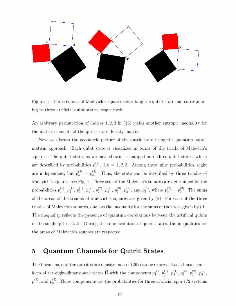
Figure 1: Three triadas of Malevich’s squares describing the qutrit state and correspond-

ing to three artificial qubit states, respectively.

An arbitrary permutation of indices 1, 2, 3 in (33) yields another entropic inequality for

the matrix elements of the qutrit-state density matrix.

Now we discuss the geometric picture of the qutrit state using the quantum supre-

matism approach. Each qubit state is visualized in terms of the triada of Malevich’s

squares. The qutrit state, as we have shown, is mapped onto three qubit states, which

are described by probabilities p(k)j , j, k = 1, 2, 3. Among these nine probabilities, eight

are independent, but p(3)3 = p

(2)3 . Thus, the state can be described by three triadas of

Malevich’s squares; see Fig. 1. Three sets of the Malevich’s squares are determined by the

probabilities p(1)1 , p

(1)2 , p

(1)3 , p

(2)1 , p

(2)2 , p

(2)3 , p

(3)1 , p

(3)2 , and p

(3)3 , where p

(2)3 = p

(3)3 . The sums

of the areas of the triadas of Malevich’s squares are given by (8). For each of the three

triadas of Malevich’s squares, one has the inequality for the sums of the areas given by (9).

The inequality reflects the presence of quantum correlations between the artificial qubits

in the single-qutrit state. During the time evolution of qutrit states, the inequalities for

the areas of Malevich’s squares are respected.

5 Quantum Channels for Qutrit States

The linear maps of the qutrit-state density matrix (26) can be expressed as a linear trans-

form of the eight-dimensional vector ~Π with the components p(1)1 , p

(1)2 , p

(1)3 , p

(2)1 , p

(2)2 , p

(2)3 ,

p(3)1 , and p

(3)2 . These components are the probabilities for three artificial spin-1/2 systems

10

and three spin projections m = 1/2 onto three perpendicular directions in the space. In

fact, we have also the probabilities p(3)3 = p

(2)3 . The unitary transform of the density

matrix ρ

ρ −→ ρu = uρu†, (34)

where uu† = 1, provides the linear transform of the eight-vector ~Π. One can get this

transform (quantum channel) in an explicit form.

In fact, the nine-dimensional vector ~ρ with components (ρ11, ρ12, ρ13, ρ21, ρ22, ρ23, ρ31, ρ32, ρ33),

which can be denoted as (ρ1, ρ2, ρ3, ρ4, ρ5, ρ6, ρ7, ρ8, ρ9), after the unitary transform con-

verts to the vector ~ρu = u⊗ u∗~ρ. Then we arrive at

Π′k =8∑

j=1

UkjΠj + Γk, (35)

where the 9×9 unitary matrix U = u⊗ u∗ determines the 8×8 matrix Ukj and the eight-

vector ~Γ.

Since the components of vectors ~Π and ~Π′ are expressed in terms of the probabil-

ities p(k)j and p

(k)′

j , the channel under discussion provides an explicit transform of the

probabilities determining the qutrit density matrices. For a unital channel of the form

ρ −→ ρU =∑

k pkukρu†k (0 ≥ pk ≥ 0,

∑k pk = 1), the transform of the vector ~ρ −→ ~ρU

reads

~ρU =

(∑k

pkuk ⊗ u∗k

)~ρ. (36)

It provides the transform of the eight-vector ~Π −→ ~ΠU of the form

~ΠU =

(∑k

pkUk

)~Π + ~Γ, (37)

where the eight-vectors ~Π and ~ΠU are expressed in terms of eight probabilities determining

the qutrit-state density matrix ρ. An analogous relation describes the generic completely

positive map of the qutrit-state density matrix

ρ −→ ρpos =∑k

VkρV†k , (38)

where Vk are arbitrary 3×3 matrices satisfying the relation∑

k V†k Vk = 1 .

For example, the channel providing the transform ρkk −→ ρ′kk = ρkk and ρkj −→

ρ′kj = 0 (k 6= j) for the qutrit-state density matrix determines the transform of the

probabilities p(k)′

1 = 1/2, p(k)′

2 = 1/2, p(k)′

3 = p(k)3 , k = 1, 2, 3. This means that

11

such a channel transforms the states of three artificial qubits determining the initial

density matrix of the qutrit state into the state with maximum entropy S = ln 2 for

the probability distributions of spin-projections m = ±1/2 along the axes x and y. The

positive map can be determined by the combination of the described maps with the

transforms ρ(1) −→ ρtr(1) and ρ(2) −→ ρtr(2) of the two artificial qubit-state density

matrices, as well as an analogous transposition of the third artificial qubit-state density

matrix.

6 Conclusions

To conclude, we point out the main results of this work.

We presented the matrix elements of the qutrit-state density matrix as linear combi-

nations of nine classical probabilities p(1)1 , p

(1)2 , p

(1)3 , p

(2)1 , p

(2)2 , p

(2)3 , p

(3)1 , p

(3)2 = p

(3)3 . We

interpreted the probabilities p(k)j , j, k = 1, 2, 3 as the probabilities to have “spin-1/2 pro-

jections” m = 1/2 in three perpendicular directions of three artificial qubits. This means

that such quantum system as qutrit has states whose density matrices are given in the

classical formulation by eight independent parameters – eight probabilities corresponding

to the states of eight classical coins.

We found new inequalities for the introduced classical probabilities, including new

entropic inequalities for the qutrit-state density matrix elements. The new inequalities

provide the condition of quantumness of qutrit. The states of eight classical coins are

described by the same probabilities, but these probabilities should not satisfy these con-

strains. The new relations for the qutrit-state density matrices obtained can be checked

in experiments with superconducting circuits [11] based on Josephson junctions, which

have been discussed in connection with the nonstationary (dynamical) Casimir effect

in [12, 13, 14, 15]; see also recent publications [16, 17, 18, 19, 20, 21, 22]. The dynamical

Casimir effect was discovered in [23] and discussed in [24, 25, 26, 27].

We presented the observables of the spin-1/2 system in the form of three classical

random variables ~X, ~Y , and ~Z, which are described by classical probability vectors ~P1,

~P2, and ~P3. These three classical variables are organized in the form of the Hermitian

matrix. The quantumness of the construction is reflected by the introduced inequalities

12

for the probability distributions. We extended an analogous construction for qutrit states

and observables. We discussed quantum channels for qutrit states in the probability

representation. Some aspects of the quantum channel properties in the tomographic-

probability picture are presented in [28, 29]. We considered the triangle geometry of qutrit

states and described the states by the three triadas of Malevich’s squares in the quantum

suprematism approach (suprematism in the art is reviewed in [30]). The consideration

can be extended to arbitrary systems of qudit states. We will study this problem in a

future publication.

Acknowledgments

The formulation of the problem of quantum suprematism and the results of Sec. 2 are

due to V. I. Man’ko, who is supported by the Russian Science Foundation under Project

No. 16-11-00084; the work was partially performed at the Moscow Institute of Physics

and Technology.

References

[1] P. Dirac, The Principles of Quantum Mechanics, Oxford University Press (1930).

[2] L. D. Landau, Z. Phys., 45, 430 (1927).

[3] V. V. Dodonov and V. I. Man’ko, Phys. Lett. A, 239, 335 (1997).

[4] V. I. Man’ko and O. V. Man’ko, J. Exp. Theor. Phys., 85, 430 (1997).

[5] J. von Neumann, Mathematische Grundlagen der Quantenmechanik, Springer, Berlin

(1932).

[6] V. N. Chernega, O. V. Manko, and V. I. Manko, J. Russ. Laser Res., 34, 383 (2013).

[7] V. N. Chernega, O. V. Man’ko, and V. I. Man’ko, J. Russ. Laser Res., 38, 141 (2017).

[8] V. N. Chernega, O. V. Man’ko, and V. I. Man’ko, J. Russ. Laser Res., 38, 324 (2017).

[9] V. I. Man’ko, G. Marmo, F. Ventriglia, and P. Vitale, J. Phys. A: Math. Gen., 50,

335302 (2017); arXiv:1612.07986 (2016).

13

[10] A. Zeilinger, Phys. Scr., 92, 072501 (2017).

[11] T. Fujii, Sh. Matsuo, N. Hatakenaka, et al., Phys. Rev. B, 84, 174521 (2011).

[12] V. V. Dodonov, V. I. Man’ko, and O. V. Man’ko, J. Sov. Laser Res., 10, 413 (1989).

[13] V. I. Man’ko, J. Sov. Laser Res., 12, 383 (1991).

[14] O. V. Man’ko, J. Korean Phys. Soc., 27, 1 (1994).

[15] V. V. Dodonov, V. I. Man’ko, and O. V. Man’ko, Meas. Tech., 33, 102 (1990).

[16] A. K. Fedorov, E. O. Kiktenko, O. V. Man’ko, and V. I. Man’ko, Phys. Scr.. 90,

055101 (2015).

[17] O. V. Man’ko, AIP Conf. Proc., 1424, 221 (2012).

[18] O. V. Man’ko, Phys. Scr., T153, 014046 (2013).

[19] A. K. Fedorov, E. O. Kiktenko, O. V. Man’ko, and V. I. Man’ko, Phys. Rev. A, 91,

042312 (2015).

[20] M. H. Devoret and R. J. Schoelkopf, Science, 339, 1169 (2013).

[21] Y. A. Pashkin, T. Yamamoto, O. Astafiev, et al., Nature, 421, 823 (2003).

[22] A. Averkin, A. Karpov, K. Shulga, et al., Rev. Sci. Instrum., 85, 104702 (2014).

[23] C. N. Wilson, G. Johansson, A. Pourkabirian, et al., Nature, 479, 376 (2011).

[24] V. V. Dodonov, Adv. Chem. Phys., 119, 309 (2001).

[25] A. V. Dodonov, E. V. Dodonov, and V. V. Dodonov, Phys. Lett. A, 317, 378 (2003).

[26] V. V. Dodonov and A. V. Dodonov, J. Russ. Laser Res., 26, 445 (2005).

[27] V. V. Dodonov, Phys. Scr., 82, 038105 (2010).

[28] M. A. Man’ko, V. I. Man’ko, and R. V. Mendes, J. Russ. Laser Res., 27, 506 (2006).

[29] G. G. Amosov, S. Mancini, and V. I. Man’ko, “Tomographic portrait of quantum

channels,” arXiv quant-ph 1708.07697; Rep. Mat. Phys. (2017, in press).

14

[30] A. Shatskikh, Black Square: Malevich and the Origin of Suprematism, Yale Univer-

sity Press, New Haven (2012).

15