JOURNAL OF GEOPHYSICAL RESEARCH, VOL. 106, NO. D24, PAGES 33,909-33,918, DECEMBER 27, 2001

Trend surface analysis of Greenland accumulation C. J. van der Veen, • D. H. Bromwich, • B. M. Csatho, and C. Kim • Byrd Polar Research Center, Ohio State University, Columbus, Ohio

Abstract. Multivariate regression methods are applied to •neasurements of accumulation covering much of the interior of the Greenland ice sheet to evaluate the important factors that describe the current distribution of accumulation. Predictor variables considered in the

regressions are geographical coordinates and three independent factors describing the geometry of the ice sheet. The results indicate that most of the variance in the data is explained by the combined effect of large-scale atmospheric circulation and ice sheet topographyø This finding implies that climate change scenarios in which changes in accumulation are mostly associated with changes in temperature or some other parameter may only be correct if the pattern of atmospheric circulation remains unaltered. Comparison with values predicted with a precipitation retrieval model is favorable, suggesting that the model captures the most important features of Greenland precipitation.

1. Introduction

Approximately 80% of the total area of Greenland is ice cov- ered. The main ice sheet reaches thicknesses in excess of 3 km

and contains enough water to raise global sea level by 7 m if all ice were to melt. The ice cover is nourished and maintained by snowfall at higher elevations, while mass is lost through surface ablation and subsequent meltwater runoff in the coastal regions, melting underneath floating tidal glaciers, and calving at glacier tmxnini. Redistribution of mass from the accumulation area to

the marginal ablation zones is achieved through ice flow. The magnitude of each of these processes determines whether the ice sheet is in balance or whether it is growing or slu-inking• In as- sessing the state of balance of the Greenland ice sheet, it is thus important to dete•xnine accurately each term in the mass budget. In this study, the source term of average accumulation in the inte- rior is considered. The interior is defined as the region where surface elevations are in excess of 1100 m above sea level. At

these elevations the contributions to net accmnulation of mass as-

sociated with evaporation, condensation, surface ablation and runoff, and, perhaps, snowdrift are small [Oh•nura et al., 1999]. Using observations from automated weather stations, Box and Steffen [this issue] estimate sublimation over the Greenland ice sheet. Their results indicate that annual sublimation loss occurs

mostly in the ablation zone at lower elevations (<1300 m) and that near-zero loss or small net annual deposition is characteristic for the interior dry snow accumulation zone• Thus for the present study, annual precipitation rates may be equated with annual net accumulation rates. Annual accumulation is obtained from

thicknesses of annual layers observed in ice cores or shallow ice pits, corcected for density variations.

The usual procedure for computing the net accumulation or surface mass balance of the entire ice sheet is to collect point

•Also at Department of Geography, Ohio State University, Columbus, Ohio.

Copyright 2001 by the American Geophysical Union.

Paper number 2001JD900156. 0148-0227/01/2001JD900156509.00

measurements of accumulation covering most of the glacier area and interpolating these values to obtain estimates at regular grid nodes. The interpolation may consist of manually drawing con- tour lines [Ohmura and Reeh, 1991] or may involve a more ob- jective technique such as kriging [Ohmura et al., 1999; Hock and Jensen, 1999; Bales et al., this issue]. Whichever interpolation method is used, the result is a contour map showing the distribu- tion of surface accmnulation. While such a map is a valuable and necessary product for mass balance assessments and numerical modeling of ice sheet evolution, it does not convey quantitative information on factors determining the spatial distribution of ac- cumulation.

The present-day large-scale pattern of accumulation can be obtained by utilizing multiple regression techniques to derive re- lations between measured accumulation values and predictor variables. The assumption is made that accumulation is the sum of a "background" trend associated prhnarily with the large-scale atmospheric circulation, a "geometry effect" associated with the presence of the ice sheet, plus a residual term that incorporates other effects such as s•nall-scale synoptic phenomena. The first two contributions are esthnated using geographical coordinates (latitude and longitude) and factors describing the geometry of the ice sheet, as predictor variables in multivariate regression. The spatial distribution of residuals is found by la'iging and con- tom'ing the irregularly spaced differences between accumulation measurements and predictions from the regression model. This procedm'e does not, of course, establish the causality of any sta- tistically significant regression, but it is a useful exploratory tool for gaining understanding of the pattern of accumulation on the Greenland ice sheet.

The approach adopted here follows that of Mock [1967], who found that mean annual accumulation on the Greenland ice sheet

can be predicted "with a fair degree of accuracy" from the pa- rameters latitude, longitude, and elevation. The present study may be considered an update of that work in that about twice as many accumulation measurements are used, as well as a more ac- curate elevation model. Our analysis differs from most of the prior studies in which relations between accumulation and vari- ables such as annual mean temperature, surface elevation and slope, and distance to open ocean are derived [Muszynski and Birchfield, 1985; Fortuin and Oerlemans, 1990; Giovinetto et al., 1990; Giovinetto and Zwally, 1995]. The difficulty with these

33,909

33,910 VAN DER VEEN ET AL.: TREND SURFACE OF GREENLAND ACCUMULATION

regression analyses is that the rationale for selecting certain pa- rmeters only as predictor variables is not always obvious. Moreover, given the complexity of atmospheric processes, it is unlikely that regression results involving one or two predictor variables fully describe the physical processes to the extent that these linkages can be used to estimate the change in accumulation following a change in climate. To better understand the spatial distribution of accumulation and identify possible factors deter- mining this pattern, standard statistical tools for exploring spatial data [Cressie, 1993; Davis, 1986] are applied here.

Another approach to obtain the present-day large-scale pattern of accumulation is to apply precipitation modeling based on at- mospheric data, which explicitly takes into account the important dependencies [Chen et al., 1997; Chen and Bromwich, 1999; Bromwich et al., this issue]. Here we compare results from the regression analysis of measured accumulation rates with those obtained from modeling to evaluate the mutual consistency of both.

2. Statistical Model

In multivariate regression the dependent variable is assumed to be the sum of a linear combination of predictor variables plus a random error tenn. That is, the value of the dependent variable at location s, Y(s), is written as

r(s) = X(s). I• + •,

in which X(s) represents a row vector with components being the values of the predictor variables evaluated at location s and [• is the column vector of regression coefficients. The residuals or er- rors, •, are assumed to be normally distributed with constant vari- ance and to be uncorrelated. Under these conditions, estimates of

the regression coefficients can be found by minimizing the sum of the squares of the difference between predicted values and ob- servations [Draper and Smith, 1998, chapter 1]. Denoting the column vector of estimated regression coefficients as b, the val- ues predicted by the regression models are given by

•(s) = X(s). b.

A concern with applying multivariate regression to Greenland accumulation data is that the residuals of the regression model may show spatial correlation. That is, regression on geographical coordinates and ice sheet geometry may explain part of the ac- cumulation distribution, but the residuals may not be random but associated with phenomena not included in the regression model, such as storm tracks. While the general paths of storms are set up by the large-scale atmospheric circulation, there is a strong sea- sonal cycle over different parts of the ice sheet so that storms af- fect various regions differently. This means that contributions to accumulation from storms are correlated on regional scales only, and thus this contribution is not included in the large-scale trend. In that case the regression model should be modified to allow for spatial correlation of residuals. The common procedure is to make the assumption that accumulation is the combined effect of a large-scale trend on which spatially correlated patterns are su- perimposed.

To formalize the model adopted here, the dependent variable is now written as

r(s) = X(s).l• + U(s) + •.

The first term on the right-hand side represents the large-scale trend surface and can be estimated using least squares multivari-

ate regression. The second term, U(s), is a zero mean process that may exhibit autocorrelation and that represents local or sec- ond-order effects. This term is predicted at arbitrary points using kriging of the residuals (the difference between observed accu- mulation values and predictions from the regression model). As before, • represents residual random effects.

Without going into procedural details, the objective of kriging is to predict values of the spatially correlated residual at points for which there are no data. The kriging estimator t)(s) at loca- tion s is a weighted linear combination of data values U(si)at neighboring sample sites s i so that

O(S) = Z •i(s)U(si) ß i=1

The weights are chosen such that the mean residual or error, t)(s i) - U(si), equals zero if no uncertainties in the measure- ments are assumed and the variance of the errors is minimized.

For each location, weights are derived from the statistical proper- ties of the data. That is, the nature of spatial correlation must be prescribed through the variogram [cf. Isaaks and Srivastava, 1989, chapter 12].

To summarize the foregoing procedure, the following steps are involved in the statistical analysis. First, the trend surface is es- timated from multivariate regression and subtracted from the ob- servations to yield the spatially correlated residual. For these re- siduals the variogram can be calculated to find a functional ap- proximation to be used in the kriging procedure. Kriging itself is applied to interpolate the observations to regular grid points with the objective of producing a contour map of the residuals. Actual accumulation estimates at these grid points can be readily ob- tained by adding the trend surface to the estimated residuals.

It should be noted that removal of the trend sin'face is only re- quired if ordinary kriging is used for data interpolation. Univer- sal kriging can be applied to the actual data provided that the shape of the drift surface is prescribed (e.g., linear or quadratic). This drift surface is analogous to the trend surface but is based only on data points in the vicinity of the location for which a value is being estimated, and thus regional trends, rather than trends covering the entire area of study are used in universal kriging [cf. Cressie, 1993, sections 3.2 and 3.4]. However, the objective here is not to produce an accurate map of Greenland accumulation but rather to identify factors and processes that de- scribe the present-day distribution of accumulation. For this rea- son the trend surface and the spatially correlated residuals are considered separately in this study.

3. Data

In support of the NASA Program for Arctic Regional Climate Assessment (PARCA), a Greenland Geographic Information System Database System (GGDS) has been developed to inte- grate glaciological, geophysical, and geographical information [Kim et al., 2000]. The GGDS was constructed using Arc/Info and Arcview software (both from the Environmental Systems Re- search Institute), and Microsoft Access97 serves as a relational database management system. The accumulation data set of GGDS includes glaciological observations (ice cores and pits), gauge measurements (for coastal stations), and digital versions of some published accumulation maps [Ohmura and Reeh, 1991; Bender, 1984]. For the 252 ice cores and pits listed by Ohmura and Reeh [1991], the original references were investigated to

VAN DER VEEN ET AL.' TREND SURFACE OF GREENLAND ACCUMULATION 33,911

....... ?:807.... ...... / .....

..... .,/"' .//' ?'

/ ,r

?' /, /// ,/'•

f /

Figure 1. Map showing locations of accumulation measurements used in this study (dots), and surface elevation contours (contour interval is 1000 m; lowest contour is 1000 m).

validate the accumulation rate and to obtain other relevant infor-

mation such as temperature, time period, and statistics of accu- mulation rates, as well as accuracy of the observations. Recent ice cores and pits acquired by PARCA and European investiga- tors were also added. The attributes of the accumulation data are

described in more detail by Csatho et al. [1999]. The database is available online at http://sheger.mps.ohio-state.edu/.

The data set reviewed for this study is essentially the same as described by Bales et al. [this issue]. However, slightly different criteria for selecting accumulation data were applied. Only data that have been published in jom'nals or for which a detailed de- scription is available were retained. Further, the length of each record should be 2 years or longer to minimize noise associated with interannual variability in accumulation. Whenever avail- able, average accumulation rates over the last 20 to 30 years from longer core records are used. Because the statistical method used here accounts for random errors in the observations, neighboring stations were not averaged, and the quality of the accumulation values was not evaluated individually. The location of data points selected from the database using these criteria is shown in Figm'e 1. A total of 288 accumulation values from core and pit studies are used in the statistical analysis. Gauge measurements from coastal stations are excluded from the statistical analysis because of difficulties associated with these measurements [e.g., Yang et al., 1999].

The digital elevation model (DEM) compiled by Bamber et al. [2001] was used in the computation of the geometry effect on ac- cumulation. First, the original DEM given in geographic coordi- nates was reprojected onto the universal traverse Mercator pro- jection system in a 1-kin resolution grid. Next, elevation, slope, and aspect were computed at the measurement sites using Arc/Info routines, using a horizontal distance of 5 km for evalu- ating slopes from surface elevations. Similar slope and aspect grids were obtained after smoothing the original DEM using 11 by 11 km and 21 by 21 km Gaussian filters.

4. Geographic Trend Surface

Following Davis [1986, p. 406], the geographic trend surface is defined as a linear combination of functions of the geographic coordinates determined from the observations such that the sum

of squared deviations from the trend is minimized. Applying multivariate regression to the data provides estimates for the re- gression coefficients describing the geographic trend surface. Table 1 gives regression results for three different trend sin'faces of increasing complexity. To evaluate whether a more complex model represents a significant improvement over a simpler one or whether the greater R 2 value is simply the result of adding more adjustable parameters to the regression model, the F test is used [Hamilton, 1992, p. 80]. This test shows that with 99% confi- dence the quadratic model is a significant improvement over the other two models. Adding higher-order tmxns does not signifi- cantly improve the regression results.

The quadratic geographic trend surface is shown in Figure 2 and is characterized by decreasing accumulation toward the

Table 1. Regression Results for Geographic Trend Surface

Parameter Value

Linear Model

Accumulation 161.679 - 2.350xlatitude -

0.879xlongitude R 2 0.618 Explained sum of squares 41,107 Residual sum of squares 25,459 Degrees of freedom 3

Second-Degree Model Accumulation -66.446 + 5.231 xlatitude +

0.766xlongitude - 0.054x latitude 2 + 0.017x longitude 2

R 2 0.635 Explained sum of squares 42,256 Residual sum of squares 24,309 Degrees of freedom 5

Quadratic Model Accumulation -524.771 + 13.826xlatitude-

5.617xlongitude - 0.086x latitude 2 + 0.022x longitude 2 + 0.089x latitudexlongitude

R 2 0.645 Explained sum of squares 42,916 Residual sum of squares 23,649 Degrees of freedom 6

33,912 VAN DER VEEN ET AL.' TREND SURFACE OF GREENLAND ACCUMULATION

.......... /- ........... 60"

i

•0 km •300

i"40 ø ,:

Figure 2. Quadratic geographic trend surface of accumulation (in cm WFJyr) (WE is water equivalent).

northeast, similar to earlier results [Reeh, 1989, p. 802; Ohmura and Reeh, 1991; Ohmura et al., 1999]. This geographic trend represents the effect of the large-scale atmospheric circulation, discussed in more detail by Ohmura and Reeh [1991]. In short, the winter (January) 850-hPa circulation pattern is dominated by a low over Baffin Bay to the west and the larger Icelandic Low to the southeast. The onshore flow from the Icelandic Low, with

relatively high moisture content, results in large accumulation in the southeastern portion of the ice sheet, but as the air travels northward and becomes depleted with moisture, accumulation decreases. On the west coast, accumulation during the winter is mainly associated with cyclones entering Baffin Bay from the Atlantic Ocean through Davis Strait. During the summer (July), air circulation is dominated by a high-pressure ridge that extends from the northeast toward the center of the ice sheet and over

most of the ice sheet, air flow is from the southwest to the north- east. This pattern delivers significant summer accumulation to the western parts, while the northeast remains a region of low ac- cumulation as a result of the shadowing effect.

5. Ice Sheet Geometry

For the Antarctic ice sheet, Muszynski and Birchfield [ 1985] find a significant correlation between accumulation and surface elevation. The present accumulation data do not support a simple relation between elevation and accumulation for the Greenland

ice sheet, however. Adding surface elevation as a predictor vari- able to the trend surface regression model does not significantly improve the regression. Further, as illustrated in the top plot of Figure 3, there is no obvious correlation between elevation and the geographic trend residuals (defined as observed values minus the values predicted by the geographic trend surface for each measurement site). Linear regression of the trend residual on elevation does not give a statistically significant relation (as de- termined by a t test for the regression coefficient). Instead, the surface slope in the north direction (calculated from the DEM using a horizontal distance of 5 km) may be significant as a pre-

40-

20-

i

-2O

5OO

a ß

ß

ß ß ß ß

ß ß

ß ß el

ß ß ß •e•

. , ß . ee •

• e.• •e -'

I I I

•500 2500 3500

Elevation (m)

0 I b , , , ß ß ß ß

20 * ß

! . •;. I ß . ß ß

I ß 14- ß ß I '..-.';•:. ß .

-20

-800 -400 0 400 800

Slope North (10 3 degrees)

40-

20-

0-

-20 I

-800 800

ß

ß

ß

ß ****, • , oø, * '•' e'!JIIL ' e e ß e

ß •Ad•'" ß ß O

I I I

-400 0 400

Slope East (10 3 degrees) Figure 3. Scatterplots of geographic trend residuals versus geometry variables.

VAN DER VEEN ET AL.: TREND SURFACE OF GREENLAND ACCUMULATION 33,913

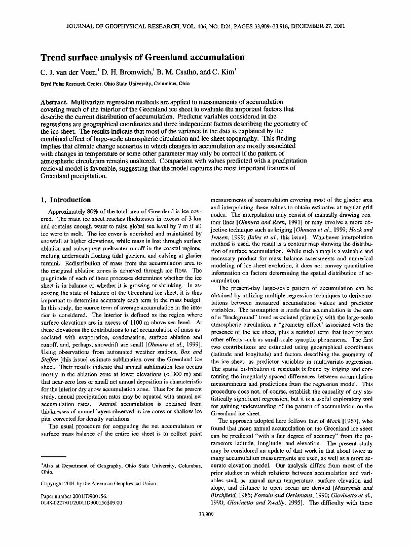
Table 2. Principal Components for Ice Sheet Geometry

Principal Component' Explained Variance, %

PC1 = -2392.094 + 0.987xE- 0.001 xS N + 0.161 xS E

PC2 = 467.881 - 0.158xE + 0.159xS N + 0.975 xS E

PC3 = 103.408 - 0.027xE - 0.987 xS N + 0.157xS E

80.6

12.3

7.1

apc1, PC2, and PC3 are first, second, and third principal components, respectively; E is elevation, measured in meters above sea level; S N and S E are slope in the north and east directions, respectively, measured in meters per kilometer.

dictor in the regression model. The correlation between trend re- sidual and east slope is not significant.

As a start, the geometry effect on accumulation can be found by regressing geographic trend residuals on geometry variables. The geometry of the ice sheet may be characterized by three pa- rmeters, namely, elevation of the ice surface and slopes in the north and east directions. These variables are not independent, however, and therefore cannot be used directly in a regression model. For example, surface slopes generally increase toward the margins where the ice surface is lower. To eliminate correla- tions between the three predictor variables describing ice sheet geometry, three mutually orthogonal principal components are calculated [Hamilton, 1992, chapter 8]. Table 2 gives the factor score coefficients for each component as well as the percent of total variance in the original variables explained by each compo- nent. Note that slopes (in degrees) are multiplied by 1000 so their magnitude (ranging from about -400 to +400) is of the satne order as that of elevations (ranging from --1000 to -3500 m above sea level) and the relative importance of each to the princi- pal components can be inferred from the coefficients in Table 2.

While the third component (PC3) explains the smallest per- centage of variance, it is the component that correlates most sig- nificantly with the geographic trend residuals; a less obvious but, nevertheless, statistically significant correlation exists between geographic trend residuals and the first principal component (PC1) (Figure 4). A formal regression analysis of the geographic trend residual (TR) shows

TR = 0.003 + 0.036 PC3 - 0.004 PC1.

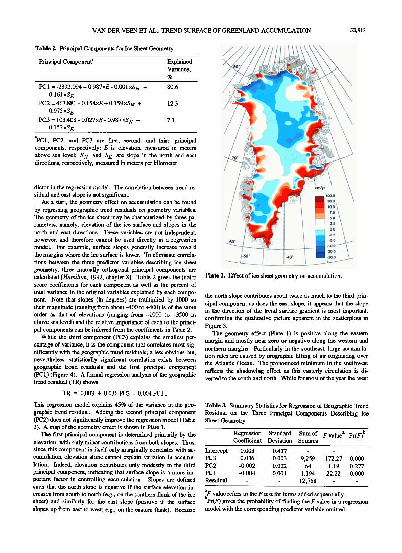
This regression model explains 45% of the variance in the geo- graphic trend residual. Adding the second principal component (PC2) does not significantly improve the regression model (Table 3). A map of the geometry effect is shown in Plate 1.

The first principal component is determined primarily by the elevation, with only minor contributions from both slopes. Thus, since this component in itself only marginally correlates with ac- cumulation, elevation alone cannot explain variation in accumu- lation. Indeed, elevation contributes only modestly to the third principal component, indicating that surface slope is a more im- portant factor in controlling accumulation. Slopes are defined such that the north slope is negative if the surface elevation in- creases from south to north (e.g., on the southern flank of the ice sheet) and similarly for the east slope (positive if the surface slopes up from east to west; e.g., on the eastern flank). Because

Plate 1. Effect of ice sheet geometry on accumulation.

the north slope contributes about twice as much to the third prin- cipal component as does the east slope, it appears that the slope in the direction of the trend surface gradient is most important, confirming the qualitative picture apparent in the scatterplots in Figure 3.

The geometry effect (Plate 1) is positive along the eastern margin and mostly near zero or negative along the western and northern margins. Particularly in the southeast, large accumula- tion rates are caused by orographic lifting of air originating over the Atlantic Ocean. The pronounced minimum in the southwest reflects the shadowing effect as this easterly circulation is di- verted to the south and north. While for most of the year the west

Table 3. Summary Statistics for Regression of Geographic Trend Residual on the Three Principal Components Describing Ice Sheet Geometry

Regression Standard Sum of F value a Pr(F) b Coefficient Deviation Squares

Intercept 0.003 0.437 - - - PC3 0.036 0.003 9,259 172.27 0.000 PC2 -0.002 0.002 64 1.19 0.277

PC 1 -0.004 0.001 1,194 22.22 0.000 Residual - - 12,758 - -

aF value refers to the F test for terms added sequentially. bPr(F) gives the probability of finding the F value in a regression model with the corresponding predictor variable omitted

33,914 VAN DER VEEN ET AL.: TREND SURFACE OF GREENLAND ACCUMULATION

40-

20-

m

-2O

-2000

First principal component

40 b .

20

I % ß

o

-20

-1500 -500 500 1500

Second principal component

40 1 C . 20

-1000 0 1000

Third principal component Figure 4. Scatterplots of geographic trend residuals versus three principal components describing the ice sheet geometry.

coast is subjected to westerly flow from Davis Strait and Baffin Bay, the map in Plate 1 suggests that this circulation does not penetrate sufficiently inland to cause a coastal maximum in ac- cumulation, except in the extreme southwestern portion of the ice sheet and in the region near Thule in the northwest. Both the summer and winter circulation in this region are from the Davis Strait and northward along the western ice sheet margin and are deflected westward as they reach the south facing slope near Thule [Ohmura and Reeh, 1991]. Thus moist air is continuously advected toward this region, resulting in large accumulation as this air is orographically lifted upward on the south facing slope.

It should be noted here that part of the effect of ice sheet to- pography on air flow and thus on accumulation may also be in- cluded in the geographic trend sin'face shown in Figure 2. That map shows generally largest accumulation values along the west- ern margin which may reflect, to some extent, the orographic ef- fect. The geometry effect shown in Plate 1 should be interpreted as a more regional effect, associated with the interaction between surface topography and atmospheric circulation.

The map in Plate 1 shows many small-scale features and ir- regularities caused by small-scale surface topography (variations over tens of kilometers). At several sites in Antarctica a relation between snow accumulation and topography on this scale has been established [Black and Budd, 1964; Whillans, 1975; Van der Veen et al., 1999]. However, such a .."elation has not been found for the Greenland ice sheet, and to do so, observitions along a closely spaced grid in the direction of the prevailing wind would be needed. Interpreting Plate 1 as supporting the model that small-scale topographic features cause fluctuations in accumula- tion rate may be stretching the regression results because of the large spacing between measurement sites. As shown in the bot- tom plot of Figure 4, while there is a significant correlation be- tween the geographic trend residual and the third principal com- ponent of ice sheet geometry, considerable scatter is also evident. Thus the general pattern shown in Plate 1 describes the effect of ice sheet geometry on accumulation, but the small-scale features are likely to be an artifact of the regression model combined with local variations in surface slope.

6. Combined Regression Model

In section 4 the geographic trend surface is derived from mul- tivariate regression of accumulation on geographic coordinates, while in section 5 the geometry effect is estimated by regressing the geographic trend residual on the first and third principal com- ponents characterizing the ice sheet geometry. This is an accept- able procedure for investigating the nature of each effect sepa- rately, but for further analysis of the residual, multivariate regres- sion on all parameters is needed. While it may be expected that the results of a multivariate regression involving both geographic coordinates and geometry factors are broadly similar to the re- sults obtained above, simultaneous regression does not necessar- ily yield the same regression coefficients as obtained from two separate regressions. Nor is it a priori certain that the most sig- nificant regression model is given by the sum of the quadratic trend surface plus the third principal component. It may well be that some of the higher-order terms in the quadratic trend model become insignificant if the principal components are added to the regression model [Draper and Smith, 1998, chapter 12].

The best model can be found using stepwise regression in- cluded in most statistical software packages. In short, this proce- dure starts with a regression equation containing one or two pre- dictor variables and improves on this model by adding or deleting subsequent predictors. Additional predictors are retained if the regression improves significantly (as determined by an F test). After a variable has been added, the regression equation is ex- amined to determine whether any of the other variables should be deleted [cf., Draper and Smith, 1998, pp. 335-336]. Results of this procedure are given in Table 4 and indicate that the large- scale trend explains 80% of the variance in the data (the total sum of squares is 66,565, of which 52,835 is explained by the regres- sion; see Table 4, fourth column). The large-scale trend shown in Plate 2 represents the merger of the trend surface shown in Figure 2 and the geometry effect shown in Plate 1. Most of this pattern

VAN DER VEEN ET AL.' TREND SURFACE OF GREENLAND ACCUMULATION 33,915

Table 4. Summary Statistics of the Co•nbined Accumulation Regression Model

Regression Standard Sum of F value Pr(F) Coefficient Deviation Squares

Intercept 185.911 7.427 - - - Latitude -2.489 0.094 24,710 478.51 0.000 Longitude -0.570 0.064 16,397 330.79 0.000 PC3 0.036 0.024 9,429 190.23 0.000 PC 1 -0.008 0.003 2,299 46.38 0.000 Residual - - 13,730 - -

is explained by the large-scale atmospheric circulation over the ice sheet and orographic forcing near the margins where surface slopes are large [Ohmura and Reeh, 1991]. Again, small-scale variations in accumulation rate are associated with local slopes, as mentioned in section 5.

In determining the large-scale regression surface shown in Plate 2, no data from coastal weather stations were used. Conse- quently, the map may not be entirely realistic near the margins as these values are based on extrapolation of the trend surface out- side the region of data used to derive the regression model. Nev- ertheless, several of the marginal features are supported by other analyses, suggesting that, at least in some places, the large-scale trend captured by the observations in the interior continues far- ther out toward the margins. For exmnple, high accumulation rates along the southwestern and southeastern coasts are also found in the accumulation map of Bales et al. [this issue] and in

Plate 2. Large-scale trend.

the precipitation modeling of Chen et al. [1997]. Shnilarly, the region of high accumulation in the Thule area appears to be a ro- bust feature. On the other hand, there is no corroborating evi- dence for the zone of high accumulation along the central eastern margin of the ice sheet, and it is not clear whether this feature is realistic.

7. Spatial Correlation Kuhns et al. [1997] consider a variety of annual accumulation

measurements to assess the spatial continuity of the signal-to- noise variance ratio. From this ratio the correlation coefficient between records separated by some distance can be derived. This correlation refers to synoptic scale variations in snowfall com- pared with the mean and is thus a measure of the spatial scale of typical precipitation storm systems. In the present study, decadal or longer average values of accumulation rates are considered, necessitating a different approach to estimate the spatial scale of synoptic systems.

A measure of spatial continuity is provided by the omnidirec- tional variogram, ¾, defined through

I N•h) [ Z(si) _ Z(si +h)]2, ¾(h) = 2N(h) i=l in which Z(si) represents the data value at location s i and the summation is over the N(h) data points separated by a distance h [Cressie, 1993, p. 56]. Figure 5 shows estimated variograms (calculated using a lag spacing of 25 km and lag tolerance of half the spacing) for the actual data, t. he large-scale trend surface (shown in Plate 2), and residuals. Also shown in Figure 5 are the corresponding covariograms, C, calculated from

1 7(=•7)•Z(,,)- J •[ Z(' i +h)- •'•, C(h) = N(h) in which the overbar denotes the sample average [Cressie, 1993, p. 56]. The horizontal dashed lines in Figure 5 represent the total variance in the data considered. This variance, equal to the square of the standard deviation, is calculated from

' N-1 n=l

[Davis, 1986, p. 33]. Considering Figure 5a, the increasing value of ¾(h) and de-

creasing C(h) indicate that the spatial correlation gradually de- creases until a separation distance of about 600 km is reached. Over distances greater than -1000 km, accumulation becomes anticorrelated (¾(h) greater than the total variance, C(h) < 0). This phenomenon is associated with the large-scale trend and the accumulation maximum in the south and minimum in the north

(Figure 2). Indeed, the vario•am for the large-scale trend ex- plains most of the spatial correlation, as indicated by the similar- ity between the curves in Figures 5a and 5b. Thus the length scale of the spatially coherent impact of the ice sheet topography on the atmospheric 850-hPa circulation is of the order of 500 km. For the residual the correlation length is -200 km. This finding agrees with the pattern of surface elevation change derived froin satellite radar althnetry, which appears to be coiwelated over dis- tances less than -170 km [Tho,ms et al., 2000], suggesting a spatial con'elation length for major cyclonic precipitation distur- bances of 200 km or less.

33,916 VAN DER VEEN ET AL.: TREND SURFACE OF GREENLAND ACCUMULATION

o

400

200

-200

Accumulation

0 500 1000 1500

400 - b

1,,,,i,,,,i,,,,i 0 500 1000 1500

200 -

•

-200

predictor variables and increases away from this average [Draper and Smith, 1998]. Thus least confidence should be placed in re- sults for the extreme northern and southern reaches of the ice

sheet.

One region noteworthy for the large positive residual is dis- sected by the Exp6dition Glaciologique Intemationale au Groen- land (EGIG) line around 70øN. While the pronounced maximum inland from the west coast is to some extent captured by the ge- ometry effect (Plate 1), the comparatively large residual (Plate 3) indicates that factors other than geometry may contibute to this local maximum in accumul[,tion. Reeh [1989] speculates that this feature may be due to relatively easy access of humid air masses passing through the Disko Bugt area onto the ice sheet.

9. Comparison With Model Predictions

The distribution of accumulation may be compared with re- sults from the precipitation retrieval model described by Chen et al. [1997] that utilizes the equivalent geopotential of Chen and Bromwich [1999], and enhanced by Bromwich et al. [this issue]. This diagnostic approach uses twice-daily operational analyses from the European Centre for Medium-Range Weather Forecasts (ECMWF) to calculate the vertical air motion over the Greenland ice sheet on a 50-km grid. Precipitation rates are derived from the vertical motion and the ECMWF estimates of atmospheric moisture content. Annual precipitation amounts are averaged for 1985 to 1999 and are interpolated from the gn'id locations to the measurement locations using an Arc/Info interpolation routine.

0 I Residual -•00 , , • • i • • , , i , , • • I

0 500 1000 1500

Lag (km) Figure 5. Vafiograms for (a) all data, (b) the large-scale trend surface, and (c) the residuals. Bold lines represent the variance, and thin lines represent the covariance. Horizontal dashed lines indicate the variance of the variable considered.

8. Residuals

Residuals m'e defined as measured accumulation rates minus

those predicted by the combined regression model (Table 4). To construct a contour map of these residuals, values at irregularly spaced measurement sites are interpolated to a regular grid (spacing is 50 km) using kriging with the variogram shown in Figure 5c approximated by a spherical function with range 810 km and sill 51.3 (cm WF_Jyr) 2 (WE is water equivalent); the nug- get is set to 21.69 (cm WF_Jyr) 2. The result is shown in Plate 3 and represents that part of the accumulation distribution that is not explained by the interaction between topography and atmos- pheric circulation as captured by the large-scale trend. Over most of the ice sheet the residual is small, of the order of + 2 cm WE/yr. Differences are largest near the margins of the ice sheet but this may be because there are few data points here to con- strain the regression surface and because these regions represent the boundaries of the study area. Generally, the uncertainty in regression predictions is least in the vicinity of the average of

.:!

e

e

,

e

e

0.0

-2.5

-5.0

-20.0

-70.0

Plate 3. Unexplained residuals of accumulation from the large- scale trend. Dots represent locations of accumulation measurements.

VAN DER VEEN ET AL.' TREND SURFACE OF GREENLAND ACCUMULATION 33,917

A comparison between model-predicted precipitation and ob- servations as well as the predicted large-scale pattern is given in Figure 6. Open circles in the top plot correspond to sites in the southwest where the result of Brotnwich e't al. [this issue] is lo- cally unrealistic. These points are excluded from the following comparison. For the regression of model values, Pmodel, with measured values, Pobs ,the result is

Pmodel = 1.13 + 0.95Pobs , R2 = 0.46. When the model is compared with the predicted large-scale pat- tern, Ppred, however, results are improved and the regression equation is

Pmodel = - 6.40 + 1.20Ppred,

and the coefficient of determination increases to R2= 0.61.

120

IO0

8O

60

40

20

a o

o

o

ß

ß 0 oø•

ß

ß

ß

o o

0 20 40 60 80

Measured (cm WE / yr)

1øø -:l 60

2O

ß

ß ß

ß ß

ß

0 20 40 60 80

Predicted trend (cm WE / yr) Figure 6. Comparison between (top) model-predicted precipitation and accumulation observations and (bottom) the large-scale accumulation distribution (bottom) at the measurement locations.

Thus the precipitation model reasonably captures the large-scale distribution of Greenland accumulation.

It should be noted that the comparison between model predic- tions and observations shown in Figure 6 is based on point val- ues. Such a comparison is stringent, as it requires both the loca- tion and the magnitude of maxima and minima to be predicted correctly. A small spatial shift in the accumulation pattern can significantly deteriorate the correlation.

10. Conclusions

Of the total variance in average Greenland accumulation, -80% can be explained by the large-scale atmospheric circulation and its interaction with the geometry of the ice sheet. This pat- tern is captured by the precipitation retrieval model. The re- maining 20% is attributed to small-scale atmospheric processes and variance in the measurements. The spatial pattern of the re- maining variance is displayed by the residuals in Plate 3. These residuals are uncorrelated over distances exceeding -200 km. This length scale most likely represents the typical penetration distance into Greenland of cyclonic precipitation disturbances that usually remain centered offshore. The two largest positive residuals in Plate 3 occur on the EGIG line and near Thule. The

former maximum has been difficult to reproduce by using the precipitation retrieval model, while the latter feature is well re- produced. The precipitation model also resolves to some extent the negative residuals located between 65 ø and 70øN. Thus the precipitation model shows variable skill in resolving the remain- ing 20% of accumulation variance but is likely penalized by the pointwise nature of the evaluation in Figure 6.

The finding that most of the accumulation distribution can be explained by the large-scale atmospheric circulation and the ge- ometw of the ice sheet has implications for modeling studies that simulate the evolution of the Greenland ice sheet over extended

periods of time [Letr•guilly et al., 1991] or in response to the predicted greenhouse warming over the next few centm•ies [Huy- brechts and de Wolde, 1999]. In these studies, climate forcing is included by multiplying the present-day distribution of accumu- lation with a correction factor that depends on the change in air temperature. The underlying assumption is that changes in ac- cumulation are mostly associated with changes in temperature. The results obtained here indicate that this may only be correct if the pattern of atmospheric circulation remains the same as it is now. This appears unlikely, however. During glacial maxima, large ice sheets covered the North American and Eurasian conti- nents, and these ice sheets, up to 3 km in height, affected the at- mospheric circulation [Kageyanm et al., 1999]. Similarly, green- house warming, if effected, is not expected to be uniform and may result in a shift of dominant low-pressure systems such as the Icelandic Low and the low over Baffin Bay, which determine to a large extent the present-day circulation over the Greenland ice sheet. These changes in air flow may well be significantly more important in determining future and past accumulation rates than changes in air temperature are.

Acknowledgments. This work was supported by NASA through awards NAG5-6001, NAG5-8632, and NAS5-99003 (subcontract G042- 0001). Byrd Polar Research Center contribution number C-1200.

References

Bales, R. C., J. R. McConnell, E. Mosley-Thompson, and B. Csatho, Ac- cumulation on the Greenland ice sheet from historical and recent rec-

ords, J. Geophys. Res., this issue.

33,918 VAN DER VEEN ET AL.: TREND SURFACE OF GREENLAND ACCUMULATION

Bamber, J. L., S. Ekholm, and W. B. Krabill, A new, high-resolution digital elevation model of Greenland fully validated with airborne la- ser altimeter data, J. Geophys. Res., 106, 6733-6745, 2001.

Bender, G., The distribution of snow accumulation on the Greenland ice sheet, M.S. thesis, Univ. of Alaska, Fairbanks, 1984.

Black, H. P., and W. Budd, Accumulation in the region of Wilkes, Wilkes Land, Antarctica, J. Glaciol., 5, 3-15, 1964.

Box, J. E., and K. Steffen, Sublimation on the Greenland ice sheet from automated weather station observations, J. Geophys. Res., this issue.

Bromwich, D. H., Q.-S. Chen, L.-S. Bai, E. N. Cassano, and Y. Li, Modeled precipitation variability over the Greenland ice sheet, J. Geophys. Res., this issue.

Chen, Q.-S., and D. H. Bromwich, An equivalent isobaric geopotential height and its application to synoptic analysis and to a generalized to- equation in c•-coordinates, Mon. Weather Rev., 127, 145-172, 1999.

Chen, Q.-S, D. H. Bromwich, and L. Bai, Precipitation over Greenland retrieved by a dynamic method and its relation to cyclonic activity, J. Clint., 10, 839-870, 1997.

Cressie, N. A. C., Statistics for Spatial Data, (rev. ed.), 900 pp., John Wiley, New York, 1993.

Csatho, B., C. Kim, and J. Bolzan, Development of Greenland GIS data- base system, in PARCA Report 1998, edited by W. Abdalati, NASA/TM-1999-209205, pp. 80-84, Greenbelt, Md, 1999.

Davis, J. C., Statistics and Data Analysis in Geology, 2nd ed., 646 pp., John Wiley, New York, 1986.

Draper, N. R., and H. Smith, Applied Regression Analysis, 3rd ed., 706 pp., John Wiley, New York, 1998.

Fortuin, J.P. F., and J. Oerlemans, Parameterization of the annual sur- face temperature and mass balance of Antarctica, Ann. Glaciol., 14, 78-84, 1990.

Giovinetto, M. B., and H. J. Zwally, Annual changes in sea ice extent and of accumulation on ice sheets: implications for sea level variabil- ity, Z. Gletscherkd. Glazialgeol., 31, 39-49, 1995.

Giovinetto, M. B., N.M. Waters, and C. R. Bentley, Dependence of Ant- arctic surface mass balance on temperature, elevation, and distance to open ocean, J. Geophys. Res., 95, 3517-3531, 1990.

Hamilton, L. C., Regression with Graphics.' A Secorot Course in Applied Statistics, 363 pp., Duxbury, Boston, Mass., 1992.

Hock, R., and H. Jensen, Application of kriging interpolation for glacier mass balance computations, Geogr. Ann. 81(A), 611-619, 1999.

Huybrechts, P., and J. de Wolde, The dynamics response of the Green- !and and Antarctic ice sheets to multiple-century climatic warming, J. Clbn., 12, 2169-2188, 1999.

Isaaks, E. H., and R. M. Srivastava, An Introduction to Applied Geosta- tistics, 561 pp., Oxford Univ. Press, New York, 1989.

Kageyama, M., P. J. Valdes, G. Ramstein, C. Hewitt, and U. Wyputta, Northern Hemisphere storm tracks in present day and last glacial

maximum climate simulations: a comparison of the European PMIP models, J. Clim. 12, 742-760, 1999.

Kim, C., B. Csath6, R. Thomas, and C. J. van der Veen, Studying and monitoring the Greenland ice sheet using GIS techniques, lnt. Arch. Photogramm. Remote Sens., XXXII(B7/2), 678-685, 2000.

Kuhns, H., C. Davidson, J. Dibb, C. Stearns, M. Bergin, and J. -L. Jaf- frezo, Temporal and spatial variability of snow accumulation in cen- tral Greenland, J. Geophys. Res., 102, 30,059-30,068, 1997.

Letr6guilly, A., N. Reeh, and P. Huybrechts, The Greenland ice sheet through the last glacial-interglacial cycle, Palaeogeogr. Palaeocli- matol. Palaeoecol., 90, 385-394, 1991.

Mock, S. J., Accmnulation Patterns on the Greenland Ice Sheet, CRREL Res. Rep. 233, 11 pp., Cold Reg. Res. and Eng. Lab., Hanover N.H., 1967.

Muszynski, I., and G. E. Birchfield, The dependence of Antarctic accu- mulation rates on surface temperature and elevation, Tellus Set'. A, 37, 204-208, 1985.

Ohmura, A., and N. Reeh, New precipitation and accumulation maps for Greenland, J. Glaciol., 3Z 140-148, 1991.

Ohmura, A., P. Calanca, M. Wild, and M. Anklin, Precipitation, accu- mulation and mass balance of the Greenland ice sheet, Z Gletscherkd. Glazialgeol., 35, 1-20, 1999.

Reeh, N., Dynamic and climatic history of the Greenland ice sheet, in Quaternary Geology of Canada and Greenland, Geol. Can., no. 1, edited by R. J. Fulton, pp. 793-822, Geol. Surv. of Can., Ottawa, Ont., 1989.

Thomas, R., T. Akins, B. Csatho, M. Fahnestock, P. Gogineni, C. Kim, and J. Sonntag, Mass balance of the Greenland ice sheet at high ele- vations, Science, 289, 426-428, 2000.

Van der Veen, C. J., E. Mosley-Thompson, A. J. Gow, and B. G. Mark, Accumulation at South Pole: Comparison of two 900-year records, J. Geophys. Res., 104, 31,067-31,076, 1999.

Whillans, I. M., Effect of inversion winds on topographic detail and mass balance on inland ice sheets, J. Glaciol., 14, 85-90, 1975.

Yang, D., S. Ishida, B. E. Goodison, and T. Gunther, Bias correction of daily precipitation measurements for Greenland, J. Geophys. Res., 104, 6171-6181, 1999.

D. H. Bromwich, B. M. Csatho, C. Kim, and C. J. van der Veen, Byrd Polar Research Center, Ohio State University, 108 Scott Hall, 1090 Car- mack Road, Columbus, OH 43210. (bromwich. 1 @osu.edu, csatho. 1 @osu.edu, vanderveen. 1 @osu.edu)

(Received August 28, 2000; revised February 22, 2001; accepted February 28, 2001.)