Traveling Waves - RIT Center for Imaging Science · Chapter 4 Traveling Waves 4.1 Introduction...

Chapter 4

Traveling Waves

4.1 Introduction

To date, we have considered oscillations, i.e., periodic, often harmonic, variations of a physicalcharacteristic of a system. The system at one time is indistinguishable from the system observed ata later time if the time difference is an integral number of temporal periods. To maintain oscillatorybehavior, the energy of the oscillator must remain within the system, i.e., there can be no losses ofenergy. We will now extend this picture to oscillations that travel from the source and thus transportenergy away. Energy must be continually added to the system to maintain the oscillation and thetransported energy can do work on other systems at a distance.Our first task is to mathematically describe a traveling harmonic wave, i.e., denote a y [t] that

travels through space. A harmonic oscillation y(t) = A0 cos(ω0t), can be converted into a travelingwave by making the phase a function of both x and t in a very particular way. Consider the generalcase of an oscillatory function of space and time:

y [z, t] = A0 cos [Φ [z, t]] = A0 cos [z, t] .

We want this oscillation to move through space, e.g., toward positive z. In other words, if a point ofconstant phase on the wave (e.g., a peak of the cosine created at a particular time τ) is at a pointx0 in space at a time t0, the same point of constant phase must move to z1 > z0 at time t1 > t0.

“Snapshots” of sinusoidal wave at two different times t0 and t1 > t0, showing motion of the peakoriginally at the origin at t0. The wave is traveling towards z = +∞ at velocity vφ. The phase of

the first wave at the origin is 0 radians, but that of the second is negative.Since the wave at location z1 and time t1 has the same phase as the wave at location z0 and time

27

28 CHAPTER 4. TRAVELING WAVES

t0, we can say that:

Φ [z0, t0] = Φ [z1, t1] =⇒ cos [z0, t0] = cos [z1, t1] =⇒ y [z0, t0] = y [z1, t1] .

In addition, for the wave to maintain its shape, the phase Φ [x, t] must be a linear function ofx and t; otherwise the wave would compress or stretch out at different locations in space or time.Therefore:

Φ [z, t] = αz + βt

=⇒ αz0 + βt0 = αz1 + βt1.

As discussed, if t1 > t0 =⇒ z1 > z0 (i.e., wave moves toward z = +∞), then α and β must haveopposite algebraic signs:

Φ [z, t] = |α|z − |β|t

By dimensional analysis, we know that |α|z − |β|t has “dimensions” of angle [radians]. We havealready identified β = ω0, the angular frequency of the oscillation. Similarly, if [z] = mm must havedimensions of radians/mm, i.e., α tells how many radians of oscillation exist per unit length — theangular spatial frequency of the wave, commonly denoted by k :

y+ [z, t] = A0 cos [kz − ω0t]− traveling harmonic wave toward z = +∞

By identical analysis, we can derive the equation for a harmonic wave moving toward x = −∞

y− [z, t] = A0 cos [kz + ω0t]− traveling harmonic wave toward z = −∞

The waves are functions of both space and time, i.e., three dimensions [z,y,t] are needed to portraythem. Generally we display y either as a function of z or fixed t, or as a function of t for fixed z :

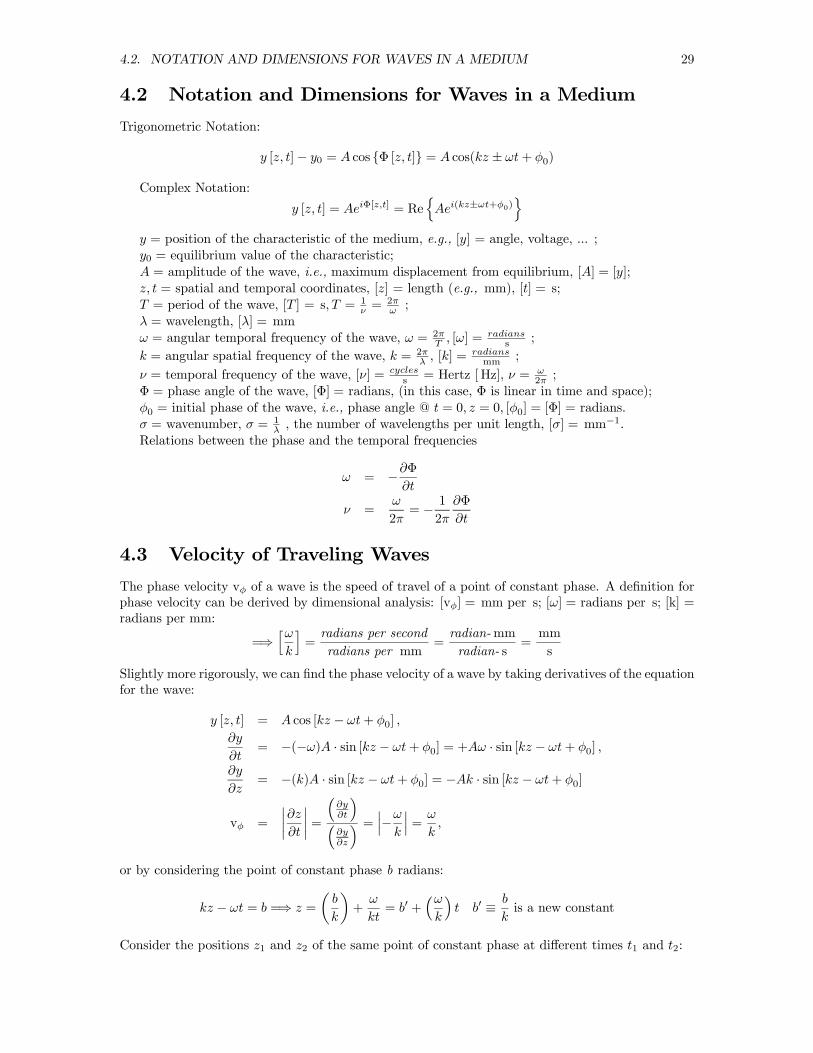
4.1.1 2-D Plot of 1-D Traveling Wave

The 1-D traveling wave is a function of two variables: the position z and the time t, and so maybe graphed on axes with these labels. An example is shown in the figure, where z is plotted on thehorizontal axis and t on the vertical axis. In this case, the point at the origin at t = 0 has a phaseof 0 radians. That point moves in the positive z direction with increasing time, and so is a wave ofthe form

y [z, t] = cos [k0z − ω0t]

The points with the same phase of 0 radians at later times are positioned along the line shown. Thevelocity of this point of constant phase is ∆z∆t , and thus is the reciprocal of the slope of this line.

4.2. NOTATION AND DIMENSIONS FOR WAVES IN A MEDIUM 29

4.2 Notation and Dimensions for Waves in a Medium

Trigonometric Notation:

y [z, t]− y0 = A cos Φ [z, t] = A cos(kz ± ωt+ φ0)

Complex Notation:

y [z, t] = AeiΦ[z,t] = RenAei(kz±ωt+φ0)

oy = position of the characteristic of the medium, e.g., [y] = angle, voltage, ... ;y0 = equilibrium value of the characteristic;A = amplitude of the wave, i.e., maximum displacement from equilibrium, [A] = [y];z, t = spatial and temporal coordinates, [z] = length (e.g., mm), [t] = s;T = period of the wave, [T ] = s, T = 1

ν =2πω ;

λ = wavelength, [λ] = mmω = angular temporal frequency of the wave, ω = 2π

T , [ω] = radianss ;

k = angular spatial frequency of the wave, k = 2πλ , [k] =

radiansmm ;

ν = temporal frequency of the wave, [ν] = cycless = Hertz [ Hz], ν = ω

2π ;Φ = phase angle of the wave, [Φ] = radians, (in this case, Φ is linear in time and space);φ0 = initial phase of the wave, i.e., phase angle @ t = 0, z = 0, [φ0] = [Φ] = radians.σ = wavenumber, σ = 1

λ , the number of wavelengths per unit length, [σ] = mm−1.Relations between the phase and the temporal frequencies

ω = −∂Φ∂t

ν =ω

2π= − 1

2π

∂Φ

∂t

4.3 Velocity of Traveling Waves

The phase velocity vφ of a wave is the speed of travel of a point of constant phase. A definition forphase velocity can be derived by dimensional analysis: [vφ] = mm per s; [ω] = radians per s; [k] =radians per mm:

=⇒hωk

i=radians per secondradians per mm

=radian-mmradian- s

=mm

s

Slightly more rigorously, we can find the phase velocity of a wave by taking derivatives of the equationfor the wave:

y [z, t] = A cos [kz − ωt+ φ0] ,

∂y

∂t= −(−ω)A · sin [kz − ωt+ φ0] = +Aω · sin [kz − ωt+ φ0] ,

∂y

∂z= −(k)A · sin [kz − ωt+ φ0] = −Ak · sin [kz − ωt+ φ0]

vφ =

¯∂z

∂t

¯=

³∂y∂t

´³∂y∂z

´ = ¯−ωk

¯=

ω

k,

or by considering the point of constant phase b radians:

kz − ωt = b =⇒ z =

µb

k

¶+

ω

kt= b0 +

³ωk

´t b0 ≡ b

kis a new constant

Consider the positions z1 and z2 of the same point of constant phase at different times t1 and t2:


z1 = b0 +³ωk

´t1

z2 = b0 +³ωk

´t2

=⇒ z1 − z2 = ∆z =³ωk

´(t1 − t2) =

³ωk

´∆t

vφ ≡ ∆x

∆t=

ω

k= vφ.

4.4 Superposition of Traveling Waves

Consider the superposition of two traveling waves with the same amplitude, different phase velocities,and different frequencies:

y1 [z, t] = A cos [k1z − ω1t]

y2 [z, t] = A cos [k2z − ω2t] .

We can use the same derivation developed for oscillations by defining a new frequency for both:

Ω1 ≡ k1z

t− ω1

Ω2 ≡ k2z

t− ω2

y [z, t] = y1 [z, t] + y2 [z, t] = A cos [k1z − ω1t] + cos [k2z − ω2t]

= A

½cos

∙µk1z

t− ω1

¶t

¸+ cos

∙µk2z

t− ω2

¶t

¸¾= A cos [Ω1t] + cos [Ω2t]

= 2A cos

∙µΩ1 +Ω2

2

¶t

¸cos

∙µΩ1 − Ω2

2

¶t

¸

just as before.By evaluating the sum and difference frequencies, we obtain:

µΩ1 +Ω2

2

¶t =

µk1z

t− ω1 +

k2z

t− ω2

¶t

2=

µk1 + k22

¶z −

µω1 + ω22

¶t ≡ kavgz − ωavgt

where kavg ≡ k1 + k22

, ωavg ≡ω1 + ω22

µΩ1 − Ω2

2

¶t =

µk1z

t− ω1 −

k2z

t+ ω2

¶t

2=

k1 − k22

z − ω1 − ω22

t ≡ kmodz − wmodt

where kmod ≡ k1 − k22

, ωmod ≡ω1 − ω22

4.5. STANDING WAVES 31

4.5 Standing Waves

Consider the superposition of two waves with the same amplitude A0, temporal frequency ν0, andwavelength λ0, but that are traveling in opposite directions:

f1 [z, t] + f2 [z, t] = A0 cos [k0z − ω0t] +A0 cos [k0z + ω0t]

= 2A0 cos

∙k0z − ω0t

2+

k0z + ω0t

2

¸· cos

∙k0z − ω0t

2− k0z + ω0t

2

¸= 2A0 cos

∙k0z + k0z

2+−ω0t+ ω0t

2

¸· cos

∙k0z − k0z

2+−ω0t− ω0t

2

¸= 2A0 cos [k0z] · cos [−ω0t]= 2A0 cos [k0z] · cos [ω0t] , because cos [−θ] = +cos [+θ]

= 2A0 cos

∙2π

z

λ0

¸· cos [2πν0t]

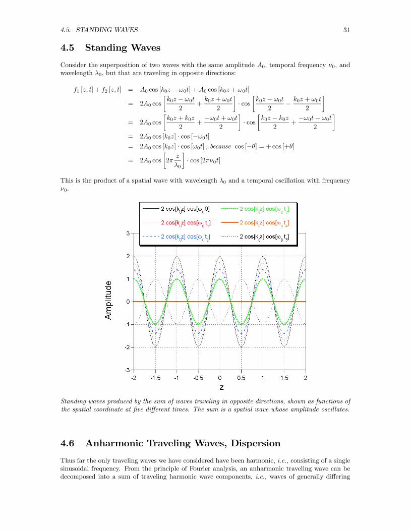
This is the product of a spatial wave with wavelength λ0 and a temporal oscillation with frequencyν0.

Standing waves produced by the sum of waves traveling in opposite directions, shown as functions ofthe spatial coordinate at five different times. The sum is a spatial wave whose amplitude oscillates.

4.6 Anharmonic Traveling Waves, Dispersion

Thus far the only traveling waves we have considered have been harmonic, i.e., consisting of a singlesinusoidal frequency. From the principle of Fourier analysis, an anharmonic traveling wave can bedecomposed into a sum of traveling harmonic wave components, i.e., waves of generally differing


amplitudes over a discrete set of frequencies:

y [z, t] =∞Xn=1

yn =∞Xn=1

An cos [knz − ωnt+ φn] ,

where An, kn, and ωn are the amplitude, angular spatial frequency, and angular spatial frequencyof the nth wave. Therefore, we can define the phase velocity of the nth wave as:

(vφ)n =ωnkn

.

Now suppose that a particular anharmonic oscillation is composed of two harmonic componentsy [x, t] = y1(x, y)+y2 [x, t]. If the two components have the same phase velocity, (vφ)1 = (vφ)2, thenpoints of constant phase on the two waves move with the same speed and maintain the same relativephase. The shape of the resultant wave is invariant over time. Such a wave is called nondispersive,because points of constant phase on the components do not separate over time.What if the phase velocities are different, i.e., if (vφ)1 6= (vφ)2? In this case, points of constant

phase on the two waves will move at different velocities, and therefore the distance between points ofconstant phase will change as a function of position or time. Therefore the shape of the superpositionwave will change as a function of time; these waves are dispersive.Note that the dispersion is a characteristic of the medium within which the waves travel, and

not of the waves themselves. It is the medium that determines the velocities and thus whether thewaves travel together or if they disperse with time and space.

4.7 Average Velocity and Modulation (Group) VelocityWe added two traveling waves of different frequencies and obtained the same result we saw whenadding two oscillations: the sum of two harmonic waves yields the product of two harmonic waveswith modulation and average spatial and temporal frequencies. Using the new terms: kavg, kmod, ωavg,and ωmod, we can define the phase velocities of the average and modulation waves:

vavg ≡ ωavgkavg

=

¡ω1+ω22

¢¡k1+k22

¢ = ω1 + ω2k1 + k2

vmod ≡ ωmodkmod

=

¡ω1−ω22

¢¡k−k22

¢ =ω1 − ω2k1 − k2

These two velocities have the same meaning as the phase velocity of the single wave, i.e., it is thevelocity of a point of constant phase of the average traveling wave frequency or of the modulationwave frequency, or beats wave. The modulation velocity is also commonly called the group velocity .

4.7.1 Example: Nondispersive Waves (vφ)1 = (vφ)2In a nondispersive medium, the phase velocity is constant over frequency (or wavelength), i.e.,

(vφ)1 =ω1k1= (vφ)2 =

ω2k2

.

Note that ω1 6= ω2 and k1 6= k2 — only the ratios are equal. Now find expressions for vmod and vavg.

vavg =ωavgkavg

=ω1+ω22

k1+k22

=ω1 + ω2k1 + k2

=ω1

³1 + ω2

ω1

´k1

³1 + k2

k1

´Since ω1

k1= ω2

k2for nondispersive waves =⇒ ω2

ω1= k2

k1and:

vavg =ω1k1

1 + k2k1

1 + k2k1

=ω1k1= v1 = v2 = vavg .

4.8. DISPERSION RELATION FOR NONDISPERSIVE TRAVELING WAVES 33

Similarly for the velocity of the modulation wave:

vmod =ωmodkmod

=ω1−ω22

k1−k22

=ω1 − ω2k1 − k2

=ω1

³1− ω2

ω1

´k1

³1− k2

k1

´Since ω1

k1= ω2

k2for nondispersive waves, then ω2

ω1= k2

k1and:

vmod =ω1k1

1− k2k1

1− k2k1

=ω1k1= v1 = v2 = vmod = vavg .

Note also that ωmod = ω1−ω2k1−k2 =

∆ω∆k =⇒

dωdk = ωmod

In a nondispersive medium, all waves (all spatial and temporal frequencies and all modulation andaverage waves) travel at the same velocity.

4.8 Dispersion Relation for Nondispersive Traveling Waves

Waves are nondispersive in some important physical cases: e.g., light propagation in a vacuum andaudible sound in air. Since ω

k =vφ, we can easily express the temporal angular frequency ω in termsof the angular wavenumber k:

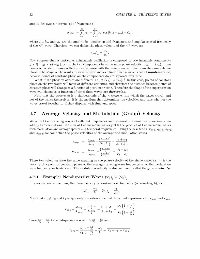
ω = ω(k) = (vφ) · k where vφ is constant, so that ω ∝ k.

The expression of ω in terms of k is called a dispersion relation. We can plot ω [k] vs. k, giving astraight line in the nondispersive case.

Dispersion Relation for Nondispersive Waves, Two types of wave with different velocities(vφ)1 > (vφ)2.

4.9 Dispersive Traveling Waves

The more general, more common, and more important case is that of dispersive waves. Here, thephase velocity vφ = ω

k is not constant; vφ varies with frequency. This is the normal state of affairs


for light traveling in a medium such as glass. The common specification of the phase velocity oflight in medium is the refractive index n:

n =c

vφ

where vφ is the phase velocity of light in the medium. In a dispersive medium, we can interpretgroup velocity in another way:

ω(k) = k · vφ

=⇒ vmod =dω

dk=

d

dk(k · vφ)

=

µdk

dk

¶vφ + k ·

µdvφdk

¶= vφ + k

µdvφdk

¶.

In other words, the group velocity is the sum of the phase velocity vφ and a term proportional todvφdk , which is the change in phase velocity with wavenumber:

dvφdk

> 0 =⇒ vmod > vφ

dvφdk

< 0 =⇒ vmod < vφ.

As the phase velocity varies, the refractive index varies inversely (faster velocity =⇒ smaller index).Variation of the refractive index implies a change in the refractive angle of light entering or exitingthe medium (via Snell’s law). Variation of refractive index with wavelength implies that differentfrequencies will refract at different angles. This is the principle of the dispersing prism.

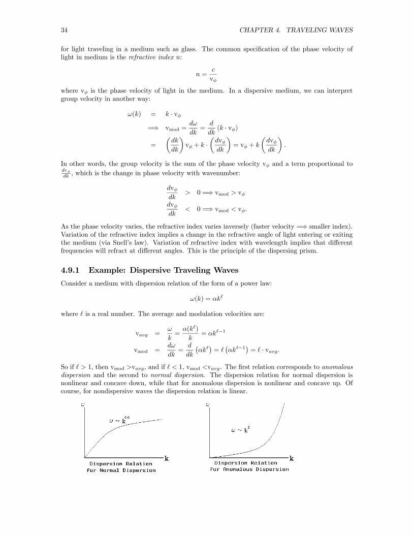
4.9.1 Example: Dispersive Traveling Waves

Consider a medium with dispersion relation of the form of a power law:

ω(k) = αk

where is a real number. The average and modulation velocities are:

vavg =ω

k=

α(k )

k= αk −1

vmod =dω

dk=

d

dk

¡αk

¢=

¡αk −1

¢= · vavg.

So if > 1, then vmod >vavg, and if < 1, vmod <vavg. The first relation corresponds to anomalousdispersion and the second to normal dispersion. The dispersion relation for normal dispersion isnonlinear and concave down, while that for anomalous dispersion is nonlinear and concave up. Ofcourse, for nondispersive waves the dispersion relation is linear.

4.9. DISPERSIVE TRAVELING WAVES 35

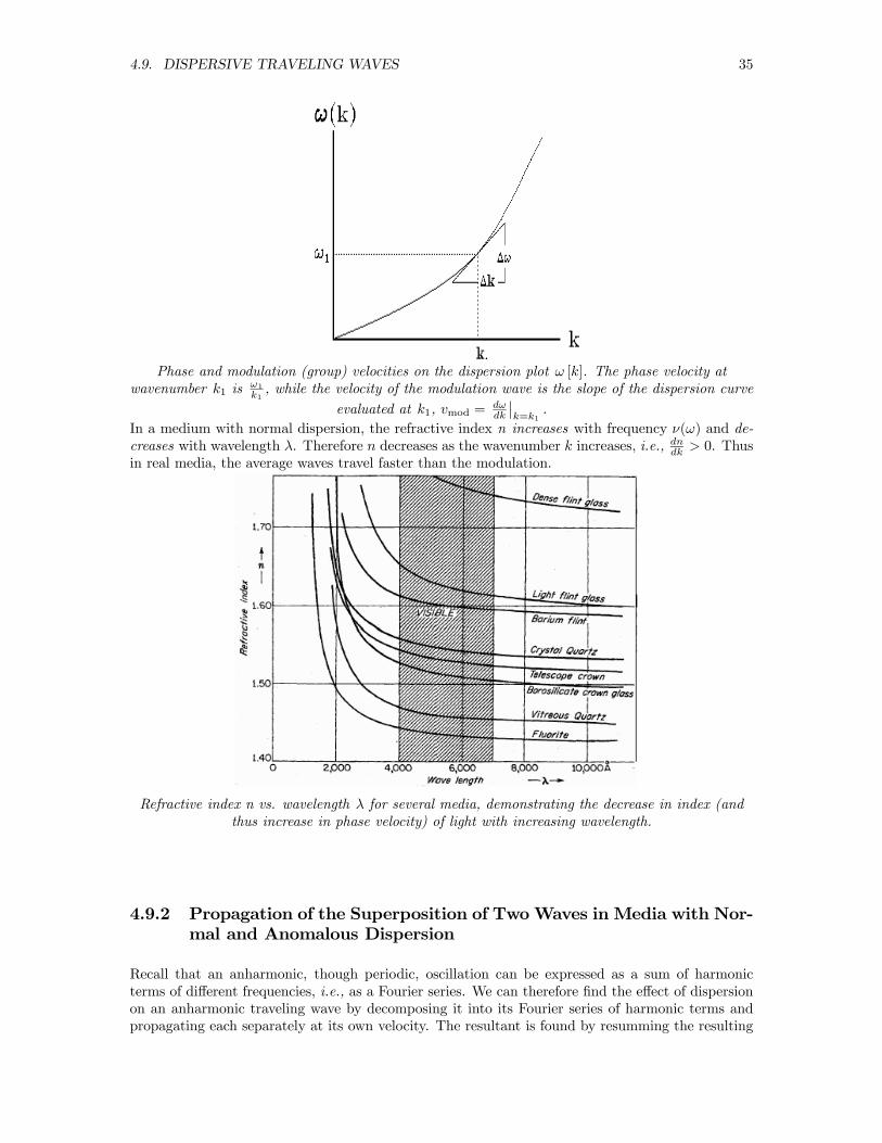
Phase and modulation (group) velocities on the dispersion plot ω [k]. The phase velocity atwavenumber k1 is ω1

k1, while the velocity of the modulation wave is the slope of the dispersion curve

evaluated at k1, vmod = dωdk

¯k=k1

.

In a medium with normal dispersion, the refractive index n increases with frequency ν(ω) and de-creases with wavelength λ. Therefore n decreases as the wavenumber k increases, i.e., dndk > 0. Thusin real media, the average waves travel faster than the modulation.

Refractive index n vs. wavelength λ for several media, demonstrating the decrease in index (andthus increase in phase velocity) of light with increasing wavelength.

4.9.2 Propagation of the Superposition of TwoWaves in Media with Nor-mal and Anomalous Dispersion

Recall that an anharmonic, though periodic, oscillation can be expressed as a sum of harmonicterms of different frequencies, i.e., as a Fourier series. We can therefore find the effect of dispersionon an anharmonic traveling wave by decomposing it into its Fourier series of harmonic terms andpropagating each separately at its own velocity. The resultant is found by resumming the resulting


components. For example, if:

f [z, t] = A1 sin [k1z − ω1t] +A13sin [k2z − 3ω1t] +

A15sin [k3z − 5ω1t]

As we’ve already seen, f [z, t] is the sum of the first three terms of a square wave. In the nondispersivecase, k2 = 3k1 and k3 = 5k1, and v1 =v2 =v3. The wave at the source is shown below:

In dispersive media, v1 6= v2 6=v3, and the relative phase of the three components will vary asthe wave travels through space. Therefore the resultant wave will become increasingly distorted.

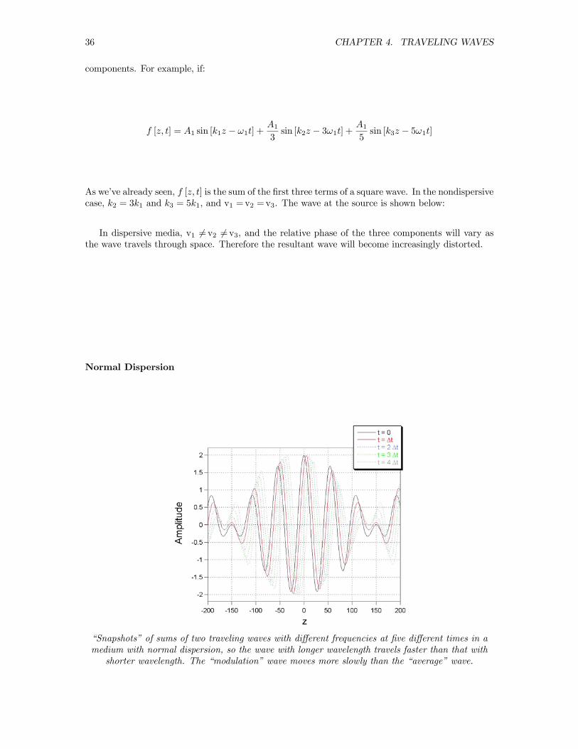
Normal Dispersion

“Snapshots” of sums of two traveling waves with different frequencies at five different times in amedium with normal dispersion, so the wave with longer wavelength travels faster than that with

shorter wavelength. The “modulation” wave moves more slowly than the “average” wave.

4.9. DISPERSIVE TRAVELING WAVES 37

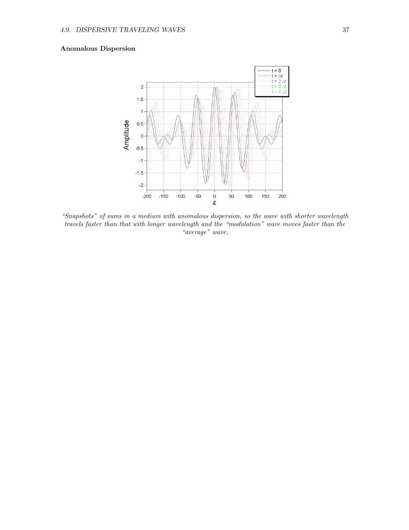
Anomalous Dispersion

“Snapshots” of sums in a medium with anomalous dispersion, so the wave with shorter wavelengthtravels faster than that with longer wavelength and the “modulation” wave moves faster than the

“average” wave.

Traveling Waves - RIT Center for Imaging Science · Chapter 4 Traveling Waves 4.1 Introduction...

Documents

Transcript of Traveling Waves - RIT Center for Imaging Science · Chapter 4 Traveling Waves 4.1 Introduction...