Comput GeosciDOI 10.1007/s10596-006-9030-x

Traveling waves in a finite condensation ratemodel for steam injection

J. Bruining · C.J. van Duijn

Received: 24 May 2005 / Accepted: 25 August 2006© Springer Science + Business Media B.V. 2006

Abstract Steam drive recovery of oil is an economicalway of producing oil even in times of low oil pricesand is used worldwide. This paper focuses on the one-dimensional setting, where steam is injected into a coreinitially containing oil and connate water while oil andwater are produced at the other end. A three-phase(oil, water, steam) hot zone develops, which is abruptlyseparated from the two-phase (oil + water) cold zoneby the steam condensation front. The oil, water andenergy balance equations (Rankine–Hugoniot condi-tions) cannot uniquely solve the system of equationsat the steam condensation front. In a previous study,we showed that two additional constraints follow froman analysis of the traveling wave equation representingthe shock; however, within the shock, we assumed localthermodynamic equilibrium. Here we extend the pre-vious study and include finite condensation rates; usingthat appropriate scaling requires that the Peclet num-ber and the Damkohler number are of the same orderof magnitude. We give a numerical proof, using a color-coding technique, that, given the capillary diffusion be-havior and the rate equation, a unique solution can beobtained. It is proven analytically that the solution forlarge condensation rates tends to the solution obtainedassuming local thermodynamic equilibrium. Computa-

J. Bruining (B)Dietz Laboratory, Centre for Technical Geoscience,Delft University of Technology, Delft, The Netherlandse-mail: j.bruining@ta.tudelft.nl

C.J. van DuijnDepartment of Mathematics and Computer Science,Eindhoven University of Technology,Eindhoven, The Netherlandse-mail: c.j.v.Duijn@tue.nl

tions with realistic values to describe the viscous andcapillary effects show that the condensation rate canhave a significant effect on the global saturation pro-file, e.g. the oil saturation just upstream of the steamcondensation front.

Keywords finite condensation · steam injection ·traveling wave equation

1 Introduction

Steam injection, as a method for enhanced oil recovery,received considerable attention in the petroleum engi-neering literature during the past decades [11, 16, 32].Recently, there is renewed interest for the purpose ofremoving oil spills from the subsurface [3, 19, 20, 23,37, 38]. The processes involved are extremely com-plex and pose challenging questions concerning theory[12, 26, 45, 46], experiment [13, 24, 43] and numericalmodeling [1, 5, 8, 11, 29–31].

The theoretical study described in this paper buildson previous work [7, 39]. In [7], we considered a sim-plified model describing oil recovery by steam drive.The proposed model assumes small capillary forcesand instantaneous condensation as a result of thermo-dynamic equilibrium. It has an upstream hot three-phase (oil, water, steam) flow zone and a downstreamcold two-phase (oil, water) flow zone. The upstreamand downstream zones are separated by a relativelythin transition region, which is described by a (local)steam condensation/capillary diffusion model based onthe ideas of Udell et al. [28, 40, 42]. In the limit ofzero capillary forces, the transition region collapses toform a steam condensation front (SCF). Disregarding

Comput Geosci

capillary pressure away from the condensation front, a2 × 2 hyperbolic system [14, 15] arises for water andsteam. This system cannot be solved uniquely withoutadditional conditions at the SCF. To find these condi-tions, we studied traveling waves of the capillary modelin the transition region [21, 22, 25, 27]. In [7], we investi-gated the effect of different capillary pressure behavior,the effect of gradual-versus-abrupt temperature declinefrom the steam temperature to ambient temperatureand the effect of non-zero gas saturation at the SCF.In all these cases, we assumed local thermodynamicequilibrium. We found and made explicit that detailsof the transition model affect the global behavior of thesteam displacement process. It is therefore of interestto investigate whether the global behavior also dependson the rate constant, i.e. if we drop the assumption ofthermodynamic equilibrium and implement a conden-sation rate model. A finite reaction rate model is alsopreferred in numerical simulations. We expect that inthe limit of large rate constants, the results for localequilibrium are retrieved. The aim of this paper is toinvestigate those two aspects.

In Section 2, we briefly describe the model and re-call the model equations. The hyperbolic setting anda summary of previous results are given in Section 3.In Section 4, we define the traveling wave problemand the method to obtain the unique solution for agiven condensation model. The route to thermody-namic equilibrium is explained in Section 5 by sendingthe rate constant to infinity. We end in Section 6 withcomputations for some realistic cases and comparisonto previous results.

2 Finite rate condensation model

2.1 Physical considerations

Oil displacement by steam drive through a porousmedium is a complex physical process that is controlledby the steam condensation process and by viscous andcapillary forces (see for instance Stewart & Udell [40]and Wingard & Orr [44]. Following ideas of Shutler[39], we proposed in [7] a one-dimensional modelwhere all complexity is confined to a small transitionregion in which the condensation occurs and capillaryforces act. The model describes the case of injectingsteam in a linear core originally filled with oil andconnate water. The porosity ϕ and permeability k areconstant. We allow for temperature-dependent liquidviscosities except that we assume the steam viscosityto be independent of temperature because these vis-cosities are small anyway and the temperature depen-

dence of μg~T0.6 is much smaller than for the liquid

viscosities.The core is horizontal and we disregard the effects of

gravity. Transverse capillary pressure diffusion is suffi-ciently large to guarantee a uniform saturation over thecross-section. The core is positioned along the positivex-axis with flow from left to right, implying that allvariables are functions of position x and time t. The dis-placement is considered to occur at constant pressure,in the sense that we disregard flow-induced pressuregradient effects on the thermodynamic properties, re-action rates, fluid densities and viscosities. Therefore,the pressure does not explicitly enter in the modelequations, but it determines the value of some parame-ters. The temperature dependence of the parameters issummarized in table 1. The oil considered is dead oil;that is, it does not occur in the gas phase. Dissolutionof liquid oil in water and vice versa is disregarded.The condensation occurs between an upstream three-phase flow zone at steam temperature Tb, where oil,water and steam are present, and a downstream two-phase flow zone at the initial reservoir temperature To,where water and oil are present. In the upstream anddownstream regions, capillary forces are disregarded.Consequently, these regions are adequately describedby an (extended) Buckley–Leverett approach. We usepower-law relative permeabilities (both quadratic andfourth powers), as well as Stone I expressions [9].

All condensation occurs in a thin region called thesteam condensation front (SCF). The constant travelspeed of the SCF is determined from an energy balancethat is decoupled from the mass balance equations. Thedecoupling is achieved by disregarding the effect offluid content on the heat capacity (ρc)r of the porousmedium. The velocity vst is determined from a localheat balance, in which the heat released by the condens-ing steam impinging on the SCF is equal to the amountof heat necessary to warm up the reservoir (see Mandland Volek [26]). The result is

vst = ρg�H uinj

(ρc)r(Tb − To).

The symbols appearing in this expression are explainedin table 1.

Within the transition region, there is an interplaybetween viscous forces, capillary forces and the con-densation process. In this paper, we use a finite ratecondensation model. There are three dimensionlessnumbers involved in the processes that occur in thetransition zone, i.e. the Peclet number for mass trans-port (Pe), the Peclet number for heat transport (PeT)and the Damkohler number (Da). These numbers in-dicate the ratio of phase transport by convection and

Comput Geosci

Table 1 Summary of physical input parametersa.

Physical quantity Symbol Value Unit

Characteristic length L 100 mSteam temperature Tb 486 KReservoir temperature To 313 KInjection rate steam uinj 9.52 × 10−4 m3/ m2/ sSteam viscosity μg 1.63 × 10−5 Pa sOil viscosity at Tb μo(Tb) 2.45 × 10−3 Pa sOil viscosity at To μo(To) 0.180 Pa sWater viscosity at Tb μw(Tb) 1.30 × 10−4 Pa sWater viscosity at To μw(To) 7.21 × 10−4 Pa sReference viscosity μ∗

w 5.0 × 10−4 Pa sBrooks–Corey sorting factor λs 2 –Rate constant qb 103 s−1

Enthalpy H2O(l)(To) → H2O(g)(T1) �H 2, 636 kJ/kgEffective heat capacity of rock (ρc)r 2, 029 kJ/m3/KThermal coefficient α 0.017 –Capillary diffusion constant D 1.85 × 10−7 m2/sDiffusion correction factor d 10−2 –Velocity SCF vst 7.12 × 10−5 m/sPorosity ϕ 0.38 m3/m3

Permeability k 1.0 × 10−12 m2

Interfacial tension σ 0.03 N/mWater density ρw 1, 000 kg/m3

Steam density ρg 10.2 kg/m3

Connate water saturation Swc 0.15 m3/m3

Residual gas saturation Sgr 0.0 m3/m3

Residual oil saturation Sor 0.0 m3/m3

a The values of the steam parameters in the table assume a steam pressure of 20 bars. Furthermore, the value of the thermal coefficientα is based on a thermal diffusivity of 9.85×10−7 (m2 /s). Note that this coefficient is proportional to the ratio of the capillary and thermaldiffusivity.

diffusion, the ratio of heat convection and thermal con-ductivity and the ratio of the rate of convected phasetransport and the condensation rate, respectively. Inthe model, we assume an instantaneous temperaturedrop from steam temperature to reservoir temperatureas the steam saturation becomes zero. Furthermore, weassume that the Damkohler number Da and the Pecletnumber Pe are of the same order of magnitude. Wecompare our results to those obtained in [7], whereit was assumed that all steam condenses at a singlepoint in the transition region, the actual (SCF). Therate of condensation is sufficiently fast so that, indeed,all condensation occurs in a small neighborhood of theSCF. Here “small” must be understood in a suitabledimensionless context. In the condensation zone, thetemperature drops from steam temperature Tb to theoriginal reservoir temperature To, and steam condensesat a rate proportional to (Tb − T) , where T is theprevailing temperature. As long as there is steam, thecondensation rate is proportional to the saturation Sg.When the steam saturation is zero, the pores are fullysaturated with water and oil, and the condensation rate

becomes zero. This leads to the following expression forthe mass condensation rate q

q=⎧⎨

⎩

ρgqbTb − TTb − To

Sg for T ≤Tb , 0< Sg ≤1 − Swc,

0 otherwise,(1)

where qb is the condensation rate parameter. As in[7], we assume that the temperature distribution canbe determined independently from the condensationprocess. In fact, in [7], we distinguished between an ex-ponential decline and a stepwise decline. In this paper,we confine ourselves to the stepwise decline. Hence, thetemperature is discontinuous and is given by

T ={

Tb x < vstt,To x ≥ vstt.

The phase densities ρα

(α = w,o,g

)are assumed to be

constant throughout this paper.

Comput Geosci

2.2 Model equations

The mass balance equations for water, steam and oilread{

ϕ∂(ρwSw)

∂t+ ∂(ρwuw)

∂x= q, (2)

{

ϕ∂(ρgSg)

∂t+ ∂(ρgug)

∂x= −q, (3)

{

ϕ∂(ρoSo)

∂t+ ∂(ρouo)

∂x= 0. (4)

where q is given by expression (1). The phase satura-tions satisfy

0 ≤ Swc ≤ Sw ≤ 1, 0 ≤ Sg, So ≤ 1 − Swc. (5)

In other words, we assume that there is no residualoil and gas in the system. We use Darcy’s law for multi-phase flow to express all phase velocities uα in terms ofthe total velocity u and the capillary pressures (see [1]and also [10, 18, 33, 34]. This gives{

uw = ufw + λo fw∂pc,ow

∂x+ λg fw

∂pc,gw

∂x, (6)

{

ug = ufg − λo fg∂pc,go

∂x− λw fg

∂pc,gw

∂x, (7)

{

uo = ufo − λw fo∂pc,ow

∂x+ λg fo

∂pc,go

∂x. (8)

Here

u = uw + uo + ug, (9)

pc,αβ is the capillary pressure, being the pressure dif-ference between phase α and phase β, and fα is thefractional flow function

fα = λα

λo + λw + λg. (10)

Further, λα denotes the mobility of phase α, given by

λα = kkra

μα

,

where krα is the relative permeability (fourth power ofthe effective saturations) and μα is the phase viscosity.Because water and oil experience different tempera-tures, their viscosities may vary significantly across theSCF. Realistic values [4, 35, 41] are given in table 1.In later sections, we use the notation f ±

α , where f −α

denotes the fractional flow function in the hot steamzone and f +

α in the cold oil zone.Because

∑

α

Sα =∑

α

fα = 1 and u =∑

α

uα,

we can eliminate, for instance, So from the equations.Further, summing Eqs. (6), (7) and (8) and usingEq. (9), we find

∂u∂x

=− 1

ρg

(

1− ρg

ρw

)

q=−qb

(

1− ρg

ρw

) (Tb−TTb−To

)

Sg.

(11)

Thus, our primary variables are u, Sw and Sg forwhich we have Eqs. (11), (2+6) and (3+7). Injectingonly steam from the left at x = 0 and having only oiland connate water present at t = 0 require the bound-ary/initial conditions:

u (0, t)=uinj, Sw (0, t)= Swc, and Sg (0, t)=1 − Swc,

(12)

for all t > 0 and

Sw (x, 0) = Swc and Sg (x, 0) = 0, (13)

for all x > 0. In (12), uinj denotes the injection velocityof the steam.

We want to write the Darcy velocities uw and ug interms of capillary diffusion involving Sw and Sg only.For this purpose, we note that

pc,gw = pg − pw = pc,go + pc,ow,

where pc,ow = pc,ow (Sw) is a strictly decreasing functionof the water saturation and where pc,go = pc,ow

(1 − Sg

)

is a strictly increasing function of the gas saturation.For instance, in [7], we considered the Brooks–Coreyexpression (see also [2, 6, 36]),

pc,ow = σ

2

√ϕ

k

(12 − Swc

1 − Swc

)1/λs (Sw − Swc

1 − Swc

)−1/λs

, (14)

where λs > 0 is the sorting factor.Using these observations, we obtain

uw = ufw − Dww∂Sw

∂x− Dwg

∂Sg

∂x, (15)

ug = ufg − Dgw∂Sw

∂x− Dgg

∂Sg

∂x, (16)

where

Dww = − (λo + λg

)fw

dpc,ow

dSw> 0,

Dwg = −λg fwdpc,go

dSg< 0,

Dgw = λw fgdpc,ow

dSw< 0,

Dgg = (λo + λw) fgdpc,go

dSg> 0. (17)

Comput Geosci

Except in Section 6, where we work out a realisticcase based on expression (14), we consider throughoutthis paper

Dww = Dgg = D = constant,

Dwg = Dgw = 0,

where the constant diffusivity is given by

D = σ√

ϕkμ∗

wd.

Here μ∗w denotes a characteristic water viscosity, e.g.

μw (To) and d accounts for the effect of the waterrelative permeability and the functional relation of thecapillary pressure.

2.3 Rescaled equations

We rewrite the equations in dimensionless form bysetting

Sw := Sw − Swc

1 − Swc, So := So

1 − Swc, Sg := Sg

1 − Swc, (18)

T := T − To

Tb − To, u := u

uinj, x := x

L, t := uinjt

ϕL, (19)

where L represents a characteristic length of the prob-lem, for instance, the distance between injection andproduction point. Introducing the reciprocal Pecletnumber ε := D/

(uinjL

)and the dimensionless rate con-

stant r := qbD/u2inj, we find

∂u∂x

= − rε

(1 − α) (1 − T)Sg, (20)

∂Sw

∂t+ ∂ufw

∂x= α

rε(1 − T)Sg + ε

∂2Sw

∂x2, (21)

∂Sg

∂t+ ∂ufg

∂x= − r

ε(1 − T)Sg + ε

∂2Sg

∂x2. (22)

Here α = ρg/ρw. Generally, α << 1. The boundary andinitial conditions follow from (12) and (13). They read

u (0, t) = 1, Sw (0, t) = 0 , Sg (0, t) = 1 for all t > 0

(23)

and

Sw (x, 0) = Sg (x, 0) = 0 for all x > 0. (24)

The scaled temperature T = T (x, t) is discontinuousat the SCF with

T ={

1 x < vt,0 x ≥ vt,

(25)

where v = vst/uinj.

Remark 2.1 Direct scaling of Eq. (11) gives

∂u∂x

= −qbLuinj

(1 − α) (1 − T)Sg

with qb Luinj

being the dimensionless rate parameter(Damkohler number). To balance terms in the equa-tions, in particular after the additional blow-up x :=x/ε, we need

qbLuinj

= rε, with r = O (1) as ε ↓ 0.

Realistic numbers from table 1 give:

qbLuinj

∼ 108, r ∼ 102 and ε ∼ 10−6.

3 Hyperbolic setting and previous results

When the scale L of the problem is such that D <<

uinjL, and thus ε << 1, one expects that Eqs. (20)–(22) reduce to a hyperbolic system, similar to the onestudied in [7], in which all steam condenses at the SCF,i.e.

∂u∂x

= − (1 − α) �δ(x − vt), (26)

∂Sw

∂t+ ∂ufw

∂x= α�δ(x − vt) , (27)

∂Sg

∂t+ ∂ufg

∂x= −�δ(x − vt) . (28)

Here � is the condensation rate that originates fromthe condensation terms in Eqs. (20)–(22) and δ theDirac measure at x = vt. Below we make this precisefor traveling wave solutions.

In [7], we showed that a solution of the system(26)–(28), satisfying (23) and (24) can only be a fastrarefaction with u = 1 in the steam region {x < vt } ,

with a shock at the SCF {x = vt } , and with two-phaseBuckley–Leverett behavior in the cold region {x > vt }where Sg = 0 (see figure 1).

We also showed that to obtain a uniquely con-structed solution, a local transition model at the SCFmust be introduced. In the hyperbolic setting, there arefour unknowns at the SCF: the water and gas saturation(

S−w, S−

g

)on the left, and the water saturation S+

w and

Darcy velocity u+ on the right. Counting the number ofequations between them, we have from mass conserva-tion two Rankine–Hugoniot conditions

(RH)

{f −w − vS−

w + α� = u+ f +w − vS+

w,

f −g − vS−

g − � = 0,(29)

Comput Geosci

Figure 1 Water and gas saturations in hyperbolic model [(26)–(28)]. (a) Saturations in the (x, t) plane with unknowns(

S−w , S−

g , S+w , u+

)

at the steam condensation front. (b) The saturation path in the(Sw, Sg

)plane.

with � = (1 − u+)

/ (1 − α) . A third equation followsfrom the condition that the fast rarefaction has to matchup with the velocity of the SCF. This gives the entropycondition

(E) λ2

(S−

w, S−g

)= v, (30)

where λ2 denotes the largest eigenvalue at(

S−w, S−

g

)of

the Jacobian matrix of the saturation flux(

fw, fg). The

missing fourth relation follows from a traveling waveanalysis of the transition model. In fact, the existencecondition for a traveling wave, giving the shock itsviscous profile, enabled us to construct a unique shocksolution. We considered several local transition models,all having instantaneous condensation, and investigatedtheir influence on the global solution through the shockcondition at the SCF.

The main purpose of this paper is to understandthe finite rate condensation model proposed in Section2. We do this by analyzing traveling wave solutionsof Eqs. (20)–(22). Such solutions allow us to quantifythe role of the rate parameter r and can be used as abuilding block in the construction of a unique shocksolution.

In the finite rate condensation model, the rate con-stant is r/ε, where r = O (1) and ε is small. This ischosen to balance terms in the equations. To see this,we set

η = x − vtε

(31)

and consider the waves

Si = Si (η)(i = w, g

)and u = u (η) . (32)

Because of Eq. (25), we have T = 1 − H (η) , where Hdenotes the Heaviside function

H (η) ={

0 η < 01 η > 0

Substitution of Eqs. (31) and (32) into Eqs. (20)–(22)results in the system of ordinary differential equations

u′ = − (1 − α) r (1 − T) Sg,

−vS′w + (ufw)

′ = αr (1 − T) Sg + S′′w,

−vS′g + (

ufg)′ = −r (1 − T) Sg + S′′

g,

⎫⎬

⎭(33)

where the primes denote differentiation with respect toη. Note that ε has disappeared from the formulationand that the domain of the equations, for ε ↓ 0, rangesfrom η → −∞ to η → +∞. As in [7] we impose theboundary conditions

(BC)

{Sw (−∞) = S−

w, Sg (−∞) = S−g , u (−∞) = 1

Sw (∞) = S+w, Sg (∞) = S+

g , u (∞) = u+

that satisfy (RH) , with � appropriately chosen, and(E) .

Suppose, for the moment, that a traveling wave existsand that the decay of Sg (η) → 0 as η → ∞ is such that

∞∫

0

Sg (η) dη < ∞ (34)

and

limε↓0

1

εSg

(δ

ε

)

= 0 for every δ > 0. (35)

Comput Geosci

Clearly, for i = w,g,

Sεi (x, t) = Si

(x − vt

ε

)

and uε (x, t) = u(

x − vtε

)

are solutions of Eqs. (20)–(22). In these equations, thecondensation terms satisfy for any t > 0

rε

∫

R

(1 − T (x, t)) Sεg (x, t) dx =

rε

∞∫

vt

Sεg (x, t) dx = r

∞∫

0

Sg (η) dη

for all ε > 0, and

limε↓0

rε

(1 − T (x, t)) Sεg (x, t) = 0 for all x = vt.

Hence

limε↓0

rε

(1 − T (x, t)) Sεg (x, t) = �δ (x − vt) ,

where

� = �(r) := r

∞∫

0

Sg (η) dη. (36)

Remark 3.1 Conditions (34) and (35) follow directlyfrom the construction of a solution. In Section 4, weshow that in the

(u, Sw, Sg

)-space, the boundary point(

u+, S+w, 0

)is a saddle with two positive and one nega-

tive eigenvalues. The latter provides exponential decayfrom which Eqs. (34) and (35) directly follow.

In the saturation equations from Eq. (33), wesubstitute

r (1 − T) Sg = − 1

(1 − α)u′.

Integrating the resulting expressions gives

(TW)

⎧⎪⎨

⎪⎩

u′ = − (1 − α) r (1 − T) Sg,

S′w = ufw − vSw + α

1−αu − (

f −w − vS−

w + α1−α

),

S′g = ufg − vSg − 1

1−αu −

(f −g − vS−

g − 11−α

),

with −∞ < η < ∞ .We analyze this dynamical system in the next section.

To emphasize the construction and to avoid technicaldetails, we consider the rather academic case in whichthe viscosities do not depend on temperature and inwhich the viscosity ratios are unity. Taking in addition

quadratic relative permeabilities, the fractional flowfunctions simplify to

fi = fi(Sw, Sg

) = S2i

S2w + S2

g + (1 − Sw − Sg

)2 (37)

and

f ±i = fi

(S±

w, S±g

). (38)

The results for a realistic case, with temperature-dependent viscosities, a large viscosity contrast anddifferent relative permeabilities, will be presented anddiscussed in Section 6.

4 Construction of shocks by means of traveling waves

In this section, we explain the construction of aunique solution satisfying the simplified dynamic sys-tem (TW) , with fractional flow functions given byEqs. (37) and (38), subject to boundary conditions (BC)

satisfying the constraints of Rankine–Hugoniot (RH)

and entropy (E) . The construction uses a shootingargument in the three-dimensional

(u, Sw, Sg

)-space.

Because

Sw + Sg = 1 − So ≤ 1 and u′ ≤ 0,

we expect that a solution is confined to the domain

R = [u+, 1

] × T

where T denotes the saturation triangle

T = {(Sw, Sg

) : Sw, Sg ≥ 0 and Sw + Sg ≤ 1}

As in [7], the solution of the hyperbolic system (26)–(28), satisfying boundary and initial conditions (23 and24), respectively, follows a path as AE in R. This is

Figure 2 Orbit in(u, Sw, Sg

)space.

Comput Geosci

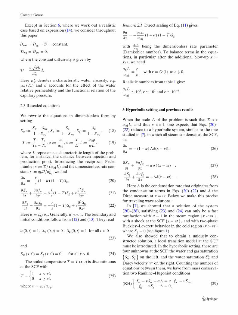
sketched in figure 2. Here A denotes the boundary con-dition (1, 0, 1) . The part AB reflects the fast rarefactionin the steam region where T = 1 and thus u = 1. The

point B =(

1, S−w, S−

g

)∈ l, where

l = {(u, Sw, Sg

) : u = 1 and λ2(Sw, Sg

) = v}

Thus, for points in l, the speed of the fast rarefactionand the SCF coincide. With respect to the two-dimensional triangle {u = 1} × T, the point B is a non-

hyperbolic saddle with eigenvalues(

at(

S−w, S−

g

)of the

Jacobian matrix of the vector(

fw − vSw, fg − vSg) )

e1 < e2 = λ2 − v = 0.

The part BCD reflects the traveling wave as theviscous profile of the shock from B to D = (

u+, S+w, 0

).

Because T (η) = 1 for η < 0, the part of the travel-ing wave with −∞ < η < 0 has u = 1 and is thereforeconfined to the face triangle {u = 1} × T. At C, thetemperature drops from boiling point to reservoir tem-perature implying that T (η) = 0 for η > 0. The pathor orbit representing the solution now moves into thedomain R with strictly decreasing u. At D, all steamhas condensed. A two-phase Buckley–Leverett finallyconnects D to the initial condition E = (

u+, 0, 0), with

only movable oil being present.The aim is now to show that for given α ∈ (0, 1) and

v, r > 0, being the only parameters in the simplifiedproblem, there exists a unique solution of (TW) whichflows from B ∈ l as η → −∞, through C at η = 0, toD as η → ∞. In this solution, B and D are related byconditions (RH) .

We first consider the construction for η < 0. Becauseu (η) = 1 for all η < 0, we drop u from the notation.With reference to figure 3, let Smax

w denote the max-imum water saturation for which

(Sw, Sg

) ∈ l in thesaturation triangle T. For N ∈ N sufficiently large, let

S−w (n) = n

NSmax

w n = 0, 1, 2, ...N , (39)

denote a uniform partition of the interval[0, Smax

w

]and

let B (n) :=(

S−w (n) , S−

g (n))

denote the correspondingpartition of l. For each n ∈ {0, 1, ...N}, we determine atB (n) the eigenvector −→e 2 corresponding to the eigen-value e2 = 0. This vector is indicated in figure 3. In itsdirection, we solve the two saturation equations from(TW) with u = 1 kept fixed. The corresponding solutionis represented by the orbit � (n) in figure 3. It reaches(Sw = S0

w (n) , Sg = 0)

at finite η. Later on, we shallredefine η such that η = 0 corresponds to point C infigure 2.

Figure 3 Construction of solution for η < 0, with u = 1. Here

B (n) denotes the point(

S−w (n) , S−

g (n))

.

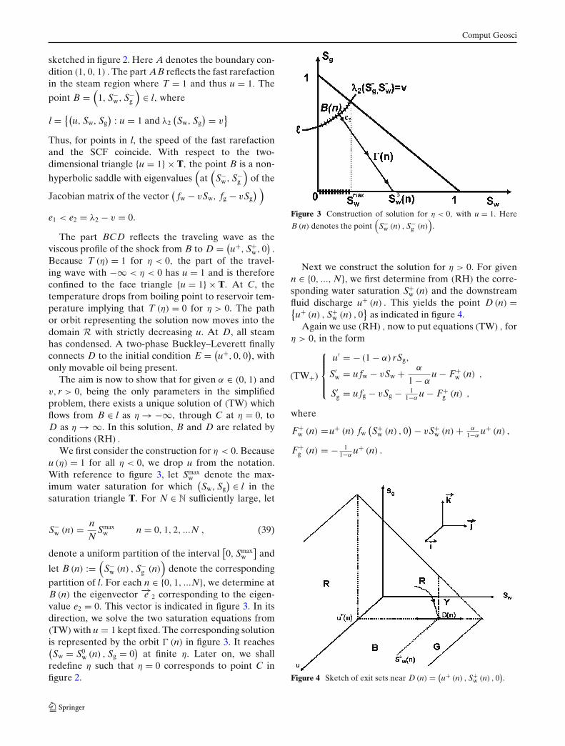
Next we construct the solution for η > 0. For givenn ∈ {0, ..., N}, we first determine from (RH) the corre-sponding water saturation S+

w (n) and the downstreamfluid discharge u+ (n) . This yields the point D (n) ={u+ (n) , S+

w (n) , 0}

as indicated in figure 4.Again we use (RH) , now to put equations (TW) , for

η > 0, in the form

(TW+)

⎧⎪⎪⎨

⎪⎪⎩

u′ = − (1 − α) rSg,

S′w = ufw − vSw + α

1 − αu − F+

w (n) ,

S′g = ufg − vSg − 1

1−αu − F+

g (n) ,

where

F+w (n) =u+ (n) fw

(S+

w (n) , 0) − vS+

w (n) + α1−α

u+ (n) ,

F+g (n) = − 1

1−αu+ (n) .

Figure 4 Sketch of exit sets near D (n) = (u+ (n) , S+

w (n) , 0).

Comput Geosci

We first determine the nature of the stationary pointD (n) . From the Jacobian matrix at D (n), we find onenegative and two positive eigenvalues:

λ1 = −v

2− 1

2

√v2 + 4r < 0

λ2 = −v

2+ 1

2

√v2 + 4r > 0

λ3 = u+ (n)∂ fw

∂Sw

(S+

w (n) , 0) − v > 0

The latter being positive follows directly from aconsistency condition: all characteristic speeds in thetwo-phase Buckley–Leverett regime must exceed thespeed of the SCF (see also [7]). Only the negativeeigenvalue λ1 is relevant, and we have to verify that thecorresponding eigenvector −→e 1 points into domain R.Indeed, a straightforward computation gives

−→e 1 · −→k

−→e 1 · −→i

= 1

2

v + √v2 + 4r

(1 − α) r> 0 for all n ∈ {0, 1, ..., N}.

Here−→i and

−→k are unit vectors as indicated in figure 4.

This inequality shows that −→e 1 points in the direction ofincreasing u and Sg. Part of the orbit representing thesolution (TW+) is sketched in figure 4.

Remark 4.1 An eigenvector corresponding to λ3 is−→e 3 = (0, 1, 0) . Indeed, a solution of (TW+) is (u =u+(n), Sw, Sg = 0) with Sw satisfying

S′w = u+ (

fw (Sw) − fw(S+

w

)) − v (Sw − Sw+) .

Let us now turn to the full solution in R. For a fixedn, with corresponding curve � (n), we solve equations(TW+_

)with points from � (n) as initial condition.

Because u′ < 0, the solution orbit will move into R. Asa first observation, we note that any such orbit cannotleave R through the side

S = {(u, Sw, Sg

) : u+ < u < 1, Sw + Sg = 1}.

Proposition 4.1 Any solution(u (η) , Sw (η) , Sg (η)

)of

(TW+) that belongs to the interior of R for some η =ηo > 0, cannot exit R through S for η > ηo.

Proof We argue by contradiction. Suppose there ex-ists η1 > ηo such that

(u (η) , Sw (η) , Sg (η)

) ∈ int (R) forη < η1 and

(u (η1) , Sw (η1) , Sg (η1)

) ∈ S. Then at η = η1

we must have

ddη

⎛

⎝u

Sw

Sg

⎞

⎠ ·⎛

⎝011

⎞

⎠ = (Sw + Sg

)′ ≥ 0. (40)

However, considering (TW+) at η1 and the fact thatSw + Sg = fw + fg = 1 we find

(Sw + Sg

)′ = −v − u+ f +w + vS+

w + u+

= u+ f +o − vS+

o

= f −o − vS−

o ,

where we used S+g = 0 and the oil mass balance from

(RH) .

We claim that

f −o − vS−

o < 0 for all(

S−w, S−

g

)∈ �, (41)

which would contradict Eq. (40) and complete theproof. Any point B ∈ � is the end point of a fast rar-efaction originating from point A. In terms of the oilsaturation, this rarefaction satisfies, with ξ = x/t,

−ξdSo

dξ+ dfo

dξ= 0 for 0 < ξ < v.

Integrating this expression gives

−vS−o + f −

o +v∫

0

So (ξ) dξ = 0, (42)

which directly implies inequality (41). �

Remark 4.2 Equation (42) expresses the oil balance inthe steam region. In terms of x and t, we havevt∫

0

So (x, t) dx + (f −o − vS−

o

)t = 0 for all t > 0,

where(

f −o − vS−

o

)denotes the oil flux with respect to

the moving front.

Thus, selecting a point on the curve � (n) , the cor-responding solution orbit leaves R through one of thefollowing exit sets (see also figure 4):

R(red) := {Sw = 0} ∪ {u = u+, 0 < Sw < S+

w

}

B(blue) := {Sg = 0, 0 < Sw < S+

w

}

Y(yellow) := {u = u+, S+

w < Sw < 1}

G(green) := {Sg = 0, S+

w < Sw < 1}

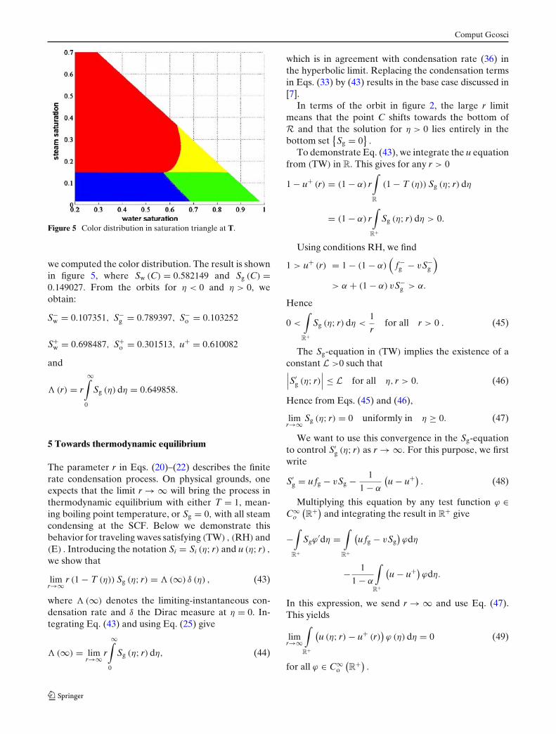
A point on � (n) is now colored red, blue, yellowor green depending on the exit set of the orbit. Forlarge N and for a large number of points on � (n),we cover in this way the front triangle below � withthese four colors. The point where they meet, denotedby C = {

u = 1, Sw (C) , Sg (C)}, and the path through it

determine the unique orbit (traveling wave) through R.For the simplified expressions (37) and (38) and with

v = 0.4, r = 20 and α = 0.4,

Comput Geosci

Figure 5 Color distribution in saturation triangle at T.

we computed the color distribution. The result is shownin figure 5, where Sw (C) = 0.582149 and Sg (C) =0.149027. From the orbits for η < 0 and η > 0, weobtain:

S−w = 0.107351, S−

g = 0.789397, S−o = 0.103252

S+w = 0.698487, S+

o = 0.301513, u+ = 0.610082

and

�(r) = r

∞∫

0

Sg (η) dη = 0.649858.

5 Towards thermodynamic equilibrium

The parameter r in Eqs. (20)–(22) describes the finiterate condensation process. On physical grounds, oneexpects that the limit r → ∞ will bring the process inthermodynamic equilibrium with either T = 1, mean-ing boiling point temperature, or Sg = 0, with all steamcondensing at the SCF. Below we demonstrate thisbehavior for traveling waves satisfying (TW) , (RH) and(E) . Introducing the notation Si = Si (η; r) and u (η; r) ,

we show that

limr→∞ r (1 − T (η)) Sg (η; r) = �(∞) δ (η) , (43)

where �(∞) denotes the limiting-instantaneous con-densation rate and δ the Dirac measure at η = 0. In-tegrating Eq. (43) and using Eq. (25) give

�(∞) = limr→∞ r

∞∫

0

Sg (η; r) dη, (44)

which is in agreement with condensation rate (36) inthe hyperbolic limit. Replacing the condensation termsin Eqs. (33) by (43) results in the base case discussed in[7].

In terms of the orbit in figure 2, the large r limitmeans that the point C shifts towards the bottom ofR and that the solution for η > 0 lies entirely in thebottom set

{Sg = 0

}.

To demonstrate Eq. (43), we integrate the u equationfrom (TW) in R. This gives for any r > 0

1 − u+ (r) = (1 − α) r∫

R

(1 − T (η)) Sg (η; r) dη

= (1 − α) r∫

R+

Sg (η; r) dη > 0.

Using conditions RH, we find

1 > u+ (r) = 1 − (1 − α)(

f −g − vS−

g

)

> α + (1 − α) vS−g > α.

Hence

0 <

∫

R+

Sg (η; r) dη <1

rfor all r > 0 . (45)

The Sg-equation in (TW) implies the existence of aconstant L >0 such that∣∣∣S′

g (η; r)∣∣∣ ≤ L for all η, r > 0. (46)

Hence from Eqs. (45) and (46),

limr→∞ Sg (η; r) = 0 uniformly in η ≥ 0. (47)

We want to use this convergence in the Sg-equationto control S′

g (η; r) as r → ∞. For this purpose, we firstwrite

S′g = ufg − vSg − 1

1 − α

(u − u+)

. (48)

Multiplying this equation by any test function ϕ ∈C∞

o

(R

+)and integrating the result in R

+ give

−∫

R+

Sgϕ′dη =

∫

R+

(ufg − vSg

)ϕdη

− 1

1 − α

∫

R+

(u − u+)

ϕdη.

In this expression, we send r → ∞ and use Eq. (47).This yields

limr→∞

∫

R+

(u (η; r) − u+ (r)

)ϕ (η) dη = 0 (49)

for all ϕ ∈ C∞o

(R

+).

Comput Geosci

Once more, we consider the u-equation, which wemultiply by ψ ∈ C∞

o

(R

+)and integrate in R

+ to find

∫

R+

(u (η; r) − u+ (r)

)ψ ′ (η) dη =

(1 − α) r∫

R+

Sg (η; r) ψ (η) dη.

Because ψ ′ ∈ C∞o

(R

+)as well, we can use Eq. (49) and

obtain

limr→∞ r

∫

R+

Sg (η; r) ψ (η) dη = 0 for all ψ ∈ C∞o

(R

+),

(50)

which implies

limr→∞ rSg (η; r) = 0, pointwisely in η > 0. (51)

To see this, we use the following argument. For eachn ∈ N, n > 1, the interval

(0, 1

n

)must contain a point

ηn where rSg (ηn; r) → 0 as r → ∞. This is a directconsequence of Eq. (50). Hence, for η = ηn and ε > 0,there exists r∗ > 0 such that

rSg (ηn; r) < ε for all r > r∗.

Using this and Eq. (48), we have that Sg (ηn; r) becomessmall with S′

g (ηn; r) < 0, due to the quadratic terms infg for r sufficiently large. Hence

rSg (η; r) < ε for all r > r∗ and η ≥ ηn,

implying statement (51).Thus, we have shown that

limr→∞ r (1 − T (η)) Sg (η; r) = 0, pointwisely in R\ {0}and

�(r) = r∫

R

(1 − T (η)) Sg (η; r) dη = 1 − u+ (r)1 − α

< 1

for all r > 0. This establishes Eq. (43) provided

�(r) = 1 − u+ (r)1 − α

=(

f −g − vS−

g

)(r) (from RH)

(52)

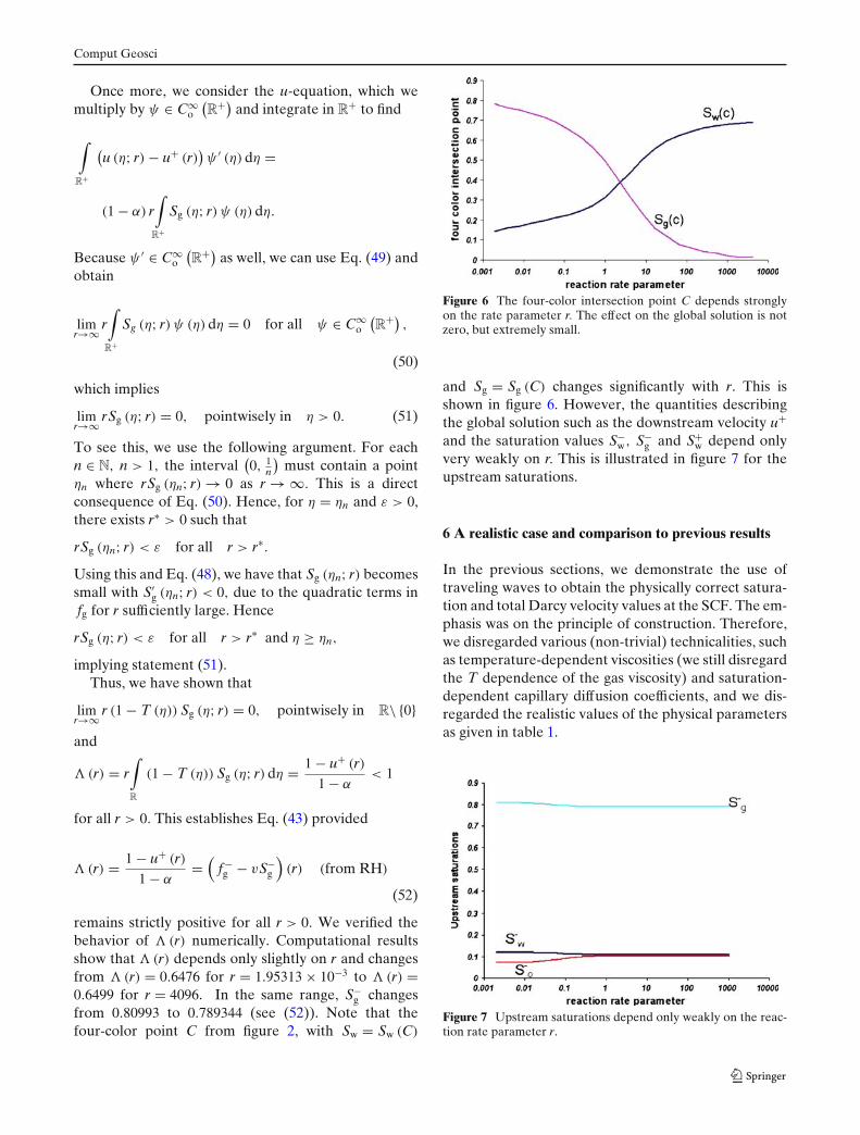
remains strictly positive for all r > 0. We verified thebehavior of �(r) numerically. Computational resultsshow that �(r) depends only slightly on r and changesfrom �(r) = 0.6476 for r = 1.95313 × 10−3 to �(r) =0.6499 for r = 4096. In the same range, S−

g changesfrom 0.80993 to 0.789344 (see (52)). Note that thefour-color point C from figure 2, with Sw = Sw (C)

Figure 6 The four-color intersection point C depends stronglyon the rate parameter r. The effect on the global solution is notzero, but extremely small.

and Sg = Sg (C) changes significantly with r. This isshown in figure 6. However, the quantities describingthe global solution such as the downstream velocity u+and the saturation values S−

w, S−g and S+

w depend onlyvery weakly on r. This is illustrated in figure 7 for theupstream saturations.

6 A realistic case and comparison to previous results

In the previous sections, we demonstrate the use oftraveling waves to obtain the physically correct satura-tion and total Darcy velocity values at the SCF. The em-phasis was on the principle of construction. Therefore,we disregarded various (non-trivial) technicalities, suchas temperature-dependent viscosities (we still disregardthe T dependence of the gas viscosity) and saturation-dependent capillary diffusion coefficients, and we dis-regarded the realistic values of the physical parametersas given in table 1.

Figure 7 Upstream saturations depend only weakly on the reac-tion rate parameter r.

Comput Geosci

In this section, we are going to carry out the construc-tion in a more realistic setting with the aim to explicitthe influence of the finite condensation rate under morepractical circumstances. We also give a comparison tothe results in [7], where we considered several exten-sions, but all under equilibrium conditions.

With reference to table 1, we introduce

• Temperature-dependent viscosities, yielding thetemperature-dependent viscosity ratios

Mow = μo

μwand Mgw = μg

μw.

• Brooks–Corey capillary pressures (see [1]), yieldingadditional terms in the expressions for water andgas discharge [see Eqs. (14)–(17)].

• Different relative permeabilities. As in [7], we con-sider fourth-order power-law expressions as well asunnormalized Stone I formulas (see [9, 17]):

krw = krw (Swe) = 1

2S

2+3λsλs

we (53)

krg = krg(Sge

) = (1 − Sge)2(1 − S

2+λsλs

ge ) (54)

kro = kSo(1 − Swc)krg (Swe) krw(Sge

)

(1 − Sw)(1 − Swc − Sg)(55)

where Swe = Sw−Swc1−Swc

, Sge = 1−Sg−Swc

1−Swc. Using a gas

saturation-dependent residual oil saturation is forthe steam drive problem an unnecessary complica-tion, and therefore, we assume that the residual oilsaturation is always zero.

With these extensions, the model equations in fulldimensional form are

∂u∂x

= − (1 − α)qρg

, (56)

ϕ∂Sw

∂t+ ∂

∂x

(

ufw − Dww∂Sw

∂x− Dwg

∂Sg

∂x

)

= qρw

, (57)

ϕ∂Sg

∂t+ ∂

∂x

(

ufg − Dgw∂Sw

∂x− Dgg

∂Sg

∂x

)

= − qρg

. (58)

Note that the fractional flow functions fα, and hencethe diffusivities Dαβ, are discontinuous across the SCF.This is due to the temperature dependence of the mo-bility ratios.

Using Eq. (56) to estimate q from Eqs. (57) and (58),substituting Eq. (1) in Eq. (56) and applying the scalings(18) and (19) gives

∂u∂x

= −qbLuinj

(1 − α) (1 − T)Sg, (59)

∂Sw

∂t+ ∂

∂x

(

ufw−D∗(

Jww∂Sw

∂x+Jwg

∂Sg

∂x

))

= α

α − 1

∂u∂x

,

(60)

∂Sw

∂t+ ∂

∂x

(

ufg−D∗ ∂

∂x

(

Jgw∂Sw

∂x+Jgg

∂Sg

∂x

))

=− 1

α−1

∂u∂x

,

(61)

Here

D∗ = σ

μ∗wLuinj

√kϕ

(12 − Swc

1 − Swc

)1/λs

where again μ∗w is an appropriately chosen character-

istic water viscosity (here the viscosity at the initialreservoir temperature) and

Jww = μ∗w

μw

λs fw

1 − Swc

(kro

Mow+ krg

Mgw

)(Sw − Swc

1 − Swc

)−1/λs−1

,

Jwg = −μ∗w

μw

λs fw

1 − Swc

krg

Mgw

(1 − Sg − Swc

1 − Swc

)−1/λs−1

,

Jgw = −μ∗w

μw

λs fg

1 − Swckrw

(Sw − Swc

1 − Swc

)−1/λs−1

,

Jgg = μ∗w

μw

λs fg

1 − Swc

(kro

Mow+krw

)(1 − Sg − Swc

1 − Swc

)−1/λs−1

.

(62)

Introducing the reciprocal Peclet number ε and thedimensionless rate constant r as

ε := σ

μ∗wLuinj

√Kϕ

(12 − Swc

1 − Swc

)1/λs

, (63)

r := qbσ

μ∗wu2

inj

√Kϕ

(12 − Swc

1 − Swc

)1/λs

= εqbL

uinj, (64)

applying a traveling wave coordinate transformationη = (x − vt) /ε and integrating the resulting equationsleads to the system, with −∞ < η < ∞,

u′ = −r (1 − α) (1 − T)Sg, (65)

JwwS′w+JwgS′

g = ufw−vSw−α (1−u)

1−α− (ufw − vSw)

−

(66)

JgwS′w+JggS′

g = ufg−vSg− u−1

1−α− (

ufg−vSg)−

, .

(67)

Note that qbL/uinj, the Damkohler number, is con-sidered to be of the same order of magnitude as thePeclet number 1/ε. As before, we look for solutions

Comput Geosci

satisfying boundary conditions (BC) subject to the con-straints (E) and (RH). Note that Eqs. (65)–(67) reduceto (TW) when Jwg = Jgw = 0 and Jww = Jgg = 1.

Equations (65) and (67) can be rearranged to explicitexpressions for S′

w and S′g if the determinant

∣∣∣∣Jww Jwg

Jgw Jgg

∣∣∣∣ = 0.

It is straightforward to verify these conditions. Detailsare omitted. The rearranged equations, with explicit S′

w

and S′g are used in the numerical procedure.

6.1 Procedure for determining the traveling wave orbit

The procedure to find the traveling wave describing theprocesses in the SCF for the realistic case is slightlydifferent from the procedure used in the previoussections. The reason is that we need a more robustmethod for solutions with small values of the reactionrate parameter r, for which the four color point (seefigure 5) approaches the line � satisfying condition (30).Our aim is to find the orbit D − −C − −B (n) satis-fying Eqs. (65)–(67), satisfying the Rankine–Hugoniotconditions and condition (30). First we choose as aninitial guess a value n′ and determine as in (39) thecorresponding value of Sw

(n′). Subsequently, we ap-

ply condition (30) to determine Sg(n′) and thus point

B(n′) on � (see figure 8). Subsequently, we determine

from the left (upstream) values of(

u− = 1, S−w, S−

g

)

at B(n′) the right (downstream) values

(u+, S+

w, S+g

),

i.e. point D′ in figure 8, using the Rankine–Hugoniotconditions (29). At the equilibrium point B

(n′), we

Figure 8 The orbits from(

u− = 1, S−g , S−

w

)in the plane u = 1

and orbits in the negative η direction from(

u+, S+g , S+

w

)that

intersect in the u = 1 plane at C are found using bissection(see text).

determine the eigenvector to obtain the first point onthe orbit away from it. We use this point as initialcondition for the rearranged conditions (65)–(67) in thehot-upstream-region, and we determine as before thecorresponding orbit until we hit Sg = 0. We computethe orbit emanating from B

(n′) using Eq. (65)–(67) in

the positive η direction until we hit the Sg = 0 axis. Wecall this orbit �

(n′) . At the downstream point D′ =

(u+, S+

w, S+g

), we apply a similar procedure; that is, we

determine the eigenvector pointing into the domain Rto obtain the first point away from this equilibriumpoint. Then we solve the rearranged Eqs. (65)–(67) inthe cold-downstream region, this time in the negativeη direction until we hit the u = 1 plane with values(Sw

(C′) , Sg

(C′)) (see figure 8). We choose a second

guess, e.g. n′, to start at a new point B(n′) to the right or

left with respect to B(n′) depending on whether Sw

(C′)

was to the right or to the left of �(n′) and repeat the

procedure above. For the sequence of points n′, n′, ...,we use a bisection routine until we approximate thecomplete orbit B (n) − C − D, with

(Sw (C ) , Sg (C )

)on

the orbit � (n).

6.2 Results

Figure 9 shows the upstream oil saturation as a functionof the reaction rate parameter. We distinguish fourcases where we use either Stone I expressions (53-55)(ST) or power-law expressions (PL) for the relativepermeability and either a constant capillary diffusion(D) (see table 1) or a saturation-dependent capillarydiffusion coefficient (Pc) (see (17)). Figure 9 also shows,for each of these cases, the oil saturation obtained when

Figure 9 Upstream oil saturation as a function of the reactionrate parameter. There are four cases. PL = power-law relativepermeabilities, ST = Stone I relative permeabilities, D = con-stant capillary diffusion, Pc =saturation-dependent capillarydiffusion. The points (Eq, PL, D), (Eq, PL, Pc), (Eq, ST, D)and (Eq, PL, Pc) correspond to the solutions obtained for ther-modynamic equilibrium.

Comput Geosci

thermodynamic equilibrium is assumed [7]. As to beexpected from Section 5, the oil saturation values areabout equal to the values obtained for large reactionrate parameters. It is evident that in all cases, the globalsolution depends strongly on the capillary pressure be-havior for the same relative permeability expressions.The numerical results, shown in figure 9, suggest thatthe global solution in terms of the values S−

w, S−g , S+

w, u+is very insensitive to the reaction rate parameter exceptfor the case where we combine saturation-dependentcapillary pressures and Stone I expressions for the rela-tive permeabilities.

7 Conclusions

1. A hyperbolic model for steam displacement of oilwas extended with a finite rate condensation modelin the transition zone.

2. The traveling wave describing the shock solutionis a saddle-to-saddle connection. Consequently, theglobal solution depends on the details of the con-densation model within the shock.

3. Using color coding, it has been shown numeri-cally that, given the parameters describing the con-densation process, there is a unique set of valuesS−

w, S−g , S+

w, u+, etc., for which a traveling waveexists (see figure 5).

4. A proof was given that the solution with an in-finite reaction rate parameter tends to the solu-tion obtained when thermodynamic equilibrium isassumed.

5. The numerical solutions show that there is a depen-dence of the global solution on the reaction rateparameter. For power-law relative permeabilities,this dependence is very weak.

6. The procedure described can also be used for arealistic set of input variables. When we com-bine Stone I relative permeabilities with saturation-dependent capillary pressures, the effect of thereaction rate parameter is significant.

Acknowledgement We acknowledge D. Marchesin [Institutode Matemática Pura é Aplicada, Rio de Janeiro (Brazil)] for hissuggestion of color coding the orbits in the triangle T. This workwas partially carried out at the Institute for Mathematics and itsApplication (IMA), Minneapolis, MN.

References

1. Aziz, K., Settari, A.: Petroleum Reservoir Simulation. Ap-plied Science Publishers, London (1979)

2. Bear, J.: Dynamics of Fluids in Porous Media. Dover Publi-cations, Inc., Dover (1972)

3. Betz, C., Farbar, A., Schmidt, R.: Removing Volatile andSemi-Volatile Contaminants from the Unsaturated Zone byInjection of a Steam Air Mixture. Thomas Telford. Contami-nated Soil (1998)

4. Bird, R., Stewart, W., Lightfoot, E.: Transport Phenomena.John-Wiley, New York (1960)

5. Brantferger, R., Pope, G., Sepehrnori, K.: Development of athermodynamically consistent, fullyImplicit equation of state,ompositional steamfllod simulator. SPE 21253. SPE Sympo-sium Reservoir Simulation, Anaheim (1991)

6. Brooks, R., Corey, A.: Properties of porous media affectingfluid. Flow. J. Irrig. Drain. Div. 6, 61 (1966)

7. Bruining, J., van Duijn, C.: Uniqueness conditions in a hyper-bolic model for oil recovery by steamdrive. Comput. Geosci.4, 65–98 (2000)

8. Chien, M., Yardumian, H., Chung, E., Todd, W.: Theformulation of a thermal simulation model in a vec-torized, general purpose reservoir simulator. SPE 18418.The SPE Symposium on Reservoir Simulation in Houston(1989)

9. Fayers, F.J., Matthews, J.: Evaluation of normalized Stone’smethods for estimating three-phase relative permeabilities.Soc. Pet. Eng. J. 224–232 (1984)

10. Fayers, F.J., Sheldon, J.: The effect of capillary pressure andgravity on two-phase fluid flow in a porous medium. Trans.AIME 216, 147 (1959)

11. Goderij, R., Bruining, J., Molenaar, J.: A fast 3D inter-face simulator for steam drives. SPE J. 4 (4), 400–408.SPE-Western Regional Meeting (June-1997) 279-289 (SPE-38288)(1999)

12. Grabensetter, J., Li, Y.-K., Collins, D., Nghiem, L.: Stabilitybased switching criterion for adaptive-implicit compositionalreservoir simulation. SPE Symposium Reservoir SimulationAnaheim (1991) SPE 21225 (1991)

13. Gümrah, F., Palmgren, C., Bruining, J., Godderij, R.: Steam-drive in a layered reservoir: an experimental and theoreticalstudy. In: Proc. SPE/DOE 8th Symposium on Enhanced OilRecovery, Tulsa SPE/DOE 24171, 159–167 (1992)

14. Guzman, R., Fayers, F.: Mathematical properties of three-phase flow equations. SPE J. 2, 291–300 (1997a)

15. Guzman, R., Fayers, F.: Solutions to the three-phaseBuckley–Leverett problem. SPE J. 2, 301–311 (1997b)

16. Hanzlik, E., Mims, D.: Forty years of steam injection inCalifornia—evolution of heat management. SPE Interna-tional Improved Oil Recovery Conference in Asia KualaLumpur Malaysia, SPE 84848 (2003)

17. Honarpour, M., Koederitz, L., Harvey, A.: Relative Perme-ability of Petroleum Reservoirs. Boca Raton, Florida, USA:CRC Press (1986)

18. Hovanessian, S., Fayers, F.: Linear waterflood with gravityand capillary effects. Soc. Pet. Eng. J. I, 32 (1961)

19. Hunt, J., Sitar, N., Udell, K.: Non-aqueous phase liquid trans-port and clean up: part I, analysis of mechanisms. WaterResour. Res. 24 (8), 1247–1258 (1988a)

20. Hunt, J., Sitar, N., Udell, K.: Non-aqueous phase liquid trans-port and clean up: part II, experimental studies. Water Re-sour. Res. 24 (8), 1259–1269 (1988b)

21. Isaacson, E., Marchesin, D., Plohr, B.: Transitional waves forconservation laws. SIAM J. Math. Anal. 21, 837–866 (1990)

22. Isaacson, E., Marchesin, D., Plohr, B., Temple, J.: Multi-phase flow models with singular Riemann problems. Math.Appl. Comput. 2, 147–166 (1992)

23. Kaslusky, S., Udell, K.: A theoretical model of air andsteam co-injection to prevent the downward migration of

Comput Geosci

the DNAPL’s during steam enhanced extraction. J. Contam.Hydrol. 55, 213–232 (2002)

24. Kimber, K., Ali, S.F., Puttagunta, V.: New scaling criteria andtheir relative merits for steam recovery experiments. J. Can.Petrol. Technol. 27, 86–94 (1988)

25. Lax, P.: The formation and decay of shock waves. Am. Math.Monthly 79, 227–241 (1988)

26. Mandl, G., Volek, C.: Heat and mass transport in steamdriveprocesses. Soc. Pet. Eng. J. 57–79 (1969)

27. Marchesin, D., Schaeffer, D., Shearer, M., Paes-Leme: Theclassification of 2 × 2 systems of non-strictly hyperbolic con-servation laws, with application to oil recovery. Comm. PureAppl. Math. 40, 141–178 (1987)

28. Menegus, D., Udell, K.: A study of steam injection into watersaturated porous media, heat transfer in porous media andparticle flows. ASME Heat Transf. Div. New York City. 46,151–157 (1985)

29. Mifflin, R., Watts, J.: A fully coupled, fully implicit simula-tor for thermal and other complex reservoir processes. SPE21252 Symposium Reservoir Simulation, Anaheim (1991)21252 (1969)

30. Naccache, P.: A fully implicit thermal reservoir simulator.SPE 37985 Reservoir Simulatiuon Symposium, Dallas (1997)

31. Oballa, V., Coombe, D., Buchanan, W.: Adaptive-implicitmethod in thermal simulation. SPE Reserv. Eng. 549–556(1990)

32. Prats, M.: Thermal Recovery. Dallas: SPE Henry L. DohertySeries, Monograph 7 (1982)

33. Rapoport, L.: Scaling laws for use in design and operation ofwater–oil flow models. Trans. AIME 204, 143 (1955)

34. Rapoport, L., Leas, W.: Properties of linear waterfloods.Trans. AIME 198, 139–148 (1953)

35. Reid, R., Parausnitz, J., Sherwood, T.: The Properties ofGases and Liquids. New York: McGraw-Hill (1977)

36. Rose, W., Bruce, W.: Evaluation of capillary charactersin petroleum reservoir rock. Trans. AIME 186, 127–142(1949)

37. Schmidt, R., Betz, C., Faerber, A.: LNAPL and DNAPL be-haviour during steam injection into the unsaturated zone. Int.Assoc. Hydrol. Sci. Publ. 250, 11–117 (1998)

38. Schmidt, R., Gudbjerg, J., Sonnenborg, T.O., Jensen, K.: Re-moval of NAPL’s from the unsaturated zone using steam:prevention of downsward migration by injecting mixtures ofsteam and air. J. Contam. Hydrol. 55, 233–260 (2002)

39. Shutler, N.: A one dimensional analytical technique for pre-dicting oil recovery by steam flooding. Soc. Pet. Eng. J. 489–498 (1972)

40. Stewart, L., Udell, K.: Mechanisms of residual oil displace-ment by steam injection. SPE Reserv. Eng. 1233–1242 (1988)

41. Tortike, W., Farouq-Ali, S.: Saturated-steam-property func-tional correlations for fully implicit thermal reservoir simula-tion. SPE Reserv. Eng. 4(4), 471–474 (1989)

42. Udell, K.: The thermodynamics of evaporation and con-densation in porous media. SPE 10779, California Re-gional Meeting of the Society of Petroleum Engineers, SanFrancisco (1982)

43. Willman, B., Valeroy, V., Runberg, G., Cornelius, A.: Lab-oratory studies of oil recovery by steam injection. J. Petrol.Technol. 681–690 (1961)

44. Wingard, J., Orr, F.: An analytical solution for steam/oil/water displacements. SPE Adv. Technol. Ser. 2, 167–176(1994)

45. Yortsos, Y.: Distribution of fluid phases within the steamzone in steam injection processes. Soc. Pet. Eng. J. 458–466(1984)

46. Yortsos, Y., Gavalas, G.: Heat transfer ahead of movingcondensation fronts in thermal oil recovery processes. Int. J.Heat Mass Transfer 25(3), 305–316 (1982)