Traveling surface waves of moderate amplitude

in shallow water

Armengol Gasull and Anna Geyer∗

Departament de Matematiques, Facultat de Ciencies,Universitat Autonoma de Barcelona, 08193 Bellaterra, Barcelona, Spain.

December 20, 2013

Abstract

We study traveling wave solutions of an equation for surface waves of moderate amplitudearising as a shallow water approximation of the Euler equations for inviscid, incompressibleand homogenous fluids. We obtain solitary waves of elevation and depression, including afamily of solitary waves with compact support, where the amplitude may increase or decreasewith respect to the wave speed. Our approach is based on techniques from dynamical systemsand relies on a reformulation of the evolution equation as an autonomous Hamiltonian systemwhich facilitates an explicit expression for bounded orbits in the phase plane to establishexistence of the corresponding periodic and solitary traveling wave solutions.

1 Introduction and main result

A number of competing nonlinear model equations for water waves have been proposed to thisday to account for fascinating phenomena, such as wave breaking or solitary waves, which arenot captured by linear theory. The well-known Camassa–Holm equation [4] is one of the mostprominent examples, due to its rich structural properties. It is an integrable infinite-dimensionalHamiltonian system [1, 6, 10] whose solitary waves are solitons [12, 18]. Some of its classicalsolutions develop singularities in finite time in the form of wave breaking [8], and recover inthe sense of global weak solutions after blow up [2, 3]. For a classification of its weak travelingwave solutions we refer to [25]. The manifold of its enticing features led Johnson to demonstratethe relevance of the Camassa–Holm equation as a model for the propagation of shallow waterwaves of moderate amplitude. He proved that the horizontal component of the fluid velocityfield at a certain depth within the fluid is indeed described by a Camassa–Holm equation [7, 23].Constantin and Lannes [11] followed up on the matter in search of a suitable correspondingequation for the free surface and derived an evolution equation for surface waves of moderateamplitude in the shallow water regime,

ut + ux + 6uux − 6u2ux + 12u3ux + uxxx − uxxt + 14uuxxx + 28uxuxx = 0, (1)

The authors show that equation (1) approximates the governing equations to the same orderas the Camassa–Holm equation, and also prove that the Cauchy problem on the line associated

∗Corresponding author. E-mail: annageyer@mat.uab.cat

1

This is a preprint of: “Traveling surface waves of moderate amplitude in shallow water”, ArmengolGasull, Anna Geyer, Nonlinear Anal., num. 102, 105–119, 2014.DOI: [10.1016/j.na.2014.02.005]

to (1), is locally well-posed [11]. Employing a semigroup approach due to Kato [24], Duruk[15] shows that this results also holds true for a larger class of initial data, as well as for thecorresponding spatially periodic Cauchy problem [14]. Consequently, solutions of (1) dependcontinuously on their initial data in Hs for s > 3/2, and it can be shown that this dependenceis not uniformly continuous [17]. In the context of Besov spaces, well-posedness is discussed[27] using Littlewood-Paley decomposition, along with a study about analytic solutions andpersistence properties of strong solutions. One of the important aspects of equation (1) lies in itsrelevance for capturing the non-linear phenomenon of wave breaking [11, 15], a feature it shareswith the Camassa-Holm equation. While the latter equation is known to possess global solutions[3, 9], it is not apparent how to obtain global control of the solutions of equation (1), owing toits involved structure and due to the higher order nonlinearities. However, passing to a movingframe one can study so-called traveling wave solutions, whose wave profiles move at constantspeed in one direction without altering their shape. Introducing the traveling wave Ansatz

ξ = x− c t, u(ξ) = u(t, x), (2)

equation (1) reads

d

dξ

((1− c)u+ 3u2 − 2u3 + 3u4 + (1 + c+ 14u) u+ 7 u

)= 0 (3)

where the dot denotes differentiation with respect to ξ. Existence of smooth solitary wavesolutions of (3) which decay to zero at infinity has been established [20] for wave speeds c > 1,and their orbital stability has been deduced [16] employing an approach due to Grillakis, Shatahand Strauss [21] taking advantage of the Hamiltonian structure of (1). In the present paper weset out to improve the existence result [20] by loosening the assumption that solitary waves tendto zero at infinity. Allowing for a decay to an arbitrary constant, we establish existence of avariety of novel traveling wave solutions of (1).

Theorem 1.1. For every speed c ∈ R\c∗ there exist peaked periodic, as well as smooth solitaryand periodic traveling wave solutions of (1). Periodic waves may be obtained also for c = c∗,where c∗ ≈ 0.35328 is the unique real solution of 3 c3 + 30 c2 + 1031 c− 368 = 0.

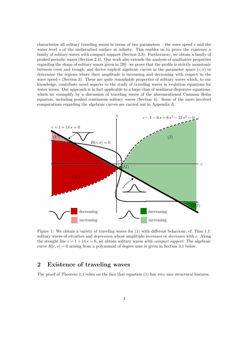
Moreover, the solitary waves can be characterized in terms of two parameters – the wave speed cand the level of the undisturbed water surface s – allowing us to determine the exact regions inthis parameter space which give rise to the following types of waves, cf. Figure 1:

• Solitary waves in C1 with compact support on R (along the straight line c+ 1 + 14 s = 0).

• Smooth solitary waves of elevation whose amplitude is strictly increasing (in region I) ordecreasing (in regions II and III) with respect to c.

• Smooth solitary waves of depression whose amplitude is strictly increasing (in region V)or decreasing (in region IV) with respect to c.

All solitary waves are symmetric with respect to their unique crest/trough, they are monotonicand decay exponentially to the undisturbed water surface s at infinity.

The proof of these results hinges on the observation that for traveling waves, equation (1) maybe written as an autonomous Hamiltonian system involving two parameters. This insight allowsus to explicitly determine bounded orbits in the phase plane which correspond to solitary andperiodic traveling waves of elevation as well as depression (Section 2.1 and 2.2). Moreover, we

2

characterize all solitary traveling waves in terms of two parameters – the wave speed c and thewater level s of the undisturbed surface at infinity. This enables us to prove the existence afamily of solitary waves with compact support (Section 2.3). Furthermore, we obtain a family ofpeaked periodic waves (Section 2.4). Our work also extends the analysis of qualitative propertiesregarding the shape of solitary waves given in [20]: we prove that the profile is strictly monotonicbetween crest and trough, and derive explicit algebraic curves in the parameter space (c, s) todetermine the regions where their amplitude is increasing and decreasing with respect to thewave speed c (Section 3). These are quite remarkable properties of solitary waves which, to ourknowledge, contribute novel aspects to the study of traveling waves in evolution equations forwater waves. Our approach is in fact applicable to a large class of nonlinear dispersive equations,which we exemplify by a discussion of traveling waves of the aforementioned Camassa–Holmequation, including peaked continuous solitary waves (Section 4). Some of the more involvedcomputations regarding the algebraic curves are carried out in Appendix A.

(I)

(III)

(II)

c∗

(IV )

(V )

c

s

c+ 1 + 14 s = 0

c− 1− 6 s+ 6 s2 − 12 s3 = 0

R(c, s) = 0

decreasing

increasing

decreasing

increasing

Figure 1: We obtain a variety of traveling waves for (1) with different behaviour, cf. Thm 1.1:solitary waves of elevation and depression whose amplitude increases or decreases with c. Alongthe straight line c+ 1 + 14 s = 0, we obtain solitary waves with compact support. The algebraiccurve R(c, s) = 0 arising from a polynomial of degree nine is given in Section 3.1 below.

2 Existence of traveling waves

The proof of Theorem 1.1 relies on the fact that equation (1) has very nice structural features.

3

2.1 Hamiltonian Formulation

Consider a general partial differential equation which, upon introducing the traveling wave Ansatz(2) can be transformed into an autonomous ordinary differential equation of the form

u (u− u) +1

2(u)2 + F ′(u) = 0, (4)

where u is a constant, F (u) is a smooth function and the dot denotes differentiation with respectto ξ. The corresponding planar system is given by

u = v

v =−F ′(u)− 1

2 v2

u− u ,(5)

and we observe that a reparametrisation of the independent variable according to dξdτ = u − u

transforms (5) into

u′ = (u− u) v

v′ = −F ′(u)− 12 v

2,(6)

where the prime denotes differentiation with respect to τ . The latter system is clearly topo-logically equivalent to the former (cf. [13, 22]) on each connected component of R\u = u,preserving orientation in the open half-plane u > u and reversing orientation in the other half.The advantage of (6) is that it possesses a Hamiltonian

H(u, v) = F (u) +1

2v2 (u− u) = h (7)

satisfying u′ = Hv and v′ = −Hu, which is constant along the solution curves of (6). Explicitknowledge of the critical points and (closed) orbits

v = ±√

2h− F (u)

u− u (8)

in the phase plane of (6) therefore completely characterizes the smooth traveling wave solutionsof the partial differential equation. Applying these ideas to (1) and integrating the associatedequation for traveling waves (3) yields

(1− c)u+ 3u2 − 2u3 + 3u4 + (1 + c+ 14u) u+ 7 u = −14K,

for some constant K ∈ R, which may be written in the form (4) with

F (u) = K u+1− c

28u2 +

1

14u3 − 1

28u4 +

3

70u5, (9)

and

u = −1 + c

14.

In view of the above considerations, we obtain the following existence result for bounded travelingwave solutions of (1):

4

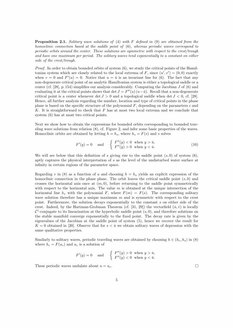
Proposition 2.1. Solitary wave solutions of (4) with F defined in (9) are obtained from thehomoclinic connection based at the saddle point of (6), whereas periodic waves correspond toperiodic orbits around the center. These solutions are symmetric with respect to the crest/troughand have one maximum per period. The solitary waves tend exponentially to a constant on eitherside of the crest/trough.

Proof. In order to obtain bounded orbits of system (6), we study the critical points of the Hamil-tonian system which are closely related to the local extrema of F , since (u′, v′) = (0, 0) exactlywhen v = 0 and F ′(u) = 0. Notice that u = u is an invariant line for (6). The fact that anynon-degenerate critical point of an analytic Hamiltonian system is either a topological saddle or acenter (cf. [28], p. 154) simplifies our analysis considerably. Computing the Jacobian J of (6) andevaluating it at the critical points shows that det J = F ′′(u) (u−u). Recall that a non-degeneratecritical point is a center whenever det J > 0 and a topological saddle when det J < 0, cf. [28].Hence, all further analysis regarding the number, location and type of critical points in the phaseplane is based on the specific structure of the polynomial F , depending on the parameters c andK. It is straightforward to check that F has at most two local extrema and we conclude thatsystem (6) has at most two critical points.

Next we show how to obtain the expressions for bounded orbits corresponding to bounded trav-eling wave solutions from relation (8), cf. Figure 2, and infer some basic properties of the waves.Homoclinic orbits are obtained by letting h = hs, where hs = F (s) and s solves

F ′(y) = 0 and

F ′′(y) < 0 when y > u,F ′′(y) > 0 when y < u.

(10)

We will see below that this definition of s giving rise to the saddle point (s, 0) of system (6),aptly captures the physical interpretation of s as the level of the undisturbed water surface atinfinity in certain regions of the parameter space.

Regarding v in (8) as a function of u and choosing h = hs yields an explicit expression of thehomoclinic connection in the phase plane. The orbit leaves the critical saddle point (s, 0) andcrosses the horizontal axis once at (m, 0), before returning to the saddle point symmetricallywith respect to the horizontal axis. The value m is obtained at the unique intersection of thehorizontal line hs with the polynomial F , where F (m) = F (s). The corresponding solitarywave solution therefore has a unique maximum m and is symmetric with respect to the crestpoint. Furthermore, the solution decays exponentially to the constant s on either side of thecrest. Indeed, by the Hartman-Grobman Theorem (cf. [31, 29]) the vectorfield (u, v) is locallyC1-conjugate to its linearization at the hyperbolic saddle point (s, 0), and therefore solutions onthe stable manifold converge exponentially to the fixed point. The decay rate is given by theeigenvalues of the Jacobian at the saddle point of system (5), hence we recover the result forK = 0 obtained in [20]. Observe that for s < u we obtain solitary waves of depression with thesame qualitative properties.

Similarly to solitary waves, periodic traveling waves are obtained by choosing h ∈ (hc, hs) in (8)where hc = F (uc) and uc is a solution of

F ′(y) = 0 and

F ′′(y) > 0 when y > u,F ′′(y) < 0 when y < u.

These periodic waves undulate about u = uc.

5

F (u)

hs

hp

u

v

u mucs

hsm

s

hp

s

ξ

ξ

Figure 2: A sketch of how bounded orbits in the (u, v) phase plane are obtained using relation (8),where choosing h = hp and h = hs give rise to periodic and solitary traveling waves, respectively.

2.2 Conditions for the existence of solitary traveling waves

We now derive algebraic conditions for the existence of homoclinic orbits, which give rise tosolitary traveling wave solutions of (1) as we have just seen. At this point, our problem involvesthree interdependent parameters:

c . . . the wave speed,K . . . the constant of integration,s . . . the level of the undisturbed water surface at infinity.

It turns out to be more convenient to eliminate the parameter K in favor of s using relationF ′(s) = 0 from the definition (10) of s. This leads us to the following change of parameters:

Φ : (c, s) 7−→ (c,K) = (c, ϕ(c, s)), (11)

where

ϕ(c, s) =1

14s (−3 s3 + 2 s2 − 3 s+ c− 1). (12)

Remark 2.2. Notice that Φ is not bijective on R2 . For instance, for each c ∈ R and K bigenough the point (c,K) has no preimage. However, this happens precisely when there areno simple solutions of F ′(s) = 0, in which case system (6) does not have homoclinic orbits.In the remaining cases, observe that for each fixed c ∈ R there exist two s1 6= s2 such thatϕ(c, s1) = ϕ(c, s2) = (c,K). This leads to a redundancy in the parameter regions, since for eachc there are two values s which yield the same K, and hence the same F , which gives rise to thesame phase portrait of system (6), and therefore also to the same wave solution. The differencebetween the two values of s is that one of them, say s1, satisfies (10) and hence corresponds tothe saddle point of system (6), thus reconciling the interpretation of s being the undisturbed

6

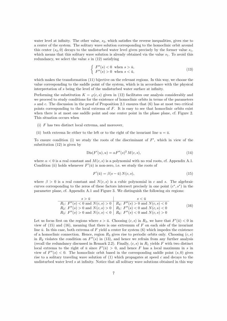
water level at infinity. The other value, s2, which satisfies the reverse inequalities, gives rise toa center of the system. The solitary wave solution corresponding to the homoclinic orbit aroundthis center (s2, 0) decays to the undisturbed water level given precisely by the former value s1,which means that this solitary wave solution is already obtained via the value s1. To avoid thisredundancy, we select the value s in (12) satisfying

F ′′(s) < 0 when s > u,F ′′(s) > 0 when s < u,

(13)

which makes the transformation (11) bijective on the relevant regions. In this way, we choose thevalue corresponding to the saddle point of the system, which is in accordance with the physicalinterpretation of s being the level of the undisturbed water surface at infinity.

Performing the substitution K = ϕ(c, s) given in (12) facilitates our analysis considerably andwe proceed to study conditions for the existence of homoclinic orbits in terms of the parameterss and c. The discussion in the proof of Proposition 2.1 ensures that (6) has at most two criticalpoints corresponding to the local extrema of F . It is easy to see that homoclinic orbits existwhen there is at most one saddle point and one center point in the phase plane, cf. Figure 2.This situation occurs when

(i) F has two distinct local extrema, and moreover,

(ii) both extrema lie either to the left or to the right of the invariant line u = u.

To ensure condition (i) we study the roots of the discriminant of F ′, which in view of thesubstitution (12) is given by

Dis(F ′(u), u) = αF ′′(s)2M(c, s), (14)

where α < 0 is a real constant and M(c, s) is a polynomial with no real roots, cf. Appendix A.1.Condition (ii) holds whenever F ′(u) is non-zero, i.e. we study the roots of

F ′(u) = β(s− u)N(c, s), (15)

where β > 0 is a real constant and N(c, s) is a cubic polynomial in c and s. The algebraiccurves corresponding to the zeros of these factors intersect precisely in one point (c∗, s∗) in theparameter plane, cf. Appendix A.1 and Figure 3. We distinguish the following six regions:

s > u s < uR1: F ′′(s) < 0 and N(c, s) > 0 R4: F ′′(s) > 0 and N(c, s) < 0R2: F ′′(s) > 0 and N(c, s) > 0 R5: F ′′(s) < 0 and N(c, s) < 0R3: F ′′(s) > 0 and N(c, s) < 0 R6: F ′′(s) < 0 and N(c, s) > 0

(16)

Let us focus first on the regions where s > u. Choosing (c, s) in R3, we have that F ′(u) < 0 inview of (15) and (16), meaning that there is one extremum of F on each side of the invariantline u. In this case, both extrema of F yield a center for system (6) which impedes the existenceof a homoclinic connection. Hence, region R3 gives rise to periodic orbits only. Choosing (c, s)in R2 violates the condition on F ′′(s) in (13), and hence we refrain from any further analysis(recall the redundancy discussed in Remark 2.2). Finally, (c, s) in R1 yields F with two distinctlocal extrema to the right of u since F ′(u) > 0, and hence F has a local maximum in s inview of F ′′(s) < 0. The homoclinic orbit based in the corresponding saddle point (s, 0) givesrise to a solitary traveling wave solution of (1) which propagates at speed c and decays to theundisturbed water level s at infinity. Notice that all solitary wave solutions obtained in this way

7

R1

R2R3

R4

R5 R6

(c∗, s∗)

s

c

A1 : F ′′(s) = 0

A2 : s = u

N(c, s) = 0

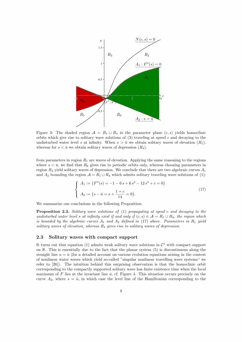
Figure 3: The shaded region A = R1 ∪ R4 in the parameter plane (c, s) yields homoclinicorbits which give rise to solitary wave solutions of (3) traveling at speed c and decaying to theundisturbed water level s at infinity. When s > u we obtain solitary waves of elevation (R1),whereas for s < u we obtain solitary waves of depression (R4).

from parameters in region R1 are waves of elevation. Applying the same reasoning to the regionswhere s < u, we find that R6 gives rise to periodic orbits only, whereas choosing parameters inregion R4 yield solitary waves of depression. We conclude that there are two algebraic curves A1

and A2 bounding the region A = R1 ∪R4 which admits solitary traveling wave solutions of (1):

A1 := F ′′(s) = −1− 6 s+ 6 s2 − 12 s3 + c = 0

A2 := s− u = s+1 + c

14= 0.

(17)

We summarize our conclusions in the following Proposition.

Proposition 2.3. Solitary wave solutions of (1) propagating at speed c and decaying to theundisturbed water level s at infinity exist if and only if (c, s) ∈ A = R1 ∪ R4, the region whichis bounded by the algebraic curves A1 and A2 defined in (17) above. Parameters in R1 yieldsolitary waves of elevation, whereas R4 gives rise to solitary waves of depression.

2.3 Solitary waves with compact support

It turns out that equation (1) admits weak solitary wave solutions in C1 with compact supporton R. This is essentially due to the fact that the planar system (5) is discontinuous along thestraight line u = u (for a detailed account on various evolution equations arising in the contextof nonlinear water waves which yield so-called ”singular nonlinear travelling wave systems“ werefer to [26]). The intuition behind this surprising observation is that the homoclinic orbitcorresponding to the compactly supported solitary wave has finite existence time when the localmaximum of F lies at the invariant line u, cf. Figure 4. This situation occurs precisely on thecurve A2, where s = u, in which case the level line of the Hamiltonian corresponding to the

8

homoclinic orbit based in the saddle point is hs = F (u) and F ′(u) = 0. Therefore, relation (8)simplifies to

v = ±√

2F (u)− F (u)

u− u = ±√

(u− u) p (u), (18)

where

p (u) := −F ′′(u)− 2

3!F (3)(u)(u− u)− · · · − 2

5!F (5)(u)(u− u)3.

In particular, the existence time of these homoclinic orbits is finite. Indeed, notice that

T (u, u0) :=

∫ u

u0

dr√(r − u) p(r)

is an elliptic integral and therefore finite, since p(r) is a third degree polynomial with no repeatedroots and u is not a root of p(r). In view of (18) this yields

T (u(ξ), u0) =

∫ u(ξ)

u(ξ0)

dr√(r − u)p(r)

=

∫ ξ

ξ0

√(u− u)p(u)√(u− u)p(u)

dξ = ξ − ξ0,

for a solution of u(ξ) =√

(u− u)p(u) with initial data u(ξ0) = u0. Hence, the time it takes anorbit to get from u to m, where m is the non-trivial solution of F (u) = F (m), is given by

T := T (u(ξ), u)− T (u(ξ),m) =

∫ m

u

dr√(r − u) p(r)

<∞.

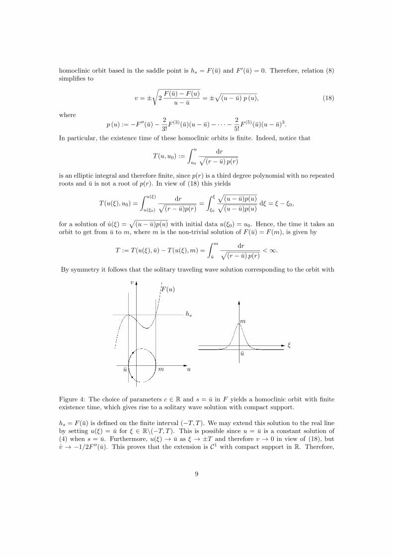
By symmetry it follows that the solitary traveling wave solution corresponding to the orbit with

F (u)

hs

uu m

u

m

v

ξ

Figure 4: The choice of parameters c ∈ R and s = u in F yields a homoclinic orbit with finiteexistence time, which gives rise to a solitary wave solution with compact support.

hs = F (u) is defined on the finite interval (−T, T ). We may extend this solution to the real lineby setting u(ξ) = u for ξ ∈ R\(−T, T ). This is possible since u = u is a constant solution of(4) when s = u. Furthermore, u(ξ) → u as ξ → ±T and therefore v → 0 in view of (18), butv → −1/2F ′′(u). This proves that the extension is C1 with compact support in R. Therefore,

9

u ∈ H1(R) is a weak solitary wave solution of (1) with compact support, see Remark 2.4. Noticethat, when ξ approaches ±T , the solution decays like

u(ξ) = u− 1

4F ′′(u)(ξ ± T )2 +O((ξ ± T )3) (19)

which is readily checked.

Remark 2.4. Equation (3) may be rewritten as

(1− c)u+ 3u2 − 2u3 + 3u4 − 7( d

dξu)2

= − 1

28

d2

dξ2

((1 + c+ 14u)2

)− 14K. (20)

We say that u ∈ H1loc(R) is a weak traveling wave solution of (1) if u satisfies (20) in the sense

of distributions. Observe that the weak formulation of equation (1) reads

ut + ∂x

(− u− 7u2 + (1− ∂2

x)−1(2u+ 10u2 − 2u3 + 3u4 − 7u2x))

= 0,

which is equivalent to (20) for periodic traveling waves, or traveling waves which decay at infinity.

2.4 Peaked periodic waves

For parameters in the regions R3 and R6, cf. Figure 3, the invariant line u lies between thetwo critical points of the polynomial F . In this case, the extrema of F yield two centers in thephase portrait of (6) which impedes the existence of solitary waves (and hence, the parameter sno longer accommodates the physical interpretation of the undisturbed water level at infinity).However, we show by continuous extension that there exist peaked periodic waves above andbelow the line u, and periodic waves undulating about u.

Indeed, for every (c, s) ∈ R3 ∪R6, periodic waves are obtained as in Proposition 2.1 by choosinghp ∈ (h1, h2), where hi = F (ui) for i = 1, 2, and ui is a solution of

F ′(y) = 0 and

F ′′(y) > 0 when y > u,F ′′(y) < 0 when y < u,

and employing (8). We will now treat the special case hp = F (u). Notice that, by construction,

hp − F (u) = (u− u)(u−m1)(u−m2) q(u),

where q(u) is a second order polynomial with no real roots and mi 6= u, i = 1, 2, are the othertwo intersections of the horizontal line hp with F (u). Using (8), we obtain two heteroclinic orbitsof the system (6) leaving and returning to the invariant line u = u given in terms of

vi = ±√

2 (u−m1)(u−m2) q(u), (21)

for u ∈ (m1, u) and u ∈ (u,m2) respectively, which intersect the horizontal axis at m1 and m2,where m1 < u < m2. Observe that for the topologically equivalent system (5), the existencetimes of these orbits are again finite and given in terms of

T1 =

∫ u

m1

du√2 (u−m1)(u−m2) q(u)

<∞

10

F (u)u

hp = F (u)

m1 m2u

v

ξ

ξ

ξ

(a) (b)

v1 v2

u1

u2

(b)

(c)

(a)

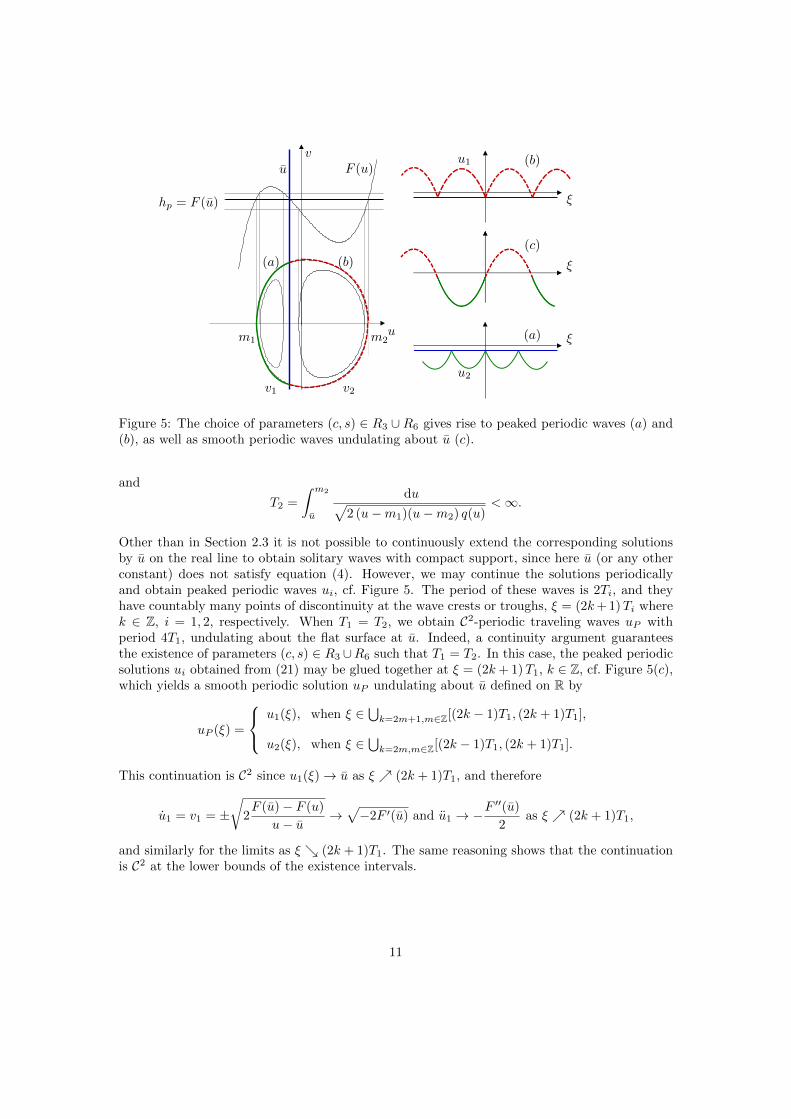
Figure 5: The choice of parameters (c, s) ∈ R3 ∪R6 gives rise to peaked periodic waves (a) and(b), as well as smooth periodic waves undulating about u (c).

and

T2 =

∫ m2

u

du√2 (u−m1)(u−m2) q(u)

<∞.

Other than in Section 2.3 it is not possible to continuously extend the corresponding solutionsby u on the real line to obtain solitary waves with compact support, since here u (or any otherconstant) does not satisfy equation (4). However, we may continue the solutions periodicallyand obtain peaked periodic waves ui, cf. Figure 5. The period of these waves is 2Ti, and theyhave countably many points of discontinuity at the wave crests or troughs, ξ = (2k+ 1)Ti wherek ∈ Z, i = 1, 2, respectively. When T1 = T2, we obtain C2-periodic traveling waves uP withperiod 4T1, undulating about the flat surface at u. Indeed, a continuity argument guaranteesthe existence of parameters (c, s) ∈ R3 ∪R6 such that T1 = T2. In this case, the peaked periodicsolutions ui obtained from (21) may be glued together at ξ = (2k+ 1)T1, k ∈ Z, cf. Figure 5(c),which yields a smooth periodic solution uP undulating about u defined on R by

uP (ξ) =

u1(ξ), when ξ ∈ ⋃k=2m+1,m∈Z[(2k − 1)T1, (2k + 1)T1],

u2(ξ), when ξ ∈ ⋃k=2m,m∈Z[(2k − 1)T1, (2k + 1)T1].

This continuation is C2 since u1(ξ)→ u as ξ (2k + 1)T1, and therefore

u1 = v1 = ±√

2F (u)− F (u)

u− u →√−2F ′(u) and u1 → −

F ′′(u)

2as ξ (2k + 1)T1,

and similarly for the limits as ξ (2k + 1)T1. The same reasoning shows that the continuationis C2 at the lower bounds of the existence intervals.

11

3 Properties of solitary traveling waves

The analysis in Section 2 shows that traveling wave solutions of (1) are symmetric with respectto the crest point, and that solitary waves tend (exponentially) to a constant on either side oftheir unique maximum or minimum. In the present Section, we will explore further propertiesregarding the shape of traveling waves. We determine how the wave amplitude, which is the pos-itive difference between crest and trough, changes with respect to the wave speed. Furthermore,we prove that traveling waves are strictly monotone between crest and trough.

3.1 Dependence of the amplitude on the wave speed

Our starting point is an algebraic expression for the change of a = m− s with respect to c.

Lemma 3.1. Let F be the polynomial defined in (9) and let (s,m) be a solution of

F ′(s) = 0,F (s)− F (m) = 0,

(22)

where s 6= u. Then, for a = m− s ∈ R, we have that

∂c a =−1/28

F ′(m)F ′′(s)

((s2 −m2)F ′′(s) + 2s F ′(m)

). (23)

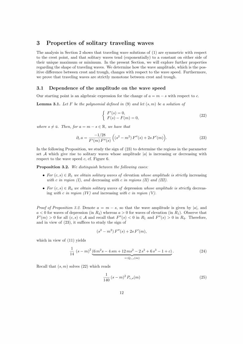
In the following Proposition, we study the sign of (23) to determine the regions in the parameterset A which give rise to solitary waves whose amplitude |a| is increasing or decreasing withrespect to the wave speed c, cf. Figure 6.

Proposition 3.2. We distinguish between the following cases:

• For (c, s) ∈ R1 we obtain solitary waves of elevation whose amplitude is strictly increasingwith c in region (I), and decreasing with c in regions (II) and (III).

• For (c, s) ∈ R4 we obtain solitary waves of depression whose amplitude is strictly decreas-ing with c in region (IV) and increasing with c in region (V).

Proof of Proposition 3.2. Denote a = m − s, so that the wave amplitude is given by |a|, anda < 0 for waves of depression (in R4) whereas a > 0 for waves of elevation (in R1). Observe thatF ′(m) > 0 for all (c, s) ∈ A and recall that F ′′(s) < 0 in R1 and F ′′(s) > 0 in R4. Therefore,and in view of (23), it suffices to study the sign of

(s2 −m2)F ′′(s) + 2s F ′(m),

which in view of (11) yields

1

14(s−m)

2(6m2s− 4 sm+ 12ms2 − 2 s2 + 6 s3 − 1 + c)︸ ︷︷ ︸

=:Qc,s(m)

. (24)

Recall that (s,m) solves (22) which reads

1

140(s−m)2 Pc,s(m) (25)

12

(I)

(III)

(II)

c∗

(IV )

(V )

c

s

A2 : s = u

A1 : F ′′(s) = 0

R(c, s) = 0

R1R4

Figure 6: Choosing parameters in the lighter shaded regions (I) and (V) we obtain solitarywaves which increase with the wave speed c, whereas solutions corresponding to parameters inthe darker shaded regions (II), (III) and (IV) decrease with respect to c.

where

Pc,s(m) := (6m3 − 5m2 + 12m2s+ 10m+ 18ms2 − 10 sm+ 5− 5 c− 15 s2 + 24 s3 + 20 s).

Since we are interested in solutions s 6= m, we study the system

Qc,s(m) = 0Pc,s(m) = 0

(26)

which has a solution if and only if Qc,s(m) and Pc,s(m) have a common root, i.e. if their resultantwith respect to m,

R(c, s) :=Res(Qc,s(m), Pc,s(m),m) (27)

= 31104 s9 − 10368 s8 + 32832 s7 + (−15552 c+ 39456) s6

+ (−3816− 864 c) s5 + (23472− 3312 c) s4 + 24 (c− 1) (108 c− 593) s3

+ 24 (33 c+ 107) (c− 1) s2 − 690 (c− 1)2s+ 36 (c− 1)

3,

is zero (see Appendix A.2 for a discussion on the involved curves). Hence, system (26) has asolution, i.e. ∂c a = 0, only along the algebraic curve R(c, s) = 0 meaning that within the regionsin A separated by this curve, the sign of ∂c a is constant. Hence, it suffices to pick one pair ofparameters (c, s) in each of these regions and compute the values of m and Q to determine thesign of ∂c a in view of expression (23). For example, let s1 = −0.1 and c1 = 1.5 in R1 then,computing the corresponding m1, we find that Qc1,s1(m1) > 0. Therefore, since F ′(m) < 0 andF ′′(s) < 0 in R1, we obtain that ∂c a > 0. Hence, the amplitude |a| of solitary wave solutions of(1) arising from parameters in the region denoted by (I) in Figure 6 is increasing with respectto the wave speed c. To provide an example for waves of depression, pick s4 = −0.5 and c4 = 15in R4, which yields m4 such that Qc4,s4(m4) < 0. Therefore, since F ′(m) < 0 and F ′′(s) > 0 inR4, we obtain that ∂c a > 0. In view of the fact that a < 0 in R4 this means that the amplitude

13

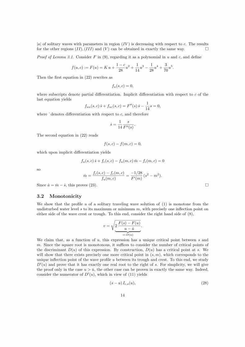
|a| of solitary waves with parameters in region (IV ) is decreasing with respect to c. The resultsfor the other regions (II), (III) and (V ) can be obtained in exactly the same way.

Proof of Lemma 3.1. Consider F in (9), regarding it as a polynomial in u and c, and define

f(u, c) := F (u) = K u+1− c

28u2 +

1

14u3 − 1

28u4 +

3

70u5.

Then the first equation in (22) rewrites as

fu(s, c) = 0,

where subscripts denote partial differentiation. Implicit differentiation with respect to c of thelast equation yields

fuu(s, c) s+ fuc(s, c) = F ′′(s) s− 1

14s = 0,

where ˙ denotes differentiation with respect to c, and therefore

s =1

14

s

F ′′(s).

The second equation in (22) reads

f(s, c)− f(m, c) = 0,

which upon implicit differentiation yields

fu(s, c) s+ fc(s, c)− fu(m, c) m− fc(m, c) = 0

so

m =fc(s, c)− fc(m, c)

fu(m, c)=−1/28

F ′(m)(s2 −m2).

Since a = m− s, this proves (23).

3.2 Monotonicity

We show that the profile u of a solitary traveling wave solution of (1) is monotone from theundisturbed water level s to its maximum or minimum m, with precisely one inflection point oneither side of the wave crest or trough. To this end, consider the right hand side of (8),

v =

√2F (s)− F (u)

u− u︸ ︷︷ ︸=:D(u)

.

We claim that, as a function of u, this expression has a unique critical point between s andm. Since the square root is monotonous, it suffices to consider the number of critical points ofthe discriminant D(u) of this expression. By construction, D(u) has a critical point at s. Wewill show that there exists precisely one more critical point in (s,m), which corresponds to theunique inflection point of the wave profile u between its trough and crest. To this end, we studyD′(u) and prove that it has exactly one real root to the right of s. For simplicity, we will givethe proof only in the case u > u, the other case can be proven in exactly the same way. Indeed,consider the numerator of D′(u), which in view of (11) yields

(s− u) Ic,s(u), (28)

14

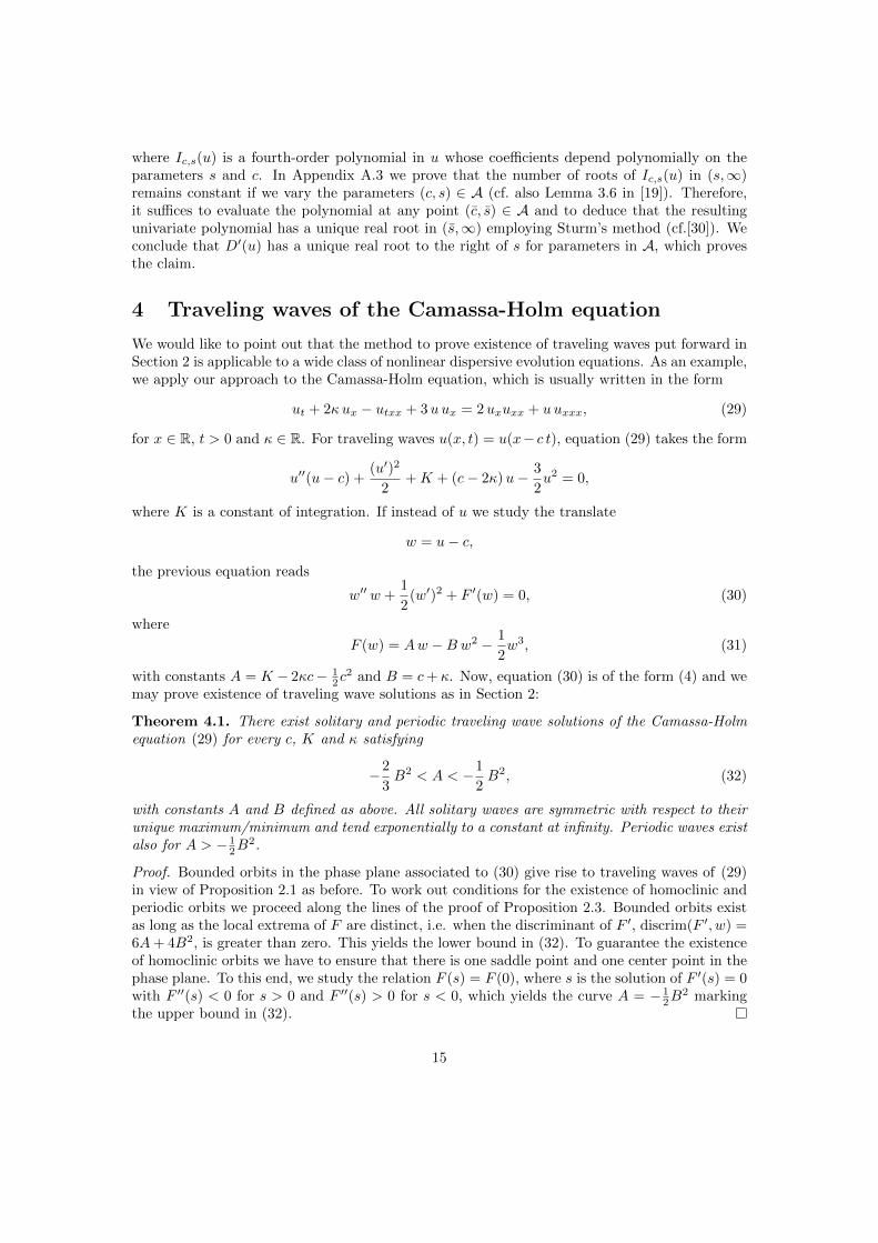
where Ic,s(u) is a fourth-order polynomial in u whose coefficients depend polynomially on theparameters s and c. In Appendix A.3 we prove that the number of roots of Ic,s(u) in (s,∞)remains constant if we vary the parameters (c, s) ∈ A (cf. also Lemma 3.6 in [19]). Therefore,it suffices to evaluate the polynomial at any point (c, s) ∈ A and to deduce that the resultingunivariate polynomial has a unique real root in (s,∞) employing Sturm’s method (cf.[30]). Weconclude that D′(u) has a unique real root to the right of s for parameters in A, which provesthe claim.

4 Traveling waves of the Camassa-Holm equation

We would like to point out that the method to prove existence of traveling waves put forward inSection 2 is applicable to a wide class of nonlinear dispersive evolution equations. As an example,we apply our approach to the Camassa-Holm equation, which is usually written in the form

ut + 2κux − utxx + 3uux = 2uxuxx + uuxxx, (29)

for x ∈ R, t > 0 and κ ∈ R. For traveling waves u(x, t) = u(x− c t), equation (29) takes the form

u′′(u− c) +(u′)2

2+K + (c− 2κ)u− 3

2u2 = 0,

where K is a constant of integration. If instead of u we study the translate

w = u− c,

the previous equation reads

w′′ w +1

2(w′)2 + F ′(w) = 0, (30)

where

F (w) = Aw −Bw2 − 1

2w3, (31)

with constants A = K − 2κc− 12c

2 and B = c+ κ. Now, equation (30) is of the form (4) and wemay prove existence of traveling wave solutions as in Section 2:

Theorem 4.1. There exist solitary and periodic traveling wave solutions of the Camassa-Holmequation (29) for every c, K and κ satisfying

−2

3B2 < A < −1

2B2, (32)

with constants A and B defined as above. All solitary waves are symmetric with respect to theirunique maximum/minimum and tend exponentially to a constant at infinity. Periodic waves existalso for A > − 1

2B2.

Proof. Bounded orbits in the phase plane associated to (30) give rise to traveling waves of (29)in view of Proposition 2.1 as before. To work out conditions for the existence of homoclinic andperiodic orbits we proceed along the lines of the proof of Proposition 2.3. Bounded orbits existas long as the local extrema of F are distinct, i.e. when the discriminant of F ′, discrim(F ′, w) =6A+ 4B2, is greater than zero. This yields the lower bound in (32). To guarantee the existenceof homoclinic orbits we have to ensure that there is one saddle point and one center point in thephase plane. To this end, we study the relation F (s) = F (0), where s is the solution of F ′(s) = 0with F ′′(s) < 0 for s > 0 and F ′′(s) > 0 for s < 0, which yields the curve A = − 1

2B2 marking

the upper bound in (32).

15

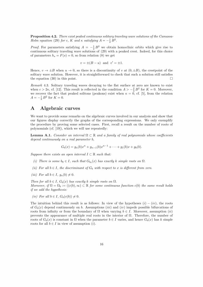
Proposition 4.2. There exist peaked continuous solitary traveling wave solutions of the Camassa-Holm equation (29) for c, K and κ satisfying A = − 1

2 B2.

Proof. For parameters satisfying A = − 12 B

2 we obtain homoclinic orbits which give rise tocontinuous solitary traveling wave solutions of (29) with a peaked crest. Indeed, for this choiceof parameters hs = F (s) = 0, so from relation (8) we get

v = ±(B − u) and v′ = ±1.

Hence, v → ±B when u → 0, so there is a discontinuity of v at (0,±B), the crestpoint of thesolitary wave solution. However, it is straightforward to check that such a solution still satisfiesthe equation (30) in this point.

Remark 4.3. Solitary traveling waves decaying to the flat surface at zero are known to existwhen c > 2κ, cf. [12]. This result is reflected in the condition A > − 2

3 B2 for K = 0. Moreover,

we recover the fact that peaked solitons (peakons) exist when κ = 0, cf. [5], from the relationA = − 1

2 B2 for K = 0.

A Algebraic curves

We want to provide some remarks on the algebraic curves involved in our analysis and show thatour figures display correctly the graphs of the corresponding expressions. We only exemplifythe procedure by proving some selected cases. First, recall a result on the number of roots ofpolynomials (cf. [19]), which we will use repeatedly:

Lemma A.1. Consider an interval Ω ⊂ R and a family of real polynomials whose coefficientsdepend continuously on a real parameter b,

Gb(x) = gn(b)xn + gn−1(b)xn−1 + · · ·+ g1(b)x+ g0(b).

Suppose there exists an open interval I ⊂ R such that:

(i) There is some b0 ∈ I, such that Gb0(x) has exactly k simple roots on Ω.

(ii) For all b ∈ I, the discriminant of Gb with respect to x is different from zero.

(iii) For all b ∈ I, gn(b) 6= 0.

Then for all b ∈ I, Gb(x) has exactly k simple roots on Ω.Moreover, if Ω = Ωb := ((c(b),∞) ⊂ R for some continuous function c(b) the same result holdsif we add the hypothesis:

(iv) For all b ∈ I, Gb(c(b)) 6= 0.

The intuition behind this result is as follows: In view of the hypotheses (i) − (iv), the rootsof Gb(x) depend continuously on b. Assumptions (iii) and (iv) impede possible bifurcations ofroots from infinity or from the boundary of Ω when varying b ∈ I. Moreover, assumption (ii)prevents the appearance of multiple real roots in the interior of Ω. Therefore, the number ofroots of Gb(x) is constant in Ω when the parameter b ∈ I varies, and hence Gb(x) has k simpleroots for all b ∈ I in view of assumption (i).

16

A.1 On the curves in Section 2.2

We have to ensure that the algebraic curve M(c, s) = 0 in (14) has no real roots, and that N(c, s)in (15) has a unique root for every choice of parameters (c, s). Furthermore, we want to showthat the curves N(c, s) = 0 and A1, A2 of (17) all intersect in precisely one point. We have

M(c, s) = 243 c2 +(−900 s− 778 + 540 s2 − 1080 s3

)c

+ 823 + 1284 s+ 480 s2 + 480 s3 + 2700 s4 − 1296 s5 + 1296 s6,

which we regard as a polynomial in c with parameter s. To show that it has no real roots, wecheck that the conditions of Lemma A.1 are satisfied for k = 0. Assumption (iii) holds, sincethe coefficient of the highest order term is constant. Computing the discriminant of M(c, s) withrespect to c yields

−16(18 s2 − 6 s+ 23

)3,

for which it is straightforward to prove that it has no zeros in R. To check assumption (i) wechoose, for example, s = −1 which gives

M(c,−1) = 243 c2 + 1742 c+ 4831 > 0.

In view of Lemma A.1, we find that M(c, s) is strictly positive for all c, s ∈ R. Next we focus on

N(c, s) = 3 c3 + (−42 s+ 37) c2 +(−476 s+ 588 s2 + 3397

)c

+ 6076 s2 − 8232 s3 − 8666 s− 2125.

It is straightforward to show that assumptions (ii) and (iii) hold. Regarding (i), we choose forexample s = 1 and find that

N(c, 1) = (3c− 11) (c2 + 2c+ 1177)

which clearly has a unique root. Hence, for each s ∈ R there exists precisely one c ∈ R suchthat N(c, s) = 0. To prove that the curves A1, A2 and N(c, s) = 0 all intersect in precisely onepoint, observe that the Ai are linear in c and it is therefore easy to check that they intersect at apoint (c∗, s∗) where s∗ is the root of the cubic polynomial P∗ := −2− 20 s+ 6 s2 − 12 s3 and c∗,the corresponding value on the curve A2, is given by the unique real solution of the polynomial3 c3 + 30 c2 + 1031 c− 368 = 0 as stated in Theorem 1.1. To see that N(c, s) = 0 also intersectsin that point, compute the resultant of A2 and N with respect to c and find that the resultingpolynomial is just a factor of PI which proves the claim.

A.2 On the curves in Section 3.1

In this subsection, we want to discuss the curves in (24), (25) and (27). We show that the curveR(c, s) = 0 intersects the curve A2 three times whereas it intersects A1 only once, which yieldsthe different regions depicted in Figure 6. To prove the latter result, we solve both A1 and A2

for c and plug the resulting expressions into R(c, s). We obtain univariate polynomials in s forwhich it is straightforward to show that they have three roots (two negative and one positive) andone root (in zero), respectively. To show that the polynomial expressions defining the involvedcurves yield a unique root for each (c, s) ∈ R2, we again employ Lemma A.1 and check that theassumptions are satisfied. We exemplify the procedure by showing that the result is true for thecurve Pc,s(m) = 0, where

Pc,s(m) =− 6m3 + (5− 12 s)m2 + (−18 s2 + 10 s− 10)m

− 24 s3 + 15 s2 − 20 s− 5 + 5 c.

17

Note that we are now dealing with a polynomial which depends on two parameters. Assumption(iii) holds in view of the fact that the coefficient of the highest order term is constant, and itis straightforward to check (i) choosing parameters (c, s) which yield that Pc,s(m) has preciselyone root. To prove assumption (ii), we compute the discriminant of Pc,s(m) with respect to mand obtain

Dis(Pc,s(m),m) = −24300 c2 + (120600 s− 75600 s2 + 73100 + 151200 s3)c

− 70300− 96200 s2 − 163600 s− 504000 s4 + 259200 s5 + 2400 s3 − 259200 s6.

To show that Discrim(Pc,s(m)) is different from zero, we repeat the scheme for this polynomialin c with parameter s and ensure again that the assumptions of Lemma A.1 hold with k = 0.

A.3 On the curves in Section 3.2

The goal of this subsection is to prove that for the polynomial

Ic,s(u) =− 168u4 + (90− 15 c− 168 s)u3 +(10 c− 130− 168 s2 + 90 s− 15 sc

)u2

+ (−50 + 10 sc+ 20 c− 130 s+ 90 s2 − 168 s3 − 15 s2c)u

− 5− 50 s+ 90 s3 + 5 c2 + 20 sc− 130 s2 − 168 s4 + 10 s2c− 15 s3c,

obtained in (28), the number of roots do not change if we vary the parameters (c, s) in theadmissible region A. We will again employ Lemma A.1 above for I = A and Ωc,s = (s,∞).Indeed, assumption (iii) holds since the highest coefficient of Ic,s(u) is constant. To check that(iv) is satisfied, we evaluate the polynomial at u = s and find that

Ic,s(s) = (s− u)F ′′(s).

These factors are exactly the relations which bound the admissible parameter region A, andhence they do not vanish in the interior of A. Note, however, that solitary waves with compactsupport arise from a choice of parameters (c, s) on the curve A2 = s − u = 0, so we need aseparate argument in that case which will be carried out below. Next we study the discriminantof Ic,s(u) with respect to u,

Dis(Ic,s(u), u) = D1(c, s)D2(c, s), (33)

and claim that the algebraic curves corresponding to the zeros of these factors lie outside ofA. To see this, observe that the curves A1, A2, D1(c, s) = 0 and D2(c, s) = 0 in-tersect precisely once in the point (c∗, s∗). Then, we choose some c1 < c∗ and find thatD1(c1, s) > A1(c1, s) > A2(c1, s) > D2(c1, s), whereas for any c2 > c∗ we obtain the reverseorder. Hence, the discriminant of Ic,s(u) does not vanish in A, which proves the claim. There-fore, the assumptions of Lemma A.1 hold, and we find that the number of roots of Ic,s(u) isconstant in the interior of A.

We now provide a separate but similar argument which asserts that this result holds also forparameters on the curve A2. Indeed, for (c, s) on A2, i.e. when s = u, we find that

D′(u) = Ic(u),

where Ic(u) is a cubic polynomial in u whose coefficients depend polynomially on c. Along thelines of the above proof we argue that Ic(u) has a unique real root in (u,∞). Indeed, no bi-furcations of roots occur at infinity, and evaluating Ic(u) at the boundary u = u yields a cubic

18

polynomial in c which vanishes only in c∗ /∈ A. Using Sturm’s method (cf.[30]) we show that thediscriminant of Ic(u) with respect to u does not vanish. Hence, the number of roots is constant,and choosing any c we find that Ic(u) has a unique real root in (uc,∞).

We conclude with a discussion of the polynomials in (33),

D1 =− 32928 s3 + (1764 c+ 22344)s2 − (84 c2 + 1148 c+ 28504)s

+ 3 c3 + 44 c2 + 7919 c− 5842

and

D2 = 30375 c5 + (67500 s2 − 135000 s3 + 93100 + 567900 s)c4

+ (2083200 s2 − 3518100 s4 + 408900 s+ 162000 s6 + 1280400 s3 − 162000 s5 + 880703)c3

+ (−368064 s− 4730400 s6 − 8347536 s2 + 5443200 s7 + 6777000 s4 − 11014128 s3

− 25691040 s5 − 3605574)c2 + (−44997120 s7 + 4400084− 15110352 s+ 23678784 s5

− 9163584 s6 + 60963840 s8 − 22971024 s2 − 17525952 s3 − 58261680 s4)c+ 227598336 s9

− 138184704 s8 + 31667136 s+ 301625856 s7 + 71568192 s3 + 152350848 s6 + 1062232

+ 54393984 s5 + 49720800 s2 + 187454304 s4.

We will only discuss the latter curve and employ Lemma A.1 again for I × Ω = A. Note thatassumption (iii) holds in view of the fact that the coefficient of the highest order term is constant.Computing the discriminant with respect to c yields

Dis(D2, c) =α0 (11664000 s12 − 23328000 s11 + 367804800 s10 − 487728000 s9

+ 3390049800 s8 − 2253805200 s7 + 4960871884 s6 + 2160459976 s5

+ 1280057526 s4 + 4059678628 s3 + 1729573411 s2 + 1328288220 s+ 695918709)

× (84672 s4 + 22512 s3 + 76402 s2 + 58822 s+ 16767)3

× (16767 + 29606 s− 12083 s2 − 4040 s3 + 20160 s4

︸ ︷︷ ︸=:D(s)

)2,

where α0 > 0 is a real constant. It is straightforward to see that the first two factors of theabove expression have no real roots, whereas the last factor D(s) vanishes for two values s1 ands2, meaning that D2(c, si) may have multiple roots in that case. To ensure that assumption (ii)holds, we have to prove that these values do not lie in A. To this end, we use Sturm’s methodto derive rational upper and lower bounds for si such that s1 ∈ [s1, s1] and s2 ∈ [s2, s2], tobound the curves Ai from above and below by rational constants. For example, we find thats1 ∈ [− 131

128 ,− 6564 ] =: I1. We claim that all values of D2 in the strip defined by I1 lie outside of

A. To this end we compute a bound for A2,

M1 := mins∈I1c ∈ R : A(c, s) = 0 =

423

32∈ Q,

and construct a rational univariate polynomial

D2(c) = 30375 c5 − 8897979325

32768c4 − 602652229378808443

274877906944c3

+3196448247290763459

137438953472c2 +

2641868472255829530863

70368744177664c

− 17460388511693021202337

35184372088832,

19

using the upper and lower bounds of the interval I1 such that D2(c, s) < D2(c). Then, it is fairlystraightforward to see that D2(c, s)−M1 < D2(c)−M1 < 0, which proves the claim. Repeatingthis procedure with the root s2 and the other bounding curves Ai shows that in the region A allinvolved curves are displayed correctly.

Acknowledgements

The first author is partially supported by a MCYT- FEDER grant number MTM2008-03437 andby a CIRIT grant number 2009SGR 410. The second author is supported by the FWF projectJ3452 ”Dynamical Systems Methods in Hydrodynamics“ of the Austrian Science Fund.

References

[1] A. Boutet de Monvel, A. Kostenko, D. Shepelsky, and G. Teschl. Long-time asymptoticsfor the Camassa-Holm equation. SIAM J. Math. Anal., 41(4):1559–1588, 2009.

[2] A. Bressan and A. Constantin. Global conservative solutions of the Camassa-Holm equation.Arch. Ration. Mech. Anal., 183:215–239, 2007.

[3] A. Bressan and A. Constantin. Global Dissipative Solutions of the Camassa–Holm Equation.Anal. Appl., 5(1):1–27, 2007.

[4] R. Camassa and D. D. Holm. An integrable shallow water equation with peaked solitons.Phys. Rev. Lett., 71(11):1661–1664, 1993.

[5] R. Camassa, D. D. Holm, and J. M. Hyman. A new integrable shallow water equation. Adv.Appl. Mech., 31(31):1–33, 1994.

[6] A. Constantin. On the scattering problem for the Camassa-Holm equation. Proc. Roy. Soc.London Ser. A, 457:953–970, 2001.

[7] A. Constantin. Nonlinear Water Waves with Applications to Wave-Current Interactionsand Tsunamis. CBMS-NSF R SIAM, Philadelphia, 2011.

[8] A. Constantin and J. Escher. Wave breaking for nonlinear nonlocal shallow water equations.Acta Math., 181(2):229–243, 1998.

[9] A. Constantin and J. Escher. Well-posedness, global existence and blowup phenomena fora periodic quasi-linear hyperbolic equation. Comm. Pure Appl. Math., LI:475–504, 1998.

[10] A. Constantin, V. S. Gerdjikov, and R. I. Ivanov. Inverse scattering transform for theCamassa-Holm equation. Inverse Probl., 22(6):2197–2207, 2006.

[11] A. Constantin and D. Lannes. The hydrodynamical relevance of the Camassa-Holm andDegasperis-Procesi equations. Arch. Ration. Mech. Anal., 192:165–186, 2009.

[12] A. Constantin and W. Strauss. Stability of the Camassa-Holm solitons. J. Nonlinear Sci.,12(4):415–422, 2002.

[13] F. Dumortier, J. Llibre, and J. C. Artes. Qualitative Theory of Planar Differential Systems.Springer, Berlin, 2006.

20

[14] N. Duruk Mutlubas. Local well-posedness and wave breaking results for periodic solutionsof a shallow water equation for waves of moderate amplitude. Nonlinear Anal. Theory,Methods Appl., to appear, 2013.

[15] N. Duruk Mutlubas. On the Cauchy problem for a model equation for shallow water wavesof moderate amplitude. Nonlinear Anal. Real World Appl., 14(5):2022–2026, 2013.

[16] N. Duruk Mutlubas and A. Geyer. Orbital stability of solitary waves of moderate amplitudein shallow water. J. Differ. Equations, 255(2):254–263, 2013.

[17] N. Duruk Mutlubas, A. Geyer, and B.-V. Matioc. Non-uniform continuity of the flow mapfor an evolution equation modeling shallow water waves of moderate amplitude. NonlinearAnal. Real World Appl., to appear, 2013.

[18] K. El Dika and L. Molinet. Exponential decay of H1-localized solutions and stability of thetrain of N solitary waves for the Camassa-Holm equation. Philos. Trans. Roy. Soc. LondonSer. A, 365(1858):2313–31, 2007.

[19] A. Gasull, H. Giacomini, and J. D. Garcıa-Saldana. Bifurcation values for a family of planarvector fields of degree five. arXiv:1202.1919v1, 2012.

[20] A. Geyer. Solitary traveling water waves of moderate amplitude. J. Nonl. Math. Phys.,19(supp.01):1240010, 12 p., 2012.

[21] M. Grillakis, J. Shatah, and W. Strauss. Stability theory of solitary waves in the presenceof symmetry I. J. Funct. Anal., 74(1):160–197, 1987.

[22] J. Guggenheimer and P. Holmes. Nonlinear Oscillations, Dynamical Systems, and Bifurca-tions of Vector Fields. Springer, 1983.

[23] R. S. Johnson. Camassa-Holm, Korteweg-de Vries and related models for water waves. J.Fluid Mech., 455:63–82, 2002.

[24] T. Kato. Quasi-linear equations of evolution, with applications to partial differential equa-tions. Spectr. Theory Differ. Equations, 448:25–70, 1975.

[25] J. Lenells. Traveling wave solutions of the Camassa–Holm equation. J. Differ. Equations,217(2):393–430, 2005.

[26] J. Li. Singular Nonlinear Travelling Wave Equations: Bifurcations and Exact Solutions.Science Press, Mathematics Monograph Series 27, Beijing, 2013.

[27] Y. Mi and C. Mu. On the solutions of a model equation for shallow water waves of moderateamplitude. J. Differ. Equations, 255(8):2101–2129, 2013.

[28] L. Perko. Differential Equations and Dynamical Systems. Springer, New York, 2006.

[29] J. Sotomayor. Licoes de Equacoes Diferenciais Ordinarias. Projeto Euclides, 11. Institutode Matematica Pura e Aplicada, Rio de Janeiro, 1979.

[30] J. Stoer and R. Bulirsch. Introduction to numerical analysis. Springer Verlag, New YorkHeidelberg, 1980.

[31] G. Teschl. Ordinary Differential Equations and Dynamical Systems. Graduate Studies inMathematics, 140. AMS, Providence, RI, 2012.

21