Traveling Salesman with Deadlines

Adam Meyerson

UCLA

Acknowledgements

• Orienteering Results– Joint with Avrim Blum, Shuchi Chawla, David

Karger, Terran Lane, Maria Minkoff– FOCS 2003

• TSP with Deadlines– Joint with Nikhil Bansal, Avrim Blum, Shuchi

Chawla– STOC 2004

Problem Statement

• We are given various points where deliveries must be made, along with a deadline for each delivery. The goal is to find a path which makes as many deliveries as possible by their deadlines.

• This is a simplification of the problem of vehicle routing with time windows. In fact, we can add release times to model this exactly.

Motivation/Applications

• Vehicle Routing with Time Windows named as one of the most important problems in operations research.

• Robot Navigation!

• Task scheduling with setup times.

• Orienteering a long-standing open problem in approximation algorithms.

Related Problems

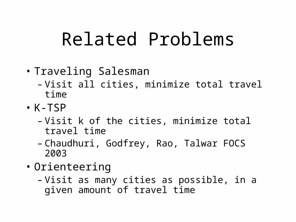
• Traveling Salesman– Visit all cities, minimize total travel time

• K-TSP– Visit k of the cities, minimize total travel time– Chaudhuri, Godfrey, Rao, Talwar FOCS 2003

• Orienteering– Visit as many cities as possible, in a given

amount of travel time

Minimum Excess Path

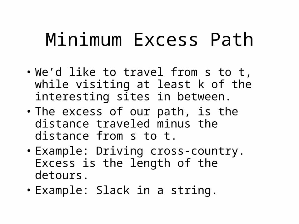
• We’d like to travel from s to t, while visiting at least k of the interesting sites in between.

• The excess of our path, is the distance traveled minus the distance from s to t.

• Example: Driving cross-country. Excess is the length of the detours.

• Example: Slack in a string.

Solution Concept

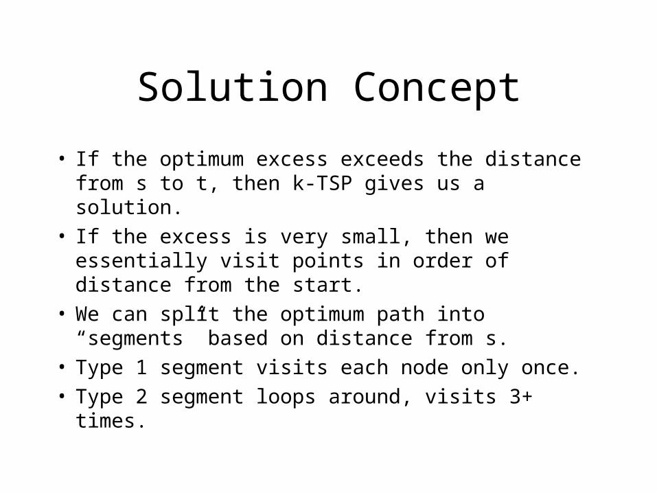
• If the optimum excess exceeds the distance from s to t, then k-TSP gives us a solution.

• If the excess is very small, then we essentially visit points in order of distance from the start.

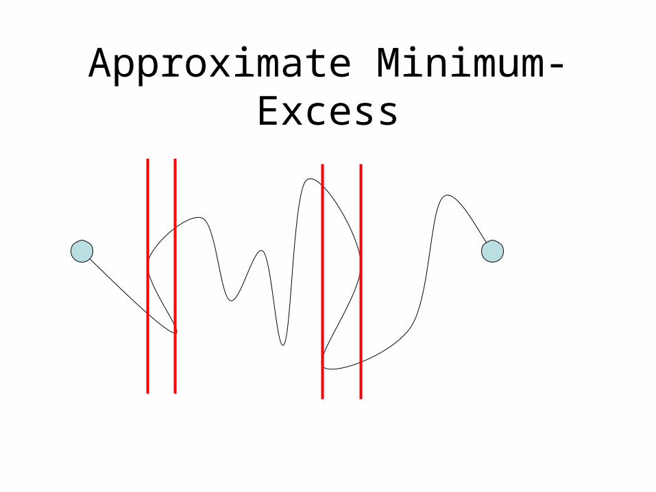
• We can split the optimum path into “segments” based on distance from s.

• Type 1 segment visits each node only once.• Type 2 segment loops around, visits 3+ times.

Approximate Minimum-Excess

Algorithm for Min-Excess

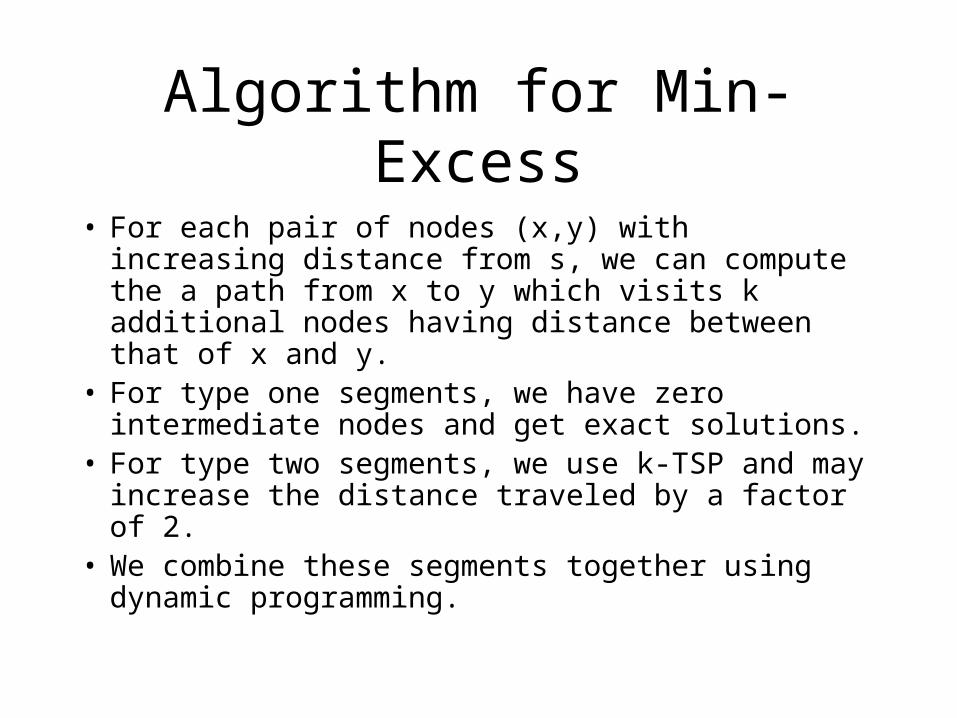
• For each pair of nodes (x,y) with increasing distance from s, we can compute the a path from x to y which visits k additional nodes having distance between that of x and y.

• For type one segments, we have zero intermediate nodes and get exact solutions.

• For type two segments, we use k-TSP and may increase the distance traveled by a factor of 2.

• We combine these segments together using dynamic programming.

Analysis of Min-Excess

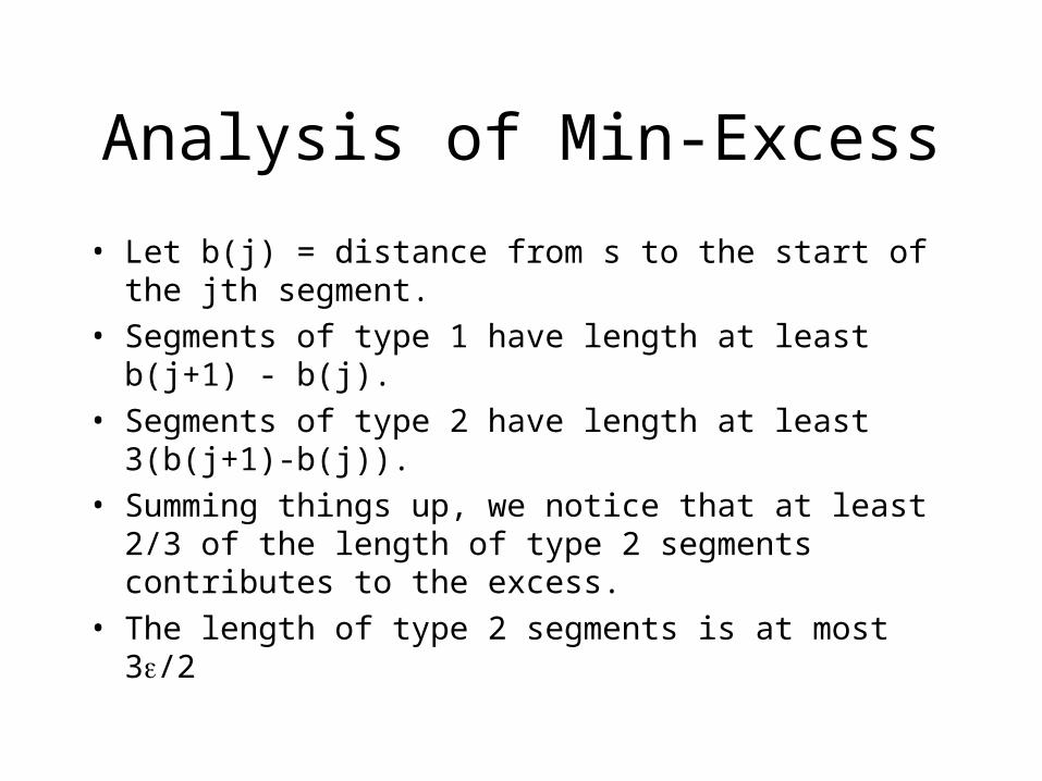
• Let b(j) = distance from s to the start of the jth segment.

• Segments of type 1 have length at least b(j+1) - b(j).

• Segments of type 2 have length at least 3(b(j+1)-b(j)).

• Summing things up, we notice that at least 2/3 of the length of type 2 segments contributes to the excess.

• The length of type 2 segments is at most 3/2

Min-Excess Result

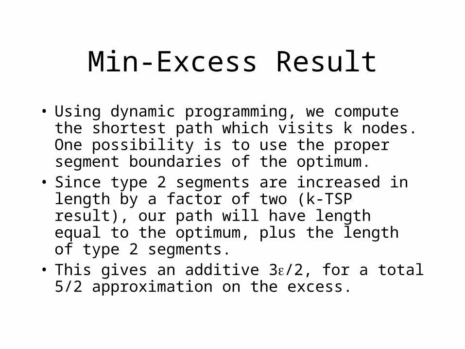
• Using dynamic programming, we compute the shortest path which visits k nodes. One possibility is to use the proper segment boundaries of the optimum.

• Since type 2 segments are increased in length by a factor of two (k-TSP result), our path will have length equal to the optimum, plus the length of type 2 segments.

• This gives an additive 3/2, for a total 5/2 approximation on the excess.

Point-to-Point Orienteering

• Given a pair of points (u,v) and a distance bound D. We’d like to travel from u to v while visiting as many intermediate nodes as possible. However, we are required to reach v by time D.

Point to Point Algorithm

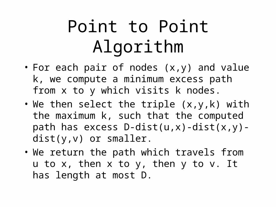
• For each pair of nodes (x,y) and value k, we compute a minimum excess path from x to y which visits k nodes.

• We then select the triple (x,y,k) with the maximum k, such that the computed path has excess D-dist(u,x)-dist(x,y)-dist(y,v) or smaller.

• We return the path which travels from u to x, then x to y, then y to v. It has length at most D.

Properties of Excess

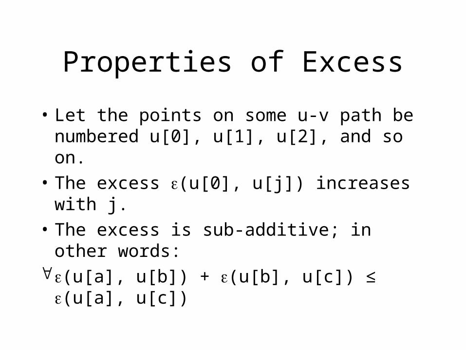
• Let the points on some u-v path be numbered u[0], u[1], u[2], and so on.

• The excess (u[0], u[j]) increases with j.

• The excess is sub-additive; in other words:(u[a], u[b]) + (u[b], u[c]) ≤ (u[a], u[c])

Point to Point Analysis

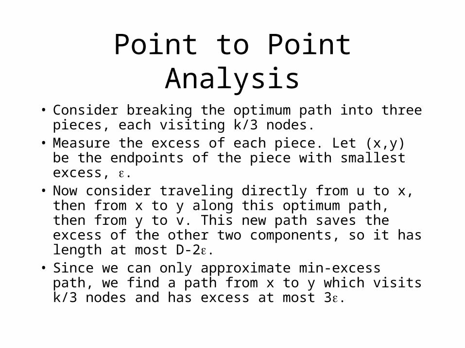
• Consider breaking the optimum path into three pieces, each visiting k/3 nodes.

• Measure the excess of each piece. Let (x,y) be the endpoints of the piece with smallest excess, .

• Now consider traveling directly from u to x, then from x to y along this optimum path, then from y to v. This new path saves the excess of the other two components, so it has length at most D-2.

• Since we can only approximate min-excess path, we find a path from x to y which visits k/3 nodes and has excess at most 3.

Multiple Deadlines

• We now consider the multiple deadline problem. Each node x which we might visit has its own deadline D(x). Our goal is to visit as many nodes as possible before their respective deadlines.

• Note that orienteering is the case where the deadlines of all nodes are equal D(x)=D.

Small Margin Case

• Suppose most nodes x are visited between D(x)/1+ and D(x). In other words, most of the value comes from visiting nodes very close to their deadline.

• Intuitively, this means we are “almost” visiting nodes in order of deadline.

Small Margin Algorithm

• For each (j,x,y) we will find a path from x to y which visits as many nodes as possible which have deadlines between (1+)^j and (1+)^(j+2).

• This path should have length at most (1+)^j• We will paste these segments together to

maximize the number of nodes visited.• Again we use dynamic programming.

Small Margin Analysis

• The segment represents the points visited between time (1+)^j and (1+)^(j+1). Since the optimum visits only nodes with the appropriate deadlines, we can will find a way to visit at least OPT/3 nodes.

• However, some nodes may be visited multiple times. This is at most twice though.

• Also, some deadlines may be exceeded, but only by a factor of (1+).

Large Margin Case

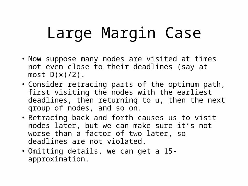
• Now suppose many nodes are visited at times not even close to their deadlines (say at most D(x)/2).

• Consider retracing parts of the optimum path, first visiting the nodes with the earliest deadlines, then returning to u, then the next group of nodes, and so on.

• Retracing back and forth causes us to visit nodes later, but we can make sure it’s not worse than a factor of two later, so deadlines are not violated.

• Omitting details, we can get a 15-approximation.

Bicriteria Approximation

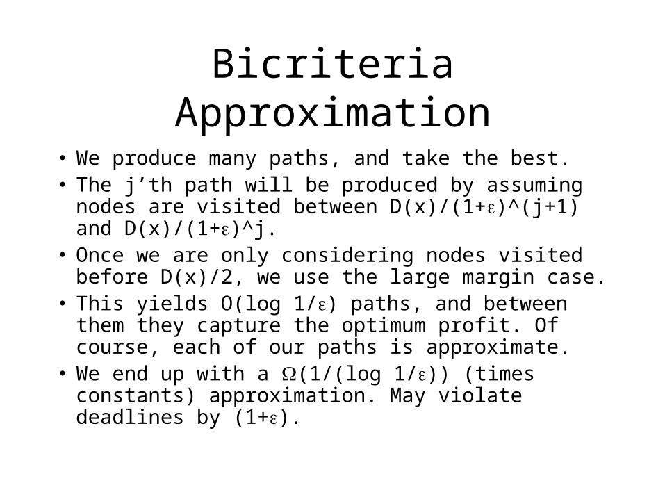
• We produce many paths, and take the best.• The j’th path will be produced by assuming nodes are

visited between D(x)/(1+)^(j+1) and D(x)/(1+)^j. • Once we are only considering nodes visited before

D(x)/2, we use the large margin case.• This yields O(log 1/) paths, and between them they

capture the optimum profit. Of course, each of our paths is approximate.

• We end up with a (1/(log 1/)) (times constants) approximation. May violate deadlines by (1+).

O(log n) Approximation

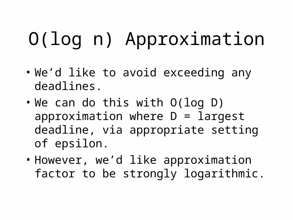
• We’d like to avoid exceeding any deadlines.

• We can do this with O(log D) approximation where D = largest deadline, via appropriate setting of epsilon.

• However, we’d like approximation factor to be strongly logarithmic.

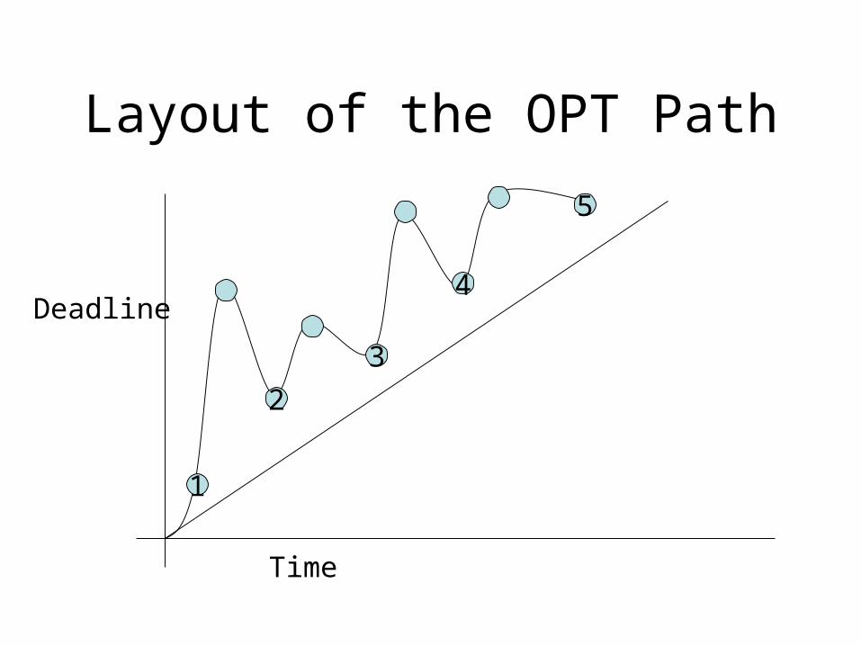
Layout of the OPT Path

Time

Deadline

5

4

3

2

1

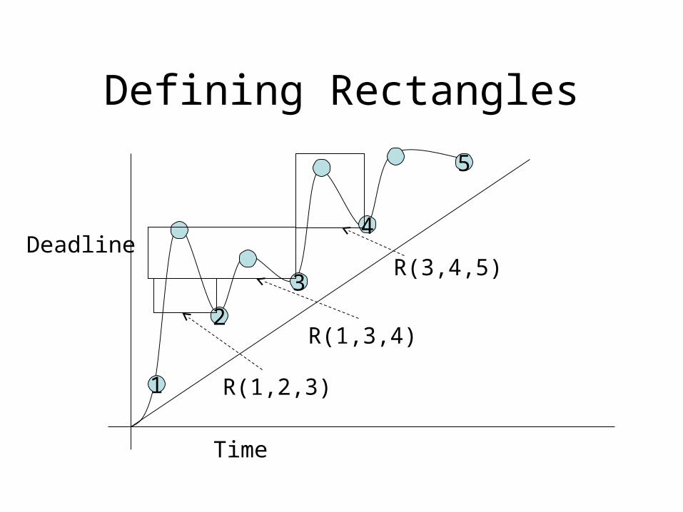
Defining Rectangles

Time

Deadline

5

4

3

2

1 R(1,2,3)

R(1,3,4)

R(3,4,5)

Rectangle Definition

• A rectangle R(a,b,c) has its left edge at the time OPT visits a, its top at the deadline of point c, and its lower right corner at point b. These points are all in the lower envelope.

• Two rectangles are disjoint if no vertical or horizontal line intersects both of them.

• A collection of disjoint rectangles is a collection of rectangles which are pairwise disjoint.

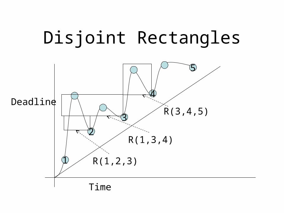
Disjoint Rectangles

Time

Deadline

5

4

3

2

1 R(1,2,3)

R(1,3,4)

R(3,4,5)

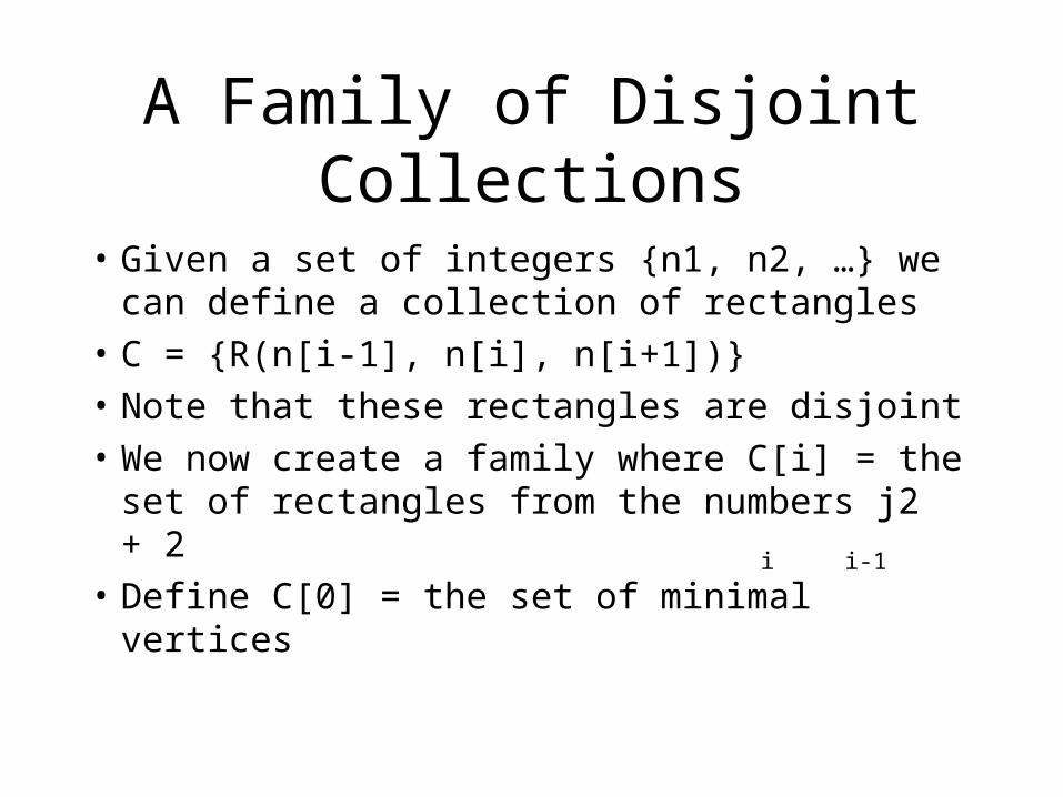
A Family of Disjoint Collections

• Given a set of integers {n1, n2, …} we can define a collection of rectangles

• C = {R(n[i-1], n[i], n[i+1])}

• Note that these rectangles are disjoint

• We now create a family where C[i] = the set of rectangles from the numbers j2 + 2

• Define C[0] = the set of minimal vertices

i i-1

Every Node in OPT is in Family

• Consider a vertex v visited by OPT• Let D(v[i]) ≤ D(v) ≤ D(v[i+1]) for some i• Let t(v[j-1]) ≤ t(v) ≤ t(v[j]) for some j• Observe that i ≥ j• If i=j, then v is a minimal vertex (in C[0])• Otherwise, i and j both lie in a rectangle of C[b] if the

corresponding set contains exactly one number between [i, j]

• Select b such that 2 ≤ i-j ≤ 2• Now v is in either C[b] or C[b+1]

b b+1

Approximating the Best C[b]

• Consider restricting OPT to just one collection C[b]. Since each rectangle contains a set of points with distinct deadlines, if we could run point-to-point orienteering on the rectangles we’d be done.

• But we don’t know which are the minimal vertices, and thus don’t know the rectangles.

Dynamic Program

• We arrange the vertices in increasing order of deadline.

• For each j,k we consider the graph restricted to vertices with deadlines between the jth and kth deadline.

• We then solve point-to-point orienteering, requiring that each vertex be visited before deadline D(j).

Algorithm Details

• Let π(j,k,g,h,p) = Point to point solution starting at g and ending at h, obtaining profit only for vertices with deadlines between D(j) and D(k). The “start time” at vertex g is the earliest time such that we can obtain profit p for nodes with deadlines before D(j) by the time we reach g. The “finish time” for orienteering is D(j).

• Note that assuming we can compute the start time, all of these can be determined using P2P orienteering.

More Details

• Now we compute (k, p, g) = minimum length path which obtains at least reward p from visiting nodes with deadline at most D(k) and has path end at g.

• This can be computed as:(k, p, g) = min (j, q, h)+π(j,k,h,g,p-q) • Note that the start time for π(j,k,h,g,p-q) is

just the value of (j, q, h)

General Techniques

• The main technique for all of these results has been dynamic programming.

• While this is standard in building exact algorithms and FPTAS, its application to constant-approximations is new

• The main idea is to approximate certain portions of the dynamic program, and show that these factors add (not multiply).

Extensions/Future Work

• Can be extended to deal with “start times” and thereby full “time windows” instead of just deadlines.

• Also provides O(1) approximation where rewards decay exponentially with time.

• Main future work includes– Improving to O(1) approximation?– Adding precedence constraints on tasks