Transverse Particle Equations of Motion - Lawrence …hifweb.lbl.gov/NE290H/lec_set_02/tpe_ho.pdfSM...
53
SM Lund, NE 290H, Spring 2009 Transverse Particle Equations 1 Transverse Particle Equations of Motion * Steven M. Lund Lawrence Livermore National Laboratory (LLNL) Steven M. Lund and John J. Barnard USPAS: “Beam Physics with Intense Space-Charge” UCB: “Interaction of Intense Charged Particle Beams with Electric and Magnetic Fields” US Particle Accelerator School (USPAS) University of California at Berkeley(UCB) Nuclear Engineering Department NE 290H Spring Semester, 2009 (Version 20090410) * Research supported by the US Dept. of Energy at LLNL and LBNL under contract Nos. DE-AC52-07NA27344 and DE-AC02-05CH11231. SM Lund, NE 290H, Spring 2009 Transverse Particle Equations 2 Transverse Particle Equations: Outline 1) Particle Equations of Motion 2) Transverse Particle Equations of Motion in Linear Focusing Channels 3) Description of Applied Focusing Fields 4) Transverse Particle Equations of Motion with Nonlinear Applied Fields 5) Transverse Particle Equations of Motion Without Space-Charge, Acceleration and Momentum Spread 6) Floquet's Theorem and the Phase-Amplitude Form of Particle Orbits 7) The Courant-Snyder Invariant and the Single-Particle Emittance 8) The Betatron Formulation of the Particle Orbit 9) Momentum Spread Effects 10) Acceleration and Normalized Emittance References SM Lund, NE 290H, Spring 2009 Transverse Particle Equations 3 1) Particle Equations of Motion A. Introduction: The Lorentz Force Equation B. Applied Fields C. Machine Lattice D. Self Fields E. Equation of Motion in s and the Paraxial Approximation F. Summary: Transverse Particle Equations of Motion G. Overview of Analysis to Come H. Bent Coordinate System and Particle Equations of Motion with Dipole Bends and Axial Momentum Spread Particle Equations of Motion: Detailed Outline SM Lund, NE 290H, Spring 2009 Transverse Particle Equations 4 Detailed Outline - 2 2) Transverse Particle Equations of Motion in Linear Focusing Channels A. Introduction B. Continuous Focusing C. Alternating Gradient Quadrupole Focusing – Electric Quadrupoles D. Alternating Gradient Quadrupole Focusing – Magnetic Quadrupoles E. Solenoidal Focusing F. Summary of Transverse Particle Equations of Motion Appendix A: Quadrupole Skew Coupling Appendix B: The Larmor Transform to Express Solenoidal Focused Particle Equations of Motion in Uncoupled Form 3) Description of Applied Focusing Fields A. Overview B. Magnetic Field Expansions for Focusing and Bending C. Hard Edge Equivalent Models D. 2D Transverse Multipole Magnetic Moments E. Good Field Radius F. Example Permanent Magnet Assemblies
-
Upload
trinhkhanh -
Category
Documents
-
view
214 -
download
0
Transcript of Transverse Particle Equations of Motion - Lawrence …hifweb.lbl.gov/NE290H/lec_set_02/tpe_ho.pdfSM...

SM Lund, NE 290H, Spring 2009 Transverse Particle Equations 1
Transverse Particle Equations of Motion*
Steven M. LundLawrence Livermore National Laboratory (LLNL)
Steven M. Lund and John J. Barnard
USPAS: “Beam Physics with Intense SpaceCharge”UCB: “Interaction of Intense Charged Particle Beams
with Electric and Magnetic Fields”
US Particle Accelerator School (USPAS)University of California at Berkeley(UCB)
Nuclear Engineering Department NE 290HSpring Semester, 2009(Version 20090410)
* Research supported by the US Dept. of Energy at LLNL and LBNL under contract Nos. DEAC5207NA27344 and DEAC0205CH11231.
SM Lund, NE 290H, Spring 2009 Transverse Particle Equations 2
Transverse Particle Equations: Outline
1) Particle Equations of Motion2) Transverse Particle Equations of Motion in Linear Focusing Channels3) Description of Applied Focusing Fields4) Transverse Particle Equations of Motion with Nonlinear Applied Fields5) Transverse Particle Equations of Motion Without SpaceCharge, Acceleration and Momentum Spread6) Floquet's Theorem and the PhaseAmplitude Form of Particle Orbits7) The CourantSnyder Invariant and the SingleParticle Emittance8) The Betatron Formulation of the Particle Orbit 9) Momentum Spread Effects10) Acceleration and Normalized EmittanceReferences
SM Lund, NE 290H, Spring 2009 Transverse Particle Equations 3
1) Particle Equations of MotionA. Introduction: The Lorentz Force EquationB. Applied FieldsC. Machine Lattice D. Self Fields E. Equation of Motion in s and the Paraxial ApproximationF. Summary: Transverse Particle Equations of MotionG. Overview of Analysis to ComeH. Bent Coordinate System and Particle Equations of Motion with Dipole Bends and Axial Momentum Spread
Particle Equations of Motion: Detailed Outline
SM Lund, NE 290H, Spring 2009 Transverse Particle Equations 4
Detailed Outline 2 2) Transverse Particle Equations of Motion in Linear Focusing Channels
A. IntroductionB. Continuous FocusingC. Alternating Gradient Quadrupole Focusing – Electric QuadrupolesD. Alternating Gradient Quadrupole Focusing – Magnetic QuadrupolesE. Solenoidal FocusingF. Summary of Transverse Particle Equations of Motion
Appendix A: Quadrupole Skew CouplingAppendix B: The Larmor Transform to Express Solenoidal Focused
Particle Equations of Motion in Uncoupled Form
3) Description of Applied Focusing FieldsA. OverviewB. Magnetic Field Expansions for Focusing and BendingC. Hard Edge Equivalent Models D. 2D Transverse Multipole Magnetic MomentsE. Good Field RadiusF. Example Permanent Magnet Assemblies

SM Lund, NE 290H, Spring 2009 Transverse Particle Equations 5
Detailed Outline 34) Transverse Particle Equations of Motion with Nonlinear Applied Fields
A. Overview B. Approach 1: Explicit 3D FormC. Approach 2: Perturbed Form
5) Linear Equations of Motion Without SpaceCharge, Acceleration, and Momentum Spread
A. Hill's equationB. Transfer Matrix Form of the Solution to Hill's Equation C. Wronskian Symmetry of Hill's Equation D. Stability of Solutions to Hill's Equation in a Periodic Lattice
SM Lund, NE 290H, Spring 2009 Transverse Particle Equations 6
Detailed Outline 46) Hill's Equation: Floquet's Theorem and the PhaseAmplitude Form of the Particle Orbit
A. IntroductionB. Floquet's TheoremC. PhaseAmplitude Form of the Particle Orbit D. Summary: PhaseAmplitude Form of the Solution to Hill's Equation E. Points on the PhaseAmplitude FormulationF. Relation Between the Principal Orbit Functions and the PhaseAmplitude Form Orbit
FunctionsG. Undepressed Particle Phase Advance
Appendix C: Calculation of w(s) from Principal Orbit Functions7) Hill's Equation: The CourantSnyder Invariant and the SingleParticle Emittance
A. Introduction B. Derivation of the Courant Snyder Invariant C. Lattice Maps
SM Lund, NE 290H, Spring 2009 Transverse Particle Equations 7
Detailed Outline 58) Hill's Equation: The Betatron Formulation of the Particle Orbit and Maximum Orbit Excursions
A. FormulationB. Maximum Orbit Excursions
9) Momentum Spread Effects and BendingA. Overview B. Chromatic Effects C. Dispersive Effects
10) Acceleration and Normalized Emittance A. IntroductionB. Transformation to Normal FormC. PhaseSpace Relations between Transformed and Untransformed Systems
Appendix D: Accelerating Fields and Calculation of Changes in gamma*beta
Contact InformationReferencesAcknowledgments
SM Lund, NE 290H, Spring 2009 Transverse Particle Equations 8
S1: Particle Equations of MotionS1A: Introduction: The Lorentz Force EquationThe Lorentz force equation of a charged particle is given by (SI Units):
.... particle mass, charge
.... particle momentum
.... particle velocity
.... particle gamma factor
.... particle coordinate
Electric Field:
Magnetic Field:
Total Applied Self

SM Lund, NE 290H, Spring 2009 Transverse Particle Equations 9
S1B: Applied Fields used to Focus, Bend, and Accelerate BeamTransverse Focusing Optics for focusing:
Dipole Bends:
Electric Quadrupole Magnetic Quadrupole Solenoid
Electric Magneticxdirection bend xdirection bend
quad_elec.png quad_mag.png
dipole_mag.png
dipole_elec.png
solenoid.png
SM Lund, NE 290H, Spring 2009 Transverse Particle Equations 10
Longitudinal Acceleration:RF Cavity Induction Cell
ind_cell.pngrf_cavity.png
SM Lund, NE 290H, Spring 2009 Transverse Particle Equations 11
S1C: Machine Lattice
Applied field structures are often arraigned in a regular (periodic) lattice for beam transport/acceleration:
Example – Linear FODO lattice (symmetric quadrupole doublet)
tpe_lat.png
tpe_lat_fodo.png
Sometimes functions like bending/focusing are combined into a single element
SM Lund, NE 290H, Spring 2009 Transverse Particle Equations 12
Lattices for rings and some beam insertion/extraction sections also incorporate bends and more complicated periodic structures:
ring.png
Lattices to insert beam into and out of ring further complicateAcceleration cells also present
(typically several RF cavities at one or more location)

SM Lund, NE 290H, Spring 2009 Transverse Particle Equations 13
S1D: Self fields Selffields are generated by the distribution of beam particles:
Charges Currents
Particle at Rest Particle in Motion
Superimpose for all particles in the beam distribution Accelerating particles also radiate
We neglect electromagnetic radiation in this class (see: J.J. Barnard, Intro Lectures)
particle_field_rest.png
Obtain from Lorentz boost of restframe field: see Jackson, Classical Electrodynamics
particle_field_motion.png(pure electrostatic)
SM Lund, NE 290H, Spring 2009 Transverse Particle Equations 14
The electric ( ) and magnetic ( ) fields satisfy the Maxwell Equations. The linear structure of the Maxwell equations can be exploited to resolve the field into Applied and SelfField components:
Applied Fields (often quasistatic)Generated by elements in lattice
Boundary conditions depend on the total fields and if separated into Applied and SelfField components, care can be required System often solved as static boundary value problem and source free in the region of the beam
SM Lund, NE 290H, Spring 2009 Transverse Particle Equations 15
/// Aside: Notation:
Cartesian Representation
Cylindrical Representation
Abbreviated Representation
///
Resolved Abbreviated Representation Resolved into Perpendicular and Parallel components
In integrals, we denote:
SM Lund, NE 290H, Spring 2009 Transverse Particle Equations 16
SelfFields (dynamic, evolve with beam)Generated by particles in the beam

SM Lund, NE 290H, Spring 2009 Transverse Particle Equations 17
In accelerators, there is ideally a single species of particle:
Motion of particles within axial slices of the “bunch” are highly directed:
There are typically many particles:
Paraxial Approximation
beam_dist.png
Large Simplification!Multispecies results in more complex collective effects
SM Lund, NE 290H, Spring 2009 Transverse Particle Equations 18
The beam evolution is typically sufficiently slow (for heavy ions) where we can neglect radiation and approximate the selffield Maxwell Equations as:
See: J. J. Barnard, Intro. Lectures: Electrostatic Approximation
Vast Reduction of selffield model:But still complicated!
Resolve the Lorentz force acting on beam particles into Applied and SelfField terms:
Applied:
SelfField:
SM Lund, NE 290H, Spring 2009 Transverse Particle Equations 19
The selffield force can be simplified: See also: J.J. Barnard, Intro. Lectures
Plug in selffield forms:
Resolve into transverse (x and y) and longitudinal (z) components. After some algebra, find:
Axial relativistic gamma of beam
Transverse Longitudinal
0 Neglect: Paraxial
SM Lund, NE 290H, Spring 2009 Transverse Particle Equations 20
/// Aside: Singular Self Fields
///
In free space, the beam potential generated from the singular charge density:
is
Thus, the force of a particle at is:
Which diverges due to the i = j term. This divergence is essentially “erased” when the continuous charge density is applied:
Effectively removes effect of collisionsSee: J.J. Barnard, Intro Lectures for more details
Find collisionless Vlasov model of evolution is often adequate

SM Lund, NE 290H, Spring 2009 Transverse Particle Equations 21
The particle equations of motion in phasespace variables become: Separate parts of into transverse and longitudinal comp
Transverse
Longitudinal
Applied Self
Applied SelfIn the remainder of this (and most other) lectures, we analyze Transverse Dynamics. Longitudinal Dynamics will be covered in J.J. Barnard lectures
Except near injector, acceleration is typically slow● Fractional change in small over characteristic transverse dynamical
scales such as lattice period and betatron oscillation periodsRegard as specified functions given by the “acceleration schedule”
SM Lund, NE 290H, Spring 2009 Transverse Particle Equations 22
In transverse accelerator dynamics, it is convenient to employ the axial coordinate (s) of the particle in the accelerator as the independent variable:
Transform:
Denote:
S1E: Equations of Motion in s and the Paraxial Approximation
Neglect
s_def.png
Procedure becomes more complicated when bends present: see S1H
Neglecting term consistent with assumption of small longitudinal momentum spread(paraxial approximation)
SM Lund, NE 290H, Spring 2009 Transverse Particle Equations 23
In the paraxial approximation, x' and y' can be interpreted as the (small magnitude) angles that the particles make the with the z-axis:
The angles will be small in the paraxial approximation:
Since the spread of axial momentum/velocities is small in the paraxial approximation, a thin axial slice of the beam maps to a thin axial slice and s can also be thought of as the axial coordinate of the slice in the accelerator lattice
beam_dist_s.png
Typical machine values: |x'| < 50 mrad
SM Lund, NE 290H, Spring 2009 Transverse Particle Equations 24
Transform Terms 1 and 2 in the particle equation of motion:
Term 1:
Term 1A Term 1BApproximate:
Term 1A:
Term 1B:
Transverse particle equations of motion need to be expressed in s, not t
Term 1 Term 2

SM Lund, NE 290H, Spring 2009 Transverse Particle Equations 25
Using the approximations 1A and 1B gives for Term 1:
Similarly we approximate in Term 2:
Using the reduced expressions for Terms 1 and 2 obtains the reduced transverse equation of motion:
Will be analyzed extensively in lectures that follow in various limits to better understand structure of solutions
SM Lund, NE 290H, Spring 2009 Transverse Particle Equations 26
S1F: Summary: Transverse Particle Equations of Motion
Drop particle i subscripts (in most cases) henceforth to simplify notation Neglects axial energy spread, bending, and electromagnetic radiation factors different in applied and selffield terms:
Kinematics
SelfMagnetic Field Corrections (leading order)
SM Lund, NE 290H, Spring 2009 Transverse Particle Equations 27
S1G: Overview: Analysis to ComeMuch of accelerator physics centers on understanding the evolution of beam particles in 4dimensional xx' and yy' phase space.
Typically, restricted 2dimensional phasespace projections in xx' and/or yy' are analyzed to simplify interpretations:
Nonlinear force components distort orbits and cause undesirable effects
Growth of effective phasespace area
When forces are linear particles tend to move on ellipses of constant area
Ellipse may elongate/shrink and rotate as beam evolves in lattice
ps_ellipse.png ps_ellipse_nl.pngSM Lund, NE 290H, Spring 2009 Transverse Particle Equations 28
The “effective” phasespace volume of a distribution of beam particles is of fundamental interest
We will find in statistical beam descriptions that:
Larger/Smaller beam phasespace areas(Larger/Smaller emittances)
Harder/Easier to focus beamon small final spots
Effective area measure in xx' phasespace is the xemittance
phase_space.png

SM Lund, NE 290H, Spring 2009 Transverse Particle Equations 29
Much of advanced accelerator physics centers on understanding and controlling emittance growth due to nonlinear forces arising from both spacecharge and the applied focusing. In the remainder of the next few lectures we will review the physics of transverse particle dynamics of particles moving in linear applied fields. Later we will generalize concepts to include forces from spacecharge and nonlinear effects.
SM Lund, NE 290H, Spring 2009 Transverse Particle Equations 30
S1H: Bent Coordinate System and Particle Equations of Motion with Dipole Bends and Axial Momentum Spread
The previous equations of motion can be applied to dipole bends provided the x,y,z coordinate system is fixed. In practice, it can prove more convenient to employ coordinates that follow the beam in a bend.
bend_geom.png
SM Lund, NE 290H, Spring 2009 Transverse Particle Equations 31
In this perspective, dipoles are adjusted given the design momentum of the reference particle to bend the orbit through a radius R.
Bends usually only in one plane (say x) Implemented by a dipole applied field:
Easy to apply material analogously for yplane bends, if necessaryDenote:
Then a magnetic xbend through a radius R is specified by:
The particle rigidity is defined as ( read as one symbol called “BRho”):
is often applied to express the bend result as:
Analogous formula for Electric Bend will be derived in problem set
SM Lund, NE 290H, Spring 2009 Transverse Particle Equations 32
Comments on bends:R can be positive or negative depending on sign of For straight sections,Lattices often made from discrete element dipoles and straight sections with separated function optics
Bends sometimes provide “edge focus” in a ring Sometimes elements for bending/focusing are combined
For a ring, dipoles strengths are tuned with particle rigidity/momentum so the reference orbit makes a closed path lap through the circular machine
Dipoles adjusted as particles gain energy to maintain closed path In a Synchrotron dipoles and focusing elements are adjusted together to maintain focusing and bending properties with energy gain. This is the origin of the name “Synchrotron.”
Total bending strength of a ring in Teslameters limits the ultimately achievable particle energy/momentum in the ring

SM Lund, NE 290H, Spring 2009 Transverse Particle Equations 33
/// Example: Typical separated function lattice in a SynchrotronFocus Elements in Red Bending Elements in Green
(separated function)
ring.png
SM Lund, NE 290H, Spring 2009 Transverse Particle Equations 34
For “offmomentum” errors:
This will modify the particle equations of motion, particularly in cases where there are bends since particles with different momenta will be bent at different radii
Not usual to have acceleration in bends Dipole bends and quadrupole focusing are sometimes combined
off_mom.png
SM Lund, NE 290H, Spring 2009 Transverse Particle Equations 35
Transverse particle equations of motion including “offmomentum” effects:See texts such as Edwards and Syphers for guidance on derivation stepsFull derivation is beyond needs/scope of this class
Comments:Design bends only in x and contain no dipole terms (design orbit)
Dipole components set via the design bend radius R(s) Equations contain only loworder terms in momentum spread
SM Lund, NE 290H, Spring 2009 Transverse Particle Equations 36
Comments continued:Equations are often applied linearized in Achromatic focusing lattices are often designed using equations with momentum spread to obtain focal points independent of to some orderx and y equations differ significantly due to bends modifying the xequation when R(s) is finiteIt will be shown in the problems that for electric bends:
Applied fields for focusing: must be expressed in the bent x,y,s system of the reference orbit
Includes error fields in dipolesSelf fields may also need to be solved taking into account bend terms
Often can be neglected in Poisson's Equation
reduces to familiar:

SM Lund, NE 290H, Spring 2009 Transverse Particle Equations 37
S2: Transverse Particle Equations of Motion in Linear Focusing Channels
S2A: Introduction
Equations previously derived under assumptions: No bends (fixed xyz coordinate system with no local bends) Paraxial equations ( ) No dispersive effects ( same all particles), acceleration allowed ( ) Electrostatic and leadingorder (in ) selfmagnetic interactions
SM Lund, NE 290H, Spring 2009 Transverse Particle Equations 38
The applied focusing fields
must be specified as a function of s and the transverse particle coordinates x and y to complete the description
Consistent change in axial velocity ( ) due to must be evaluated Typically due to RF cavities and/or induction cells
Restrict analysis to fields from applied focusing structuresIntense beam accelerators and transport lattices are designed to optimize linear applied focusing forces with terms:
Electric:
Magnetic:
Electric:
Magnetic:
SM Lund, NE 290H, Spring 2009 Transverse Particle Equations 39
Common situations that realize these linear applied focusing forms will be overviewed:
Continuous Focusing (see: S2B) Quadrupole Focusing
Electric (see: S2C) Magnetic (see: S2D)
Solenoidal Focusing (see: S2E)
Other situations that will not be covered (typically more nonlinear optics): Einzel Lens (see: J.J. Barnard, Intro Lectures) Plasma Lens Wire guiding
SM Lund, NE 290H, Spring 2009 Transverse Particle Equations 40
S2B: Continuous Focusing Assume constant electric field applied focusing force:
Even this simple model can become complicated Space charge: must be calculated consistent with beam evolution Acceleration: acts to damp orbits (see: S10)
Continuous focusing equations of motion:Insert field components into linear applied field equations and collect terms

SM Lund, NE 290H, Spring 2009 Transverse Particle Equations 41
Simple model in limit of no acceleration ( ) and negligible spacecharge ( ):
General solution is elementary:
SM Lund, NE 290H, Spring 2009 Transverse Particle Equations 42
/// Example: Particle Orbits in Continuous Focusing Particle phasespace in x-x' with only applied field
///
orbit_cont.png
Orbits in the applied field are just simple harmonic oscillators
SM Lund, NE 290H, Spring 2009 Transverse Particle Equations 43
The continuous focusing model is realized by a stationary ( ) partially neutralizing uniform background of charges filling the beam pipe. To see this apply Maxwell's equations to the applied field to calculate an applied charge density:
Unphysical model, but commonly employed since it represents the average action of more physical focusing fields in a simpler to analyze model
Demonstrate later in simple examples and problems givenContinuous focusing can provide reasonably good estimates for more realistic periodic focusing models if is appropriately identified in terms of “equivalent” parameters and the periodic system is stable.
See lectures that follow and homework problems for examples
Problem with continuous focusing model:
SM Lund, NE 290H, Spring 2009 Transverse Particle Equations 44
In more realistic models, one requires that quasistatic focusing fields in the machine aperture satisfy the vacuum Maxwell equations
Require in the region of the beam Applied field sources outside of the beam region
The vacuum Maxwell equations constrain the 3D form of applied fields resulting from spatially localized lenses. The following cases are commonly exploited to optimize linear focusing strength in physically realizable systems while keeping the model relatively simple:
1) Alternating Gradient Quadrupoles with transverse orientation Electric Quadrupoles (see: S2C) Magnetic Quadrupoles (see: S2D)
2) Solenoidal Magnetic Fields with longitudinal orientation (see: S2E)3) Einzel Lenses (see J.J. Barnard, Introductory Lectures)

SM Lund, NE 290H, Spring 2009 Transverse Particle Equations 45
S2C: Alternating Gradient Quadrupole FocusingElectric Quadrupoles
In the axial center of a long electric quadrupole, model the fields as 2D transverse
2D Transverse Fields
Electrodes hyperbolic Structure infinitely extruded along z
quad_elec.png
(clear aperture)SM Lund, NE 290H, Spring 2009 Transverse Particle Equations 46
Quadrupoles actually have finite axial length in z. Model this by taking the gradient G to vary in s, i.e., G = G(s) with (straight section)
Variation is called the fringefield of the focusing elementVariation will violate the Maxwell Equations in 3D
Provides a reasonable first approximation in many applicationsUsually quadrupole is long, and G(s) will have a flat central region and rapid variation near the ends
Accurate fringe calculation typically requires higher level modeling:
3D analysis Detailed geometry
SM Lund, NE 290H, Spring 2009 Transverse Particle Equations 47
For many applications the actual quadrupole fringe function G(s) is replaced by a simpler function to allow more idealized modeling
Replacements should be made in an “equivalent” parameter sense to be detailed later (see: lectures on Transverse Centroid and Envelope Modeling) Fringe functions sometimes replaced by piecewise constant G(s)
Often called “hardedge” approximationSee S3 and Lund and Bukh, PRSTAB 7 924801 (2004), Appendix C for more details on equivalent models
fringe_equiv.png
SM Lund, NE 290H, Spring 2009 Transverse Particle Equations 48
Electric quadrupole equations of motion:Insert applied field components into linear applied field equations and collect terms
For positive/negative , the applied forces are Focusing/deFocusing in the x and yplanes
The x and yequations are decoupledValid whether the the focusing function is piecewise constant or incorporates a fringe model

SM Lund, NE 290H, Spring 2009 Transverse Particle Equations 49
Quadrupoles must be arranged in a lattice where the particles traverse a sequence of optics with alternating gradient to focus strongly in all directions
Alternating gradient necessary to provide focusing in both x and yplanesAlternating Gradient Focusing often abbreviated “AG” and is sometimescalled “Strong Focusing”Parameters should be tuned with particle properties and oscillation phases for proper operation
F (Focus) in plane placed where excursions (on average) are small D (deFocus) placed where excursions (on average) are large O (drift) allows axial separation between elements
Focusing lattices often (but not necessarily) periodic Periodic expected to give optimal efficiency
Drifts between F and D quadrupoles allow space for: acceleration cells, beam diagnostics, vacuum pumping, ....
SM Lund, NE 290H, Spring 2009 Transverse Particle Equations 50
lat_quad_fodo.png
Example Quadrupole FODO periodic lattices with piecewise constant FODO: [Focus drift(O) DeFocus Drift(O)] has equal length drifts and same length F and D quadrupoles FODO is simplest possible realization of “alternating gradient” focusing Can also have thin lens limit of finite axial length magnets in FODO lattice
SM Lund, NE 290H, Spring 2009 Transverse Particle Equations 51
/// Example: Particle Orbits in a FODO Periodic Quadrupole Focusing Lattice: Particle phasespace in x-x' with only hardedge applied field
orbit_quad.png
///SM Lund, NE 290H, Spring 2009 Transverse Particle Equations 52
Comments on Orbits: Orbits strongly deviate from simple harmonic form due to AG focusing
Multiple harmonics present Orbit tends to be farther from axis in focusing quadrupoles and
closer to axis in defocusing quadrupoles to provide net focusing Will find later that if the focusing is sufficiently strong that the orbit can
become unstable (see: S5) yorbit has the same properties as xorbit due to the periodic structure and AG
focusingIf quadrupoles are rotated about their zaxis of symmetry, then the
x- and yequations become crosscoupled. This is called quadrupole skew coupling (see: Appendix A)
Some properties of particle orbits in quadrupoles with will be analyzed in the problem sets

SM Lund, NE 290H, Spring 2009 Transverse Particle Equations 53
S2D: Alternating Gradient Quadrupole FocusingMagnetic Quadrupoles
In the axial center of a long magnetic quadrupole, model fields as 2D transverse
2D Transverse Fields
Magnetic (ideal iron) poles hyperbolic Structure infinitely extruded along z
quad_mag.png
SM Lund, NE 290H, Spring 2009 Transverse Particle Equations 54
Equations identical to the electric quadrupole case in terms of All comments made on electric quadrupole focusing lattice are immediately applicable to magnetic quadruples: just apply different definition in design
Magnetic quadrupole equations of motion:Insert field components into linear applied field equations and collect terms
Analogously to the electric quadrupole case, take G = G(s)Same comments made on electric quadrupole fringe in S2C are directly applicable to magnetic quadrupoles
\
SM Lund, NE 290H, Spring 2009 Transverse Particle Equations 55
S2E: Solenoidal FocusingThe field of an ideal magnetic solenoid is invariant under transverse rotations about it's axis of symmetry (z) can be expanded in terms of the onaxis field as as:
See Reiser, Theory and Design of Charged Particle Beams, Sec. 3.3.1
solenoid.png
SM Lund, NE 290H, Spring 2009 Transverse Particle Equations 56
Note that this truncated expansion is divergence free:
For modeling, we truncate the expansion using only leadingorder terms to obtain: Corresponds to linear dynamics in the equations of motion
but not curl free within the vacuum aperture:

SM Lund, NE 290H, Spring 2009 Transverse Particle Equations 57
Equations are linearly crosscoupled in the applied field terms x equation depends on y, y' y equation depends on x, x'
Solenoid equations of motion:Insert field components into equations of motion and collect terms
SM Lund, NE 290H, Spring 2009 Transverse Particle Equations 58
It can be shown (see: Appendix B) that the linear crosscoupling in the applied field can be removed by an svarying transformation to a rotating “Larmor” frame:
used to denoterotating frame variables
larmor_geom.png
SM Lund, NE 290H, Spring 2009 Transverse Particle Equations 59
If the beam spacecharge is axisymmetric:
then the spacecharge term also decouples under the Larmor transformation and the equations of motion can be expressed in fully uncoupled form:
Because Larmor frame equations are in the same form as continuous and quadrupole focusing with a different , for solenoidal focusing we implicitly work in the Larmor frame and simplify notation by dropping the tildes:
Will demonstrate this in problems for the simple case of:
SM Lund, NE 290H, Spring 2009 Transverse Particle Equations 60
/// Aside: Notation:
///
A common theme of this class will be to introduce new effects and generalizations while keeping formulations looking as similar as possible to the the most simple representations given. When doing so, we will often use “tildes” to denote transformed variables to stress that the new coordinates have, in fact, a more complicated form that must be interpreted in the context of the analysis being carried out. Some examples:
Larmor frame transformations for Solenoidal focusingSee: Appendix B
Normalized variables for analysis of accelerating systemsSee: S10
Coordinates expressed relative to the beam centroidSee: S.M. Lund, lectures on Transverse Centroid and Envelope Model
Variables used to analyze Ensil lensesSee: J.J. Barnard, Introductory Lectures

SM Lund, NE 290H, Spring 2009 Transverse Particle Equations 61
Solenoid periodic lattices can be formed similarly to the quadrupole caseDrifts placed between solenoids of finite axial length
Allows space for diagnostics, pumping, acceleration cells, etc. Analogous equivalence cases to quadrupole
Piecewise constant often usedFringe can be more important for solenoids
Simple hardedge solenoid lattice with piecewise constant
lat_sol.png
SM Lund, NE 290H, Spring 2009 Transverse Particle Equations 62
/// Example: Larmor Frame Particle Orbits in a Periodic Solenoidal Focusing Lattice: phasespace for hard edge elements and applied fields
///orbit_sol.png
SM Lund, NE 290H, Spring 2009 Transverse Particle Equations 63
Comments on Orbits: Larmorframe orbits strongly deviate from simple harmonic form due to
periodic focusing Multiple harmonics present Less complicated that quadrupole AG focusing case when interpreted in the Larmor frame due to the optic being focusing in both planes
Orbits can be transformed back into the Laboratory frame using Larmor transform (see: Appendix B)
Laboratory frame orbit exhibits more complicated x-y plane coupled oscillatory structure
Will find later that if the focusing is sufficiently strong that the orbit can become unstable (see: S5) yorbits have same properties as the xorbits due to the equations being
decoupled and identical in form in each plane
///
Some properties of particle orbits in solenoids with will be analyzed in the problem sets
SM Lund, NE 290H, Spring 2009 Transverse Particle Equations 64
S2F: Summary of Transverse Particle Equations of MotionIn linear applied focusing channels, without momentum spread or radiation, the particle equations of motion in both the x- and yplanes expressed as:
Common focusing functions:Continuous:
Quadrupole (Electric or Magnetic):
Solenoidal (equations must be interpreted in Larmor Frame: see Appendix B):

SM Lund, NE 290H, Spring 2009 Transverse Particle Equations 65
It is instructive to review the structure of solutions of the transverse particle equations of motion in the absence of:
Spacecharge:
Acceleration:
In this simple limit, the x and yequations are of the same Hill's Equation form:
These equations are central to transverse dynamics in conventional accelerator physics (weak spacecharge and acceleration)
Will study how solutions change with spacecharge in later lectures
In many cases beam transport lattices are designed where the applied focusing functions are periodic:
SM Lund, NE 290H, Spring 2009 Transverse Particle Equations 66
Common, simple examples of periodic lattices:
lattices_per.png
SM Lund, NE 290H, Spring 2009 Transverse Particle Equations 67
However, the focusing functions need not be periodic:Often take periodic or continuous in this class for simplicity of interpretation
Focusing functions can vary strongly in many common situations:Matching and transition sectionsStrong accelerationSignificantly different elements can occur within periods of lattices in rings
“Panofsky” type wide aperture quadrupoles for beam insertion and extraction in a ring
Example of NonPeriodic Focusing Functions: Beam Matching Section Maintains alternatinggradient structure but not quasiperiodic
match.pngExample corresponds to High Current Experiment Matching Section (hard edge equivalent) at LBNL (2002)
SM Lund, NE 290H, Spring 2009 Transverse Particle Equations 68
Equations presented in this section apply to a single particle moving in a beam under the action of linear applied focusing forces. In the remaining sections, we will (mostly) neglect spacecharge ( ) as is conventional in the standard theory of lowintensity accelerators.
What we learn from treatment will later aid analysis of spacecharge effects Appropriate variable substitutions will be made to apply results
Important to understand basic applied field dynamics since spacecharge complicates
Results in plasmalike collective response
/// Example: We will see in Transverse Centroid and Envelope Descriptions of Beam Evolution that the linear particle equations of motion can be applied to analyze the evolution of a beam when image charges are neglected
///
SM Lund, NE 290H, Spring 2009 Transverse Particle Equations 69
Appendix A: Quadrupole Skew CouplingConsider a quadrupole actively rotated through an angle about the zaxis:
A1
Normal Orientation FieldsElectric Magnetic
Transforms
skew_geom.png
Note: units of G different in electric and magnetic casesSM Lund, NE 290H, Spring 2009 Transverse Particle Equations 70
A2
Rotated FieldsElectric
Magnetic
Combine equations, collect terms, and apply trigonometric identities to obtain:
Combine equations, collect terms, and apply trigonometric identities to obtain:
SM Lund, NE 290H, Spring 2009 Transverse Particle Equations 71A3
For both electric and magnetic focusing quadrupoles, these field componentprojections can be inserted in the linear field Eqns of motion to obtain:
Skew Coupled Quadrupole Equations of Motion
System is skew coupled:xequation depends on y, y' and y-equation on x, x' for
Skewcoupling considerably complicates dynamicsUnless otherwise specified, we consider only quadrupoles with “normal” orientation with Skew coupling errors or intentional skew couplings can be important
Leads to transfer of oscillations energy between x and yplanes Invariants much more complicated to construct/interpret
SM Lund, NE 290H, Spring 2009 Transverse Particle Equations 72A4
The skew coupled equations of motion can be alternatively derived byactively rotating the quadrupole equation of motion in the form:
Steps are then identical whether quadrupoles are electric or magnetic

SM Lund, NE 290H, Spring 2009 Transverse Particle Equations 73
Appendix B: The Larmor Transform to Express Solenoidal Focused Particle Equations of Motion in Uncoupled FormSolenoid equations of motion:
To simplify algebra, introduce the complex coordinate
Then the two equations can be expressed as a single complex equation
B1
Note* context clarifies use of i (particle index, initial cond, complex i)
SM Lund, NE 290H, Spring 2009 Transverse Particle Equations 74
If the potential is also axisymmetric with :
then the complex form equation of motion reduces to:
Following Wiedemann, Vol II, pg 82, introduce a transformed complex variable that is a local (svarying) rotation:
B2larmor_geom.png
SM Lund, NE 290H, Spring 2009 Transverse Particle Equations 75
Then:
and the complex form equations of motion become:
Free to choose the form of Can choose to eliminate imaginary terms in [ .... ] by taking:
B3SM Lund, NE 290H, Spring 2009 Transverse Particle Equations 76
Using these results, the complex form equations of motion reduce to:
Or using , the equations can be expressed in decoupled variables in the Larmor Frame as:
Equations of motion are uncoupled but must be interpreted in the rotating Larmor frame
Same form as quadrupoles but with focusing function same sign in each plane
B4

SM Lund, NE 290H, Spring 2009 Transverse Particle Equations 77
The rotational transformation to the Larmor Frame can be effected by integrating the equation for
Here, is some value of s where the initial conditions are taken.Take where axial field is zero for simplest interpretation
(see: pg B6)
B5
Because
the local Larmor frame is rotating at ½ of the local svarying cyclotron frequency
If , then the Larmor frame is uniformly rotating as is well known from elementary textbooks (see problem sets)
SM Lund, NE 290H, Spring 2009 Transverse Particle Equations 78B6
The complex form phasespace transformation and inverse transformations are:
Apply to:Project initial conditions from labframe when integrating equations Project integrated solution back to labframe to interpret solution
If the initial condition is taken outside of the magnetic field where , then:
SM Lund, NE 290H, Spring 2009 Transverse Particle Equations 79B7
The solution in the laboratory frame can be expressed in component form using the real and imaginary parts of the complex form transformations to obtain:
Here we used the transforms and
SM Lund, NE 290H, Spring 2009 Transverse Particle Equations 80
S3: Description of Applied Focusing Fields S3A: OverviewApplied fields for focusing, bending, and acceleration enter the equations of motion via:
Generally, these fields are produced by sources (often static or slowly varying in time) located outside an aperture or socalled pipe radius . For example, the electric and magnetic quadrupoles of S2:
Electric Quadrupole Magnetic Quadrupole
Hyperbolicmaterial surfaces outside pipe radius

SM Lund, NE 290H, Spring 2009 Transverse Particle Equations 81
The fields of such classes of magnets obey the vacuum Maxwell Equations within the aperture:
If the fields are static or sufficiently slowly varying (quasistatic) where the time derivative terms can be neglected, then the fields in the aperture will obey the static vacuum Maxwell equations:
In general, optical elements are tuned to limit the strength of nonlinear field terms so the beam experiences primarily linear applied fields.
Linear fields allow better preservation of beam qualityRemoval of all nonlinear fields cannot be accomplished
3D structure of the Maxwell equations precludes for finite geometry optics Even in finite geometries deviations from optimal structures and symmetry will result in nonlinear fields
SM Lund, NE 290H, Spring 2009 Transverse Particle Equations 82
As an example of this, when an ideal 2D iron magnet with infinite hyperbolic poles is truncated radially for finite 2D geometry, this leads to nonlinear focusing fields even in 2D:
Truncation necessary along with confinement of return flux in yoke
CrossSections of Iron Quadrupole MagnetsIdeal (infinite geometry) Practical (finite geometry)
quad_ideal.png quad_prac.png
SM Lund, NE 290H, Spring 2009 Transverse Particle Equations 83
The design of optimized electric and magnetic optics for accelerators is a specialized topic with a vast literature. It is not be possible to cover this topic in this brief survey. In the remaining part of this section we will overview a limited subset of material on magnetic optics including:
(see: S3B) Magnetic field expansions for focusing and bending(see: S3C) Hard edge equivalent models(see: S3D) 2D multipole models and nonlinear field scalings(see: S3E) Good field radius
Much of the material presented can be immediately applied to static Electric Optics since the vacuum Maxwell equations are the same for static Electric and Magnetic fields in vacuum.
SM Lund, NE 290H, Spring 2009 Transverse Particle Equations 84
S3B: Magnetic Field Expansions for Focusing and Bending Forces from transverse magnetic fields enter the transverse equations of motion (see: S1, S2) via:
Force:
Field:
Combined these give:
Field components entering these expressions can be expanded about Element center and design orbit taken to be at
Nonlinear Focus
Nonlinear FocusTerms:1: Dipole Bend2: Normal Quad Focus3: Skew Quad Focus
1 2 3
1 2 3

SM Lund, NE 290H, Spring 2009 Transverse Particle Equations 85
Sources of undesired nonlinear applied field components include:Intrinsic finite 3D geometry and the structure of the Maxwell equations Systematic errors or suboptimal geometry associated with practical tradeoffs in fabricating the opticRandom construction errors in individual optical elements Alignment errors of magnets in the lattice giving field projections in unwanted directionsExcitation errors effecting the field strength
Currents in coils not correct and/or unbalanced
More advanced treatments exploit less simple powerseries expansions to express symmetries more clearly:
Maxwell equations constrain structure of solutions Expansion coefficients are NOT all independent
Forms appropriate for bent coordinate systems in dipole bends can become complicated
SM Lund, NE 290H, Spring 2009 Transverse Particle Equations 86
S3C: Hard Edge Equivalent ModelsReal 3D magnets can often be modeled with sufficient accuracy by 2D hardedge “equivalent” magnets that give the same approximate focusing impulse to the particle as the full 3D magnet
Objective is to provide same approximate applied focusing “kick” to particles with different gradient focusing gradient functions G(s)
See Figure Next Slide
SM Lund, NE 290H, Spring 2009 Transverse Particle Equations 87
equiv_fringe.pngSM Lund, NE 290H, Spring 2009 Transverse Particle Equations 88
Many prescriptions exist for calculating the effective axial length and strength of hardedge equivalent models
See Review: Lund and Bukh, PRSTAB 7 204801 (2004), Appendix CHere we overview a simple equivalence method that has been shown to work well:
For a relatively long, but finite axial length magnet with 3D gradient function:
Take hardedge equivalent parameters:Assume z = 0 at the axial magnet midplane
Gradient:
Axial Length:
More advanced equivalences can be made based more on particle optics Disadvantage of such methods is “equivalence” changes with particle energy and must be revisited as optics are tuned

SM Lund, NE 290H, Spring 2009 Transverse Particle Equations 89
2D Effective Fields 3D Fields
In many cases, it is sufficient to characterize the field errors in 2D hardedge equivalent as:
Operating on the vacuum Maxwell equations with:
yields the (exact) 2D Transverse Maxwell equations :
S3D: 2D Transverse Multipole Magnetic Fields
SM Lund, NE 290H, Spring 2009 Transverse Particle Equations 90
These equations are recognized as the CauchyRiemann conditions for a complex field variable:
to be an analytical function of the complex variable:
Note that the x and y components are exchanged from what might be the “expected” complex ordering in the field variable . This is not a typo. The coordinate has the usual ordering
Notation:Underlines denote complex variables
It follows that can be analyzed using the full power of the highly developed theory of analytical functions of a complex variable.
Expand as a Laurent Series within the vacuum aperture as:
SM Lund, NE 290H, Spring 2009 Transverse Particle Equations 91
The are called “multipole coefficients” and give the structure of the field. The multipole coefficients can be resolved into real and imaginary parts as:
Some algebra identifies the polynomial symmetries of the terms as:
Comments:Reason for pole names most apparent from polar representation
(see following pages) and sketches of the magnetic pole structureCaution: In Europe, poles are often labeled with index n 1
SM Lund, NE 290H, Spring 2009 Transverse Particle Equations 92
Magnetic Pole Symmetries (normal orientation):
Dipole (n=1) Quadrupole (n=2) Sextupole (n=3)
mag_dip.png mag_quad.png mag_sex.pngActively rotate structures clockwise through an angle of
for skew component symmetries
Comments continued:Normal and Skew symmetries can be taken as a symmetry definition. But this choice makes sense for n = 2 quadrupole focusing terms:
In equations of motion:

SM Lund, NE 290H, Spring 2009 Transverse Particle Equations 93
Higher order multipole coefficients (larger n values) leading to nonlinear focusing forces decrease rapidly within the aperture. To see this use a polar representation for
Thus, the nth order multipole terms scale as
Unless the coefficient is very large, high order terms in n will become small rapidly as decreasesBetter field quality can be obtained for a given magnet design by simply making the clear bore larger, or alternatively using smaller bundles (more tight focus) of particles
Larger bore machines/magnets cost more. So designs become tradeoff between cost and performance. Stronger focusing can also be unstable (see: S5)
SM Lund, NE 290H, Spring 2009 Transverse Particle Equations 94
S3E: Good Field Radius Often a magnet design will have a socalled “goodfield” radius that the maximum field errors are specified on.
In superior designs the good field radius can be around ~70% or more of the clear bore aperture to the beginning of material structures of the magnet.Beam particles should evolve with radial excursions with
quad_gf.png
SM Lund, NE 290H, Spring 2009 Transverse Particle Equations 95
Comments:Particle orbits are designed to remain within radius Field error statements are readily generalized to 3D since:
and therefore each component of satisfies a Laplace equation within the vacuum aperture. Therefore, field errors decrease when moving within a sourcefree region.
SM Lund, NE 290H, Spring 2009 Transverse Particle Equations 96
S3F: Example Permanent Magnet AssembliesA few examples of practical permanent magnet assemblies with field contours are provided to illustrate error field structures in practical devices
For more info on permanent magnet design see: Lund and Halbach, Fusion Engineering Design, 3233, 401415 (1996)

SM Lund, NE 290H, Spring 2009 Transverse Particle Equations 97
S4: Transverse Particle Equations of Motion with Nonlinear Applied Fields S4A: Overview In S1 we showed that the particle equations of motion can be expressed as:
When momentum spread is neglected and results are interpreted in a Cartesian coordinate system (no bends). In S2, we showed that these equations can be further reduced when the applied focusing fields are linear to:
where
SM Lund, NE 290H, Spring 2009 Transverse Particle Equations 98
describe the linear applied focusing forces and the equations are implicitly analyzed in the rotating Larmor frame when .
Lattice designs attempt to minimize nonlinear applied fields. However, the 3D Maxwell equations show that there will always be some finite nonlinear applied fields for an applied focusing element with finite extent. Applied field nonlinearities also result from:
Design idealizationsFabrication and material errors
The largest source of nonlinear terms will depend on the case analyzed.
Nonlinear applied fields must be added back in the idealized model when it is appropriate to analyze their effects
Common problem to address when carrying out largescale numerical simulations to design/analyze systems
There are two basic approaches to carry this out:Approach 1: Explicit 3D FormulationApproach 2: Perturbations About Linear Applied Field Model
We will now discuss each of these in turn
SM Lund, NE 290H, Spring 2009 Transverse Particle Equations 99
This is the simplest. Just employ the full 3D equations of motion expressed in terms of the applied field components and avoid using the focusing functions
Comments:Most easy to apply in computer simulations where many effects are simultaneously included
Simplifies comparison to experiments when many details matter for high level agreement
Simplifies simultaneous inclusion of transverse and longitudinal effects Accelerating field can be included to calculate changes in Transverse and longitudinal dynamics cannot be fully decoupled in high level modeling – especially try when acceleration is strong in systems like injectors
Can be applied with time based equations of motion (see: S1) Helps avoid unit confusion and continuously adjusting complicated
equations of motion to identify the axial coordinate s appropriately
S4B: Approach 1: Explicit 3D Formulation
SM Lund, NE 290H, Spring 2009 Transverse Particle Equations 100
Exploit the linearity of the Maxwell equations to take:
where
to express the equations of motion as:
are the linear field components incorporated in
S4C: Approach 2: Perturbations About Linear Applied Field Model

SM Lund, NE 290H, Spring 2009 Transverse Particle Equations 101
This formulation can be most useful to understand the effect of deviations from the usual linear model where intuition is developed
Comments:Best suited to nonsolenoidal focusing
Simplified Larmor frame analysis for solenoidal focusing is only valid for axisymmetric potentials which may not hold in the presence of nonideal perturbations. Applied field perturbations would also need to be projected
into the Larmor frameApplied field perturbations will not necessarily satisfy the
3D Maxwell Equations by themselves Follows because the linear field components will not, in general, satisfy the 3D Maxwell equations by themselves
SM Lund, NE 290H, Spring 2009 Transverse Particle Equations 102
S5: Linear Transverse Particle Equations of Motion without SpaceCharge, Acceleration, and Momentum Spread S5A: Hill's Equation
Then the transverse particle equations of motion reduce to Hill's Equation:
Neglect:Spacecharge effects:Nonlinear applied focusing and bends:Acceleration:Momentum spread effects:
SM Lund, NE 290H, Spring 2009 Transverse Particle Equations 103
For a periodic lattice:
For a ring (i.e., circular accelerator), one also has the “superperiod” condition:
Distinction matters when there are (field) construction errors in the ring Repeat with superperiod but not lattice period See lectures on: Particle Resonances
/// Example: HardEdge Periodic Focusing Function
///
kappa.png
SM Lund, NE 290H, Spring 2009 Transverse Particle Equations 104
*
*
*
*
*
***
*
*
*
* *
* Magnet with systematic defect will be felt every lattice periodX Magnet with random (fabrication) defect felt once per lap
X
/// Example: Period and Superperiod distinctions for errors in a ring
///

SM Lund, NE 290H, Spring 2009 Transverse Particle Equations 105
S5B: Transfer Matrix Form of the Solution to Hill's Equation
Hill's equation is linear. The solution with initial condition:
can be uniquely expressed in matrix form (M is the transfer matrix) as:
Where and are “cosinelike” and “sinelike” principal trajectories satisfying:
SM Lund, NE 290H, Spring 2009 Transverse Particle Equations 106
Transfer matrices will be worked out in the problems for a few simple focusing systems discussed in S2 with the additional assumption of piecewise constant
1) Drift:
2) Continuous Focusing:
3) Solenoidal Focusing: Results are expressed within the rotating Larmor Frame (same as continuous focusing with reinterpretation of variables)
SM Lund, NE 290H, Spring 2009 Transverse Particle Equations 107
4) Quadrupole FocusingPlane: (Obtain from continuous focusing case)
5) Quadrupole DeFocusingPlane: (Obtain from quadrupole focusing case with )
6) Thin Lens:
SM Lund, NE 290H, Spring 2009 Transverse Particle Equations 108
An important property of this linear motion is a Wronskian invariant/symmetry:
/// Proof: Abbreviate Notation
///
Multiply Equations of Motion for C and S by -S and C, respectively:
Add Equations: 0
Apply initial conditions:
S5C: Wronskian Symmetry of Hill's Equation
SM Lund, NE 290H, Spring 2009 Transverse Particle Equations 109
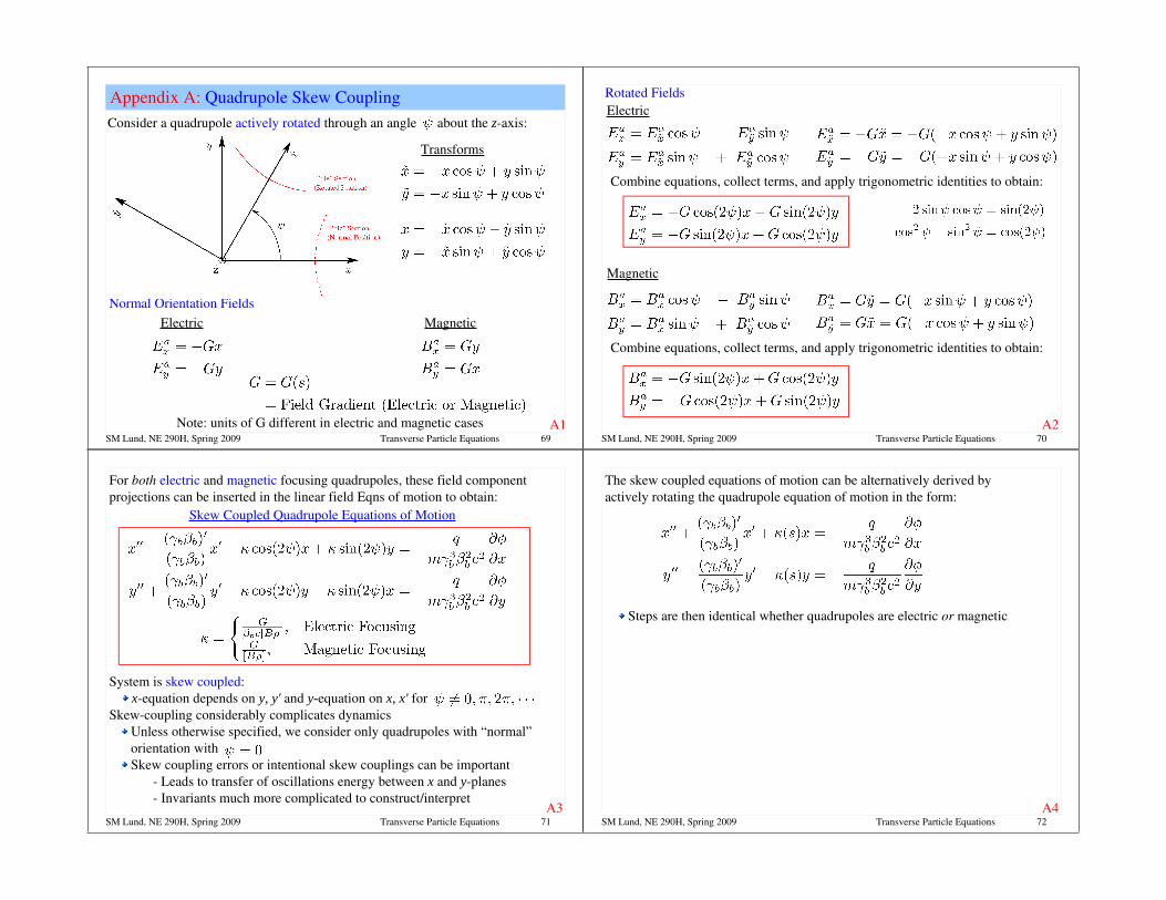
/// Example: Continuous Focusing: Transfer Matrix and Wronskian
///
Principal orbit equations are simple harmonic oscillators with solution:
Transfer matrix gives the familiar solution:
Wronskian invariant is elementary:
SM Lund, NE 290H, Spring 2009 Transverse Particle Equations 110
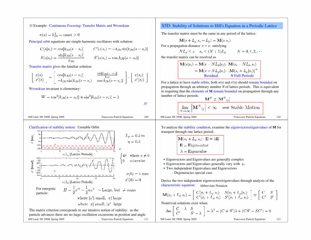
S5D: Stability of Solutions to Hill's Equation in a Periodic Lattice
The transfer matrix must be the same in any period of the lattice:
For a propagation distance satisfying
the transfer matrix can be resolved as
Residual N Full Periods
For a lattice to have stable orbits, both x(s) and x'(s) should remain bounded on propagation through an arbitrary number N of lattice periods. This is equivalent to requiring that the elements of M remain bounded on propagation through any number of lattice periods:
SM Lund, NE 290H, Spring 2009 Transverse Particle Equations 111
Clarification of stability notion: Unstable Orbit
For energetic particle:
The matrix criterion corresponds to our intuitive notion of stability: as the particle advances there are no large oscillation excursions in position and angle.
orbit_stab.png
SM Lund, NE 290H, Spring 2009 Transverse Particle Equations 112
To analyze the stability condition, examine the eigenvectors/eigenvalues of M for transport through one lattice period:
Eigenvectors and Eigenvalues are generally complexEigenvectors and Eigenvalues generally vary with Two independent Eigenvalues and Eigenvectors
Degeneracies special case
Derive the two independent eigenvectors/eigenvalues through analysis of the characteristic equation: Abbreviate Notation
Nontrivial solutions exist when:

SM Lund, NE 290H, Spring 2009 Transverse Particle Equations 113
But we can apply the Wronskian condition:
and we make the notational definition
The characteristic equation then reduces to:
The use of to denote Tr M is in anticipation of later results (see S6) where is identified as the phaseadvance of a stable orbit
There are two solutions to the characteristic equation that we denote
Note that:
SM Lund, NE 290H, Spring 2009 Transverse Particle Equations 114
Consider a vector of initial conditions:
The eigenvectors span twodimensional space. So any initial condition vector can be expanded as:
Then using
Therefore, if is bounded, then the motion is stable. This will always be the case if , corresponding to real with
SM Lund, NE 290H, Spring 2009 Transverse Particle Equations 115
This implies for stability or the orbit that we must have:
In a periodic focusing lattice, this important stability condition places restrictions on the lattice structure (focusing strength) that are generally interpreted in terms of phase advance limits (see: S6).
Accelerator lattices almost always tuned for single particle stability to maintain beam control
Even for intense beams, beam centroid approximately obeys single particle equations of motion when image charges are negligible
Spacecharge and nonlinear applied fields can further limit particle stability Resonances: see: Particle Resonances .... Envelope Instability: see: Transverse Centroid and Envelope .... Higher Order Instability: see: Transverse Kinetic Stability
We will show (see: S6) that for stable orbits can be interpreted as the phaseadvance of single particle oscillations
SM Lund, NE 290H, Spring 2009 Transverse Particle Equations 116
/// Example: Continuous Focusing Stability
///
Principal orbit equations are simple harmonic oscillators with solution:
Stability bound then gives:
Always satisfied for real Confirms known result using formalism: continuous focusing stable
Energy not pumped into or out of particle orbit
The simplest example of the stability criterion applied to periodic lattices will be given in the problem sets: Stability of a periodic thin lens lattice
Analytically find that lattice unstable when focusing kicks sufficiently strong

SM Lund, NE 290H, Spring 2009 Transverse Particle Equations 117
More advanced treatments See: Dragt, Lectures on Nonlinear Orbit Dynamics, AIP Conf Proc 87 (1982)
show that symplectic 2x2 transfer matrices associated with Hill's Equation have only two possible classes of eigenvalue symmetries:
1) Stable 2) Unstable, Lattice Resonance
Occurs for:Occurs in bands when focusing strength is increased beyond
Limited class of possibilities simplifies analysis of focusing lattices
eigen_sym_s.pngeigen_sym_u.png
SM Lund, NE 290H, Spring 2009 Transverse Particle Equations 118
S6: Hill's Equation: Floquet's Theorem and the PhaseAmplitude Form of the Particle Orbit
S6A: Introduction
In this section we consider Hill's Equation:
subject to a periodic applied focusing function
Many results will also hold in more complicated form for a nonperiodic
SM Lund, NE 290H, Spring 2009 Transverse Particle Equations 119
Floquet's Theorem (proof: see standard Mathematics and Mathematical Physics Texts)
The solution to Hill's Equation x(s) has two linearly independent solutions that can be expressed as:
Where w(s) is a periodic function:
Theorem as written only applies for M with nondegenerate eigenvalues. But a similar theorem applies in the degenerate case. A similar theorem is also valid for nonperiodic focusing functions
S6B: Floquet's Theorem
SM Lund, NE 290H, Spring 2009 Transverse Particle Equations 120
S6C: PhaseAmplitude Form of Particle OrbitAs a consequence of Floquet's Theorem, any (stable or unstable) nondegenerate solution to Hill's Equation can be expressed in phaseamplitude form as:
By f
then substitute in Hill's Equation:
Derive equations of motion for by taking derivatives of the phaseamplitude form for x(s):

SM Lund, NE 290H, Spring 2009 Transverse Particle Equations 121
We are free to introduce an additional constraint between A and : Two functions A, to represent one function x allows a constraint
Choose:
Then to satisfy Hill's Equation for all the, coefficient of must also vanish giving:
Eq. (1)
Eq. (2)
SM Lund, NE 290H, Spring 2009 Transverse Particle Equations 122
Eq. (1) Analysis (coefficient of ):
Integrate once:
One commonly rescales the amplitude A(s) in terms of an auxiliary amplitude functions w(s):
such that
This equation can then be integrated to obtain the phasefunction of the particle:
Simplify:Will show laterthat this assumption met for all s
SM Lund, NE 290H, Spring 2009 Transverse Particle Equations 123
With the choice of amplitude rescaling, and Eq. (2) becomes:
Floquet's theorem tells us that we are free to restrict w to be a periodic solution:
Using and :
Eq. (2) Analysis (coefficient of ):
Reduced Expressions for x and x':
SM Lund, NE 290H, Spring 2009 Transverse Particle Equations 124
where w(s) and are amplitude and phasefunctions satisfying:
Initial ( ) amplitudes are constrained by the particle initial conditions as:
or
Amplitude Equations Phase Equations
S6D: Summary: PhaseAmplitude Form of Solution to Hill's Eqn

SM Lund, NE 290H, Spring 2009 Transverse Particle Equations 125
S6E: Points on the PhaseAmplitude Formulation
1) w(s) can be taken as positive definite
/// Proof: Sign choices in w:
///
Let w(s) be positive at some point. Then the equation:
Insures that w can never vanish or change sign. This follows because whenever w becomes small, can become arbitrarily large to turn w before it reaches zero. Thus, to fix phases, we conveniently require that w > 0.
Proof verifies assumption made in analysis that Conversely, one could choose w negative and it would always remain negative for analogous reasons. This choice is not commonly made. Sign choice removes ambiguity in relating initial conditions
to
SM Lund, NE 290H, Spring 2009 Transverse Particle Equations 126
2) w(s) is a unique periodic functionCan be proved using a connection between w and the principal orbit functions
C and S (see: Appendix C and S7)w(s) can be regarded as a special, periodic function describing the lattice
3) The amplitude parameters
depend only on the periodic lattice properties and are independent of the particle initial conditions
4) The phaseadvance
depends on the choice of initial condition . However, the phaseadvance through one lattice period
SM Lund, NE 290H, Spring 2009 Transverse Particle Equations 127
Will be independent of since w is a periodic function with period Will show that (see later in this section)
is the undepressed phase advance of particle oscillations
5) w(s) has dimensions [[w]] = Sqrt[meters]Can prove inconvenient in applications and motivates the use of an alternative “betatron” function
with dimension [[ ]] = meters (see: S7 and S8)
6) On the surface, what we have done: Transform the linear Hill's Equation to a form where a solution to nonlinear axillary equations for w and are needed via the phaseamplitude method seems insane ..... why do it?
Method will help identify the useful CourantSnyder invariant which will aid interpretation of the dynamics (see: S7)Decoupling of initial conditions in the phaseamplitude method will help simplify understanding of bundles of particles in the distribution
SM Lund, NE 290H, Spring 2009 Transverse Particle Equations 128
S6F: Relation between Principal Orbit Functions and PhaseAmplitude Form Orbit Functions
The transfer matrix M of the particle orbit can be expressed in terms of the principal orbit functions C and S as (see: S4):
Use of the phaseamplitude forms and some algebra identifies (see problem sets):

SM Lund, NE 290H, Spring 2009 Transverse Particle Equations 129
/// Aside: Alternatively, it can be shown (see: Appendix C) that w(s) can be related to the principal orbit functions calculated over one Lattice period by:
The formula for in terms of principal orbit functions is useful: (phase advance, see: S6G) is often specified for the lattice and the focusing function is tuned to achieve the specified valueShows that w(s) can be constructed from two principal orbit integrations over one lattice period
Integrations must generally be done numerically for C and S- No root finding required for initial conditions to construct periodic w(s)- can be anywhere in the lattice period and w(s) will be independent
of the specific choice of
SM Lund, NE 290H, Spring 2009 Transverse Particle Equations 130
The form of suggests an underlying CourantSnyder Invariant (see: S7 and Appendix C)
can be applied to calculate max beam particle excursions in the absence of spacecharge effects (see: S8)
Useful in machine design - Exploits CourantSnyder Invariant
///
SM Lund, NE 290H, Spring 2009 Transverse Particle Equations 131
S6G: Undepressed Particle Phase AdvanceWe can now concretely connect for a stable obit to the advance in particle oscillation phase through one lattice period:
From S5D:
Apply the principal orbit representation of M
and use the phaseamplitude identifications of C and S' calculated in S6F:
By periodicity:
SM Lund, NE 290H, Spring 2009 Transverse Particle Equations 132
Applying these results gives:
Thus, is identified as the phase advance of a stable particle orbit through one lattice period:
Again verifies that is independent of since w(s) is periodic with period The stability criterion (see: S5)
is concretely connected to the particle phase advance through one lattice period providing a useful physical interpretation
Consequence:Any periodic lattice with undepressed phase advance satisfying
will have stable single particle orbits.
SM Lund, NE 290H, Spring 2009 Transverse Particle Equations 133
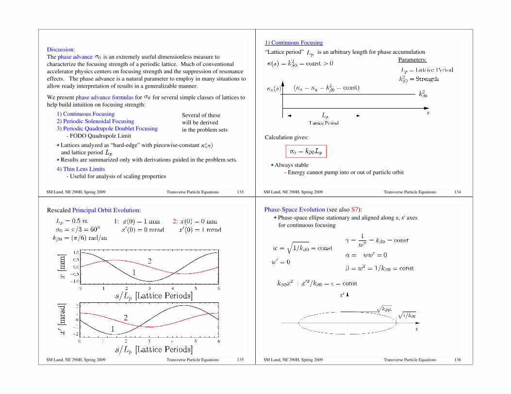
Discussion:The phase advance is an extremely useful dimensionless measure to characterize the focusing strength of a periodic lattice. Much of conventional accelerator physics centers on focusing strength and the suppression of resonance effects. The phase advance is a natural parameter to employ in many situations to allow ready interpretation of results in a generalizable manner.
We present phase advance formulas for for several simple classes of lattices to help build intuition on focusing strength:
1) Continuous Focusing 2) Periodic Solenoidal Focusing3) Periodic Quadrupole Doublet Focusing
FODO Quadrupole Limit
Lattices analyzed as “hardedge” with piecewiseconstant and lattice period Results are summarized only with derivations guided in the problem sets.
4) Thin Lens Limits Useful for analysis of scaling properties
Several of these will be derived in the problem sets
SM Lund, NE 290H, Spring 2009 Transverse Particle Equations 134
1) Continuous Focusing
“Lattice period” is an arbitrary length for phase accumulationParameters:
Calculation gives:
Always stable Energy cannot pump into or out of particle orbit
lat_cont.png
SM Lund, NE 290H, Spring 2009 Transverse Particle Equations 135
Rescaled Principal Orbit Evolution:
1: 2:
ps_cont.png
SM Lund, NE 290H, Spring 2009 Transverse Particle Equations 136
PhaseSpace Evolution (see also S7): Phasespace ellipse stationary and aligned along x, x' axes
for continuous focusing
ps_ellipse_cont.png

SM Lund, NE 290H, Spring 2009 Transverse Particle Equations 137
2) Periodic Solenoidal Focusing
Results are interpreted in the rotating Larmor frame (see S2 and Appendix A)
Parameters:
Characteristics:
Calculation gives:
Can be unstable when becomes large Energy can pump into or out of particle orbit
lat_sol.png
SM Lund, NE 290H, Spring 2009 Transverse Particle Equations 138
Rescaled LarmorFrame Principal Orbit Evolution:
1: 2:
ps_sol.png
Principal orbits in phasespace are identical
SM Lund, NE 290H, Spring 2009 Transverse Particle Equations 139
PhaseSpace Evolution in the Larmor frame (see also: S7): PhaseSpace ellipse rotates and evolves in periodic lattice phasespace properties same as in
Phasespace structure in x-x', y-y' phase space is complicated
ps_sol_cs.png
SM Lund, NE 290H, Spring 2009 Transverse Particle Equations 140
Comments on periodic solenoid results: Larmor frame analysis greatly simplifies results
4D coupled orbit in x-x', y-y' phasespace will be much more intricate in structure
PhaseSpace ellipse rotates and evolves in periodic lattice Periodic structure of lattice changes orbits from simple harmonic

SM Lund, NE 290H, Spring 2009 Transverse Particle Equations 141
3) Periodic Quadrupole Doublet Focusing
Parameters:
Characteristics:
Calculation gives:
Can be unstable when becomes large Energy can pump into or out of particle orbit
SM Lund, NE 290H, Spring 2009 Transverse Particle Equations 142
Comments on Parameters:
The “syncopation” parameter measures how close the Focusing (F) and DeFocusing (D) quadrupoles are to each other in the lattice
The range can be mapped to by simply relabeling quantities. Therefore, we can take:
The special case of a doublet lattice with corresponds to equal drift lengths between the F and D quadrupoles and is called a FODO lattice
Phase advance constraint will be derived for FODO case in problems (algebra much simpler than doublet case)
SM Lund, NE 290H, Spring 2009 Transverse Particle Equations 143
Special Case Doublet Focusing: Periodic Quadrupole FODO LatticeParameters: Characteristics:
Phase advance formula reduces to:
lat_quad_fodo.png
Analysis shows FODO provides stronger focus for same integrated field gradients than doublet due to symmetry
SM Lund, NE 290H, Spring 2009 Transverse Particle Equations 144
Rescaled Principal Orbit Evolution:
1: 2:
ps_quad.png

SM Lund, NE 290H, Spring 2009 Transverse Particle Equations 145
PhaseSpace Evolution (see also: S7): ps_quad_cs.png
SM Lund, NE 290H, Spring 2009 Transverse Particle Equations 146
Comments on periodic FODO quadrupole results: PhaseSpace ellipse rotates and evolves in periodic lattice
Evolution more intricate for Alternating Gradient (AG) focusing than for solenoidal focusing in the Larmor frame Harmonic content of orbits larger for AG focusing than
solenodial focusing Orbit and phase space evolution analogous in y-y' plane
Simply related by an shift in s of the lattice
SM Lund, NE 290H, Spring 2009 Transverse Particle Equations 147
Contrast of Principal Orbits for different focusing: Use previous examples with “equivalent” focusing strength Note that periodic focusing adds harmonic structure
1) Continuous Focusing
2) Periodic Solenoidal Focusing (Larmor Frame)
3) Periodic FODO Quadrupole Doublet Focusing
ps_cont_xc.png
ps_sol_xc.png
ps_quad_xc.png
Simple Harmonic Oscillator
Simple harmonic oscillationsmodified with additional harmonics due to periodic focus
Simple harmonic oscillationsmore strongly modified due to periodic AG focus
SM Lund, NE 290H, Spring 2009 Transverse Particle Equations 148
4) Thin Lens LimitsConvenient to simply understand analytic scaling
Transfer Matrix:
Graphical Interpretation:
thin_lens_interp.png

SM Lund, NE 290H, Spring 2009 Transverse Particle Equations 149
The thin lens limit of “thick” hardedge solenoid and quadrupole focusing lattices presented can be obtained by taking:
Solenoids:
Quadrupoles:
This obtains when applied in the previous formulas:
These formulas can also be derived directly from the drift and thin lens transfer matrices as
Periodic Solenoid
Periodic Quadrupole Doublet
SM Lund, NE 290H, Spring 2009 Transverse Particle Equations 150
Expanded phase advance formulas (thin lens type limit and similar) can be useful in system design studies
Desirable to derive simple formulas relating magnet parameters to Clear analytic scaling trends clarify design tradeoffs
For hard edge periodic lattices, expand formula for to leading order in
/// Example: Periodic Quadrupole Doublet Focusing: Expand previous formula
where:
SM Lund, NE 290H, Spring 2009 Transverse Particle Equations 151
Using these results, plot the Field Gradient and Integrated Gradient for quadrupole doublet focusing needed for per lattice period
///
Gradient ~
Integrated Gradient ~
strength_scale.pngExact (nonexpanded) solutions plotted dashed (almost overlay)Gradient and integrated gradient required depend only weakly on syncopation factor when is near ½ Stronger gradient required for low occupancy but integrated gradient varies little with
SM Lund, NE 290H, Spring 2009 Transverse Particle Equations 152
Appendix C: Calculation of w(s) from Principal Orbit Functions
C1
Evaluate principal orbit expressions of the transfer matrix through one lattice period using
and
to obtain (see principal orbit formulas expressed in phaseamplitude form):

SM Lund, NE 290H, Spring 2009 Transverse Particle Equations 153
Giving:
Or in terms of the betatron formulation (see: S7 and S8) with
Next, calculate w from the principal orbit expression in phaseamplitude form:
C2SM Lund, NE 290H, Spring 2009 Transverse Particle Equations 154
Square and add equations:
Gives:
This result reflects the structure of the underlying CourantSnyder invariant (see: S7)
Use previously identified and write out result:
Formula shows that for a given (used to specify lattice focusing strength), w(s) is given by two linear principal orbits calculated over one lattice period
Easy to apply numericallyC3
SM Lund, NE 290H, Spring 2009 Transverse Particle Equations 155
An alternative way to calculate w(s) is as follows. 1st apply the phaseamplitude formulas for the principal orbit functions with:
Formula requires calculation of at every value of s within lattice periodPrevious formula requires one calculation of
for and any value of
C4SM Lund, NE 290H, Spring 2009 Transverse Particle Equations 156
Matrix algebra can be applied to simplify this result:
Using this result with the previous formula allows the transfer matrix to be calculated only once per period from any initial conditionUsing: Apply Wronskian
condition:
The matrix formula can be shown to the equivalent to the previous one
Methodology applied in: Lund, Chilton, and Lee, PRSTAB 9 064201 (2006) to construct a failsafe iterative matched envelope including spacecharge C5
lat_interval.png

SM Lund, NE 290H, Spring 2009 Transverse Particle Equations 157
S7: Hill's Equation: The CourantSnyder Invariant and Single Particle Emittance
S7A: Introduction
Constants of the motion can simplify the interpretation of dynamics in physicsDesirable to identify constants of motion for Hill's equation for improved understanding of focusing in acceleratorsConstants of the motion are not immediately obvious for Hill's Equation due to svarying focusing forces related to can add and remove energy from the particle
Wronskian symmetry is one useful symmetry Are there other symmetries?
SM Lund, NE 290H, Spring 2009 Transverse Particle Equations 158
/// Illustrative Example: Continuous Focusing/Simple Harmonic Oscillator
Equation of motion:
Constant of motion is the wellknow Hamiltonian/Energy:
///
which shows that the particle moves on an ellipse in xx' phasespace with:Location of particle on ellipse set by initial conditionsAll initial conditions with same energy/H give same ellipse
cf_ps_ellipse.png
SM Lund, NE 290H, Spring 2009 Transverse Particle Equations 159
Question:
For Hill's equation:
does a quadratic invariant exist that can aid interpretation of the dynamics?
Answer we will find:Yes, the CourantSnyder invariant
Comments:Very important in accelerator physics
Helps interpretation of linear dynamics Named in honor of Courant and Synder who popularized it's use in Accelerator physics while codiscovering alternating gradient (AG) focusing in a single seminal (and very elegant) paper:
Courant and Snyder, Theory of the Alternating Gradient Synchrotron, Annals of Physics 3, 1 (1958). Christofolos also understood AG focusing in the same period using a
more heuristic analysis Easily derived using phaseamplitude form of orbit solution
Can be much harder using other methods
SM Lund, NE 290H, Spring 2009 Transverse Particle Equations 160
The phase amplitude method described in S6 makes identification of the invariant elementary. Use the phase amplitude form of the orbit:
where
square and add the equations to obtain the CourantSnyder invariant:
Rearrange the phaseamplitude trajectory equations:
S7B: Derivation of CourantSnyder Invariant

SM Lund, NE 290H, Spring 2009 Transverse Particle Equations 161
Comments on the CourantSnyder Invariant: Simplifies interpretation of dynamics (will show how shortly)Extensively used in accelerator physics Quadratic structure in x-x' defines a rotated ellipse in x-x' phase space. Because
the CourantSnyder invariant can be alternatively expressed as:
Cannot be interpreted as a conserved energy!
The point that the CourantSnyder invariant is not a conserved energy should be elaborated on. The equation of motion:
Is derivable from the Hamiltonian
SM Lund, NE 290H, Spring 2009 Transverse Particle Equations 162
Apply the chainRule with H = H(x,x';s):
Energy of a “kicked” oscillator with is not conserved Energy should not be confused with the CourantSnyder invariant
H is the energy:
Apply the equation of motion:
SM Lund, NE 290H, Spring 2009 Transverse Particle Equations 163
/// Aside: Only for the special case of continuous focusing (i.e., a simple Harmonic oscillator) are the CourantSnyder invariant and energy simply related:
Continuous Focusing:
w equation:
CourantSnyder Invariant:
///SM Lund, NE 290H, Spring 2009 Transverse Particle Equations 164
Interpret the CourantSnyder invariant:
by expanding and isolating terms quadratic terms in x-x' phasespace variables:
The three coefficients in [...] are functions of w and w' only and therefore are functions of the lattice only (not particle initial conditions). They are commonly called “Twiss Parameters” and are expressed denoted as:
Only 2 of the three Twiss parameters are “independent” (i.e., w, w' determine all 3)

SM Lund, NE 290H, Spring 2009 Transverse Particle Equations 165
The area of the invariant ellipse is:Apply standard formulas from Analytic Geometry or calculate
where is the singleparticle emittance:Emittance is the area of the orbit in x-x' phasespace divided by
See problem sets for critical point calculation
cs_ellipse.png
SM Lund, NE 290H, Spring 2009 Transverse Particle Equations 166
/// Aside on Notation: Twiss Parameters and Emittance Units:
///
Emittance Units:x has dimensions of length and x' is a dimensionless angle. So x-x' phasespace area and has dimensions [[ ]] = length. A common choice of units is millimeters (mm) and milliradians (mrad), e.g.,
The definition of the emittance employed is not unique and different workers use a wide variety of symbols. Some common notational choices:
Write the emittance values in units with a , e.g.,
Use caution! Understand conventions being used before applying results!
Twiss Parameters:Use of should not create confusion with kinematic relativistic factors
are absorbed in the focusing function Contextual use of notation unfortunate reality .... not enough symbols!
SM Lund, NE 290H, Spring 2009 Transverse Particle Equations 167
Properties of CourantSnyder Invariant:The ellipse will rotate and change shape as the particle advances through the focusing lattice, but the instantaneous area of the ellipse ( ) remains constant.The location of the particle on the ellipse and the size (area) of the ellipse depends on the initial conditions of the particle.The orientation of the ellipse is independent of the particle initial conditions. All particles move on nested ellipses. Quadratic in the x-x' phasespace coordinates, but is not the transverse particle energy (which is not conserved).
SM Lund, NE 290H, Spring 2009 Transverse Particle Equations 168
The CourantSnyder invariant helps us understand the phasespace evolution of the particles. Knowing how the ellipse transforms (twists and rotates without changing area) is equivalent to knowing the dynamics of a bundle of particles. To see this:General s:
Initial s = :
Apply the components of the transport matrix:
Invert 2x2 matrix and apply det M = 1 (Wronskian):
S7C: Lattice Maps

SM Lund, NE 290H, Spring 2009 Transverse Particle Equations 169
Insert expansion for in the initial ellipse expression, collect factors of x^2, xx', and x'^2, and equate to general s ellipse expression:
Collect coefficients of x^2, xx', and x'^2 and summarize in matrix form:
This result can be applied to illustrate how a bundle of particles will evolve from an initial location in the lattice subject to the linear focusing optics in the machine using only principal orbits C, S, C', and S'
Principal orbits will generally need to be calculated numerically Intuition can be built up using simple analytical results (hard edge etc)
SM Lund, NE 290H, Spring 2009 Transverse Particle Equations 170
/// Example: Ellipse Evolution in a simple kicked focusing lattice
///
Drift:
Thin Lens:focal length f
For further examples of phasespace ellipse evolutions in standard lattices, see: S6G
lat_maps.png
SM Lund, NE 290H, Spring 2009 Transverse Particle Equations 171
S8: Hill's Equation: The Betatron Formulation of the Particle Orbit and Maximum Orbit Excursions S8A: Formulation
The phaseamplitude form of the particle orbit analyzed in S6 of
is not a unique choice. Here, w has dimensions (meters)^(1/2), which can render it inconvenient in applications. Due to this and the utility of the Twiss parameters used in describing orientation of the phasespace ellipse associated with the CourantSnyder invariant (see: S7) on which the particle moves, it is convenient to define an alternative, Betatron representation of the orbit with:
Betatron function:
Emittance:
Phase:
The betatron function has dimensions [[ ]] = metersSM Lund, NE 290H, Spring 2009 Transverse Particle Equations 172
Comments:Use of the symbol for the betatron function does not result in confusion with relativistic factors such as since the context of use will make clear
Relativistic factors often absorbed in lattice focusing function and do not directly appear in the dynamical descriptions
The initial phase will differer in the w and betatron phaseamplitude forms in order to match initial conditions in x and x' at
We do not distinguish for reasons of notational simplicity The change in phase is the same for both formulations:
Add material on initial condition correspondence in future editions of notes

SM Lund, NE 290H, Spring 2009 Transverse Particle Equations 173
From the equation for w:
the betatron function is described by:
The betatron function can, analogously to the wfunction, as a special function defined by the periodic latticeAgain, the equation is nonlinear and must generally be solved numerically
SM Lund, NE 290H, Spring 2009 Transverse Particle Equations 174
From the orbit equation
the maximum and minimum possible particle excursions occur where:
Thus, the max radial extent of all particle oscillations in the beam distribution occurs for the particle with the max single particle emittance since the particles move on nested ellipses:
Assumes sufficient numbers of particles to populate all possible phases corresponds to the min possible machine aperture to prevent particle losses
Practical aperture choice influenced by: resonance effects due to nonlinear applied fields, spacecharge, scattering, finite particle lifetime, ....
S8B: Maximum Orbit Excursions
SM Lund, NE 290H, Spring 2009 Transverse Particle Equations 175
From:
Comments:Equation is analogous to the statistical envelope equation derived by J.J. Barnard in the Intro Lectures when a spacecharge term is added and the max single particle emittance is interpreted as a statistical emittance
correspondence will become more concrete in later lecturesThis correspondence will be developed more extensively in later lectures on Transverse Centroid and Envelope Descriptions of Beam Evolution and
Transverse Equilibrium Distributions
We immediately obtain an equation for the maximum locus (envelope) of radial particle excursions as:
SM Lund, NE 290H, Spring 2009 Transverse Particle Equations 176
S9: Momentum Spread Effects and BendingS9A: FormulationExcept for brief digressions in S1 and S4, we have concentrated on particle dynamics where all particles have the design longitudinal momentum:
Realistically, there will always be a finite spread of particle momentum within a beam slice, so we take:
Typical values of momentum spread in a beam with a single species of particles with conventional sources and accelerating structures:
The spread of particle momentum can modify particle orbits, particularly when dipole bends are present since the bend radius depends strongly on the particle momentum

SM Lund, NE 290H, Spring 2009 Transverse Particle Equations 177
To better understand this effect, we analyze the particle equations of motion with leadingorder momentum spread (see: S1) effects retained:
Neglects:Spacecharge: Nonlinear applied focusing: contain only linear focus termsAcceleration:
Magnetic Dipole Bend
SM Lund, NE 290H, Spring 2009 Transverse Particle Equations 178
In the equations of motion, it is important to understand that of the magnetic bends are set from the radius R required by the design particle orbit (see: S1 for details)
Equations must be modified slightly for electric bends (see S1) y-plane bends also require modification
The focusing strengths are defined with respect to the design momentum:
Terms in the equations of motion associated with momentum spread ( ) can be lumped into two classes:
1) Chromatic Associated with Focusing2) Dispersive Associated with Dipole Bends
SM Lund, NE 290H, Spring 2009 Transverse Particle Equations 179
Present in both x- and y-equations of motion and result from applied focusing strength changing with deviations in momentum:
Generally of lesser importance (smaller corrections) relative to dispersive terms (S9C) except where the beam is focused onto a target (small spot) or when momentum spreads are largeLectures by J.J. Barnard on Heavy Ion Fusion and Final Focusing will overview consequences of chromatic effects in final focus optics
S9B: Chromatic Effects
to neglect bending terms
SM Lund, NE 290H, Spring 2009 Transverse Particle Equations 180
Present in only the x-equation of motion and result from bending. Neglecting chromatic terms:
Particles are bent at different radii when the momentum deviates from the design value ( ) leading to changes in the particle orbit
Dispersive terms contain the bend radius R
Generally, the bend radii R are large and is small, and we can take to leading order:
Term 2:
Term 1:
S9C: Dispersive Effects
Term 1 Term 2

SM Lund, NE 290H, Spring 2009 Transverse Particle Equations 181
The equations of motion then become:
Generally, the x-equation is solved for periodic lattices by exploiting the linear structure of the equation and linearly resolving:
The yequation is not changed from the usual Hill's Equation
where is the general solution to the Hill's Equation:
and is the periodic solution to:
SM Lund, NE 290H, Spring 2009 Transverse Particle Equations 182
This convenient resolution of the orbit x(s) can always be made because the homogeneous solution will be adjusted to match any initial condition
Note that provides a measure of the offset of the particle orbit relative to the design orbit resulting from a small deviation of momentum ( )
x(s) = 0 defines the design orbit
dplt.png
/// Example: Simple piecewise constant focusing and bending lattice
///
SM Lund, NE 290H, Spring 2009 Transverse Particle Equations 183
Uniform Bundle of particles D = 0 Same Bundle of particles D 0 Gaussian distribution of momentum
spread distorts the x-y distribution extents in x but not in y
/// Example: Dispersion broadens the xdistribution
disp_stat_nom.png disp_stat_pert.png///
D=0 extent
SM Lund, NE 290H, Spring 2009 Transverse Particle Equations 184
ring.png
Many rings are designed to focus the dispersion function D(s) to small values in straight sections even though the lattice has strong bends
Desirable since it allows smaller beam sizes at locations near where D = 0 and these locations can be used to insert and extract (kick) the beam into and out of the ring with minimal losses
Since average value of D is dictated by ring size and focusing strength (see example next page) this variation in values can lead to D being
larger in other parts of the ring Quadrupole triplet focusing lattices are often employed in rings since the optics allows sufficient flexibility to tune D while simultaneously allowing particle phase advances to also be adjusted
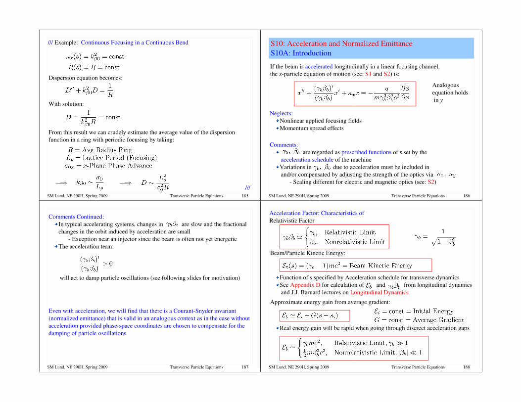
SM Lund, NE 290H, Spring 2009 Transverse Particle Equations 185
/// Example: Continuous Focusing in a Continuous Bend
///
Dispersion equation becomes:
With solution:
From this result we can crudely estimate the average value of the dispersion function in a ring with periodic focusing by taking:
SM Lund, NE 290H, Spring 2009 Transverse Particle Equations 186
S10: Acceleration and Normalized EmittanceS10A: Introduction
If the beam is accelerated longitudinally in a linear focusing channel, the xparticle equation of motion (see: S1 and S2) is:
Neglects:Nonlinear applied focusing fields Momentum spread effects
Comments: are regarded as prescribed functions of s set by the
acceleration schedule of the machineVariations in due to acceleration must be included in
and/or compensated by adjusting the strength of the optics via Scaling different for electric and magnetic optics (see: S2)
Analogous equation holds in y
SM Lund, NE 290H, Spring 2009 Transverse Particle Equations 187
Comments Continued:In typical accelerating systems, changes in are slow and the fractional changes in the orbit induced by acceleration are small
Exception near an injector since the beam is often not yet energeticThe acceleration term:
Even with acceleration, we will find that there is a CourantSnyder invariant (normalized emittance) that is valid in an analogous context as in the case without acceleration provided phasespace coordinates are chosen to compensate for the damping of particle oscillations
will act to damp particle oscillations (see following slides for motivation)
SM Lund, NE 290H, Spring 2009 Transverse Particle Equations 188
Acceleration Factor: Characteristics of Relativistic Factor
Beam/Particle Kinetic Energy:
Function of s specified by Acceleration schedule for transverse dynamicsSee Appendix D for calculation of and from longitudinal dynamics
and J.J. Barnard lectures on Longitudinal Dynamics
Approximate energy gain from average gradient:
Real energy gain will be rapid when going through discreet acceleration gaps

SM Lund, NE 290H, Spring 2009 Transverse Particle Equations 189
Identify relativistic factor with average gradient energy gain:
Relativistic Limit:
Nonrelativistic Limit:
Expect Relativistic and Nonrelativistic motion to have similar solutions Parameters for each case will often be quite different
SM Lund, NE 290H, Spring 2009 Transverse Particle Equations 190
/// Aside: Acceleration and Continuous Focusing Orbits with Assume relativistic motion and negligible spacecharge:
Then the equation of motion reduces to:
This equation is the equation of a Bessel Function of order zero:
SM Lund, NE 290H, Spring 2009 Transverse Particle Equations 191
Solving for the constants in terms of the particle initial conditions:
Invert matrix to solve for constants in terms of initial conditions:
Comments:Bessel functions behave like damped harmonic oscillators
See any texts on Mathematical Physics or Applied MathematicsNonrelativistic limit solution is not described by a Bessel Function solution
Properties of solution will be similar though (similar special function) The coefficient in the damping term has a factor of 2 difference, preventing exact Bessel function form
SM Lund, NE 290H, Spring 2009 Transverse Particle Equations 192
///
Using this solution, plot the orbit for (contrived parameters for illustration only):
Solution shows damping: phase volume scaling
accel.png

SM Lund, NE 290H, Spring 2009 Transverse Particle Equations 193
“Guess” transformation to apply motivated by conjugate variable arguments (see: J.J. Barnard, Intro. Lectures)
Then:
The inverse phasespace transforms will also be useful later:
S10B: Transformation to Normal Form
SM Lund, NE 290H, Spring 2009 Transverse Particle Equations 194
Applying these results, the particle x equation of motion with acceleration becomes:
Note:Factor of difference from untransformed expression in the spacecharge coupling coefficient
It is instructive to also transform the Possion equation associated with the spacecharge term:
Transform:
SM Lund, NE 290H, Spring 2009 Transverse Particle Equations 195
Using these results, Poisson's equation becomes:
Or defining a transformed potential
Applying these results, the xequation of motion with acceleration becomes:
Usual form of the spacecharge coefficient with rather than is restored when expressed in terms of the transformed potential
SM Lund, NE 290H, Spring 2009 Transverse Particle Equations 196
An additional step can be taken to further stress the correspondence between the transformed system with acceleration and the untransformed system in the absence of acceleration. Denote an effective focusing strength:
incorporates acceleration terms beyond factors already included in the definition of (see: S2):
The transformed equation of motion with acceleration then becomes:

SM Lund, NE 290H, Spring 2009 Transverse Particle Equations 197
The transformed equation with acceleration has the same form as the equation in the absence of acceleration. If spacecharge is negligible ( ) we have:
Accelerating System NonAccelerating System
Therefore, all previous analysis on phaseamplitude methods and CourantSnyder invariants associated with Hill's equation in x-x' phasespace can be immediately applied to phasespace for an accelerating beam
Focusing field strengths need to be adjusted to maintain periodicity of in the presence of acceleration
Not possible to do exactly, but can be approximate for weak accelerationSM Lund, NE 290H, Spring 2009 Transverse Particle Equations 198
S10C: Phase Space Relation Between Transformed and UnTransformed Systems
It is instructive to relate the transformed phasespace area in tilde variables to the usual x-x' phase area:
where J is the Jacobian:
Thus:
Inverse transformsderived previously:
SM Lund, NE 290H, Spring 2009 Transverse Particle Equations 199
Factor compensates for acceleration induced damping in particle orbits Normalized emittance is very important in design of lattices to transport accelerating beams
Designs usually made assuming conservation of normalized emittanceSame result that J.J. Barnard motivated in the Intro. Lectures using alternative methods
Based on this area transform, if we define the (instantaneous) phase space area of the orbit trance in x-x' to be “regular emittance”, then this emittance is related to the “normalized emittance” in phasespace by:
SM Lund, NE 290H, Spring 2009 Transverse Particle Equations 200
Appendix D: Accelerating Fields and Calculation of Changes in gamma*beta
The transverse particle equation of motion with acceleration was derived in a Cartesian system by approximating (see: S1):
using
to obtain:
D1

SM Lund, NE 290H, Spring 2009 Transverse Particle Equations 201
Changes in are calculated from the longitudinal particle equation of motion:
Term 1 Term 2 Term 3
Using steps similar to those in S1, we approximate terms:
Term 1:
Term 2:
Term 3:
is a quasistatic approximation accelerating potential (see next pages)
Transverse magnetic fields typically only weakly change particle energy and terms can be neglected relative to others D2
SM Lund, NE 290H, Spring 2009 Transverse Particle Equations 202
The longitudinal particle equation of motion for then reduces to:
Some algebra then shows that:
Giving:
Which can then be integrated to obtain:
D3
SM Lund, NE 290H, Spring 2009 Transverse Particle Equations 203
We denote the onaxis accelerating potential as:
Can represent RF or induction accelerating gap fields See: J.J. Barnard lectures for more details
Giving:
These equations can be solved for the consistent variation of in the transverse equations of motion:
D4SM Lund, NE 290H, Spring 2009 Transverse Particle Equations 204
In the nonrelativistic limit:
Giving the familiar result of a nonrelativistic particle gaining energy when falling down a potential gradient:
Using this result, in the nonrelativistic limit we can take in the transverse particle equation of motion:
Nonrelativistic limit results
D5

SM Lund, NE 290H, Spring 2009 Transverse Particle Equations 205
Quasistatic potential expansionIn the quasistatic approximation, the accelerating potential can be expanded in the axisymmetric limit as:
See: J.J. Barnard, Intro Lectures; and Reiser, Theory and Design of Charged Particle Beams, (1994, 2008) Sec. 3.3.
The longitudinal acceleration also result in a transverse focusing field
Results can be used to cast acceleration terms in more convenient forms. See J.J. Barnard lectures for more details. D6
SM Lund, NE 290H, Spring 2009 Transverse Particle Equations 206
These notes will be corrected and expanded for reference and future editions of US Particle Accelerator School and University of California at Berkeley courses:
“Beam Physics with Intense Space Charge”“Interaction of Intense Charged Particle Beams with Electric and Magnetic Fields”
by J.J. Barnard and S.M. Lund
Corrections and suggestions for improvements are welcome. Contact:
Steven M. Lund Lawrence Berkeley National Laboratory BLDG 47 R 01121 Cyclotron Road Berkeley, CA 947208201
[email protected](510) 486 – 6936
Please do not remove author credits in any redistributions of class material.
SM Lund, NE 290H, Spring 2009 Transverse Particle Equations 207
References: For more information see:
Earlier versions of course notes posted online (present will also be posted with corrections):J. Barnard and S. Lund, Intense Beam Physics, US Particle Accelerator School Notes, http://uspas.fnal.gov/lect_note.html (2006, 2004)Basic introduction on many of the topics covered:M. Reiser, Theory and Design of Charged Particle Beams, Wiley (1994, revised 2008)Review by author (with similar perspective to notes) with material on phase advances, lattice focusing strength, etc. S.M. Lund and B. Bukh, Stability Properties of the Transverse Envelope Equations Describing Intense Ion Beam Transport, Phys. Rev. Special Topics – Accelerators and Beams (2004). Hill's Equation, Floquet's theorem, CourantSnyder invariants, and dispersion functions: H. Wiedermann, Particle Accelerator Physics, SpringerVerlag (1995)
SM Lund, NE 290H, Spring 2009 Transverse Particle Equations 208
Particle equations of motion with bends and momentum spread:D.A. Edwards and M.J. Syphers, An Introduction to the Physics of High Energy Accelerators, Wiley (1993). Original, classic paper on strong focusing and CourantSnyder invariants applied to accelerator physics. Remains one of the best formulated treatments to date:E.D. Courant and H. S. Snyder, Theory of the Alternating Gradient Synchrotron, Annals Physics 3, 1 (1958). More mathematical treatment of transfer matrices and stabilityA. Dragt, Lectures on Nonlinear Orbit Dynamics, in “Physics of High Energy Accelerators,” edited by R.A. Carrigan, F.R. Hudson, and M. Month (AIP Conf. Proc. No. 87, New York, 1982), p. 147. Phaseamplitude methods, Larmor frame: J.D. Lawson, The Physics of Charged Particle Beams, Oxford University Priess (1977). Solenoidal focusing and the Larmor frame:H. Wiedemann, Particle Accelerator Physics II: Nonlinear and Higher Order Beam Dynamics, Springer (1995).

SM Lund, NE 290H, Spring 2009 Transverse Particle Equations 209
Acknowledgments:
Klaus Halbach educated one of the authors (S.M. Lund) on the use of complex variable theory to simplify analysis of multipole fields employed in S3: Description of Applied Focusing Fields.
Considerable help was provided by Guliano Franchetti (GSI) in educating one of the authors (S.M. Lund) in phaseamplitude methods described in this lecture.
Edward P. Lee (LBNL) helped formulate parts of material presented in S10: Acceleration and Normalized Emittance.