
TransPose: Real-time 3D Human Translation and Pose ...
13
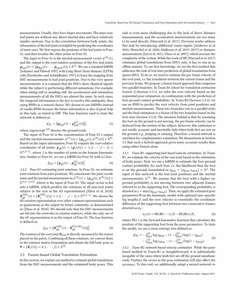
TransPose: Real-time 3D Human Translation and Pose Estimation with Six Inertial Sensors XINYU YI, BNRist and school of soſtware, Tsinghua University, China YUXIAO ZHOU, BNRist and school of soſtware, Tsinghua University, China FENG XU, BNRist and school of soſtware, Tsinghua University, China Fig. 1. We present a real-time motion capture approach that estimates poses and global translations using only six inertial measurement units. As a purely inertial sensor-based approach, our system does not suffer from occlusion, challenging environment or multi-person ambiguities, and achieves long-range capture with real-time performance. Motion capture is facing some new possibilities brought by the inertial sensing technologies which do not suffer from occlusion or wide-range recordings as vision-based solutions do. However, as the recorded signals are sparse and quite noisy, online performance and global translation estimation turn out to be two key difficulties. In this paper, we present TransPose, a DNN- based approach to perform full motion capture (with both global translations and body poses) from only 6 Inertial Measurement Units (IMUs) at over 90 fps. For body pose estimation, we propose a multi-stage network that estimates leaf-to-full joint positions as intermediate results. This design makes the pose estimation much easier, and thus achieves both better accuracy and lower computation cost. For global translation estimation, we propose a supporting- foot-based method and an RNN-based method to robustly solve for the global translations with a confidence-based fusion technique. Quantitative and qualitative comparisons show that our method outperforms the state-of- the-art learning- and optimization-based methods with a large margin in Authors’ addresses: Xinyu Yi, BNRist and school of software, Tsinghua University, Beijing, China, [email protected]; Yuxiao Zhou, BNRist and school of software, Tsinghua University, Beijing, China, [email protected]; Feng Xu, BNRist and school of software, Tsinghua University, Beijing, China, xufeng2003@gmail. com. Permission to make digital or hard copies of all or part of this work for personal or classroom use is granted without fee provided that copies are not made or distributed for profit or commercial advantage and that copies bear this notice and the full citation on the first page. Copyrights for components of this work owned by others than the author(s) must be honored. Abstracting with credit is permitted. To copy otherwise, or republish, to post on servers or to redistribute to lists, requires prior specific permission and/or a fee. Request permissions from [email protected]. © 2021 Copyright held by the owner/author(s). Publication rights licensed to ACM. 0730-0301/2021/8-ART86 $15.00 https://doi.org/10.1145/3450626.3459786 both accuracy and efficiency. As a purely inertial sensor-based approach, our method is not limited by environmental settings (e.g., fixed cameras), making the capture free from common difficulties such as wide-range motion space and strong occlusion. CCS Concepts: • Computing methodologies → Motion capture. Additional Key Words and Phrases: IMU, Pose Estimation, Inverse Kinemat- ics, Real-time, RNN ACM Reference Format: Xinyu Yi, Yuxiao Zhou, and Feng Xu. 2021. TransPose: Real-time 3D Human Translation and Pose Estimation with Six Inertial Sensors. ACM Trans. Graph. 40, 4, Article 86 (August 2021), 13 pages. https://doi.org/10.1145/3450626. 3459786 1 INTRODUCTION Human motion capture (mocap), aiming at reconstructing 3D human body movements, plays an important role in various applications such as gaming, sports, medicine, VR/AR, and movie production. So far, vision-based mocap solutions take the majority in this topic. One category requires attaching optical markers on human bodies and leverages multiple cameras to track the markers for motion cap- ture. The marker-based systems such as Vicon 1 are widely applied and considered accurate enough for industrial usages. However, such approaches require expensive infrastructures and intrusive devices, which make them undesirable for consumer-level usages. 1 https://www.vicon.com/ ACM Trans. Graph., Vol. 40, No. 4, Article 86. Publication date: August 2021.
Transcript of TransPose: Real-time 3D Human Translation and Pose ...
TransPose: Real-time 3D Human Translation and Pose Estimation withSix Inertial Sensors
XINYU YI, BNRist and school of software, Tsinghua University, ChinaYUXIAO ZHOU, BNRist and school of software, Tsinghua University, ChinaFENG XU, BNRist and school of software, Tsinghua University, China
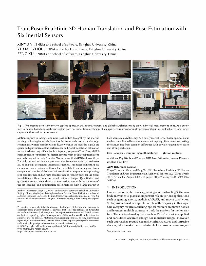
Fig. 1. We present a real-time motion capture approach that estimates poses and global translations using only six inertial measurement units. As a purelyinertial sensor-based approach, our system does not suffer from occlusion, challenging environment or multi-person ambiguities, and achieves long-rangecapture with real-time performance.
Motion capture is facing some new possibilities brought by the inertialsensing technologies which do not suffer from occlusion or wide-rangerecordings as vision-based solutions do. However, as the recorded signals aresparse and quite noisy, online performance and global translation estimationturn out to be two key difficulties. In this paper, we present TransPose, a DNN-based approach to perform full motion capture (with both global translationsand body poses) from only 6 Inertial Measurement Units (IMUs) at over 90 fps.For body pose estimation, we propose a multi-stage network that estimatesleaf-to-full joint positions as intermediate results. This designmakes the poseestimation much easier, and thus achieves both better accuracy and lowercomputation cost. For global translation estimation, we propose a supporting-foot-based method and an RNN-based method to robustly solve for the globaltranslations with a confidence-based fusion technique. Quantitative andqualitative comparisons show that our method outperforms the state-of-the-art learning- and optimization-based methods with a large margin in
Authors’ addresses: Xinyu Yi, BNRist and school of software, Tsinghua University,Beijing, China, [email protected]; Yuxiao Zhou, BNRist and school ofsoftware, Tsinghua University, Beijing, China, [email protected]; Feng Xu,BNRist and school of software, Tsinghua University, Beijing, China, [email protected].
Permission to make digital or hard copies of all or part of this work for personal orclassroom use is granted without fee provided that copies are not made or distributedfor profit or commercial advantage and that copies bear this notice and the full citationon the first page. Copyrights for components of this work owned by others than theauthor(s) must be honored. Abstracting with credit is permitted. To copy otherwise, orrepublish, to post on servers or to redistribute to lists, requires prior specific permissionand/or a fee. Request permissions from [email protected].© 2021 Copyright held by the owner/author(s). Publication rights licensed to ACM.0730-0301/2021/8-ART86 $15.00https://doi.org/10.1145/3450626.3459786
both accuracy and efficiency. As a purely inertial sensor-based approach, ourmethod is not limited by environmental settings (e.g., fixed cameras), makingthe capture free from common difficulties such as wide-range motion spaceand strong occlusion.
CCS Concepts: • Computing methodologies→ Motion capture.
Additional Key Words and Phrases: IMU, Pose Estimation, Inverse Kinemat-ics, Real-time, RNN
ACM Reference Format:Xinyu Yi, Yuxiao Zhou, and Feng Xu. 2021. TransPose: Real-time 3D HumanTranslation and Pose Estimation with Six Inertial Sensors.ACM Trans. Graph.40, 4, Article 86 (August 2021), 13 pages. https://doi.org/10.1145/3450626.3459786
1 INTRODUCTIONHumanmotion capture (mocap), aiming at reconstructing 3D humanbody movements, plays an important role in various applicationssuch as gaming, sports, medicine, VR/AR, and movie production.So far, vision-based mocap solutions take the majority in this topic.One category requires attaching optical markers on human bodiesand leverages multiple cameras to track the markers for motion cap-ture. The marker-based systems such as Vicon1 are widely appliedand considered accurate enough for industrial usages. However,such approaches require expensive infrastructures and intrusivedevices, which make them undesirable for consumer-level usages.
1https://www.vicon.com/
ACM Trans. Graph., Vol. 40, No. 4, Article 86. Publication date: August 2021.
86:2 • Xinyu Yi, Yuxiao Zhou, and Feng Xu
Recently, another category focuses on pose estimation using a fewRGB or RGB-D cameras [Chen et al. 2020; Habibie et al. 2019; Mehtaet al. 2020; Tome et al. 2018; Trumble et al. 2016; Xiang et al. 2019].Although these methods are much more lightweight, they are sen-sitive to the appearance of humans since distinguishable featuresneed to be extracted from images. In consequence, these methodsusually work poorly for textureless clothes or challenging environ-ment lighting. Furthermore, all vision-based approaches suffer fromocclusion. Such a problem can sometimes be solved by setting densecameras (which further makes the system heavy and expensive), butit is often impractical in some applications. For example, it is verydifficult to arrange cameras in a common room full of furniture orobjects, which may occlude the subject from any direction. Anotherlimitation of vision-based approaches is that the performers areusually restricted in a fixed space volume. For daily activities suchas large-range walking and running, carefully controlled movingcameras are required to record enough motion information, whichis very hard to achieve [Xu et al. 2016]. These disadvantages arefatal flaws for many applications and thus lead to limited usabilityof the vision-based solutions.In contrast to vision-based systems, motion capture using body-
worn sensors is environment-independent and occlusion-unaware.It does not require complicated facility setups and lays no constrainton the range of movements. Such characteristics make it more suit-able for customer-level usages. As a result, motion capture usinginertial sensors is gaining more and more focus in recent years. Mostrelated works leverage Inertial Measurement Units (IMUs) to recordmotion inertia, which are economical, lightweight, reliable, and com-monly used in a fast-growing number of wearables such as watches,wristbands, and glasses. The commercial inertial mocap system,Xsens2, uses 17 IMUs to estimate joint rotations. Although accurate,the dense placement of IMUs is inconvenient and intrusive, prevent-ing performers from moving freely. On the other hand, the facilityrequirements for such a system are still beyond the acceptance ofnormal customers. The work of SIP [Marcard et al. 2017] demon-strates that it is feasible to reconstruct human motions from only 6IMUs. However, as an optimization-based method, it needs to accessthe entire sequence and takes a long time to process. The followingstate-of-the-art work, DIP [Huang et al. 2018], achieves real-timeperformance with better quality by leveraging a bidirectional RNN,also using 6 IMUs. However, it still fails on challenging poses, andthe frame rate of 30 fps is not sufficient to capture fast movements,which are very common in practical applications. More importantly,it only estimates body poses without global movements which arealso important in many applications such as VR and AR. The IMUitself is incapable of measuring distances directly. Some previousworks [Liu et al. 2011; Vlasic et al. 2007] use additional ultrasonicsensors to measure global translations, which are expensive andsubject to occlusion. Other possible solutions use GPS localization,which is not accurate enough and only works in outdoor capture. Asa result, super-real-time estimation of both body poses and globaltranslations from sparse worn sensors is still an open problem.To this end, we introduce our approach, TransPose, which es-
timates global translations and body poses from only 6 IMUs at
2https://www.xsens.com/
unprecedented 90 fps with state-of-the-art accuracy. Performingmotion capture from sparse IMUs is extremely challenging, as theproblem is severely under-constrained. We propose to formulate thepose estimation task in a multi-stage manner including 3 subtasks,each of which is easier to solve, and then estimate the global transla-tions using the fusion of two different but complementary methods.As a result, our whole pipeline achieves lower errors but better run-time performance. Specifically, for multi-stage pose estimation, thetask of each stage is listed as follows: 1) leaf joint position estimationestimates the positions of 5 leaf joints from the IMU measurements;2) joint position completion regresses the positions of all 23 jointsfrom the leaf joints and the IMU signals; 3) inverse kinematics solversolves for the joint rotations from positions, i.e. the inverse kine-matics (IK) problem. For fusion-based global translation estimation,we combine the following two methods: 1) foot-ground contact es-timation estimates the foot-ground contact probabilities for bothfeet from the leaf joint positions and the IMU measurements, andcalculates the root translations on the assumption that the foot witha larger contact probability is not moving; 2) root velocity regressorregresses the local velocities of the root in its own coordinate framefrom all joint positions and the IMU signals.
The design of using separate steps in the pose estimation is basedon our observation that estimating joint positions as an intermedi-ate representation is easier than regressing the rotations directly.We attribute this to the nonlinearity of the rotation representation,compared with the positional formulation. On the other hand, per-forming IK tasks with neural networks has already been well inves-tigated by previous works [Holden 2018; Zhou et al. 2018, 2020a,b].However, these works neglect the importance of motion history. Asthe IK problem is ill-posed, the motion ambiguity is commonly seen,which can only be eliminated according to motion history. Here, ineach stage, we incorporate a bidirectional recurrent neural network(biRNN) [Schuster and Paliwal 1997] to maintain motion history.This is similar to [Huang et al. 2018], but due to our 3-stage design,our network is significantly smaller with higher accuracy.
As for the global translation estimation, the intuition behind is topredict which foot contacts the ground and fix the contacting footto deduce the root movement from the estimated pose. Besides, tocope with the cases where no foot is on the ground, we further usean RNN to regress the root translation as a complement. Finally, ourmethod merges these two estimations to predict the final translationusing the fusion weight determined by the foot-ground contactprobability. The inspiration comes from [Shimada et al. 2020; Zouet al. 2020] which leverage foot-ground contact constraints to reducefoot-sliding artifacts in vision-based mocap, but we have a differentpurpose which is to solve for the translation from the estimatedpose. As shown in the experiments, this method can handle mostmovements like walking, running, and challenging jumping.We evaluate our approach on public datasets, where we out-
perform the previous works DIP and SIP by a large margin bothqualitatively and quantitatively with various metrics, including po-sitional and rotational error, temporal smoothness, runtime, etc.We also present live demos that capture a variety of challengingmotions where the performer can act freely regardless of occlusionor range. These experiments demonstrate our significant superiorityto previous works. In conclusion, our contributions are:
ACM Trans. Graph., Vol. 40, No. 4, Article 86. Publication date: August 2021.
TransPose: Real-time 3D Human Translation and Pose Estimation with Six Inertial Sensors • 86:3
• A very fast and accurate approach for real-time motion cap-ture with global translation estimation using only 6 IMUs.
• A novel structure to perform pose estimation which explicitlyestimates joint positions as intermediate subtasks, resultingin higher accuracy and less runtime.
• The first method to explicitly estimate global translations inreal-time from as sparse as 6 IMUs only.
2 RELATED WORKThe research on humanmotion capture has a long history, especiallyfor the vision-based motion capture. Since this is not the category ofthis work, we refer readers to the surveys [Moeslund and Granum2001; Moeslund et al. 2006] for more information. In this section,we mainly review the works using inertial sensors (or combinedwith other sensors) which are closely related to our approach.
2.1 Combining IMUs with Other Sensors or CamerasTypically, a 9-axis IMU contains 3 components: an accelerometerthat measures accelerations, a gyroscope that measures angularvelocities, and a magnetometer that measures directions. Based onthese direct measurements, the drift-free IMU orientations can besolved [Bachmann et al. 2002; Del Rosario et al. 2018; Foxlin 1996;Roetenberg et al. 2005; Vitali et al. 2020] leveraging Kalman filter orcomplementary filter algorithms. However, reconstructing humanposes from a sparse set of IMUs is an under-constrained problem, asthe sensors can only provide orientation and acceleration measure-ments which are insufficient for accurate pose estimation. To copewith this difficulty, one category of works [Liu et al. 2011; Vlasicet al. 2007] propose to utilize additional ultrasonic distance sensorsto reduce the drift in joint positions. In the work of [Liu et al. 2011],database searching is used for similar sensor measurements, and theresults help to construct a local linear model to regress the currentpose online. Although the global position can be determined byleveraging the distance sensors, subjects can only act within a fixedvolume to keep that the distance can be measured by ultrasonicsensors. Another category of works propose to combine IMUs withvideos [Gilbert et al. 2018; Henschel et al. 2020; Malleson et al. 2019,2017; Marcard et al. 2016; Pons-Moll et al. 2011, 2010; Zhang et al.2020], RGB-D cameras [Helten et al. 2013; Zheng et al. 2018], oroptical markers [Andrews et al. 2016]. Gilbert et al. [Gilbert et al.2018] fuse multi-viewpoint videos with IMU signals and estimatehuman poses using 3D convolutional neural networks and recur-rent neural networks. Global positions can also be determined insome works [Andrews et al. 2016; Malleson et al. 2019, 2017] dueto the additional information from vision. Although these worksachieve great accuracy, due to the need of vision, the capture suffersfrom occlusion and challenging lighting conditions, and can onlybe performed within a restricted area to keep the subject inside thecamera field of view. To this end, Marcard et al. [von Marcard et al.2018] propose to use a moving camera to break the limitation onthe space volume. Nonetheless, all the methods that require visualor distance sensor inputs are substantially limited by the captureenvironment and occlusion.
2.2 Methods Based on Pure Inertial SensorsAs opposed to methods based on the fusion of IMUs and other sen-sors, approaches using pure IMUs do not suffer from occlusion andrestricted recording environment and space. Commercial inertialmotion capture systems such as Xsens MVN [Schepers et al. 2018]use 17 body-worn IMUs which can fully determine the orientationsof all bones of a kinematic body model. However, the large numberof sensors are intrusive to the performer and suffer from a longsetup time. Though reducing the number of IMUs can significantlyimprove user experience, reconstructing human poses from a sparseset of IMUs is a severely underconstrained problem. Previous workstake use of sparse accelerometers [Riaz et al. 2015; Slyper and Hod-gins 2008; Tautges et al. 2011] and leverage a prerecorded motiondatabase. They search in the database for similar accelerations whenpredicting new poses using a lazy learning strategy [Aha 1997], anddemonstrate that learning with pure accelerometers is feasible. How-ever, the searching-based methods cannot fully explore the inputinformation. Due to the fundamental instability of accelerometermeasurements and their weak correlations to the poses, the perfor-mance of these works is limited. Also, a trade-off between runtimeperformance and the database size is inevitable. In [Schwarz et al.2009], support vector machine (SVM) and Gaussian processes regres-sion (GPR) are used to categorize the actions and predict full-bodyposes using sparse orientation measurements. With the develop-ment of the sensing technique, inertial measurement units thatmeasure both accelerations and orientations become common andpopular. Instead of using only accelerations or orientations, recentworks leverage both to make full use of IMUs and achieve betteraccuracy. Convolutional neural network (CNN) is used in [Hanninket al. 2016] to estimate gait parameters from inertial measurementsfor medical purposes. The pioneering work, SIP [Marcard et al. 2017],presents a method to solve for the human motions with only 6 IMUs.As an iterative optimization-based method, it has to operate in anoffline manner, making real-time application infeasible. The state-of-the-art work, DIP [Huang et al. 2018], proposes to use only 6IMUs to reconstruct full body poses in real-time. The authors adopta bidirectional recurrent neural network (biRNN) [Schuster and Pali-wal 1997] to directly learn the mapping from IMU measurements tobody joint rotations. DIP achieves satisfying capture quality and effi-ciency, but there is still space to further improve it. In our approach,we demonstrate that decomposing this task into multiple stages, i.e.estimating joint positions as an intermediate representation beforeregressing joint angles, can significantly improve the accuracy andreduce the runtime. Equally importantly, DIP cannot estimate theglobal movement of the subject, which is an indispensable part ofmotion capture. In this paper, we propose a novel method to es-timate the global translation of the performer without any directdistance measurement, which is a hybrid of supporting-foot-baseddeduction and network-based prediction.
3 METHODOur task is to estimate poses and translations of the subject in real-time using 6 IMUs. As shown in Figure 3, the 6 IMUs are mounted onthe pelvis, the left and right lower leg, the left and right forearm, andthe head. In the following, we refer to these joints as leaf joints except
ACM Trans. Graph., Vol. 40, No. 4, Article 86. Publication date: August 2021.
86:4 • Xinyu Yi, Yuxiao Zhou, and Feng Xu
mesh withmotion
template mesh
v
θinertial measurements
leaf joint position
estimation
joint position completion
leaf joint positions all joint positions
inversekinematics
solver
joint rotations
multi-stage pose estimation
θ
θ
Pose-S1 Pose-S2 Pose-S3
foot-ground contactestimation
foot-ground contact probability
root velocityregressor
fusion vglobal velocity
fusion-based global translation estimation
θ user-specificleg length
θ
Trans-B1
Trans-B2
using RNNusing biRNNunlearnable computation
joint positionsconcatenationoptional
inertial measurements
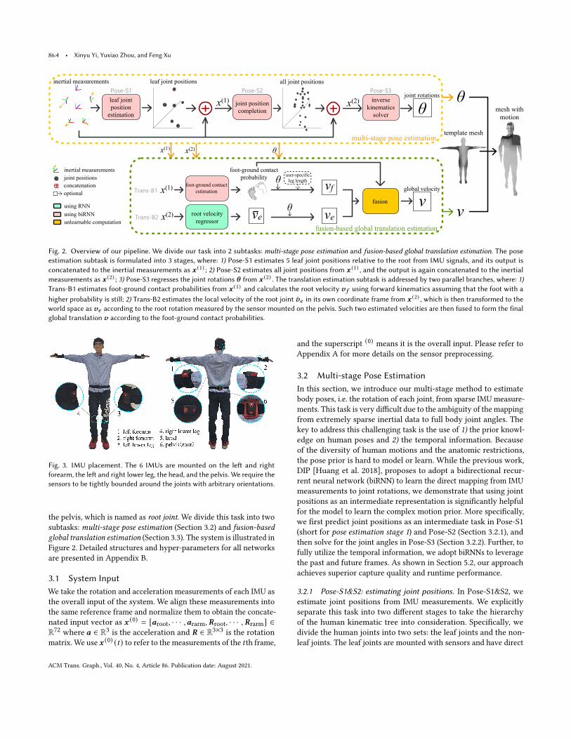
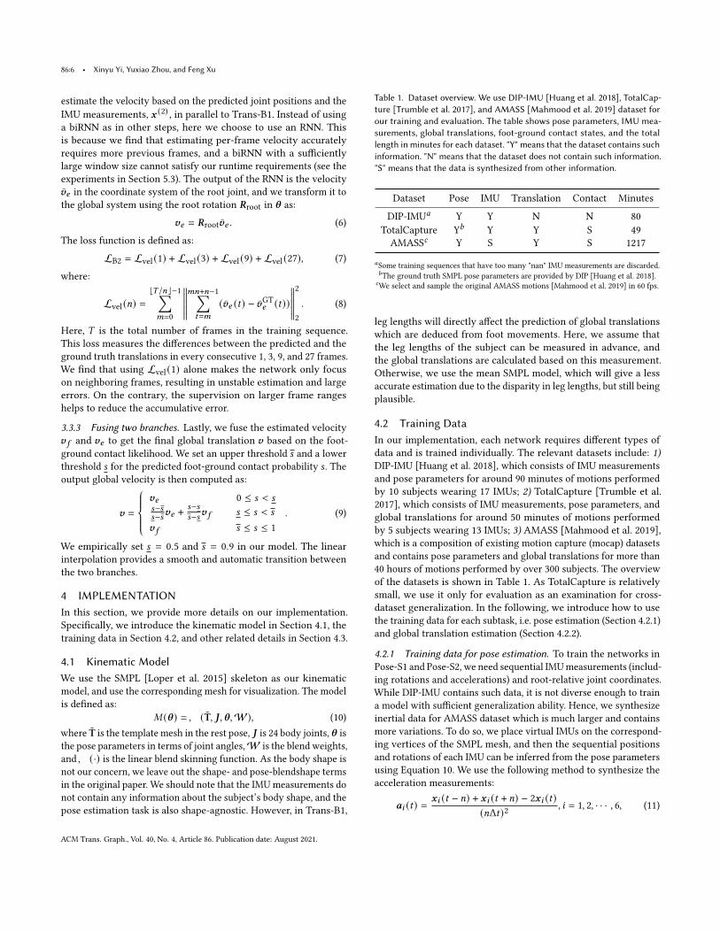
Fig. 2. Overview of our pipeline. We divide our task into 2 subtasks: multi-stage pose estimation and fusion-based global translation estimation. The poseestimation subtask is formulated into 3 stages, where: 1) Pose-S1 estimates 5 leaf joint positions relative to the root from IMU signals, and its output isconcatenated to the inertial measurements as 𝒙 (1) ; 2) Pose-S2 estimates all joint positions from 𝒙 (1) , and the output is again concatenated to the inertialmeasurements as 𝒙 (2) ; 3) Pose-S3 regresses the joint rotations 𝜽 from 𝒙 (2) . The translation estimation subtask is addressed by two parallel branches, where: 1)Trans-B1 estimates foot-ground contact probabilities from 𝒙 (1) and calculates the root velocity 𝒗 𝑓 using forward kinematics assuming that the foot with ahigher probability is still; 2) Trans-B2 estimates the local velocity of the root joint �̄�𝑒 in its own coordinate frame from 𝒙 (2) , which is then transformed to theworld space as 𝒗𝑒 according to the root rotation measured by the sensor mounted on the pelvis. Such two estimated velocities are then fused to form the finalglobal translation 𝒗 according to the foot-ground contact probabilities.
Fig. 3. IMU placement. The 6 IMUs are mounted on the left and rightforearm, the left and right lower leg, the head, and the pelvis. We require thesensors to be tightly bounded around the joints with arbitrary orientations.
the pelvis, which is named as root joint. We divide this task into twosubtasks: multi-stage pose estimation (Section 3.2) and fusion-basedglobal translation estimation (Section 3.3). The system is illustrated inFigure 2. Detailed structures and hyper-parameters for all networksare presented in Appendix B.
3.1 System InputWe take the rotation and acceleration measurements of each IMU asthe overall input of the system. We align these measurements intothe same reference frame and normalize them to obtain the concate-nated input vector as 𝒙 (0) = [𝒂root, · · · , 𝒂rarm, 𝑹root, · · · , 𝑹rarm] ∈R72 where 𝒂 ∈ R3 is the acceleration and 𝑹 ∈ R3×3 is the rotationmatrix. We use 𝒙 (0) (𝑡) to refer to the measurements of the 𝑡 th frame,
and the superscript (0) means it is the overall input. Please refer toAppendix A for more details on the sensor preprocessing.
3.2 Multi-stage Pose EstimationIn this section, we introduce our multi-stage method to estimatebody poses, i.e. the rotation of each joint, from sparse IMU measure-ments. This task is very difficult due to the ambiguity of the mappingfrom extremely sparse inertial data to full body joint angles. Thekey to address this challenging task is the use of 1) the prior knowl-edge on human poses and 2) the temporal information. Becauseof the diversity of human motions and the anatomic restrictions,the pose prior is hard to model or learn. While the previous work,DIP [Huang et al. 2018], proposes to adopt a bidirectional recur-rent neural network (biRNN) to learn the direct mapping from IMUmeasurements to joint rotations, we demonstrate that using jointpositions as an intermediate representation is significantly helpfulfor the model to learn the complex motion prior. More specifically,we first predict joint positions as an intermediate task in Pose-S1(short for pose estimation stage 1) and Pose-S2 (Section 3.2.1), andthen solve for the joint angles in Pose-S3 (Section 3.2.2). Further, tofully utilize the temporal information, we adopt biRNNs to leveragethe past and future frames. As shown in Section 5.2, our approachachieves superior capture quality and runtime performance.
3.2.1 Pose-S1&S2: estimating joint positions. In Pose-S1&S2, weestimate joint positions from IMU measurements. We explicitlyseparate this task into two different stages to take the hierarchyof the human kinematic tree into consideration. Specifically, wedivide the human joints into two sets: the leaf joints and the non-leaf joints. The leaf joints are mounted with sensors and have direct
ACM Trans. Graph., Vol. 40, No. 4, Article 86. Publication date: August 2021.
TransPose: Real-time 3D Human Translation and Pose Estimation with Six Inertial Sensors • 86:5
measurements. Usually, they have larger movements. The inner non-leaf joints are without any direct inertial data and have relativelysmaller motions. Due to the correlation between body joints, theinformation of the leaf joints is helpful for predicting the coordinatesof inner ones. We first regress the positions of the leaf joints in Pose-S1, and then localize the other joints in Pose-S2.The input to Pose-S1 is the inertial measurement vector 𝒙 (0) (𝑡),
and the output is the root-relative positions of the five leaf joints𝒑leaf (𝑡) = [𝒑lleg (𝑡), · · · ,𝒑rarm (𝑡)] ∈ R15. We use a standard biRNN[Schuster and Paliwal 1997] with Long Short-Term Memory (LSTM)cells [Hochreiter and Schmidhuber 1997] to learn the mapping fromIMU measurements to leaf joint positions. Due to the very sparsemeasurements, it is common that the IMUs show identical signalswhile the subject is performing different animations. For example,when sitting still or standing still, the acceleration and orientationmeasurements of all the IMUs are almost the same. In such cases,the temporal information is the key to resolve this ambiguity, thususing RNNs is a natural choice. We choose to use biRNNs insteadof vanilla RNNs because the future information is also of great helpin this task, as stated in DIP. The loss function used to train thenetwork is defined as:
LS1 = ∥𝒑leaf (𝑡) − 𝒑GTleaf (𝑡)∥
22 , (1)
where superscript GT denotes the ground truth.The input of Pose-S2 is the concatenation of Pose-S1’s output
and the inertial measurements: 𝒙 (1) (𝑡) = [𝒑leaf (𝑡), 𝒙 (0) (𝑡)] ∈ R87.Based on the input information, Pose-S2 outputs the root-relativecoordinates of all joints: 𝒑all (𝑡) = [𝒑 𝑗 (𝑡) | 𝑗 = 1, 2, · · · , 𝐽 − 1] ∈R3( 𝐽 −1) , where 𝐽 is the number of joints in the human kinematictree. Similar to Pose-S1, we use a biRNN for Pose-S2 with L2 loss:
LS2 = ∥𝒑all (𝑡) − 𝒑GTall (𝑡)∥
22 . (2)
3.2.2 Pose-S3: estimating joint rotations. In Pose-S3, we estimatejoint rotations from joint positions. We concatenate the joint coordi-nates and the inertial measurements as 𝒙 (2) (𝑡) = [𝒑all (𝑡), 𝒙 (0) (𝑡)] ∈R3( 𝐽 −1)+72, which is the input of Pose-S3. The input vector is fedinto a biRNN, which predicts the rotations of all non-root jointsrelative to the root in the 6D representation [Zhou et al. 2018]:𝑹 (6D)all (𝑡) = [𝑹 (6D)
𝑗(𝑡) | 𝑗 = 1, 2, · · · , 𝐽 − 1] ∈ R6( 𝐽 −1) . We choose the
6D rotation representation over other common representations suchas quaternions as the output for better continuity, as demonstratedin [Zhou et al. 2018]. We should note that the IMU measurementsare fed into the networks as rotation matrices, while the only use ofthe 6D representation is in the output of Pose-S3. The loss functionis defined as:
LS3 = ∥𝑹 (6D)all (𝑡) − 𝑹GT,(6D)
all (𝑡)∥22 . (3)
The rotation of the root joint 𝑹root is directly measured by the sensorplaced on the pelvis. Combining all these rotations, we convert themto the rotation matrix formulation and obtain the full body pose as𝜽 = [𝑹 𝑗 (𝑡) | 𝑗 = 0, 1, · · · , 𝐽 ] ∈ R9𝐽 .
3.3 Fusion-based Global Translation EstimationIn this section, we explain ourmethod to estimate global translationsfrom the IMU measurements and the estimated body poses. This
task is even more challenging due to the lack of direct distancemeasurements, and the acceleration measurements are too noisyto be used directly [Marcard et al. 2017]. Previous works addressthis task by introducing additional vision inputs [Andrews et al.2016; Henschel et al. 2020; Malleson et al. 2019, 2017] or distancemeasurements [Liu et al. 2011; Vlasic et al. 2007], which increase thecomplexity of the system.While thework of SIP [Marcard et al. 2017]estimates global translations from IMUs only, it has to run in anoffline manner. To our best knowledge, we are the first method thataddresses the task of real-time prediction of global translations fromsparse IMUs. To do so, we need to estimate the per-frame velocity ofthe root joint, i.e. the translation between the current frame and theprevious frame. We propose a fusion-based approach that comprisestwo parallel branches. In Trans-B1 (short for translation estimationbranch 1) (Section 3.3.1), we infer the root velocity based on thesequential pose estimation, in combination with the prediction offoot-ground contact probabilities. In Trans-B2 (Section 3.3.2), weuse an RNN to predict the root velocity from joint positions andinertial measurements. These two branches run in a parallel style,and the final estimation is a fusion of the two branches based on thefoot state (Section 3.3.3). The intuition behind is that by assumingthe foot on the ground is not moving, the per-frame velocity can bededuced from the motion of the subject. However, this estimation isnot totally accurate and inevitably fails when both feet are not onthe ground, e.g., jumping or running. Therefore, a neural network isused here for complementary estimation.We demonstrate in Section5.3 that such a hybrid approach gives more accurate results thanusing either branch alone.
3.3.1 Trans-B1: supporting-foot-based velocity estimation. In Trans-B1, we estimate the velocity of the root joint based on the estimationof body poses. First, we use a biRNN to estimate the foot-groundcontact probability for each foot, i.e. the likelihood that the footis on the ground, formulated as 𝒔foot = [𝑠lfoot, 𝑠rfoot] ∈ R2. Theinput of this network is the leaf joint positions and the inertialmeasurements, 𝒙 (1) . We assume that the foot with a higher on-ground probability is not moving between two adjacent frames,referred to as the supporting foot. The corresponding probability isdenoted as 𝑠 = max{𝑠lfoot, 𝑠rfoot}. Then, we apply the estimated poseparameters 𝜽 on the kinematic model with optional user-specificleg lengths 𝒍 , and the root velocity is essentially the coordinatedifference of the supporting foot between two consecutive frames,denoted as 𝒗 𝑓 :
𝒗 𝑓 (𝑡) = FK(𝜽 (𝑡 − 1); 𝒍) − FK(𝜽 (𝑡); 𝒍), (4)
where FK(·) is the forward kinematics function that calculates theposition of the supporting foot from the pose parameters. To trainthe model, we use a cross-entropy loss defined as:
LB1 = − 𝑠GTlfoot log 𝑠lfoot − (1 − 𝑠GTlfoot) log(1 − 𝑠lfoot)
− 𝑠GTrfoot log 𝑠rfoot − (1 − 𝑠GTrfoot) log(1 − 𝑠rfoot) .(5)
3.3.2 Trans-B2: network-based velocity estimation. While the pose-based method in Trans-B1 is straightforward, it is substantiallyincapable of the cases where both feet are off the ground simultane-ously. Further, the errors in the pose estimation will also affect theaccuracy. To this end, we additionally adopt a neural network to
ACM Trans. Graph., Vol. 40, No. 4, Article 86. Publication date: August 2021.
86:6 • Xinyu Yi, Yuxiao Zhou, and Feng Xu
estimate the velocity based on the predicted joint positions and theIMU measurements, 𝒙 (2) , in parallel to Trans-B1. Instead of usinga biRNN as in other steps, here we choose to use an RNN. Thisis because we find that estimating per-frame velocity accuratelyrequires more previous frames, and a biRNN with a sufficientlylarge window size cannot satisfy our runtime requirements (see theexperiments in Section 5.3). The output of the RNN is the velocity𝒗𝑒 in the coordinate system of the root joint, and we transform it tothe global system using the root rotation 𝑹root in 𝜽 as:
𝒗𝑒 = 𝑹root𝒗𝑒 . (6)
The loss function is defined as:
LB2 = Lvel (1) + Lvel (3) + Lvel (9) + Lvel (27), (7)
where:
Lvel (𝑛) =⌊𝑇 /𝑛⌋−1∑𝑚=0
𝑚𝑛+𝑛−1∑𝑡=𝑚
(𝒗𝑒 (𝑡) − 𝒗GT𝑒 (𝑡)) 22. (8)
Here, 𝑇 is the total number of frames in the training sequence.This loss measures the differences between the predicted and theground truth translations in every consecutive 1, 3, 9, and 27 frames.We find that using Lvel (1) alone makes the network only focuson neighboring frames, resulting in unstable estimation and largeerrors. On the contrary, the supervision on larger frame rangeshelps to reduce the accumulative error.
3.3.3 Fusing two branches. Lastly, we fuse the estimated velocity𝒗 𝑓 and 𝒗𝑒 to get the final global translation 𝒗 based on the foot-ground contact likelihood. We set an upper threshold 𝑠 and a lowerthreshold 𝑠 for the predicted foot-ground contact probability 𝑠 . Theoutput global velocity is then computed as:
𝒗 =
𝒗𝑒 0 ≤ 𝑠 < 𝑠𝑠−𝑠𝑠−𝑠 𝒗𝑒 +
𝑠−𝑠𝑠−𝑠 𝒗 𝑓 𝑠 ≤ 𝑠 < 𝑠
𝒗 𝑓 𝑠 ≤ 𝑠 ≤ 1. (9)
We empirically set 𝑠 = 0.5 and 𝑠 = 0.9 in our model. The linearinterpolation provides a smooth and automatic transition betweenthe two branches.
4 IMPLEMENTATIONIn this section, we provide more details on our implementation.Specifically, we introduce the kinematic model in Section 4.1, thetraining data in Section 4.2, and other related details in Section 4.3.
4.1 Kinematic ModelWe use the SMPL [Loper et al. 2015] skeleton as our kinematicmodel, and use the corresponding mesh for visualization. The modelis defined as:
𝑀 (𝜽 ) =𝑊 (T̄, 𝑱 , 𝜽 ,W), (10)where T̄ is the template mesh in the rest pose, 𝑱 is 24 body joints, 𝜽 isthe pose parameters in terms of joint angles,W is the blend weights,and𝑊 (·) is the linear blend skinning function. As the body shape isnot our concern, we leave out the shape- and pose-blendshape termsin the original paper. We should note that the IMUmeasurements donot contain any information about the subject’s body shape, and thepose estimation task is also shape-agnostic. However, in Trans-B1,
Table 1. Dataset overview. We use DIP-IMU [Huang et al. 2018], TotalCap-ture [Trumble et al. 2017], and AMASS [Mahmood et al. 2019] dataset forour training and evaluation. The table shows pose parameters, IMU mea-surements, global translations, foot-ground contact states, and the totallength in minutes for each dataset. "Y" means that the dataset contains suchinformation. "N" means that the dataset does not contain such information."S" means that the data is synthesized from other information.
Dataset Pose IMU Translation Contact Minutes
DIP-IMUa Y Y N N 80TotalCapture Yb Y Y S 49AMASSc Y S Y S 1217
aSome training sequences that have too many "nan" IMU measurements are discarded.bThe ground truth SMPL pose parameters are provided by DIP [Huang et al. 2018].cWe select and sample the original AMASS motions [Mahmood et al. 2019] in 60 fps.
leg lengths will directly affect the prediction of global translationswhich are deduced from foot movements. Here, we assume thatthe leg lengths of the subject can be measured in advance, andthe global translations are calculated based on this measurement.Otherwise, we use the mean SMPL model, which will give a lessaccurate estimation due to the disparity in leg lengths, but still beingplausible.
4.2 Training DataIn our implementation, each network requires different types ofdata and is trained individually. The relevant datasets include: 1)DIP-IMU [Huang et al. 2018], which consists of IMU measurementsand pose parameters for around 90 minutes of motions performedby 10 subjects wearing 17 IMUs; 2) TotalCapture [Trumble et al.2017], which consists of IMU measurements, pose parameters, andglobal translations for around 50 minutes of motions performedby 5 subjects wearing 13 IMUs; 3) AMASS [Mahmood et al. 2019],which is a composition of existing motion capture (mocap) datasetsand contains pose parameters and global translations for more than40 hours of motions performed by over 300 subjects. The overviewof the datasets is shown in Table 1. As TotalCapture is relativelysmall, we use it only for evaluation as an examination for cross-dataset generalization. In the following, we introduce how to usethe training data for each subtask, i.e. pose estimation (Section 4.2.1)and global translation estimation (Section 4.2.2).
4.2.1 Training data for pose estimation. To train the networks inPose-S1 and Pose-S2, we need sequential IMUmeasurements (includ-ing rotations and accelerations) and root-relative joint coordinates.While DIP-IMU contains such data, it is not diverse enough to traina model with sufficient generalization ability. Hence, we synthesizeinertial data for AMASS dataset which is much larger and containsmore variations. To do so, we place virtual IMUs on the correspond-ing vertices of the SMPL mesh, and then the sequential positionsand rotations of each IMU can be inferred from the pose parametersusing Equation 10. We use the following method to synthesize theacceleration measurements:
𝒂𝑖 (𝑡) =𝒙𝑖 (𝑡 − 𝑛) + 𝒙𝑖 (𝑡 + 𝑛) − 2𝒙𝑖 (𝑡)
(𝑛Δ𝑡)2, 𝑖 = 1, 2, · · · , 6, (11)
ACM Trans. Graph., Vol. 40, No. 4, Article 86. Publication date: August 2021.
TransPose: Real-time 3D Human Translation and Pose Estimation with Six Inertial Sensors • 86:7
where 𝒙𝑖 (𝑡) denotes the coordinate of the 𝑖th IMU at frame 𝑡 , 𝒂𝑖 (𝑡) ∈R3 is the acceleration of IMU 𝑖 at frame 𝑡 , and Δ𝑡 is the time intervalbetween two consecutive frames. To cope with jitters in the data,we do not compute the accelerations based on adjacent frames (i.e.𝑛 = 1), but use relatively apart frames for smoother accelerationsby setting 𝑛 = 4. Please refer to Appendix C for more details. Wesynthesize a subset of AMASS dataset which consists of about 1217minutes of motions in 60 fps, which sufficiently cover the motionvariations. To make Pose-S2 robust to the prediction errors of leaf-joint positions, during training, we further add Gaussian noise tothe leaf-joint positions with 𝜎 = 0.04. We use DIP-IMU and syn-thetic AMASS as training datasets for the pose estimation task, andleave TotalCapture for evaluation. To train Pose-S3, we need inertialmeasurements and mocap data in the form of joint angles. We againuse DIP-IMU and synthetic AMASS dataset for Pose-S3 with addi-tional Gaussian noise added to the joint positions, whose standarddeviation is empirically set to 𝜎 = 0.025.
4.2.2 Training data for translation estimation. In Trans-B1, a biRNNis used to predict foot-ground contact probabilities, thus we needbinary annotations for foot-ground contact states. To generate suchdata, we apply the 60-fps pose parameters and root translations onthe SMPL model to obtain the coordinates of both feet, denoted as𝒙 lfoot (𝑡) and 𝒙rfoot (𝑡) for frame 𝑡 . When the movement of one footbetween two consecutive frames is less than a threshold 𝑢, we markit as contacting the ground. We empirically set 𝑢 = 0.008 meters. Inthis way, we automatically label AMASS dataset using:
𝑠GTlfoot (𝑡) ={
1 if ∥𝒙 lfoot (𝑡) − 𝒙 lfoot (𝑡 − 1)∥2 < 𝑢
0 otherwise , (12)
𝑠GTrfoot (𝑡) ={
1 if ∥𝒙rfoot (𝑡) − 𝒙rfoot (𝑡 − 1)∥2 < 𝑢
0 otherwise , (13)
where 𝑠GTlfoot (𝑡) and 𝑠GTrfoot (𝑡) are the foot-ground contact state labels
for frame 𝑡 . For better robustness, we additionally apply Gaussiannoise to the input of Trans-B1 during training, with the standarddeviation set to 𝜎 = 0.04. Since DIP-IMU does not contain globaltranslations, we only use synthetic 60-fps AMASS as the trainingdataset and leave TotalCapture for evaluation.In Trans-B2, an RNN is used to predict the velocity of the root
joint in its own coordinate system. Since the root positions arealready provided in AMASS dataset, we compute the velocity andconvert it from the global space into the root space using:
𝒗GT𝑒 (𝑡) = (𝑹GTroot (𝑡))−1 (𝒙GTroot (𝑡) − 𝒙GTroot (𝑡 − 1)), (14)
where 𝑹GTroot (𝑡) is the ground truth root rotation at frame 𝑡 and
𝒙GTroot (𝑡) is the ground truth root position in world space at frame𝑡 . Note that the frame rate is fixed to be 60 fps for training andtesting, and the velocity is defined as the translation between twoconsecutive 60-fps frames in this paper. We intend to use Trans-B2mainly for the cases where both feet are off the ground, thus we onlyuse such kind of sequences from AMASS to construct the trainingdata. Specifically, we run the well-trained Trans-B1 network andcollect the sequence clips where the minimum foot-ground contactprobability is lower than 𝑠 , i.e. min𝑡 ∈F 𝑠 (𝑡) < 𝑠 , where F is theset containing all frames of the fragment and |F | ≤ 300. During
training, Gaussian noise of 𝜎 = 0.025 is added to the input of Trans-B2.
4.3 Other DetailsAll training and evaluation processes run on a computer with anIntel(R) Core(TM) i7-8700 CPU and an NVIDIA GTX1080Ti graphicscard. The live demo runs on a laptop with an Intel(R) Core(TM) i7-10750H CPU and an NVIDIA RTX2080 Super graphics card. Themodel is implemented using PyTorch 1.7.0 with CUDA 10.1. Thefront end of our live demo is implemented using Unity3D, andwe use Noitom3 Legacy IMU sensors to collect our own data. Weseparately train each network with the batch size of 256 usingan Adam [Kingma and Ba 2014] optimizer with a learning ratelr = 10−3. We follow DIP to train the models for the pose estimationtask using synthetic AMASS first and fine-tune them on DIP-IMUwhich contains real IMU measurements. To avoid the vertical driftdue to the error accumulation in the estimation of translations, weadd a gravity velocity 𝑣𝐺 = 0.018 to the Trans-B1 output 𝒗 𝑓 to pullthe body down.
5 EXPERIMENTSIn this section, we first introduce the data and metrics used in ourexperiments in Section 5.1. Using the data and metrics, we compareour method with previous methods qualitatively and quantitativelyin Section 5.2. Next, we evaluate our important design choices andkey technical components by ablative studies in Section 5.3. Finally,to further demonstrate the power of our technique, we show variousreal-time results containing strong occlusion, wide range motionspace, dark and outdoor environment, close interaction, andmultipleusers in Section 5.4. Following DIP [Huang et al. 2018], we adopttwo settings of inference: the offline setting where the full sequenceis available at the test time, and the online (real-time) setting whereour approach accesses 20 past frames, 1 current frame, and 5 futureframes in a window sliding manner, with a tolerable latency of83ms. Please note that all the results are estimated from the realIMU measurements, and no temporal filter is used in our method.Following DIP, we do not give rotation freedoms to the wrists andankles because we have no observation to solve them.
5.1 Data and MetricsThe pose evaluations are conducted on the test split of DIP-IMU[Huang et al. 2018] and TotalCapture [Trumble et al. 2017] dataset.The global translation evaluations are conducted on TotalCapturealone, as DIP-IMU does not contain global movements. We use thefollowing metrics for quantitative evaluations of poses: 1) SIP errormeasures the mean global rotation error of upper arms and upperlegs in degrees; 2) angular error measures the mean global rotationerror of all body joints in degrees; 3) positional error measures themean Euclidean distance error of all estimated joints in centimeterswith the root joint (Spine) aligned; 4) mesh error measures the meanEuclidean distance error of all vertices of the estimated body meshalso with the root joint (Spine) aligned. The vertex coordinates arecalculated by applying the pose parameters to the SMPL [Loper et al.2015] body model with the mean shape using Equation 10. Note
3https://www.noitom.com/
ACM Trans. Graph., Vol. 40, No. 4, Article 86. Publication date: August 2021.
86:8 • Xinyu Yi, Yuxiao Zhou, and Feng Xu
that the errors in twisting (rotations around the bone) cannot bemeasured by positional error, but will be reflected in mesh error.5) Jitter error measures the average jerk of all body joints in thepredicted motion. Jerk is the third derivative of position with respectto time and reflects the smoothness and naturalness of the motion[Flash and Hogan 1985]. A smaller average jerk means a smootherand more natural animation.
5.2 ComparisonsQuantitative and qualitative comparisons with DIP [Huang et al.2018] and SIP/SOP (SOP is a simplified version of SIP that only usesorientation measurements) [Marcard et al. 2017] are conducted andthe results are shown in this section. We should note that our testdata is slightly different from [Huang et al. 2018] for both DIP-IMUand TotalCapture, resulting in some inconsistency with the valuesreported by DIP. More specifically, the DIP-IMU dataset containsboth raw and calibrated data, and the results in the DIP paper arebased on the latter. However, the calibrated data removes the rootinertial measurements which are required by our method to estimatethe global motions, so we have to perform the comparisons on theraw data. As for the TotalCapture dataset, the ground truth SMPLpose parameters are acquired from the DIP authors. To evaluate DIPon the test data, we use the DIP model and the code released by theauthors. No temporal filtering technique is applied.
5.2.1 Quantitative comparisons. The quantitative comparisons areshown in Table 2 for the offline setting and Table 3 for the onlinesetting. We report the mean and standard deviation for each metricin comparison with DIP (both offline and online) and SIP/SOP (onlyoffline). As shown in the tables, our method outperforms all previousworks in all metrics. We attribute our superiority to the multi-stagestructure that first estimates joint coordinates in the positional spaceand then solves for the angles in the rotational space. We argue thathuman poses are easier to estimate in the joint-coordinate space,and with the help of the coordinates, joint rotations can be betterestimated. A fly in the ointment is that we can see an accuracy gapbetween online and offline settings. The reason is that the offlinesetting uses much more temporal information to solve the pose ofthe current frame, while the online setting does not do this to avoidnoticeable delay. Since our approach fully exploits such temporalinformation to resolve the motion ambiguities, there is an inevitableaccuracy reduction when switching from the offline setting to theonline setting. Nevertheless, we still achieve the state-of-the-artonline capture quality which is visually pleasing as shown in thequalitative results and the live demos.
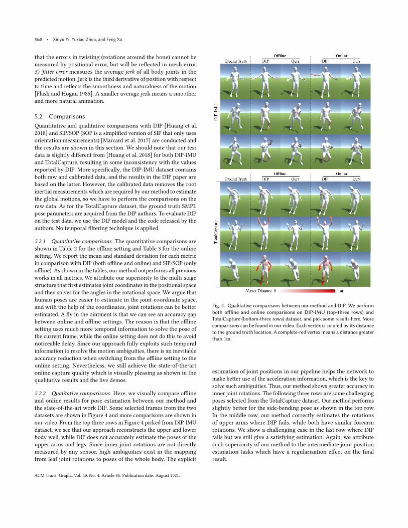
5.2.2 Qualitative comparisons. Here, we visually compare offlineand online results for pose estimation between our method andthe state-of-the-art work DIP. Some selected frames from the twodatasets are shown in Figure 4 and more comparisons are shown inour video. From the top three rows in Figure 4 picked from DIP-IMUdataset, we see that our approach reconstructs the upper and lowerbody well, while DIP does not accurately estimate the poses of theupper arms and legs. Since inner joint rotations are not directlymeasured by any sensor, high ambiguities exist in the mappingfrom leaf joint rotations to poses of the whole body. The explicit
Fig. 4. Qualitative comparisons between our method and DIP. We performboth offline and online comparisons on DIP-IMU (top-three rows) andTotalCapture (bottom-three rows) dataset, and pick some results here. Morecomparisons can be found in our video. Each vertex is colored by its distanceto the ground truth location. A complete-red vertex means a distance greaterthan 1m.
estimation of joint positions in our pipeline helps the network tomake better use of the acceleration information, which is the key tosolve such ambiguities. Thus, our method shows greater accuracy ininner joint rotations. The following three rows are some challengingposes selected from the TotalCapture dataset. Our method performsslightly better for the side-bending pose as shown in the top row.In the middle row, our method correctly estimates the rotationsof upper arms where DIP fails, while both have similar forearmrotations. We show a challenging case in the last row where DIPfails but we still give a satisfying estimation. Again, we attributesuch superiority of our method to the intermediate joint positionestimation tasks which have a regularization effect on the finalresult.
ACM Trans. Graph., Vol. 40, No. 4, Article 86. Publication date: August 2021.
TransPose: Real-time 3D Human Translation and Pose Estimation with Six Inertial Sensors • 86:9
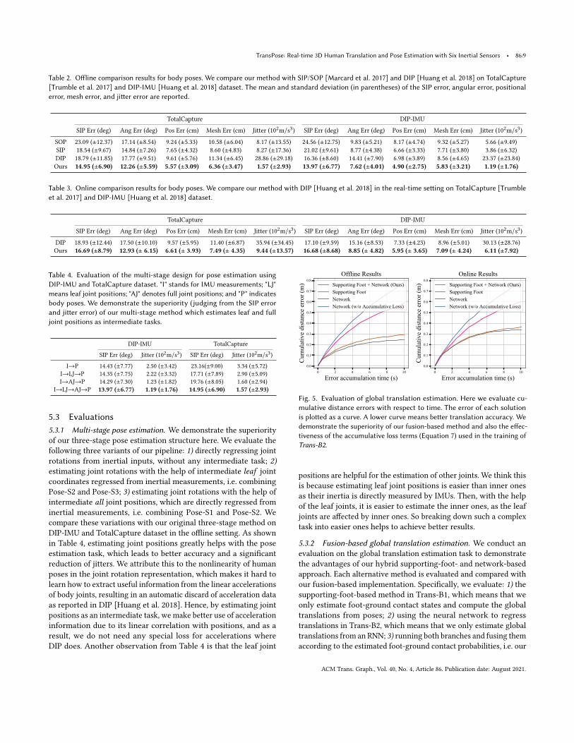
Table 2. Offline comparison results for body poses. We compare our method with SIP/SOP [Marcard et al. 2017] and DIP [Huang et al. 2018] on TotalCapture[Trumble et al. 2017] and DIP-IMU [Huang et al. 2018] dataset. The mean and standard deviation (in parentheses) of the SIP error, angular error, positionalerror, mesh error, and jitter error are reported.
TotalCapture DIP-IMU
SIP Err (deg) Ang Err (deg) Pos Err (cm) Mesh Err (cm) Jitter (102m/s3) SIP Err (deg) Ang Err (deg) Pos Err (cm) Mesh Err (cm) Jitter (102m/s3)SOP 23.09 (±12.37) 17.14 (±8.54) 9.24 (±5.33) 10.58 (±6.04) 8.17 (±13.55) 24.56 (±12.75) 9.83 (±5.21) 8.17 (±4.74) 9.32 (±5.27) 5.66 (±9.49)SIP 18.54 (±9.67) 14.84 (±7.26) 7.65 (±4.32) 8.60 (±4.83) 8.27 (±17.36) 21.02 (±9.61) 8.77 (±4.38) 6.66 (±3.33) 7.71 (±3.80) 3.86 (±6.32)DIP 18.79 (±11.85) 17.77 (±9.51) 9.61 (±5.76) 11.34 (±6.45) 28.86 (±29.18) 16.36 (±8.60) 14.41 (±7.90) 6.98 (±3.89) 8.56 (±4.65) 23.37 (±23.84)Ours 14.95 (±6.90) 12.26 (±5.59) 5.57 (±3.09) 6.36 (±3.47) 1.57 (±2.93) 13.97 (±6.77) 7.62 (±4.01) 4.90 (±2.75) 5.83 (±3.21) 1.19 (±1.76)
Table 3. Online comparison results for body poses. We compare our method with DIP [Huang et al. 2018] in the real-time setting on TotalCapture [Trumbleet al. 2017] and DIP-IMU [Huang et al. 2018] dataset.
TotalCapture DIP-IMU
SIP Err (deg) Ang Err (deg) Pos Err (cm) Mesh Err (cm) Jitter (102m/s3) SIP Err (deg) Ang Err (deg) Pos Err (cm) Mesh Err (cm) Jitter (102m/s3)DIP 18.93 (±12.44) 17.50 (±10.10) 9.57 (±5.95) 11.40 (±6.87) 35.94 (±34.45) 17.10 (±9.59) 15.16 (±8.53) 7.33 (±4.23) 8.96 (±5.01) 30.13 (±28.76)Ours 16.69 (±8.79) 12.93 (± 6.15) 6.61 (± 3.93) 7.49 (± 4.35) 9.44 (±13.57) 16.68 (±8.68) 8.85 (± 4.82) 5.95 (± 3.65) 7.09 (± 4.24) 6.11 (±7.92)
Table 4. Evaluation of the multi-stage design for pose estimation usingDIP-IMU and TotalCapture dataset. "I" stands for IMU measurements; "LJ"means leaf joint positions; "AJ" denotes full joint positions; and "P" indicatesbody poses. We demonstrate the superiority (judging from the SIP errorand jitter error) of our multi-stage method which estimates leaf and fulljoint positions as intermediate tasks.
DIP-IMU TotalCapture
SIP Err (deg) Jitter (102m/s3) SIP Err (deg) Jitter (102m/s3)I→P 14.43 (±7.77) 2.50 (±3.42) 23.16(±9.00) 3.34 (±5.72)
I→LJ→P 14.35 (±7.75) 2.22 (±3.32) 17.71 (±7.89) 2.90 (±5.09)I→AJ→P 14.29 (±7.30) 1.23 (±1.82) 19.76 (±8.05) 1.60 (±2.94)
I→LJ→AJ→P 13.97 (±6.77) 1.19 (±1.76) 14.95 (±6.90) 1.57 (±2.93)
5.3 Evaluations5.3.1 Multi-stage pose estimation. We demonstrate the superiorityof our three-stage pose estimation structure here. We evaluate thefollowing three variants of our pipeline: 1) directly regressing jointrotations from inertial inputs, without any intermediate task; 2)estimating joint rotations with the help of intermediate leaf jointcoordinates regressed from inertial measurements, i.e. combiningPose-S2 and Pose-S3; 3) estimating joint rotations with the help ofintermediate all joint positions, which are directly regressed frominertial measurements, i.e. combining Pose-S1 and Pose-S2. Wecompare these variations with our original three-stage method onDIP-IMU and TotalCapture dataset in the offline setting. As shownin Table 4, estimating joint positions greatly helps with the poseestimation task, which leads to better accuracy and a significantreduction of jitters. We attribute this to the nonlinearity of humanposes in the joint rotation representation, which makes it hard tolearn how to extract useful information from the linear accelerationsof body joints, resulting in an automatic discard of acceleration dataas reported in DIP [Huang et al. 2018]. Hence, by estimating jointpositions as an intermediate task, we make better use of accelerationinformation due to its linear correlation with positions, and as aresult, we do not need any special loss for accelerations whereDIP does. Another observation from Table 4 is that the leaf joint
0 2 4 6 8 10
Error accumulation time (s)
0.0
0.1
0.2
0.3
0.4
0.5
0.6
0.7
0.8
Cum
ulat
ive
dist
ance
err
or (m
)
Offline ResultsSupporting Foot + Network (Ours)Supporting FootNetworkNetwork (w/o Accumulative Loss)
0 2 4 6 8 10
Error accumulation time (s)
0.0
0.1
0.2
0.3
0.4
0.5
0.6
0.7
0.8
Cum
ulat
ive
dist
ance
err
or (m
)
Online ResultsSupporting Foot + Network (Ours)Supporting FootNetworkNetwork (w/o Accumulative Loss)
Fig. 5. Evaluation of global translation estimation. Here we evaluate cu-mulative distance errors with respect to time. The error of each solutionis plotted as a curve. A lower curve means better translation accuracy. Wedemonstrate the superiority of our fusion-based method and also the effec-tiveness of the accumulative loss terms (Equation 7) used in the training ofTrans-B2.
positions are helpful for the estimation of other joints. We think thisis because estimating leaf joint positions is easier than inner onesas their inertia is directly measured by IMUs. Then, with the helpof the leaf joints, it is easier to estimate the inner ones, as the leafjoints are affected by inner ones. So breaking down such a complextask into easier ones helps to achieve better results.
5.3.2 Fusion-based global translation estimation. We conduct anevaluation on the global translation estimation task to demonstratethe advantages of our hybrid supporting-foot- and network-basedapproach. Each alternative method is evaluated and compared withour fusion-based implementation. Specifically, we evaluate: 1) thesupporting-foot-based method in Trans-B1, which means that weonly estimate foot-ground contact states and compute the globaltranslations from poses; 2) using the neural network to regresstranslations in Trans-B2, which means that we only estimate globaltranslations from an RNN; 3) running both branches and fusing themaccording to the estimated foot-ground contact probabilities, i.e. our
ACM Trans. Graph., Vol. 40, No. 4, Article 86. Publication date: August 2021.
86:10 • Xinyu Yi, Yuxiao Zhou, and Feng Xu
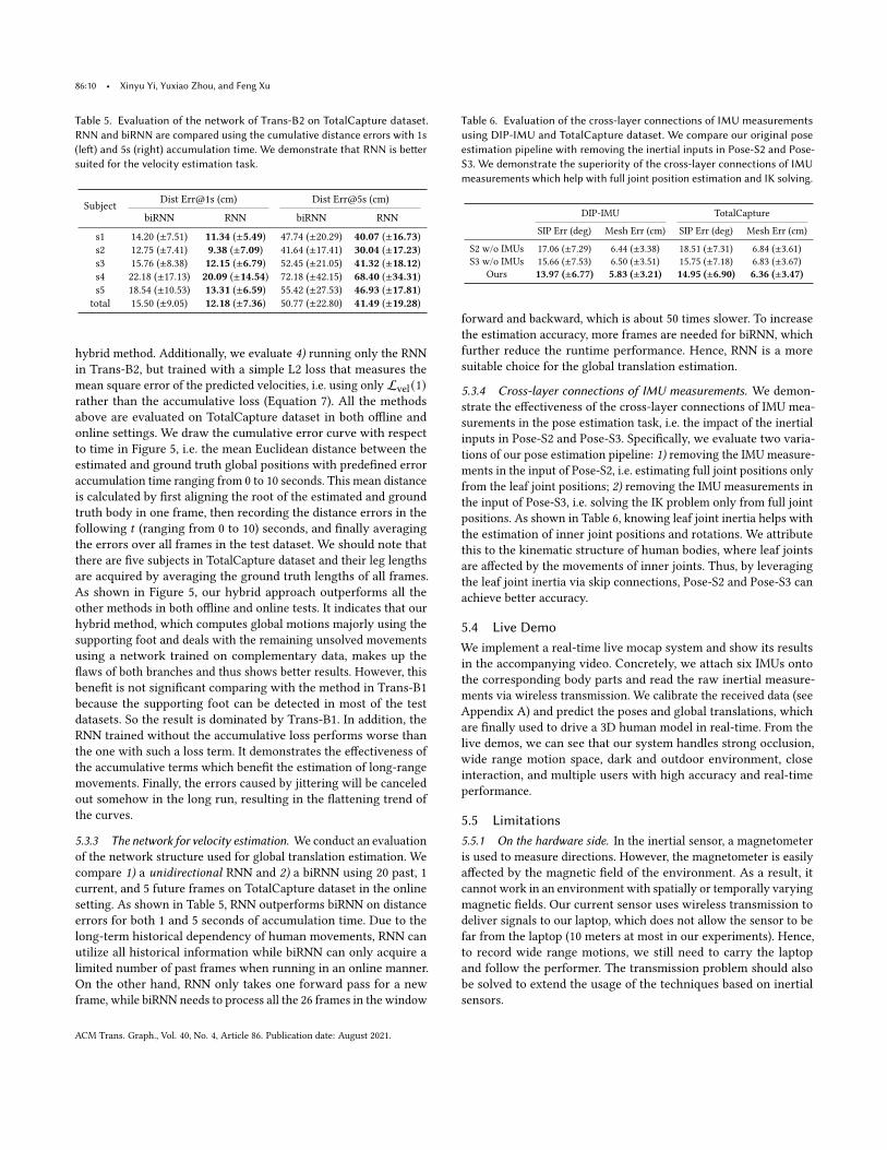
Table 5. Evaluation of the network of Trans-B2 on TotalCapture dataset.RNN and biRNN are compared using the cumulative distance errors with 1s(left) and 5s (right) accumulation time. We demonstrate that RNN is bettersuited for the velocity estimation task.
Subject Dist Err@1s (cm) Dist Err@5s (cm)
biRNN RNN biRNN RNN
s1 14.20 (±7.51) 11.34 (±5.49) 47.74 (±20.29) 40.07 (±16.73)s2 12.75 (±7.41) 9.38 (±7.09) 41.64 (±17.41) 30.04 (±17.23)s3 15.76 (±8.38) 12.15 (±6.79) 52.45 (±21.05) 41.32 (±18.12)s4 22.18 (±17.13) 20.09 (±14.54) 72.18 (±42.15) 68.40 (±34.31)s5 18.54 (±10.53) 13.31 (±6.59) 55.42 (±27.53) 46.93 (±17.81)
total 15.50 (±9.05) 12.18 (±7.36) 50.77 (±22.80) 41.49 (±19.28)
hybrid method. Additionally, we evaluate 4) running only the RNNin Trans-B2, but trained with a simple L2 loss that measures themean square error of the predicted velocities, i.e. using only Lvel (1)rather than the accumulative loss (Equation 7). All the methodsabove are evaluated on TotalCapture dataset in both offline andonline settings. We draw the cumulative error curve with respectto time in Figure 5, i.e. the mean Euclidean distance between theestimated and ground truth global positions with predefined erroraccumulation time ranging from 0 to 10 seconds. This mean distanceis calculated by first aligning the root of the estimated and groundtruth body in one frame, then recording the distance errors in thefollowing 𝑡 (ranging from 0 to 10) seconds, and finally averagingthe errors over all frames in the test dataset. We should note thatthere are five subjects in TotalCapture dataset and their leg lengthsare acquired by averaging the ground truth lengths of all frames.As shown in Figure 5, our hybrid approach outperforms all theother methods in both offline and online tests. It indicates that ourhybrid method, which computes global motions majorly using thesupporting foot and deals with the remaining unsolved movementsusing a network trained on complementary data, makes up theflaws of both branches and thus shows better results. However, thisbenefit is not significant comparing with the method in Trans-B1because the supporting foot can be detected in most of the testdatasets. So the result is dominated by Trans-B1. In addition, theRNN trained without the accumulative loss performs worse thanthe one with such a loss term. It demonstrates the effectiveness ofthe accumulative terms which benefit the estimation of long-rangemovements. Finally, the errors caused by jittering will be canceledout somehow in the long run, resulting in the flattening trend ofthe curves.
5.3.3 The network for velocity estimation. We conduct an evaluationof the network structure used for global translation estimation. Wecompare 1) a unidirectional RNN and 2) a biRNN using 20 past, 1current, and 5 future frames on TotalCapture dataset in the onlinesetting. As shown in Table 5, RNN outperforms biRNN on distanceerrors for both 1 and 5 seconds of accumulation time. Due to thelong-term historical dependency of human movements, RNN canutilize all historical information while biRNN can only acquire alimited number of past frames when running in an online manner.On the other hand, RNN only takes one forward pass for a newframe, while biRNN needs to process all the 26 frames in the window
Table 6. Evaluation of the cross-layer connections of IMU measurementsusing DIP-IMU and TotalCapture dataset. We compare our original poseestimation pipeline with removing the inertial inputs in Pose-S2 and Pose-S3. We demonstrate the superiority of the cross-layer connections of IMUmeasurements which help with full joint position estimation and IK solving.
DIP-IMU TotalCapture
SIP Err (deg) Mesh Err (cm) SIP Err (deg) Mesh Err (cm)
S2 w/o IMUs 17.06 (±7.29) 6.44 (±3.38) 18.51 (±7.31) 6.84 (±3.61)S3 w/o IMUs 15.66 (±7.53) 6.50 (±3.51) 15.75 (±7.18) 6.83 (±3.67)
Ours 13.97 (±6.77) 5.83 (±3.21) 14.95 (±6.90) 6.36 (±3.47)
forward and backward, which is about 50 times slower. To increasethe estimation accuracy, more frames are needed for biRNN, whichfurther reduce the runtime performance. Hence, RNN is a moresuitable choice for the global translation estimation.
5.3.4 Cross-layer connections of IMU measurements. We demon-strate the effectiveness of the cross-layer connections of IMU mea-surements in the pose estimation task, i.e. the impact of the inertialinputs in Pose-S2 and Pose-S3. Specifically, we evaluate two varia-tions of our pose estimation pipeline: 1) removing the IMU measure-ments in the input of Pose-S2, i.e. estimating full joint positions onlyfrom the leaf joint positions; 2) removing the IMU measurements inthe input of Pose-S3, i.e. solving the IK problem only from full jointpositions. As shown in Table 6, knowing leaf joint inertia helps withthe estimation of inner joint positions and rotations. We attributethis to the kinematic structure of human bodies, where leaf jointsare affected by the movements of inner joints. Thus, by leveragingthe leaf joint inertia via skip connections, Pose-S2 and Pose-S3 canachieve better accuracy.
5.4 Live DemoWe implement a real-time live mocap system and show its resultsin the accompanying video. Concretely, we attach six IMUs ontothe corresponding body parts and read the raw inertial measure-ments via wireless transmission. We calibrate the received data (seeAppendix A) and predict the poses and global translations, whichare finally used to drive a 3D human model in real-time. From thelive demos, we can see that our system handles strong occlusion,wide range motion space, dark and outdoor environment, closeinteraction, and multiple users with high accuracy and real-timeperformance.
5.5 Limitations5.5.1 On the hardware side. In the inertial sensor, a magnetometeris used to measure directions. However, the magnetometer is easilyaffected by the magnetic field of the environment. As a result, itcannot work in an environment with spatially or temporally varyingmagnetic fields. Our current sensor uses wireless transmission todeliver signals to our laptop, which does not allow the sensor to befar from the laptop (10 meters at most in our experiments). Hence,to record wide range motions, we still need to carry the laptopand follow the performer. The transmission problem should alsobe solved to extend the usage of the techniques based on inertialsensors.
ACM Trans. Graph., Vol. 40, No. 4, Article 86. Publication date: August 2021.
TransPose: Real-time 3D Human Translation and Pose Estimation with Six Inertial Sensors • 86:11
5.5.2 On the software side. As a data-driven method, our approachalso suffers from the generalization problem. It cannot handle mo-tions that are largely different from the training dataset, e.g., splitsand other complex motions that can only be performed by pro-fessional dancers and players. Our supporting-foot-based methodrelies on the assumption that the supporting foot has no motionin the world coordinate space, which is not true for motions likeskating and sliding.
6 CONCLUSIONThis paper proposes TransPose, a 90-fps motion capture techniquebased on 6 inertial sensors, which reconstructs full human motionsincluding both body poses and global translations. In this technique,a novel multi-stage method is proposed to estimate body poses basedon the idea of reformulating the problem with two intermediatetasks of leaf and full joint position estimations, which leads to alarge improvement over the state-of-the-art on accuracy, temporalconsistency, and runtime performance. For global translation esti-mation, a fusion technique is used to leverage a purely data-drivenmethod and a method involving the motion rules of the supportingfoot and a kinematic body model. By combining data-driven andmotion-rule-driven, the challenging problem of global translation es-timation from noisy sparse inertial sensors is solved in real-time forthe first time to the best of our knowledge. Extensive experimentswith strong occlusion, wide range motion space, dark and outdoorenvironment, close interaction, and multiple users demonstrate therobustness and accuracy of our technique.
ACKNOWLEDGMENTSWe would like to thank Yinghao Huang and the other DIP authorsfor providing the SMPL parameters for TotalCapture dataset and theSIP/SOP results. We would also like to thank Associate ProfessorYebin Liu for the support on the IMU sensors. We also appreciateHao Zhang, Dong Yang, Wenbin Lin, and Rui Qin for the exten-sive help with the live demos. We thank Chengwei Zheng for theproofreading, and the reviewers for their valuable comments. Thiswork was supported by the National Key R&D Program of China2018YFA0704000, the NSFC (No.61822111, 61727808) and BeijingNatural Science Foundation (JQ19015). Feng Xu is the correspondingauthor.
REFERENCESDavid Aha. 1997. Lazy Learning.Sheldon Andrews, Ivan Huerta, Taku Komura, Leonid Sigal, and Kenny Mitchell. 2016.
Real-time Physics-based Motion Capture with Sparse Sensors. 1–10.E.R. Bachmann, Robert Mcghee, Xiaoping Yun, and Michael Zyda. 2002. Inertial and
Magnetic Posture Tracking for Inserting Humans Into Networked Virtual Environ-ments. (01 2002).
Long Chen, Haizhou Ai, Rui Chen, Zijie Zhuang, and Shuang Liu. 2020. Cross-ViewTracking for Multi-Human 3D Pose Estimation at Over 100 FPS. 3276–3285.
Michael Del Rosario, Heba Khamis, Phillip Ngo, andNigel Lovell. 2018. Computationally-Efficient Adaptive Error-State Kalman Filter for Attitude Estimation. IEEE SensorsJournal PP (08 2018), 1–1.
Tamar Flash and Neville Hogan. 1985. The Coordination of Arm Movements: AnExperimentally Confirmed Mathematical Model. The Journal of neuroscience : theofficial journal of the Society for Neuroscience 5 (08 1985), 1688–703.
Eric Foxlin. 1996. Inertial Head-Tracker Sensor Fusion by a Complementary Separate-Bias Kalman Filter. 185 – 194, 267.
Andrew Gilbert, Matthew Trumble, Charles Malleson, Adrian Hilton, and John Collo-mosse. 2018. Fusing Visual and Inertial Sensors with Semantics for 3D Human Pose
Estimation. International Journal of Computer Vision (09 2018), 1–17.Ikhsanul Habibie, Weipeng Xu, Dushyant Mehta, Gerard Pons-Moll, and Christian
Theobalt. 2019. In the Wild Human Pose Estimation Using Explicit 2D Features andIntermediate 3D Representations. 10897–10906.
Julius Hannink, Thomas Kautz, Cristian Pasluosta, Jochen Klucken, and Bjoern Eskofier.2016. Sensor-Based Gait Parameter Extraction With Deep Convolutional NeuralNetworks. IEEE Journal of Biomedical and Health Informatics PP (09 2016).
Thomas Helten, Meinard Müller, Hans-Peter Seidel, and Christian Theobalt. 2013. Real-Time Body Tracking with One Depth Camera and Inertial Sensors. Proceedings ofthe IEEE International Conference on Computer Vision, 1105–1112.
Roberto Henschel, Timo Marcard, and Bodo Rosenhahn. 2020. Accurate Long-TermMultiple People Tracking using Video and Body-Worn IMUs. IEEE Transactions onImage Processing PP (08 2020), 1–1.
Sepp Hochreiter and Jürgen Schmidhuber. 1997. Long Short-term Memory. Neuralcomputation 9 (12 1997), 1735–80.
Daniel Holden. 2018. Robust solving of optical motion capture data by denoising. ACMTransactions on Graphics (TOG) 37, 4 (2018), 1–12.
Yinghao Huang, Manuel Kaufmann, Emre Aksan, Michael Black, Otmar Hilliges, andGerard Pons-Moll. 2018. Deep inertial poser: Learning to reconstruct human posefrom sparse inertial measurements in real time. ACM Transactions on Graphics 37,1–15.
Diederik Kingma and Jimmy Ba. 2014. Adam: A Method for Stochastic Optimization.International Conference on Learning Representations (12 2014).
Huajun Liu, Xiaolin Wei, Jinxiang Chai, Inwoo Ha, and Taehyun Rhee. 2011. Realtimehuman motion control with a small number of inertial sensors. 133–140.
Matthew Loper, Naureen Mahmood, Javier Romero, Gerard Pons-Moll, and Michael J.Black. 2015. SMPL: A Skinned Multi-Person Linear Model. ACM Trans. Graphics(Proc. SIGGRAPH Asia) 34, 6 (Oct. 2015), 248:1–248:16.
Naureen Mahmood, Nima Ghorbani, Nikolaus F. Troje, Gerard Pons-Moll, and Michael J.Black. 2019. AMASS: Archive of Motion Capture as Surface Shapes. In The IEEEInternational Conference on Computer Vision (ICCV).
Charles Malleson, John Collomosse, and Adrian Hilton. 2019. Real-Time Multi-personMotion Capture fromMulti-view Video and IMUs. International Journal of ComputerVision (12 2019).
Charles Malleson, Andrew Gilbert, Matthew Trumble, John Collomosse, Adrian Hilton,and Marco Volino. 2017. Real-Time Full-Body Motion Capture from Video and IMUs.449–457.
Timo Marcard, Gerard Pons-Moll, and Bodo Rosenhahn. 2016. Human Pose Estimationfrom Video and IMUs. IEEE Transactions on Pattern Analysis and Machine Intelligence38 (02 2016), 1–1.
Timo Marcard, Bodo Rosenhahn, Michael Black, and Gerard Pons-Moll. 2017. SparseInertial Poser: Automatic 3D Human Pose Estimation from Sparse IMUs. ComputerGraphics Forum 36(2), Proceedings of the 38th Annual Conference of the EuropeanAssociation for Computer Graphics (Eurographics), 2017 36 (02 2017).
Dushyant Mehta, Oleksandr Sotnychenko, Franziska Mueller, Weipeng Xu, MohamedElgharib, Pascal Fua, Hans-Peter Seidel, Helge Rhodin, Gerard Pons-Moll, and Chris-tian Theobalt. 2020. XNect: real-time multi-person 3D motion capture with a singleRGB camera. ACM Transactions on Graphics 39 (07 2020).
Thomas BMoeslund and Erik Granum. 2001. A survey of computer vision-based humanmotion capture. Computer vision and image understanding 81, 3 (2001), 231–268.
Thomas B Moeslund, Adrian Hilton, and Volker Krüger. 2006. A survey of advancesin vision-based human motion capture and analysis. Computer vision and imageunderstanding 104, 2-3 (2006), 90–126.
Gerard Pons-Moll, Andreas Baak, Juergen Gall, Laura Leal-Taixé, Meinard Müller,Hans-Peter Seidel, and Bodo Rosenhahn. 2011. Outdoor human motion captureusing inverse kinematics and von mises-fisher sampling. Proceedings of the IEEEInternational Conference on Computer Vision 0, 1243–1250.
Gerard Pons-Moll, Andreas Baak, Thomas Helten, Meinard Müller, Hans-Peter Seidel,and Bodo Rosenhahn. 2010. Multisensor-Fusion for 3D Full-Body Human MotionCapture. IEEE Conference on Computer Vision and Pattern Recognition (CVPR), 663–670.
Qaiser Riaz, Tao Guanhong, Björn Krüger, and Andreas Weber. 2015. Motion Recon-struction Using Very Few Accelerometers and Ground Contacts. Graphical Models(04 2015).
Daniel Roetenberg, Hendrik Luinge, Chris Baten, and Peter Veltink. 2005. Compensa-tion of Magnetic Disturbances Improves Inertial and Magnetic Sensing of HumanBody Segment Orientation. Neural Systems and Rehabilitation Engineering, IEEETransactions on 13 (10 2005), 395 – 405.
Martin Schepers, Matteo Giuberti, and G. Bellusci. 2018. Xsens MVN: ConsistentTracking of Human Motion Using Inertial Sensing. (03 2018).
Mike Schuster and Kuldip K Paliwal. 1997. Bidirectional recurrent neural networks.IEEE transactions on Signal Processing 45, 11 (1997), 2673–2681.
Loren Schwarz, Diana Mateus, and Nassir Navab. 2009. Discriminative Human Full-Body Pose Estimation from Wearable Inertial Sensor Data. 159–172.
Soshi Shimada, Vladislav Golyanik,Weipeng Xu, and Christian Theobalt. 2020. PhysCap:physically plausible monocular 3D motion capture in real time. ACM Transactions
ACM Trans. Graph., Vol. 40, No. 4, Article 86. Publication date: August 2021.
86:12 • Xinyu Yi, Yuxiao Zhou, and Feng Xu
on Graphics 39 (11 2020), 1–16.Ronit Slyper and Jessica Hodgins. 2008. Action Capture with Accelerometers. ACM
SIGGRAPH/Eurographics Symposium on Computer Animation, 193–199.Jochen Tautges, Arno Zinke, Björn Krüger, Jan Baumann, Andreas Weber, Thomas
Helten, Meinard Müller, Hans-Peter Seidel, and Bernhard Eberhardt. 2011. MotionReconstruction Using Sparse Accelerometer Data. ACM Transactions on Graphics 30(05 2011), 18.
Denis Tome, Matteo Toso, Lourdes Agapito, and Chris Russell. 2018. Rethinking Pose in3D: Multi-stage Refinement and Recovery for Markerless Motion Capture. 474–483.
Matthew Trumble, Andrew Gilbert, Adrian Hilton, and John Collomosse. 2016. DeepConvolutional Networks for Marker-less Human Pose Estimation from MultipleViews. 1–9.
Matthew Trumble, Andrew Gilbert, Charles Malleson, Adrian Hilton, and John Collo-mosse. 2017. Total Capture: 3D Human Pose Estimation Fusing Video and InertialSensors.
Rachel Vitali, Ryan McGinnis, and Noel Perkins. 2020. Robust Error-State Kalman Filterfor Estimating IMU Orientation. IEEE Sensors Journal (10 2020).
Daniel Vlasic, Rolf Adelsberger, Giovanni Vannucci, John Barnwell, Markus Gross,Wojciech Matusik, and Jovan Popovic. 2007. Practical motion capture in everydaysurroundings. ACM Trans. Graph. 26 (07 2007), 35.
Timo von Marcard, Roberto Henschel, Michael J. Black, Bodo Rosenhahn, and GerardPons-Moll. 2018. Recovering Accurate 3D Human Pose in theWild Using IMUs and aMoving Camera. In Computer Vision - ECCV 2018 - 15th European Conference, Munich,Germany, September 8-14, 2018, Proceedings, Part X (Lecture Notes in ComputerScience), Vittorio Ferrari, Martial Hebert, Cristian Sminchisescu, and Yair Weiss(Eds.), Vol. 11214. 614–631.
Donglai Xiang, Hanbyul Joo, and Yaser Sheikh. 2019. Monocular Total Capture: PosingFace, Body, and Hands in the Wild. 10957–10966.
Lan Xu, Lu Fang, Wei Cheng, Kaiwen Guo, Guyue Zhou, Qionghai Dai, and YebinLiu. 2016. FlyCap: Markerless Motion Capture Using Multiple Autonomous FlyingCameras. IEEE Transactions on Visualization and Computer Graphics PP (10 2016).
Zhe Zhang, Chunyu Wang, Wenhu Qin, and Wenjun Zeng. 2020. Fusing WearableIMUs With Multi-View Images for Human Pose Estimation: A Geometric Approach.2197–2206.
Zerong Zheng, Yu Tao, Hao Li, Kaiwen Guo, Qionghai Dai, Lu Fang, and Yebin Liu.2018. HybridFusion: Real-Time Performance Capture Using a Single Depth Sensorand Sparse IMUs: 15th European Conference, Munich, Germany, September 8–14, 2018,Proceedings, Part IX. 389–406.
Yi Zhou, Connelly Barnes, Jingwan Lu, Jimei Yang, and Hao Li. 2018. On the Continuityof Rotation Representations in Neural Networks. CoRR abs/1812.07035 (2018).arXiv:1812.07035
Yuxiao Zhou, Marc Habermann, Ikhsanul Habibie, Ayush Tewari, Christian Theobalt,and Feng Xu. 2020a. Monocular Real-time Full Body Capture with Inter-part Corre-lations.
Yuxiao Zhou, Marc Habermann, Weipeng Xu, Ikhsanul Habibie, Christian Theobalt,and Feng Xu. 2020b. Monocular Real-Time Hand Shape and Motion Capture UsingMulti-Modal Data. 5345–5354.
Yuliang Zou, Jimei Yang, Duygu Ceylan, Jianming Zhang, Federico Perazzi, and Jia-BinHuang. 2020. Reducing Footskate in Human Motion Reconstruction with GroundContact Constraints. 448–457.
A SENSOR PREPROCESSINGSince each inertial sensor has its own coordinate system, we needto 1) firstly transform the raw inertial measurements into the samereference frame, which is referred to as calibration, and then 2)transform the leaf joint inertia into the root’s space and rescaleit to a suitable size for the network input, which is referred to asnormalization. The sensors can be placed with arbitrary rotationsduring setup, and our method automatically computes the transitionmatrices for each sensor before capturing the motion. This processrequires the subject to keep in T-pose for a few seconds. In thissection, we explain the details of the sensor preprocessing in ourmethod, including the calibration (Section A.1) and the normaliza-tion (Section A.2).
A.1 CalibrationAn inertial measurement unit (IMU) outputs acceleration data rela-tive to the sensor coordinate frame 𝐹𝑆 and orientation data relativeto the global inertial coordinate frame 𝐹 𝐼 . We define the coordinate
frame of the SMPL [Loper et al. 2015] body model as 𝐹𝑀 , and thebasis matrix of 𝐹𝑆 , 𝐹 𝐼 , 𝐹𝑀 as 𝑩𝑆 ,𝑩𝐼 ,𝑩𝑀 respectively, where eachconsists of three column basis vectors. Before capturing motions,we firstly put an IMU with the axes of its sensor coordinate frame𝐹𝑆 aligned with the corresponding axes of the SMPL coordinateframe 𝐹𝑀 , i.e. to place the IMU with its 𝑥-axis left, 𝑦-axis up and𝑧-axis forward in the real world. Then, the orientation measurement𝑷 𝐼𝑀 can be regarded as the transition matrix from 𝐹 𝐼 to 𝐹𝑀 :
𝑩𝑀 = 𝑩𝐼 𝑷 𝐼𝑀 . (15)
Next, we put each IMU onto the corresponding body part witharbitrary orientations and keep still in a predefined pose (such as theT-pose) with known leaf-joint and pelvis orientations 𝑹bone[𝑖 ]
𝑀(𝑖 =
0, 1, · · · , 5) (relative to 𝐹𝑀 ) for several seconds. We read the IMUmeasurements and calculate the average acceleration (relative to𝐹𝑆 ) and orientation (relative to 𝐹 𝐼 ) of each sensor as 𝒂sensor[𝑖 ]
𝑆and
𝑹sensor[𝑖 ]𝐼
respectively. We represent the rotation offsets betweenthe sensors and the corresponding bones as 𝑹offset[𝑖 ]
𝐼due to the
arbitrarily oriented placement of the sensors and the assumptionthat the angles between muscles and bones are constants. We thenhave:
𝑹bone[𝑖 ]𝐼
= 𝑹sensor[𝑖 ]𝐼
𝑹offset[𝑖 ]𝐼
, (16)
where 𝑹bone[𝑖 ]𝐼
is the absolute orientation of bone 𝑖 in the coordinateframe 𝐹 𝐼 . For any given pose, the absolute orientation of bone 𝑖 isequivalent in two coordinate frames 𝐹𝑀 , 𝐹 𝐼 :
𝑩𝑀𝑹bone[𝑖 ]𝑀
= 𝑩𝐼𝑹bone[𝑖 ]𝐼
. (17)
Combining Equation 15, 16, and 17, we can get:
𝑹offset[𝑖 ]𝐼
= (𝑹sensor[𝑖 ]𝐼
)−1𝑷 𝐼𝑀𝑹bone[𝑖 ]𝑀
. (18)
For accelerations, we first transform the measurements in the sensorlocal frame 𝐹𝑆 to the global inertial frame 𝐹 𝐼 as:
𝒂bone[𝑖 ]𝐼
= 𝒂sensor[𝑖 ]𝐼
= 𝑹sensor[𝑖 ]𝐼
𝒂sensor[𝑖 ]𝑆
, (19)
where 𝒂bone[𝑖 ]𝐼
and 𝒂sensor[𝑖 ]𝐼
are the accelerations of bone 𝑖 and theIMU attached to it in 𝐹 𝐼 , respectively. They are equal because weassume the IMUs do not move relatively once mounted. Due to thesensor error and the inaccuracy of 𝑷 𝐼𝑀 , there is a constant offsetin the global acceleration. Thus, we add an offset 𝒂offset[𝑖 ]
𝑀to the
coordinate frame 𝐹𝑀 as:
𝑩𝑀 (𝒂bone[𝑖 ]𝑀
+ 𝒂offset[𝑖 ]𝑀
) = 𝑩𝐼 𝒂bone[𝑖 ]𝐼
. (20)
Since the subject keeps still during calibration, 𝒂bone[𝑖 ]𝑀
= 0. Wethen combine Equation 15, 19, and 20 to get:
𝒂offset[𝑖 ]𝑀
= (𝑷 𝐼𝑀 )−1𝑹sensor[𝑖 ]𝐼
𝒂sensor[𝑖 ]𝑆
. (21)
Leveraging the known 𝑷 𝐼𝑀 , 𝑹offset[𝑖 ]𝐼
, and 𝒂offset[𝑖 ]𝑀
estimated inthe pre-computation step, we can now perform motion capture.Specifically, we calculate 𝑹bone[𝑖 ]
𝑀and 𝒂bone[𝑖 ]
𝑀(denoted as �̄�𝑖 and
𝒂𝑖 in short) per frame, and feed them into our model after thenormalization process described in Section A.2.
ACM Trans. Graph., Vol. 40, No. 4, Article 86. Publication date: August 2021.
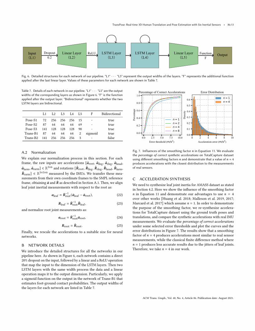
TransPose: Real-time 3D Human Translation and Pose Estimation with Six Inertial Sensors • 86:13
Fig. 6. Detailed structures for each network of our pipeline. "L1" · · · "L5" represent the output widths of the layers. "F" represents the additional functionapplied after the last linear layer. Values of these parameters for each network are shown in Table 7.
Table 7. Details of each network in our pipeline. "L1" · · · "L5" are the outputwidths of the corresponding layers as shown in Figure 6. "F" is the functionapplied after the output layer. "Bidirectional" represents whether the twoLSTM layers are bidirectional.
L1 L2 L3 L4 L5 F Bidirectional
Pose-S1 72 256 256 256 15 - truePose-S2 87 64 64 64 69 - truePose-S3 141 128 128 128 90 - trueTrans-B1 87 64 64 64 2 sigmoid trueTrans-B2 141 256 256 256 3 - false
A.2 NormalizationWe explain our normalization process in this section. For eachframe, the raw inputs are accelerations [�̃�root, �̃�lleg, �̃�rleg, �̃�head,�̃�larm, �̃�rarm] ∈ R3×6 and rotations [�̃�root, �̃�lleg, �̃�rleg, �̃�head, �̃�larm,�̃�rarm] ∈ R3×3×6 measured by the IMUs. We transfer these mea-surements from their own coordinate frames to the SMPL referenceframe, obtaining 𝒂 and �̄� as described in Section A.1. Then, we alignleaf joint inertial measurements with respect to the root as:
𝒂leaf = �̄�−1root (𝒂leaf − 𝒂root), (22)
𝑹leaf = �̄�−1root�̄�leaf , (23)
and normalize root joint measurements as:
𝒂root = �̄�−1root𝒂root, (24)
𝑹root = �̄�root . (25)
Finally, we rescale the accelerations to a suitable size for neuralnetworks.
B NETWORK DETAILSWe introduce the detailed structures for all the networks in ourpipeline here. As shown in Figure 6, each network contains a direct20% dropout on the input, followed by a linear and a ReLU operationthat map the input to the dimension of the LSTM layers. Then twoLSTM layers with the same width process the data and a linearoperation maps it to the output dimension. Particularly, we applya sigmoid function on the output in the network of Trans-B1 thatestimates foot-ground contact probabilities. The output widths ofthe layers for each network are listed in Table 7.
0.0 2.5 5.0 7.5 10.0Error threshold (m/s2)
0.0
0.2
0.4
0.6
0.8
1.0
Perc
enta
ge
Percentage of Correct Accelerations
n = 1n = 2n = 4n = 8
0 2 4 6 8 10Acceleration error (m/s2)
0.0
0.1
0.2
0.3
0.4
0.5
0.6
Den
sity
Error Distribution
n = 1n = 4
Fig. 7. Influences of the smoothing factor 𝑛 in Equation 11. We evaluatethe percentage of correct synthetic accelerations on TotalCapture datasetusing different smoothing factors 𝑛 and demonstrate that a value of 𝑛 = 4produces accelerations with the closest distribution to the measurementsof real sensors.
C ACCELERATION SYNTHESISWe need to synthesize leaf joint inertia for AMASS dataset as statedin Section 4.2. Here we show the influence of the smoothing factor𝑛 in Equation 11 and demonstrate our advantages to use 𝑛 = 4over other works [Huang et al. 2018; Malleson et al. 2019, 2017;Marcard et al. 2017] which assume 𝑛 = 1. In order to demonstratethe purpose of the smoothing factor, we re-synthesize accelera-tions for TotalCapture dataset using the ground truth poses andtranslations, and compare the synthetic accelerations with real IMUmeasurements. We evaluate the percentage of correct accelerationsunder some selected error thresholds and plot the curves and theerror distributions in Figure 7. The results show that a smoothingfactor of 𝑛 = 4 produces accelerations most similar to real sensormeasurements, while the classical finite difference method where𝑛 = 1 produces less accurate results due to the jitters of leaf joints.Therefore, we take 𝑛 = 4 in our work.
ACM Trans. Graph., Vol. 40, No. 4, Article 86. Publication date: August 2021.
![Matrix - University of Cambridge · transpose-matrix == Abs-matrix o transpose-infmatrix o Rep-matrix declare transpose-infmatrix-def [simp] lemma transpose-infmatrix-twice[simp]:](https://static.fdocuments.net/doc/165x107/5d5772d988c993f74a8b7fb4/matrix-university-of-cambridge-transpose-matrix-abs-matrix-o-transpose-infmatrix.jpg)


