TRANSPORT OF SOLUTES IN STREAMS WITH TRANSIENT...
171
Università degli Studi di Padova SCUOLA DI DOTTORATO DI RICERCA IN SCIENZE DELL’INGEGNERIA CIVILE E AMBIENTALE CICLO XXII Sede Amministrativa: Università degli Studi di Padova Dipartimento di Ingegneria Idraulica, Marittima, Ambientale e Geotecnica TRANSPORT OF SOLUTES IN STREAMS WITH TRANSIENT STORAGE AND HYPORHEIC EXCHANGE 31 Gennaio 2010 Direttore della Scuola: Ch.mo. Prof. Stefano Lanzoni Supervisore: Ch.mo. Prof. Andrea Marion Dottorando: Andrea Bottacin Busolin
-
Upload
truonglien -
Category
Documents
-
view
230 -
download
0
Transcript of TRANSPORT OF SOLUTES IN STREAMS WITH TRANSIENT...
Universitàdegli Studidi Padova
SCUOLA DI DOTTORATO DI RICERCA INSCIENZE DELL’INGEGNERIA CIVILE E AMBIENTALE
CICLO XXII
Sede Amministrativa: Università degli Studi di Padova
Dipartimento di Ingegneria Idraulica, Marittima, Ambientale e Geotecnica
TRANSPORT OF SOLUTES IN STREAMSWITH TRANSIENT STORAGE AND
HYPORHEIC EXCHANGE
31 Gennaio 2010
Direttore della Scuola: Ch.mo. Prof. Stefano Lanzoni
Supervisore: Ch.mo. Prof. Andrea Marion
Dottorando: Andrea Bottacin Busolin


Abstract
Environmental quality and health safety assessment often requires modeling of
solute transport in rivers. Conceptually, a stream can be divided into distinct
compartments mutually interacting through bidirectional exchanges of mass and
momentum. A distinction can generally be drawn between a main channel, whe-
re the velocities are relatively high, and different types of storage domains, where
the average velocity is sensibly lower. The downstream propagation of dissol-
ved substances in streams is influenced by exchanges between the main chan-
nel and surrounding retention zones, typically vegetated pockets, pools of re-
circulating or stagnant water, and permeable subsurface. Submerged vegetation
and, at a small spatial scale, microbial biofilms also constitute additional reten-
tion domains which can significantly contribute to determining the fate of the
transported substances.
A one-dimensional model for solute transport in rivers (STIR) with transient
storage is presented within this thesis. The model is based on a stochastic ap-
proach which allows to express the concentration of a solute in the main channel
of a stream as a function of the residence time distributions (RTDs) in the storage
domains. As a general RTD model, STIR can be used either as a calibration model
or as a predictive tool. When used as a calibration model, a form is assumed for
the RTD in the storage zones, and the relevant parameters are determined by fit-
ting the simulated breakthrough curves to concentration data from tracer tests.
On the other hand, if enough information is available about the properties of
I

Abstract
the system, specific modeling closures can be incorporated in STIR to represent
individual exchange processes separately.
In this work applications of the STIR model to field cases are presented whe-
re the model is calibrated with tracer test data. Distinct forms of the RTD in
the storage zones are assumed to assess the capability of the model to reprodu-
ce the observed tracer breakthrough curves. Results show that, when the RTD
in the storage zones is represented as a weighted average of two exponential di-
stributions, the model provides an excellent approximation of the experimental
data for all the study reaches examined and a useful conceptual separation of the
timescales of retention. However, since concentration distributions in streams re-
sult from a complex interaction between transport processes in the main channel
and exchange processes with the storage domains, uncertainty can arise about
the interpretation of the model parameters. The particular form assumed for the
storage time distribution determines the parameters of both surface transport
and transient storage. This limitation cannot be overcome with traditional field
tracer tests, unless complementing the experimental data with an accurate hydro-
dynamic modeling of the flow in the main channel. In flume experiments where
the hydraulic conditions can be strictly controlled, the effect of specific retention
processes can be isolated, under proper assumptions, by comparison of the mo-
del parameters with those relative to a reference configuration of the system in
which the retention processes under consideration are not present. This metho-
dology is illustrated with an application of STIR to data from flume experiments
with microbial biofilms.
Another important distinction often required in water quality assessments is
between in-channel and subsurface transient storage. The near-stream region of
the porous bed affected by the concentration of solutes in the stream is known
as the hyporheic zone, and is recognized to be extremely important for the evo-
lution of a riverine ecosystem. Exchange between the stream and the underlying
II

Abstract
hyporheic zone is known to be primarily driven by advective processes which de-
velop at several spatial scales because of separate mechanisms such as flow over
bed forms, around obstacles and through bars and meanders. Specific modeling
closures for the residence time distribution of bed form-induced hyporheic ex-
change are presented in this thesis for the case of homogeneous and stratified
beds, extending previous works on the subject. These modeling closures can
be incorporated in a general RTD transport model such as STIR to estimate in
a predictive manner the effect of bed form-induced hyporheic exchange on the
concentration of a solute in the surface water or, at least potentially, to estimate
particular parameters of hyporheic exchange with an inverse approach.
III

Sommario
La valutazione della qualità delle acque e le operazioni di monitoraggio ambien-
tale richiedono spesso la caratterizzazione dei processi di trasporto e ritenzione
di soluti nei sistemi fluviali. La propagazione a valle delle sostanze disciolte in un
corso d’acqua, come nutrienti e contaminanti, è influenzata da scambi di massa
tra corrente principale, dove le velocità sono relativamente elevate, e circostan-
ti zone d’immagazzinamento temporaneo, tipicamente zone vegetate, sacche di
ritenzione laterali e substrato permeabile, dove le velocità sono sensibilmente in-
feriori. Anche la vegetazione sommersa e, su piccola scala spaziale, i biofilm mi-
crobici costituiscono domini di ritenzione addizionali che possono condizionare
sensibilmente il destino delle sostanze trasportate.
Nel Capitolo 1 di questa tesi viene presentata una panoramica dei processi
di trasporto attivi nei corsi d’acqua su diverse scale spaziali e temporali, eviden-
ziando in particolare il loro contributo nell’equazione di bilancio di massa di un
soluto. Il Capitolo 2 offre una rassegna dei principali modelli monodimensionali
di trasporto ed immagazzinamento temporaneo proposti in letteratura. Nel Ca-
pitolo 3 viene presentato il modello di trasporto monodimensionale STIR (Solute
Transport In Rivers). Tale modello si basa su un approccio stocastico che permet-
te di esprimere la concentrazione di un soluto nel canale principale in funzione
della distribuzione del tempo di residenza nei domini d’immagazzinamento. La
formulazione a distribuzione generale del tempo di residenza rende STIR un mo-
dello flessibile e modulare che può essere usato sia come modello di calibrazione
V

Sommario
sia come strumento predittivo. Quando utilizzato come modello di calibrazione,
la stima dei parametri si basa su dati di concentrazione ottenuti mediante prove
con tracciante in sito. Si procede dunque assumendo una certa forma funziona-
le per la distribuzione del tempo di residenza nelle zone d’immagazzinamento
e determinando i relativi parametri in modo da minimizzare le differenze tra si-
mulazioni e dati sperimentali. Quando siano disponibili sufficienti informazioni
sulle proprietà di un corso d’acqua, specifiche chiusure modellistiche possono
essere incorporate nel modello STIR per rappresentare separatamente partico-
lari processi di ritenzione e valutare in modo predittivo la risposta del sistema
all’immissione di un soluto.
Nel Capitolo 4 viene presenta un’applicazione del modello STIR a prove con
tracciante in tre corsi d’acqua con caratteristiche molto diverse in termini di por-
tata, substrato e vegetazione. Distinte forme della distribuzione del tempo di
residenza nelle zone d’immagazzinamento sono assunte per valutare la capacità
del modello di riprodurre le curve osservate. I risultati mostrano che, quando
la distribuzione dei tempi d’immagazzinamento è espressa da una media pesata
di due distribuzioni esponenziali, il modello fornisce un’ottima approssimazio-
ne dei dati sperimentali in tutti i tratti di studio esaminati ed un’utile separa-
zione concettuale delle scale temporali caratteristiche dei processi di ritenzione.
L’interpretazione fisica dei parametri può tuttavia presentare delle incertezze,
in conseguenza del fatto che le distribuzioni di concentrazione nei corsi d’acqua
risultano da una complessa interazione tra processi di trasporto nella corrente
principale e processi di scambio con i domini di ritenzione. In particolare, se
i parametri del trasporto superficiale non sono fissati a priori, essi dipendono
dalla forma specifica assunta per la distribuzione dei tempi d’immagazzinamen-
to. Questa limitazione non può essere superata attraverso tradizionali prove con
tracciante, se non integrando i dati sperimentali con un’accurata modellazione
idrodinamica del corso d’acqua. Nel caso di prove con tracciante eseguite in ca-
VI

Sommario
naletta, dove le condizioni idrauliche sono in genere strettamente controllate,
l’effetto di particolari processi di ritenzione può essere isolato, sotto specifiche
assunzioni, prendendo come riferimento una configurazione di base del siste-
ma in cui tali processi non siano attivi. Questa metodologia viene illustrata nel
Capitolo 5 con un’applicazione del modello STIR volta a caratterizzare l’effetto
ritentivo di biofilm microbici mediante esperimenti in canaletta.
Negli studi di vulnerabilità di sistemi fluviali è utile distinguere tra proces-
si d’immagazzinamento superficiale e sotto-superficiale. Risulta importante, in
particolare, caratterizzare la ritenzione di soluti nella regione del letto, nota come
zona iporeica, che è direttamente influenzata dalla concentrazione nella corrente
superficiale. Essa costituisce infatti un importante ambiente di transizione e rive-
ste un ruolo fondamentale per l’evoluzione di un ecosistema fluviale. Lo scambio
tra la corrente e la sottostante zona iporeica è primariamente dovuto a processi
convettivi che si sviluppano su diverse scale spaziali a causa dell’interazione fra
corrente e irregolarità dell’alveo, quali forme di fondo, barre alternate e meandri.
Nei Capitoli 6 e 7 sono derivate specifiche chiusure modellistiche per lo scambio
iporeico indotto da forme di fondo in letti omogenei e stratificati che estendono
precedenti studi in materia. Tali chiusure modellistiche possono essere incorpo-
rate in un modello di trasporto come STIR per stimare in modo predittivo l’effetto
dello scambio iporeico indotto da forme di fondo sulla concentrazione di un so-
luto nell’acqua superficiale o, almeno potenzialmente, per stimare i parametri
dell’immagazzinamento iporeico mediante un approccio inverso.
VII

Contents
Abstract . . . . . . . . . . . . . . . . . . . . . . . . . . . . . . . . . . . . . . I
Sommario . . . . . . . . . . . . . . . . . . . . . . . . . . . . . . . . . . . . . V
1 Physical transport processes in fluvial environments . . . . . . . . . . 1
1.1 Advection . . . . . . . . . . . . . . . . . . . . . . . . . . . . . . . . . 1
1.2 Molecular diffusion . . . . . . . . . . . . . . . . . . . . . . . . . . . 3
1.3 Combined advection-diffusion processes . . . . . . . . . . . . . . . 4
1.4 Turbulent diffusion . . . . . . . . . . . . . . . . . . . . . . . . . . . 4
1.5 Dispersion . . . . . . . . . . . . . . . . . . . . . . . . . . . . . . . . 7
1.6 Transient storage . . . . . . . . . . . . . . . . . . . . . . . . . . . . . 8
2 Literature review of stream transport models . . . . . . . . . . . . . . 13
2.1 Introduction . . . . . . . . . . . . . . . . . . . . . . . . . . . . . . . 13
2.2 The Transient Storage Model (TSM) . . . . . . . . . . . . . . . . . . 14
2.3 The diffusive model . . . . . . . . . . . . . . . . . . . . . . . . . . . 16
2.4 The multi-rate mass transfer approach (MRMT) . . . . . . . . . . . 18
2.5 The continuous time random walk approach (CTRW) . . . . . . . . 20
2.6 Fractional advection-dispersion equation (FADE) . . . . . . . . . . 21
IX

Contents
3 The STIR model . . . . . . . . . . . . . . . . . . . . . . . . . . . . . . . . 25
3.1 Introduction . . . . . . . . . . . . . . . . . . . . . . . . . . . . . . . 25
3.2 The STIR model . . . . . . . . . . . . . . . . . . . . . . . . . . . . . 26
3.2.1 Residence times in the surface stream and in the storage
zones . . . . . . . . . . . . . . . . . . . . . . . . . . . . . . . 26
3.2.2 Uptake probability for uniformly spaced storage zones . . . 29
3.2.3 Example 1. Residence time distribution in surface dead
zones . . . . . . . . . . . . . . . . . . . . . . . . . . . . . . . 30
3.2.4 Example 2. Residence time distribution of bed form-induced
hyporheic retention . . . . . . . . . . . . . . . . . . . . . . . 30
3.2.5 Solute concentration in the surface stream and in the stor-
age domains . . . . . . . . . . . . . . . . . . . . . . . . . . . 31
3.3 STIR and other approaches . . . . . . . . . . . . . . . . . . . . . . . 35
3.4 Potential application . . . . . . . . . . . . . . . . . . . . . . . . . . 37
3.5 Conclusions . . . . . . . . . . . . . . . . . . . . . . . . . . . . . . . 39
4 Applications of the STIR model: Three case studies . . . . . . . . . . . 43
4.1 Introduction . . . . . . . . . . . . . . . . . . . . . . . . . . . . . . . 43
4.2 Site description . . . . . . . . . . . . . . . . . . . . . . . . . . . . . 45
4.2.1 The Yarqon river, Israel . . . . . . . . . . . . . . . . . . . . . 45
4.2.2 The Brenton torrent, Italy . . . . . . . . . . . . . . . . . . . 49
4.2.3 The Desturo canal, Italy . . . . . . . . . . . . . . . . . . . . 49
4.3 Stream tracer experiments . . . . . . . . . . . . . . . . . . . . . . . 51
4.4 Solute transport modeling . . . . . . . . . . . . . . . . . . . . . . . 57
4.5 Results and discussion . . . . . . . . . . . . . . . . . . . . . . . . . 60
4.6 Conclusions . . . . . . . . . . . . . . . . . . . . . . . . . . . . . . . 68
X

Contents
5 Effect of microbial biofilms on the transient storage of solutes . . . . 71
5.1 Introduction . . . . . . . . . . . . . . . . . . . . . . . . . . . . . . . 71
5.2 Experimental methods . . . . . . . . . . . . . . . . . . . . . . . . . 72
5.3 Solute transport modeling . . . . . . . . . . . . . . . . . . . . . . . 75
5.4 Model calibration . . . . . . . . . . . . . . . . . . . . . . . . . . . . 76
5.5 Results and discussion . . . . . . . . . . . . . . . . . . . . . . . . . 79
5.6 Conclusions . . . . . . . . . . . . . . . . . . . . . . . . . . . . . . . 87
6 Bed form-induced hyporheic exchange in homogeneous sediment beds 89
6.1 Introduction . . . . . . . . . . . . . . . . . . . . . . . . . . . . . . . 89
6.2 Solute transport model in the porous medium . . . . . . . . . . . . 91
6.2.1 Velocity field . . . . . . . . . . . . . . . . . . . . . . . . . . . 92
6.2.2 Advection-dispersion model . . . . . . . . . . . . . . . . . . 98
6.3 Residence time distributions . . . . . . . . . . . . . . . . . . . . . . 101
6.3.1 Pure advection . . . . . . . . . . . . . . . . . . . . . . . . . . 101
6.3.2 Effect of pore-scale dispersion . . . . . . . . . . . . . . . . . 106
6.4 Discussion . . . . . . . . . . . . . . . . . . . . . . . . . . . . . . . . 110
6.5 Conclusions . . . . . . . . . . . . . . . . . . . . . . . . . . . . . . . 114
7 Bed form-induced hyporheic exchange in stratified beds . . . . . . . . 117
7.1 Introduction . . . . . . . . . . . . . . . . . . . . . . . . . . . . . . . 117
7.2 Hyporheic flow modeling for layered beds . . . . . . . . . . . . . . 119
7.2.1 Velocity field in the bed . . . . . . . . . . . . . . . . . . . . . 119
7.2.2 Residence time distributions and mass exchange . . . . . . 123
7.3 Experiments . . . . . . . . . . . . . . . . . . . . . . . . . . . . . . . 125
7.3.1 Experimental setup . . . . . . . . . . . . . . . . . . . . . . . 125
7.3.2 Results . . . . . . . . . . . . . . . . . . . . . . . . . . . . . . 128
7.4 Comparison between model and experimental results . . . . . . . 130
7.5 Conclusions . . . . . . . . . . . . . . . . . . . . . . . . . . . . . . . 133
XI

Contents
Notation . . . . . . . . . . . . . . . . . . . . . . . . . . . . . . . . . . . . . . 135
Bibliography . . . . . . . . . . . . . . . . . . . . . . . . . . . . . . . . . . . . 143
XII

Chapter 1Physical transport processes in fluvial environments
Transport of dissolved substances in streams is determined at a small scale of ob-
servation by advection and molecular diffusion. When phenomena are observed
at a larger scale, thus considering quantities averaged in time and space, and
when the flow domain is conceptually divided into distinct compartments, for ex-
ample by separating surface from subsurface transport, additional processes be-
come apparent known as dispersion and transient storage. This chapter presents
an overview of how the physical transport processes active in fluvial environ-
ments are generally described at different spatial and temporal scales, highlight-
ing in particular their contribution to the mass balance equation.
1.1 Advection
Advection is the process by which a conserved physical quantity is transported in
a fluid in motion. In this work the transported quantity of interest is in particular
the mass of a dissolved substance. The amount per unit volume is expressed by
the concentration c [ML−3], while the motion of the fluid is entirely described by
the velocity vector field u = (u,v,w) [LT−1] defined at each point as a function of
time. If the substance behaves like a solute, that is, has the same density as the
medium or does not feel significant effect of its buoyant weight, each element of it
(molecule or particle) is displaced along the direction of the local velocity vector
1
1. Physical transport processes in fluvial environments
following the same path as if it were an element of the medium. This assumption
allows the advective transport to be modeled in a relatively simple way. The mass
flux Φ [ML−2 T−1] can be written as
Φ(x,t) = c(x, t)u(x, t) , (1.1)
where x = (x,y,z) is the coordinate vector in a Cartesian frame of reference and t
is time.
The mass balance for a control volume leads to the following differential equa-
tion:∂c∂t
= −∇ ·Φ , (1.2)
or, using the extended notation,
∂c∂t
= −∇ · (cv) = −[∂(cu)∂x
+∂(cv)∂y
+∂(cw)∂z
]. (1.3)
In fluvial hydraulics the fluid representing the medium in which substances are
dissolved is water, which can well be regarded as incompressible, and the flow
field is solenoidal (∇ · v ≡ 0). Under this assumption, the continuity equation
simplifies to∂c(x, t)∂t
+ u · ∇c(x, t) = 0 . (1.4)
In steady conditions, the solution of equation (1.4) is simply a translation of the
substance along the paths imposed by the flow field.
Pure advection does not exist alone in nature, as it is always associated at
least to molecular diffusion. However, the significance of molecular diffusion in
an advective process is negligible in most cases, due to the extremely low value
of the diffusive flux. Advection is associated only to molecular diffusion when
the flow field is slow, such as in laminar flows. One common application is the
2
1.2 Molecular diffusion
flow of water carrying substances in a porous medium, such as an aquifer or the
hyporheic zone, as long as the process is modeled at the scale of the pores of the
medium.
An important property of advection, valid also when diffusion is significant,
is that it determines the position of the center of mass of a solute cloud, thus
making the advection equation often sufficient to estimate the average travel time
of a solute between two subsequent positions in time.
The extension of the mass balance expressed by equation (1.4) to the trans-
port of buoyant or heavy substances is straightforward. This may be the case
of colloids or suspended solids which are affected by gravity as their density is
either smaller or larger than the density of the medium. Their behavior can be
modeled by adding a vertical velocity component with magnitude dependent on
the particle size, shape and density.
1.2 Molecular diffusion
Molecular diffusion is the process by which matter is transported from one part
of a system to another as a result of random molecular motions. A fundamental
property of this process is that the flux of mass is always directed from higher to
lower concentrations. A quantitative description of the diffusion process was first
given by Fick (1855) who expressed the corresponding net flux of the transported
substance as equal to the concentration gradient multiplied by a physical prop-
erty called molecular diffusivity or diffusion coefficient, indicated byDm [L2 T−1]:
Φ(x, t) = −Dm∇c(x, t) , (1.5)
where the symbol (∇) indicates the gradient differential operator.
When molecular diffusion is the only cause of mass transport, the mass bal-
3
1. Physical transport processes in fluvial environments
ance equation is given by Fick’s second law (or heat equation):
∂c(x, t)∂t
=Dm∇2c(x, t) =Dm
[∂2c(x, t)∂x2 +
∂2c(x, t)∂y2 +
∂2c(x, t)∂z2
]. (1.6)
The value of the molecular diffusion coefficient varies according to the combi-
nation of solute and solvent. As far as water is concerned, molecular diffusion is
easier for polar molecules andDm is of the order of 10−9÷10−8 m2 s−1. Conversely,
apolar molecules diffuse in water at lesser rate due to hydrophobic effects. The
molecular diffusion coefficient for these substances is of the order of 10−10 m2 s−1.
1.3 Combined advection-diffusion processes
Whenever the fluid is in motion, advection and diffusion processes act simulta-
neously. The total flux is thus given by the sum of the advective and diffusive
flux,
Φ = uc −Dm∇c , (1.7)
which leads to the following mass balance equation:
∂c∂t
= −∇ · (cu−Dm∇c) . (1.8)
For an incompressible fluid, equation (1.8) becomes
∂c∂t
+u∂c∂x
+ v∂c∂y
+w∂c∂z
=Dm
[∂2c
∂x2 +∂2c
∂y2 +∂2c
∂z2
]. (1.9)
1.4 Turbulent diffusion
Molecular diffusion produced by Brownian motion is no longer the dominant dif-
fusion mechanism when the flow velocity becomes fast enough to overcome vis-
cous forces that tend to keep fluid elements aligned along parallel paths. When
4

1.4 Turbulent diffusion
this condition is reached, the flowpaths become very irregular, and the fluid ele-
ments are entrained and transported by eddies which form either from the slow-
ing effect of the bottom and side boundaries or from the disturbances introduced
by geometrical irregularities. This type of flow is called turbulent, and is char-
acterized by an enhanced momentum and mass transfer across the flow field.
Diffusion of mass is no longer controlled by Brownian motion, but rather by the
continuous displacement of fluid elements in all directions induced by turbu-
lence. While molecular diffusion is isotropic, turbulent diffusion is typically dif-
ferent in each direction, as eddies are continuously stretched and deformed by
the flow.
Turbulent flows are usually modeled splitting the physical quantities into
time-averaged mean values and fluctuations around the mean. After manipu-
lation of the advection-diffusion equation (1.9), a new mathematical transport
term appears, which is the time-averaged product of the fluctuating values of ve-
locity and concentration. If velocity and concentration fluctuations were statisti-
cally independent, then these terms would produce no net diffusive mass fluxes.
It turns out instead that velocity and concentration irregularities are correlated
and that the integral effect over time of turbulent fluxes is always much higher
than the fluxes induced by Brownian motion. The time-averaged mass transport
equation becomes
∂c∂t
+u∂c∂x
+ v∂c∂y
+w∂c∂z
=∂∂x
(DTxx
∂c∂x
)+∂∂y
(DTyy
∂c∂y
)+∂∂z
(DTzz
∂c∂z
), (1.10)
where DTxx, DTyy and DTzz are eddy diffusion coefficients in the three spatial direc-
tions x, y and z, respectively, and the notation ( ) denotes temporal average. The
molecular diffusion coefficient Dm is typically so much smaller than eddy diffu-
sion coefficients that it can be neglected in the balance equation. A conceptual
difference between (1.10) and (1.9) is that the value of the coefficients DTxx, DTyy
5

1. Physical transport processes in fluvial environments
and DTzz is now determined by the flow regime, that is, they are flow properties,
while Dm is independent of the flow and determined only by the combination of
solute and solvent. Another difference resides in the fact that eddy diffusivity is
scale dependent, while molecular diffusivity is scale independent. Eddy diffu-
sivity typically scales with a 4/3 power of the length scale of the process. This
implies that as diffusion makes the substance spread in the domain, diffusivity
increases due to the effect of larger eddies that come into play. This dependence
is important in large and deep water bodies such as the sea or lakes, where the
diffusion process involves several different scales over time. In rivers, instead,
the size of the eddies is controlled by water depth and width, and diffusivity
is no longer affected by the scale of the process. An expression for the vertical
dispersion coefficient DTzz in rivers can be derived from the logarithmic velocity
profile:
DTzz = 0.067u∗dW , (1.11)
where dW is the water depth and u∗ is the shear velocity. An approximate expres-
sion of the coefficient DTyy valid for uniform straight channels was empirically
derived by Fischer et al. (1979) based on laboratory and field experiments:
DTyy = 0.15u∗dW . (1.12)
The typical irregularity of the cross-section in natural streams, characterized by
variations of both flow depth and width, enhances transverse mixing, and for
natural streams, Fischer et al. (1979) suggested the relationship
DTyy = 0.6u∗dW . (1.13)
For longitudinal mixing it can often be assumed that DTxx =DTyy .
These relationships can be used to estimate the distance Lmix from the injec-
6

1.5 Dispersion
tion point at which a solute can be considered to be well mixed over the cross-
section. For a solute injected in the middle of the channel section, Fischer et al.
(1979) suggested
Lmix = 0.1Ub2
DTxx, (1.14)
where U is the average flow velocity and b is the channel width. For a lateral
injection the distance is 4 times greater.
1.5 Dispersion
Dispersion is defined as the combined effect of advection and diffusion acting in
a flow field with velocity gradients. The effect of velocity gradients on the fate of
a substance becomes apparent when spatial averaging of the physical quantities
is carried out along with the temporal averaging described in § 1.4. In surface
water bodies, it is often convenient to simplify the description of mass transfer
by averaging velocity and concentration over the vertical direction (shallow wa-
ter approach) or over a cross-section (unidirectional approach). Depth averaging
is justified when dealing with large rivers, estuaries and lagoons, using the ev-
idence that vertical mixing is usually much faster than lateral and longitudinal
mixing, due to the limited extension of the domain in the vertical direction. The
one-dimensional approach is justified when the transverse dimensions of the do-
main are small compared to the longitudinal dimension. This is the reason why
the one-dimensional approach is commonly adopted for dispersion processes in
rivers and channels. In the case of cross-sectional averaging of the physical quan-
tities, the mass balance equation is reduced to the one-dimensional form:
∂C(x, t)∂t
+U (x, t)∂C(x, t)∂x
=1
A(x, t)∂∂x
(A(x, t)DL(x, t)
∂C(x, t)∂x
), (1.15)
where C and U are the cross-sectional average concentration and flow velocity,
respectively, A is the flow cross-sectional area [L2], and DL is the longitudinal
7

1. Physical transport processes in fluvial environments
dispersion coefficient [L2 T−1]. Under the assumption of constant A and DL, the
solution of equation (1.15) for an instantaneous injection of a mass of tracer M0
in x = 0 at time t = 0 is given by:
C(x, t) =M0/A√4πDLt
exp[−(x −Ut)2
4DLt
]. (1.16)
The presence of a nonuniform velocity distribution over the cross-section in-
duces solute molecules in different positions to travel different distances in a
given interval of time. On the other hand turbulent transverse mixing induces
the molecules to occupy different positions of the cross-section at subsequent in-
stants of time, thereby reducing the differences of travel distance among them.
Thus, the non-uniformity of the velocity distributions and turbulent transverse
mixing play a competitive role in determining the variance of the concentration
distributions. The longitudinal dispersion coefficient turns out to be proportional
to the spatial variability of the flow field around its mean value and inversely pro-
portional to the turbulent diffusivity. An approximated relationship for DL valid
for streams with large width-to-depth ratios was suggested by Fischer (1975) as
DL = 0.011U2b2
dWu∗, (1.17)
which has been found to agree to experimental observations within a factor of 4
or so.
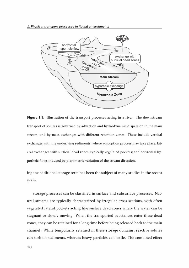
1.6 Transient storage
In natural streams, the downstream propagation of the transported substances
is influenced by mass exchanges with different types of storage zones, typically
vegetated pockets, dead zones and permeable subsurface, as illustrated in Fig-
ure 1.1. The superposition of retention phenomena acting at different timescales
induces a non-Fickian behavior of the observed breakthrough curves that cannot
8

1.6 Transient storage
be reproduced using the classical advection-dispersion equation (1.15). This lim-
itation has been proved since the early 50’s by a number of studies using tracer
tests (Elder, 1959; Krenkel and Orlob, 1962; Thackston and Schnelle, 1970; Nordin
and Sabol, 1974; Day, 1975; Nordin and Troutman, 1980). The effect of retention
phenomena on the concentration distributions can be summarized as follows:
• The skewness of the observed breakthrough curves is more pronounced
than predicted by the advection-dispersion theory, and the curves are char-
acterized by longer tails.
• The variance of the concentration distributions increases more than linearly
in time.
• The concentration peak decreases more rapidly than the −1/2 power of
time.
• The concentration peak moves at a lower speed than the average flow ve-
locity.
• Part of the solute is not recovered at the measurement section, especially
when solutes reacts with sediments, such as metals, or when the trans-
ported substances are affected by gravity.
In order to account for the temporary storage of solutes, the advection-disper-
sion equation (1.15) can be modified by including in the mass balance an addi-
tional flux due to mass exchange between the flow in the main channel and the
surrounding storage zones. The equation then becomes:
∂C∂t
+U∂C∂x
=1A∂∂x
(ADL
∂C∂x
)− PAΦS , (1.18)
whereΦS denotes the exchange flux at the stream-storage zone interface [ML−2 T−1].
The physical description and the modeling of the retention processes determin-
9
1. Physical transport processes in fluvial environments
Figure 1.1. Illustration of the transport processes acting in a river. The downstream
transport of solutes is governed by advection and hydrodynamic dispersion in the main
stream, and by mass exchanges with different retention zones. These include vertical
exchanges with the underlying sediments, where adsorption process may take place; lat-
eral exchanges with surficial dead zones, typically vegetated pockets; and horizontal hy-
porheic flows induced by planimetric variation of the stream direction.
ing the additional storage term has been the subject of many studies in the recent
years.
Storage processes can be classified in surface and subsurface processes. Nat-
ural streams are typically characterized by irregular cross-sections, with often
vegetated lateral pockets acting like surface dead zones where the water can be
stagnant or slowly moving. When the transported substances enter these dead
zones, they can be retained for a long time before being released back to the main
channel. While temporarily retained in these storage domains, reactive solutes
can sorb on sediments, whereas heavy particles can settle. The combined effect
10
1.6 Transient storage
of deposition of heavy particles and adsorption of reactive solutes is particularly
important: the formers in fact can become the substrate on which reactive solutes
adsorb. Deposition and adsorption can cause a temporary or persistent mass loss,
and influence significantly contamination processes in streams and rivers.
Subsurface storage processes result from exchange fluxes between the stream
and the sediment bed over which water flows. Filtration through porous bound-
ary of a river bed leads the dissolved substances within the porous medium where
sorption onto the sediments, deposition of the finer suspended particulate matter
and other biogeochemical reactions may significantly affect their fate. The near-
stream region of the porous boundary affected by the concentration of solutes
in the stream is called the hyporheic zone, and is recognized to be an important
transition environment for the evolution of a riverine ecosystem.
11


Chapter 2Literature review of stream transport models
2.1 Introduction
Hydrodynamic exchange with storage zones plays an important role in determin-
ing the fate of the transported substances in streams. The effect of transient stor-
age is often clearly visible in the shape of breakthrough curves of stream tracer
tests, which cannot be reproduced by the conventional ADE, especially when the
timescales of retention are much larger than the travel time in the main channel.
Long term retention processes are typically due to the temporary storage in the
porous medium, in the so called hyporheic zones, while short term retention is
commonly due to surface dead zones, such as side pockets of recirculating water
or vegetated zones. The prediction of the exchange between a stream and the
surrounding retention zones is an important component in the analysis of the
contamination dynamics of fluvial environments. Retention processes in the hy-
porheic zones can be studied individually with mathematical or numerical mod-
els by simulating the transport dynamics of a solute in a sediment bed. This is
usually done for idealized configurations by decoupling surface from subsurface
flow. In the experimental approach relying on tracer tests, hyporheic retention
is instead studied from the perspective of the surface transport, by evaluating
its effect as a whole on the concentration of a solute in the surface water. This
13

2. Literature review of stream transport models
approach is typically based on one-dimensional transport models consisting in
properly modified advection-dispersion equations. A brief review of the main 1-
D transport models proposed in the literature is given in the following sections.
2.2 The Transient Storage Model (TSM)
One of the most widely used transport models in field applications reported in
the literature is the Transient Storage Model (TSM). The TSM was presented by
Bencala and Walters (1983), although analogous formulations can be found in an
earlier works (Hays et al., 1966; Nordin and Troutman, 1980). This model has
been widely applied to field experiments conducted both in small streams and
large rivers (e.g. Bencala, 1984; Castro and Hornberger, 1991; Vallet et al., 1996;
Mulholland et al., 1997a; Harvey and Fuller, 1998; Runkel et al., 1998; Choi et al.,
1999; Fernald et al., 2001).
In the TSM the net mass transfer from the main flow channel to the reten-
tion domains is assumed to be proportional to the difference of concentration be-
tween the surface water and a storage zone of constant cross-sectional area. The
mathematical formulation of the TSM for non-reactive solutes is usually given as
follows (Nordin and Troutman, 1980; Bencala and Walters, 1983; Czernuszenko and
Rowinski, 1997; Lees et al., 2000; De Smedt and Wierenga, 2005; De Smedt, 2006):
∂CW∂t
+U∂CW∂x
=DL∂2C
∂x2 +α(CS −CW ) , (2.1a)
dCSdt
= −α AAS
(CS −CW ) , (2.1b)
where: U is the mean flow velocity [LT−1]; α is a transfer coefficient [T−1]; A/AS
is the ratio of stream to storage cross-sectional areas; CW is the in-stream so-
lute concentration [ML−3]; CS is the concentration of solute in the storage zone
[ML−3]; DL is the longitudinal dispersion coefficient for the flow in the main
channel [L2 T−1]; and t is time [T]. A numerical solution of equation (2.1) was
14
2.2 The Transient Storage Model (TSM)
presented by Runkel and Chapra (1993), which formed the basis of their One-
dimensional Transport with Inflow and Storage (OTIS), later extended by Runkel
(1998) with a parameter estimation technique (OTIS-P).
Equation (2.1a) is a special case of (1.18) where the exchange flux is assumed
to be equal to:
ΦS =APα(CW −CS) . (2.2)
Often an additional flux, ΦL, is included in the mass balance to account for pos-
sible mass gains due to lateral inflow. This is defined as
ΦL = qL(CW −CS) , (2.3)
where qL is the volumetric flux [LT−1] and CL is the concentration of solute in
lateral inflow.
Equation (2.1b) can be solved to get CS as a function of CW :
CS(x, t) = αAAS
∫ t
0CW (x, t − τ)e−
αAASτdτ , (2.4)
which shows that the TSM implies an exponential residence time distribution
(RTD) in the storage zones with mean value T = AS /(αA).
The particular form of the model given by equation (2.1) finds application to
passive, conservative tracers, that is, non-reactive substances which do not decay
over time. These effects can be accounted for by including in (2.1) a kinetic term
as suggested by Bencala and Walters (1983). An extension of the model to account
for reactivity of solutes was proposed by Runkel et al. (1996) who coupled the
TSM with a submodel for equilibrium adsorption and other phenomena such as
precipitation related to water pH values.
The parameters of the TSM are usually determined by fitting the model simu-
lations to experimental breakthrough curves obtained by tracer tests. The intro-
15

2. Literature review of stream transport models
duction of an additional flux in the mass balance allows a better representation of
the breakthrough curves observed in natural streams. However, since the param-
eters can be determined only by calibration, they do not necessarily have physical
meaning, because they are not directly related to the real dynamics of the phys-
ical processes generating transient storage. There is no theory that provides a
relationship between the transfer rate α and the area AS to measurable physical
quantities of the system examined. This means that the results found in the ap-
plication of the TSM to a particular system cannot be extended to another one
with different characteristics.
The simplification of the physical processes involved in hyporheic exchange
which is inherent in the TSM is a cause of uncertainty in the parameter estima-
tion. Recent studies and field observations have demonstrated that when advec-
tive pumping into the bed is a significant exchange process the best fit TSM pa-
rameters are dependent on the timescale of the process and the upstream bound-
ary condition (incoming concentration) (Harvey et al., 1996; Harvey and Wagner,
2000; Wörman et al., 2002; Marion et al., 2003; Zaramella et al., 2003; Marion and
Zaramella, 2005a). This uncertainty of the TSM parameters often interferes with
the observation of important results, such as the relationship between transient
storage and the fluxes of reactive substances of interest (e.g., nutrients, contam-
inants) (Hall Jr. et al., 2002; Zaramella et al., 2006). From this consideration the
need arises to extend transport models to account for specific retention processes
that can be studied and modeled separately as a function of measurable physical
quantities characterizing the system.
2.3 The diffusive model
A model for solute transport of conservative species where hyporheic exchange
is represented by a diffusive term was suggested by Jackman et al. (1984). This
model assumes solute penetration into the bed to be a vertical diffusion process
16
2.3 The diffusive model
described by Fick’s law. The equation governing the transport of a solute in the
bed is therefore given by:∂CS∂t
=DS∂2CS∂y2 , (2.5)
where CS(t,x,y) and DS are respectively the concentration and the dispersion
coefficient in the porous medium. In the general equation (1.18), the flux at the
stream-subsurface interface is assumed to be proportional to the local gradient
of concentration in the bed:
ΦS(t,x) = −DS∂CS(t,x,y)
∂y
∣∣∣∣∣y=0
, (2.6)
where DS is the diffusion coefficient in the porous medium. The boundary condi-
tion in y = 0 for equation (2.5) is given by CS = CW , whereas the initial condition
is usually assumed to be CS(t = 0,x,y) = 0. Assuming y positive downward, the
solution of equation (2.5) for the given boundary and initial conditions is
CS(t,x,y) =y
2√πDS
∫ t
0CW (τ,x) exp
[−
y2
4DS(t − τ)
]dτ
(t − τ)3/2, (2.7)
and hence, from (2.6) we get
ΦS(t,x) =12
√DSπ
∫ t
0
CW (τ,x)(t − τ)3/2
dτ . (2.8)
The coupling of the advection-dispersion model for the surface flow and the ver-
tical diffusion model for the subsurface yields:
∂CW∂t
+U∂CW∂x
=1A∂∂x
(ADL
∂CW∂x
)− PA
√DS4π
∫ t
0
CW (τ,x)(t − τ)3/2
dτ . (2.9)
It should be noted that the transfer mechanism assumed in the diffusive model is
not reversible as in the TSM. In the TSM the fraction of solute entering the stor-
17
2. Literature review of stream transport models
age domains is gradually released when the concentration in the surface water
becomes lower than the concentration in the storage zone, whereas in the diffu-
sive model the mass transfer is one-directional and the exchange with the bed
generates a net mass loss of solute in the surface water.
2.4 The multi-rate mass transfer approach (MRMT)
In the MRMT formulation the flow domain is divided in mobile and immobile
regions. In the mobile regions solute transport is modeled by the classical ADE,
while immobile regions cause local interaction that retard tracer migration. In
streams, the mobile domain is given by the main channel, while the storage zones
represent the immobile regions. In the one-dimensional case, the migration of
a solute along the mobile domain is described by the following mass balance
equation (Haggerty et al., 2000)
∂CW∂t
+ ΓS(x, t) =∂∂x
(DL∂CW∂x−UCW
), (2.10)
where ΓS(x, t) [ML−3 T−1] is the source-sink term for the mass exchange with
the immobile sites and it is commonly assumed to be independent of x. Equa-
tion (2.10) is essentially the same as (1.18) with ΓS(x, t) = −P /AΦS(x, t).
The source-sink term ΓS(t) can be expressed as a derivative of the concentra-
tions in the immobile domains (van Genuchten and Wierenga, 1976), but it is often
more convenient to express it as a convolution integral, following Carrera et al.
(1998). This is given by:
ΓS(t) =∫ t
0
∂CW (x, t − τ)∂τ
fM(τ)dτ =∂CW (x, t)
∂t∗ fM(t)
= CW ∗∂fM(t)∂t
+CW (x, t)fM(0)−CW (x,0)fM(t) ,
(2.11)
18

2.4 The multi-rate mass transfer approach (MRMT)
where the asterisk denote convolution product, and fM(t) is a memory function
[T−1]. A general form of the memory function can be given as (Haggerty et al.,
2000; Carrera et al., 1998)
fM(t) =∫ ∞
0αpα(α)e−αt dα , (2.12)
where α is a rate coefficient [T−1] and pα(α) is a probability density function of
first-order coefficients [T].
Haggerty et al. (2000) presented a number of possible forms for the density
pα(α). Among these, the truncated power law density has received particular
attention in the last decade:
pα(α) =βtot(κ − 2)
ακ−2max −ακ−2
min
αk−3 , κ > 0 , k , 2 , αmin ≤ α ≤ αmax , (2.13)
where αmax [T−1] is the maximum rate coefficient, αmin [T−1] is the minimum rate
coefficient, and κ is the exponent, and βtot is the capacity coefficient (Haggerty
and Gorelick, 1995). The capacity coefficient is the zeroth moment of the density
function of rate coefficients,
βtot =∫ ∞
0pα(α)dα , (2.14)
and turns out to be the ratio of mass in the immobile domain to mass in the
mobile domain at equilibrium, or simply the ratio of the two volumes in absence
of sorption (Haggerty et al., 2000). The memory function fM(t) is given by
fM(t) = βtot
∫ αmax
αmin
(k − 2)αk−2e−αt
αk−2max −αk−2
min
dα . (2.15)
This is a summation of exponential distributions with a power-law weighting
function. The resulting memory function scales as fM ∼ t1−k between the times
19
2. Literature review of stream transport models
α−1max and α−1
min. Equation (2.10) combined with the memory function given by
(2.15) has been found to provide good approximation of experimental tracer
breakthrough curves in a few cased studies (Haggerty and Wondzell, 2002; Gooseff
et al., 2003b, 2007).
2.5 The continuous time random walk approach (CTRW)
In the conceptual framework of the continuous time random walk (Montroll and
Weiss, 1965; Scher and Lax, 1973), the motion of solute molecules (or “particles”)
is envisioned as a sequence of displacements (or “jumps”) of variable length and
duration considered as random variables. In this framework, the concentration
of a solute at a given instant and position is derived statistically as the probability
for a particle to occupy the specified position at the specified time. The classical
advection-dispersion equation (ADE) can be derived as a special case of a con-
tinuous time random walk in which every displacement has the same length and
occurs in random directions at regular time intervals (e.g. Fischer et al., 1979). In
the CTRW theory the length and duration of particle jumps are random variables
with joint probability density function (PDF) Ψ (x, t), and marginal distributions
ψL(x) and ψT (t), respectively. This conceptualization of particle motion leads to
the following generalized master equation (GME) :
∂C(x, t)∂t
= −∫ t
0fM(t − τ)
[U∂C(x,τ)∂x
−DL∂2C(x,τ)∂x2
]dτ , (2.16)
where
U = 1t
∫ +∞−∞ xψL(x)dx , (2.17)
DL = 12t
∫ +∞−∞ x2ψL(x)dx , (2.18)
are the time-invariant velocity and longitudinal dispersion coefficient, respec-
tively, over the averaging timescale t. The function fM(t) in equation (2.16) is a
20

2.6 Fractional advection-dispersion equation (FADE)
memory function defined in the Laplace domain as
f̃M(s) = stψ̃T (s)
1− ψ̃T (s), (2.19)
where the symbol (̃ ) denotes Laplace transform,
f̃M(s) =∫ ∞
0fM(t)e−st dt , (2.20)
and s is the Laplace variable.
The structure of the GME (2.16) is analogous to the ADE, but with the ad-
dition of a convolution integral with the memory function fM(t). This memory
function depends uniquely on the marginal distribution of the jump duration,
ψT (t), while the parameters U and DL are given respectively by the first and sec-
ond moment of the length PDF ψL(x). The presence of a convolution integral
implies that the equation is, in general, nonlocal in time. As a special case, the
GME reduces to the conventional ADE when ψT (t) is an exponential PDF, which
implies that fM(t) is a Dirac delta function, fM(t) = δ(t). By providing a suitable
expression of ψT (t), the GME can be used to describe the typical non-Fickian
behavior of the observed tracer breakthrough curves. The CTRW approach has
been widely applied to study anomalous dispersion in fractured and heteroge-
neous media (e.g. Berkowitz and Scher, 1995; Scher et al., 2002), and has recently
been applied to the transport of solutes in streams (Boano et al., 2007).
2.6 Fractional advection-dispersion equation (FADE)
A generalization of the classical advection-dispersion equation can be given using
mathematical tools of fractional calculus. The right and left derivative of order ε
21
2. Literature review of stream transport models
can be defined respectively as (Samko et al., 1993):
∂ε+xC(x, t) =1
Γ (n− ε)dn
dxn
∫ x
−∞(x − ξ)n−ε−1C(ξ, t)dξ , (2.21a)
∂ε−xC(x, t) =(−1)n
Γ (n− ε)dn
dxn
∫ ∞x
(ξ − x)n−ε−1C(ξ, t)dξ , (2.21b)
where n is the minimum integer greater than or equal to ε and
Γ (x) =∫ ∞
0ξx−1e−ξdξ (2.22)
is the gamma function. While the integer derivative provides information about
the local function behavior, the fractional derivative provides information about
the whole function Blank (1996). The fractional derivative operator can be said to
be the weighted averaging operator of the entire function at a certain point, and
the fractional order is linked to the spatial correlation length of the embedding
system (Kim and Kavvas, 2006).
Using fractional order derivatives, Fick’s law can be generalized to the form
(Chaves, 1998; Metzler and Klafter, 2000; Schumer et al., 2001)
Φ = −Dε(1 + ς
2∂ε−1
+x +1− ς
2∂ε−1−x
)C +UC , 0 < ε ≤ 1 , (2.23)
where Dε is a dispersion coefficient and −1 ≤ ς ≤ 1 is a skewness parameter.
For ε = 1 and ς = 0 (2.23) reduces to the classical Fick’s law. Combining equa-
tion (2.23) with the continuity equation, the fractional advection-dispersion equa-
tion is obtained:
∂C∂t
+U∂C∂x
=Dε(1 + ς
2∂ε+x +
1− ς2
∂ε−x
)C . (2.24)
In writing (2.24) the flow cross sectional area A and the dispersion coefficient
Dε were assumed to be independent of x. The solution of equation (2.24) for
22

2.6 Fractional advection-dispersion equation (FADE)
an impulsive injection of a mass of tracer M0, that is C(x,0) = M0/Aδ(x), can be
derived using the Fourier transform and is given by
C(x, t) =1
4π2M0
A
∫ ∞−∞p(k, t)eik(x−Ut)dk , (2.25)
where i is the immaginary unit, k is the wavenumber [L−1] and p(k, t) is a function
is defined as
p(k, t) = exp[|kε|Dε cos
(επ2
)t]× exp
[i|kε|ςDε sin
(επ2
)t]. (2.26)
This can be shown to be the characteristic function of a Levy distribution.
Depending on the parameters ε, ς and Dε, the residence time distributions
predicted by the fractional advection-dispersion equation can be sensibly skewed
and heavy tailed resembling those typically observed in natural streams. Appli-
cations of the fractional ADE has been reported by Deng et al. (2004) and Deng
et al. (2006) showing good agreement with experimental data. The main limita-
tion of the fractional approach is that the real physics of the transport processes
involved is hidden in a complex mathematical formalism making the parameters
difficult to interpret.
23


Chapter 3The STIR model1
3.1 Introduction
The models presented in the previous chapter provide a mathematical descrip-
tion of how the concentration of a solute transported in a stream is affected by
retention processes. Among these, the MRMT and the CTRW approach enable
general residence time distribution (RTD) modeling, which is a particularly flex-
ible way to represent retention phenomena in streams. This chapter presents an
alternative conceptual model (STIR) that provides a physically based description
of the stream-storage zone interactions on river mixing. A first simpler version
of the STIR model was presented by Marion and Zaramella (2005b) as a multiple
process extension of the single process stochastic model proposed by Hart (1995).
Here, the STIR model is presented in a comprehensive mathematical framework
that extends the original formulation. It is shown that, under specific assump-
tions, STIR converges to other models, such as the TSM, the Multirate Mass Trans-
fer (MRMT) and the CTRW approach. For practical applications STIR can be seen
as an extension of Transient Storage Model (TSM) in which general forms of the
1The contents of this chapter have been published in: Marion, A., M. Zaramella, and
A. Bottacin-Busolin (2008), Solute transport in rivers with multiple storage zones: The STIR
model, Water Resour. Res., 44, W10406.
25
3. The STIR model
storage time statistics can be implemented. The capability of the model is illus-
trated with a theoretical example. Further applications of the model to tracer test
data from both natural streams and flume experiments will be presented in the
next chapters.
3.2 The STIR model
The development of a model that mimics the longitudinal dispersion of a solute
in a river, coupled with transient storage, requires the schematization of the sys-
tem and an adequate degree of synthesis of the physics governing the processes.
The stream is modeled as a one-dimensional system where x is the longitudinal
distance, A is the cross-sectional area, U is the mean stream velocity and DL is
the longitudinal dispersion coefficient. It must be stressed that, in this concep-
tual framework, DL accounts only for the effect of the surface flow field, and does
not coincide with the “comprehensive” longitudinal dispersion coefficient often
used to lump transient storage into the mass balance equation. Since the goal
of this modeling approach is to separate the processes, the river is represented
as a system composed by distinct physical domains interacting with each other
through mass exchanges. The river is divided into the surficial stream in the main
channel and different retention domains, such as surficial dead zones and the hy-
porheic layer. The downstream transport of solutes is assumed to be controlled
by exchanges with N types of storage zones, each one characterized by a given
residence time distribution.
3.2.1 Residence times in the surface stream and in the storage zones
The propagation of a solute along a river is treated as a stochastic process. The
time needed for a particle to travel a distance x, indicated with T , is a random
variable with probability density function r(t;x). The time T is the sum of a
time TW spent on the surface, with PDF rW (t;x), and a time TS sum of the sin-
gle residence times within the storage domains, TS =∑Ni=1TSi . A particle moving
26
3.2 The STIR model
from the main stream into a storage zone follows a certain path and may possi-
bly return back to the main stream after some time. Particles may be uptaken
once, twice or more, resulting in a global behavior that is the sum of individ-
ual paths partly in the main surface flow, partly in the retention domains. It is
assumed that the longitudinal displacements within the storage zones are negli-
gible compared to the displacement in the surface water. The number of times a
particle is trapped in the i-th retention domain,Ni , is a discrete random variable
(Ni = 0,1,2 . . .) with conditional distribution pi(n|TW = tW ). When a particle is
trapped in a storage zone, it is released after a time with PDF ϕi(t). Since the
trapping events are assumed independent, the time TSi has conditional density
rSi|n(t) = ϕi(t) ∗ . . .∗︸︷︷︸n times
ϕi(t) = [ϕi(t)]∗n , (3.1)
given Ni = n. Here the symbol (∗) denotes time convolution, so that ϕ(t) ∗ϕ(t) =∫ t0ϕ(τ)ϕ(t − τ)dτ , where τ is a dummy variable. When n = 0, equation equa-
tion (3.1) yields rSi|0(t) = δ(t), where δ(t) is the Dirac delta function (s−1). It fol-
lows that the conditional density of TSi given TW = tW is
rSi(t|tW ) =∞∑n=0
pi(n|tW )rSi|n(t) . (3.2)
When the transport process is dominated by advection, the uptake probability, pi ,
can also be thought as a function of the travel distance, x, which is proportional
to the mean time spent on the surface. The condition of dominant-advection is
generally given as (Rutherford, 1994)
xU� DLU2 , (3.3)
27

3. The STIR model
which is satisfied in most practical applications in rivers. The spatial dependence
could also be more appropriate when there is a low density of retention zones.
The probability of a particle to be uptaken at a given instant is assumed to be
unconditioned by its previous storage history, then TSi , i = 1, . . . ,N , are mutually
independent, and the conditional density of TS given TW = tW is
rS(t|tW ) = rS1(t|tW ) ∗ . . . ∗ rSN (t|tW ) . (3.4)
A particle moving along the stream follows an irregular path due to turbu-
lence. Following well established results from the literature (Taylor, 1954; Elder,
1959; Fischer, 1968), the motion of a particle limited only to surface flow in the
main channel can be described as equivalent to a Brownian motion with drift, and
the relevant residence time distribution can be inferred from the solution of the
advection-dispersion equation (ADE). If it is now assumed that the entrapment
within the storage zones does not modify the particle pathways, then the resi-
dence time within the surface stream remains unaltered. Thus, when the compu-
tational domain is x > 0, with boundary condition at infinity C(x→∞, t) = 0, the
function rW (t;x) is given by:
rW (t;x) =x
2√πDLt3
exp[−(x −Ut)2
4DLt
]. (3.5)
Equation equation (3.5) is derived from the solution of the ADE for an input mass
pulse, UC −DL∂xC =M0/Aδ(t) at x = 0, where M0 is the injected mass.
It is now possible to express the overall residence time distribution within a
stream reach of length x as
r(t;x) =∫ t
0rW (t − τ ;x)rS(τ |t − τ)dτ . (3.6)
Alternatively, when the total storage time is assumed to be dependent on the
28
3.2 The STIR model
travel distance, thus using rS(t;x) instead of rS(t|tW ), the overall RTD is given by:
r(t;x) = rW (t;x) ∗ rS(t;x) . (3.7)
3.2.2 Uptake probability for uniformly spaced storage zones
Under the assumption of uniform distribution of storage zones along the river,
the uptake probability can be expressed as follows. The probability for a particle
in the surficial stream to be stored in the i-th domain in a time interval δt is
assumed to be proportional to the length of the interval. It is expressed as αiδt,
where αi [T−1] is the probability per unit time, which is taken to be constant both
in time and space (although the temporal constance is not strictly required). The
quantities αi represent the rates of transfer or, in other words, the flow rate into
the storage zones per unit surficial volume. When hyporheic exchange with the
stream bed is considered, the relevant rate αB can be expressed as
αB =qBdW
, (3.8)
where qB is the average flow rate into the sediments per unit bed area [LT−1], and
dW is the flow depth [L].
Since the probability for a particle to be caught in the i-th storage zone at a
given instant is independent from its previous history, the probability for a parti-
cle to be caught n times in a time interval tW is given by the Poisson distribution
with parameter αitW :
pi(n|tW ) =(αitW )n
n!e−αitW . (3.9)
Alternatively, the uptake probability can be thought as a function of the distance
from the injection point, x0 = 0, thus
pi(n;x) =(αix/U )n
n!e−αix/U . (3.10)
29

3. The STIR model
It is finally noted that, when equation equation (3.9) is used for the uptake
probability, the Laplace Transform (LT) of the overall residence time distribution
expressed by equation equation (3.6) can be arranged, after some mathematical
manipulations, in the following form (Margolin et al., 2003):
r̃(s;x) =∫ ∞
0r(t;x)e−st dt = r̃W
s+N∑i=1
αi(1− ϕ̃i(s)); x
, (3.11)
where the symbol (̃ ) denotes Laplace Transform of the function it is applied to.
Equation equation (3.11) shows that in Laplace domain the resulting residence
time PDF is the same found in the absence of any retention process, but with a
frequency shift that depends on the storage time PDFs.
3.2.3 Example 1. Residence time distribution in surface dead zones
The exchange with surface dead zones of finite volume is well represented by an
exponential RTD. The expression of the single-uptake storage time PDF is then
the following
ϕD(t) = 1TDe−t/TD , (3.12)
where TD is a time scale, equal to the mean residence time. In practice the effect
of the surface dead zone retention usually acts in a relatively short time scale
compared to hyporheic retention, and can often be measured by tracer tests.
3.2.4 Example 2. Residence time distribution of bed form-induced hyporheic
retention
Hyporheic flows are hardly measurable by direct methods, such as tracer tests,
unless very long and very expensive techniques are designed (Johansson et al.,
2001; Wörman et al., 2002; Gooseff et al., 2003a; Jonsson et al., 2003, 2004). The
Advective Pumping Model (APM) (Elliott and Brooks, 1997a) provides an expres-
sion for the cumulative residence time function within the sediments for bed
30

3.2 The STIR model
form-induced exchange. Elliott’s solution was given in term of an implicit func-
tion of time, whereas the application of equations equation (3.6), equation (3.7)
and equation (3.11) requires an explicit form of the PDF of the residence time
within the sediments ϕB(t). An analytical expression of ϕB(t) that approximates
the exact solution for the case of the bed form-induced exchange is (Marion and
Zaramella, 2005b):
ϕB(t) =π/TB
βTBt +
(t
TB+ 2
)2 , (3.13)
where the parameter β satisfies the following equation:
∫ ∞0ϕB(t)dt =
∫ ∞0
π/TB
βTB/t + (t/TB + 2)2dt = 1 . (3.14)
Equation equation (3.14) is a necessary condition to make ϕB(t) a PDF and is
satisfied by β = 10.66. Parameter TB represents a residence timescale in the sub-
surface. The proposed residence time PDF is a single parameter heavy-tailed
distribution that, for t → ∞, decays as a power law, ϕB(t) ∼ πTBt−2. Compar-
ison between the exact and the approximate expression of ϕB(t) is reported in
Figure 3.1.
3.2.5 Solute concentration in the surface stream and in the storage domains
In this section, a relationship between the in-stream solute concentration and the
residence time distribution is derived.
Consider a stream reach of length x in which a mass M0 is instantaneously
injected at the upstream section, x0 = 0, at time t0 = 0. At any instant t > 0, a part
of the total mass is distributed in the main surficial stream, while a part is tem-
porarily retained within the storage domains. The relevant masses are indicated
by MW and MS , respectively. The total concentration is then defined as:
C(x, t) = limδx→0
δMW (x, t) + δMS(x, t)Aδx
= CW (x, t) + limδx→0
δMS(x, t)Aδx
, (3.15)
31

3. The STIR model
0
0.04
0.08
0.12
0.16
0.01 0.1 1 10010
Exact (APM)Approximate
t B
()t
BB
Figure 3.1. Comparison between the exact and the approximate PDF of the residence
time within the sediment. The gap between the two curves is visible only at early times
and is negligible for practical applications.
where δMW (x, t) and δMS(x, t) are the masses contained within the spatial inter-
val [x,x + δx] at time t in the superficial stream and in the storage zones, respec-
tively.
The quantity r(t;x)dt represents the fraction of mass flowing through the
downstream section in the time interval [t, t + dt], and the flux is given by the
convolution of r(t;x) with the input flux φ0(t). For a mass pulse concentrated
in time this is given by φ0(t) = M0/Aδ(t). The variation per unit time of the
total concentration is equal to the opposite of the divergence of the local flux,
φ0(t) ∗ r(t;x), hence
∂Cδ(x, t)∂t
= − ∂∂x
∫ t
0φ0(τ)r(t − τ ;x)dτ = −M0
A
∂r(t;x)∂x
, (3.16)
where the subscript δ is used to denote the solute concentration generated by a
mass pulse. The difference between the input and the output flux at the stream-
32
3.2 The STIR model
storage zone interface is linked to the variation of C −CW according to:
∂(C −CW )∂t
=N∑i=1
(αiCW (x, t)−
∫ t
0αiCW (x,τ)ϕi(t − τ)dτ
). (3.17)
If the total concentration is initially equal to the concentration in the surface
stream, C(x, t = 0) = CW (x, t = 0), equation equation (3.17) can be written in the
Laplace domain as
sC̃(x,s) =
s+N∑i=1
αi(1− ϕ̃i(s))
C̃W (x,s) , (3.18)
and defining the new variable
ν(s) = s+N∑i=1
αi(1− ϕ̃i(s)) , (3.19)
we obtain
C̃(x,s) =ν(s)sC̃W (x,s) . (3.20)
By combining equation (3.20) with the LT of equation (3.16), we get:
C̃Wδ(x,s) = −M0/Aν(s)
∂r̃(s;x)∂x
, (3.21)
which relates the superficial concentration and the overall residence time distri-
bution. Now, using expression equation (3.11), equation (3.21) becomes
C̃Wδ(x,s) = C̃ADδ(x,ν(s)) , (3.22)
where CADδ(x, t) is the solution of the advection-dispersion equation (ADE) with
the boundary condition given by the same input mass pulse.
If the residence time in the storage zones is assumed to be dependent on the
33
3. The STIR model
distance from the injection point, and equation equation (3.7) is used instead of
equation (3.6), an alternative expression can be found for the concentration CW .
The balance expressed by equation (3.17) now becomes
∂(C −CW )∂t
= −φ0(t) ∗ rW (t;x) ∗ ∂rS(t;x)∂x
. (3.23)
Combining equation (3.23) with equation (3.16), with r(t;x) = rW (t;x) ∗ rS(t;x),
and integrating over time, we get, for a mass pulse,
CWδ(x, t) = CADδ(x, t) ∗ rS(t;x) . (3.24)
Equations equation (3.22) and equation (3.24) provide a relationship between
the system elementary responses in case of pure advection-dispersion and the
case with temporary storage. Although these relations have been derived consid-
ering a mass pulse concentrated in time, M0/Aδ(t), they are also valid for a mass
initially concentrated in space and for a concentration pulse. In any case, the el-
ementary response, CWδ, can always be derived from corresponding solutions of
the ADE. Once the elementary response is known, the solution to the general case
of an initially distributed mass and a given time dependent boundary condition
is readily found by spatial and temporal convolution, respectively.
It is finally noted that, far from the injection point, when condition equa-
tion (3.3) holds, the residence time function in the main channel is well approxi-
mated by
rW (t;x) ' QM0
CADδ(x, t), (3.25)
and therefore, using equation (3.24),
CWδ(x, t) 'M0
Qr(t;x) , (3.26)
34

3.3 STIR and other approaches
which provides a direct relation between the overall residence time distribution
and the concentration in the surface stream. The validity of equation (3.26) was
one of the assumptions of the original version of the STIR model (Marion and
Zaramella, 2005b).
3.3 STIR and other approaches
It is now shown that, under certain assumptions, the STIR model converges to
other established models. If the transport process in the superficial water is as-
sumed to be Fickian, with additional fluxes due to mass exchanges with the stor-
age zones, and if the downstream transport of the temporarily stored mass is
neglected, then the mass balance for the in-stream solute concentration can be
written as:
∂CW (x, t)∂t
+U∂CW (x, t)
∂x=DL
∂2CW (x, t)∂x2 +
−N∑i=1
(αiCW (x, t)−
∫ t
0αiCW (x,τ)ϕi(t − τ)dτ
).
(3.27)
Equation equation (3.27) is formally similar to the advection-dispersion-mass
transfer equation (2.10) used by Haggerty et al. (2000), extended to account ex-
plicitly for different retention processes through the relevant residence time PDFs.
When a single type of storage zone is considered, and the single-uptake residence
time function ϕ(t) is given by equation (3.12) with TD = AS /(αA), equation equa-
tion (3.27) becomes equivalent to the TSM equations, equation (2.1a) and equa-
tion (2.1b).
Using Laplace Transforms, equation (3.27) becomes
s+N∑i=1
αi (1− ϕ̃i(s))
C̃W (x,s) +U∂C̃W (x,s)
∂x−DL
∂2C̃W (x,s)∂x2 = CW0(x) , (3.28)
where CW0(x) = CW (x, t = 0) is the initial in-stream concentration distribution. It
35

3. The STIR model
is now observed that, ifCAD(x, t) is a solution of the classical advection-dispersion
equation (ADE) with initial condition CAD(x, t = 0) = CW0(x), then C̃AD(x,ν(s)),
with ν(s) given by equation (3.19), is a solution of equation (3.28). Hence, when
the uptake process is considered a temporal Poisson process, and the transport in
the main channel is assumed to be Fickian, the stochastic approach of the STIR
model leads to the exact solution of equation equation (3.27).
The Continuous Time Random Walk approach as proposed by Boano et al.
(2007) for solute transport in rivers is now considered. As explained in § 2.5, this
approach relies on the following Generalized Master Equation (GME):
∂C(x, t)∂t
=∫ t
0fM(τ)
[−U ∂C(x, t − τ)
∂x+DL
∂2C(x, t − τ)∂x2
]dτ , (3.29)
where fM(t) is a memory function. The GME is written in the Laplace domain as
sC̃(x,s)−C0(x) = f̃M(s)[−U ∂C̃(x,s)
∂x+DL
∂2C̃(x,s)∂x2
], (3.30)
with f̃M(s) given by
f̃M(s) = stψ̃T (s)
1− ψ̃T (s), (3.31)
where ψT (t) is the PDF of the jump durations (or transition rate probability), and
t = x/U is the average travel time. When ψT (t) is given by an exponential PDF,
ψT (t) = exp(−t/t)/t, the memory function fM(t) is a Dirac delta function, and
equation equation (3.29) reduces to the ADE (Margolin and Berkowitz, 2000). If
solute uptake into the storage zones is assumed to be a Poisson process that only
immobilizes the particles without changing the pathways, the Laplace Transform
of ψT (t) can be expressed as ψ̃T (s) = ψ̃T 0(s +∑i αi(1 − ϕ̃i(s))) = ψ̃T 0(ν(s)), where
ψT 0(t) is the PDF of the jump durations in the absence of any retention process
(an exponential PDF) (Margolin et al., 2003; Cortis et al., 2006; Boano et al., 2007).
For this choice of ψT (t) it is readily seen that, if CAD(x, t) is a solution of the ADE
36

3.4 Potential application
with initial condition CAD(x, t = 0) = C0(x), then
C̃(x,s) =ν(s)sC̃AD(x,ν(s)) (3.32)
is a solution of equation equation (3.30). This relation coincides with equa-
tion (3.21) for the total concentration. The main difference between the CTRW
approach and the STIR model, as for the MRMT formulation, is that the CTRW
is more comprehensive, being based on less restrictive assumptions, at least in
its general form. The CTRW provides an overall description of solute transport
without the need to split the physical domains. This makes it advantageous when
a separation between surface transport and storage is not needed. As a counter-
part, the CTRW is less explicit when a distinct parameterization of individual
processes is required, for example when individual modeling closures are under
investigations.
3.4 Potential application
An example is now used to illustrate the application of STIR to assess the effects
of different transport processes in a river. An application to an ideal case is pre-
sented where surface retention, hyporheic retention and reversible adsorption
are sequentially added.
The simulation is performed for a uniform river with depth dW = 0.75m and
width b = 20m. The flow rate is Q = 5m3s−1 and the longitudinal dispersion
coefficient is assumed to be DL = 5m2s−1. The hyporheic retention is treated
using the pumping model (APM) where the exchange parameters are linked to
the bed form wavelength λ and the sediments permeability K by the relations:
TB =λ2θ
4π2Khm, (3.33)
qB =2Khmλ
, (3.34)
37

3. The STIR model
where θ is the sediment porosity and hm is the half-amplitude of the sinusoidal
dynamic head on the surface given by Felhman (1985):
hm = 0.28U2
2g
(H/dW0.34
)3/8
, H/dW ≤ 0.34(H/dW0.34
)3/2
, H/dW > 0.34
, (3.35)
where H is the bed form height. It is assumed that the sediment permeability
is K = 5 × 10⁻³ ms−1, the porosity is θ = 0.3 and the bed forms have uniform
height H = 0.05m and wavelength λ = 10H . The application of the advective
pumping theory gives a rate of transfer αB = qB/dW = 2.3 × 10⁻⁵ s−1 and a time
scale for the residence time within the sediments TB = 441s. When reversible,
equilibrium adsorption of solutes to sediment surfaces is present, the net effect
on the hyporheic retention can be modeled by simply multiplying this time scale
by a retardation factor Rad > 1 (Zaramella et al., 2006).
The exchange parameters for the transient storage in the dead zones are here
simply defined as follows: the rate of transfer αD is taken to be two orders of
magnitude larger than αB, while the mean residence time in the dead zones TD
is taken to be an order of magnitude shorter than TB. In practical applications
these parameters can often be determined by model calibration on the basis of
tracer tests.
An injection of a tracer at a constant rate for two hours is simulated, and
the resulting concentration is evaluated 2km downstream from the source. Fig-
ure 3.2 shows, in linear space (a) and in log-log space (b), the normalized con-
centration distributions obtained by gradually incorporating different transport
processes: curve (i) is the distribution relevant to in-stream advection-disper-
sion; curve (ii) represents the distribution obtained by adding the exchange with
dead zones; curve (iii) is obtained by adding the bed form-induced hyporheic ex-
38
3.5 Conclusions
change; finally, curve (iv) represents the combined effect of surficial transport,
surface and hyporheic retention, and reversible sorption to sediments with a re-
tardation factor Rad = 2.5. It is clear that the transient storage in the subsur-
face generates a delay in the downstream propagation of solutes and a longer
tail in the breakthrough curves. Figure 3.3 shows, for the case (iii), a compari-
son between the breakthrough curves obtained using equation equation (3.22),
which assumes a temporal Poisson process, and the concentration obtained with
equation equation (3.24), assuming a spatial Poisson process. The two equations
provide very similar results due to the dominance of advection over surface dis-
persion in this example.
3.5 Conclusions
Solute transport in rivers is influenced by complex interactions between the over-
lying stream and the sediment bed. Direct measurements by tracer tests usu-
ally allow the evaluation of the short-term exchange processes only. Exchanges
with surface dead zones and with the hyporheic zone generate an overall effect
characterized by the superposition of processes acting at different time scales. A
model has been presented here that simulates the effect of temporary retention on
longitudinal solute transport in rivers. A relation between the in-stream solute
concentration and the residence time distributions in different storage domains
has been derived by representing the main stream-storage zone exchange as a
stochastic process. This formulation allows for each process to be represented
separately by a physically based RTD and transfer rate. When the hyporheic ex-
change is primarily driven by pressure variations on the bed surface induced by
irregularities such as bed forms, the advective pumping theory (Elliott and Brooks,
1997a, see Chapter 6) can be used to model the temporary detainment of solutes
into the bed. Adsorption processes onto the sediment surface can be easily in-
cluded by applying a retardation factor to the timescale of hyporheic retention.
39

3. The STIR model
time, t (h)
100
101
102
103
10-6
10-5
10-4
10-3
10-2
10-1
100
(i)
(ii)
(iii)
(iv)
(a)
time, t (h)
1.0
0.8
0.6
0.4
0.2
0
1 2 3 4 5 6 7
(i)
(ii)
(iii)
(iv)
(b)
no
rma
lize
d c
on
ce
ntr
atio
n,
C/C
0n
orm
aliz
ed
co
nce
ntr
atio
n,
C/C
0
Figure 3.2. Normalized breakthrough curves of an ideal example 2km downstream of
the injection point. Curve (i) represents the advection and dispersion processes in the
main surficial stream; curve (ii) was obtained by adding the fast exchanges with the sur-
face dead zones; curve (iii) represents the combined effect of the surficial transport and
the deep exchange with sediments; curve (iv) accounts for all the previous processes and
for adsorption reactions to the sediment surfaces with a retardation factor Rad = 2.5.
40

3.5 Conclusions
1 2 3 4 5 6 70
0.2
0.4
0.6
0.8
1
no
rmal
ized
co
nce
ntr
atio
n, C
/C0
time, t (h)
BTC based on Eq. (23)
BTC based on Eq. (25)
Figure 3.3. Comparison between the concentration distribution predicted by equation
equation (3.22), which assumes a temporal Poisson process, and equation (3.24), assum-
ing a spatial Poisson process. The two equations give very similar results because the
condition of dominant advection equation (3.3) is well satisfied in this case.
On the other side, fast exchanges with the dead zones can be represented by an
exponential RTD. In both cases solute uptake into the storage zones can be taken
to be a Poisson process. Other retention phenomena, such as the horizontal hy-
porheic flows induced by meanders, can similarly be modeled if an appropriate
RTD is provided. STIR has also the potential to include the effects of other pa-
rameters such as heterogeneity (see Chapter 7 for the case of a stratified bed).
Nevertheless, it must be stressed that the model complexity, and the number of
parameters, may always be adapted to the practical problem on the basis of the
available information and on the objectives of the analysis. A single exponential
distribution, or a power-law RTD (as suggested by Haggerty and Wondzell (2002)),
can be used when there is no need to distinguish between the different storage
processes. Conversely, problems requiring an estimate of the hyporheic contam-
ination could be more adequately solved by using a distinct parametrization for
41

3. The STIR model
shallow and deep retention. Because the storage within the surficial dead zones
and the storage within the sediments are generally characterized by very differ-
ent time scales, parameter estimation is expected to yield values that are more
representative of the physics of the processes. This is partly confirmed by the
work of Choi et al. (2000) on multiple storage zone extension of the TSM .
Finally it is shown that, under specific assumptions, STIR, MRMT and CTRW
yield the same solutions. This leads to a deeper understanding of their respective
theoretical formulations and applicability.
42

Chapter 4Applications of the STIR model: Three case studies
4.1 Introduction
In many practical applications it is important to characterize transient storage
in streams in order to understand the impact of distributed or localize input of
contaminants or to understand nutrient cycling in stream ecosystems (Mulhol-
land et al., 1997b; Thomas et al., 2003; Gooseff et al., 2004). Retention processes
increase the contact time between dissolved substances and the sediments or mi-
crobial communities, such as periphyton or biofilms, thus determining the re-
sponse of a fluvial system to sources of contamination. Transient storage results
from the exchange between the relatively fast moving water in the main chan-
nel and storage domains of different type. An important distinction is between
the exchange with surface dead zones, such as vegetated side pools or zones of
recirculating water (Thackston and Schnelle, 1970; Valentine and Wood, 1977), and
the exchange with the subsurface, with the so called hyporheic zone (Bencala
and Walters, 1983; Savant et al., 1987). Reach-integrated transport dynamics in
streams is usually characterized via tracer experiments: a dissolved tracer is in-
jected in the stream water and the tracer concentration is measured at a section
downstream. Breakthrough curves (BTCs) are then simulated with a transport
model which is calibrated by fitting the simulations to the experimental data.
43
4. Applications of the STIR model: Three case studies
This procedure allows to determine velocity, dispersion and retention parame-
ters.
Since in-channel and hyporheic storage processes act simultaneously, tracer
tests cannot provide a distinction between these two types of storage mecha-
nisms. Choi et al. (2000) experimented with a two storage zone model with expo-
nential RTDs and showed that, unless the timescales of the two storage processes
are sensibly different, a multiple storage zone model is unable to discern between
the two retention components. Nevertheless, it should be noted that in the work
of Choi et al. (2000) the breakthrough curves were analyzed in linear scale, thus
neglecting important information related to the tail behavior of the BTCs. Hag-
gerty and Wondzell (2002) showed that tracer breakthrough curves of a 2nd moun-
tain stream showed a power-law tailing over a wide range of times. Subsequent
works by Gooseff et al. (2005) and Gooseff et al. (2007) provided further experi-
mental evidence of power-law behavior, although part of the data presented in
these studies could not be described by a power-law RTD model.
This chapter presents an application of STIR to three case studies: an Israelian
river, Yarqon, and two Italian streams, the Brenton torrent and the Desturo canal.
The STIR model is calibrated for different study reaches with tracer test data. Two
distinct modeling closures are used to represent transient storage. One assumes
that the statistics of the residence time in the retention domains is represented
by a weighted average of two exponential distributions, as in the model proposed
by Choi et al. (2000), whereas the other one assumes that transient storage is
represented by a power-law RTD, as proposed by Haggerty et al. (2000). Results
for the two different RTD models are compared and related to the properties of
the streams under consideration.
44

4.2 Site description
4.2 Site description
4.2.1 The Yarqon river, Israel
The basin of the Yarqon River spreads out along a wide area of the Israeli territory,
from the West Bank down to the plain of Tel Aviv. The total extension of the basin
is approximately 1805km2. The most important affluent of the Yarqon River is
the Ayalon River, which drains all the southern area, including Jerusalem region,
and flows into the Yarqon River 2km upstream of its estuary. The population
of the entire river basin counts approximately 750,000 inhabitants. Agricultural
and industrial activities are present in this area, as well as trading and urban
development, leading to one of the highest population density in Israel. The cli-
mate is Mediterranean, having long, warm and dry summers, and cold and rainy
winters, with high annual rainfall, whose values change with the altitude. Jan-
uary is the colder month, with temperatures from 5 to 15℃, the warmest one
is August, with temperatures ranging from 18 to 38℃. Measurements of the
Hydrological Service of Israel at the Tel Aviv station (records since 1961) show
that the annual rainfall height on the river basin is approximately 550mm. The
mean water discharge at the river sources is about 0.16m3 s−1. The highest rain-
fall generally begins in November and ends in March. As a consequence the
highest runoff occurs between December and March. During the other period
of the year, water flow rates are much lower or even equal to zero, depending
on the amount of water drawn at the sources. Most of the water flowing into
the river comes from the industrial effluents of several waste-water treatment
plants (WWTPs). The growth of the population, associated to the industrial and
agricultural development since 1948, made water quality of the Yarqon River in-
creasingly polluted. Contamination is mainly due to the drawing of the river
sources and the drainage of the industrial effluents into the main river. As a con-
sequence, many species were extinguished, the lack of predators led to a rapid
45

4. Applications of the STIR model: Three case studies
increase of mosquitoes, finally increasing the risk for health and hygiene of the
population. Recently the regular water discharge of the river has grown, and
the water quality and the ecosystem characteristics have been improved. In 1988
the Authority of the Yarqon River basin was founded, with the aim to improve
water quality and hydro-geological safety. Local Authorities and several Gov-
ernmental Agencies joined together in order to plan new waste-water treatment
plants and the removal of sediments from the river-bed, in the attempt to bring
it back to its original slope and facilitate its natural flow. New water resources
were channeled into the river and the embankments were equipped with com-
munication trenches and cycle tracks. Sources of pollution in the entire river
basin were reduced during the years from 1994 to 2000. Improvements in waste-
water treatment and in water re-use for river rehabilitation are still required. The
planimetric map of the river is shown in Figure 4.1. It flows entirely along the
coastal strip: the total length is 28km, the sources altitude is about 50m above sea
level, and its mean bed-slope is 1.8‰. These characteristics of the river profile
involve the formation of many meanders, which are typical of mild bed-slopes.
The Rosh-Ha Ayin springs were the main water source of the Yarqon River until
1950 (annual runoff was 220,000,000m3). Subsequently the water discharge was
nearly completely diverted to cover part of the national water demand, i.e. irri-
gation of the dry southern region and drinking water supply, and nowadays only
a small percentage (1%) still flows along the water course. Two natural reservoirs
are settled in this area: the Yarkon National Park and the Afeq National Park,
which boast wealth of flora and fauna in natural pools. The river flows along a
not very populated area for the first 7km-long reach, and it is uncontaminated
until the confluence with the Qanah River, which receives contributes by many
industrial effluents before flowing into the Yarqon River. Indeed, the Hades River,
which is an affluent of the Qanah River, transports the urban secondary effluents
from the Kfar Sava-Hod Hashron WWTP (about 1000m3hr−1 water discharge,
46

4.2 Site description
150,000 Equivalent Inhabitants capacity). This plant produces insufficient wa-
ter softening, in particular for what concerns nutrient removal. During the dry
season, its effluent is the main water supply of the Yarqon River and its main pol-
lution source. The central course of the river, a 17km-long reach, flows around
the high populated area of Tel Aviv. Pollution comes from the secondary effluents
of Kfar Sava-Hod Hasharon WWTP and from the secondary/tertiary effluents of
Ramat Hasharon WWTP (about 69m3 s−1 water discharge) located approximately
7km downstream of Kfar Sava-Hod Hasharon WWTP. This treatment plant has
a smaller capacity (5000 Equivalent Inhabitants), but a better effectiveness, and
it respects the drainage limits given by the River Basin Plan, as a result of an
upgrade carried out in 1999. Its discharge reaches the Yarqon River through the
Hadarim River. It is noticed that, during the dry season, the effluents of these
plants are the main outflows for the Yarqon River, as a consequence of the huge
water drawing at the sources and along the river course. Other affluents are small
rivers having discontinuous water discharges, as the Shillo River, whose pollution
is not meaningful during the rainy season, as the polluted surfaces of the river
basin are washed away. A measure for reducing pollution in this area is to allow
water reaeration by using small dams or bed sills. The last 4km-long river reach
is navigable, and it is affected by tides and brackish waters. The area around the
river mouth shows many erosions for the presence of infrastructures nearby the
coastal line. In February 2004 the Committee of Planning and Construction of
Tel Aviv approved the demolition of several works and the realization is currently
in progress of barriers made with 80m-long artificial reefs.
A map of the Yarqon river showing the location of the measurement stations
is presented in Figure 4.1. Two pictures of the Yarqon river illustrating typical
study reaches are shown in Figure 4.2.
47
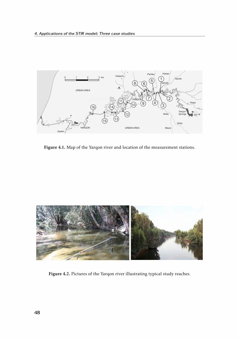
4. Applications of the STIR model: Three case studies
YARQON
Hadarim
Shillo
Shillo
Mazor
Pardes Hadas
Qanah
Qanah
URBAN AREA
URBAN AREAYARQON
Ayalon
YarqonSprings
Raba
1
47
91011
12
568
2
3
13
14
15
16
0 1 2 3 km
Figure 4.1. Map of the Yarqon river and location of the measurement stations.
Figure 4.2. Pictures of the Yarqon river illustrating typical study reaches.
48

4.2 Site description
4.2.2 The Brenton torrent, Italy
The Brenton torrent is an Italian torrential stream located in the area of Treviso
in Northern Italy. The tributary catchment has an area of approximately 60km2;
the elevation from the average sea level varies from 45 to 496m; the length of the
channel is about 13.5km with an average slope of 4.2‰.
The Brenton catchment basin was formed for the most part by the deposition
of sediments transported by the Piave river since the last glaciations. The trans-
ported sediments are primarily coarse debris of grit and limestone. The bed is
made of a thick, high permeable layer of gravel and is characterized by the pres-
ence of iron hydroxide due to the dissolving and hydrolyzing effect that meteoric
waters, containing carbonic acid, exert on the gravel.
The overall length of the study reach is about 5.8km and is characterized by
an average slope equal to 4.2‰. The channel is primarily straight but has a few
90° bends and a few large radius bends. The channel cross-section is regular with
no flood plains and without sensible variations of the flow cross sectional area,
except for a few localized contractions. The channel bed is almost entirely nat-
ural, with only a few quite short reaches in which the banks are reinforced with
concrete or stone. The banks are thickly vegetated. A map of the Brenton tor-
rent showing the position of the measurement stations of the experimental tests
is given in Figure 4.3. Pictures of typical study reaches are given in Figure 4.4.
4.2.3 The Desturo canal, Italy
The Desturo canal is a small 5.6km-long drainage canal which is part of the
drainage basin of the Venice Lagoon in Northern Italy. The canal is located just
outside of a urban settlement and is used for irrigation proposes. The Desturo
canal is affected by pollution due to distributed inputs of fertilizers used in the
agricultural activity. However, the main sources of pollution are due to input of
49

4. Applications of the STIR model: Three case studies
3
4
5
6
7
89
Brenton torrent
21
0 0.5 1 1.5 km
Figure 4.3. Map of the Brenton torrent and position of the measurement stations.
Figure 4.4. Pictures of the Brenton torrent illustrating typical study reaches.
50

4.3 Stream tracer experiments
1
2
3
45
6
0 0.5 1 1.5 km
Des
turo
canal
Figure 4.5. Map of the Desturo canal and position of the measurement stations.
waters from a waste-water treatment plant of the nearby Monselice village and
to inputs of non-treated water during rain periods from urban drainage systems.
The total length of the study reach is equal to 3300m and has almost uniform
characteristics with few channel bends. The channel cross section is trapezoidal
with flood plains and natural banks. The vegetation on the banks is quite thin,
with virtually no masts and bushes. The sediment bed is made of a sandy-silty
material and at the time of the tests the channel bottom was characterized by
the presence of algae, submerged vegetation, and pieces of marsh reeds. A map
showing the planimetry of the canal and the location of the measurement stations
is given in Figure 4.5. Pictures of a study reach are shown in Figure 4.6.
4.3 Stream tracer experiments
Tracer tests were carried out in the Yarqon river in April 2005, in the Breton
torrent in June-July 2007, and in the Desturo canal in October 2007. The experi-
ments consisted in both instantaneous (slug) and continuous (step) injections of
rhodamine WT (RWT) fluorescent dye. For step injections, a peristaltic pump
was used to ensure a constant continuous rate of input throughout the injection
period. In each test RWT concentrations were measured at two downstream sec-
tions with a sampling period of 10s using portable field fluorometers (Turner
51

4. Applications of the STIR model: Three case studies
Figure 4.6. Pictures of the Desturo canal illustrating a typical study reach.
Design SCUFA). In addition to tracer concentrations, the fluorometers measured
water turbidity, which was then used in the detrend procedure of the tracer BTCs
to remove artifact generated by variations of water turbidity. Part of the curves
are excluded from the analysis presented here due to poor quality of the data,
either because the concentration signal was too noisy or because the tail values
of the concentration curves could not be obtained for sufficiently long times to
permit an unambiguous determination of the model parameters. A summary of
the experimental conditions in terms of injected massM0 and length of the injec-
tion period ∆tinj (with ∆tinj = 0 for slug tests) is given in Table 4.1a for the Yarqon
river, Table 4.2a for the Brenton torrent and Table 4.3a for the Desturo canal.
The location of the injection and the measurement sections was chosen so that
the study reaches could be considered as approximately uniform. The length of
the reaches, L, varies from around 660 to 1900m for the Yarqon river (Table 4.1b),
from 620 to 2160m for the Brenton torrent (Table 4.2b), and from 260 to 340m
for the Desturo canal (Table 4.3b). In all cases, the distance from injection al-
lowed the tracer to be well mixed over the cross-section at the measurement sta-
tions.
52
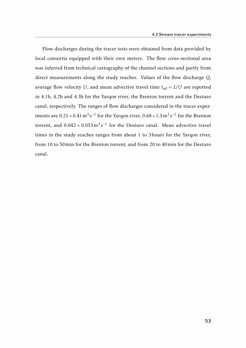
4.3 Stream tracer experiments
Flow discharges during the tracer tests were obtained from data provided by
local consortia equipped with their own meters. The flow cross-sectional area
was inferred from technical cartography of the channel sections and partly from
direct measurements along the study reaches. Values of the flow discharge Q,
average flow velocity U , and mean advective travel time tad = L/U are reported
in 4.1b, 4.2b and 4.3b for the Yarqon river, the Brenton torrent and the Desturo
canal, respectively. The ranges of flow discharges considered in the tracer exper-
iments are 0.21÷0.41m3 s−1 for the Yarqon river, 0.68÷1.5m3 s−1 for the Brenton
torrent, and 0.042 ÷ 0.053m3 s−1 for the Desturo canal. Mean advective travel
times in the study reaches ranges from about 1 to 3hours for the Yarqon river,
from 10 to 50min for the Brenton torrent, and from 20 to 40min for the Desturo
canal.
53

4. Applications of the STIR model: Three case studies
Test 1 2 3
(a) Experimental procedure
M0 (g) 21 21 63 + 53b
∆tinj (s) 0a 0a 3700+0b
(b) Study reaches
Reach 1–5 5–6 8–9 14–16
L (m) 1084 816 657 1887
Q (m3 s−1) 0.21 0.21 0.43 0.41
A (m2) 1.06 2.18 2.71 2.15
tad (s) 5391 8345 4141 9895
(c) Parameters of model with two exponential RTDs
DL (m2 s−1) 0.24 0.25 0.49 2.80
α1 (×10−4 s−1) 7.4 9.4 7.3 7.3
α2 (×10−4 s−1) 0.25 0.78 0 0.54
T1 (s) 163 109 436 340
T2 (s) 2382 1720 — 3781
RMSEc (×10−2) 1.36 4.36 10.29 5.85
(d) Parameters of power-law RTD model
DL (m2 s−1) 0.42 0.20 1.88 3.80
α (×10−2 s−1) 0.29 0.20 1.02 0.42
κc 2.05 1.74 2.67 1.86
RMSEc (×10−2) 3.26 5.41 8.03 7.10
a ∆tinj = 0 indicates an instantaneous (slug) injection.b In Test 3 a mass of tracer of 63g was injected continuously for a period of 3700s after which
a slug injection of 53g was performed at t = 3700s.c The parameters RMSE and κ are unitless.
Table 4.1. Summary of test and model parameters for the Yarqon river.
54
4.3 Stream tracer experiments
Test 1 2 3
(a) Experimental procedure
M0 (g) 50.3 50.3 30.0
∆tinj (s) 780 780 600
(b) Study reaches
Reach 5–6 6–7 6–8 6–9
L (m) 620 1080 1560 2160
Q (m3 s−1) 1.5 1.5 1.5 0.68
A (m2) 1.45 1.34 1.57 0.96
tad (s) 599 962 1632 3036
(c) Parameters of model with two exponential RTDs
DL (m2 s−1) 1.98 2.01 1.85 1.95
α1 (×10−4 s−1) 2.8 15.5 5.0 4.9
α2 (×10−4 s−1) 0.26 0.11 0.18 0.06
T1 (s) 51 52 66 104
T2 (s) 733 912 1081 1735
RMSEa (×10−2) 4.94 2.53 3.26 2.90
(d) Parameters of power-law RTD model
DL (m2 s−1) 2.58 4.75 3.79 3.50
α (×10−2 s−1) 0.010 0.342 0.072 0.167
κa 1.17 2.63 1.93 2.36
RMSEa (×10−2) 5.07 3.19 4.49 3.86
a The parameters κ and RMSE are unitless.
Table 4.2. Summary of test and model parameters for the Brenton torrent.
55

4. Applications of the STIR model: Three case studies
Test 1 2 3
(a) Experimental procedure
M0 (g) 3.24 3.24 3.24
∆tinj (s) 1500 1320 1260
(b) Study reaches
Reach 1–2 2–3 3–4 5–6
L (m) 262 305 336 278
Q (m3 s−1) 0.045 0.045 0.053 0.042
tad (s) 1114 1440 2329 2040
(c) Parameters of model with two exponential RTDs
A (m2) 0.19 0.21 0.36 0.31
DL (m2 s−1) 0.10 0.14 0.09 0.10
α1 (×10−4 s−1) 13.5 10.1 11.0 11.0
α2 (×10−4 s−1) 2.73 1.50 0.70 4.27
T1 (s) 99 171 140 60
T2 (s) 367 365 397 280
RMSEa (×10−2) 2.02 5.40 1.96 4.29
(d) Parameters of power-law RTD model
DL (m2 s−1) 0.84 1.08 0.37 0.38
α (×10−2 s−1) 0.56 0.72 0.57 0.55
κa 2.22 2.43 2.46 2.40
RMSEa (×10−2) 5.48 5.93 3.73 5.54
a The parameters κ and RMSE are unitless.
Table 4.3. Summary of test and model parameters for the Desturo canal.
56

4.4 Solute transport modeling
4.4 Solute transport modeling
RWT tracer transport along the study reaches was simulated using the STIR
model for general residence time distribution modeling. As shown in Chapter 3,
under the assumption of Fickian transport in the surface water in the main chan-
nel, the STIR model is equivalent to the following advection-dispersion-mass-
transfer equation:
∂CW (x, t)∂t
+U∂CW (x, t)
∂x=DL
∂2CW (x, t)∂x2 −α
(CW (x, t)−
∫ t
0CW (x, t − τ)ϕ(τ)dτ
),
(4.1)
where CW (x, t) is the solute concentration in the surface water [ML−3], U is the
average flow velocity [LT−1], given by the ratio of the flow rate and the average
flow cross-sectional area U = Q/A, DL is the longitudinal dispersion coefficient
[L2 T−1], α is the rate of transfer [T−1], and ϕ(t) is the probability density function
(PDF) of the residence times in the storage zones [T−1]. The assumption of unifor-
mity along the study reach implies that U , DL, α and the PDF ϕ(t) are constant
in time and space.
In Chapter 3 it was shown that the overall residence time distribution (RTD)
in a stream segment of length L can be expressed in the Laplace domain as:
r̃(t;x) = r̃W (s+α(1− ϕ̃(s));L) , (4.2)
where r̃W is the Laplace transform of the residence time distribution in the main
channel. In the time domain equation (4.2) implies the following series expan-
sion:
r(t;x) =∞∑m=0
∫ t
0rW (τ ;L)
(ατ)m
m!eατ (ϕ(t − τ))∗m dτ , (4.3)
where (ϕ(t))∗m denotes the m-fold convolution of the function ϕ(t) with itself.
Estimating the residence time distribution in the storage zones from a tracer
57
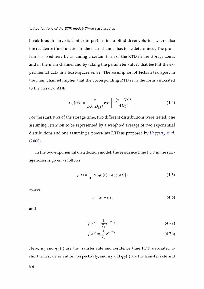
4. Applications of the STIR model: Three case studies
breakthrough curve is similar to performing a blind deconvolution where also
the residence time function in the main channel has to be determined. The prob-
lem is solved here by assuming a certain form of the RTD in the storage zones
and in the main channel and by taking the parameter values that best-fit the ex-
perimental data in a least-square sense. The assumption of Fickian transport in
the main channel implies that the corresponding RTD is in the form associated
to the classical ADE:
rW (t;x) =x
2√πDLt3
exp[−(x −Ut)2
4DLt
]. (4.4)
For the stastistics of the storage time, two different distributions were tested: one
assuming retention to be represented by a weighted average of two exponential
distributions and one assuming a power-law RTD as proposed by Haggerty et al.
(2000).
In the two-exponential distribution model, the residence time PDF in the stor-
age zones is given as follows:
ϕ(t) =1α
[α1ϕ1(t) +α2ϕ2(t)] , (4.5)
where
α = α1 +α2 , (4.6)
and
ϕ1(t) =1T1e−t/T1 , (4.7a)
ϕ2(t) =1T2e−t/T2 . (4.7b)
Here, α1 and ϕ1(t) are the transfer rate and residence time PDF associated to
short timescale retention, respectively, and α2 and ϕ2(t) are the transfer rate and
58
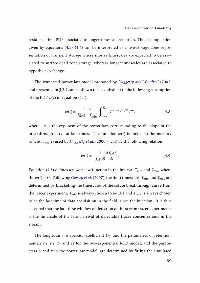
4.4 Solute transport modeling
residence time PDF associated to longer timescale retention. The decomposition
given by equations (4.5)–(4.6) can be interpreted as a two-storage zone repre-
sentation of transient storage where shorter timescales are expected to be asso-
ciated to surface dead zone storage, whereas longer timescales are associated to
hyporheic exchange.
The truncated power-law model proposed by Haggerty and Wondzell (2002)
and presented in § 2.4 can be shown to be equivalent to the following assumption
of the PDF ϕ(t) in equation (4.1):
ϕ(t) =1−κ
T 1−κmax − T 1−κ
min
∫ Tmax
Tmin
T −1−κe−t/T dT , (4.8)
where −κ is the exponent of the power-law, corresponding to the slope of the
breakthrough curve at late times. The function ϕ(t) is linked to the memory
function fM(t) used by Haggerty et al. (2000, § 2.4) by the following relation:
ϕ(t) = − 1fM(0)
dfM(t)dt
. (4.9)
Equation (4.8) defines a power-law function in the interval Tmin and Tmax where
theϕ(t) ∼ tκ. Following Gooseff et al. (2007), the limit timescales Tmin and Tmax are
determined by bracketing the timescales of the solute breakthrough curve from
the tracer experiment; Tmin is always chosen to be 10s and Tmax is always chosen
to be the last time of data acquisition in the field, since the injection. It is thus
accepted that the late-time window of detection of the stream tracer experiments
is the timescale of the latest arrival of detectable tracer concentrations in the
stream.
The longitudinal dispersion coefficient DL, and the parameters of retention,
namely α1, α2, T1 and T2 for the two-exponential RTD model, and the param-
eters α and κ in the power-law model, are determined by fitting the simulated
59

4. Applications of the STIR model: Three case studies
breakthrough curves to the experimental data. Model calibration is performed in
mixed-scale using a linear scale to fit the bulk of the curve and log-scale to fit the
tail. In the optimization procedure the following root mean square is minimized:
RMSE =
1N
∑i∈IU
(Csim,i −Cobs,i
)2(maxi∈I Cobs,i −mini∈I Cobs
)2
+
∑I∈IL
(logCsim,i − logCobs,i
)2(maxi∈I logCobs,i −mini∈I logCobs,i
)2
1/2
(4.10)
where Cobs and Csim are the observed and simulated concentration values, re-
spectively, IU and IL are the sets of the observed values higher and lower than a
given threshold concentration, respectively, I = IU ∪ IL is the total set, and N is
the number of elements in I . The threshold value was set equal to 20% of the
peak concentration. Particular care was taken in calculating min(logCobs,i) by
neglecting the concentration values closer to zero, generally by excluding from
the computation 5% of the total set corresponding to the lowest values. The
optimization was performed using the differential evolution method for global
optimization by Storn and Price (1997, see also Price et al., 2005).
4.5 Results and discussion
Transient storage processes in natural streams generate a delay in the down-
stream transport of a tracer inducing longer tails in the observed BTCs and in-
creasing the skewness of the concentration distributions. Here, the STIR solute
transport model has been used in combination with tracer test data to character-
ize transient storage in three case studies.
The results of the calibration of the STIR model with the two-exponential clo-
sure for the storage time distribution are presented in Table 4.1c, 4.2c and 4.3c
for the Yarqon river, the Brenton torrent and the Desturo canal, respectively. A
graphical comparison between the experimental data and the simulated break-
60
4.5 Results and discussion
through curves is given in Figure 4.7 for the Yarqon river, Figure 4.8 for the Bren-
ton torrent, and in Figure 4.9 for the Desturo canal. The curves are plotted in both
linear and semi-log scale to emphasize their tail behavior, on which the retention
parameters are primarily dependent.
In the study reaches of the Yarqon river the average timescale T1 of fast tran-
sient storage varies from 163 to 436s, with an average value of 262 ± 152s (Ta-
ble 4.1c). The mean residence time T2 associated to long timescale retention
varies from 1720 to 3781s and appears to be higher for increasing average ad-
vective residence times tad. In Reach 8–9 of Test 2, the optimization procedure
converges to α2 ≈ 0, whereas the timescale T1 converges to a value higher the
other reaches (T1 = 436s), indicating that a single exponential distribution is suf-
ficient in this case to adequately represent the BTC. In the study reaches of the
Brenton torrent T1 ranges from 51s to 104s, with an average value of 68 ± 25s,
and it is clearly higher for increasing tad (Table 4.2c). The same increasing trend is
visible for the timescale T2 which varies from 733 to 1735s as the mean advective
travel time tad increases from 600 to 3000s. In the Desturo canal the timescale T1
ranges from 60s to 171s, with average 117± 48s, whereas T2 ranges from 280 to
397s, with average 352± 50s. In this case, an increasing trend of T1 and T2 with
tad is not evident.
The transfer rates are found to be higher in the Desturo canal, with α1 in the
range (1.0÷1.35)×10−3 s−1 and α2 = (0.70÷4.27)×10−4 s−1, compared to the Bren-
ton torrent where α1 = (0.28÷1.55)×10−3 s−1 and α2 = (0.06÷0.26)×10−4 s−1, and
the Yarqon river, where α1 = (0.73÷ 0.94)× 10−3 s−1 and α2 = (0÷ 0.78)× 10−4 s−1.
It can be noticed that the transfer rate associated to the longer timescale reten-
tion component are at least an order of magnitude lower than the transfer rate
associated to the shorter one. This is consistent with the fact that fast transient
storage in surface dead zones is typically characterized by high exchange fluxes,
whereas the transient storage in the hyporheic zones is associated to relatively
61
4. Applications of the STIR model: Three case studies
2000 4000 6000 8000 10000 120000
20
40
60
80
time (s)
2000 4000 6000 8000 10000 1200010
-1
100
101
102
time (s)
1 1.5 2 2.5
x 104
0
5
10
15
20
25
30
time (s)
1 1.5 2 2.5
x 104
10-1
100
101
102
time (s)
2000 4000 6000 8000 10000 120000
5
10
15
20
time (s)
2000 4000 6000 8000 10000 1200010
-1
100
101
102
time (s)
0 1 2 3 4 5
x 104
0
10
20
30
40
time (s)
0 1 2 3 4 5
x 104
10-1
100
101
102
time (s)
Test 1Reach 5-6
Test 1Reach 5-6
Test 1Reach 1-5
Test 1Reach 1-5(a)
(c)
(e)
(g)
(b)
(d)
(f)
(h)
concentr
ation (
�g L
-1)
concentr
ation (
�g L
-1)
concentr
ation (
�g L
-1)
concentr
ation (
�g L
-1)
concentr
ation (
�g L
-1)
concentr
ation (
�g L
-1)
Observations 2-Exp. RTD model Power-law RTD model
Test 2Reach 8-9
Test 2Reach 8-9
Test 3Reach 14-16
Test 3Reach 14-16
concentr
ation (
�g L
-1)
concentr
ation (
�g L
-1)
Figure 4.7. Observed and simulated breakthrough curves for the Yarqon river (left) in
linear scale and (right) semi-log scale.
62

4.5 Results and discussion
0 500 1000 1500 2000 25000
10
20
30
40
50
time (s)
0 500 1000 1500 2000 250010
-1
100
101
102
time (s)
1000 1500 2000 2500 3000 3500 40000
10
20
30
40
50
time (s)
1000 2000 3000 400010
-1
100
101
102
time (s)
1000 2000 3000 4000 50000
10
20
30
40
50
time (s)
1000 2000 3000 4000 500010
-1
100
101
102
time (s)
2000 3000 4000 5000 6000 70000
10
20
30
40
50
60
time (s)
2000 3000 4000 5000 6000 700010
-1
100
101
102
time (s)
Test 1Reach 5-6
Test 1Reach 5-6(a)
(c)
(e)
(g)
(b)
(d)
(f)
(h)
concentr
ation (
�g L
-1)
concentr
ation (
�g L
-1)
concentr
ation (
�g L
-1)
concentr
ation (
�g L
-1)
concentr
ation (
�g L
-1)
concentr
ation (
�g L
-1)
Observations 2-Exp. RTD model Power-law RTD model
Test 2Reach 6-8
Test 2Reach 6-8
Test 3Reach 8-9
Test 3Reach 8-9
concentr
ation (
�g L
-1)
concentr
ation (
�g L
-1)
Test 1Reach 6-7
Test 1Reach 6-7
Figure 4.8. Observed and simulated breakthrough curves for the Brenton torrent (left)
in linear scale and (right) semi-log scale.
63

4. Applications of the STIR model: Three case studies
0 1000 2000 3000 4000 5000 60000
10
20
30
40
50
time (s)
0 2000 4000 600010
-1
100
101
102
time (s)
0 2000 4000 6000 8000 100000
10
20
30
40
time (s)
0 2000 4000 6000 8000 1000010
-1
100
101
102
time (s)
0 1000 2000 3000 4000 5000 6000 70000
10
20
30
40
50
time (s)
0 2000 4000 600010
-1
100
101
102
time (s)
0 2000 4000 6000 80000
10
20
30
40
50
60
time (s)
0 2000 4000 6000 800010
-1
100
101
102
time (s)
Test 1Reach 1-2
Test 1Reach 1-2(a)
(c)
(e)
(g)
(b)
(d)
(f)
(h)
concentr
ation (
�g L
-1)
concentr
ation (
�g L
-1)
concentr
ation (
�g L
-1)
concentr
ation (
�g L
-1)
concentr
ation (
�g L
-1)
concentr
ation (
�g L
-1)
Observations 2-Exp. RTD model Power-law RTD model
Test 2Reach 3-4
Test 2Reach 3-4
Test 3Reach 5-6
Test 3Reach 5-6
concentr
ation (
�g L
-1)
concentr
ation (
�g L
-1)
Test 1Reach 2-3
Test 1Reach 2-3
Figure 4.9. Observed and simulated breakthrough curves for the Desturo canal (left) in
linear scale and (right) semi-log scale.
64
4.5 Results and discussion
small transfer rates and long residence times. The values of α1 and α2 do not
exhibit particular trends as a function of the average advective travel time, tad.
Despite the apparent dependence of the parameters T1 and T2 on the timescale
of observation, it is possible to compare the retention parameters of the Desturo
canal with the parameters of the Brenton torrent since the range of values of tad
for the reaches of the former overlaps with the range of tad for the reaches of the
latter. The higher values of the timescale T2 characterizing the Brenton torrent
can be seen as a consequence of the higher permeability of the bed, which implies
significant hyporheic fluxes in the subsurface. In the Desturo canal, the low per-
meability of the bed implies that the subsurface fluxes are extremely small, and
the observed retention effects are likely to be primarily due to surface dead zones
and, in particular, to the thick submerged vegetation characterizing the channel
bed. Nevertheless, it is not possible to compare unambiguously the properties
of short timescale retention in the streams analyzed. In the Brenton torrent the
longitudinal dispersion coefficients are an order of magnitude greater than those
found in the Desturo canal, which allows a wider range of retention phenomena
to be lumped in the parameter DL. A proper comparison would require the value
of DL to be determined independently of the retention parameters.
An important parameter of the two-exponential RTD model is given by the
ratio of the two timescales of retention T2/T1. When this ratio is close to 1, the
breakthrough curves can be well represented by a single exponential distribution,
and hence the conventional TSM model with a single storage zone is expected to
provide acceptable approximations of the experimental data. This is the case of
the Desturo canal for which the mean ratio is T2/T1 is 3.3 ± 1.1. In a semi-log
graph, the corresponding breakthrough curves tend to follow a linear pattern af-
ter the concentration peak. High ratios are instead found in the Yarqon river and
the Brenton torrent, for which the average ratio T2/T1 is 11.3± 5.3 and 16.3± 7.1,
respectively. When plotted in semi-log scale, the relevant breakthrough curves
65

4. Applications of the STIR model: Three case studies
shows a long tail behavior. In particular, in the case of the Brenton torrent, the de-
creasing part of the curve is characterized by a clear change of slope (Figure 4.8):
the part of the curve between the concentration peak and the bend is associated
to quicker exchange processes and determines primarily the value of T1 and α1;
the subsequent part the curve is associated to long term retention and is related
to the parameters T2 and α2. The rising part of the curve is mainly associated to
advection and dispersion processes in the main channel and the steepness of the
curve depends primarily on the value on the longitudinal dispersion coefficient.
The results of the parameter calibration for the power-law model are pre-
sented in Table 4.1d, 4.2d and 4.3d for the Yarqon river, the Brenton torrent and
the Desturo canal, respectively. In the Yarqon river the exponent κ ranges from
1.64 to 2.67, and there is no dependence of either κ or α on tad. In the the Bren-
ton torrent the exponent κ varies from 1.17 to 2.63, with higher transfer rates
associated to higher κ. In the Desturo canal, the calibration procedure converged
to values of κ close to 2.4, but the model is clearly unable to represent the late
time behavior of the breakthrough curves as it can be seen by visual inspection of
Figure 4.9. The values of the longitudinal dispersion coefficients obtained with
the power-law RTD model are higher (from 4 to 8 times greater in the Desturo
canal) than those obtained with the two-exponential RTD model. In the case of
the Desturo canal, the values of DL determined with the power-law model do not
seem to be adequate to represent the transport dynamics in the main channel,
since the rising part of the simulated breakthrough curves do not well approxi-
mate the experimental data. The result further suggests that DL should be deter-
mined separately, for example with an adequate hydrodynamic modeling of the
flow in the main channel.
A comparison of the RMSE values for the two models presented shows that,
on the average, the model assuming two exponential RTDs to represent transient
storage provides better fits of the observed concentration data than the truncated
66

4.5 Results and discussion
power-law model. This is not only a consequence of the higher flexibility allowed
by a higher number of calibration parameters: in fact, when plotted in a semi-
log scale, many of the experimental breakthrough curves show linear patterns in
the decreasing part following the concentration peak, indicating an exponential
behavior of the tails. This is particularly evident in the case of the Desturo canal
(Figure 4.9). It should be noted, however, that when the results of the two models
are compared in linear scale, the difference appears rather small.
The methods used in this study does not allow to clearly distinguish between
in-channel and subsurface, hyporheic transient storage. Nevertheless, it is likely
that long BTC tails observed in some of the reaches result from hyporheic ex-
change. The modeling closure assuming transient storage to be represented by
two exponential RTDs allows a simple conceptual separation of fast and slow
exchange: the former is expected to be associated to surface dead zones and the
latter to hyporheic zones. This modeling closure has the property that the two
residence time distributions adopted for fast and slow exchange have the same
functional form, thereby permitting a direct comparison of the timescale param-
eter, that is the mean residence time for an exponential PDF. However, the exper-
imental results presented here seem to suggest that the timescales of retention
T1 and T2 of the two-exponential RTD model are dependent on the spatial and
temporal scale of observation, thus making the parameters difficult to compare
between stream reaches of different travel time. The scale dependent behavior
of the mean residence time is implicit in the power-law RTD model, for which
a mean residence time cannot be defined (Haggerty and Wondzell, 2002). Never-
theless, the power-law model as proposed by Haggerty et al. (2000) did not pro-
vide good approximation of the late time behavior of the observed breakthrough
curves in a number cases.
It is also relevant to note that the storage parameters are expected to be de-
pendent on the flow discharge, which determines both the fluxes and the mean
67
4. Applications of the STIR model: Three case studies
residence times in the storage zones. The main limitation of the tracer test ap-
proach is that it is not possible to generalize the results to conditions different
than those directly observed in the experiments. In Chapter 3 it was shown that
transfer rates can be defined as the ratio of the flux at the stream-storage zone
interface and a length scale, typically the water depth or the hydraulic radius,
both increasing with the flow discharge. The average cross-sectional area AS of
the storage zones is also expected to increase with flow discharge, and the re-
sulting mean residence time depends on the ratio between the storage volume
and the flux into the storage zones. Furthermore, the mixing in the surface water
is known to be dependent on the flow velocity, with higher mixing associated
to higher velocities, which in turn affects the shape of the concentration dis-
tributions. Different retention processes can also be activated by different flow
regimes, making it difficult to make reliable predictions about the behavior of
the storage parameters with different flow discharges.
4.6 Conclusions
Tracer breakthrough curves result from a complex multiple convolution of the
RTD in the main channel and the RTDs in the storage zones. Separating in-
channel transport from transient storage using tracer breakthrough curves is an
ill-posed mathematical problem. Here, tracer test data were analyzed with the
STIR model using the classical inverse approach: a certain functional form was
assumed for the RTD in the storage zones and in the main channel, and the rel-
evant parameters were determined by fitting the model predictions to tracer test
data. Two different modeling closures were tested: one assuming the residence
time statistics in the storage zones to be represented by a weighted average of
two exponential distributions, and one assuming a truncated power-law distri-
bution in the form proposed by Haggerty et al. (2000) (§ 2.4). In both cases the
RTD in the main channel was assumed to be in the form associated to the con-
68
4.6 Conclusions
ventional advection-dispersion equation. Results show that the two-exponential
RTD model is able to represent with excellent approximation the observed break-
through curves in all the study reaches of the three the streams analyzed. The
mean residence times T1 and T2 in the storage zones, which are parameters of the
exponential distributions, were found to be dependent on the timescale of ob-
servation. In particular, T1 and T2 show an increasing trend for increasing mean
advective travel times, tad, suggesting that the storage parameters of two different
streams should be compared only for similar values of tad. Further investigations
are certainly needed to understand the relationship between the timescale of ob-
servation and the calculated storage parameters.
The power-law RTD model provided good fit of the observed concentration
data in some of the study reaches, but in many cases it was found inadequate
to represent the tail behavior of the tracer BTCs. The observed dependence of
the longitudinal dispersion coefficient, DL, on the particular RTD assumed in the
storage zones suggests that tracer test data should be integrated with hydrody-
namic modeling of the surface flow in the main channel. This would allow the
parameters DL and the average flow cross-sectional area A to be determined sep-
arately from transient storage. A deconvolution approach could then be used to
infer the contribution of retention processes to solute transport.
69

Chapter 5Effect of microbial biofilms on the transient storage
of solutes1
5.1 Introduction
Microbial life in streams is often dominated by biofilms (matrix-enclosed com-
munities including bacteria, archaea, algae, fungi and protozoa) coating the sed-
iments (Sigee and Sigee, 2005). Understanding the controls of biofilms on so-
lute transport is essential given the contributions of streams to biogeochemical
fluxes (Battin et al., 2008; Mulholland et al., 2008). Biofilms differentiate into
complex physical structures such as filamentous streamers floating in the water
and thereby adapt to the hydrodynamic conditions (Battin et al., 2003). Biofilm
differentiation also results from interactions between mass transport and conver-
sion processes (Wimpenny and Colasanti, 1997), and from shear-induced erosion
and compacting (Battin et al., 2003). Ultimately, this differentiation can create re-
tention domains at the streambed-streamwater interface, which can act as solute
storage zones in support of biological activity as shown in a range of studies. For
1The contents of this chapter have been published in: Bottacin-Busolin, A., G. Singer,
M. Zaramella, T. J. Battin, and A. Marion (2009), Effects of Streambed Morphology and Biofilm
Growth on the Transient Storage of Solutes, Environ. Sci. Technol., 43 (19), 7337-7342.
71
5. Effect of microbial biofilms on the transient storage of solutes
instance, Kim et al. (1990) and Kim et al. (1992) simulated nitrate retention by
periphytic (i.e., phototrophic) biofilms based on hydrologic advection-dispersion
transport, transient storage (Bencala and Walters, 1983) and Michaelis-Menten
uptake kinetics. Mulholland et al. (1994) used an advection-dispersion model to
show how dispersion coefficients and transient storage zones increase with peri-
phytic biomass. DeAngelis et al. (1995) showed the effect of periphytic biofilms on
stream hydraulics using a single storage zone model, which was then extended
to include hyporheic exchange as a separate retention domain to consider the ef-
fect of periphyton on subsurface nitrogen cycling (Dent and Henry, 1999). Gooseff
et al. (2004) attributed rapid nitrate removal to the transient storage zone cre-
ated by periphytic mats rather than to the hyporheic zone. Recently, Orr et al.
(2009) reported hyporheic processes to dominate nutrient retention when peri-
phytic biomass is low, whereas nutrient retention became allocated to the benthic
zone as biomass developed and clogged the sediments.
In this chapter, results are presented from tracer experiments carried out in
streamside flumes with low submergence-streambeds. The experiments were
designed to evaluate how solute transient storage is mutually affected by bed
morphology and related biofilm. Illuminating this link is important to help re-
store headwater streams. The analysis presented here is based on the theoretical
framework of the STIR model (Chapter 3), which allows for general residence
time modeling of processes acting at different temporal and spatial scales. The
particular method used to determine the parameters of the model allowed to sep-
arate effects of biofilms and bed-induced hydrodynamics.
5.2 Experimental methods
Streambeds were constructed in five streamside flumes (length: 40m, width:
0.4m; Lunz am See, Austria). The bottom of each flume was shaped from imper-
meable bedforms with wavelength λ = 1m, horizontal distance between the crest
72

5.2 Experimental methods
100 cm
H
75 cm
Flow gravel layer
PVC sheath
d
PVC sheath
W
Figure 5.1. Longitudinal sketch of a bedform.
and the upstream trough λc = 0.75m, and height H = 2,4,6,8,10cm, respectively
(Figure 5.1). Bedforms were covered with a single layer of indigenous, clean and
graded (median grain diameter: 9.2mm) sediment which served as substratum
for biofilm growth (Figure 5.2). This set-up with limited size of hyporheic storage
zones simulated stream reaches with bedrock and constrained hyporheic zones.
All flumes were continuously fed from the same header tank with raw stream
water (Oberer Seebach) in a once-through mode to assure identical water chem-
istry and microbial inoculum. Periodically measured concentrations of NO3 −N,
NH4 −N and dissolved organic carbon (DOC) averaged 0.57± 0.24mgL−1 (mean
± standard deviation, n = 22 number of samples), 4.4 ± 4.25µgL−1 (n = 24), and
1.49 ± 0.52mgL−1 (n = 39), respectively. Concentrations of PO4 −P were mostly
below the detection limit (< 3µgL−1). Water temperature averaged 9.1 ± 1.3℃.
The flow rate was adjusted to 2.25 ± 0.10Ls−1 by fixing the water level in the
header tank and checked daily throughout the experiment. Uniform flow condi-
tions were obtained by adjusting a tilting weir at the downstream flume end. The
resulting flow can be described as shallow rough-bed flow as it is typical in nat-
ural headwater streams at base flow. Slopes of the flumes were adjusted to yield
identical flume-scale flow velocities but with increasing spatial heterogeneity of
flow velocity, roughness and water depth.
Sterile unglazed ceramic coupons were used (1 × 2cm), as surrogate for nat-
ural substratum in biofilm studies (Battin et al., 2003; Besemer et al., 2007), to
determine the areal content of chlorophyll-a (Besemer et al., 2007). Coupons were
73
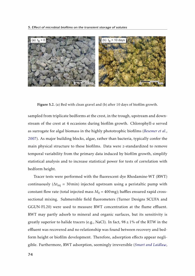
5. Effect of microbial biofilms on the transient storage of solutes
Figure 5.2. (a) Bed with clean gravel and (b) after 10 days of biofilm growth.
sampled from triplicate bedforms at the crest, in the trough, upstream and down-
stream of the crest at 4 occasions during biofilm growth. Chlorophyll-a served
as surrogate for algal biomass in the highly phototrophic biofilms (Besemer et al.,
2007). As major building blocks, algae, rather than bacteria, typically confer the
main physical structure to these biofilms. Data were z-standardized to remove
temporal variability from the primary data induced by biofilm growth, simplify
statistical analysis and to increase statistical power for tests of correlation with
bedform height.
Tracer tests were performed with the fluorescent dye Rhodamine-WT (RWT)
continuously (∆tinj = 30min) injected upstream using a peristaltic pump with
constant flow rate (total injected mass M0 = 400mg); baffles ensured rapid cross-
sectional mixing. Submersible field fluorometers (Turner Designs SCUFA and
GGUN-FL20) were used to measure RWT concentration at the flume effluent.
RWT may partly adsorb to mineral and organic surfaces, but its sensitivity is
greatly superior to halide tracers (e.g., NaCl). In fact, 98± 1% of the RTW in the
effluent was recovered and no relationship was found between recovery and bed-
form height or biofilm development. Therefore, adsorption effects appear negli-
gible. Furthermore, RWT adsorption, seemingly irreversible (Smart and Laidlaw,
74

5.3 Solute transport modeling
1977) and zero-order (Dierberg and DeBusk, 2005), should not affect the shape of
the breakthrough curves.
5.3 Solute transport modeling
The STIR model is used here to describe the transport dynamics of Rhodamine-
WT in the experimental flumes. It is assumed that the transport of RWT in
the surface water is due to advection and Fickian dispersion processes so that
the conventional advection-dispersion equation applies. The exchange dynamics
with the storage zones is assumed to be a temporal Poisson process. As shown
in Chapter 3, under these assumptions the STIR model reduces to the following
equation:
∂CW (x, t)∂t
+U∂CW (x, t)
∂x=DL
∂2CW (x, t)∂x2 −α
(CW (x, t)−
∫ t
0CW (x, t − τ)ϕ(τ)dτ
),
(5.1)
where CW (x, t) is the solute concentration in the surface water [ML−3], U is the
average flow velocity [LT−1], given by the ratio of the flow rate and the average
flow cross-sectional area U = Q/A, DL is the longitudinal dispersion coefficient
[L2 T−1], α is the rate of transfer [T−1], and ϕ(t) is the probability density function
(PDF) of the residence times in the storage zones [T−1]. It is assumed that the
stream reach is uniform, implying that U , DL, α and the PDF ϕ(t) are constant in
time and space.
According to equation (5.1), the retained mass in a given stream reach of
length L can be computed by integrating in space and time the solute fluxed at
the stream-storage zone interface:
MS(t) = A∫ L
0
∫ t
0
αCW (x, t′)−∫ t′
0αCW (x,τ)ϕ(t′ − τ)dτ
dt′dx . (5.2)
75
5. Effect of microbial biofilms on the transient storage of solutes
In the Laplace domain this expression becomes:
M̃S(s) = Aαs
(1− ϕ̃(s))∫ L
0C̃W (x,s)dx . (5.3)
The total retained mass can be used as a storage parameter describing as whole
the effects of retention processes on solute transport in the experimental systems
described here.
5.4 Model calibration
The effect of biofilm on solute retention has been quantified as follows. The
model is fitted to the experimental breakthrough curves relevant to the beds
without biofilm. This allows determining the parameters of the surface trans-
port, DL and A, and the retention parameters due to solute exchange with the
bottom layer of gravel, α(tB = 0) and ϕ(t; tB = 0), where tB is the age of biofilms
[T]. Since comparison between the experimental breakthrough curves at subse-
quent phases of biofilm growth suggests increased retention, the exchange rate
and the storage time function are expressed as follows:
α(tB) = α(tB = 0) + δα(tB) , (5.4a)
ϕ(t; tB) =1
α(tB)[α(0)ϕ(t;0) + δα(tB)δϕ(t; tB)] , (5.4b)
where δα(tB) and δϕ(t; tB) represent the increment with respect to the initial con-
figuration (at tB = 0). These additional terms are determined by fixing the param-
eters of the superficial transport, DL and A, and the previously found retention
parameters α(0) and ϕ(t;0). The resulting exchange rate and retention function
reflect the various effects of biofilms on solute transport. These may include the
storage in biofilm pores, micro-eddies around biofilm streamers, changes in the
near-bed flow field and in the related interfacial hydrodynamic exchange. In this
sense the overall statistics of the residence times in the storage zones should not
76

5.4 Model calibration
be considered as the result of the sum of the residence times in distinct physical
domains.
Determining the parameters of the surface transport and the basic retention
for the bed without biofilm the storage time function was assumed to be repre-
sentable as a normalized sum of two exponential PDFs:
ϕ(t) =1α
2∑i=1
αiTie−t/Ti , (5.5)
where
α =2∑i=1
αi . (5.6)
This assumption corresponds to the following conceptualization of the problem.
Transport processes acting on time scales of the longitudinal advection due to the
mean flow velocity are represented by the advection and dispersion terms and
are considered as part of the superficial transport. Processes acting on longer
time scales are considered retention processes and are split into fast and long
term retention. The use of two exponential PDFs provides good fit of the experi-
mental breakthrough curves, both in linear and log-scale. Conversely, if only on
exponential PDF is used, as in the TSM, it is not possible to obtain acceptable
representation of the tails of the breakthrough curves (Figure 5.3). On the other
hand, if more than two exponential PDFs are used to represent the storage time
function, and a lower bound for the corresponding mean residence time is not
imposed, a portion of what is identified as superficial transport may become part
of the retention processes. Previous studies used an extended version of the TSM
to identify two distinct storage zones with exponential residence time distribu-
tions (Gooseff et al., 2004; Harvey et al., 2005).
A decomposition similar to equations (5.5) and (5.6) is adopted for δϕ(t; tB),
but now an arbitrary large number of exponential PDFs can be used as basis func-
77

5. Effect of microbial biofilms on the transient storage of solutes
Figure 5.3. Experimental observations (dots) and simulated best-fit breakthrough curves
(lines) for biofilm ages tB = 0 and tB = 32days and bedform height ranging fromH = 2cm
to H = 10cm.
78

5.5 Results and discussion
tions. Since the parameters of the superficial transport and of the basic retention
are constant, the solution converges to a unique function δϕ(t; tB) and exchange
rate δα(tB) within the time range of the experimental observations.
Model calibration is performed in mixed-scale using a linear scale to fit the
bulk of the curve and log-scale for the tail using the same methodology described
in § 4.4.
5.5 Results and discussion
Experimental work combined with the STIR model allowed to investigate the
effect of biofilm-induced transient storage as a function of both bed morphology
and biofilm age. The breakthrough curve fitting procedure for the initial configu-
ration of the bed with clean gravel (tB = 0) shows that both exchange rates, α1 and
α2, and the mean residence times in the storage zones, T1 and T2 are characterized
by variations between the flumes up to 20% of their respective mean value; how-
ever, no particular trend was observed (Table 5.1, Figure 5.3). A detailed analysis
of the behavior of these parameters shows that when transfer rates are lower, the
average residence times tend to increase. This behavior is tentatively attributed
to flow irregularities. Only adequately long residence times are represented by
the storage term in the model, while retention processes acting on small time
scales are represented as part of the surface flow field and affect the longitudinal
dispersion coefficient. The long-term retention is expected to be associated with
the bottom layer of gravel, which had similar characteristics for all the flumes.
However, the physically constrained gravel layer prevents deeper exchange into
the bed as expected from bedform-induced pumping (Elliott and Brooks, 1997a,b).
However, the storage effect due to flow detachment and to the formation of a lo-
cal eddy with low velocities downstream of the bedform, constitutes a retention
process acting on the same time scale as the superficial advection and disper-
sion processes. Since the flow is characterized by low submergence, the increase
79

5. Effect of microbial biofilms on the transient storage of solutes
H (cm) 2 4 6 8 10
A (m2) 0.027 0.027 0.027 0.028 0.030
U (ms−1) 0.083 0.083 0.083 0.080 0.075
DL (m2 s−1) 0.019 0.019 0.020 0.028 0.030
α1 (×10−5 s−1) 37.4 33.3 37.3 35.8 34.0
T1 (s) 112 121 100 107 118
α2 (×10−5 s−1) 4.19 3.63 4.61 4.55 3.80
T2 (s) 667 650 603 615 660
Table 5.1. Estimated parameters of the STIR model for beds without biofilm (tB = 0).
in bedform height affects the whole surface flow field by increasing its hetero-
geneity (i.e., the velocity variance), which can be represented by an enhanced
dispersion coefficient. The coefficient DL is almost 60% higher with bedforms of
H = 10cm than of H = 2cm (Table 5.1), and there is a clear increasing trend for
the itermediate flumes. The flow cross-sectional area, A, as well as the average
velocity, U = Q/A, where Q = 2.25Ls−1, are almost constant for all the flumes,
with a slight increasing trend with bedform height. This increase is limited to
10% of the mean value, which is equal to A = 0.028m2 and corresponds to an
average depth dW = 7cm.
Once the parameters for the superficial flow field and the basic retention for
the beds without biofilms are determined, the additional retention parameters δα
and δϕ(t) are estimated for the biofilm ages tB = 8, 18, 26, 32days while holding
the formers fixed. The simulated concentration curves (Figure 5.3) were obtained
by decomposing the additional retention function, δϕ(t), into 3 exponential PDFs
according to equation (5.5) and (5.6). No further improvement of the data fitting
80
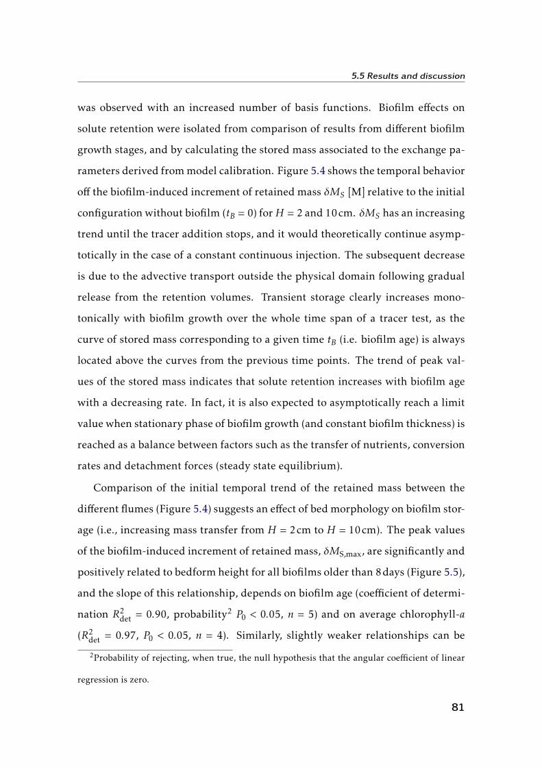
5.5 Results and discussion
was observed with an increased number of basis functions. Biofilm effects on
solute retention were isolated from comparison of results from different biofilm
growth stages, and by calculating the stored mass associated to the exchange pa-
rameters derived from model calibration. Figure 5.4 shows the temporal behavior
off the biofilm-induced increment of retained mass δMS [M] relative to the initial
configuration without biofilm (tB = 0) forH = 2 and 10cm. δMS has an increasing
trend until the tracer addition stops, and it would theoretically continue asymp-
totically in the case of a constant continuous injection. The subsequent decrease
is due to the advective transport outside the physical domain following gradual
release from the retention volumes. Transient storage clearly increases mono-
tonically with biofilm growth over the whole time span of a tracer test, as the
curve of stored mass corresponding to a given time tB (i.e. biofilm age) is always
located above the curves from the previous time points. The trend of peak val-
ues of the stored mass indicates that solute retention increases with biofilm age
with a decreasing rate. In fact, it is also expected to asymptotically reach a limit
value when stationary phase of biofilm growth (and constant biofilm thickness) is
reached as a balance between factors such as the transfer of nutrients, conversion
rates and detachment forces (steady state equilibrium).
Comparison of the initial temporal trend of the retained mass between the
different flumes (Figure 5.4) suggests an effect of bed morphology on biofilm stor-
age (i.e., increasing mass transfer from H = 2cm to H = 10cm). The peak values
of the biofilm-induced increment of retained mass, δMS,max, are significantly and
positively related to bedform height for all biofilms older than 8days (Figure 5.5),
and the slope of this relationship, depends on biofilm age (coefficient of determi-
nation R2det = 0.90, probability2 P0 < 0.05, n = 5) and on average chlorophyll-a
(R2det = 0.97, P0 < 0.05, n = 4). Similarly, slightly weaker relationships can be
2Probability of rejecting, when true, the null hypothesis that the angular coefficient of linear
regression is zero.
81

5. Effect of microbial biofilms on the transient storage of solutes
Figure 5.4. Plots of the increment of retained mass, δMS(t; tB,H) =MS(t; tB,H)−MS(t; tB =
0,H), versus time, t, for different biofilm ages, tB.
82
5.5 Results and discussion
found for MS,max, the peak values of the total retained mass which include the
basic retention for tB = 0 (Figure 5.5). This clearly shows an effect of bedform
height on the ability of biofilms to create additional retention zones, and further
suggests that this effect becomes stronger with biofilm age and biomass. This
could be due to enhanced biofilm growth in flumes with higher bedforms which
would lead to increasingly diverging biomass among the flumes over time and
could explain the trends of δMS,max andMS,max. Indeed, when the observed stan-
dardized values of chlorophyll-a, zChla, are plotted against bedform height (Fig-
ure 5.6), an increasing trend is suggested (R2det = 0.71, P0 < 0.07), indicating that
bed topography may influence the dynamics of biofilm growth leading to a higher
overall biomass in environments with higher heterogeneity. An explanation for
this behavior lies in the increased velocity variance associated with a higher vari-
ability of bed elevation and generating more turbulent flow field, which in turn
ameliorate nutrient transfer. On the other hand, if detachment is limiting biofilm
differentiation, the observed behavior may be due to the downstream shift of the
flow reattachment point for higher bedforms implying an extended zone of low
shear stress. This effect may exceed the increase of shear stress downstream of the
reattachment point up to the crest and induce an overall reduction of the biofilm
detachment rate.
Biofilm biomass (clorophyll-a) explained a large fraction of the variance of
biofilm-induced transient storage δMS,max (Figure 5.7), even though a secondary
effect of bedform height on δMS,max is still visible. A multiple linear regression
model δMS,max as the dependent variable and chlorophyll-a and bedform height
as independents identified significant influences of both predictors (P0 < 0.001
for chlorophyll-a, P0 < 0.05 for bedform height, F-value F2,12 = 52.2, overall P0 <
0.001, adjusted R2det = 0.88). Thus, higher bedforms allow biofilms with the same
chlorophyll-a content to increase their retention capacity.
Residuals from a linear model explaining the biofilm-induced increment of
83
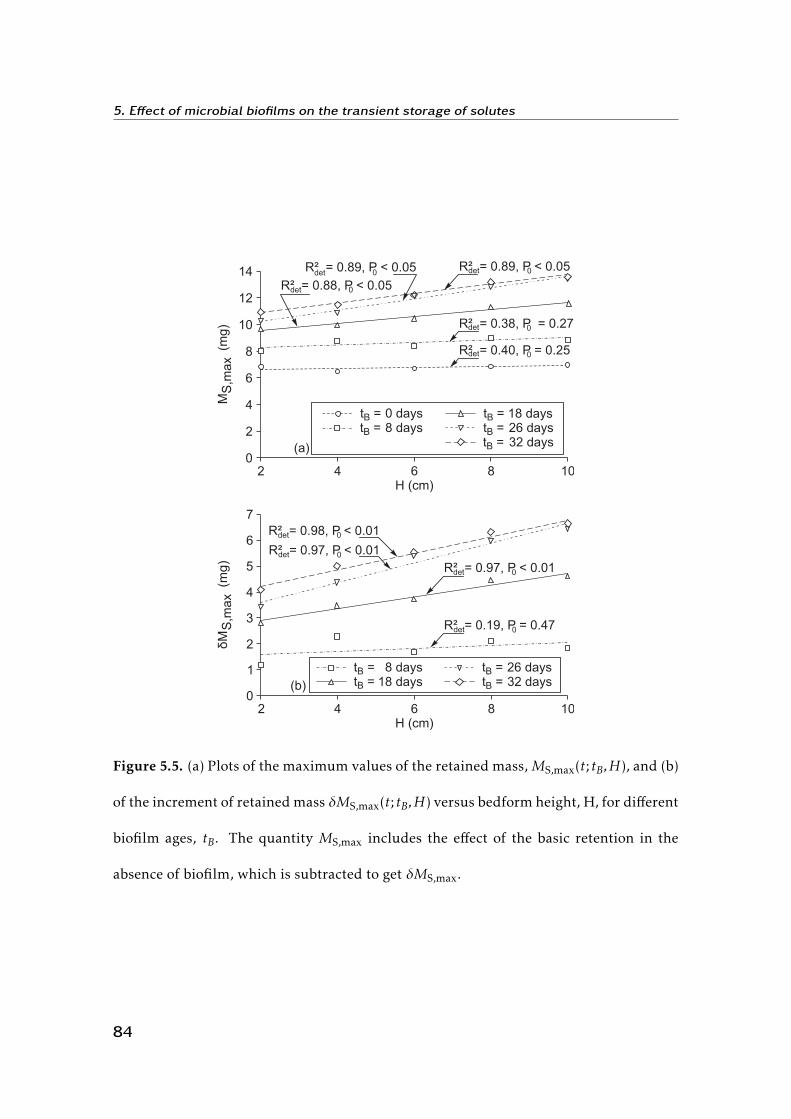
5. Effect of microbial biofilms on the transient storage of solutes
0
2
4
6
8
10
12
14
2 4 6 8 10H (cm)
0
1
2
3
4
5
6
7
R² = 0.88, P < 0.05
R² = 0.89, P < 0.05
R² = 0.38, P = 0.27
R² = 0.40, P = 0.25
R² = 0.89, P < 0.05
2 4 6 8 10H (cm)
R² = 0.19, P = 0.47
R² = 0.97, P < 0.01
R² = 0.98, P < 0.01
R² = 0.97, P < 0.01
δM
(m
g)
S,m
ax
M
(m
g)
S,m
ax
0 days8 days
18 days26 days32 days
t =B
t =B
t =B
t =B
t =B
8 days18 days
26 days32 days
t =B
t =B
t =B
t =B
(a)
(b)
det 0
det 0
0det
det 0
det 0
det 0
det 0
0det
det 0
Figure 5.5. (a) Plots of the maximum values of the retained mass,MS,max(t; tB,H), and (b)
of the increment of retained mass δMS,max(t; tB,H) versus bedform height, H, for different
biofilm ages, tB. The quantity MS,max includes the effect of the basic retention in the
absence of biofilm, which is subtracted to get δMS,max.
84
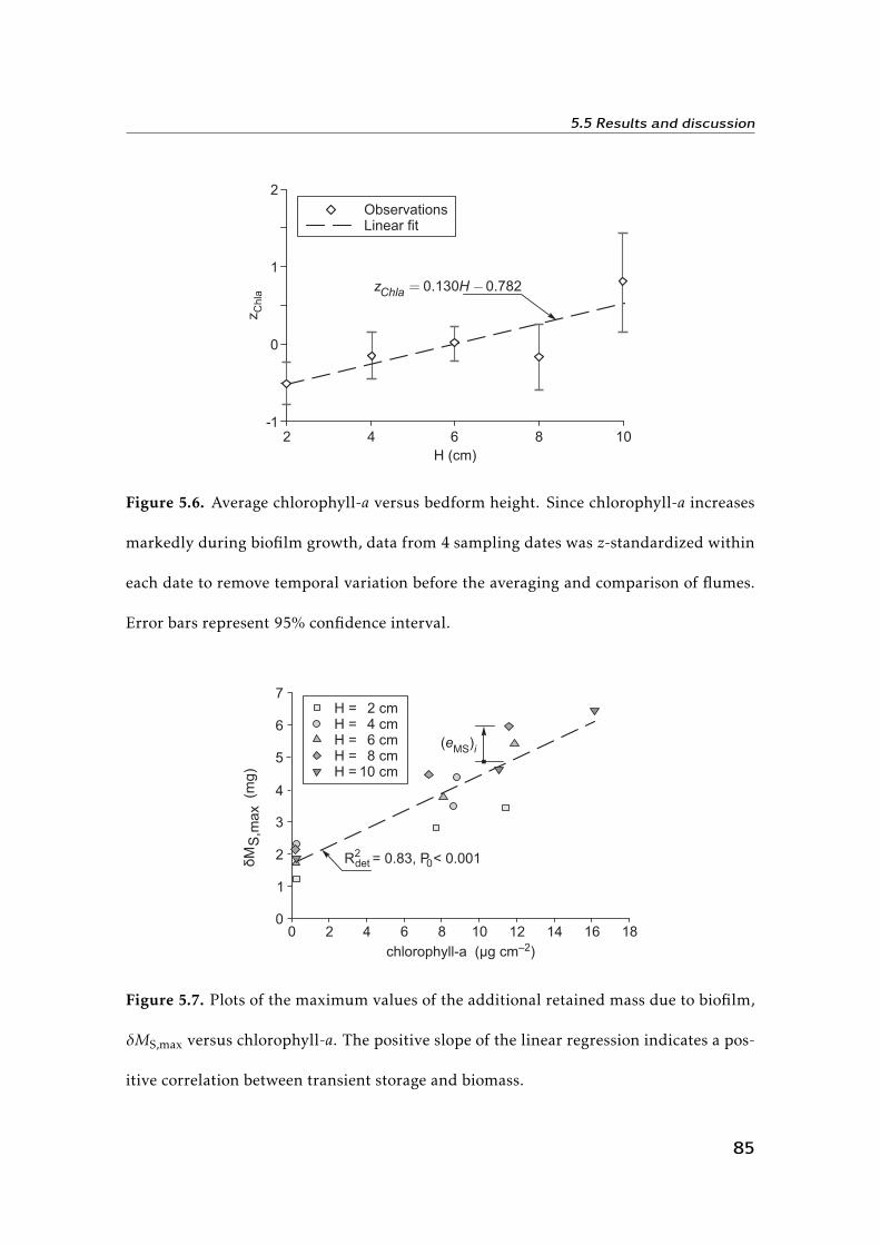
5.5 Results and discussion
-1
0
1
2
2 4 6 8 10
H (cm)
0.130 0.782Chla
z H� �
ObservationsLinear fit
zC
hla
Figure 5.6. Average chlorophyll-a versus bedform height. Since chlorophyll-a increases
markedly during biofilm growth, data from 4 sampling dates was z-standardized within
each date to remove temporal variation before the averaging and comparison of flumes.
Error bars represent 95% confidence interval.
chlorophyll-a ( g cm )μ –2
0 2 4 6 8 10 12 14 16 18
2 cm4 cm6 cm8 cm
10 cm
H =H =H =H =H =
( )eMS i
R = 0.83, P < 0.0012
0
1
2
3
4
5
6
7
δM
(m
g)
S,m
ax
det 0
Figure 5.7. Plots of the maximum values of the additional retained mass due to biofilm,
δMS,max versus chlorophyll-a. The positive slope of the linear regression indicates a pos-
itive correlation between transient storage and biomass.
85
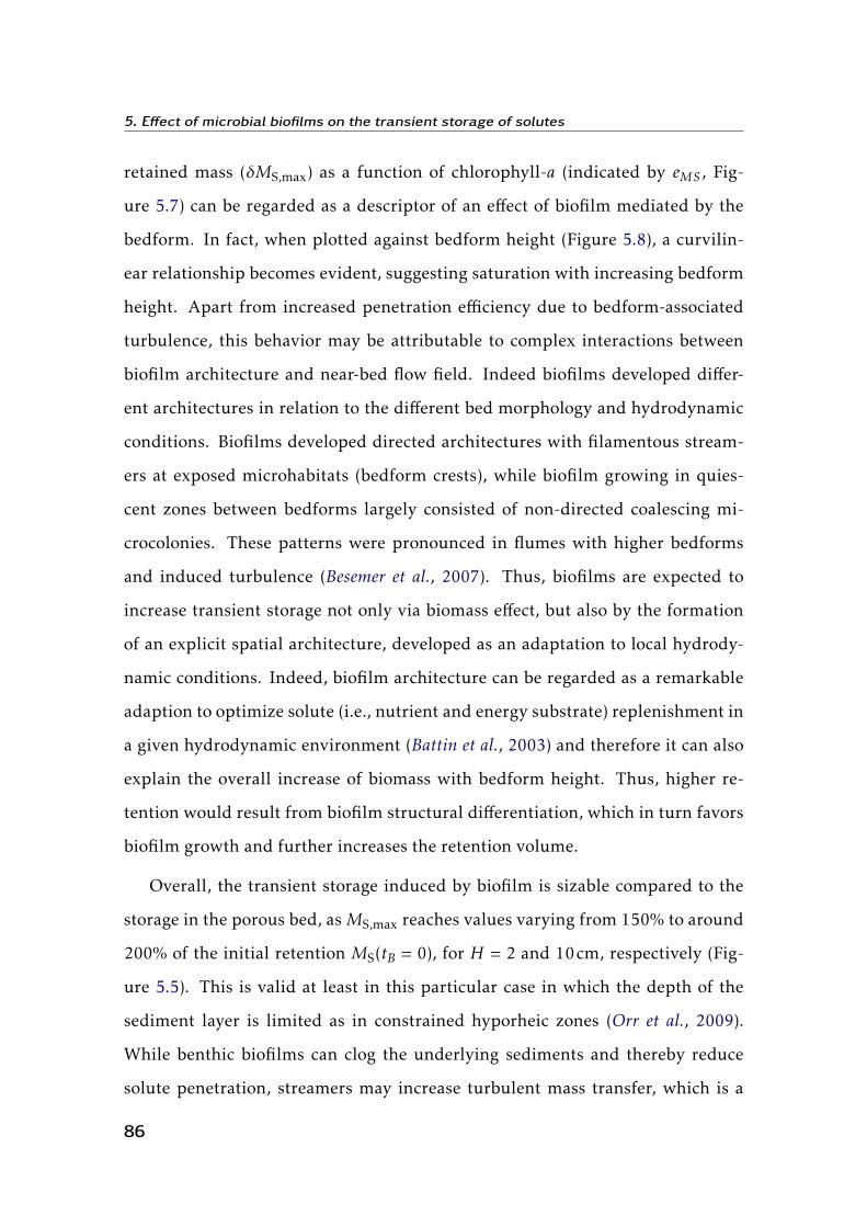
5. Effect of microbial biofilms on the transient storage of solutes
retained mass (δMS,max) as a function of chlorophyll-a (indicated by eMS , Fig-
ure 5.7) can be regarded as a descriptor of an effect of biofilm mediated by the
bedform. In fact, when plotted against bedform height (Figure 5.8), a curvilin-
ear relationship becomes evident, suggesting saturation with increasing bedform
height. Apart from increased penetration efficiency due to bedform-associated
turbulence, this behavior may be attributable to complex interactions between
biofilm architecture and near-bed flow field. Indeed biofilms developed differ-
ent architectures in relation to the different bed morphology and hydrodynamic
conditions. Biofilms developed directed architectures with filamentous stream-
ers at exposed microhabitats (bedform crests), while biofilm growing in quies-
cent zones between bedforms largely consisted of non-directed coalescing mi-
crocolonies. These patterns were pronounced in flumes with higher bedforms
and induced turbulence (Besemer et al., 2007). Thus, biofilms are expected to
increase transient storage not only via biomass effect, but also by the formation
of an explicit spatial architecture, developed as an adaptation to local hydrody-
namic conditions. Indeed, biofilm architecture can be regarded as a remarkable
adaption to optimize solute (i.e., nutrient and energy substrate) replenishment in
a given hydrodynamic environment (Battin et al., 2003) and therefore it can also
explain the overall increase of biomass with bedform height. Thus, higher re-
tention would result from biofilm structural differentiation, which in turn favors
biofilm growth and further increases the retention volume.
Overall, the transient storage induced by biofilm is sizable compared to the
storage in the porous bed, asMS,max reaches values varying from 150% to around
200% of the initial retention MS(tB = 0), for H = 2 and 10cm, respectively (Fig-
ure 5.5). This is valid at least in this particular case in which the depth of the
sediment layer is limited as in constrained hyporheic zones (Orr et al., 2009).
While benthic biofilms can clog the underlying sediments and thereby reduce
solute penetration, streamers may increase turbulent mass transfer, which is a
86
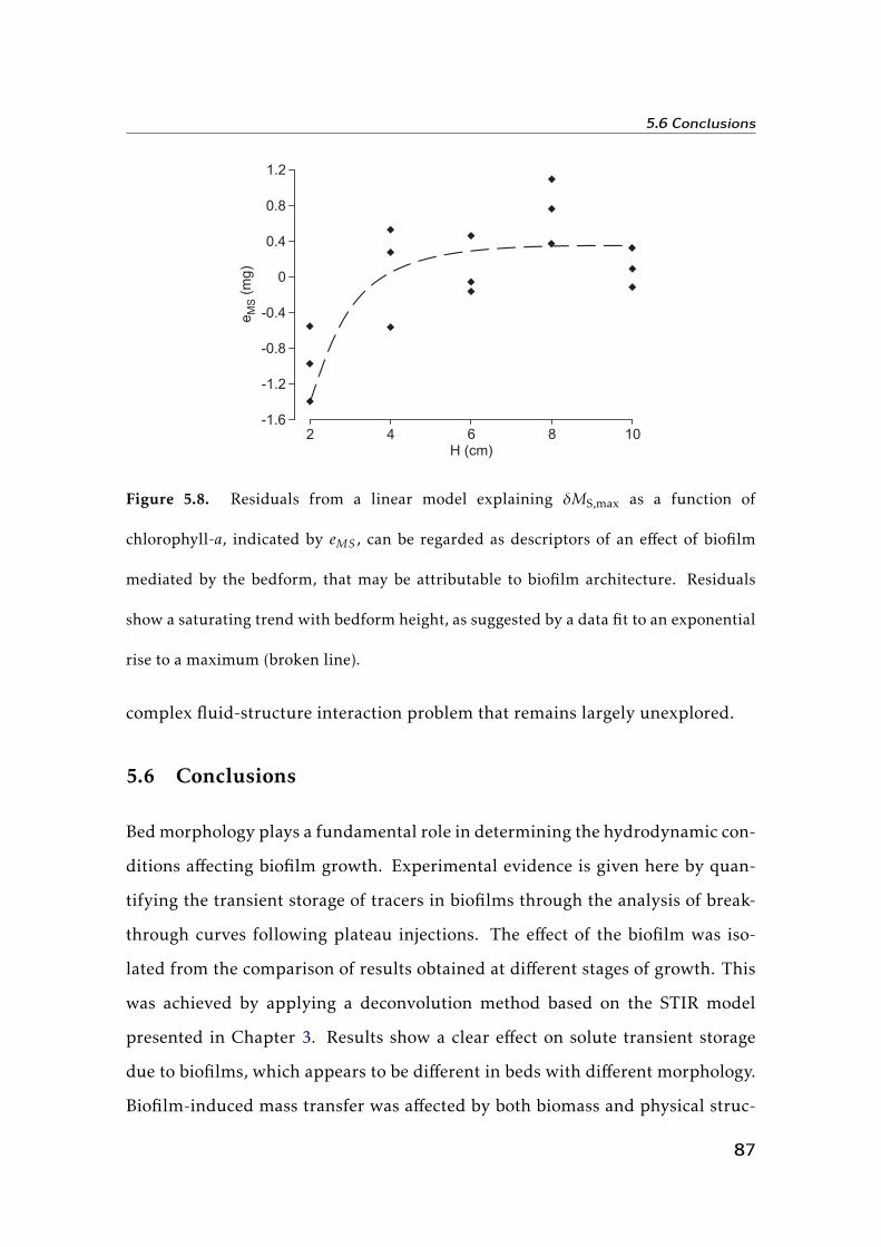
5.6 Conclusions
Figure 5.8. Residuals from a linear model explaining δMS,max as a function of
chlorophyll-a, indicated by eMS , can be regarded as descriptors of an effect of biofilm
mediated by the bedform, that may be attributable to biofilm architecture. Residuals
show a saturating trend with bedform height, as suggested by a data fit to an exponential
rise to a maximum (broken line).
complex fluid-structure interaction problem that remains largely unexplored.
5.6 Conclusions
Bed morphology plays a fundamental role in determining the hydrodynamic con-
ditions affecting biofilm growth. Experimental evidence is given here by quan-
tifying the transient storage of tracers in biofilms through the analysis of break-
through curves following plateau injections. The effect of the biofilm was iso-
lated from the comparison of results obtained at different stages of growth. This
was achieved by applying a deconvolution method based on the STIR model
presented in Chapter 3. Results show a clear effect on solute transient storage
due to biofilms, which appears to be different in beds with different morphology.
Biofilm-induced mass transfer was affected by both biomass and physical struc-
87

5. Effect of microbial biofilms on the transient storage of solutes
ture. Flumes with higher bedforms were found to be characterized by higher
biofilm biomass, which is associated to a larger retention volume. Increasing
bedform height induces biofilms to locally develop hydrodynamically adapted
architectures (e.g., streamers) that can increase the mass transfer into the cavities
of the porous structure of biofilms. The results show the potential of interdis-
ciplinary work combining large-scale experimental set-ups and modeling to un-
ravel basic mechanisms underlying environmental processes related to microbial
biofilms and solute transport dynamics. Technical developments in the area of
flow measurements at the spatial scale of biofilms also open a possible frontier for
future studies. The description of the flow field at such scales will possibly allow
to explain the physical transport processes that are lumped into the calibration
coefficients of an integral transport model such as STIR.
88

Chapter 6Bed form-induced hyporheic exchange in
homogeneous sediment beds1
6.1 Introduction
In the previous chapters a general residence time distribution solute transport
model was presented and applied to a few case studies. In these applications,
particular forms were assumed for the residence time distributions in the stor-
age zones and the relevant parameters were determined by fitting the simulated
breakthrough curves to experimental concentration data from tracer tests. If
enough information is available about the properties of the system under consid-
eration, general residence time transport models can also be used as predictive
tools, at least in principle. Specific modeling closures can indeed be incorporated
to represent retention processes defined on smaller spatial scales than those ex-
amined in tracer tests. This is for example the idea behind the Advective Storage
Path (ASP) model presented by Wörman et al. (2002).
1The contents of this chapter are subject of a paper under review: Bottacin-Busolin, A., and
A. Marion (??), On the combined role of advective pumping and mechanical dispersion in bed
form-induced hyporheic exchange, submitted to Water Resour. Res.
89
6. Bed form-induced hyporheic exchange in homogeneous sediment beds
On very short temporal scales the exchange with the bed is dictated by tur-
bulent diffusion across a thin surficial layer of the bed, usually referred to as the
Brinkman layer. The interfacial diffusion of momentum was originally investi-
gated by Brinkman (1949) and the resulting interaction between the seepage flow
and the free surface turbulent flow above it has subsequently been investigated
by a number of authors (Nagaoka and Ohgaki, 1990; Shimizu et al., 1990; Zhou and
Mendoza, 1993). On longer timescales and larger spatial scales, hyporheic flows
are induced primarily by the interaction of the stream flow with topographical
irregularities of the enclosing boundaries, or by planimetric variations of the flow
direction. Topography-driven hyporheic exchange has been particularly studied
over the years because of its importance in determining the long term response
of a fluvial system to both natural and anthropic inputs of nutrients and con-
taminants. Many works have investigated the effects of topographical features
such as slope irregularities (Harvey and Bencala, 1993), meanders and channel
bends (Boano et al., 2006a; Marion and Zaramella, 2006; Cardenas, 2003; Cardenas
et al., 2004) and alternating bars (Tonina and Buffington, 2007). Bed form-induced
hyporheic exchange in particular has been extensively investigated because bed
forms, such as ripples and dunes, are frequently found in rivers and their effect
can usually be detected within the typical timescales of tracer tests.
Elliott and Brooks (1997a) proposed a conceptual model which came to be
known as the Advective Pumping Model (APM). In the APM surface and subsur-
face flow are decoupled and the effect of the former on the latter is represented
via a sinusoidal pressure variation imposed on a flat surface representing the top
boundary of the bed. Later studies examined how bed form-induced hyporheic
exchange is affected by bed form geometry (Marion et al., 2002; Cardenas and
Wilson, 2007), arbitrary surface topography (Wörman et al., 2006, 2007), hetero-
geneities of the porous medium (Salehin et al., 2004; Marion et al., 2008b; Sawyer
and Cardenas, 2009), physicochemical properties of the transported substances
90

6.2 Solute transport model in the porous medium
(Packman and Brooks, 2001; Packman et al., 2000b,a), unsteady flows (Boano et al.,
2006b), and groundwater discharge (Cardenas and Wilson, 2006; Boano et al.,
2008).
In the present chapter, a few important aspects of bed form-induced hyporheic
exchange are examined adopting some of the simplifying assumptions made by
Elliott and Brooks (1997a). With this approach the effect of the stream gradient
and the propagation of bed forms on the long term behavior of the RTDs is an-
alyzed considering the combined role of advection and pore-scale dispersion in
the porous medium. Simulations show that, at late times, the statistical distri-
butions of the residence time in the bed can show both exponential and power
law behavior, with different exponents associated to advective pumping and pore
scale dispersion. The results provide important clues about the choice of suitable
forms of the RTDs to be used in calibration models such as STIR to identify the
signature of hyporheic retention on solute breakthrough curves.
6.2 Solute transport model in the porous medium
The analysis of the transport of a passive solute in a stream bed is here limited to
two spatial dimensions. A Cartesian frame of reference is adopted where x is the
longitudinal coordinate, oriented along the flow direction, and y is the vertical
coordinate, positive upwards. Following Elliott and Brooks (1997a), the physical
quantity driving the hyporheic flow in the porous medium is represented by a
sinusoidal head distribution imposed on the surface of a semi-infinite flat bed.
The wavelength of the head distribution coincides with the bed form length, in-
dicated by λ, and the amplitude, H , can be linked to the bed form height and
the characteristics of the surface flow. The porous medium is considered to be
isotropic and homogeneous, with uniform hydraulic conductivity, K , and poros-
ity, θ.
91

6. Bed form-induced hyporheic exchange in homogeneous sediment beds
6.2.1 Velocity field
The interaction between streamwater flow and bed forms induces sinusoidal pres-
sure variations over the bed surface. The pressure is lowest over the crest and
separation region downstream of it and rises rapidly to its highest value in the
vicinity of the reattachment region near the base of the upslope. These head vari-
ations induce flowpaths going into the bed where the pressure is higher, and out
of the bed where it is lower. The wavelength of the head fluctuations is equal to
the bed form wavelength, λ, and the amplitude depends on the bed form geom-
etry and flow properties. In case of a stationary bed, the pumping effect induced
by the sinusoidal pressure variation on the bed surface is the main hyporheic ex-
change process driven by bed forms responsible of the penetration penetration of
solutes into the bed.
According to Darcy’s law, the average pore water (seepage) velocity is given
by
u = (u,v) = −K∇h, (6.1)
where u and v are the horizontal and vertical components of the Darcy velocity,
respectively, and h(x,y) is the hydraulic head in the porous medium. The flow of
an incompressible fluid in a homogeneous isotropic bed where Darcy’s law holds
is governed by the Laplace equation
∇2h =∂2h
∂x2 +∂2h
∂y2 = 0 . (6.2)
Equation (6.2) is solved for a semi-infinite porous medium with the following
boundary conditions. On the bed surface, the sinusoidal head variation induced
by bed forms is superimposed to the linear decrease due to the energy gradient
of the overlying stream flow, whereas the sinusoidal head variation vanishes at
92
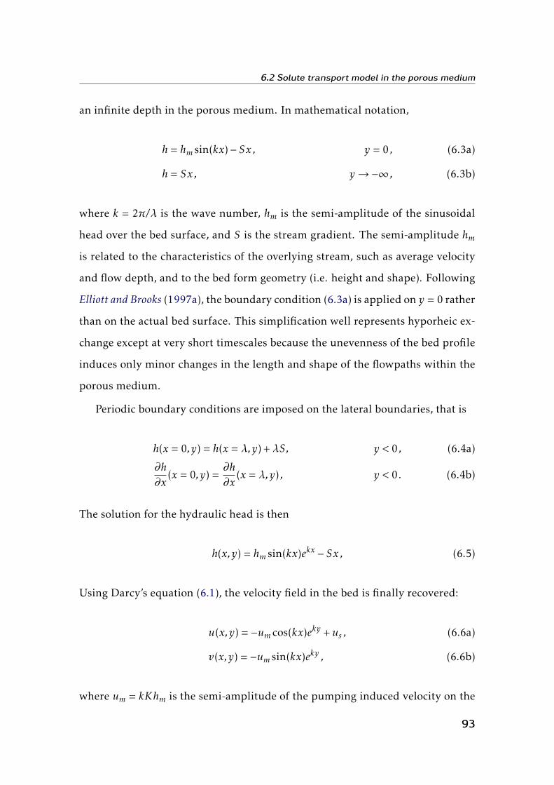
6.2 Solute transport model in the porous medium
an infinite depth in the porous medium. In mathematical notation,
h = hm sin(kx)− Sx , y = 0 , (6.3a)
h = Sx , y→−∞ , (6.3b)
where k = 2π/λ is the wave number, hm is the semi-amplitude of the sinusoidal
head over the bed surface, and S is the stream gradient. The semi-amplitude hm
is related to the characteristics of the overlying stream, such as average velocity
and flow depth, and to the bed form geometry (i.e. height and shape). Following
Elliott and Brooks (1997a), the boundary condition (6.3a) is applied on y = 0 rather
than on the actual bed surface. This simplification well represents hyporheic ex-
change except at very short timescales because the unevenness of the bed profile
induces only minor changes in the length and shape of the flowpaths within the
porous medium.
Periodic boundary conditions are imposed on the lateral boundaries, that is
h(x = 0, y) = h(x = λ,y) +λS, y < 0 , (6.4a)
∂h∂x
(x = 0, y) =∂h∂x
(x = λ,y) , y < 0 . (6.4b)
The solution for the hydraulic head is then
h(x,y) = hm sin(kx)ekx − Sx , (6.5)
Using Darcy’s equation (6.1), the velocity field in the bed is finally recovered:
u(x,y) = −um cos(kx)eky +us , (6.6a)
v(x,y) = −um sin(kx)eky , (6.6b)
where um = kKhm is the semi-amplitude of the pumping induced velocity on the
93
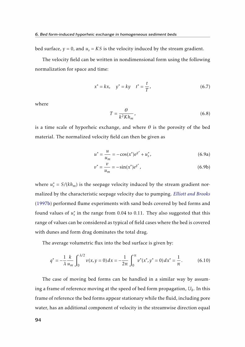
6. Bed form-induced hyporheic exchange in homogeneous sediment beds
bed surface, y = 0, and us = KS is the velocity induced by the stream gradient.
The velocity field can be written in nondimensional form using the following
normalization for space and time:
x∗ = kx, y∗ = ky t∗ =tT, (6.7)
where
T =θ
k2Khm, (6.8)
is a time scale of hyporheic exchange, and where θ is the porosity of the bed
material. The normalized velocity field can then be given as
u∗ =uum
= −cos(x∗)ey∗+u∗s , (6.9a)
v∗ =vum
= −sin(x∗)ey∗, (6.9b)
where u∗s = S/(khm) is the seepage velocity induced by the stream gradient nor-
malized by the characteristic seepage velocity due to pumping. Elliott and Brooks
(1997b) performed flume experiments with sand beds covered by bed forms and
found values of u∗s in the range from 0.04 to 0.11. They also suggested that this
range of values can be considered as typical of field cases where the bed is covered
with dunes and form drag dominates the total drag.
The average volumetric flux into the bed surface is given by:
q∗ = −1λkum
∫ λ/2
0v(x,y = 0)dx = − 1
2π
∫ π
0v∗(x∗, y∗ = 0)dx∗ =
1π. (6.10)
The case of moving bed forms can be handled in a similar way by assum-
ing a frame of reference moving at the speed of bed form propagation, Ub. In this
frame of reference the bed forms appear stationary while the fluid, including pore
water, has an additional component of velocity in the streamwise direction equal
94

6.2 Solute transport model in the porous medium
to −Ub. Far from the bed surface, deep in the porous medium where the pumping
effect is negligible, the pore water appears moving with velocity us/θ−Ub. When
us/θ−Ub = 0, i.e. if the bed form celerity matches the gradient induced underflow,
the velocity field is symmetrical. Typical flowpaths for us/θ −Ub = 0 are shown
in Figure 6.1. When us/θ −Ub , 0, the symmetry disappears and the solutions
can be classified in four cases illustrated in Figure 6.2: (a) −um < us −θUb < 0, (b)
0 < us −θUb < um, (c) us −θUb < −um and (d) us −θUb > um. However, it is impor-
tant to notice that the interface flux, as well as the vertical component of velocity,
are independent of us/θ−Ub, and transport quantities such as penetration depth
and residence times are dependent on the magnitude of us/θ −Ub but are inde-
pendent of its sign. The analysis can therefore be simplified by considering only
the absolute value of the relative underflow velocity, defined in dimensionless
form as
U ∗uf =∣∣∣∣∣us −θUbum
∣∣∣∣∣ =∣∣∣u∗s −U ∗b∣∣∣ . (6.11)
As shown in Figure 6.1, for U ∗uf = 0 two distinct symmetrical advective cells are
visible with flowpaths penetrating indefinitely in the porous medium. ForU ∗uf < 0
(Figure 6.2a-b) the flowpaths outline two nonsymmetrical cells: a smaller one
where the direction of the horizontal velocity component is the same as the un-
derflow, and a larger one where it is mainly opposite. The flowpath separating
the two advective cells converges in a stagnation point at a finite depth. Situation
where U ∗uf < 1 are typical of still or slow moving bed forms.
For rapidly moving bed forms U ∗uf can be higher than 1. In this case (illus-
trated in Figure 6.2c-d) there is only one advective cell, the streamwise compo-
nent of the seepage velocity has the same direction of the underflow and there
is no stagnation point. The flowpath penetrating most deeply in the bed, which
outlines the lower boundary of the advective hyporheic zone, reattaches to the
bed surface in a point of tangency.
95
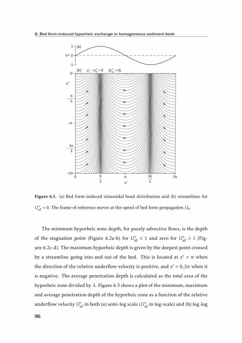
6. Bed form-induced hyporheic exchange in homogeneous sediment beds
π
2
π 2π
π
2�
–π
–2π
0
3π
2�
y�
� � �
� � �0 ( 0)s b uf
u U U(b)
(a)
3π
2
0
x�
1
0
-1
h*
Figure 6.1. (a) Bed form-induced sinusoidal head distribution and (b) streamlines for
U ∗uf = 0. The frame of reference moves at the speed of bed form propagation Ub.
The minimum hyporheic zone depth, for purely advective flows, is the depth
of the stagnation point (Figure 6.2a-b) for U ∗uf < 1 and zero for U ∗uf > 1 (Fig-
ure 6.2c-d). The maximum hyporheic depth is given by the deepest point crossed
by a streamline going into and out of the bed. This is located at x∗ = π when
the direction of the relative underflow velocity is positive, and x∗ = 0,2π when it
is negative. The average penetration depth is calculated as the total area of the
hyporheic zone divided by λ. Figure 6.3 shows a plot of the minimum, maximum
and average penetration depth of the hyporheic zone as a function of the relative
underflow velocity U ∗uf in both (a) semi-log scale (U ∗uf in log-scale) and (b) log-log
96
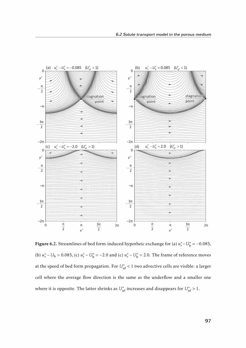
6.2 Solute transport model in the porous medium
(c)� � �
� � �2.0 ( 1)s b uf
u U U
(b)� � �
� � �0.085 ( 1)s b uf
u U U
stagnation
point
stagnation
point
stagnation
point
stagnation
point
stagnation
point
stagnation
point
π
2π 2π3π
20
x�
(d)� � �
� � � �2.0 ( 1)s b uf
u U U
3π
2�
π
2�
–π
–2π
0
y�
(a)� � �
� � � �0.085 ( 1)s b uf
u U U
stagnation
point
stagnation
point
stagnation
point
π
2π 2π3π
20
x�
3π
2�
π
2�
–π
–2π
0
y�
3π
2�
π
2�
–π
–2π
0
y�
3π
2�
π
2�
–π
–2π
0
y�
Figure 6.2. Streamlines of bed form-induced hyporheic exchange for (a) u∗s−U ∗b = −0.085,
(b) u∗s −Ub = 0.085, (c) u∗s −U ∗b = −2.0 and (c) u∗s −U ∗b = 2.0. The frame of reference moves
at the speed of bed form propagation. For U ∗uf < 1 two advective cells are visible: a larger
cell where the average flow direction is the same as the underflow and a smaller one
where it is opposite. The latter shrinks as U ∗uf increases and disappears for U ∗uf > 1.
97

6. Bed form-induced hyporheic exchange in homogeneous sediment beds
scale. The penetration depth decreases linearly with log(U ∗uf) for U ∗uf < 1 and is
inversely proportional to U ∗uf for U ∗uf > 1. An expression that well approximates
the average depth d∗ of the hyporheic zone as a function of U ∗uf is the following
d∗ =
eπ− log(U ∗uf) , U ∗uf < 1 ,
eπ
(U ∗uf)−1 , U ∗uf ≥ 1 ,
(6.12)
where e is the natural base of logarithms. Expression (6.12) was found by inspec-
tion.
6.2.2 Advection-dispersion model
The transport equation for a non-reactive solute in a porous stream bed can be
written as (Zheng and Bennett, 1995)
θ∂C∂t
+∂∂xi
[uiC −θDij
∂C∂xj
]= 0 , (6.13)
where C is the solute concentration, ui are the components of the seepage (Darcy)
velocities, Dij are the components of the hydrodynamic dispersion tensor given
by
θDij = αT |u|δij + (αL −αT )uiuj|u|
. (6.14)
In this study the description of the flow field is limited to two dimensions, hence
i, j = 1,2. In equation (6.14) |u| is the magnitude of the seepage velocity, δij is
Krnocker’s delta, and αL and αT are the longitudinal and transverse dispersivi-
ties, respectively. In most applications, the longitudinal dispersivity can be as-
sumed to be approximately equal to the mean particle size.
Introducing the normalized quantities
C∗ =CC0, u∗i =
uium
, (6.15)
98
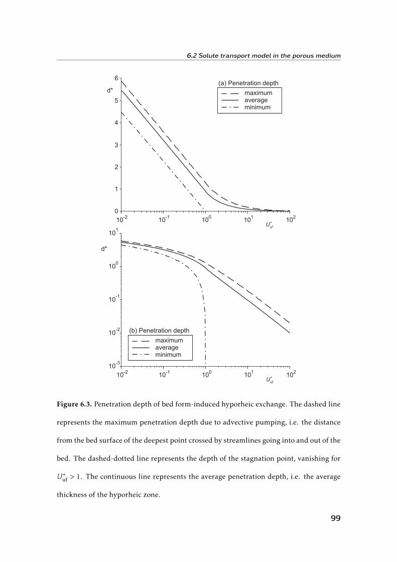
6.2 Solute transport model in the porous medium
(a) Penetration depth
10-2
10-1
100
101
102
ufU
�
0
1
2
3
4
5
6
d* maximumaverageminimum
(b) Penetration depth
maximumaverageminimum
10-3
10-2
10-1
100
101
d*
10-2
10-1
100
101
102
ufU
�
Figure 6.3. Penetration depth of bed form-induced hyporheic exchange. The dashed line
represents the maximum penetration depth due to advective pumping, i.e. the distance
from the bed surface of the deepest point crossed by streamlines going into and out of the
bed. The dashed-dotted line represents the depth of the stagnation point, vanishing for
U ∗uf > 1. The continuous line represents the average penetration depth, i.e. the average
thickness of the hyporheic zone.
99

6. Bed form-induced hyporheic exchange in homogeneous sediment beds
where C0 is a reference concentration, and
D∗ij =θDijKhm
=kθDijum
= α∗T |u∗|δij + (α∗L −α
∗T )u∗iu
∗j
|u∗|, (6.16)
where α∗L = kαL and α∗L = kαT are the dimensionless dispersivities, equation (6.16)
can be written dimensionless form:
∂C∗
∂t∗+∂∂x∗i
u∗iC∗ −D∗ij ∂C∗∂x∗j
= 0 . (6.17)
When adopting a frame reference moving at the speed of bed from propagation,
equation (6.17) remains unaltered and xi and ui are respectively the spatial co-
ordinates and the vertical components relative to the moving frame of reference.
However, the velocity components defining the dispersion tensor in (6.16) are
those relative to the fixed frame of reference.
Equation (6.17) is solved using a modified code from the CLAWPACK soft-
ware library (LeVeque, 1997). The equation is discretized using a finite volume
method which is essentially second order accurate for smooth concentration dis-
tributions and which can also handle step gradients in C∗ (even discontinuities
if D∗ij ≡ 0). This is accomplished via a fractional step method solving the ad-
vection portion of the equation with a high resolution shock-capturing method
and the diffusion equation with an implicit finite-volume discretization. The de-
tails of the algorithm are described in a work by Calhoun and LeVeque (2000). In
solving the equation we tested for grid independence and also checked the so-
lutions for independence on the depth of the lower domain boundary where a
no-flux condition was applied, so that the solutions can be regarded as relevant
to a semi-infinite bed.
100
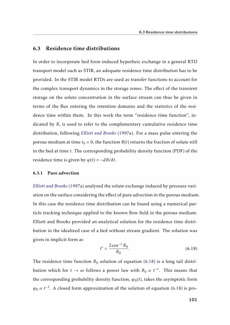
6.3 Residence time distributions
6.3 Residence time distributions
In order to incorporate bed form-induced hyporheic exchange in a general RTD
transport model such as STIR, an adequate residence time distribution has to be
provided. In the STIR model RTDs are used as transfer functions to account for
the complex transport dynamics in the storage zones. The effect of the transient
storage on the solute concentration in the surface stream can thus be given in
terms of the flux entering the retention domains and the statistics of the resi-
dence time within them. In this work the term “residence time function”, in-
dicated by R, is used to refer to the complementary cumulative residence time
distribution, following Elliott and Brooks (1997a). For a mass pulse entering the
porous medium at time t0 = 0, the function R(t) returns the fraction of solute still
in the bed at time t. The corresponding probability density function (PDF) of the
residence time is given by ϕ(t) = −dR/dt.
6.3.1 Pure advection
Elliott and Brooks (1997a) analyzed the solute exchange induced by pressure vari-
ation on the surface considering the effect of pure advection in the porous medium.
In this case the residence time distribution can be found using a numerical par-
ticle tracking technique applied to the known flow field in the porous medium.
Elliott and Brooks provided an analytical solution for the residence time distri-
bution in the idealized case of a bed without stream gradient. The solution was
given in implicit form as
t∗ =2cos−1R0
R0. (6.18)
The residence time function R0 solution of equation (6.18) is a long tail distri-
bution which for t → ∞ follows a power law with R0 ∝ t−1. This means that
the corresponding probability density function, ϕ0(t), takes the asymptotic form
ϕ0 ∝ t−2. A closed form approximation of the solution of equation (6.18) is pro-
101

6. Bed form-induced hyporheic exchange in homogeneous sediment beds
posed here as follows
R0(t∗) = 1− π4
(1− e−βt∗
β− 2
1 + 2/t∗
), (6.19)
where
β =π
2(π − 2). (6.20)
The function (6.19) was found by direct comparison of different functional forms
approximating the numerical solutions of equation (6.18) and represents an alter-
native of the probability density function given by Marion and Zaramella (2005b)
(see § 3.2.4). This form is easier to handle because it has a closed form integral
and has a simpler Laplace transform (which is often useful for semi-analytical
solution of transport models such as STIR or CTRW).
In the case of a gradient induced underflow the RTD no longer follows a
power-law indefinitely, because the flowpaths are confined in a zone of finite
thickness. When U ∗uf < 1, the power-law behavior of the tail is visible only up to a
given timescale. The presence of a stagnation point in the flow field (Figure 6.2a-
b) implies that there is no finite maximum residence time, but at longer times the
R function rapidly decays to zero following an exponential law. In order to give
an analytical form to R(t∗) it must be noted that R(t∗) overlaps with R0(t∗) (equa-
tion (6.19)) at initial times and that it follows an exponential decay as t∗ → ∞.
Inspection of the form of R(t∗) leads to an analytical approximation in which
two timescales are specifically introduced as a function of U ∗uf. The function R is
shown to be approximated extremely well by the following expression
R(t∗;U ∗uf) = R(t∗;U ∗uf, t
∗c(U
∗uf), t
∗d(U ∗uf)
)=
=R0(t∗)exp
[−(t∗/t∗c)
1+U ∗uf)]+R0(t∗c)
1 +R0(t∗c)· 1 + et
∗c/t∗d
et∗/t∗d + et
∗c/t∗d, for U ∗uf < 1 ,
(6.21)
where t∗c and t∗d are two timescales linked to the velocity U ∗uf. They can be deter-
102

6.3 Residence time distributions
mined by fitting (6.21) to the residence time functions calculated by numerical
particle tracking. The values of t∗c and t∗d resulting from the least-square fitting of
R forU ∗uf in the range between 0.01 and 1 are plotted in Figure 6.4. A comparison
between the residence time function numerically derived and the approximating
function (6.21) is shown in Figure 6.5 for a few values of the velocity U ∗uf loga-
rithmically spaced in the range between 0.01 and 0.95. As shown in Figure 6.4, t∗c
and t∗d appear to follow a power-law except in a small range of values of U ∗uf very
close to 1, where the approximation error associated to (6.21) rapidly increases.
An approximation for t∗c and t∗d is given by
t∗c = 2t∗d =4U ∗uf
. (6.22)
When the function (6.21) is used in combination with (6.22), the mean relative
error of log(R) for R values in the range 10−7 < R < 1 is less than 3% for U ∗uf < 0.66
and less than 5% for U ∗uf < 0.75.
To understand the meaning of the timescales t∗c and t∗d , we observe that at
early times, i.e. t � t∗d � t∗c, R(t∗)→ R0(t∗). Another property of equation (6.21)
is that, for t∗ > t∗c > t∗d , R ∼ e−t∗/t
∗d , where the symbol ∼ means “asymptotically
proportional to”. In a semi-log graph the tail of R follows a straight line and the
slope is a function of t∗d . The time t∗c can be considered as the timescale at which
R(t∗) diverges from the idealized behavior given by R0(t∗) and begins to decrease
exponentially with decay rate t∗−1d . Since R0 exhibits a power-law behavior for
about t∗ > 10, with R0 ∼ t−2, t∗c can be seen as the timescale for transition between
the power-law and the exponential decay of R, provided that t∗c � 10 (i.e. U ∗uf�
0.4).
When the relative velocity of the underflow is higher than maximum pumping
velocity U ∗uf > 1), the flowpaths are confined in a single advective cell, and a
stagnation point is no longer present. From a residence time perspective, this
103

6. Bed form-induced hyporheic exchange in homogeneous sediment beds
Figure 6.4. Timescales of the residence time distributions for U ∗uf < 1 in case of pure
advective transport in the porous medium. t∗c represents the timescale at which the resi-
dence time function R departs from the ideal solution for U ∗uf = 0, namely R0, and begins
to decrease exponentially with decay rate t∗−1d (R ∼ e−(t∗−t∗c)/t∗d ).
implies the existence of a finite maximum residence time, t∗max. For U ∗uf� 1, t∗max
is linked to U ∗uf by the following approximation
t∗max = 2π(U ∗−1uf +U ∗−4
uf ) , (6.23)
and the residence time is beta-distributed in the interval [0, t∗max]. However, for
U ∗uf � 1 the advective zone is so thin that the effect of the real shape of the bed
forms, both in terms of height and aspect ratio, becomes significant, and the si-
nusoidal model no longer provides an adequate description of the interfacial ex-
change dynamics. Nevertheless, the sinusoidal head model can still be used to
assess, at least qualitatively, the relative importance of advective pumping and
mechanical dispersion.
104

6.3 Residence time distributions
100
101
102
103
104
t*10
-1
10-4
10-3
10-2
10-1
100
R
10-5
0 200 400 600 800 1000t*
10-4
10-3
10-2
10-1
100
R
10-5
U = 0.95uf*
modelapproximation
U =
0.9
5uf
*
U =
0.0
1uf
*
U=
0uf*
(a)
modelapproximation
(b)
U = 0uf*
U = 0.01uf*
U = 0.95uf*
Figure 6.5. Complementary cumulative distributions of the residence time within the
bed plotted in (a) log-log scale and (b) log-linear scale. The gray dotted lines represent
the distributions obtained by numerical particle tracking and accounts solely for the ad-
vective transport in the porous medium. The continuous black lines represents analytical
approximations given by equation (6.21). The RTDs display a power-law behavior where
R ∼ t−1 up to a certain timescale after which the probability decays exponentially with
time.
105
6. Bed form-induced hyporheic exchange in homogeneous sediment beds
6.3.2 Effect of pore-scale dispersion
The residence time distributions in the porous medium are derived by solving
the advection-dispersion equation (6.17) for a step injection of a constant con-
centration C∗0 = 1 at the downwelling boundary, 0 ≤ x∗ ≤ π,
C∗ = 0 , t < 0 , (6.24a)
C∗ = C∗0 = 1 , t∗ ≥ 0 . (6.24b)
The residence time function is then calculated as
R(t∗) = 1− 12πq∗C∗0
∫ 2π
πv∗(x∗)C∗(x∗, t∗)dx∗ , (6.25)
where 2πq∗ = 2 is the flow rate per unit width into the bed at the downwelling
boundary.
Figure 6.6 presents the simulated residence time functions resulting from the
advection-dispersion model compared to the corresponding functions in case of
pure advective transport in the porous medium. The curves in Figure 6.6 were
obtained for u∗s = 0.1 considering values of U ∗uf in the range 0 ÷ 5 and three dif-
ferent values of the dispersivities, namely (a) α∗L = 0.006, (b) α∗L = 0.06 and (c)
α∗L = 0.6 thus covering a broad range of situations. In the simulations the ration
αT /αL was assumed to be constant and equal to 1/3 as suggested in other studies
(Benekos, 2005; Zheng and Bennett, 1995; Qian et al., 2008). Note that each dis-
tribution must be characterized both in terms of U ∗uf and u∗s because even when
adopting a moving frame of reference the dispersion tensor still depends on the
actual seepage velocity, and not the relative one. This means the case of disper-
sive transport is more complex to analyze because the statistics of the residence
time is characterized by two more degrees of freedom relative to the pure ad-
vective case. In fact the RTD depends on 3 parameters (at least): the relative
106

6.3 Residence time distributions
underflow velocity U ∗uf, the seepage velocity induced by the stream gradient u∗s
and the dispersivity α∗L, the ratio αT /αL being taken as fixed.
Pore-scale dispersion induces longer tails in the residence time distributions
(Figure 6.6) by producing a net downward-directed flux at the interface between
the advection dominated pumping zone and the underlying porous medium.
This flux is associated to permanent mass loss which implies that a fraction of
the solute entering the bed has infinite residence time. When the dispersivities
are high, the purely advective model can significantly underestimate the mass
transfer into the bed at late times. In the dispersion dominated region, where
the RTD diverges from the prediction of the advective model, the R function ex-
hibits a pattern similar to a power-law. If the dispersion tensor was constant, R(t)
would diverge from the pure advective case following a power-law with exponent
−1/2 (R ∼ t−1/2). Since the dispersion tensor is related to the seepage velocity ac-
cording to (6.16), thus varying along the y-direction and assuming a constant
value where the underflow velocity is not affected by pumping, the tail of the
R function shows a more complex behavior resulting in R ∼ t−1/2 only at later
timescales (Figure 6.6). At earlier times, pore-scale dispersion induces a pattern
that can be approximated by a power-law with exponents lower than −1/2. As
shown in Figure 6.7, the seepage velocity u∗s affects the tail of R in the dispersion
dominated region inducing longer residence times as u∗s increases, consistently
with the increase of the components of the dispersion tensor (equation (6.16)).
Nevertheless, for the range of values determined in laboratory experiments by
Elliott and Brooks (1997b), namely u∗s = 0.04 ÷ 0.11, and indicated as typical of
field situations where the form drag dominates the total drag, the variations of R
for a given U ∗uf are rather small.
Depending on the values of the underflow velocity and of the dispersivities,
the effect of dispersion is visible at different timescales. The tails of the R func-
tion can be divided in different time ranges to which different functional forms
107
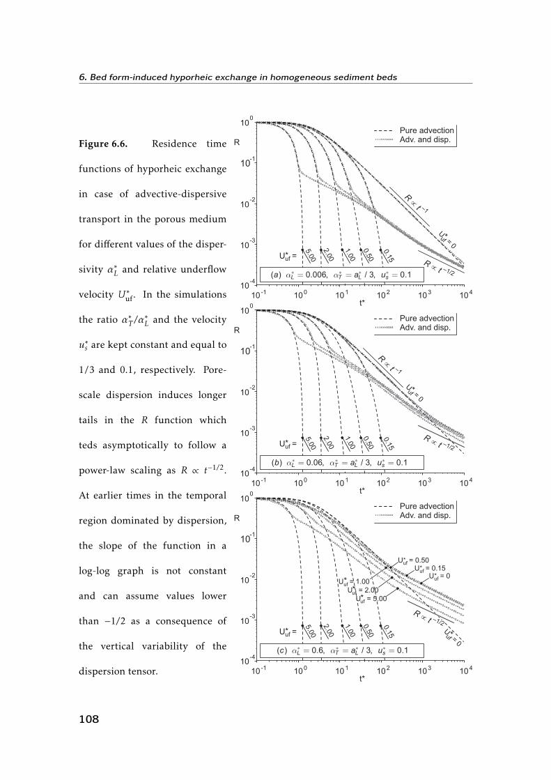
6. Bed form-induced hyporheic exchange in homogeneous sediment beds
Figure 6.6. Residence time
functions of hyporheic exchange
in case of advective-dispersive
transport in the porous medium
for different values of the disper-
sivity α∗L and relative underflow
velocity U ∗uf. In the simulations
the ratio α∗T /α∗L and the velocity
u∗s are kept constant and equal to
1/3 and 0.1, respectively. Pore-
scale dispersion induces longer
tails in the R function which
teds asymptotically to follow a
power-law scaling as R ∝ t−1/2.
At earlier times in the temporal
region dominated by dispersion,
the slope of the function in a
log-log graph is not constant
and can assume values lower
than −1/2 as a consequence of
the vertical variability of the
dispersion tensor.
U = 0.50*uf
U = 0.15*uf
U = 2.00*uf
U = 1.00*uf
U = 0*uf
U = 5.00*uf
R
t�
–1
R
t� –1/2
U=
0
*uf
100
101
102
103
104
t*10
-110
-4
10-3
10-2
10-1
100
R
Pure advectionAdv. and disp.
U =*uf
5.0
0
2.0
0
1.0
0
0.5
0
0.1
5
( ) 0.006, / 3, 0.1L T L sa a u� �� � � �
� � �
R
t�
–1
U=
0
*uf
R
t� –1/2
100
101
102
103
104
t*10
-110
-4
10-3
10-2
10-1
100
R
Pure advectionAdv. and disp.
U =*uf
5.0
0
2.0
0
1.0
0
0.5
0
0.1
5
( ) 0.06, / 3, 0.1L T L sb a u� �� � � �
� � �
U = 0.50*uf
U = 0.15*uf
U = 2.00*uf
U = 1.00*uf
U = 0*uf
U = 5.00*uf
U=
0
*uf
R
t� –1/2
R
t� –1/2
R
t� –1/2
100
101
102
103
104
t*10
-110
-4
10-3
10-2
10-1
100
R
Pure advectionAdv. and disp.
U =*uf
5.0
0
2.0
0
1.0
0
0.5
0
0.1
5
( ) 0.6, / 3, 0.1L T L sc a u� �� � � �
� � �
108
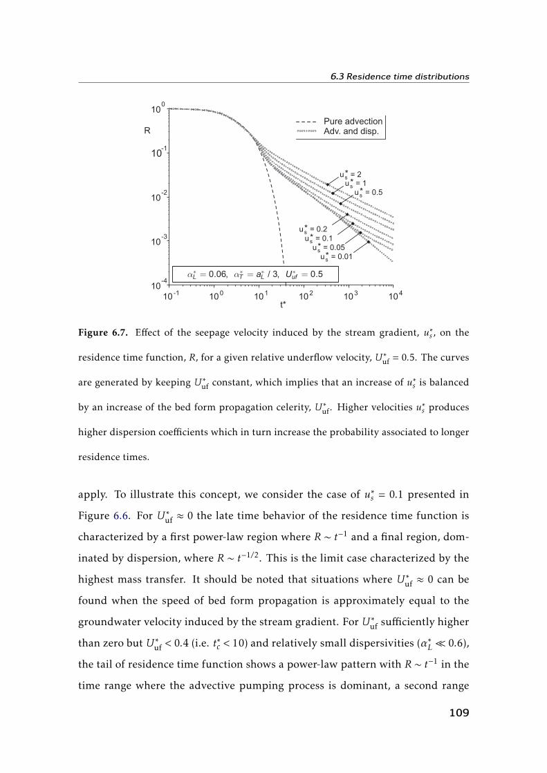
6.3 Residence time distributions
Pure advectionAdv. and disp.
10-4
10-3
10-2
10-1
100
R
100
101
102
103
104
t*10
-1
0.06, / 3, 0.5L T L ufa U� �� � � �
� � �
u = 0.01*s
u = 0.05*s
u = 0.1*s
u = 0.2*s
u = 2*s
u = 1*s
u = 0.5*s
Figure 6.7. Effect of the seepage velocity induced by the stream gradient, u∗s , on the
residence time function, R, for a given relative underflow velocity, U ∗uf = 0.5. The curves
are generated by keeping U ∗uf constant, which implies that an increase of u∗s is balanced
by an increase of the bed form propagation celerity, U ∗uf. Higher velocities u∗s produces
higher dispersion coefficients which in turn increase the probability associated to longer
residence times.
apply. To illustrate this concept, we consider the case of u∗s = 0.1 presented in
Figure 6.6. For U ∗uf ≈ 0 the late time behavior of the residence time function is
characterized by a first power-law region where R ∼ t−1 and a final region, dom-
inated by dispersion, where R ∼ t−1/2. This is the limit case characterized by the
highest mass transfer. It should be noted that situations where U ∗uf ≈ 0 can be
found when the speed of bed form propagation is approximately equal to the
groundwater velocity induced by the stream gradient. For U ∗uf sufficiently higher
than zero but U ∗uf < 0.4 (i.e. t∗c < 10) and relatively small dispersivities (α∗L� 0.6),
the tail of residence time function shows a power-law pattern with R ∼ t−1 in the
time range where the advective pumping process is dominant, a second range
109
6. Bed form-induced hyporheic exchange in homogeneous sediment beds
where the function decays exponentially (R ∼ e−t∗/t∗d ) due to the limiting effect of
the underflow, and then another temporal region, when the exchange process is
dominated by mechanical dispersion, where R tends to be asymptotically propor-
tional to t−1/2 but with slightly lower exponents at earlier times. For 0.4 < U ∗uf < 1,
the tail is characterized by an exponential region followed by a power law region
where R ∼ t−1/2 at late time. When U ∗uf� 1 the effect of advective pumping early
becomes negligible compared to the effect of dispersion which is the only process
responsible for the long term behavior of the residence time function. The result
would not sensibly change if the effect of turnover is accounted for. Indeed, pore-
scale dispersion can well explain the discrepancy observed by Elliott and Brooks
(1997b) between the prediction of their turnover model and their experimental
results: the turnover model greatly underestimated the exchange for moving bed
forms, especially in case of high propagation speeds, and the penetrated mass
was found to be increasing with t1/2.
As the dispersivity of the porous medium increases, the exchange process is
dominated by dispersion at increasingly earlier timescales. When the dispersivity
is high, as shown Figure 6.6c for α∗L = 0.6, dispersion is the dominant process
affecting the whole tail of R. In this situation the effect of the vertical variability
of the dispersion tensor is even more evident: the slope of R in a log-log graph is
lower than −1/2 in a wide temporal range and R ∼ t−1/2 only at late times.
6.4 Discussion
In experimental tracer tests, the late time behavior of breakthrough curves is
recognized to be the signature of long term retention typically associated to hy-
porheic exchange. The results presented here show that distinct functional forms
of the residence time distributions apply in appropriate time ranges. The tempo-
ral extension of these regions depends on the characteristics of the surface flow
and the sediment bed. Although these results were derived for a semi-infinite
110
6.4 Discussion
bed, a qualitative description of how the results would change in case of a per-
meable bed of limited thickness can be given on conceptual basis.
It is known from solutions of the one-dimensional diffusion equation (e.g.
Polyanin, 2002) that, when a constant concentration is imposed at one of the
edges of a bounded domain and a no-flux condition is applied at the other edge,
the ingoing flux decreases exponentially at late times. In the case of bed form-
induced exchange, this implies that, when the penetration is limited by an imper-
meable boundary placed deeper underneath the pumping-dominated advective
zone, the final part of the residence time distribution displays an exponential de-
cay. This behavior characterizes the temporal range in which the limiting effect of
the impermeable boundary significantly affects the vertical concentration profile,
whereas at earlier times the distributions remain unaltered. On the other hand,
if the thickness of the permeable layer is small enough to affect the flowpaths
induced by the bed form-associated pumping effect, and if the relative underflow
velocity is low enough to allow the formation of a stagnation point in the flow
field within the bed, then the maximum residence time is infinite (at least from a
mathematical perspective), but the associated probability must rapidly decrease
to zero at late times, most probably exponentially.
Wörman et al. (2002) suggested that the statistics of the residence time of bed
form-induced hyporheic exchange could be represented by a lognormal distri-
bution. For stationary bed forms and typical groundwater velocities induced by
the stream gradient, a comparison in linear scale shows that, for properly cho-
sen parameters, a lognormal distribution can be a good approximation of equa-
tion (6.21). Nevertheless, when the distributions are compared in a logarithmic
scale, their tail behavior appears substantially different, and even more different
if the effect of dispersion is accounted for. The importance of comparing model
simulations to concentration data in log(concentration) scale at late time has been
increasingly recognized in the recent years. Recent studies have shown that tracer
111
6. Bed form-induced hyporheic exchange in homogeneous sediment beds
breakthrough curves often exhibit a long tail behavior that may be in the form of
power-law patterns. Haggerty and Wondzell (2002) reported data from a tracer
test in a 2nd-order mountain stream in which the tail of the breakthrough curve
followed a power-law scaling as t−1/3 over at least 1.5 orders of magnitude in
time. Gooseff et al. (2003b) performed tracer tests in different reaches of a moun-
tain stream and found that the experimental curves could be well approximated
using a truncated power-law RTD to represent transient storage, with exponents
ranging from −1.6 to −1.3. More recently Gooseff et al. (2007) reported data from
tracer tests performed in streams of different channel complexity. Part of them
could be represented by a conventional model assuming an exponential RTD, but
a few of them displayed power-law patterns with exponents in the range between
−1.9 and −1.7. Although the substrate material of the streambed in these tracer
studies was primarily gravel, cobbles and bedrock, to which the pumping the-
ory does not apply, it can be noticed that exponents of the power-law reported
lie chiefly between −2 and −3/2, the values associated to advective pumping and
dispersion, respectively. Intermediate exponents between −2 and −3/2 have been
shown to arise as a consequence of the vertical variability of the dispersion tensor,
but can also be due to the multi-convolution of the residence time distributions
of many bed forms arranged in sequence. Heterogeneity of the porous medium
may also play a role in defining the apparent exponent of the power-law (Sawyer
and Cardenas, 2009). On the other hand, exponents higher than −3/2, indicating
a slower release of solutes from the storage zones, cannot be explained within the
modeling framework presented here.
The direct application of the multiple region description given in this chap-
ter to real water courses appears at the moment quite difficult given the level of
indetermination of the physical quantities of the system, e.g. sediment perme-
ability, hydraulic conductivity and dispersivity. Tracer tests remain the simplest
way to extract information about hyporheic exchange in field applications. The
112

6.4 Discussion
uncertainty arising from the superposition of surface and subsurface retention
processes requires that the number of parameters involved in transport mod-
els is kept to the minimum necessary to get an acceptable representation of the
observed breakthrough curves. The introduction of two distinct exponential dis-
tributions, as suggested by some authors (Harvey et al., 2005; Briggs et al., 2009),
is the simplest way to move from a single RTD, as for instance in the Transient
Storage Model (Bencala and Walters, 1983), to multiple RTDs. Recent contribu-
tions by Briggs et al. (2009) and the analysis presented in Chapter 4 show that
models with two exponential RTDs are flexible enough to be successfully cal-
ibrated with field tracer data. The results presented in this chapter show that
an exponential distribution can well approximate the statistics of the residence
time in hyporheic zones of limited thickness. When advective pumping or me-
chanical dispersion in the porous medium are dominant processes, the use of two
exponential RTDs may still provide acceptable results in field tracer applications.
This is because the typical timescales of observations are relatively short due to
constraints imposed by instrumental detection limits. However, the power-law
behavior of the RTD associated to advective pumping and pore-scale dispersion
implies that the mean residence time in the hyporheic zones is scale dependent
as observed Chapter 4. Power-law patterns requires accurate measures over a
wide range of timescales to become clearly recognizable. Over smaller tempo-
ral ranges the difference between a power-law and an exponential behavior may
not be detectable without uncertainty. However, when the tails of the observed
breakthrough curves exhibit seemingly power-law patterns with exponents close
to −2 or −3/2, this can be regarded as a fingerprint of bed from-induced advective
pumping and subsurface dispersion affecting a significant portion of the porous
medium. The latter can also be associated to a significant mass loss.
113

6. Bed form-induced hyporheic exchange in homogeneous sediment beds
6.5 Conclusions
Simulations have shown that the residence time distributions of bed form-induced
hyporheic exchange are characterized by a complex tail behavior due to the com-
bination of advective transport and pore-scale dispersion in the porous medium.
At different stage of the exchange process, the RTDs are characterized by differ-
ent functional forms. When the bed form-induced advective pumping is a dom-
inant process and the flowpaths are not limited by an underlying groundwater
flow or by an impermeable boundary, the probability density function of the res-
idence time, ϕ(t), asymptotically tends to a power-law decaying as t−2 (R ∼ t−1).
The combination of the seepage velocity induced by the stream gradient, and the
celerity of the translating bed forms in case of a moving bed, results in a limita-
tion of the advective transport into deeper portions of the porous medium and
causes the PDF to rapidly decay to zero if only advection is accounted for. When
the underflow velocity relative to a frame of reference moving at the speed of bed
form propagation is lower than the maximum pumping-induced velocity, ϕ(t)
decays exponentially, ϕ ∼ e−t/td (R ∼ e−t/td ), and the slope in a semi-log graph
depends on a properly defined timescale td . When the relative velocity of the
underflow is higher than the maximum pumping-induced velocity, the residence
time varies in a bounded time interval and is beta-distributed within it. Pore-
scale dispersion counteracts the limiting effect of the relative underflow velocity
producing longer tails in the RTDs. In the time ranges dominated by dispersion
the PDF ϕ(t) follows a power-law tending to ϕ ∼ t−3/2 at late times (R ∼ t−1/2),
and slightly lower exponents can be found at earlier times as a consequence of
the vertical variability of the dispersion tensor.
The results presented highlight that both exponential and power-law patterns
in the late time behavior of solute breakthrough curves can be associated to hy-
porheic exchange. When the first prevail, the thickness of the hyporheic zone
114
6.5 Conclusions
is limited, whereas, when the second prevails, there is deeper exchange with
the bed that may be due to advective pumping or mechanical dispersion. The
identification of power-law patterns in the breakthrough curves of tracer tests re-
quires measurement over a wide range of timescales, often not available because
of instrumental detection limits. This limitation can make calibration models as-
suming an exponential RTD to represent hyporheic retention sufficient to well
reproduce the observed breakthrough curves, even when the mass transfer is not
limited to a surficial layer of the bed. However, power-law with exponents in the
range from −2 to −3/2, when visible, should be regarded as particular signature
of hyporheic exchange affecting a significant portion of the streambed.
115


Chapter 7Bed form-induced hyporheic exchange in stratified
beds1
7.1 Introduction
In the previous chapter, bed form-induced hyporheic exchange was analyzed
assuming that the porous medium is homogeneous. This assumption is often
adopted in hyporheic studies, although stream beds in nature are typically het-
erogeneous. For a related problem, wind pumping through snowpacks, Colbeck
(1989) showed that subsurface layering substantially alters patterns and rates of
pore fluid flow. Salehin et al. (2004) demonstrated that layered sedimentary het-
erogeneity increases the average interfacial flux but tends to limit vertical pen-
etration because it favor horizontal transport through high-permeability layers.
However, that work used an idealized random correlated permeability field be-
cause relatively little is known about in situ structure in permeable sediment
beds. Cardenas et al. (2004, 2003) used structure-imitating interpolation (kriging)
to obtain a 3D reconstruction of modern channel bend deposits based on constant
1The contents of this chapter have been published in: Marion, A., A. I. Packman, M. Zaramella,
and A. Bottacin-Busolin (2008), Hyporheic flows in stratified beds, Water Resour. Res., 44,
W09433.
117

7. Bed form-induced hyporheic exchange in stratified beds
head injection tests and ground-penetrating radar surveys; they used 3D numeri-
cal modeling to investigate the influence of heterogeneity on the hyporheic fluxes,
showing that residence times can decrease or increase compared to the homoge-
neous case depending on the relative positions of the heterogeneities and bed
forms. More recently, the influence of aquifer heterogeneity on solute exchange
with the hyporheic zone was investigated experimentally by in-situ tracer tests
and measurements by Ryan and Boufadel (2006). In their study higher concentra-
tions were found to be in the upper bed sediments when the hydraulics conduc-
tivity was higher than in the lower bed sediments and vice versa. Recently, Sawyer
and Cardenas (2009) presented numerical simulations on heterogeneous cross-
bedded sediments, showing that heterogeneities can alter the residence time dis-
tributions in river beds.
A particular type of heterogeneous structure is given by the presence of hor-
izontal sediment layers of different permeability. Horizontal stratifications char-
acterized by a coarse surface layer of sediment and an underlying layer of lower
permeability are often found in rivers due to the preferential removal of fines
from the bed surface by entrainment or winnowing. This process is described as
armoring, and the resulting layer of coarse sediments is called armored layer. The
thickness of the armor layer is normally limited to twice the size of the largest
material in the sediment mixture and it is expected to be particularly important
for transport processes acting at short time scales and small spatial scales, at
which diffusion of momentum plays an important role. When the vertical struc-
ture of a porous bed is characterized by an upper coarse layer of sediment thicker
than a typical armor layer, the effect of the heterogeneous structure on hyporheic
exchange can be visible at longer time scales, at which the interfacial turbulent
diffusion is no longer the main transport mechanism in the porous medium. In
this chapter, a model is presented to simulate hyporheic exchange for the case of
bed form-induced hyporheic exchange in presence of two well defined layers of
118
7.2 Hyporheic flow modeling for layered beds
different permeability. The predictions of the model are compared to experimen-
tal data.
7.2 Hyporheic flow modeling for layered beds
7.2.1 Velocity field in the bed
The advective pore water flow induced within a layered sediment bed is mod-
eled here starting from the assumption that Darcy’s law applies for the pore wa-
ter flow within the sediments. Following Elliott and Brooks (1997a) analysis of
pore water flows under dune-shaped bed forms, the upper boundary condition
is taken as a sinusoidal variation in dynamic pressure with wavelength λ coin-
ciding with the bed form wavelength. The bed is idealized as being composed of
an upper layer of thickness d1 and hydraulic conductivity K1 sitting on top of a
lower layer of thickness d2 and conductivity K2. The bed is considered imperme-
able at the bottom of the lower layer and periodic in the downstream direction.
The pressure head at the bed surface can be written as
h(x,y = 0) = hm sin(kx) , (7.1)
where hm is the half amplitude of the pressure at the surface, k = 2π/λ is the
wave number and x and y are the horizontal and vertical Cartesian coordinates,
respectively (y positive upward).
In the subsurface, the hydraulic head follows Laplace’s equation in two di-
mensions ∇2h = 0, valid for homogeneous porous media. The solution for the
induced subsurface head distribution can be found by solving the Laplace equa-
tion in both layers, while matching the solution at the interface. Symmetry re-
quires that the hydraulic head remains sinusoidal over any horizontal plane with
the same wavelength of the surface forcing. Thus the pressure at the interface
119
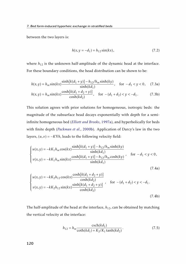
7. Bed form-induced hyporheic exchange in stratified beds
between the two layers is:
h(x,y = −d1) = h12 sin(kx) , (7.2)
where h12 is the unknown half-amplitude of the dynamic head at the interface.
For these boundary conditions, the head distribution can be shown to be:
h(x,y) = hm sin(kx)sinh[k(d1 + y)]− h12/hm sinh(ky)
sinh(kd1), for − d1 < y < 0 , (7.3a)
h(x,y) = hm sin(kx)cosh[k(d1 + d2 + y)]
cosh(kd2), for − (d1 + d2) < y < −d1 . (7.3b)
This solution agrees with prior solutions for homogeneous, isotropic beds: the
magnitude of the subsurface head decays exponentially with depth for a semi-
infinite homogeneous bed (Elliott and Brooks, 1997a), and hyperbolically for beds
with finite depth (Packman et al., 2000b). Application of Darcy’s law in the two
layers, (u,v) = −K∇h, leads to the following velocity field:
u(x,y) = −kK1hm cos(kx)
sinh[k(d1 + y)]− h12/hm sinh(ky)sinh(kd1)
v(x,y) = −kK1hm sin(kx)cosh[k(d1 + y)]− h12/hm cosh(ky)
sinh(kd1)
, for − d1 < y < 0 ,
(7.4a)u(x,y) = −kK2h12 cos(kx)
cosh[k(d1 + d2 + y)]cosh(kd2)
v(x,y) = −kK2h12 sin(kx)sinh[k(d1 + d2 + y)]
cosh(kd2)
, for − (d1 + d2) < y < −d1 .
(7.4b)
The half-amplitude of the head at the interface, h12, can be obtained by matching
the vertical velocity at the interface:
h12 = hmcsch(kd1)
coth(kd1) +K2/K1 tanh(kd2). (7.5)
120

7.2 Hyporheic flow modeling for layered beds
Defining the non-dimensional ratios h∗12 = h12/hm and K∗ = K1/K2, a dimension-
less solution for the subsurface velocity field can be obtained by dividing the
velocity components in equation (7.4) by the velocity scale of pumping defined
as um = kK1hm:
u∗ =
ukK1hm
= −cos(x∗)sinh(d∗1 + y∗)− h∗12 sinh(y∗)
sinh(y∗)
v∗ =v
kK1hm= −sin(x∗)
cosh(d∗1 + y∗)− h∗12 cosh(y∗)sinh(d∗1)
, for − d∗1 < y∗ < 0 , (7.6a)
u∗ =
ukK1hm
= −h12
K∗cos(x∗)
cosh(d∗1 + d∗2 + y∗)cosh(d∗2)
v∗ =v
kK1hm= −sin(x∗)
sinh(d∗1 + d∗2 + y∗)cosh(kd2)
, for − (d∗1 + d∗2) < y∗ < −d∗1 .
(7.6b)
where x∗ = kx, y∗ = ky, d∗1 = kd1 and d∗2 = kd2. The effect of the stream gradient
S and, in case of a moving bed, of velocity of the translating bed forms Ub, can
easily be accounted for by adopting a frame of reference moving at the speed
of bed form propagation and adding to the horizontal streamwise component u∗
in equation (7.6) the velocity u∗s −U ∗b, where u∗s = S/(khm) and U ∗b = θUb/um as
explained in Chapter 6.
The average influx across the stream-subsurface interface is given by the inte-
gral of the vertical velocity,
q =1λ
∫ λ/2
0|v(x,y = 0)|dx = −1
λ
∫ λ/2
0v(x,y = 0)dx . (7.7)
The velocity is integrated between 0 and λ/2 because it is only over this part of
the bed surface that the flux occurs into the bed. The dimensionless average flux
is:
q∗ =q
kK1hm=
1π
[cosh(d∗1)− h∗12
sinh(d∗1)
]. (7.8)
Figure 7.1 shows the streamlines and resulting front positions for a sample
121

7. Bed form-induced hyporheic exchange in stratified beds
3
2��
12
�0
x*
–1
–0.5
0
y*
streamlines front positions
� �12
Figure 7.1. Streamlines and front positions within a homogeneous layered bed. Results
are plotted for a sample case where the ratio between the two hydraulic conductivities is
K∗ = 10 and the dimensionless thickness of the two layers are d∗1 = 0.5 and d∗2 = 0.5. The
longitudinal dimensionless distance scales with the bed form wavelength, x∗ = kx. Front
positions are drawn for non-dimensional timescales t∗ = 0.5, 1, 2, 4 and 16.
case where the ratio between the two hydraulic conductivities is K∗ = 10 and
the dimensionless thickness of the two layers are d∗1 = 0.5 and d∗2 = 0.5. Front
positions are drawn for non-dimensional timescales t∗ = 0.5, 1, 2, 4 and 16. Time
is normalized using the conductivity K1 and porosity θ1 of the upper layer, t∗ =
tk2K1hm/θ1. In the lower layer, the streamlines are less dense compared to the
upper layer because of the decrease in pore water velocity and hence in water
flux induced by the lower permeability of the second layer. Streamlines in the
upper layer of the bed are also constrained by the presence of the underlying
less permeable sediments, and have different patterns than would be found in a
homogeneous bed having a depth of either d1 or d1 + d2.
122

7.2 Hyporheic flow modeling for layered beds
7.2.2 Residence time distributions and mass exchange
The effect of surface-subsurface exchange on downstream solute transport must
be evaluated in terms of total solute mass transfer storage within the bed (Ben-
cala and Walters, 1983; Elliott and Brooks, 1997a). The cumulative mass exchange
can be determined by solving a convolution integral involving the surface water
concentration history, the interfacial flux, and the distribution of solute residence
time within the bed. The complementary cumulative distribution function of res-
idence times, R(t∗), is defined as the fraction of solute entering the bed at t∗ = 0
still trapped in the bed at time t∗ (Elliott and Brooks, 1997a). The R function
was evaluated with a numerical particle tracking technique based on the known
velocity field (equation (7.6)) for five different cases having infinite lower layer
(d∗2→∞), and d∗1 = 1, 2, 3, 4 and 5. These five cases were also analyzed with two
different ratios between the upper and the lower hydraulic conductivity, K∗ = 10
and K∗ = 100. The residence time function R is plotted in Figure 7.2a and Fig-
ure 7.2b for K∗ = 10 and K∗ = 100, respectively. A distinctive behavior is visible
in all cases. The slope of R, which is negative by definition, is very close to zero
at times corresponding to transport across the interface between the higher- and
lower-permeability layers, forming a well-defined deflection point. The time at
which the deflection occurs increases as the depth of the upper layer increases, as
expected. It is interesting to note that the curves describing R for any two layer
thicknesses always cross (Figure 7.2). A thicker layer always produces higher val-
ues of R at short time scales and smaller values of R at long time scales. With a
higher conductivity ratio between the upper and lower layers the variation of R
becomes more significant, as can be seen by comparing the results for K∗ = 10
and K∗ = 100 in Figure 7.2a and Figure 7.2b.
The dimensionless form of the cumulative mass exchange between the over-
lying flow and the bed is commonly expressed as m∗ = 2πkm/θ1, where m is
123

7. Bed form-induced hyporheic exchange in stratified beds
K* = 100
K* = 10
d
d
1
1
= 1
= 1
d
d
1
1
= 2
= 2
d
d
1
1
= 3
= 3
d
d
1
1
= 4
= 4
d
d
1
1
= 5
= 5
10-1
100
101
102
103
104
10-4
10-3
10-2
10-1
100
t*
R
10-1
100
101
102
103
104
10-4
10-3
10-2
10-1
100
t*
R
(a)
(b)
*
*
*
*
*
*
*
*
*
*
Figure 7.2. Complementary cumulative distribution function of the residence time
within the bed, R(t∗), plotted for (a) K∗ = 10 and for (b) K∗ = 100 in log-log scale. The
curves are obtained from particle tracking applied to the flow field described by equa-
tion (7.6).
124

7.3 Experiments
the accumulated mass per unit plan area of stream divided by a reference con-
centration C0 [L], and can be computed in all systems for a constant in-stream
concentration CW with the integral (Elliott and Brooks, 1997a)
m∗ = 2πq∗∫ t∗
0C∗W (t∗ − τ∗)R(τ∗)dτ∗ . (7.9)
Mass exchanges have bee evaluated for the five cases analyzed in the previous
section for the case of mass transfer to an initially clean sediment bed. The initial
conditions at t = 0 are: the in-stream concentration CW (0) = C0 and the subsur-
face concentration CS(0) = 0 for y < 0. The results presented in Figure 7.3a and
Figure 7.3b show that the rate of mass transfer is controlled by the hydraulic con-
ductivity of the upper layer at very short times, while at sufficiently long times
it is controlled by the conductivity of the lower layer, i.e., it becomes completely
independent of the thickness of the upper layer. At intermediate times the mass
exchange is highly dependent on both the thickness and conductivity ratio of the
upper layer.
7.3 Experiments
The predictions of the model presented in the previous section can be compared
to data from flume experiments with layered beds conducted in 2003 at the
Northwestern University (USA) in a joint project with the University of Padova.
In the following two sections, the experimental setup and the main experimental
results are presented.
7.3.1 Experimental setup
The experiments were conducted in a 7.5m long, 20cm deep tilting and recir-
culating flume located in the Environmental and Biological Transport Processes
laboratory at Northwestern University. A bed composed of non-uniform sedi-
125
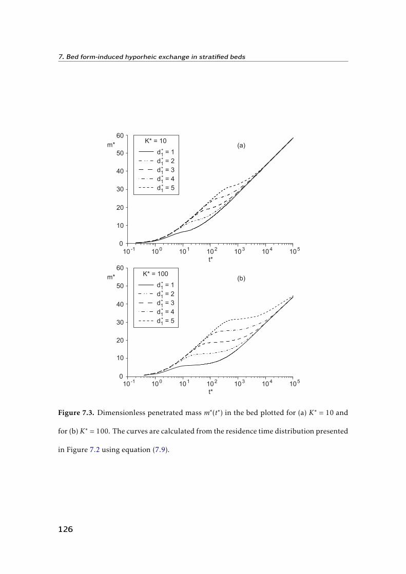
7. Bed form-induced hyporheic exchange in stratified beds
K* = 10
d1 = 1
d1 = 2
d1 = 3
d1 = 4
d1 = 5*
*
*
*
*
K* = 100
d1 = 1
d1 = 2
d1 = 3
d1 = 4
d1 = 5*
*
*
*
*
10-1
100
101
102
103
104
105
0
10
10
20
20
30
30
40
40
50
50
60
60
t*
m*
m*
10-1
100
101
102
103
104
105
0
t*
(a)
(b)
Figure 7.3. Dimensionless penetrated mass m∗(t∗) in the bed plotted for (a) K∗ = 10 and
for (b)K∗ = 100. The curves are calculated from the residence time distribution presented
in Figure 7.2 using equation (7.9).
126

7.3 Experiments
ment was placed in the channel and a constant volume of water was continuously
recirculated over the bed.
Sodium chloride (NaCl) was used as a conservative tracer to evaluate mass
transfer from the overlying flow to the pore water. A concentrated NaCl solution
was prepared using reagent-grade salt and then added to the downstream end of
the flume over one recirculation period in order to establish a uniform salt con-
centration in the stream. The surface-subsurface exchange flux was determined
from the rate of change of the in-stream concentration by considering the mass
balance between the recirculation stream and the pore water in the sediment bed.
Seven tests were performed to observe exchange with different sediment struc-
tures under different flow conditions. Four experiments (Exp. 1–3, 5) were per-
formed with flat beds having different subsurface structure and will not be con-
sidered here. The reader is invited to read the paper by Marion et al. (2008a) for
a complete description of the tests and the relevant results.
Three tests (Exp. 4, 6 and 7) were performed with stationary bed forms, and
had both layered and homogeneous sediment structure. The bed forms were
formed manually to approximate a natural dune shape and had a wavelength
λ = 50cm and a height of H = 5cm. In Experiments 4 and 6, the sediment struc-
ture was layered, with a 3cm-thick layer of gravel overlying a 12cm-thick layer of
a sand-gravel mixture with bed forms formed in the gravel layer. The sand-gravel
mixture was composed of 50% pea gravel and 50% coarse sand. The pea gravel
had a relatively narrow distribution with diameters D10 = 2mm, D50 = 6mm,
D90 = 9mm. The mean bulk porosity of the clean gravel was θ = 0.38. The sand
had D10 = 0.2mm, D50 = 0.8mm and D90 = 2mm and also had a porosity of ap-
proximately 0.38. The composition of the gravel and the sand-gravel mixture is
shown in Figure 7.4.
Exp. 4 had a mean overlying velocity U = 0.36ms−1 while Exp. 6 had a mean
overlying velocity U = 0.21ms−1. Exp. 7 was conducted with the sand-gravel
127
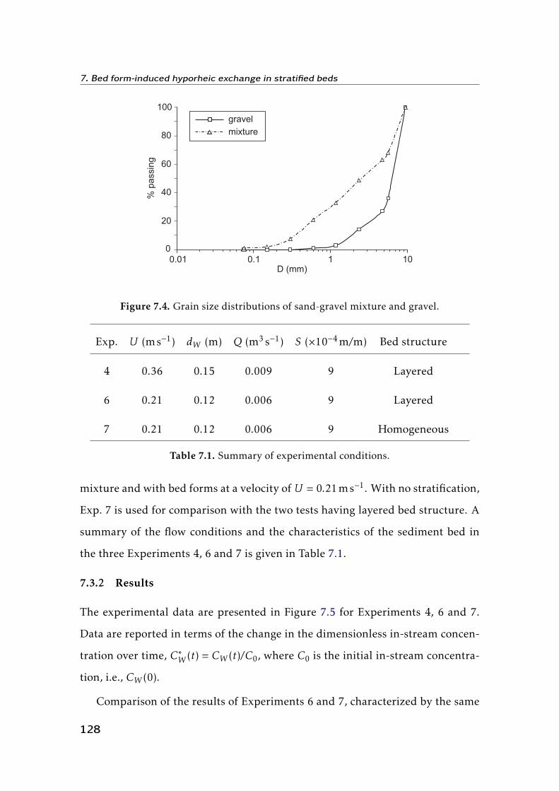
7. Bed form-induced hyporheic exchange in stratified beds
gravel
mixture
0
20
40
60
80
100
0.01 0.1 1 10D (mm)
% p
assin
g
Figure 7.4. Grain size distributions of sand-gravel mixture and gravel.
Exp. U (ms−1) dW (m) Q (m3 s−1) S (×10−4 m/m) Bed structure
4 0.36 0.15 0.009 9 Layered
6 0.21 0.12 0.006 9 Layered
7 0.21 0.12 0.006 9 Homogeneous
Table 7.1. Summary of experimental conditions.
mixture and with bed forms at a velocity ofU = 0.21ms−1. With no stratification,
Exp. 7 is used for comparison with the two tests having layered bed structure. A
summary of the flow conditions and the characteristics of the sediment bed in
the three Experiments 4, 6 and 7 is given in Table 7.1.
7.3.2 Results
The experimental data are presented in Figure 7.5 for Experiments 4, 6 and 7.
Data are reported in terms of the change in the dimensionless in-stream concen-
tration over time, C∗W (t) = CW (t)/C0, where C0 is the initial in-stream concentra-
tion, i.e., CW (0).
Comparison of the results of Experiments 6 and 7, characterized by the same
128
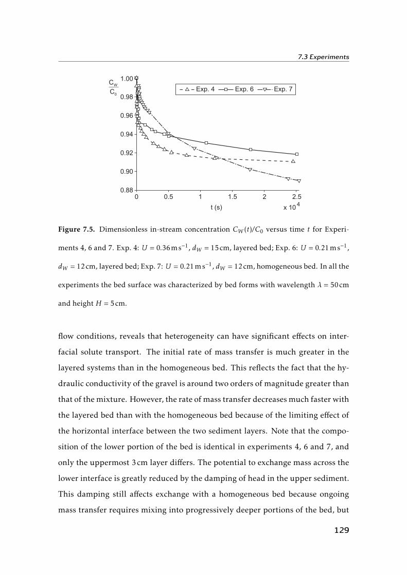
7.3 Experiments
W
0
C
C
0 0.5 1 1.5 2 2.5
x 104
t (s)
0.88
0.90
0.92
0.94
0.96
0.98
1.00
Exp. 4 Exp. 6 Exp. 7
Figure 7.5. Dimensionless in-stream concentration CW (t)/C0 versus time t for Experi-
ments 4, 6 and 7. Exp. 4: U = 0.36ms−1, dW = 15cm, layered bed; Exp. 6: U = 0.21ms−1,
dW = 12cm, layered bed; Exp. 7: U = 0.21ms−1, dW = 12cm, homogeneous bed. In all the
experiments the bed surface was characterized by bed forms with wavelength λ = 50cm
and height H = 5cm.
flow conditions, reveals that heterogeneity can have significant effects on inter-
facial solute transport. The initial rate of mass transfer is much greater in the
layered systems than in the homogeneous bed. This reflects the fact that the hy-
draulic conductivity of the gravel is around two orders of magnitude greater than
that of the mixture. However, the rate of mass transfer decreases much faster with
the layered bed than with the homogeneous bed because of the limiting effect of
the horizontal interface between the two sediment layers. Note that the compo-
sition of the lower portion of the bed is identical in experiments 4, 6 and 7, and
only the uppermost 3cm layer differs. The potential to exchange mass across the
lower interface is greatly reduced by the damping of head in the upper sediment.
This damping still affects exchange with a homogeneous bed because ongoing
mass transfer requires mixing into progressively deeper portions of the bed, but
129
7. Bed form-induced hyporheic exchange in stratified beds
the rate of decrease is greater with a layered bed due to the deflection of the flow
paths at the interface induced by the lower conductivity of the underlying layer.
This is the source of the effective anisotropy that has previously been observed to
limit vertical penetration in heterogeneous beds (Salehin et al., 2004). The over-
all result is that the rate of mass exchange with the homogeneous bed becomes
greater than with layered beds at long times, as can be seen from the crossing
of the curves in Figure 7.5. Comparison of Exp. 4, where U = 0.36ms−1, with
Exp. 6, where U = 0.21ms−1, shows that the increase of velocity induces an in-
crease of mass transfer and the upper layer becomes saturated more rapidly. This
is an expected result since the exchange rates normally increase as the square of
the overlying velocity, as shown by Packman et al. (2004).
7.4 Comparison between model and experimental results
The exchange mass can be evaluated from the in-stream concentration history
using the following relationship for the mass balance of solute in the system:
m∗ = d∗W (1−CW ) . (7.10)
The parameter d∗W is the dimensionless effective water depth, equal to 2πkd′W /θ1,
where d′W is the ratio between the total recirculating volume of water and the bed
surface area.
The hydraulic conductivity used to model hyporheic exchange was evaluated
with the following empirical relation (McCarthy, 2006):
K = 0.35D215 . (7.11)
where hydraulic conductivity, K , has units of cms−1 and D15 is in cm. The hy-
draulic conductivity was evaluated to be K = 3 × 10⁻⁴ ms−1 for the sand-gravel
mixture and K = 0.002ms−1 for gravel only.
130

7.4 Comparison between model and experimental results
The half-amplitude hm of the sinusoidal dynamic head over bed forms was
evaluated with Felhman (1985) equation:
hm = 0.28U2
2g×
(H/d0.34
3/8), H/dW ≤ 0.34 ,(
H/d0.34
3/2), H/dW > 0.34 ,
(7.12)
where H is the bed form height (through-to-crest). In Experiments 6 and 7
the half-amplitude of the dynamic head predicted by equation (7.12) is hm =
0.85mm, while in Exp. 4 it is hm = 2.51mm.
The observed and predicted mass transfer for Experiments 4 and 6 are com-
pared in Figure 7.6. A linear time scale is used in Figure 7.6a, while a semi-log
scale is used in Figure 7.6b for direct comparison with Figure 7.3. The scatter of
data at short times is to be attributed to the difficulty of the advective model to
represent in detail the complex interactions affecting early transfer at flow/bed
interface. These tests both had bed forms and layered sediment structure, with
K∗ = 67, d∗1 and d∗2 = 1.51, but different overlying velocities. The collapse of data
from the two tests onto a single unique curve shows that the scalings used to
non-dimensionalize mass transfer and time are correct. Thus, the scaling of the
exchange rate with U2 still holds even with the heterogeneous bed. The first
phase of the exchange is fast and governed by the 3cm-deep upper layer. The in-
flection point of the curve corresponds to the time at which the upper permeable
layer becomes saturated with solute. After this time the exchange process is gov-
erned by mass transfer into the lower and less permeable layer. Therefore it can
be seen that the initial phase of mass transfer is regulated by the characteristics
of the surficial sediment layer, while tracer exchange rate over longer timescales
depends on the characteristics of the underlying less permeable material.
131

7. Bed form-induced hyporheic exchange in stratified beds
(b)
(a)
0
2
4
6
8m
*
Exp. 6Exp. 4 model
0 50 100 150 200
t*
Exp. 6Exp. 4 model
t*1 10 100
0
2
4
6
8
m*
Figure 7.6. Observed and predicted dimensionless penetrated mass m∗(t∗) for Exp. 4 and
Exp. 6 plotted in (a) linear scale and (b) semi-log sclae. In both experiments the bed
was made of two horizontal layers with artificial bed forms at the flow/bed interface.
The difference between the two tests was the mean flow velocity and the water depth, as
reported in Table 7.1.
132

7.5 Conclusions
7.5 Conclusions
A mathematical model was developed for the pore water flow induced in a lay-
ered sediment bed by the dynamic pressure variation over dune-shaped bed forms.
For the case of a coarser surface layer over a finer and less permeable layer, the
flow paths in the upper layer are compressed by the presence of the underly-
ing low permeability layer thus suppressing mass transfer into the lower layer. A
comparison of exchange with homogeneous and layered beds shows that the pres-
ence of a coarse near-surface layer increases the interfacial flux and initial rate of
mass transfer, but decreases vertical solute penetration into the underlying finer
sediments and the corresponding net mass transfer at longer time scales.
These results emphasize the importance of sediment structure on surface-
subsurface flow coupling and solute exchange. The presence of deeper layers
of differing permeability, which are often found in rivers because of episodic sed-
iment transport events (Leopold et al., 1964), causes rates of mass transfer into
the bed to vary over time as solute penetrates to the different layers of sediments.
When such systems are analyzed using a model that assumes homogeneous sub-
surface structure, the instantaneous exchange rate will be overestimated and
underestimated at different stages of the overall exchange process. The results
and theoretical analysis presented here support the recommendation previously
made by other authors (Harvey and Wagner, 2000; Zaramella et al., 2003) that it is
important to combine observations of tracer concentration in surface waters with
characterization of the subsurface structure and direct observations of tracer pen-
etration to particular depths of interest.
133


Notation
The symbols and notation appearing in this thesis are listed below. Within the
main body of the text, symbols are usually defined at their first usage within a
chapter, or at other times when needed for clarity. In some cases equations have
been presented using the same notation used in the original papers; in other
cases, original notation has been altered to better fit with the surrounding mate-
rial.
Acronyms
ADE Advection-Dispersion Equation;
APM Advective Pumping Model;
BTC Breakthrough Curve;
CTRW Continuous Time Random Walk;
FADE Fractional Advection Dispersion Equation;
GME Generalized Master Equation;
MRMT Multi-Rate Mass Transfer;
PDF Probability Density Function;
RMSE Root Mean Square Error;
RTD Residence Time Distribution;
RWT Rodhamine-WT;
STIR Solute Transport In Rivers;
135
Notation
TSM Transient Storage Model.
Roman symbols
Upper case
A average stream cross-sectional area [L2];
AS average cross-sectional area of storage zones [L2];
C concentration [ML−3];
C∗ dimensionless concentration, C∗ = C/C0 [ - ];
C0 reference concentration [ML−3];
CADδ solution of conventional advection-dispersion equation for an input mass
pulse [ML−3];
CL concentration of solute in lateral inflow [ML−3];
Cobs observed concentration [ML−3];
CS concentration of solute in the sediments [ML−3];
Csim simulated concentration [ML−3];
CW concentration in the main channel [ML−3];
CWδ impulsive solution for the concentration in the main channel [ML−3]
D10 grain size for which 10% by weight of the sediment is finer [L];
D50 grain size for which 50% by weight of the sediment is finer [L];
D90 grain size for which 90% by weight of the sediment is finer [L];
Dε dispersion coefficient of fractional advection-dispersion equation [L2 T−1];
Dm molecular diffusion coefficient [L2 T−1];
DL longitudinal dispersion coefficient [L2 T−1];
DS diffusion coefficient in the porous medium of the diffusive transport model
[L2 T−1];
Dij components of the dispersion tensor of the porous medium [L2 T−1];
DTij components of the turbulent dispersion tensor [L2 T−1];
F F-value of F-test of the overall linear fit [- ];
136

Notation
H bed form height [L];
I set of observed concentration values, I = IU ∪ IL ;
IL set of observed concentration values lower than a given threshold concen-
tration;
IU set of observed concentration values higher than a given threshold con-
centration;
K hydraulic conductivity of the porous bed [LT−1];
K∗ ratio of conductivities of upper and lower sediment layer, K∗ = K1/K2 [ - ];
K1 hydraulic conductivity of the upper sediment layer [LT−1];
K2 hydraulic conductivity of the lower sediment layer [LT−1];
L length of study reach [L];
Lmix distance from injection at which a solute can be considered well-mixed
over the cross-section [L];
M0 injected mass [M];
MS retained mass [M];
P wetted perimeter [L];
P0 probability of rejecting, when true, the null hypothesis that the angular
coefficient of linear regression is zero [- ];
Q flow discharge [L3 T−1];
R complementary cumulative residence time distribution [- ];
R0 complementary cumulative distribution of the residence time within the
bed induced by advective pumping in the ideal case of stream gradient
and bed form propagation celerity equal to zero [- ];
Rad retardation factor due to reversible adsorption onto sediments [- ];
R2det coefficient of determination [- ];
S stream gradient [- ];
T residence timescale [T];
TB residence timescale in the hyporheic zone [T];
137
Notation
TD residence timescale in the surface dead zones [T];
U average flow velocity [LT−1]
Ub celerity of moving bed forms [LT−1];
U ∗b dimensionless celerity of moving bed forms, U ∗b = θUb/um [ - ];
U ∗uf dimensionless magnitude of relative underflow velocity [- ].
Lower case
b channel width [L];
c local instantaneous concentration [ML−3];
c time average of the local instantaneous concentration [ML−3];
dW water depth [L];
d average depth of the hyporheic zone [L];
d∗ average dimensionless depth of the hyporheic zone, d∗ = kd [ - ];
d1 thickness of the upper sediment layer [L]
d2 thickness of the lower sediment layer [L]
eMS residuals from a linear model explaining δMS,max as a function chlorophyll-
a [M];
fM memory function [T−1];
h dynamic head [L];
h∗ dimensionless dynamic head, h∗ = h/hm [ - ];
h∗12 dimensionless semi-amplitude of the dynamic head at the interface be-
tween the upper and lower layer [- ];
hm semi-amplitude of the dynamic head on the bed surface [L];
m accumulated mass in the bed per unit plan area of stream divided by a
reference concentration C0 [L];
m∗ dimensionless penetrated mass, m∗ = 2πkm/θ [ - ];
pα probability density function of first-order coefficients [T];
pi conditional probability distribution of the random variableNi [ - ];
138

Notation
q average volumetric flux across the stream-subsurface interface [LT−1];
q∗ dimensionless volumetric average flux across the stream-subsurface inter-
face [LT−1];
qB average volumetric flux in the hyporheic zones [LT−1];
qL volumetric flux due to lateral inflow [LT−1];
rW probability density function (PDF) of the residence time the surface water,
TW [T−1];
rS probability density function (PDF) of the overall residence time in the
storage zones, TS [T−1];
rSi probability density function (PDF) of the overall residence time in the i-th
storage domain, TSi [T−1];
rSi |n conditional residence time probability density function (PDF) in the i-th
storage domain given that a particle has entered the storage domain n
times [T−1];
s Laplace variable [T−1];
t time [T];
t averaging timescale [T];
t∗ dimensionless time [- ];
tad average advection time, tad = L/U [T];
tB biofilm age [T];
tc cutoff time scale of advective pumping-induced power-law behavior [T];
t∗c dimensionless cutoff time scale of advective pumping-induced power-law
behavior [- ];
td time scale of exponential decay [T];
t∗d dimensionless time scale of exponential decay [- ];
u velocity vector, u = (u,v,w) [LT−1];
u time average of velocity field, u = (u,v,w) [LT−1];
u∗ dimensionless velocity field, u∗ = (u∗,v∗,w∗) [ - ];
139

Notation
u∗ shear velocity [LT−1];
um maximum pumping-induced velocity, um = kKhm [LT−1];
us seepage velocity induced by the stream gradient [LT−1];
u∗s dimensionless seepage velocity induced by the stream gradient [- ];
x position vector, x = (x,y,z) [L];
x∗ dimensionless position vector, x∗ = kx = (x∗, y∗, z∗) [ - ];
zchla z-standardized value of chlorophyll-a [ - ].
Calligraphic symbols
Ni number of times a particle enters the i-th storage domain (random vari-
able) [ - ];
T total residence time in the study reach (random variable) [T];
TS overall residence time in the storage zones (random variable) [T];
TSi overall residence time in the i-th storage domain (random variable) [T];
TW residence time in the surface water (random variable) [T].
Greek symbols
Upper case
ΓS source/sink term of advection-dispersion-mass-transfer equation [ML−3 T−1];
∆tinj time length of injection period [T];
Φ mass flux [ML−2 T−1];
ΦL mass flux accounting for mass gains due to lateral inflow [ML−2 T−1];
ΦS mass flux into the storage zones [ML−2 T−1];
Ψ joint probability density function of length and duration of particle
jumps [L−1 T−1].
140

Notation
Lower case
α transfer rate [T−1];
αL longitudinal dispersivity [L];
α∗L dimensionless longitudinal dispersivity, α∗L = kαL [ - ];
αT transverse dispersivity [L];
α∗T dimensionless transverse dispersivity, α∗T = kαT [ - ];
βtot capacity coefficient [- ];
δα transfer rate associated to biofilm-induced retention [T−1];
δMS increment of retained mass [M];
δϕ residence time PDF associated to biofilm-induced retention [T−1];
δMS,max peak of increment of retained mass [M];
ε order of fractional derivative [- ];
θ porosity of the porous medium [-];
θ1 porosity of the upper sediment layer [- ];
κ exponent of power-law RTD [-];
λ bed form wavelength [L];
λc horizontal distance between the crest and the upstream trough of a bed
form [L];
ν(s) composite Laplace variable [T−1];
ς skewness coefficient of fractional advection-dispersion equation [- ];
ϕ probability density function (PDF) of the residence time in the storage
zones for a single entry event [T−1];
ϕ0 PDF of the residence time within the bed for advective pumping in the
ideal case of stream gradient and bed form propagation celerity equal
to zero [T−1];
ϕi probability density function (PDF) of the residence time in the i-th stor-
age domain for a single entry [T−1];
141

Notation
ϕB probability density function (PDF) of the residence time in the hyporheic
zone for a single entry [T−1];
ϕD probability density function (PDF) of the residence time in the surface
dead zones fora single entry [T−1];
ψL probability density function (PDF) of the length of particle jumps [L−1];
ψT probability density function (PDF) of the duration of particle jumps
[T−1];
ψT 0 probability density function (PDF) of the duration of particle jumps in
the absence of retention processes [T−1].
142
Bibliography
Battin, T. J., L. A. Kaplan, J. D. Newbold, and C. M. E. Hansen (2003), Contribu-
tions of microbial biofilms to ecosystem processes in stream mesocosms, Na-
ture, 426(6965), 439–442.
Battin, T. J., L. A. Kaplan, S. Findlay, C. S. Hopkinson, E. Marti, A. I. Packman,
J. D. Newbold, and F. Sabater (2008), Biophysical controls on organic carbon
fluxes in fluvial networks, Nature Geosci., 1(2), 95–100.
Bencala, K. E. (1984), Interactions of solutes and streambed sediment. II. A dy-
namic analysis of coupled hydrologic and chemical processes that determine
solute transport, Water Resour. Res., 20(12), 1804–1814.
Bencala, K. E., and R. A. Walters (1983), Simulation of solute transport in a moun-
tain pool-and-riffle stream: A transient storage model, Water Resour. Res., 19(3),
718–724.
Benekos, D. I. (2005), On the determination of transverse dispersivity: Experi-
ments and simulations in a helix and a cochlea, Ph.D. diss., Dept. of Civil and
Environ. Eng., Standford Univ., Standford (CA).
Berkowitz, B., and H. Scher (1995), On characterization of anomalous dispersion
in porous and fractured media, Water Resour. Res., 31(6), 1461–1466.
143
Bibliography
Besemer, K., G. Singer, R. Limberger, A. Chlup, G. Hochedlinger, I. Hodl,
C. Baranyi, and T. J. Battin (2007), Biophysical controls on community suc-
cession in stream biofilms, Appl. Environ. Microbiol., 73(15), 4966–4974.
Blank, L. (1996), Numerical treatment of differential equations of frac-tional or-
der, Tech. Rep. 287, Manchester Centre for Computational Mathematics Nu-
merical Analysis.
Boano, F., C. Camporeale, R. Revelli, and L. Ridolfi (2006a), Sinuosity-driven
hyporheic exchange in meandering rivers, Geophys. Res. Lett., 33, L18,406.
Boano, F., R. Revelli, and L. Ridolfi (2006b), Bedform-induced hyporheic ex-
change with unsteady flow, Geophys. Res. Lett., 30(1), 148–156.
Boano, F., A. I. Packman, A. Cortis, R. Revelli, and L. Ridolfi (2007), A continuous
time random walk approach to the stream transport of solutes, Water Resour.
Res., 43, W10,425.
Boano, F., R. Revelli, and L. Ridolfi (2008), Reduction of the hyporheic zone vol-
ume due to the stream-aquifer interaction, Geophys. Res. Lett., 35, L09,401.
Briggs, M. A., M. N. Gooseff, C. D. Arp, and M. A. Baker (2009), A method for
estimating surface transient storage parameters for streams with concurrent
hyporheic storage, Water Resour. Res., 45, W00D27.
Brinkman, H. C. (1949), A calculation of the viscous force exerted by a flowing
fluid on a dense swarm of particles, App. Sci. Res., 1(1), 27–34.
Calhoun, D., and R. J. LeVeque (2000), A cartesian grid Finite-Volume method
for the Advection-Diffusion equation in irregular geometries, J. Comput. Phys.,
157(1), 143–180.
Cardenas, M. B. (2003), Three-dimensional model of modern channel bend de-
posits, Water Resour. Res., 19(6), 1141.
144

Bibliography
Cardenas, M. B., and J. L. Wilson (2006), The influence of ambient groundwa-
ter discharge on exchange zones induced by current-bedform interactions, J.
Hydrol., 331(1-2), 103–109.
Cardenas, M. B., and J. L. Wilson (2007), Dunes, turbulent eddies, and interfacial
exchange with permeable sediments, Water Resour. Res., 43, W08,412.
Cardenas, M. B., J. L. Wilson, and V. A. Zlotnik (2004), Impact of heterogeneity,
bed forms, and stream curvature on subchannel hyporheic exchange, Water
Resour. Res., 40, W08,307.
Carrera, J., X. SÃąnchez-Vila, I. Benet, A. Medina, G. Galarza, and J. GuimerÃă
(1998), On matrix diffusion: formulations, solution methods and qualitative
effects, Hydrogeol. J., 6(1), 178–190.
Castro, N. M., and G. M. Hornberger (1991), Surface-subsurface interactions in
an alluviated mountain stream channel, Water Resour. Res., 27(7), 1613–1621.
Chaves, A. S. (1998), A fractional diffusion equation to describe Lévy flights,
Phys. Lett. A, 239(1-2), 13–16.
Choi, J., S. M. Hulseapple, M. H. Conklin, and J. W. Harvey (1999), Modeling CO2
degassing and pH in a stream-aquifer system, J. Hydrol., 209(1-4), 297–310.
Choi, J., J. W. Harvey, and M. H. Conklin (2000), Characterizing multiple
timescales of stream and storage zone interaction that affect solute fate and
transport in streams, Water Resour. Res., 36(6), 1511–1518.
Colbeck, S. C. (1989), Air movement in snow due to wind-pumping, J. Glaciol.,
35(120), 209âĂŞ213.
Cortis, A., T. Harter, L. L. Hou, E. R. Atwill, A. I. Packman, and P. G. Green (2006),
Transport of cryptosporidium parvum in porous media: Long-term evolution
145

Bibliography
experiments and continuous time random walk filtration modeling, Water Re-
sour. Res., 42(12), W12S13.
Czernuszenko, W., and P. M. Rowinski (1997), Properties of the dead zone model
of longitudinal dispersion in rivers, J. Hydraul. Res., 35(4), 491–504.
Day, T. J. (1975), Longitudinal dispersion in natural channels, Water Resour. Res.
De Smedt, F. (2006), Analytical solutions for transport of decaying solutes in
rivers with transient storage, J. Hydrol., 330(3-4), 672–680.
De Smedt, F., and P. J. Wierenga (2005), Analytical solution for solute transport
resulting from instantaneous injection in streams with transient storage, J. Hy-
drol., 315(1-4), 25–39.
DeAngelis, D. L., M. Loreau, D. Neergaard, P. J. Mulholland, and E. R. Marzolf
(1995), Modelling nutrient-periphyton dynamics in streams: the importance of
transient storage zones, Ecol. Model., 80(2-3), 149–160.
Deng, Z.-Q., V. P. Singh, and L. Bengtsson (2004), Numerical solution of frac-
tional advection-dispersion equation, J. Hydraul. Eng., 130(5), 422–431.
Deng, Z.-Q., L. Bengtsson, and V. P. Singh (2006), Parameter estimation for frac-
tional dispersion model for rivers, Environ. Fluid. Mech., 6(5), 451–475.
Dent, C. L., and J. C. Henry (1999), Modelling nutrient-periphyton dynamics in
streams with surface-subsurface exchange, Ecol. Model., 122(1-2), 97–116.
Dierberg, F. E., and T. A. DeBusk (2005), An evaluation of two tracers in suface-
flow wetlands: Rhodamine-WT and lithium, Wetlands, 25(1), 8–25.
Elder, J. W. (1959), The dispersion of marked fluid in turbulent shear flow, J.
Fluid. Mech., 5(04), 544–560.
146
Bibliography
Elliott, A. H., and N. H. Brooks (1997a), Transfer of nonsorbing solutes to a
streambed with bed forms: Theory, Water Resour. Res., 33(1), 123–136.
Elliott, A. H., and N. H. Brooks (1997b), Transfer of nonsorbing solutes to a
streambed with bed forms: Laboratory experiments, Water Resour. Res., 33(1),
137–151.
Felhman, H. S. (1985), Resistance components and velocity distributions of open
channel flows over bedforms, Master’s thesis, Colorado State University, Fort
Collins, Colorado.
Fernald, A. G., P. J. Wigington, and D. H. Landers (2001), Transient storage and
hyporheic flow along the Willamette River, Oregon: Field measurements and
model estimates, Water Resour. Res., 37(6), 1681–1694.
Fick, A. (1855), Annln. Phys., 170, 59.
Fischer, H. B. (1968), Dispersion prediction in natural streams, J. Sanit. Eng. Div.,
ASCE, 94(5), 927–943.
Fischer, H. B. (1975), Discussion of "Simple method for predicting dispersion in
streams", J. Env. Eng. Div., ASCE, 101(3), 435–455.
Fischer, H. B., J. E. List, C. R. Koh, J. Imberger, and N. H. Brooks (1979), Mixing
in Inland and Coastal Waters, Academic Press.
Gooseff, M. N., D. M. McKnight, R. L. Runkel, and B. H. Vaughn (2003a), Deter-
mining long time-scale hyporheic zone flow paths in Antarctic streams, Hydrol.
Process., 17(9), 1691–1710.
Gooseff, M. N., S. M. Wondzell, R. Haggerty, and J. Anderson (2003b), Comparing
transient storage modeling and residence time distribution (RTD) analysis in
geomorphically varied reaches in the lookout creek basin, oregon, USA, Adv.
Water. Resour., 26(9), 925–937.
147
Bibliography
Gooseff, M. N., D. M. McKnight, R. L. Runkel, and J. H. Duff (2004), Denitrifica-
tion and hydrologic transient storage in a glacial meltwater stream, McMurdo
dry valleys, antarctica, Limnol. Oceanogr., 49(5), 1884–1895.
Gooseff, M. N., J. LaNier, R. Haggerty, and K. Kokkeler (2005), Determining
in-channel (dead zone) transient storage by comparing solute transport in a
bedrock channel-alluvial channel sequence, Oregon, USA, Water Resour. Res.,
41, W06014.
Gooseff, M. N., R. O. H. Jr., and J. L. Tank (2007), Relating transient storage to
channel complexity in streams of varying land use in jackson hole, wyoming,
Water Resour. Res., 43, W01,417.
Haggerty, R., and S. M. Gorelick (1995), Multiple-Rate mass transfer for modeling
diffusion and surface reactions in media with Pore-Scale heterogeneity, Water
Resour. Res., 31(10), 2383–2400.
Haggerty, R., and S. M. Wondzell (2002), Power-law residence time distribution in
the hyporheic zone of a 2nd-order mountain stream, Geophys. Res. Lett., 29(13),
1640.
Haggerty, R., S. A. McKenna, and L. C. Meigs (2000), On the late-time behavior
of tracer test breakthrough curves, Water Resour. Res., 36(12), 3467–3479.
Hall Jr., R. O., E. S. Bernhardt, and G. E. Likens (2002), Relating nutrient uptake
with transient storage in forested mountain streams, Limnol. Oceanogr., 47(1),
255–265.
Hart, D. R. (1995), Parameter estimation and stochastic interpretation of the tran-
sient storage model for solute transport in streams, Water Resour. Res., 31(2),
323–328.
148
Bibliography
Harvey, J. W., and K. E. Bencala (1993), The effect of streambed topography
on Surface-Subsurface water exchange in mountain catchments, Water Resour.
Res., 29(1), 89–98.
Harvey, J. W., and C. C. Fuller (1998), Effect of enhanced manganese oxidation
in the hyporheic zone on basin-scale geochemical mass balance, Water Resour.
Res., 34(4), 623–636.
Harvey, J. W., and B. J. Wagner (2000), Quantifying hydrologic interactions be-
tween streams and their subsurface hyporheic zones, in Streams and Groundwa-
ter, edited by J. B. Jones and P. J. Mulholland, pp. 3–44, Academic, Sand Diego
(CA).
Harvey, J. W., B. J. Wagner, and K. E. Bencala (1996), Evaluating the reliability of
the stream tracer approach to characterize stream-subsurface water exchange,
Water Resour. Res., 32(8), 2441–2451.
Harvey, J. W., J. E. Saiers, and J. T. Newlin (2005), Solute transport and storage
mechanisms in wetlands of the everglades, south florida, Water Resour. Res., 41,
W05,009.
Hays, J. R., P. A. Krenkel, and K. B. J. Schnelle (1966), Mass transport mechanism
in open channel flow, Tech. Rep. 8, Vanderbilt University, Nashville, Tennessee.
Jackman, A., R. Walters, and V. Kennedy (1984), Transport and concentration
controls for chloride, strontium, potassium and lead in uvas creek, a small
cobble-bed stream in santa clara county, california, U.S.A.: 2. Mathematical
modeling, J. Hydrol., 75(1-4), 111–141.
Johansson, H., K. Jonsson, K. J. Forsman, and A. Wörman (2001), Retention of
conservative and sorptive solutes in streams – Simultaneous tracer experiment,
Sci. Total. Environ., 266(1-3), 229–238.
149

Bibliography
Jonsson, K., H. Johansson, and A. Wörman (2003), Hyporheic exchange of re-
active and conservative solutes in streams – Tracer methodology and model
interpretation, J. Hydrol., 278(1-4), 151–169.
Jonsson, K., H. Johansson, and A. Wörman (2004), Sorption behaviour and long-
term retention of reactive solutes in the hyporheic zone of streams, J. Eniviron.
Eng., 130(5), 573–584.
Kim, B. K., A. I. Packman, and F. J. Triska (1990), Modeling transient storage and
nitrate uptake kinetics in a flume containing a natural periphyton community,
Water Resour. Res., 26(3), 505–515.
Kim, B. K. A., A. P. Jackman, and F. J. Triska (1992), Modeling biotic uptake
by periphyton and transient hyporrheic storage of nitrate in a natural stream,
Water Resour. Res., 28(10), 2743–2752.
Kim, S., and M. L. Kavvas (2006), Generalized Fick’s law and fractional ADE for
pollution transport in a river: Detailed derivation, J. Hydraul. Eng., 11(1), 80–
83.
Krenkel, P. A., and G. T. Orlob (1962), Turbulent diffusion and the reaereation
coefficient, J. Sanit. Eng. Div., ASCE, 88(SA2), 3079.
Lees, M. J., L. A. Camacho, and S. C. Chapra (2000), On the relationship of tran-
sient storage and aggregated dead zone models of longitudinal solute transport
in streams., Water Resour. Res., 36(1), 213–224.
Leopold, L. B., M. G. Wolman, and J. P. Miller (1964), Fluvial processes in geomor-
phology, Freeman and Co., San Francisco (CA).
LeVeque, R. J. (1997), Wave propagation algorithms for multidimensional hyper-
bolic systems, J. Comput. Phys., 131(2), 327–353.
150

Bibliography
Margolin, G., and B. Berkowitz (2000), Application of continuous time random
walks to transport in porous media, J. Phys. Chem., 104(16), 3942–3947, erra-
tum: 104(36), 8762, 2000.
Margolin, G., M. Dentz, and B. Berkowitz (2003), Continuous time random walk
and multirate mass transfer modeling of sorption, Chem. Phys., 295(1), 71–80.
Marion, A., and M. Zaramella (2005a), Diffusive behavior of bedform-induced
hyporheic exchange in rivers, J. Eniviron. Eng., 131(9), 1260–1266.
Marion, A., and M. Zaramella (2005b), A residence time model for stream-
subsurface exchange of contaminants, Acta Geophysica Polonica, 53(4), 527.
Marion, A., and M. Zaramella (2006), Effects of velocity gradients and secondary
flow on the dispersion of solutes in a meandering channel, J. Hydraul. Eng.,
132(12), 1295–1302.
Marion, A., M. Bellinello, I. Guymer, and A. I. Packman (2002), Effect of bed form
geometry on the penetration of nonreactive solutes into a streambed, Water
Resour. Res., 38(10), 1209.
Marion, A., M. Zaramella, and A. I. Packman (2003), Parameter estimation of the
transient storage model for stream-subsurface exchange, Water Resour. Res.,
129(5), 456–463.
Marion, A., A. I. Packman, M. Zaramella, and A. Bottacin-Busolin (2008a), Hy-
porheic flows in stratified beds, Water Resour. Res., 44, W09,433.
Marion, A., M. Zaramella, and A. Bottacin-Busolin (2008b), Solute transport in
rivers with multiple storage zones: The STIR model, Water Resour. Res., 44,
W10,406.
McCarthy, D. F. (2006), Essentials of Soil Mechanics and Foundations: Basic Geotech-
nics, 7 ed., Prentice Hall.
151

Bibliography
Metzler, R., and J. Klafter (2000), Subdiffusive transport close to thermal equilib-
rium: from the Langevin equation to fractional diffusion, Phys. Rev. E, 61(6),
6308–6311.
Montroll, E. W., and G. H. Weiss (1965), Random walks on lattices, J. Math. Phys.,
6, 167–181.
Mulholland, P. J., A. D. Steinman, E. R. Marzolf, D. R. Hart, and D. L. DeAngelis
(1994), Effect of periphyton biomass on hydraulic characteristics and nutrient
cycling in streams, Oecologia, 98(1), 40–47.
Mulholland, P. J., E. R. Marzolf, J. R. Webster, D. R. Hart, and S. P. Hendricks
(1997a), Evidence that hyporheic zones increase hetrotrophic metabolism and
phosphorus uptake in forest streams, Limnol. Oceanogr., 42, 443–451.
Mulholland, P. J., E. R. Marzolf, J. R. Webster, D. R. Hart, and S. P. Hendricks
(1997b), Evidence that hyporheic zones increase heterotrophic metabolism and
phosphorus uptake in forest streams, Limnology and Oceanography, 42(3), 443–
451.
Mulholland, P. J., A. M. Helton, G. C. Poole, R. O. Hall, S. K. Hamilton, B. J.
Peterson, J. L. Tank, L. R. Ashkenas, L. W. Cooper, C. N. Dahm, W. K. Dodds,
S. E. G. Findlay, S. V. Gregory, N. B. Grimm, S. L. Johnson, W. H. McDowell,
J. L. Meyer, H. M. Valett, J. R. Webster, C. P. Arango, J. J. Beaulieu, M. J. Bernot,
A. J. Burgin, C. L. Crenshaw, L. T. Johnson, B. R. Niederlehner, J. M. O/’Brien,
J. D. Potter, R. W. Sheibley, D. J. Sobota, and S. M. Thomas (2008), Stream
denitrification across biomes and its response to anthropogenic nitrate loading,
Nature, 452(7184), 202–205.
Nagaoka, H., and A. J. Ohgaki (1990), Mass transfer mechanism in a porous
riverbed, Water Resour., 24(4), 417–425.
152

Bibliography
Nordin, C. F., and G. V. Sabol (1974), Empirical data on longitudinal dispersion
in rivers, U.S. Geological Survey, pp. 20–74.
Nordin, C. F., and B. M. Troutman (1980), Longitudinal dispersion in rivers: The
persistence of skewness in observed data, Water Resour. Res.
Orr, C. H., J. J. Clark, P. R. Wilcock, J. C. Finlay, and M. W. Doyle (2009), Compar-
ison of morphological and biological control of exchange with storage zones in
a field-scale flume, J. Geophys. Res., 114, G02,019.
Packman, A. I., and N. H. Brooks (2001), Hyporheic exchange of solutes and col-
loids with moving bed forms, Water Resour. Res., 37(10), 2591–2605.
Packman, A. I., N. H. Brooks, and J. J. Morgan (2000a), Kaolinite exchange be-
tween a stream and streambed: Laboratory experiments and validation of a
colloid transport model, Water Resour. Res., 36(8), 2363–2372.
Packman, A. I., N. H. Brooks, and J. J. Morgan (2000b), A physicochemical model
for colloid exchange between a stream and a sand streambed with bed forms,
Water Resour. Res., 36(8), 2351–2361.
Packman, A. I., S. Mashfiqus, and M. Zaramella (2004), Hyporheic exchange with
gravel beds: Basic hydrodynamic interactions and bedform-induced advective
flows, J. Hydraul. Eng., 130(7), 647–656.
Polyanin, A. D. (2002), Handbook of linear partial differential equations for engineers
and scientists, Chapman & Hall/CRC Press.
Price, K. V., R. M. Storn, and J. A. Lampinen (2005), Differential evolution, Natural
Computing Series, Springer.
Qian, Q., V. R. Voller, and H. G. Stefan (2008), A vertical dispersion model for
solute exchange induced by underflow and periodic hyporheic flow in a stream
gravel bed, Water Resour. Res., 44, W07,422.
153
Bibliography
Runkel, R. L. (1998), One-dimensional Transport with Inflow ans Storage (OTIS):
A solute transport model of streams and rivers, US Geol. Surv. Water Resour.
Invest. Rep., pp. 98–4018.
Runkel, R. L., and S. C. Chapra (1993), An efficient numerical solution of the
transient storage equations for solute transport in small streams, Water Resour.
Res., 29(1), 211–215.
Runkel, R. L., D. M. McKnight, K. E. Bencala, and S. C. Chapra (1996), Reac-
tive solute transport in streams 2. simulation of a pH modification experiment,
Water Resour. Res., 32(2), 419–430.
Runkel, R. L., D. M. McKnight, and E. D. Andrews (1998), Analysis of transient
storage subject to unsteady flow: Diel flow variation in an antarctic stream, J.
N. Am. Benthol. Soc., 17(2), 143–154.
Rutherford, J. C. (1994), River Mixing, 1 ed., John Wiley & Sons.
Ryan, R. J., and M. C. Boufadel (2006), Influence of streambed hydraulic con-
ductivity on solute exchange with the hyporheic zone, Environmental Geology,
51(2), 203–210.
Salehin, M., A. I. Packman, and M. Paradis (2004), Hyporheic exchange with het-
erogeneous streambeds: Laboratory experiments and modeling, Water Resour.
Res., 40, W11,504.
Samko, S. G., A. A. Kilbas, and O. I. Marichev (1993), Fractional Integrals and
Derivatives: Theory and Applications, 1 ed., CRC.
Savant, S. A., D. D. Reible, and L. J. Thibodeaux (1987), Convective transport
within stable river sediments, Water Resour. Res., 23(9), 1763–1768.
154
Bibliography
Sawyer, A. H., and M. B. Cardenas (2009), Hyporheic flow and residence time
distributions in heterogeneous cross-bedded sediment, Water Resour. Res., 45,
W08,406.
Scher, H., and M. Lax (1973), Stochastic transport in a disored solid. I. Theory,
Phys. Rev., 137, 4491–4502.
Scher, H., G. Margolin, and B. Berkowitz (2002), Towards a unified framework for
anomalous transport in heterogeneous media, Chem. Phys., 284(1-2), 349–359.
Schumer, R., D. A. Benson, M. M. Meerschaert, and S. W. Wheatcraft (2001), Eule-
rian derivation of the fractional advection-dispersion equation, J. Contaminant.
Hydrol., 48(1), 69–88.
Shimizu, Y., T. Tsujimoto, and H. Nakagawa (1990), Experiment and microscopic
modeling of flow in highly permeable porous medium under free-surface flow,
J. Hydrosci. Hydraul. Eng., 8(1), 69–78.
Sigee, D. C., and D. C. Sigee (2005), Freshwater Microbiology, Wiley.
Smart, P. L., and I. M. S. Laidlaw (1977), An evaluation of some fluorescent dyes
for water tracing, WRR, 13, 15–33.
Storn, R., and K. Price (1997), Differential evolution – a simple and efficient
heuristic for global optimization over continuous spaces, J. Global Optim., 11,
341–359.
Taylor, G. (1954), The dispersion of matter in turbulent flow through a pipe,
Proceedings of the Royal Society of London. Series A. Mathematical and Physical
Sciences, 223(1155), 446–468.
Thackston, E. L., and K. B. J. Schnelle (1970), Predicting effects of dead zones on
stream mixing, J. Sanit. Eng. Div., ASCE, 92(2), 319–331.
155

Bibliography
Thomas, S. A., M. V. H., W. J.R., and M. P.J. (2003), A regression approach to
estimating reactive solute uptake in advective and transient storage zones of
stream ecosystems, Adv. Water. Resour., 26, 965–976.
Tonina, D., and J. M. Buffington (2007), Hyporheic exchange in gravel bed rivers
with pool-riffle morphology: Laboratory experiments and three-dimensional
modeling, Water Resour. Res., 43, W01,421.
Valentine, E. M., and I. R. Wood (1977), Longitudinal dispersion within dead
zones, J. Hydraul. Div. Am. Soc. Civ. Eng., 103, 975âĂŞ1006.
Vallet, H. M., J. A. Morice, C. N. Dahm, and M. E. Campana (1996), Parent
lithology, surface-groundwater exchange, and nitrate retention in headwater
streams, Limnol. Oceanogr., 41(2), 333–345.
van Genuchten, M. T., and P. J. Wierenga (1976), Mass Transfer Studies in Sorbing
Porous Media I. Analytical Solutions, Soil. Sci. Soc. Am. J., 40(4), 473–480.
Wimpenny, J. W., and R. Colasanti (1997), A unifying hypothesis for the structure
of microbial biofilms based on cellular automaton models, FEMS Microbiology
Ecology, 22(1), 1–16.
Wörman, A., A. I. Packman, H. Johansson, and K. Jonsson (2002), Effect of flow-
induced exchange in hyporheic zones on longitudinal transport of solutes in
streams and rivers, Water Resour. Res., 38(1), 1001.
Wörman, A., A. I. Packman, L. Marklund, J. W. Harvey, and S. H. Stone (2006),
Exact three-dimensional spectral solution to surface-groundwater interactions
with arbitrary surface topography, Geophys. Res. Lett., 33, L07,402.
Wörman, A., A. I. Packman, L. Marklund, J. W. Harvey, and S. H. Stone (2007),
Fractal topography and subsurface water flows from fluvial bedforms to the
continental shield, Geophys. Res. Lett., 34, L07,402.
156
Bibliography
Zaramella, M., A. I. Packman, and A. Marion (2003), Application of the transient
storage model to analyze advective hyporheic exchange with deep and shallow
sediment beds, Water Resour. Res., 39(7), 1198.
Zaramella, M., A. Marion, and A. I. Packman (2006), Applicability of the Tran-
sient Storage Model to the hyporheic exchange of metals, J. Contaminant. Hy-
drol., 84(1-2), 21–35.
Zheng, C., and G. D. Bennett (1995), Applied Contaminant Transport Modeling,
John Wiley & Sons, Incorporated, New York.
Zhou, D., and C. Mendoza (1993), Flow through porous bed of turbulent stream,
J. Eng. Mech., 119(2), 365–383.
157


![arXiv:alg-geom/9505009v1 7 May 1995 · Poisson structure. This was achieved by Bottacin [Bn] and Markman [M1], cf. section 6. In the case of the polynomial matrices though, everything](https://static.fdocuments.net/doc/165x107/5c6b7c7409d3f2843d8b9011/arxivalg-geom9505009v1-7-may-1995-poisson-structure-this-was-achieved-by.jpg)