Transport of aerosol to the Arctic: analysis of CALIOP … · 8236 G. Ancellet et al.: Transport of...

Atmos. Chem. Phys., 14, 8235–8254, 2014www.atmos-chem-phys.net/14/8235/2014/doi:10.5194/acp-14-8235-2014© Author(s) 2014. CC Attribution 3.0 License.

Transport of aerosol to the Arctic: analysis of CALIOP and Frenchaircraft data during the spring 2008 POLARCAT campaign

G. Ancellet1, J. Pelon1, Y. Blanchard1, B. Quennehen2,1, A. Bazureau1, K. S. Law1, and A. Schwarzenboeck2

1Sorbonne Université, UPMC, Paris 06, Université Versailles St-Quentin, CNRS/INSU, LATMOS, Paris, France2Université B. Pascal, INSU/CNRS, Laboratoire de Météorologie Physique, Aubière, France

Correspondence to:G. Ancellet ([email protected])

Received: 13 December 2013 – Published in Atmos. Chem. Phys. Discuss.: 4 March 2014Revised: 13 June 2014 – Accepted: 4 July 2014 – Published: 18 August 2014

Abstract. Lidar and in situ observations performed duringthe Polar Study using Aircraft, Remote Sensing, SurfaceMeasurements and Models, Climate, Chemistry, Aerosolsand Transport (POLARCAT) campaign are reported herein terms of statistics to characterize aerosol properties overnorthern Europe using daily airborne measurements con-ducted between Svalbard and Scandinavia from 30 Marchto 11 April 2008. It is shown that during this period a ratherlarge number of aerosol layers was observed in the tropo-sphere, with a backscatter ratio at 532 nm of 1.2 (1.5 below2 km, 1.2 between 5 and 7 km and a minimum in between).Their sources were identified using multispectral backscatterand depolarization airborne lidar measurements after care-ful calibration analysis. Transport analysis and comparisonsbetween in situ and airborne lidar observations are alsoprovided to assess the quality of this identification. Com-parison with level 1 backscatter observations of the space-borne Cloud-Aerosol Lidar with Orthogonal Polarization(CALIOP) were carried out to adjust CALIOP multispectralobservations to airborne observations on a statistical basis.Recalibration for CALIOP daytime 1064 nm signals leads toa decrease of their values by about 30 %, possibly related tothe use of the version 3.0 calibration procedure. No recalibra-tion is made at 532 nm even though 532 nm scattering ratiosappear to be biased low (−8 %) because there are also signif-icant differences in air mass sampling between airborne andCALIOP observations. Recalibration of the 1064 nm signalor correction of−5 % negative bias in the 532 nm signal bothcould improve the CALIOP aerosol colour ratio expected forthis campaign. The first hypothesis was retained in this work.Regional analyses in the European Arctic performed as a testemphasize the potential of the CALIOP spaceborne lidar for

further monitoring in-depth properties of the aerosol layersover Arctic using infrared and depolarization observations.The CALIOP April 2008 global distribution of the aerosolbackscatter reveal two regions with large backscatter below2 km: the northern Atlantic between Greenland and Norway,and northern Siberia. The aerosol colour ratio increases be-tween the source regions and the observations at latitudesabove 70◦ N are consistent with a growth of the aerosol sizeonce transported to the Arctic. The distribution of the aerosoloptical properties in the mid-troposphere supports the knownmain transport pathways between the mid-latitudes and theArctic.

1 Introduction

It is recognized that long-range transport of anthropogenicand biomass burning emissions from lower latitudes is theprimary source of aerosol in the Arctic (Quinn et al., 2008;Warneke et al., 2010). Frequent haze and cloud layers inthe winter–spring period contribute to surface heating bytheir infrared emission (Garrett and Zhao, 2006). The relativeinfluence of the different mid-latitude aerosol sources wasinitially discussed byRahn(1981) who concluded that theEurasian transport pathway is important using meteorolog-ical considerations and observations.Law and Stohl(2007)also stressed the seasonal change of air pollution transportinto the Arctic with a faster winter circulation, implying astronger influence of the southerly sources in the mid- andupper troposphere.

During the International Polar Year in 2008, these ques-tions were addressed in the frame of the Polar Study using

Published by Copernicus Publications on behalf of the European Geosciences Union.

8236 G. Ancellet et al.: Transport of aerosol to the Arctic: analysis of CALIOP and aircraft data

Aircraft, Remote Sensing, Surface Measurements and Mod-els, Climate, Chemistry, Aerosols and Transport (POLAR-CAT) and the Arctic Research of the Composition of the Tro-posphere from Aircraft and Satellites (ARCTAS) field exper-iments. Aircraft observations were conducted in spring 2008over the European Arctic as part of POLARCAT-France (deVilliers et al., 2010; Quennehen et al., 2012) and over theNorth American Arctic, also called western Arctic in thispaper, as part of ARCTAS (Jacob et al., 2010). Several pa-pers have already been published on the characterization ofaerosols over the western Arctic (Brock et al., 2011; Rogerset al., 2011; Shinozuka et al., 2011). Overall, they provide avery useful data base to discuss the aerosol transport path-ways and the main processes driving their evolution whentransported to the Arctic. Besides field experiments involvingaircraft measurements, no systematic information was pro-vided until recently on regional Arctic aerosols by space ob-servations. The Cloud-Aerosol Lidar and Infrared PathfinderSatellite Observation (CALIPSO) mission (Winker et al.,2009) has proven to be very useful for addressing thesequestions as illustrated by the recent work ofWinker et al.(2013) although all its potential has not been explored yet.Recent studies using the Cloud-Aerosol Lidar with Orthogo-nal Polarization (CALIOP) level 2 products, namely the 5 kmaerosol layer products (AL2) at 532 nm gridded for the Arcticdomain, allowed aerosol extinction and aerosol optical depth(AOD) to be derived (Di Pierro et al., 2013). The main fea-tures of transport in the Arctic were inferred from the sea-sonal variability of the vertical distribution of aerosol, de-rived from AL2 version 3.0 products byDevasthale et al.(2011). Observations by the CALIOP lidar provide the op-tical properties of aerosol layers at two different wavelengths(532 nm, 1064 nm), but the infrared (IR) data have not beenwidely used due in large part to difficulties in the calibrationof the level 1 (L1) products (Wu et al., 2011; Vaughan et al.,2012). In our study we thus address this topic looking forthe usefulness of the additional information provided by the1064 nm channel and depolarization measurements.

In this work, we focus on the European Arctic sector inspring 2008 using the data of the POLARCAT-France ex-periment. The purpose of this paper is thus to discuss howCALIOP spaceborne lidar data can be compared to and com-bined with aircraft data for the western Arctic area to pro-vide (i) a comparison of CALIOP observations with thosefrom airborne lidar at similar wavelengths in a region whereCALIOP data are very useful but not very well characterized,(ii) tracks for bias correction and use of L1 CALIOP observa-tions at 1064 nm and in the depolarization channel to analysebehaviour of colour and depolarization ratios, respectively,and (iii) an improved description of the spatial variability ofaerosol sources and transport to the Arctic, and implicationsfor a regional and monthly mean characterization.

We begin Sect.2 with a description of the aircraft cam-paign lidar data and the meteorological context which alsoincludes a characterization of the particles from in situ mea-

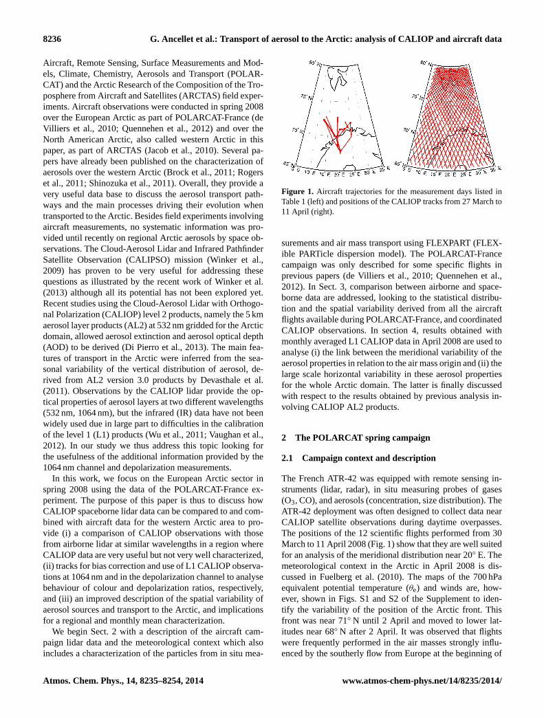
Figure 1. Aircraft trajectories for the measurement days listed inTable1 (left) and positions of the CALIOP tracks from 27 March to11 April (right).

surements and air mass transport using FLEXPART (FLEX-ible PARTicle dispersion model). The POLARCAT-Francecampaign was only described for some specific flights inprevious papers (de Villiers et al., 2010; Quennehen et al.,2012). In Sect.3, comparison between airborne and space-borne data are addressed, looking to the statistical distribu-tion and the spatial variability derived from all the aircraftflights available during POLARCAT-France, and coordinatedCALIOP observations. In section4, results obtained withmonthly averaged L1 CALIOP data in April 2008 are used toanalyse (i) the link between the meridional variability of theaerosol properties in relation to the air mass origin and (ii) thelarge scale horizontal variability in these aerosol propertiesfor the whole Arctic domain. The latter is finally discussedwith respect to the results obtained by previous analysis in-volving CALIOP AL2 products.

2 The POLARCAT spring campaign

2.1 Campaign context and description

The French ATR-42 was equipped with remote sensing in-struments (lidar, radar), in situ measuring probes of gases(O3, CO), and aerosols (concentration, size distribution). TheATR-42 deployment was often designed to collect data nearCALIOP satellite observations during daytime overpasses.The positions of the 12 scientific flights performed from 30March to 11 April 2008 (Fig.1) show that they are well suitedfor an analysis of the meridional distribution near 20◦ E. Themeteorological context in the Arctic in April 2008 is dis-cussed inFuelberg et al.(2010). The maps of the 700 hPaequivalent potential temperature (θe) and winds are, how-ever, shown in Figs. S1 and S2 of the Supplement to iden-tify the variability of the position of the Arctic front. Thisfront was near 71◦ N until 2 April and moved to lower lat-itudes near 68◦ N after 2 April. It was observed that flightswere frequently performed in the air masses strongly influ-enced by the southerly flow from Europe at the beginning of

Atmos. Chem. Phys., 14, 8235–8254, 2014 www.atmos-chem-phys.net/14/8235/2014/

G. Ancellet et al.: Transport of aerosol to the Arctic: analysis of CALIOP and aircraft data 8237

the campaign, while large section of the flights were repre-sentative of the Arctic pristine air at the end of the campaign.After 9 April, the European Arctic at latitude above 70◦ Nbecame strongly influenced by advection of biomass burningplumes advected from Asia (Quennehen et al., 2012).

The vertical structure of the aircraft flight plans were al-ways chosen to have several in situ and airborne lidar mea-surements in similar air masses in order to study the represen-tativeness of lidar products such as the attenuated backscat-ter, the colour ratio and the depolarization ratio.

During the aircraft campaign, the CALIOP spaceborne in-strument provided 80 satellite overpasses for the period 27March to 11 April in the area: 65–80◦ N, 5–35◦ E (Fig.1). Forthe area south of 72.5◦ N which corresponds to the aircraftdeployment, there are 45 CALIOP tracks leading to 433 ver-tical profiles with 80 km horizontal resolution. In this workdifferent temporal or spatial averaging will be used to analysethe CALIOP data either in the aircraft domain for compari-son with the airborne data (Sect.3) or for the whole EuropeanArctic area for all days in April 2008 (Sect.4).

2.2 Aircraft data

2.2.1 Airborne lidar measurements

During the POLARCAT campaign, the airborne lidar Le-andre Nouvelle Generation, provided measurements in itsbackscatter configuration (hereafter simplified as B-LNG)of total attenuated backscatter vertical profiles at threewavelengths: 355, 532 and 1064 nm. An additional chan-nel recorded the perpendicular attenuated backscatter verticalprofile at 355 nm. The B-LNG lidar is already described indeVilliers et al. (2010) (ADV2010) where a single flight on 11April 2008 was analysed. The methodology to calibrate theattenuated backscatter is also fully described in ADV2010 soit is only briefly described here.

In this paper, aerosol layers are identified for the 12 flightsusing 20 s averages of lidar profiles (i.e. a 1.5 to 2 km hor-izontal resolution). Only downward-pointing lidar observa-tions have been included in this work. The B-LNG data arefirst corrected for energy variations. Calibration factors arethen determined for each wavelength and for each flight bysearching for areas with very low aerosol content and by as-suming that the Rayleigh contribution controls the lidar sig-nal. These areas are chosen, as far as possible, in the up-per altitude range close to the aircraft where bias due to theaerosol transmission does not play a significant role. Theconsistency of the calibration factor is checked using differ-ent aerosol free areas and several flights, whenever possible.This is the major source of error in the calculation ofR(z),and the uncertainty (error and bias, but mostly due to bias)was found to be less than 15 % at 532 nm and less than 30 %at 1064 nm. These numbers were derived from a sensitivitystudy using different possible calibration factors and differ-ent flights. The two 355 nm channels are calibrated indepen-

Table 1.Time and positions of the B-LNG lidar vertical cross sec-tions during the POLARCAT spring campaign.

Flight Date Start Time End time Start Endlatitude latitude

24 2008/03/30 13:40 UT 14:15 UT 72.2 71.225 2008/03/31 11:30 UT 12:00 UT 71 72.326 2008/04/01 10:50 UT 11:15 UT 71.2 72.327 2008/04/03 08:15 UT 09:15 UT 68 7127 2008/04/03 08:50 UT 09:50 UT 71 6828 2008/04/06 12:30 UT 13:30 UT 69 72.729 2008/04/07 08:45 UT 09:15 UT 69.5 7129 2008/04/07 10:20 UT 11:10 UT 72 7030 2008/04/07 13:10 UT 13:45 UT 69.8 6831 2008/04/08 08:45 UT 09:45 UT 68 7131 2008/04/08 10:45 UT 11:30 UT 72 7032 2008/04/08 13:10 UT 13:45 UT 70 6833 2008/04/09 09:10 UT 09:50 UT 68 70.533 2008/04/09 11:00 UT 12:10 UT 71.5 67.834 2008/04/10 10:20 UT 11:20 UT 68 7234 2008/04/10 12:45 UT 13:15 UT 70 6835 2008/04/11 10:00 UT 11:30 UT 72.2 71.235 2008/04/11 12:30 UT 12:55 UT 69.2 68.2

dently using molecular reference and the ratio of the totalperpendicular- to the total parallel-polarized signals. How-ever, due to a reduced field of view at 355 nm, the overlapof the emitted beam with the receiver field of view limits ourability to calibrate independently the total 355 nm lidar sig-nal in the areas near the aircraft selected at the other wave-lengths. Therefore, and as CALIOP is operating at 532 nm,the measurements at 355 nm are only used for the depolar-ization ratio analysis, which is less dependent on the geo-metrical factor. The B-LNG 355 nm ratio is only a proxy forthe CALIOP one, as some differences are expected to occurdue to wavelength difference (Freudenthaler et al., 2009).

The aerosol parameters discussed in this paper and theway to calculate them are fully described in ADV2010.They are the same for airborne and spaceborne observa-tions (although depending on the wavelength for depolar-ization). They are namely (i) the attenuated backscatter ra-tios R(z) at 532 nm and 1064 nm using the CALIOP atmo-spheric density model to calculate the Rayleigh backscat-ter vertical profiles, (ii) the ratio of the total perpendicularto the total parallel plus perpendicular polarized backscat-ter coefficient (or pseudo-depolarization ratio (PDR)δ355) atthe measurement wavelength, 355 or 532 nm, respectively,(iii) the pseudo-colour ratio defined as the ratio of the to-tal backscatter coefficients at 1064 and 532 nm (PCR(z) =

R1064(z)/[16R532(z)] and (iv) the colour ratio defined asthe ratio of the aerosol backscatter coefficients at 1064 and532 nm (CRa(z) = (R1064(z) − 1)/[16(R532(z) − 1)]). Theaerosol colour ratio can be also written as CRa(z) = 2−k,wherek is an exponent depending on the aerosol microphys-ical properties (Cattrall et al., 2005).

www.atmos-chem-phys.net/14/8235/2014/ Atmos. Chem. Phys., 14, 8235–8254, 2014


Figure 2.Distribution and cumulative probability (blue) of the 532 nm (top left) and 1064 nm (top right) backscatter ratios measured by the B-LNG lidar from 30 March to 11 April. Mean, standard deviation, median and 90th percentile are given for each distribution. The distributionof the aerosol colour ratio CRa× 16 (bottom) is compared to the lines for CRa = 0.125 (k = 3), CRa = 0.25 (k = 2) and CRa = 0.5 (k = 1).

The vertical and latitudinal aircraft cross sections are listedin Table 1 and the correspondingR532 sections are shownin Fig. S3 of the Supplement. Clouds are removed from thelidar signals using a threshold both in scattering ratio anddepolarization.

This data set composed of 18 lidar meridional cross sec-tions is a representative sample of the European Arctic springaerosol distribution, as it includes different kinds of aerosolload in the lower troposphere and several cases of aerosollayers detected in the troposphere above 2 km. The probabil-ity density function (PDF) of the retrievedR(z) are shown inFig.2 to check that the lidar data processing does not produceoutliers for some flights. The homogeneity of the results be-tween the different flights has also been verified by dividingthe lidar data into three subsets: one corresponding to the be-ginning of the campaign (before 7 April), the second one tothe end (after 7 April) and the third to the overall campaign(see Table1). The differences between the three subsets aresmall when looking at the means and standard deviations ofthe distributions meaning that the error related to the cali-bration procedure is independent of the selected flight (notshown). In Fig.2, theR532(z) values do not exceed 2 (90thpercentile= 1.45) with a mean value of 1.2, as expected forthe Arctic troposphere where there are a lot of air masseswith low aerosol load (Rodríguez et al., 2012). Both the IRand the green distribution show a high left tail in the his-togram. Although most of the aerosol scattering ratios arefound near the median values (R532 = 1.15 andR1064= 1.9),

the high left tail shows that air masses withR532 > 1.4 andR1064> 2.8 are also frequently found (probability> 75 %).The uncertainty of the mean valuesR532 andR1064 can beevaluated assuming 100 independent samples for the 18 crosssections shown in Fig. S3 of the Supplement, (i.e. threevertical layers and two horizontal layers) and errors of 0.1and 0.5 forR532 andR1064, respectively, in a single layer.The distribution of the aerosol colour ratio shows a meanCRa near 0.31± 0.12, corresponding to a rather large wave-length dependence and thus to small particle size (k = 2). Asmall mode is seen to occur near 0.5 corresponding to muchsmaller wavelength dependence (k = 1) and thus to largerparticles. We also obtain a value of 0.33±0.04 for the colour

ratio CR∗a =

R1064−116(R532−1)

calculated using the mean values of

R(z) (Fig.2). Larger values near 0.5 are explained by the factthat at least 20 % of the 532 nm observations with moderateR532 values near 1.2 contribute to the tail of theR1064 distri-bution with values more than 2.4. The CRa values from theB-LNG are smaller than the range 0.4–1 (dust excepted) de-rived from the Aerosol Robotic Network (AERONET) usingsun photometers at 26 sites across the globe (Cattrall et al.,2005). However, similar values have been reported for polarair masses using lidar measurements in Alaska and Canada(Burton et al., 2012) and for a smoke layer over Ny-Alesund(Stock et al., 2011).

Since the backscatter ratio distributions points toward asignificant contribution of aerosol particles with small sizes



Figure 3. Left – comparison of B-LNG lidar attenuated backscatter averaged 120 to 200 m below the aircraft in 2.5× 10−5 km−1 sr−1 within situ measurements of CO (red) in ppbv and condensation particle counter (CPC) aerosol concentration (black) in cm−3 for the flight 35.The green curve is the aircraft altitude in 5 m unit. Right – B-LNG lidar colour ratios (PCR and CRa) in % for 10 aerosol layers where in situand lidar data can be compared (see Table2) versus the scanning mobility particle sizer (SMPS) aerosol mean diameter.

Table 2.Comparison of mean aerosol layer pseudo-(PCR) and aerosol (CRa) colour ratio measured by the B-LNG lidar and in situ measure-ments: CO mixing ratio, GRIMM integral and CPC concentrations and the mean aerosol diameter Dmeanfrom the SMPS+GRIMM spectrum.Layers data in italic or bold are respectively for low or high value colour ratios.

Date Time (UT) lat., dg alt. CO PCR B-LNG CRa B-LNG CPC GRIMM Dmeankm ppbv cm−3 cm−3 µm

30/03/08 13:45 72.0◦ N 2.2 166 17.5± 1.5 % 38± 6 % 500 300 0.2207/04/08 09:05 70.3◦ N 4.5 153 8.7± 2 % 39± 64 % 450 50 0.0708/04/08 11:20 70.7◦ N 5.0 140 14.5± 2.3 % 62± 44 % 330 25 0.1308/04/08 13:12 69.9◦ N 1.0 153 10.0± 1.5 % 19± 6 % 800 25 0.0708/04/08 13:17 69.7◦ N 4.5 200 14.7± 1.6 % 27± 6 % 800 70 0.1608/04/08 13:50 68.4◦ N 4.0 220 17.0± 1.5 % 28± 4 % 1000 150 0.1809/04/08 11:30 69.9◦ N 4.5 210 10.0± 1.8 % 26± 16 % 2500 74 0.0707/04/08 10:15 69.0◦ N 4.0 210 11.0± 1.4 % 19± 5 % 1000 50 0.1207/04/08 10:35 69.6◦ N 3.5 230 18.7± 1.5 % 31± 4 % 900 300 0.2207/04/08 11:05 71.6◦ N 3.5 200 17.0± 1.6 % 42± 6 % 700 250 0.18

(Fig. 2), we thus looked at in situ measurements where com-parisons are possible.

2.2.2 Comparison of airborne lidar with in situmeasurements

Aerosol and carbon monoxide (CO) in situ measurementsavailable on the ATR-42 aircraft are described inQuennehenet al.(2012) and ADV2010. For the aerosols, a condensationparticle counter (CPC-3010) measured the number of submi-cronic particles, while the aerosol concentrations in differentsize bins were measured by a Passive Cavity Aerosol Spec-trometer Probe (PCASP SPP-200), a GRIMM (model 1.108),and a scanning mobility particle sizer (SMPS) with a lowertime resolution (150 s). In this paper we have used the SMPS

and the GRIMM data to compute the aerosol mean geomet-rical diameter with the 150 s time resolution. Comparisonsof the CPC concentrations with the integrated concentrationsof the eight size bins of the GRIMM between 0.3 and 3 µm,provide estimates of the relative fractions of coarse aerosol.

For flights with frequent vertical motion of the aircraft, it iseasy to verify the comparability of lidar and in situ data. Sucha comparison involves looking at in situ measurements onlyduring aircraft ascents or descents crossing aerosol layersthat the lidar detects later or earlier, respectively. An exam-ple of a comparison of the lidar attenuated backscatter mea-sured 150 m below the aircraft with CO and the CPC con-centrations is shown in Fig.3 for the last flight on 11 April2008, where rather large aerosol scattering ratios were mea-sured (see Fig. S3 of the Supplement). No delay correction



is performed for this figure to compensate for aircraft speedand lidar measurement distance (this is not detectable at thisscale), but a high correlation (0.55 with significance betterthan 99 %) is nevertheless observed between lidar backscat-ter ratio and aerosol particle concentration.

Ten independent aerosol layers seen at nearly the sametime by the lidar and the other instruments on board can beused for a meaningful comparison of the lidar parameters(colour and depolarization ratios) with the aerosol concen-tration and size spectrum (Table2). The CO mixing ratiosare well correlated with the CPC data implying that combus-tion aerosols were often encountered with the largest concen-trations at the end of the campaign. Changes in the pseudo-colour ratio PCR measured by the airborne lidar correspondquite well to the variations in the aerosol mean diameter be-causeR532 variations are small enough for these 10 layersto ensure a weak dependency with the aerosol concentration(Fig. 3). The increase of CRa from 0.2 to 0.35 is also in goodagreement with the variation in the aerosol mean geometri-cal diameter if we exclude the cases with the largest erroron CRa. The uncertainty in the colour ratios are calculatedassuming a 30 and 15 % relative uncertainty for the IR andgreen scattering ratio, respectively. According to Table2, thelargest colour ratios also correspond to the largest integratedGRIMM concentrations which are high for layers with coarseaerosol. The PCR and CRa values calculated by the airbornelidar can be then considered as valuable proxies for evaluat-ing the contribution of the coarse aerosol fraction, and to firstorder (not considering speciation and size) the lidar backscat-ter ratio is a good indicator of aerosol content.

2.3 Characterization of air mass transport

The origin of the air masses sampled during the aircraftcampaign by the B-LNG lidar and by CALIOP was stud-ied using the FLEXPART model version 8.23 (Stohl et al.,2002) driven by 6-hourly European Centre for Medium-Range Weather Forecasts (ECMWF) analyses (T213L91) in-terleaved with operational forecasts every 3 h. At a given lo-cation, the model was run to perform domain filling calcu-lations in 13 boxes from 1 to 7.5 km altitude with a hori-zontal dimension of 1◦ × 1◦. The transport from the differentregions are considered for two altitude ranges:< 3 km andbetween 3 and 7 km in order to distinguish the two majortransport pathways to the Arctic: low-level flow over coldsurfaces and upper level advection by an uplifting along thetilted isentropes (Fuelberg et al., 2010; Stohl et al., 2006).This was done along the 18 aircraft cross sections and the80 CALIPSO tracks in the European Arctic domain shownin Fig. 1. For each box, 2000 particles were released over60 min and the dispersion computed for 6 days backward intime. Longer simulations lead to larger uncertainties in thesource attribution and are not considered in this work. Wehave introduced in the FLEXPART model the calculationof the fraction of particles originating below the 3 km alti-

Figure 4. Map of the regions selected to study the origin of the airmasses in the FLEXPART analysis. The red, green and blue boxescorrespond to our definition of the European, North American andEurasian regions. The two black boxes are called western and east-ern Arctic regions.

tude level for three areas with continental emissions shown inFig.4 (Europe, Eurasia, North America). We have also calcu-lated the fraction of particles present at latitudes above 70◦ Nin the troposphere above the eastern Arctic and western Arc-tic (black boxes in Fig.4). The use of the eastern Arctic frac-tion is necessary to identify the role of the Eurasian sourcesbecause with our limited simulation time (6 days), we un-derestimate the role of aged air masses related to Eurasianemissions (ADV2010).

The results first show negligible influence of the transportfrom the lower troposphere above North America and arenot considered further here. The fraction of air mass originsfor the other regions is shown for different latitude bins inFig. 5. The meridional distribution and the relative influenceof the different regions are rather similar for the CALIPSOtracks and the airborne lidar flights in the lower atmosphere.However, in the mid-troposphere, the increase of the rela-tive influence of the eastern Arctic air versus European airmasses is clearly shifted towards higher latitudes (74◦ N) forCALIOP (no contribution in the 71–72◦ N latitude band asseen for the airborne data). For both data sets, the transportof air masses from the eastern Arctic show a clear latitudi-nal increase in the lower altitude range just north of the po-lar front. For latitudes above 73◦ N, seen only by CALIOP,the overall influence of all the selected source regions ona time scale shorter than 6 days remains, however, smallerthan 40 %, implying that a large fraction of air masses hadstayed for more than 6 days in the European Arctic sectorlocated between−15◦ W and 30◦ E. Dilution, mixing anddecay of the aged mid-latitude sources are to be expected



Figure 5. Latitudinal distribution of the fraction of observations corresponding to different air mass origins calculated with FLEXPART forthe airborne lidar (left column) and CALIOP observations (right column) at altitudes< 3 km (bottom row) and between 3 and 7 km (toprow).

at these latitudes. The main differences between CALIOPand the airborne lidar sampling are (i) a significant contri-bution from Eurasian sources at low latitudes for the aircraftdata and (ii) a weaker contribution of the eastern Arctic sec-tor in the mid-troposphere for CALIOP, especially around70–72◦ N. For the airborne lidar, the Eurasian sources werenot only transported into the Arctic above the Pacific westerncoast but also by a low-level southerly flow over eastern Eu-rope from 6 to 9 April 2008. These differences are most prob-ably due to the much larger longitude band selected for theanalysis of the CALIOP data set (5 to 35◦ W) Despite thesedifferences, the overall similarity of the transport regime forboth data sets is a good indication that the small number ofaircraft flights is fairly representative of the influence of thedifferent source regions, and the data gathered may be usedto compare retrieved aerosol properties in the campaign area.

3 Analysis of CALIOP data during the aircraftcampaign

3.1 Methodology of the CALIOP data processing

A detailed description of the CALIOP operational processingcan be found in a series of papers (Vaughan et al., 2009; Liuet al., 2009; Omar et al., 2009; Powell et al., 2009). Uncer-

tainties in the AL2 colour ratio and the depolarization ratioare often very large and they are mainly used for a qualitativeanalysis of the aerosol composition and evolution (seeOmaret al.(2009) for interpretation of the colour ratio and the de-polarization ratio for aerosol classification). Most of the er-ror in the colour ratio finds its origin in the signal calibration.More recently, analyses have been conducted to improve thecalibration in version 4.0 (Vaughan et al., 2012), which con-firmed a bias in the 1064 nm channel and to a small extentthe one in the 532 nm daytime channel. We thus considereda comparison between airborne and spaceborne CALIOP L1observations as a first step.

In ADV2010, the AL2 CALIOP products were analysedfor one particular flight of the POLARCAT campaign us-ing layers detected at 80 km horizontal resolution and witha 3 % threshold value for the layer optical depth at 532 nm.Comparisons between the CALIOP AL2 and airborne lidarPCR then showed larger values for CALIOP in the aerosollayers of the 11 April flight. Considering the large uncer-tainty in the weak aerosol layers detected in the AL2 productover the Arctic, averaging of the L1 version 3.01 CALIOPdata is used in this paper to analyse the 45 CALIPSO tracksavailable in the aircraft campaign domain. The comparisonof the aerosol parameter PDF obtained for the campaign pe-riod and the campaign area is considered as more appropriate



to validate the satellite aerosol data than relying on optimizedcollocations of aircraft and satellite data, which would givea very small number of cases. Gridded latitudinal distribu-tions with a 1.25◦ resolution in the campaign area are used tocheck the coherency of the two data sets.

The CALIOP L1 attenuated backscatter coefficientsβ1064andβ532 are available with 333 m horizontal resolution up tothe 8.2 km vertical level and with 1 km resolution at higheraltitude. Before making any horizontal or vertical averagingof these data, it is necessary to apply a cloud mask on the L1data set. This cloud mask is based on the cloud mask featuresavailable in the level 2 version 3.01 CALIOP cloud (CL2)data products for the 5 km horizontal resolution. Additionalchecks have, however, been added to verify that cloud lay-ers are not misclassified. First, ice cloud layers, detected inthe 80 km horizontal resolution profile, must have a pseudo-colour ratio> 0.6 and a layer depolarization ratio> 0.3. Ifthis is not the case, the three brightness temperatures,T12µm,T10µm and T8µm, measured by the IR imaging radiometer(IIR) installed on the same platform (Garnier et al., 2012)are used as an additional test to classify the layer as a cloudlayer or as an aerosol layer. Based on simulations, the crite-rion to keep a layer as a cloud layer is that the differencesT8µm–T12µm andT10µm–T12µm must be positive (Dubuissonet al., 2008). Second, if the cloud layer is also detected inthe 333 m resolution CL2 data products, it is always kept asa cloud as explained inLiu et al. (2009). Only very denseaerosol layers (scattering ratio> 3) are misclassified whenadding these two conditions.

Theβ1064 andβ532 data are then removed below the high-est cloud top altitude for each vertical profile, when the op-tical depth (OD) of the cloud is larger than 1. For semi-transparent clouds with smaller ODs (< 0.9), a transmissioncorrection is performed. The data are also excluded in the100 m layer just above the cloud top to avoid any error inthe cloud top estimate. The cloud filtering is then very con-servative in order to exclude a possible bias in the aerosolparameters measured below clouds when the spectral varia-tion of the overlaying cloud attenuation has to be taken intoaccount.

The cloud-filtered 333 m attenuated backscatter verticalprofiles are then over 80 km and vertically over 150 m with alow pass second-order polynomial filter second-order poly-nomial filter to improve the signal-to-noise ratio. The 80 kmmean attenuated backscatter ratioR532(z) andR1064(z), themean aerosol colour ratio and the mean 532 nm volume de-polarization ratio are finally calculated using the moleculardensity and ozone vertical profiles available at 33 standardaltitudes in the CALIOP data products.

As explained before, two different methods are used forcomparison with airborne lidar observations:

– PDF of aerosol parameters using all the 80 km, 150 maveraged profiles available in the aircraft campaign area,i.e. with 0< z < 7 km, latitude between 65 and 72.5◦ N,

longitude between 5 and 35◦ E, from 27 March to 11April 2008

– a latitudinal cross section in the same campaign areawhere 80 km, 150 m averaged profiles are gridded into5× 14 boxes with a 1.25◦ latitude and 500 m verticalresolution.

3.2 Impact of the 1064 nm CALIOP calibration on theaerosol colour ratio

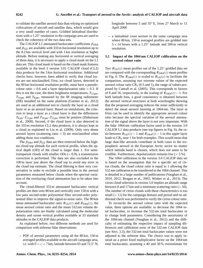
Two R532(z) mean profiles out of the 1.25◦ gridded data setare compared with the correspondingR1064(z) mean profilesin Fig. 6. TheR1064(z) is scaled toR532(z) to facilitate thecomparison, assuming two extreme values of the expectedaerosol colour ratio CRa (0.5 and 1), the range of values pro-posed byCattrall et al.(2005). This corresponds to factorsof 8 and 16, respectively, in the scaling ofR1064(z) − 1. Forboth latitude bins, a good consistency is obtained betweenthe aerosol vertical structures at both wavelengths showingthat the proposed averaging reduces the noise sufficiently todetect the mean aerosol layering at 1064 nm. The layer at8 km can be used to identify the appropriate aerosol colourratio because the spectral variation of the aerosol attenua-tion of the signal above the layer is not very important. Withthe lidar 1064 nm calibration factor used in the version 3.0CALIOP L1 data products (see top figures in Fig.6), the ra-tio betweenR532(z) − 1 andR1064(z) − 1 in this upper layerleads to CRa near 1 for both examples. This would mean thatlarge dust-like aerosols contribute in both cases to the tro-pospheric aerosol in the European Arctic sector no matterwhich latitude band is chosen, which does not seem to becredible. Furthermore, depolarization remains low (< 5 %).

The 1064 calibration in the version 3.0 CALIOP data setis based on the assumption that for a specific set of cir-rus clouds, the cloud colour ratio is equal to 1 allowing the532 nm calibration to be transferred to the 1064 channel. Thisis detailed in a large number of publications (Vaughan et al.,2010, 2012; Reagan et al., 2002; Winker et al., 2013). Thecirrus cloud selection in version 3.0 implies an altitude rangebetween 8 and 17 km and a minimum scattering ratio (> 50).The number of cirrus clouds with these characteristics is toosmall (< 11) for the campaign domain and period and no ad-ditional check was performed to verify the cirrus colour ratio.

To reconcile the aerosol colour ratio with the expectedvalue, three options are available: to decrease the 1064 to-tal backscatter, to increase the 532 nm total backscatter orto change both parameters. Considering the uncertainty ofthe 1064 nm channel (Vaughan et al., 2012) and the diffi-culty of estimating the respective impact of sampling dif-ferences and calibration error of the 532 nm CALIOP data(see Sect.3.3), the 532 nm total backscatter values were notadjusted to the airborne data. The choice was to apply in-stead an a priori fixed multiplicative factor on the 1064 nmtotal backscatter, assuming a 40 and 30 % overestimate for



Figure 6. Mean attenuated backscatter ratio for the 532 nm (green) and 1064 nm filtered level 1 CALIOP (blue and red). The 1064 nm valuesare scaled to the 532 nm values using expected lowest CRa = 0.5 (red) and largest CRa = 1 (blue). The top and bottom row respectively arefor uncorrected and calibration corrected IR data.

daytime and night-time conditions, respectively. For daytimethis is estimated from the B-LNG mean scattering ratios (seeFig. 2). A reduced value was considered for night-time, aslinked to the ratio in the daytime and night-time scale fac-tors in version 3.0 CALIOP data as mentioned in previousanalyses (Wu et al., 2011; Vaughan et al., 2012). The ratiobetweenR532(z)−1 andR1064(z)−1 then becomes more re-alistic since it leads to CRa intermediate between 0.5 and 1for the upper layer near 8 km, and also for the layers in thelower troposphere.

To verify that large CRa for uncorrected IR data is not re-lated to a bias introduced by the averaging of many profilesbefore the calculation of the colour ratio, we have looked attheR532(z) versusR1064(z) scatter plot using all the 80 kmresolution CALIOP-filtered data for the altitude ranges, 0–7 and 13–15 km. The scatter plots are presented in Fig.7for the uncorrected and corrected IR data using a frequencycontour plot. Since we expect a very weak aerosol con-tribution in the 13–15 km altitude range, no specific cor-relation are found betweenR532(z) versusR1064(z). Thenoise of the 532 nm attenuated backscatter is of the order of0.15× molecular backscatter while the noise of the 1064 nmattenuated backscatter is 3 and 4× molecular backscatterwith and without the correction of IR data, respectively. Ac-counting for the factor of 16 between the two molecular con-

tributions, the noise in the IR channel is only 1.2 times largerthan the 532 nm noise value when correcting the IR data.Such a ratio is comparable to the analysis ofWu et al.(2011)at 16 km for all the daytime CALIOP data. No correctionof the IR would mean a ratio of 1.7 between the 532 and1064 nm signal noise level. The overestimate of the 1064 nmbackscatter is even more likely when looking at the scatterplot for the altitude range 0–7 km. The slope of the regressionline is indeed too small for the uncorrected IR data since itcorresponds to many CRa values larger than 1. The frequencyof clean air masses (R = 1) is also more consistent betweenthe 532 nm and the 1064 nm observations after the correctionof the IR overestimation provided that the 532 nm scatteringratio is correct.

The impact on the cirrus colour ratio was not evaluated forthe small number of occurrences in our domain but it wouldimply a positive bias of 40 % when using the version 3.0 cal-ibration. Such a bias is larger that the uncertainty of±20–30 % proposed for the 1064 nm calibration procedure (Wuet al., 2011; Vaughan et al., 2012). We must recall, however,that a 40 % bias can be also accounted for if we assume anegative bias of 5 % for the 532 nm scattering ratio. As ex-plained in Sect.3.3, this hypothesis was not considered inthis work and the recalibration of the 1064 nm signal waschosen. It will be interesting to test this hypothesis using the



Figure 7. Correlation between the 532 and 1064 nm filtered level 1 CALIOP backscatter ratio from 27 March to 11 April 2008, at altitudesfrom 0 to 7 km (top row) and 13 to 15 km (bottom row) using either uncorrected (left) or corrected (right) IR backscatter data. Regressionline is the dashed-dotted blue line. The linesk = −1, 0, 1 are for tropospheric aerosol distributions with CRa = 2, 1, 0.5m, respectively.

new version 4 level 1 CALIOP data which will be available.In the new version 4.0, the cirrus cloud selection for the 1064calibration (i.e. with a cloud colour ratio of 1) has been up-dated (cloud temperature instead of altitude selection, use ofthe cloud depolarization ratio) providing more cirrus cloudsand better altitude selection for the Arctic (Vaughan et al.,2012).

3.3 Comparison of airborne lidar and CALIOP

3.3.1 Analysis of the statistical distribution

Using the data set averaged over the campaign pe-riod/domain, the distributions of the CALIOP correctedR1064andR532 are shown in Fig.8 for the range 0–7 km and13–15 km. The latter corresponds to very low aerosol con-centrations. It has a mean and a median with a difference lessthan 0.02 at 532 nm and 0.3 at 1064 nm from the expectedscattering ratio of 1. The large standard deviations of 0.3 at532 nm and 4 at 1064 nm are expected at this altitude levelwhere the molecular backscatter decreases significantly.

The R1064 mean (2.3) is close to the airborne lidar value(2.1) considering an error of the mean of the order of 0.1and even though the standard deviation of the noisy CALIOP

R1064 distribution is 1.7 times larger than the airborne lidarcorresponding value. The same ratio is observed between theairborne and CALIOPR532 standard deviation. Therefore,this confirms the validity of the estimated correction factoralthough with a large statistical error (about 30 % on the co-efficients) for the 1064 nm CALIOP profiles selected in ourstudy of the Arctic region.

Contrary to the airborne lidar distribution, the CALIOPR532 distribution in the troposphere below 7 km does notshow many layers with elevated aerosol concentrations asshown by a lower value of the 90th percentile (1.34 forCALIOP instead of 1.45 for the airborne lidar). The largerstandard deviation (0.34 instead of 0.2) is related to thepoorer signal-to-noise ratio of the satellite data set. The lowervalue for the 532 nm mean (1.13 instead of 1.21) is largerthan the expected uncertainty of the mean of the CALIOPdistribution which is of the order of 0.01. This uncertainty ofthe mean is calculated assuming an error of 0.4 for a singleCALIOP measurement (i.e. the width of the distribution forthe negative values) and assuming 1700 independent layersout of 28 872 data points available in the 0 and 7 km altituderange above the campaign domain (i.e. considering a 1 kmvertical sampling instead of the 60 m vertical resolution toensure independence). Since we compare patchy data, it is



Figure 8. Distribution of the 532 nm (top left) and 1064 nm (top right) filtered level 1 CALIOP backscatter ratios at altitudes from 0 to 7 km(green) and 13 to 15 km (red) from 27 March to 11 April in the aircraft flight area. Mean, standard deviation, median and 90th percentile aregiven for each distribution. The distribution of the aerosol colour ratio 16× CRa (bottom) is compared to the lines for CRa = 0.125 (k = 3),CRa = 0.25 (k = 2) and CRa = 0.5 (k = 1).

also important to assess how the averaging of aerosol lay-ers with observed clear air scenes may explain this differ-ence. For example, the difference between the airborne andCALIOP R532 averages can be explained if there are twiceas many layers with low aerosol load (R532 < 1.05) in theCALIOP data set. This may be related to the fact that in ourCALIOP data processing we remove all the total backscattervalues below clouds. It is also necessary to check whetherthis difference may also be due to (1) an overestimate of the532 nm CALIOP calibration factor (2) an underestimate ofthe airborne lidar calibration factor. Positive differences dueto 532 nm daytime calibration uncertainty were also obtainedby Rogers et al.(2011) when comparing NASA High Spec-tral Resolution Lidar (HSRL) and CALIOP data for measure-ments at high latitudes in the Northern Hemisphere, but themean difference is not higher than 3 %. The remaining 5 %uncertainty of the mean difference can be accounted for bya systematic error in the airborne lidar calibration when as-suming no aerosol in the altitude range which corresponds tothe smallest attenuated backscatter coefficient. Comparisonswith other observations confirmed that 532 nm CALIOP datacould be underestimated by about 5 %, due to the occurrenceof residual stratospheric aerosols at the normalization alti-tude (Vernier et al., 2009). This would be supported by the

fact that we obtain a very small value (< 2 %) of the 532 nmmean aerosol scattering ratio in the 13–15 km range whenusing the version 3.0 calibration.

The averageCRa is 0.44± 0.8 for CALIOP which is notvery far from the airborne lidar value (0.31± 0.12) consid-ering the factor of 6 between the two standard deviations ofthis parameter (Fig.8). For the noisy satellite data, a betterproxy isCRa

∗= 0.65± 0.1, i.e. the mean colour ratio calcu-

lated with (R532− 1) and (R1064− 1), which is then 2 timeslarger than the similar ratio for the airborne lidar. This canbe explained by the 10 % bias inR532 which is always lessthan 1.35. Therefore, this difference cannot be interpreted asa stronger contribution of the coarse aerosol fraction in thesatellite observations. Despite this bias in the order of mag-nitude ofCR∗

a, it is important to verify if the relative spatialor temporal variability is detected by the satellite data.

3.3.2 Analysis of the latitudinal distribution

The latitudinal variability of the aerosol properties is stud-ied using the CALIOP latitudinal grid data set described ear-lier, i.e. considering 5 successive 1.25◦ latitude bins and 14vertical layers of 500 m. The airborne lidar data are analysedonly for layers where the aerosol content is high enough to be



Figure 9. Latitudinal distribution of 532 nm backscatter ratio (left), aerosol colour ratio (middle) and pseudo-depolarization ratio (right) forthe airborne lidar observations (top) and filtered level 1 CALIOP (bottom) at altitudes< 3 km during the aircraft campaign. The colours arefor different air mass origins estimated with FLEXPART (see text).

observed in the 1064 nm profiles. There are 90 well definedand independent aerosol layers identified in the 18 lidar crosssections at latitudes less than 72.5◦ N. For the campaign pe-riod, we do not have many data below 1 km (see Fig. S3 in theSupplement), so the comparison of the latitudinal variationsis made for the two following altitude ranges: 1–3 and 3–7 km. The latitudinal distributions ofR532, CRa andδ532 (orδ355) are shown for both data sets in Figs.9 and10. For eachaerosol layer, the FLEXPART analysis was used to distin-guish between European or Eurasian air masses transportedby the southerly flow on one hand, and the Eurasian or NorthAmerican sources advected in our domain through the polardome on the other hand. The green and red data points cor-respond to eastern and western Arctic origins, respectively,while the black points, labelled South in Figs.9 and10, in-dicate the influence of mid latitude sources directly advectedby the southerly flow. Each point in the airborne lidar plotscorresponds to a single layer observed by the aircraft, whilefor CALIOP it corresponds to an average of several layers atthe same altitude in the selected latitude band.

Lower troposphere (< 3 km)

For the lower troposphere (Fig.9), the airborne lidar does notshow a clear latitudinal dependency of the aerosol scatteringratios for the eastern Arctic and European/Eurasian sources.

A decrease of the occurrence of elevated aerosol concentra-tions is, however, observed by CALIOP at the lowest lati-tudes. This is especially true for the eastern Arctic aerosoltype. The increase of cloudiness at southern latitudes may ex-plain this evolution because of the lower probability of obser-vations in the lowermost troposphere. The significant numberof CALIOP R532 values below 1.1 identified in the statisti-cal analysis discussed in the previous section is seen at alllatitudes. Although the range of CRa are larger for CALIOP(0.6–1.1 instead of 0.2–0.5 for the airborne lidar), the relativelatitudinal variations are somewhat similar with a maximumbetween 70 and 72◦ N, especially when focusing on the east-ern Arctic air masses.

The δ355 values measured by the airborne lidar are lessthan 1.5 % for no depolarization and exceed 2 % when depo-larization is present, while the uncertainty is of the order of0.2 %. Values ofδ532 measured by CALIOP are larger, rang-ing from 3 to 11 %, because of a spectral variation of theaerosol depolarization ratio. Assuming a backscatter ratio ofthe order of 1.1 at 355 nm and 1.3 at 532 nm, such a changeof PDR corresponds to a change of the aerosol depolarizationratio from 5 % at 355 nm to 10 % at 532 nm. Such a spectralvariation was observed byGross et al.(2012) in a mixture ofvolcanic ash and marine aerosol when hygroscopic aerosolwas present but at a size small enough to decrease only the355 nm parallel backscatter. A similar kind of mixture could



Figure 10.Latitudinal distribution of 532 nm backscatter ratio (left), aerosol colour ratio (middle) and pseudo-depolarization ratio (right) forthe airborne lidar observations (top) and filtered level 1 CALIOP (bottom) at altitudes between 3 and 7 km during the aircraft campaign. Thecolours are for different air mass origins estimated with FLEXPART (see text).

exist in our European Arctic domain and was found in air-craft measurements over Alaska in April 2008 (Brock et al.,2011). Regarding the latitudinal increase of the depolariza-tion ratio, it was observed for both data sets.

Mid-troposphere (> 3 km)

For the mid-troposphere (Fig.10), the latitudinal decreaseof the backscatter ratio is observed in the airborne and theCALIOP lidar data, especially for the southerly flow. TheCALIOP observations are never strongly related to the east-ern Arctic at latitudes less than 75◦ N for altitudes above3 km as discussed in Sect.2.3. Thus, the comparison is onlymeaningful when considering the air masses advected by thesoutherly flow. For both data set, the latitudinal variations areconsistent: a small increase of CRa, a decrease of the pseudo-depolarization ratio.

To conclude, there are significant differences in the mag-nitude of CRa (mainly related to differences in the magni-tude ofR532) and in the magnitude of the depolarization ra-tio (related to the expected spectral variation between 532and 355 nm), but the spatial variations are rather similarfor both data sets considering the limited coverage of theairborne data. The comparison of theR532 1.25◦ averagedvertical profiles is also useful to discuss the relative influ-ence of calibration error and sampling differences between

CALIOP and the B-LNG airborne lidar (Fig.11). For the al-titude ranges with the largest aerosol content (below 2 kmand above 4 km), the order of magnitude ofR532 is similarand varies in the same direction when increasing the latitudebin. The largest differences are in the 1.5 to 4 km altituderange corresponding to the lowest values ofR532 where theCALIOP data are frequently below 1.1. Therefore, the biasin R532 is not only related to calibration issues, but also tothe fact that the airborne lidar saw more air masses with sig-nificant aerosol content in the altitude range of 1.5 to 4 km.This may be related to the specific targeting of the aircraftflights to sample such layers and also to the fact that manyof these layers are observed below 4 km in the frontal zonewhere overlying clouds (see Supplement) make the detectionby the CALIOP overpasses more difficult. The wider longi-tude range chosen for the CALIOP data set do not compen-sate for this difference in the observed air masses. Since thedifference in the magnitude of the 532 nm backscatter ratio isnot only related to a calibration uncertainty in one instrumentor both, but also to differences in the number of observationswith low aerosol content in the altitude range 1.5 to 4 km, wechoose not to apply any correction to the 532 nm CALIOPdata set.



Figure 11.B-LNG lidar (left) and CALIOP (right) vertical profiles of the 532 nm backscatter averaged over a 1.25◦ latitude band and for theaircraft period.

4 CALIOP characterization of the aerosol layerproperties in April 2008

4.1 Latitudinal variability in the European Arctic

In this section, the CALIOP data are now analysed for 30days in April 2008 to improve further the signal-to-noise ra-tio. The latitudinal distribution of aerosol properties in theEuropean Arctic is still derived using average CALIOP ver-tical profiles for 1.25◦ latitude bins, but over a larger domainbetween 65 and 80◦ N. Two specific altitude ranges (0–2 kmand 5–7 km) have been selected because they correspond tothe largest aerosol load identified in the mean vertical profileover the European Arctic (Fig.11).

Lower troposphere (0–2 km)

In the lower troposphere, the meridional cross section ofR532 reveals that the largest aerosol scattering in the plan-etary boundary layer (PBL) is for air masses with an easternArctic origin and mainly in the Arctic frontal zone between69 and 75◦ N (Fig. 12). The large error bars correspond-ing to small aerosol loads encountered in the Arctic limitthe quantitative analysis of the CRa meridional distribution.The slight increase of CRa with latitude is mainly related tothe variation of CRa with the air mass origin. The easternArctic aerosol layers show CRa > 1 while air masses witha European origin correspond to CRa ≈ 0.7. Theδ532 crosssection shows significant depolarization (near 10 % for themonthly average) within the 70–73◦ N latitude range. Con-sidering the high scattering ratios, the significant fraction ofcoarse aerosol (CRa near 1) and depolarization, a contribu-tion of ice crystal formation in the frontal zone is very likelyin this latitude range. When excluding these specific cases,the European aerosol layers have larger depolarization thaneastern Arctic air masses. Larger and more spherical aerosolsfor the eastern Arctic layers is not so surprising considering

aerosol ageing in air masses transported from Asia (Masslinget al., 2007).

Mid-troposphere (5–7 km)

In the mid-troposphere (5–7 km), there is a general decreasein R532 with latitude for the European air masses, while itincreases for air masses with an eastern Arctic origin. So incontrast to the PBL there is a minimum of aerosol contri-bution near 72◦ N. This can be explained if one assumes asignificant wet removal of particles during upward verticaltransport within the Arctic front. As observed for the lowertroposphere, CRa values are lower for European air masses(near 0.5) than for Asian Arctic origin (near 0.8). We donot see the large depolarization values related to the possi-ble presence of ice crystals above 5 km, since they are nottransported out of the PBL. However, the meridional distri-bution of the depolarization shows a clear decrease at thehighest latitudes. The latitudinal increase of CRa associatedwith a decrease in depolarization could be explained by theincreasing importance of aged anthropogenic aerosol and notto a strong influence of dust particles. The in situ analysis ofthe size distribution made inQuennehen et al.(2012) indeedshowed that Asian anthropogenic aerosol contributed signif-icantly to the accumulation mode.

4.2 Large scale distribution in the Arctic domain

April monthly averages forR532, CRa and δ532 have beencalculated for the complete Arctic domain (latitude> 60◦ N)in horizontal boxes of 300 km× 300 km. The CRa values areonly given whenR532 > 1.25 to focus on the contribution ofsignificant aerosol plumes, and to avoid large errors in CRadue to small scattering ratios. The fraction of CALIOP obser-vations available (i.e. not below a cloud) in the selected alti-tude range is also given to estimate the number of effectiveCALIOP tracks in every box. According to Fig.1 a minimum



Figure 12.Latitudinal distribution of 532 nm backscatter ratio (left), aerosol colour ratio (middle) and pseudo-depolarization ratio (right) forfiltered level 1 CALIOP in April 2008 at altitudes< 2 km (bottom) and between 5 and 7 km (top). The origin of the layers are estimated withFLEXPART (see text).

number of 10 overpasses is needed for the data to be repre-sentative of a monthly mean. This corresponds to a fractionof 50 % at 65◦ N and 20 % at 80◦ N.

Lower troposphere (0–2 km)

In the lower troposphere (Fig.13), theR532 map shows theextent of a northern Atlantic aerosol contribution with valuesremaining larger than 1.5 above 70◦ N. Sea salt and sulfateaerosol are known to contribute to the increase of aerosolscattering over the North Atlantic in winter and early spring(Smirnov et al., 2000; Yoon et al., 2007). The CRa map indi-cates a gradual increase of CRa with latitude over the north-ern Atlantic: values< 0.7 occur near the mid-latitude sourceslocated below 65◦ N but CRa > 0.9 are frequent above 70◦ N.The latitudinal gradient of CRa over the northern Atlanticcan be related to the growing influence of a different kindof aerosol, since the probability of aerosol particle trans-port from the eastern Arctic is increasing as discussed inthe previous section. Aerosol composition analysis on boardthe NOAA ship during the International Chemistry Exper-iment in the Arctic Lower Troposphere (ICEALOT) cam-paign (Frossard et al., 2011) has shown that marine and sul-fate aerosol represent 70 % of the submicronic aerosol com-position in the northern Atlantic east of Iceland and they also

found that the sulfate contribution increases with latitude.This is broadly consistent with the CALIOP observations.

A local maximum in theR532 map is also observed overSiberia between 90 and 110◦ E with a latitudinal extent upto 70◦ N in the Taymyr peninsula. In spring 2008, this areawas known to have been influenced on one hand by local an-thropogenic emissions from gas flaring (Stohl et al., 2013),and on the other hand by early spring forest fires in Russia(Warneke et al., 2010). The maximum in northern Siberiais also seen for the same area in the AOD analysis made byWinker et al.(2013) using CALIOP data for the winter periodbefore the fire period, implying a significant contribution ofanthropogenic emissions. The CRa values< 0.7 are similarto those observed below 65◦ N over the Atlantic Ocean. Nosignificant depolarization is observed in these two source re-gions implying very little impact from dust or volcano emis-sions in this altitude range. The difference of CRa betweenthe European Arctic and the source region in Russia impliesa growing of the aerosol particles during transport and age-ing if one assumes that most of the aerosol layers observedin European Arctic originate from Eurasia (see previous sec-tion).



Figure 13. Map of the 532 nm backscatter ratio (top left), aerosol colour ratio (top right), pseudo-depolarization ratio (bottom left) andfraction of cloudless observations (bottom right) using the April 2008 filtered level 1 CALIOP data in the 0–2 km altitude range. Colourscales are in relative units.

Mid-troposphere (5–7 km)

In the mid-troposphere (Fig.14), theR532 map gives a verydifferent picture of the link between the Arctic aerosol dis-tribution and the mid-latitude sources. There is, first, a broadaerosol maximum from eastern Siberia to western Alaska atlatitudes between 60 and 75◦ N and, second, another maxi-mum over the Hudson bay. The eastern Arctic domain northof 70◦ N is not as clean as in the lower troposphere, be-ing consistent with an efficient transport pathway from mid-latitudes along the tilted isentropic surfaces (Harrigan et al.,2011). The western Arctic and northern Atlantic are rela-tively free of aerosol particles in the mid-troposphere. Thisis somewhat contradictory with the known uplift of low-levelNorth American air pollution over western Greenland (Har-rigan et al., 2011; Ravetta et al., 2007). The contrast betweenthe large aerosol concentrations found in the northern At-lantic lower troposphere and the low values above is alsoconsistent with the conclusions of several papers (Law andStohl, 2007; Harrigan et al., 2011) about the transport path-way of European emission being most efficient in the lowertroposphere.

The global cloud distribution can be obtained from theDARDAR (raDAR/liDAR) products, which are based onCloudSat and CALIOP data according to a variationalscheme, on a 60 m vertical resolution and 1 km horizontalresolution grid (Delanoë and Hogan, 2008). The synergy be-tween lidar and radar is indeed needed to have a detailed pic-ture of the cloud vertical profile (Ceccaldi et al., 2013). It has

been used here to calculate the cloud fraction at different al-titudes during the month of April 2008 in 4 different latitudebands from 60 to 80◦ N (Fig. 15). The latitudes with largecloudiness in both the mid and upper troposphere show up-ward frontal lifting by warm conveyor belts (WCB) near theBering Strait and the western coast of Greenland. The lat-ter shows the largest cloudiness at 5 km. This may explainthe low aerosol concentration downwind of Greenland dueto efficient removal of aerosol. One can also notice the goodcorrelation between the high values of the low-level cloudfraction and the large aerosol load observed above 70◦ N inthe European Arctic.

The aerosol depolarization and colour ratio distributionsshow little depolarization (except over the Hudson bay) inthe large scale aerosol plumes seen in the mid-troposphere.However, as in the lower troposphere, the CRa increase at lat-itudes> 70◦ N is consistent with aerosol ageing when reach-ing the highest latitudes.

5 Conclusions

In this paper we have analysed aerosol airborne (B-LNG) andspaceborne (CALIOP) lidar data related to the transport ofmid-latitude sources into the Arctic. The main results are thefollowing:

– A campaign was held in April 2008 in the EuropeanArctic with 18 aircraft cross sections and 80 CALIPSOtracks over 15 days improving our ability to identify the



Figure 14. Map of the 532 nm backscatter ratio (top left), aerosol colour ratio (top right), pseudo-depolarization ratio (bottom left) andfraction of cloudless observations (bottom right) using the April 2008 filtered level 1 CALIOP data in the 5–7 km altitude range. Colourscales are in relative units.

Figure 15.Zonal vertical cross sections of the cloud fraction derived from the DARDAR products for April 2008 in 4 latitude bands from 60to 80◦ N. The longitudinal resolution is 5◦ and the vertical resolution is 60 m.

transport of aerosol layers to the Arctic, especially fromthe analysis of the satellite data.

– Analysis of the B-LNG backscatter ratioR532 andR1064at two wavelengths for the calculation of the aerosolcolour ratio (CRa) has been successfully compared within situ aerosol measurements on board the aircraft.The CRa increase corresponds to a similar increase in

the mean aerosol diameter, showing the importance ofmulti-wavelength analysis. It also emphasizes the needfor accurate lidar calibration.

– Simulations with the FLEXPART model show that thelimited number of airborne lidar cross sections are rep-resentative of the main characteristics of the air masstransport in April 2008: increase with latitude of the



aged air masses from the eastern Arctic region at alti-tudes below 3 km, large influence of the mid-latitudessources directly transported by the southerly flow at al-titudes above 3 km.

– Comparisons are performed between B-LNG andCALIOP backscatter ratioR532 andR1064 at two wave-lengths, including the calculation of the aerosol colourratio and of the depolarization ratio (PDR) at 532 and355 nm. Comparisons are based on the analysis of 15-day averages and L1 CALIOP data processing insteadof AL2 CALIOP operational products. Specific aver-aging methods can then be applied. The cloud screen-ing, needed when using L1 lidar data, is based onCL2 CALIOP data products and the IR CALIPSO ra-diometer data. A recalibration of the CALIOPR1064in the Arctic was chosen to reduce the positive bias ofthe CALIOP data with respect to airborne observationsof the colour ratio. A fixed factor was applied to the1064 nm attenuated backscatter data, of 1.3 and 1.4, re-spectively, for night-time and daytime orbits. This valuecould be significantly smaller if a small negative bias ofthe 532 nm CALIOP lidar signal is also corrected, butthis hypothesis was not applied in this work. The use ofthe new version 4.0 data which will be available verysoon would certainly help to address this question.

– Comparisons of the statistical distributions in the alti-tude range 0–7 km show no significant bias forR1064when correcting the CALIOP 1064 nm data but a−8 %difference between the CALIOP and B-LNGR532 data.The latter might be related to a calibration problem ofeither the B-LNG or the CALIOP instrument. However,being largest in a specific altitude range between 1.5 and4 km, the differences of the spatial averaging of airborneand satellite data are also to be considered. The differ-ence in the magnitude of CRa is mainly related to thisoverestimation ofR532 in the B-LNG data. The depo-larization ratio is not measured at the same wavelengthand its spectral variation follows that of hygroscopicaerosol often at a size small enough to be detected onlyat 355 nm (Gross et al., 2012).

– The latitudinal distribution of the colour ratio and thedepolarization ratio is similar for the B-LNG and theCALIOP data sets, especially considering the limitednumber of aircraft flights. It is a good indication that,despite possible bias in these two parameters when com-paring them, airborne and satellite data are still valuablefor the analysis of the aerosol growth or the relative frac-tion of dust or volcanic ashes using CALIOP observa-tions.

– The monthly average analysis of the CALIOP colourand depolarization ratio in the European Arctic areashows that larger (higher CRa) and more spherical

aerosol (low PDR) are expected in the air masses trans-ported from the eastern Arctic both in the lower tropo-sphere (0–2 km) and in the mid-troposphere (5–7 km).Less aerosol is present in the mid-troposphere near thearctic front (70–74◦ N) while significantR532 and depo-larization ratio are seen in the lower troposphere, possi-bly related to the presence of ice crystals.

– The global distribution of the CALIOP monthly anal-ysis reveal two regions with large backscatter below2 km: the northern Atlantic between Greenland andNorway, and the Taymyr peninsula. The CRa increasebetween the source regions and the observations at lat-itudes above 70◦ N implies a growth of the aerosol sizeonce transported to the Arctic. The distribution of theaerosol optical properties in the mid-troposphere is con-sistent with the transport pathways proposed inHarri-gan et al.(2011): (i) low-level advection in northern Eu-rope, (ii) isentropic uplifting of pollution and biomassburning aerosol in northern Siberia and eastern Asia and(iii) aerosol washout by the North Atlantic warm con-veyor belts.

The Supplement related to this article is available onlineat doi:10.5194/acp-14-8235-2014-supplement.

Acknowledgements.The UMS SAFIRE is acknowledged forsupporting the ATR-42 aircraft deployment and for providingthe aircraft meteorological data. The POLARCAT-France andCLIMSLIP projects were funded by ANR, CNES, CNRS/INSUand IPEV. The FLEXPART team (A. Stohl, P. Seibert, A. Frank,G. Wotawa, C. Forster, S. Eckhardt, J. Burkhart, H. Sodemann) isacknowledged for providing the FLEXPART code. NASA, CNES,the ICARE and the LARC data centre are gratefully acknowledgefor supplying the CALIPSO data.

Edited by: G. Vaughan

References

Brock, C. A., Cozic, J., Bahreini, R., Froyd, K. D., Middlebrook,A. M., McComiskey, A., Brioude, J., Cooper, O. R., Stohl, A.,Aikin, K. C., de Gouw, J. A., Fahey, D. W., Ferrare, R. A.,Gao, R.-S., Gore, W., Holloway, J. S., Hübler, G., Jefferson, A.,Lack, D. A., Lance, S., Moore, R. H., Murphy, D. M., Nenes,A., Novelli, P. C., Nowak, J. B., Ogren, J. A., Peischl, J., Pierce,R. B., Pilewskie, P., Quinn, P. K., Ryerson, T. B., Schmidt, K.S., Schwarz, J. P., Sodemann, H., Spackman, J. R., Stark, H.,Thomson, D. S., Thornberry, T., Veres, P., Watts, L. A., Warneke,C., and Wollny, A. G.: Characteristics, sources, and transport ofaerosols measured in spring 2008 during the aerosol, radiation,and cloud processes affecting Arctic Climate (ARCPAC) Project,Atmos. Chem. Phys., 11, 2423–2453, doi:10.5194/acp-11-2423-2011, 2011.


http://dx.doi.org/10.5194/acp-14-8235-2014-supplement

http://dx.doi.org/10.5194/acp-11-2423-2011



Burton, S. P., Ferrare, R. A., Hostetler, C. A., Hair, J. W., Rogers, R.R., Obland, M. D., Butler, C. F., Cook, A. L., Harper, D. B., andFroyd, K. D.: Aerosol classification using airborne High Spec-tral Resolution Lidar measurements – methodology and exam-ples, Atmos. Meas. Tech., 5, 73–98, doi:10.5194/amt-5-73-2012,2012.

Cattrall, C., Reagan, J., Thome, K., and Dubovik, O.: Variabil-ity of aerosol and spectral lidar and backscatter and extinc-tion ratios of key aerosol types derived from selected AerosolRobotic Network locations, J. Geophys. Res., 110, D10S11,doi:10.1029/2004JD005124, 2005.

Ceccaldi, M., Delanoë, J., Hogan, R. J., Pounder, N. L., Protat, A.,and Pelon, J.: From CloudSat-CALIPSO to EarthCare: Evolu-tion of the DARDAR cloud classification and its comparison toairborne radar-lidar observations, J. Geophys. Res.-Atmos., 118,7962–7981, doi:10.1002/jgrd.50579, 2013.

Delanoë, J. and Hogan, R. J.: A variational scheme for re-trieving ice cloud properties from combined radar, lidar,and infrared radiometer, J. Geophys. Res., 113, D07204,doi:10.1029/2007JD009000, 2008.

Devasthale, A., Tjernström, M., Karlsson, K.-G., Thomas,M. A., Jones, C., Sedlar, J., and Omar, A. H.: The ver-tical distribution of thin features over the Arctic anal-ysed from CALIPSO observations, Tellus B, 63, 77–85,doi:10.1111/j.1600-0889.2010.00516.x, 2011.

de Villiers, R. A., Ancellet, G., Pelon, J., Quennehen, B.,Schwarzenboeck, A., Gayet, J. F., and Law, K. S.: Airborne mea-surements of aerosol optical properties related to early springtransport of mid-latitude sources into the Arctic, Atmos. Chem.Phys., 10, 5011–5030, doi:10.5194/acp-10-5011-2010, 2010.

Di Pierro, M., Jaeglé, L., Eloranta, E. W., and Sharma, S.: Spa-tial and seasonal distribution of Arctic aerosols observed by theCALIOP satellite instrument (2006–2012), Atmos. Chem. Phys.,13, 7075–7095, doi:10.5194/acp-13-7075-2013, 2013.

Dubuisson, P., Giraud, V., Pelon, J., Cadet, B., and Yang, P.: Sensi-tivity of Thermal Infrared Radiation at the Top of the Atmosphereand the Surface to Ice Cloud Microphysics, J. Appl. Meteorol.Clim., 47, 2545–2560, doi:10.1175/2008JAMC1805.1, 2008.

Freudenthaler, V., Esselborn, M., Wiegner, M., Heese, B., Tesche,M., Ansmann, A., Müller, D., Althausen, D., Wirth, M., Fix, A.,Ehret, G., Knippertz, P., Toledano, C., Gasteiger, J., Garhammer,M., and Seefeldner, M.: Depolarization ratio profiling at severalwavelengths in pure Saharan dust during SAMUM 2006, Tellus,61B, 165–179, doi:10.1111/j.1600-0889.2008.00396.x, 2009.

Frossard, A. A., Shaw, P. M., Russell, L. M., Kroll, J. H., Cana-garatna, M. R., Worsnop, D. R., Quinn, P. K., and Bates, T. S.:Springtime Arctic haze contributions of submicron organic par-ticles from European and Asian combustion sources, J. Geophys.Res.-Atmos., 116, DO5205, doi:10.1029/2010JD015178, 2011.

Fuelberg, H. E., Harrigan, D. L., and Sessions, W.: A meteoro-logical overview of the ARCTAS 2008 mission, Atmos. Chem.Phys., 10, 817–842, doi:10.5194/acp-10-817-2010, 2010.

Garnier, A., Pelon, J., Dubuisson, P., Faivre, M., Chomette, O., Pas-cal, N., and Kratz, D. P.: Retrieval of cloud properties usingCALIPSO Imaging Infrared Radiometer. Part I: effective emis-sivity and optical depth, J. Appl. Meteorol. Clim., 51, 1407–1425, doi:10.1175/JAMC-D-11-0220.1, 2012.

Garrett, T. and Zhao, C.: Increased Arctic cloud longwave emis-sivity associated with pollution from mid-latitudes, Nature, 440,787–789, 2006.

Gross, S., Freudenthaler, V., Wiegner, M., Gasteiger, J., Geiss, A.,and Schnell, F.: Dual-wavelength linear depolarization ratio ofvolcanic aerosols: Lidar measurements of the Eyjafjallajökullplume over Maisach, Germany, Atmos. Environ., 48, 85–96,doi:10.1016/j.atmosenv.2011.06.017, 2012.

Harrigan, D. L., Fuelberg, H. E., Simpson, I. J., Blake, D. R.,Carmichael, G. R., and Diskin, G. S.: Anthropogenic emissionsduring Arctas-A: mean transport characteristics and regional casestudies, Atmos. Chem. Phys., 11, 8677–8701, doi:10.5194/acp-11-8677-2011, 2011.

Jacob, D. J., Crawford, J. H., Maring, H., Clarke, A. D., Dibb, J. E.,Emmons, L. K., Ferrare, R. A., Hostetler, C. A., Russell, P. B.,Singh, H. B., Thompson, A. M., Shaw, G. E., McCauley, E., Ped-erson, J. R., and Fisher, J. A.: The Arctic Research of the Compo-sition of the Troposphere from Aircraft and Satellites (ARCTAS)mission: design, execution, and first results, Atmos. Chem. Phys.,10, 5191–5212, doi:10.5194/acp-10-5191-2010, 2010.

Law, K. and Stohl, A.: Arctic Air Pollution: Origins and Impacts,Science, 315, 1537–1540, doi:10.1126/science.1137695, 2007.

Liu, Z., Vaughan, M., Winker, D., Kittaka, C., Getzewich,B., Kuehn, R., Omar, A., Powell, K., Trepte, C., andHostetlerd, C.: The CALIPSO Lidar Cloud and AerosolDiscrimination: Version 2 Algorithm and Initial Assessmentof Performance, J. Atmos. Ocean. Tech., 26, 1198–1213,doi:10.1175/2009JTECHA1229.1, 2009.

Massling, A., Leinert, S., Wiedensohler, A., and Covert, D.: Hy-groscopic growth of sub-micrometer and one-micrometer aerosolparticles measured during ACE-Asia, Atmos. Chem. Phys., 7,3249–3259, doi:10.5194/acp-7-3249-2007, 2007.

Omar, A., Winker, D., Kittaka, C., Vaughan, M., Liu, Z., Hu, Y.,Trepte, C., Rogers, R., Ferrare, R., Lee, K., Kuehn, R., andHostetler, C.: The CALIPSO Automated Aerosol Classificationand Lidar Ratio Selection Algorithm, J. Atmos. Ocean. Tech., 26,1994–2014, doi:10.1175/2009JTECHA1231.1, 2009.

Powell, K. A., Hostetler, C. A., Vaughan, M. A., Lee, K.-P., Trepte,C. R., Rogers, R. R., Winker, D. M., Liu, Z., Kuehn, R. E., Hunt,W. H., and Young, S. A.: CALIPSO Lidar Calibration Algo-rithms. Part I: Nighttime 532-nm Parallel Channel and 532-nmPerpendicular Channel, J. Atmos. Ocean. Tech., 26, 2015–2033,doi:10.1175/2009JTECHA1242.1, 2009.

Quennehen, B., Schwarzenboeck, A., Matsuki, A., Burkhart, J. F.,Stohl, A., Ancellet, G., and Law, K. S.: Anthropogenic and forestfire pollution aerosol transported to the Arctic: observations fromthe POLARCAT-France spring campaign, Atmos. Chem. Phys.,12, 6437–6454, doi:10.5194/acp-12-6437-2012, 2012.

Quinn, P. K., Bates, T. S., Baum, E., Doubleday, N., Fiore, A. M.,Flanner, M., Fridlind, A., Garrett, T. J., Koch, D., Menon, S.,Shindell, D., Stohl, A., and Warren, S. G.: Short-lived pollu-tants in the Arctic: their climate impact and possible mitigationstrategies, Atmos. Chem. Phys., 8, 1723–1735, doi:10.5194/acp-8-1723-2008, 2008.

Rahn, K. A.: Relative importances of North America and Eurasiaas sources of arctic aerosol, Atmos. Environ., 15, 1447–1455,doi:10.1016/0004-6981(81)90351-6, 1981.

Ravetta, F., Ancellet, G., Colette, A., and Schlager, H.: LongRange Transport and Tropospheric Ozone Variability in Western


http://dx.doi.org/10.5194/amt-5-73-2012

http://dx.doi.org/10.1029/2004JD005124

http://dx.doi.org/10.1002/jgrd.50579

http://dx.doi.org/10.1029/2007JD009000

http://dx.doi.org/10.1111/j.1600-0889.2010.00516.x



http://dx.doi.org/10.1175/2008JAMC1805.1

http://dx.doi.org/10.1111/j.1600-0889.2008.00396.x

http://dx.doi.org/10.1029/2010JD015178


http://dx.doi.org/10.1175/JAMC-D-11-0220.1

http://dx.doi.org/10.1016/j.atmosenv.2011.06.017




http://dx.doi.org/10.1126/science.1137695

http://dx.doi.org/10.1175/2009JTECHA1229.1







http://dx.doi.org/10.1016/0004-6981(81)90351-6


Mediterranean Region during ITOP2004, J. Geophys. Res., 12,D10S46, doi:10.1029/2006JD007724, 2007.

Reagan, J., Wang, X., and Osborn, M. T.: Spaceborne li-dar calibration from cirrus and molecular backscat-ter returns, IEEE T. Geosci. Remote, 40, 2285–2290,doi:10.1109/TGRS.2002.802464, 2002.

Rodríguez, E., Toledano, C., Cachorro, V. E., Ortiz, P., Stebel, K.,Berjón, A., Blindheim, S., Gausa, M., and de Frutos, A. M.:Aerosol characterization at the sub-Arctic site Andenes (69◦ N,16◦ E), by the analysis of columnar optical properties, Q. J. Roy.Meteor. Soc., 138, 471–482, doi:10.1002/qj.921, 2012.

Rogers, R. R., Hostetler, C. A., Hair, J. W., Ferrare, R. A., Liu,Z., Obland, M. D., Harper, D. B., Cook, A. L., Powell, K.A., Vaughan, M. A., and Winker, D. M.: Assessment of theCALIPSO Lidar 532 nm attenuated backscatter calibration us-ing the NASA LaRC airborne High Spectral Resolution Lidar,Atmos. Chem. Phys., 11, 1295–1311, doi:10.5194/acp-11-1295-2011, 2011.

Shinozuka, Y., Redemann, J., Livingston, J. M., Russell, P. B.,Clarke, A. D., Howell, S. G., Freitag, S., O’Neill, N. T., Reid,E. A., Johnson, R., Ramachandran, S., McNaughton, C. S., Ka-pustin, V. N., Brekhovskikh, V., Holben, B. N., and McArthur, L.J. B.: Airborne observation of aerosol optical depth during ARC-TAS: vertical profiles, inter-comparison and fine-mode fraction,Atmos. Chem. Phys., 11, 3673–3688, doi:10.5194/acp-11-3673-2011, 2011.

Smirnov, A., Holben, B. N., Kaufman, Y. J., Dubovik, O.,Eck, T. F., Slutsker, I., Pietras, C., and Halthore, R. N.:Optical Properties of Atmospheric Aerosol in Maritime En-vironments, J. Atmos. Sci., 59, 501–523, doi:10.1175/1520-0469(2002)059<0501:OPOAAI>2.0.CO;2, 2000.

Stock, M., Ritter, C., Herber, A., von Hoyningen-Huene, W.,Baibakov, K., Gräser, J., Orgis, T., Treffeisen, R., Zinoviev,N., Makshtas, A., and Dethloff, K.: Springtime Arctic aerosol:Smoke versus haze, a case study for March 2008, Atmos. Envi-ron., 52, 48–55, doi:10.1016/j.atmosenv.2011.06.051, 2011.

Stohl, A., Eckhardt, S., Forster, C., James, P., Spichtinger, N., andSeibert, P.: A replacement for simple back trajectory calculationsin the interpretation of atmospheric trace substance measure-ments, Atmos. Environ., 36, 4635–4648, doi:10.1016/S1352-2310(02)00416-8, 2002.

Stohl, A., Andrews, E., Burkhart, J. F., Forster, C., Herber, A., Hoch,S. W., Kowal, D., Lunder, C., Mefford, T., Ogren, J. A., Sharma,S., Spichtinger, N., Stebel, K., Stone, R., Ström, J., Tørseth, K.,Wehrli, C., and Yttri, K. E.: Pan-Arctic enhancements of lightabsorbing aerosol concentrations due to North American borealforest fires during summer 2004, J. Geophys. Res.-Atmos., 111,D22214, doi:10.1029/2006JD007216, 2006.

Stohl, A., Klimont, Z., Eckhardt, S., Kupiainen, K., Shevchenko,V. P., Kopeikin, V. M., and Novigatsky, A. N.: Black carbon inthe Arctic: the underestimated role of gas flaring and residen-tial combustion emissions, Atmos. Chem. Phys., 13, 8833–8855,doi:10.5194/acp-13-8833-2013, 2013.

Vaughan, M. A., Powell, K. A., Winker, D. M., Hostetler,C. A., Kuehn, R. E., Hunt, W. H., Getzewich, B. J., Young,S. A., Liu, Z., and McGill, M. J.: Fully Automated De-tection of Cloud and Aerosol Layers in the CALIPSO Li-dar Measurements, J. Atmos. Ocean. Tech., 26, 2034–2050,doi:10.1175/2009JTECHA1228.1, 2009.

Vaughan, M. A., Liu, Z., McGill, M. J., Hu, Y., and Obland,M. D.: On the spectral dependence of backscatter from cir-rus clouds: Assessing CALIOP’s 1064 nm calibration assump-tions using cloud physics lidar measurements, J. Geophys. Res.-Atmos., 115, D14206, doi:10.1029/2009JD013086, 2010.

Vaughan, M. A., Garnier, A., Liu, Z., Josset, D., Hu, Y., Lee, K.-P., Hunt, W., Vernier, J.-P., Rodier, S., Pelon, J., and Winker, D.:Chaos, consternation and CALIPSO calibration: new strategiesfor calibrating the CALIOP 1064 nm Channel, in: Proceedingsof the 26th Int. Laser Radar Conf., Porto Heli, Greece, 39–55,Alexandros Papayannis, University of Athens, Greece, 2012.

Vernier, J.-P., Pommereau, J.-P., Garnier, A., Pelon, J., Larsen, N.,Nielsen, J., Christensen, T., Cairo, F., Thomason, L. W., Leblanc,T., and Mcdermid, I. S.: Tropical stratospheric aerosol layerfrom CALIPSO lidar observations, J. Geophys. Res.-Atmos.,114, D00H10, doi:10.1029/2009JD011946, 2009.

Warneke, C., Froyd, K. D., Brioude, J., Bahreini, R., Brock, C. A.,Cozic, J., de Gouw, J. A., Fahey, D. W., Ferrare, R., Hol-loway, J. S., Middlebrook, A. M., Miller, L., Montzka, S.,Schwarz, J. P., Sodemann, H., Spackman, J. R., and Stohl, A.:An important contribution to springtime Arctic aerosol frombiomass burning in Russia, Geophys. Res. Lett., 37, L01801,doi:10.1029/2009GL041816, 2010.

Winker, D. M., Vaughan, M. A., Omar, A., Hu, Y., Pow-ell, K. A., Liu, Z., Hunt, W. H., and Young, S. A.:Overview of the CALIPSO Mission and CALIOP Data Pro-cessing Algorithms, J. Atmos. Ocean. Tech., 26, 2310–2323,doi:10.1175/2009JTECHA1281.1, 2009.

Winker, D. M., Tackett, J. L., Getzewich, B. J., Liu, Z., Vaughan,M. A., and Rogers, R. R.: The global 3-D distribution of tro-pospheric aerosols as characterized by CALIOP, Atmos. Chem.Phys., 13, 3345–3361, doi:10.5194/acp-13-3345-2013, 2013.

Wu, D. L., Chae, J. H., Lambert, A., and Zhang, F. F.: Character-istics of CALIOP attenuated backscatter noise: implication forcloud/aerosol detection, Atmos. Chem. Phys., 11, 2641–2654,doi:10.5194/acp-11-2641-2011, 2011.

Yoon, Y. J., Ceburnis, D., Cavalli, F., Jourdan, O., Putaud, J. P.,Facchini, M. C., Decesari, S., Fuzzi, S., Sellegri, K., Jen-nings, S. G., and O’Dowd, C. D.: Seasonal characteristics ofthe physicochemical properties of North Atlantic marine at-mospheric aerosols, J. Geophys. Res.-Atmos., 112, D04206,doi:10.1029/2005JD007044, 2007.


http://dx.doi.org/10.1029/2006JD007724

http://dx.doi.org/10.1109/TGRS.2002.802464

http://dx.doi.org/10.1002/qj.921





http://dx.doi.org/10.1175/1520-0469(2002)059%3C0501:OPOAAI%3E2.0.CO;2

http://dx.doi.org/10.1175/1520-0469(2002)059%3C0501:OPOAAI%3E2.0.CO;2

http://dx.doi.org/10.1016/j.atmosenv.2011.06.051

http://dx.doi.org/10.1016/S1352-2310(02)00416-8

http://dx.doi.org/10.1016/S1352-2310(02)00416-8

http://dx.doi.org/10.1029/2006JD007216



http://dx.doi.org/10.1029/2009JD013086

http://dx.doi.org/10.1029/2009JD011946

http://dx.doi.org/10.1029/2009GL041816




http://dx.doi.org/10.1029/2005JD007044

Transport of aerosol to the Arctic: analysis of CALIOP … · 8236 G. Ancellet et al.: Transport of...

Documents

Transcript of Transport of aerosol to the Arctic: analysis of CALIOP … · 8236 G. Ancellet et al.: Transport of...