Transport Analysis of In nitely Deep Neural...

Journal of Machine Learning Research 20 (2019) 1-52 Submitted 5/16; Revised 10/18; Published 2/19

Transport Analysis of Infinitely Deep Neural Network

Sho Sonoda [email protected] for Advanced Intelligence ProjectRIKEN1–4–1 Nihonbashi, Chuo-ku, Tokyo 103–0027, Japan

Noboru Murata [email protected]

School of Advanced Science and Engineering

Waseda University

3–4–1 Okubo, Shinjuku-ku, Tokyo 169–8555, Japan

Editor: Yoshua Bengio

Abstract

We investigated the feature map inside deep neural networks (DNNs) by tracking thetransport map. We are interested in the role of depth—why do DNNs perform betterthan shallow models?—and the interpretation of DNNs—what do intermediate layers do?Despite the rapid development in their application, DNNs remain analytically unexplainedbecause the hidden layers are nested and the parameters are not faithful. Inspired by theintegral representation of shallow NNs, which is the continuum limit of the width, or thehidden unit number, we developed the flow representation and transport analysis of DNNs.The flow representation is the continuum limit of the depth, or the hidden layer number, andit is specified by an ordinary differential equation (ODE) with a vector field. We interpretan ordinary DNN as a transport map or an Euler broken line approximation of the flow.Technically speaking, a dynamical system is a natural model for the nested feature maps.In addition, it opens a new way to the coordinate-free treatment of DNNs by avoiding theredundant parametrization of DNNs. Following Wasserstein geometry, we analyze a flow inthree aspects: dynamical system, continuity equation, and Wasserstein gradient flow. A keyfinding is that we specified a series of transport maps of the denoising autoencoder (DAE),which is a cornerstone for the development of deep learning. Starting from the shallowDAE, this paper develops three topics: the transport map of the deep DAE, the equivalencebetween the stacked DAE and the composition of DAEs, and the development of the doublecontinuum limit or the integral representation of the flow representation. As partial answersto the research questions, we found that deeper DAEs converge faster and the extractedfeatures are better; in addition, a deep Gaussian DAE transports mass to decrease theShannon entropy of the data distribution. We expect that further investigations on thesequestions lead to the development of an interpretable and principled alternatives to DNNs.

Keywords: representation learning, denoising autoencoder, flow representation, contin-uum limit, backward heat equation, Wasserstein geometry, ridgelet analysis

1. Introduction

Despite the rapid development in their application, deep neural networks (DNN) remainanalytically unexplained. We are interested in the role of depth—why do DNNs performbetter than shallow models?—and the interpretation of DNNs—what do intermediate layers

c©2019 Sho Sonoda and Noboru Murata.

License: CC-BY 4.0, see https://creativecommons.org/licenses/by/4.0/. Attribution requirements are providedat http://jmlr.org/papers/v20/16-243.html.

https://creativecommons.org/licenses/by/4.0/

http://jmlr.org/papers/v20/16-243.html

Sonoda and Murata

do? To the best of our knowledge, thus far, traditional theories, such as the statisticallearning theory (Vapnik, 1998), have not succeeded in completely answering the abovequestions (Zhang et al., 2018). Existing DNNs lack interpretability; hence, a DNN is oftencalled a blackbox. In this study, we propose the flow representation and transport analysisof DNNs, which provide us with insights into why DNNs can perform better and facilitateour understanding of what DNNs do. We expect that these lines of study lead to thedevelopment of an interpretable and principled alternatives to DNNs.

Compared to other shallow models, such as kernel methods (Shawe-Taylor and Cris-tianini, 2004) and ensemble methods (Schapire and Freund, 2012), DNNs have at leasttwo specific technical issues: the function composition and the redundant and complicatedparametrization. First, a DNN is formally a composite gL · · · g0 of intermediate mapsg` (` = 0, . . . , L). Here, each g` corresponds to the `-th hidden layer. Currently, our un-derstanding of learning machines is based on linear algebra, i.e., the basis and coefficients(Vapnik, 1998). Linear algebra is compatible with shallow models because a shallow modelis a linear combination of basis functions. However, it has poor compatibility with deepmodels because the function composition (f , g) 7→ f g is not assumed in the standarddefinition of the linear space. Therefore, we should move to spaces where the functioncomposition is defined, such as monoids, semigroups, and dynamical systems. Second, thestandard parametrization of the NN, such as g`(x) =

∑pj=1 c

`jσ(a`j · x − b`j), is redundant

because there exist different sets of parameters that specify the same function, which causestechnical problems, such as local minima. Furthermore, it is complicated because the in-terpretation of parameters is usually impossible, which results in the blackbox nature ofDNNs. Therefore, we need a new parametrization that is concise in the sense that differentparameters specify different functions and simple in the sense that it is easy to understand.

For shallow NNs, the integral representation theory (Murata, 1996; Candes, 1998; Son-oda and Murata, 2017a) provides a concise and simple reparametrization. The integralrepresentation is derived by a continuum limit of the width or the number of hidden units.Owing to the ridgelet transform or a pseudo-inverse operator of the integral representationoperator, it is concise and simple (see Section 1.3.2 for further details on the ridgelet trans-form). Furthermore, in the integral representation, we can compute the parameters of theshallow NN that attains the global minimum of the backpropagation training (Sonoda et al.,2018). In the integral representation, thus far, the shallow NNs is no longer a blackbox,and the training is principled. However, the integral representation is again based on linearalgebra, the scope of which does not include DNNs.

Inspired by the integral representation theory, we introduced the flow representationand developed the transport analysis of DNNs. The flow representation is derived by acontinuum limit of the depth or the number of hidden layers. In the flow representation,we formulate a DNN as a flow of an ordinary differential equation (ODE) xt = vt(xt)with vector field vt. In addition, we introduced the transport map by which we call adiscretization x 7→ x + ft(x) of the flow. Specifically, we regard the intermediate mapg : Rm → Rn of an ordinary DNN as a transport map that transfers the mass at x ∈ Rmtoward g(x) ∈ Rn. Since the flow and transport map are independent of coordinates,they enable us the coordinate-free treatment of DNNs. In the transport analysis, followingWasserstein geometry (Villani, 2009), we track a flow by analyzing the three profiles of the

2


X Z1 Z2 Z3 Z4 Z5 Y

R28×28 R1000 R1000

Figure 1: Mass transportation in a deep neural network that classifies images of digits. Inthe final hidden layer, the feature vectors have to be linearly separable because the outputlayer is just a linear classifier. Hence, through the network, the same digits graduallyaccumulate and different digits gradually separate.

flow: dynamical system, pushforward measure, and Wasserstein gradient flow (Ambrosioet al., 2008) (see Section 2 for further details).

We note that when the input and the output differ in dimension, i.e., m 6= n, we sim-ply consider that both the input space and the output space are embedded in a commonhigh-dimensional space. As a composite of transport maps leads to another transport map,the transport map has compatibility with deep structures. In this manner, transportationis a universal characteristic of DNNs. For example, let us consider a digit recognition prob-lem with DNNs. We can expect the feature extractor in the DNN to be a transport mapthat separates the feature vectors of different digits, similar to the separation of oil andwater (see Figure 1 for example). At the time of the initial submission in 2016, the flowrepresentation seemed to be a novel viewpoint of DNNs. At present, it is the mainstreamof development. For example, two important DNNs—residual network (ResNet) (He et al.,2016) and generative adversarial net (GAN) (Goodfellow et al., 2014)—are now consideredto be transport maps (see Section 1.2 for a more detailed survey). Instead of directly investi-gating DNNs in terms of the redundant and complex parametrization, we perform transportanalysis associated with the flow representation. We consider that the flow representationis potentially concise and simple because the flow is independent of parametrization, and itis specified by a single vector field v.

In this study, we demonstrate transport analysis of the denoising autoencoder (DAE).The DAE was introduced by Vincent et al. (2008) as a heuristic modification to enhancethe robustness of the traditional autoencoder. The traditional autoencoder is an NN thatis trained as an identity map g(x) = x. The hidden layer of the network is used as afeature map, which is often called the “code” because the activation pattern appears to berandom, but it surely encodes some information about the input data. On the other hand,the DAE is an NN that is trained as a “denoising” map g(x) ≈ x of deliberately corruptedinputs x. The DAE is a cornerstone for the development of deep learning or representationlearning (Bengio et al., 2013a). Although the corrupt and denoise principle is simple, it is

3

Sonoda and Murata

successful and has inspired many representation learning algorithms (see Section 1.3.1 forexample). Furthermore, we investigate stacking (Bengio et al., 2007) of DAEs. Becausestacked DAE (Vincent et al., 2010) runs DAEs on the codes in the hidden layer, it has beenless investigated, so far.

The key finding is that when the corruption process is additive, i.e., x = x + ε withsome noise ε, then the DAE g is given by the sum of the traditional autoencoder x 7→ xand a certain denoising term x 7→ ft(x) parametrized by noise variance t:

gt(x) = x+ ft(x). (1)

From the statistical viewpoint, this equation is reasonable because the DAE amounts toan estimation problem of the mean parameter. Obviously, (1) is a transport map becausethe denoising term ft is a displacement vector from the origin x and the noise variance tis the transport time. Starting from the shallow DAE, this paper develops three topics:the transport map of the deep DAE, the equivalence between the stacked DAE and thecomposition of DAEs, and the development of the double continuum limit, or the integralrepresentation of the flow representation.

1.1. Contributions of This Study

In this paper, we introduce the flow representation of DNNs and develop the transportanalysis of DAEs. The contributions of this paper are listed below.

• We introduced the flow representation, which can avoid the redundancy and complex-ity of the ordinary parametrization of DNNs.

• We specified the transport maps of shallow, deep, and infinitely deep DAEs, andprovided their statistical interpretations. The shallow DAE is an estimator of themean, and the deep DAE transports data points to decrease the Shannon entropy ofthe data distribution. According to analytic and numerical experiments, we showedthat deep DAEs can extract much more information than shallow DAEs.

• We proved the equivalence between the stacked DAE and the composition of DAEs.Because of the peculiar construction, it is difficult to formulate and understand stack-ing. Nevertheless, by tracking the flow, we succeeded in formulating the stackedDAE. Consequently, we can interpret the effect of the pre-training as a regularizationof hidden layers.

• We provided a new direction for the mathematical modeling of DNNs: the doublecontinuum limit or the integral representation of the flow representation. We presentedsome examples of the double continuum limit of DAEs. In the integral representation,the shallow NNs is no longer a blackbox, and the training is principled. We considerthat further investigations on the double continuum limit lead to the development ofan interpretable and principled alternatives to DNNs.

4


Figure 2: The activation patterns in DeepFace gradually changes (Taigman et al., 2014).

1.2. Related Work

1.2.1. Why Deep?

Before the success of deep learning, traditional theories were skeptical of the depth concept.According to approximation theory, (not only NNs but also) various shallow models canapproximate any function (Pinkus, 2005). According to estimation theory, various shallowmodels can attain the minimax optimal ratio (Tsybakov, 2009). According to optimizationtheory, the depth does nothing but increase the complexity of loss surfaces unnecessarily(Boyd and Vandenberghe, 2004). In reality, of course, DNNs perform overwhelmingly betterthan shallow models. Thus far, the learning theory has not succeeded in explaining the gapbetween theory and reality (Zhang et al., 2017).

In recent years, these theories have changed drastically. For example, many authorsclaim that the depth increases the expressive power in the exponential order while thewidth does so in the polynomial order (Telgarsky, 2016; Eldan and Shamir, 2016; Cohenet al., 2016; Yarotsky, 2017), and that DNNs can attain the minimax optimal ratio in widerclasses of functions (Schmidt-Hieber, 2017; Imaizumi and Fukumizu, 2019). Radical reviewsof the shape of loss surfaces (Dauphin et al., 2014; Choromanska et al., 2015; Kawaguchi,2016; Soudry and Carmon, 2016), the implicit regularization by stochastic gradient descent(Neyshabur, 2017), and the acceleration effect by over-parametrization (Nguyen and Hein,2017; Arora et al., 2018) are ongoing. Besides the recent trends toward the rationalization ofdeep learning, neutral yet interesting studies have been published (Ba and Caruana, 2014;Lin et al., 2017; Poggio et al., 2017). In this study, we found that deep DAEs convergefaster and that the extracted features are different from each other.

1.2.2. What Do Deep Layers Do?

Traditionally, DNNs are said to construct the hierarchy of meanings (Hinton, 1989). Inconvolutional NNs for image recognition, such hierarchies are empirically observed (Lee,2010; Krizhevsky et al., 2012; Zeiler and Fergus, 2014). The hierarchy hypothesis seems tobe acceptable, but it lacks explanations as to how the hierarchy is organized.

Taigman et al. (2014) reported an interesting phenomenon whereby the activation pat-terns in the hidden layers change by gradation from face-like patterns to codes. Inspiredby Figure 2, we came up with the idea of regarding the activation pattern as a coordinateand the depth as the transport time.

5

Sonoda and Murata

1.2.3. Flow Inside Neural Networks

At the time of the initial submission in 2016, the flow representation, especially the contin-uum limit of the depth and collaboration with Wasserstein geometry, seemed to be a novelviewpoint of DNNs. At present, it is the mainstream of development.

Alain and Bengio (2014) was the first to derive a special case of (1), which motivatedour study. Then, Alain et al. (2016) developed the generative model as a probabilisticreformulation of DAE. The generative model was a new frontier at that time; now, it iswidely used in variational autoencoders (Kingma and Welling, 2014), generative adversarialnets (GANs) (Goodfellow et al., 2014), minimum probability flows (Sohl-Dickstein et al.,2015), and normalizing flows (Rezende and Mohamed, 2015). Generative models have highcompatibility with transport analysis because they are formulated as Markov processes.In particular, the generator in GANs is exactly a transport map because it is a change-of-distribution g : M → N from a normal distribution to a data distribution. From thisviewpoint, Arjovsky et al. (2017) succeeded in stabilizing the training process of GANs byintroducing Wasserstein geometry.

The skip connection in the residual network (ResNet) (He et al., 2016) is considered to bea key structure for training a super-deep network with more than 1, 000 layers. Formally,the skip connection is a transport map because it has an expression g(x) = x + f(x).From this viewpoint, Nitanda and Suzuki (2018) reformulated the ResNet as a functionalgradient and estimated the generalization error, and Lu et al. (2018) unified various ResNetsas ODEs. In addition, Chizat and Bach (2018) proved the global convergence of stochasticgradient descent (SGD) using Wasserstein gradient flow. Novel deep learning methods havebeen proposed by controlling the flow (Ioffe and Szegedy, 2015; Gomez et al., 2017; Haberand Ruthotto, 2018; Li and Hao, 2018; Chen et al., 2018).

We remark that in shrinkage statistics, the expression of the transport map x+ f(x) isknown as Brown’s representation of the posterior mean (George et al., 2006). Liu and Wang(2016) analyzed it and proposed a Bayesian inference algorithm, apart from deep learning.

1.3. Background

1.3.1. Denoising Autoencoders

The denoising autoencoder (DAE) is a fundamental model for representation learning, theobjective of which is to capture a good representation of the data. Vincent et al. (2008)introduced it as a heuristic modification of traditional autoencoders for enhancing robust-ness. In the setting of traditional autoencoders, we train an NN as an identity map x 7→ xand extract the hidden layer to obtain the so-called “code.” On the other hand, the DAE istrained as a denoising map x 7→ x of deliberately corrupted inputs x. Although the corruptand denoise principle is simple, it has inspired many next-generation models. In this study,we analyze DAE variants such as shallow DAE, deep DAE (or composition of DAEs), in-finitely deep DAE (or continuous DAE), and stacked DAE. Stacking (Bengio et al., 2007)was proposed in the early stages of deep learning, and it remains a mysterious treatmentbecause it runs DAEs on codes in the hidden layer.

The theoretical justifications and extensions follow from at least five standpoints: man-ifold learning (Rifai et al., 2011; Alain and Bengio, 2014), generative modeling (Vincentet al., 2010; Bengio et al., 2013b, 2014), infomax principle (Vincent et al., 2010), learning

6


dynamics (Erhan et al., 2010), and score matching (Vincent, 2011). The first three stand-points were already mentioned in the original paper (Vincent et al., 2008). According tothese standpoints, a DAE extracts one of the following from the data set: a manifold onwhich the data are arranged (manifold learning); the latent variables, which often behave asnonlinear coordinates in the feature space, that generate the data (generative modeling); atransformation of the data distribution that maximizes the mutual information (infomax);good initial parameters that allow the training to avoid local minima (learning dynamics);or the data distribution (score matching). A turning point appears to be the finding of thescore matching aspect (Vincent, 2011), which reveals that score matching with a specialform of the energy function coincides with a DAE. Thus, a DAE is a density estimator ofthe data distribution µ. In other words, it extracts and stores information as a functionof µ. Since then, many researchers have avoided stacking deterministic autoencoders andhave developed generative density estimators (Bengio et al., 2013b, 2014) instead.

1.3.2. Integral Representation Theory and Ridgelet Analysis

The flow representation is inspired by the integral representation theory (Murata, 1996;Candes, 1998; Sonoda and Murata, 2017a).

The integral representation

S[γ](x) =

∫γ(a, b)σ(a · x− b)dλ(a, b) (2)

is a continuum limit of a shallow NN gp(x) =∑p

j=1 cjσ(aj ·x−bj) as the hidden unit numberp → ∞. In S[γ], every possible nonlinear parameter (a, b) is “integrated out,” and onlylinear parameters cj remain as a coefficient function γ(a, b). Therefore, we do not need toselect which (a, b)’s to use, which amounts to a non-convex optimization problem. Instead,the coefficient function γ(a, b) automatically selects the (a, b)’s by weighting them. Similarreparametrization techniques have been proposed for Bayesian NNs (Radford M. Neal, 1996)and convex NNs (Bengio et al., 2006; Bach, 2017a). Once a coefficient function γ is given,we can obtain an ordinary NN gp that approximates S[γ] by numerical integration. We alsoremark that the integral representation S[γp] with a singular coefficient γp :=

∑pj=1 cjδ(aj ,bj)

leads to an ordinary NN gp.

The advantage of the integral representation is that the solution operator—the ridgelettransform—to the integral equation S[γ] = f and the optimization problem of L[γ] :=‖S[γ]−f‖2 +β‖γ‖2 is known. The ridgelet transform with an admissible function ρ is givenby

R[f ](a, b) :=

∫

Rm

f(x)ρ(a · x− b)dx. (3)

The integral equation S[γ] = f is a traditional form of learning, and the ridgelet transformγ = R[f ] satisfies S[γ] = S[R[f ]] = f (Murata, 1996; Candes, 1998; Sonoda and Murata,2017a). The optimization problem of L[γ] is a modern form of learning, and a modifiedversion of the ridgelet transform gives the global optimum (Sonoda et al., 2018). Thesestudies imply that a shallow NN is no longer a blackbox but a ridgelet transform of thedata set. Traditionally, the integral representation has been developed to estimate the

7

Sonoda and Murata

approximation and estimation error bounds of shallow NNs gp (Barron, 1993; Kurkova,2012; Klusowski and Barron, 2017, 2018; Suzuki, 2018). Recently, the numerical integrationmethods for R[f ] and S[R[f ]] were developed (Candes, 1998; Sonoda and Murata, 2014;Bach, 2017b) with various f , including the MNIST classifier. Hence, by computing theridgelet transform of the data set, we can obtain the global minimizer without gradientdescent.

Thus far, the integral representation is known as an efficient reparametrization methodto facilitate understanding of the hidden layers, to estimate the approximation and estima-tion error bounds of shallow NNs, and to calculate the hidden parameters. However, it isbased on linear algebra, i.e., it starts by regarding cj and σ(aj · x− bj) as coefficients andbasis functions, respectively. Therefore, the integral representation for DNNs is not trivialat all.

1.3.3. Optimal Transport Theory and Wasserstein Geometry

The optimal transport theory (Villani, 2009) originated from the practical requirement inthe 18th century to transport materials at the minimum cost. At the end of the 20thcentury, it was transformed into Wasserstein geometry, or the geometry on the space ofprobability distributions. Recently, Wasserstein geometry has attracted considerable atten-tion in statistics and machine learning. One of the reasons for its popularity is that theWasserstein distance can capture the difference between two singular measures, whereas thetraditional Kullback-Leibler distance cannot (Arjovsky et al., 2017). Another reason is thatit gives a unified perspective on a series of function inequalities, including the concentrationinequality. Computation methods for the Wasserstein distance and Wasserstein gradientflow have also been developed (Peyre and Cuturi, 2018; Nitanda and Suzuki, 2018; Zhanget al., 2018). In this study, we employ Wasserstein gradient flow (Ambrosio et al., 2008)for the characterization of DNNs.

Given a density µ of materials in Rm, a density ν of final destinations in Rm, and a costfunction c : Rm × Rm → R associated with the transportation, under some regularity con-ditions, there exist some optimal transport map(s) g : Rm → Rm that attain the minimumtransportation cost. Let W (µ, ν) denote the minimum cost of the transportation problemfrom µ to ν. Then, it behaves as the distance between two probability densities µ and ν,and it is called the Wasserstein distance, which is the start point of Wasserstein geometry.

When the cost function c is given by the `p-distance, i.e., c(x,y) = |x− y|p, the corre-sponding Wasserstein distance is called the Lp-Wasserstein distance Wp(µ, ν). Let Pp(Rm)be the space of probability densities on Rm that have at least the p-th moment. The distancespace Pp(Rm) equipped with Lp-Wasserstein distance Wp is called the Lp-Wasserstein space.Furthermore, the L2-Wasserstein space (P2,W2) admits the Wasserstein metric g2, whichis an infinite-dimensional Riemannian metric that induces the L2-Wasserstein distance asthe geodesic distance. Owing to g2, the L2-Wasserstein space is an infinite-dimensionalmanifold. On P2, we can introduce the tangent space TµP2 at µ ∈ P2, and the gradientoperator grad , which are fundamentals to define Wasserstein gradient flow. See Section 2for more details.

8


x2

x1

µt

x

H[µ

t]

µt

Figure 3: Three profiles of a flow analyzed in the transport analysis: dynamical system inRm described by vector field (or transport map) (left), pushforward measure described bycontinuity equation in Rm (center), and Wasserstein gradient flow in P2(Rm) (right).

Organization of This Paper

In Section 2, we describe the framework of transport analysis, which combines a quick intro-duction to dynamical systems theory, optimal transport theory, and Wasserstein gradientflow. In Section 3 and 4, we specify the transport maps of shallow, deep, and infinitelydeep DAEs, and we give their statistical interpretations. In Section 5, we present analyticexamples and the results of numerical experiments. In Section 6, we prove the equivalencebetween the stacked DAE and the composition of DAEs. In Section 7, we develop theintegral representation of the flow representation.

Remark

After the initial submission of the manuscript in 2016, the present manuscript has beensubstantially reorganized and updated. The authors presented the digests of some resultsfrom Section 3, 4 and 7 in two workshops (Sonoda and Murata, 2017b,c).

2. Transport Analysis of Deep Neural Networks

In the transport analysis, we regard a deep neural network as a transport map, and we trackthe flow in three scales: microscopic, mesoscopic, and macroscopic. Wasserstein geometryprovides a unified framework for bridging these three scales. In each scale, we analyze threeprofiles of the flow: dynamical system, pushforward measure, and Wasserstein gradient flow.

First, on the microscopic scale, we analyze the transport map gt : Rm → Rm, whichsimply describes the transportation of every point. In continuum mechanics, this viewpointcorresponds to the Eulerian description. The transport map gt is often associated witha velocity field vt that summarizes all the behavior of gt by an ODE or the continuousdynamical system: ∂tgt(gt(x)) = vt(gt(x)). We note that, as suggested by chaos theory, itis generally difficult to track a continuous dynamics.

Second, on the mesoscopic scale, we analyze the pushforward µt or the time evolutionof the data distribution. In continuum mechanics, this viewpoint corresponds to the La-grangian description. When the transport map is associated with a vector field vt, then thecorresponding distributions evolve according to a partial differential equation (PDE) or the

9

Sonoda and Murata

continuity equation ∂tµt = −∇ · [vtµt]. We note that, as suggested by fluid dynamics, it isgenerally difficult to track a continuity equation.

Finally, on the macroscopic scale, we analyze the Wasserstein gradient flow or the trajec-tories of time evolution of µt in the space P(Rm) of probability distributions on Rm. Whenthe transport map is associated with a vector field vt, then there exists a time-independentpotential functional F on P(Rm) such that an evolution equation or the Wasserstein gradi-ent flow µt = −gradF [µt] coincides with the continuity equation. We remark that trackinga Wasserstein gradient flow may be easier compared to the two above-mentioned cases,because the potential functional is independent of time.

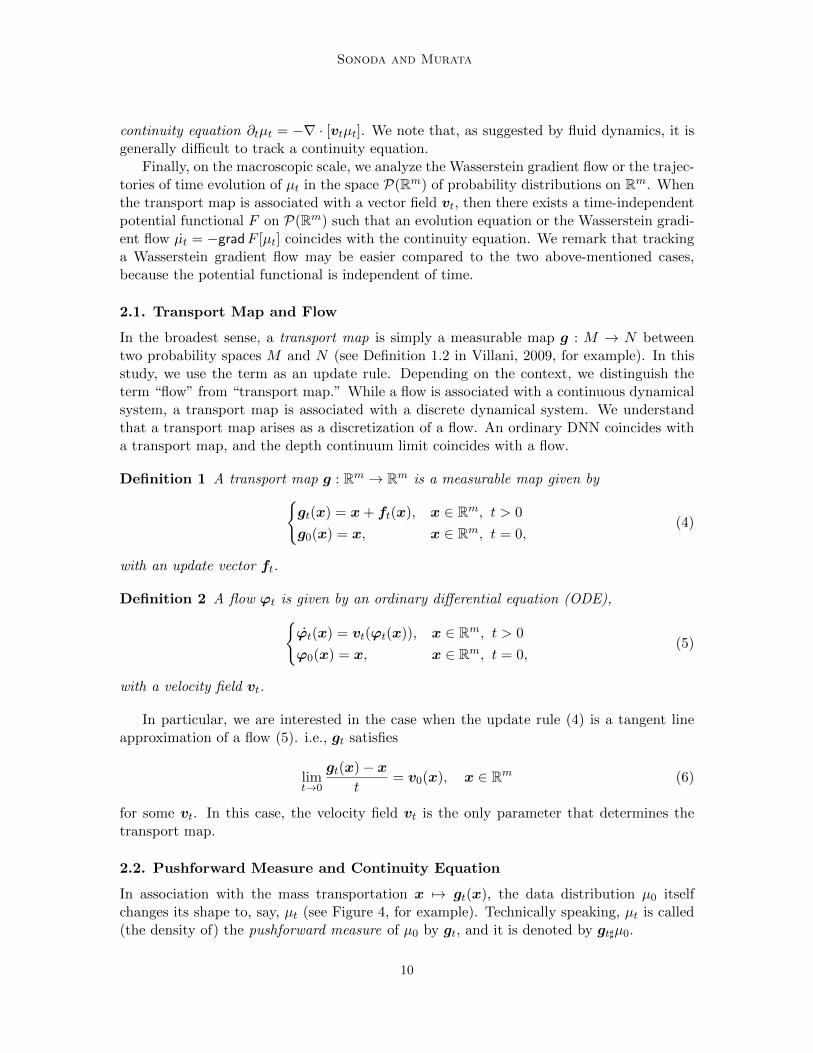
2.1. Transport Map and Flow

In the broadest sense, a transport map is simply a measurable map g : M → N betweentwo probability spaces M and N (see Definition 1.2 in Villani, 2009, for example). In thisstudy, we use the term as an update rule. Depending on the context, we distinguish theterm “flow” from “transport map.” While a flow is associated with a continuous dynamicalsystem, a transport map is associated with a discrete dynamical system. We understandthat a transport map arises as a discretization of a flow. An ordinary DNN coincides witha transport map, and the depth continuum limit coincides with a flow.

Definition 1 A transport map g : Rm → Rm is a measurable map given by

gt(x) = x+ ft(x), x ∈ Rm, t > 0

g0(x) = x, x ∈ Rm, t = 0,(4)

with an update vector ft.

Definition 2 A flow ϕt is given by an ordinary differential equation (ODE),

ϕt(x) = vt(ϕt(x)), x ∈ Rm, t > 0

ϕ0(x) = x, x ∈ Rm, t = 0,(5)

with a velocity field vt.

In particular, we are interested in the case when the update rule (4) is a tangent lineapproximation of a flow (5). i.e., gt satisfies

limt→0

gt(x)− xt

= v0(x), x ∈ Rm (6)

for some vt. In this case, the velocity field vt is the only parameter that determines thetransport map.

2.2. Pushforward Measure and Continuity Equation

In association with the mass transportation x 7→ gt(x), the data distribution µ0 itselfchanges its shape to, say, µt (see Figure 4, for example). Technically speaking, µt is called(the density of) the pushforward measure of µ0 by gt, and it is denoted by gt]µ0.

10


Definition 3 Let µ be a Borel measure on M and g : M → N be a measurable map. Then,g]µ denotes the image measure (or pushforward) of µ by g. It is a measure on N , definedby (g]µ)(B) = µ g−1(B) for every Borel set B ⊂ N .

The pushforward µt is calculated by the change-of-variables formula. In particular,the following extended version by Evans and Gariepy (2015, Theorem 3.9) from geometricmeasure theory is useful.

Fact 1 Let g : Rm → Rn be Lipschitz continuous, m ≤ n, and µ be a probability density onRm. Then, the pushforward g]µ satisfies

g]µ g(x)[∇g](x) = µ(x), a.e.x. (7)

Here, the Jacobian is defined by

[∇g] =√

det |(∇g)∗ (∇g)|. (8)

The continuity equation describes the one-to-one relation between a flow and the push-forward.

Fact 2 Let ϕt be the flow of an ODE (5) with vector field vt. Then, the pushforward µt ofthe initial distribution µ0 evolves according to the continuity equation

∂tµt(x) = −∇ · [µt(x)vt(x)], x ∈ Rm, t ≥ 0. (9)

Here, ∇· denotes the divergence operator in Rm.

The continuity equation is also known as the conservation of mass formula, and this relationbetween the partial differential equation (PDE) (9) and the ODE (5) is a well-known factin continuum physics (Villani, 2009, pp.19). See Appendix B for a sketch of the proof andAmbrosio et al. (2008, § 8) for more detailed discussions.

2.3. Wasserstein Gradient Flow Associated with Continuity Equation

In addition to the ODE and PDE in Rm, we introduce the third profile: the Wassersteingradient flow or the evolution equation in the space of the probability densities on Rm. TheWasserstein gradient flow has a distinct advantage that the potential functional F of thegradient flow is independent of time t; on the other hand, the vector field vt is usually time-dependent. Furthermore, it often facilitates the understanding of transport maps becausewe will see that both the Boltzmann entropy and the Renyi entropy are examples of F .

Let P2(Rm) be the L2-Wasserstein space defined in Section 1.3.3, and let µt ∈ P2(Rm)be the solution of the continuity equation (9) with initial distribution µ0 ∈ P2(Rm). Then,the map t 7→ µt plots a curve in P2(Rm). According to the Otto calculus (Villani, 2009,§ 23), this curve coincides with a functional gradient flow in P2(Rm), called the Wassersteingradient flow, with respect to some potential functional F : P2(Rm)→ R.

Specifically, we further assume that the vector field vt is given by the gradient vectorfield ∇Vt of a potential function Vt : Rm → R.

11

Sonoda and Murata

Fact 3 Assume that µt satisfies the continuity equation with the gradient vector field,

∂tµt = −∇ · [µt∇Vt], (10)

and that we have found F that satisfies the following equation:

d

dtF [µt] =

∫

Rm

∇Vt(x)[∂tµt](x)dx. (11)

Then, the Wasserstein gradient flow

d

dtµt = −gradF [µt], (12)

coincides with the continuous equation.

Here, grad denotes the gradient operator on L2-Wasserstein space P2(Rm) explained inSection 1.3.3. While (12) is an evolution equation or an ODE in P2(Rm), (9) is a PDE inRm. Hence, we use different notations for the time derivatives, d

dt and ∂t.

3. Denoising Autoencoder

We formulate the denoising autoencoder (DAE) as a variational problem, and we showthat the minimizer g∗ or the training result is a transport map. Even though the term“DAE” refers to a training procedure of neural networks, we refer to the minimizer ofDAE also as a “DAE.” We further investigate the initial velocity vector field ∂tgt=0 formass transportation, and we show that the data distribution µt evolves according to thecontinuity equation.

For the sake of simplicity, we assume that the hidden unit number of NNs is sufficientlylarge (or infinite), and thus the NNs can always attain the minimum. Furthermore, weassume the the size of data set is sufficiently large (or infinite). In the case when the hiddenunit number and the size of data set are both finite, we understand the DAE g is composedof the minimizer g∗ and the residual term h. Namely, g = g∗ + h. However, theoreticalinvestigations on the approximation and estimation error h remain as our future work.

3.1. Training Procedure of DAE

Let x be an m-dimensional random vector that is distributed according to the data distri-bution µ0, and let x be its corruption defined by

x = x+ ε, ε ∼ νt

where νt denotes the noise distribution parametrized by variance t ≥ 0. A basic example ofνt is the Gaussian noise with mean 0 and variance t, i.e., νt = N(0, tI).

The DAE is a function that is trained to remove corruption x and restore it to theoriginal x; this is equivalent to finding a function g that minimizes an objective function,i.e.,

L[g] := Ex,x|g(x)− x|2. (13)

12


Note that as long as g is a universal approximator and can thus attain the minimum, itneed not be a neural network. Specifically, our analysis in this section and the next sectionis applicable to a wide range of learning machines. Typical examples of g include neuralnetworks with a sufficiently large number of hidden units, splines (Wahba, 1990), kernelmachines (Shawe-Taylor and Cristianini, 2004) and ensemble models (Schapire and Freund,2012).

3.2. Transport Map of DAE

Theorem 4 (Modification of Theorem 1 by Alain and Bengio, 2014). The global minimumg∗t of L[g] is attained at

g∗t (x) =1

νt ∗ µ0(x)

∫

Rm

xνt(x− x)µ0(x)dx, (14)

= x− 1

νt ∗ µ0(x)

∫

Rm

ενt(ε)µ0(x− ε)dε︸︷︷︸

=:ft(x)

, (15)

where ∗ denotes the convolution operator.

Here, the second equation is simply derived by changing the variable x ← x − ε (seeAppendix A for the complete proof, where we used the calculus of variations). Note thatthis calculation first appeared in Alain and Bengio (2014, Theorem 1), where the authorsobtained (14).

The DAE g∗t (x) is composed of the identity term x and the denoising term ft(x). If weassume that νt → δt as t→ 0, then in the limit t→ 0, the denoising term ft(x) vanishes andDAE reduces to a traditional autoencoder. We reinterpret the DAE g∗t (x) as a transportmap with transport time t that transports the mass at x ∈ Rm toward x+ft(x) ∈ Rm withdisplacement vector ft(x).

3.3. Statistical Interpretation of DAE

In statistics, (15) is known as Brown’s representation of the posterior mean (George et al.,2006). This is not just a coincidence, because the DAE g∗t is an estimator of the mean.Recall that a DAE is trained to retain the original vector x, given its corruption x = x+ε.At least in principle, this is nonsense because to retain x from x means to reverse therandom walk x = x + ε (in Figure 4, the multimodal distributions µ0.5 and µ1.0 indicateits difficulty). Obviously, this is an inverse problem or a statistical estimation problem ofthe latent vector x, given the noised observation x with the observation model x = x+ ε.According to a fundamental fact of estimation theory, the minimum mean squared error(MMSE) estimator of x given x is given by the posterior mean E[x|x]. In our case, theposterior mean equals g∗t .

E[x|x] =

∫Rm xp(x | x)p(x)dx∫Rm p(x | x′)p(x′)dx′

=1

νt ∗ µ0(x)

∫

Rm

xνt(x− x)µ0(x)dx = g∗t (x). (16)

Similarly, we can interpret the denoising term ft(x) as the posterior mean E[ε|x] of noiseε given observation x.

13

Sonoda and Murata

3.4. Examples: Gaussian DAE

When the noise distribution is Gaussian with mean 0 and covariance tI, i.e.,

νt(ε) =1

(2πt)m/2e−|ε|

2/2t,

the transport map is calculated as follows.

Theorem 5 The transport map g∗t of Gaussian DAE is given by

g∗t (x) = x+ t∇ log[νt ∗ µ0](x). (17)

Proof The proof is straightforward by using Stein’s identity,

−t∇νt(ε) = ε νt(ε),

which is known to hold only for Gaussians.

g∗t (x) = x− 1

νt ∗ µ0(x)

∫

Rm

ενt(ε)µ0(x− ε)dε

= x+1

νt ∗ µ0(x)

∫

Rm

t∇νt(ε)µ0(x− ε)dε

= x+t∇νt ∗ µ0(x)

νt ∗ µ0(x)

= x+ t∇ log[νt ∗ µ0(x)].

Theorem 6 At the initial moment t → 0, the pushforward µt of Gaussian DAE satisfiesthe backward heat equation

∂tµt=0(x) = −4µ0(x), x ∈ Rm, (18)

where 4 denotes the Laplacian.

Proof The initial velocity vector is given by the Fisher score

∂tg∗t=0(x) = lim

t→0

g∗t (x)− xt

= ∇ logµ0(x). (19)

Hence, by substituting the score (19) in the continuity equation (9), we have

∂tµt=0(x) = −∇ · [µ0(x)∇ logµ0(x)] = −∇ · [∇µ0(x)] = −4µ0(x).

The backward heat equation (BHE) rarely appears in nature. However, of course, thepresent result is not an error. As mentioned in Section 3.3, the DAE solves an estimationproblem. Therefore, in the sense of the mean, the DAE behaves as time reversal. We remarkthat, as shown by Figure 4, a training result of a DAE with a real NN on a finite data setdoes not converge to a perfect time reversal of a diffusion process.

14


0.0 0.5 1.0 1.5

−3

−2

−1

01

23

t

x

Figure 4: Shallow Gaussian DAE, which is one of the most fundamental versions of DNNs,transports mass, from the left to the right, to decrease the Shannon entropy of data. Thex-axis represents the 1-dimensional input/output space, the t-axis represents the varianceof the Gaussian noise, and t is the transport time. The leftmost distribution depicts theoriginal data distribution µ0 = N(0, 1). The middle and rightmost distributions depictthe pushforward µt = gt]µ0, associated with the transportation by two DAEs with noisevariance t = 0.5 and t = 1.0, respectively. As t increases, the variance of the pushforwarddecreases.

4. Deep DAEs

We introduce the composition gL · · · g0 of DAEs g` : Rm → Rm and its continuum limit:the continuous DAE ϕt : Rm → Rm. We can understand the composition of DAEs as theEuler scheme or the broken line approximation of a continuous DAE.

For the sake of simplicity, we assume that the hidden unit number of NNs is infinite,and that the size of data set is infinite.

4.1. Composition of DAEs

We write 0 = t0 < t1 < · · · < tL+1 = t. We assume that the input vector x0 ∈ Rm is subjectto a data distribution µ0. Let g0 : Rm → Rm be a DAE that is trained on µ0 with noisevariance t1 − t0. Then, let x1 := g0(x0), which is a random vector in Rm that is subjectto the pushforward µ1 := g0]µ0. We train another DAE g1 : Rm → Rm on µ1 with noisevariance t2− t1. By repeating the procedure, we obtain g`(x`) from x`−1 that is subject toµ` := g(`−1)]µ`−1.

For the sake of generality, we assume that each component DAE is given by

g`(x) = x+ (t`+1 − t`)∇Vt`(x), (` = 0, . . . , L) (20)

15

Sonoda and Murata

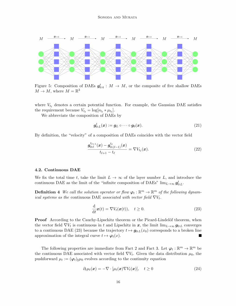
M M M M M Mg`=0 g`=1 g`=2 g`=3 g`=4

Figure 5: Composition of DAEs gt0:4 : M → M , or the composite of five shallow DAEsM →M , where M = R3

where Vt` denotes a certain potential function. For example, the Gaussian DAE satisfiesthe requirement because Vt` = log[νt` ∗ µt` ].

We abbreviate the composition of DAEs by

gt0:L(x) := gL · · · g0(x). (21)

By definition, the “velocity” of a composition of DAEs coincides with the vector field

gt`+1

0:` (x)− gt`0:(`−1)(x)

t`+1 − t`= ∇Vt`(x). (22)

4.2. Continuous DAE

We fix the total time t, take the limit L → ∞ of the layer number L, and introduce thecontinuous DAE as the limit of the “infinite composition of DAEs” limL→∞ g

t0:L.

Definition 4 We call the solution operator or flow ϕt : Rm → Rm of the following dynam-ical systems as the continuous DAE associated with vector field ∇Vt.

d

dtx(t) = ∇Vt(x(t)), t ≥ 0. (23)

Proof According to the Cauchy-Lipschitz theorem or the Picard-Lindelof theorem, whenthe vector field ∇Vt is continuous in t and Lipschitz in x, the limit limL→∞ g0:L convergesto a continuous DAE (23) because the trajectory t 7→ g0:L(x0) corresponds to a broken lineapproximation of the integral curve t 7→ ϕt(x).

The following properties are immediate from Fact 2 and Fact 3. Let ϕt : Rm → Rm bethe continuous DAE associated with vector field ∇Vt. Given the data distribution µ0, thepushforward µt := (ϕt)]µ0 evolves according to the continuity equation

∂tµt(x) = −∇ · [µt(x)∇Vt(x)], t ≥ 0 (24)

16


and the Wasserstein gradient flow

d

dtµt = −gradF [µt], t ≥ 0 (25)

where F is given by (11).

4.3. Example: Gaussian DAE

We consider a continuous Gaussian DAE ϕt trained on µ0 ∈ P2(Rm). Specifically, it satisfies

d

dtx(t) = ∇ log[µt(x(t))], t ≥ 0 (26)

with µt := ϕt]µ0.

Theorem 7 The pushforward µt := ϕt]µ0 of the continuous Gaussian DAE ϕt is the so-lution to the initial value problem of the backward heat equation (BHE)

∂tµt(x) = −4µt(x), µt=0(x) = µ0(x). (27)

The proof is immediate from Theorem 6.

As mentioned after Theorem 6, the BHE appears because the DAE solves an estimationproblem. We remark that the BHE is equivalent to the following final value problem for theordinary heat equation:

∂tut(x) = 4ut(x), ut=T (x) = µ0(x) for some T

where ut denotes a probability measure on Rm. Indeed, µt(x) = uT−t(x) solves (27). Inother words, the backward heat equation describes the time reversal of an ordinary diffusionprocess.

According to Wasserstein geometry, an ordinary heat equation corresponds to a Wasser-stein gradient flow that increases the Shannon entropy functionalH[µ] := −

∫µ(x) logµ(x)dx

(Villani, 2009, Th. 23.19). Consequently, we can conclude that the continuous GaussianDAE is a transport map that decreases the Shannon entropy of the data distribution.

Theorem 8 The pushforward µt := ϕt]µ0 evolves according to the Wasserstein gradientflow with respect to the Shannon entropy

d

dtµt = −gradH[µt], µt=0 = µ0. (28)

Proof When F = H, then Vt = − logµt; thus,

gradH[µt] = ∇ · [µt∇ logµt] = ∇ · [∇µt] = 4µt,

which means that the continuity equation reduces to the backward heat equation.

17

Sonoda and Murata

4.4. Example: Renyi Entropy

Similarly, when F is the Renyi entropy

Hα[µ] :=

∫

Rm

µα(x)− µ(x)

α− 1dx,

then gradHα[µt] = 4µαt (see Ex. 15.6 in Villani, 2009, for the proof) and thus the continuityequation reduces to the backward porous medium equation

∂tµt(x) = −4µαt (x). (29)

5. Further Investigations on Shallow and Deep DAEs through Examples

5.1. Analytic Examples

We list analytic examples of shallow and continuous DAEs (see Appendix D for furtherdetails, including proofs). In all the settings, the continuous DAEs attain a singular measureat some finite t > 0 with various singular supports that reflect the initial data distributionµ0, while the shallow DAEs accept any t > 0 and degenerate to a point mass as t→∞.

5.1.1. Univariate Normal Distribution

When the data distribution is a univariate normal distribution N(m0, σ0), the transportmap and pushforward for the shallow DAE are given by

gt(x) =σ2

0

σ20 + t

x+t

σ20 + t

m0, (30)

µt = N

(m0,

σ20

(1 + t/σ20)2

), (31)

and those of the continuous DAE are given by

gt(x) =√

1− 2t/σ20(x−m0) +m0, (32)

µt = N(m0, σ20 − 2t). (33)

5.1.2. Multivariate Normal Distribution

When the data distribution is a multivariate normal distribution N(m0,Σ0), the transportmap and pushforward for the shallow DAE are given by

gt(x) = (I + tΣ−10 )−1x+ (I + t−1Σ0)−1m0, (34)

µt = N(m0,Σ0(I + tΣ−10 )−2), (35)


gt(x) =

√I − 2tΣ−1

0 (x−m0) +m0, (36)

µt = N(m0,Σ0 − 2tI). (37)

18


5.1.3. Mixture of Multivariate Normal Distributions

When the data distribution is a mixture of multivariate normal distributions∑K

k=1wkN(mk,Σk)with the assumption that it is well separated, the transport map and pushforward for theshallow DAE are given by

gt(x) =K∑

k=1

γkt(x)

(I + tΣ−1k )−1x+ (I + t−1Σk)

−1mk

, (38)

µt ≈K∑

k=1

wkN(mk,Σk(I + tΣ−1k )−2), (39)

with responsibility function

γkt(x) :=wkN(x;mk,Σk + tI)

∑Kk=1wkN(x;mk,Σk + tI)

, (40)


gt(x) ≈√I − 2tΣ−1

k (x−mk) +mk, (41)

µt =K∑

k=1

wkN(mk,Σk − 2tI), (42)

with responsibility function

γkt(x) :=wkN(x;mk,Σk − 2tI)

∑Kk=1wkN(x;mk,Σk − 2tI)

. (43)

Here, we say that the mixture∑K

k=1wkN(mk,Σk) is well separated when for every clustercenter mk, there exists a neighborhood Ωk of mk such that N(Ωk;mk,Σk) ≈ 1 and γkt ≈1Ωk

.

5.2. Numerical Example of Trajectories

We employed 2-dimensional examples, in order to visualize the difference of vector fields be-tween the shallow and deep DAEs. In the examples below, every trajectories are drawn intoattractors, however the shape of the attractors and the speed of trajectories are significantlydifferent between shallow and deep.

5.2.1. Bivariate Normal Distribution

Figure 6 compares the trajectories of four DAEs trained on the common data distribution

µ0 = N

([0, 0],

[2 00 1

]). (44)

The transport maps for computing the trajectories are given by (34) for the shallow DAEand composition of DAEs, and by (36) for the continuous DAE. Here, we applied (34)multiple times for the composition of DAEs.

19

Sonoda and Murata

The continuous DAE converges to an attractor lying on the x-axis at t = 1/2. Bycontrast, the shallow DAE slows down as t→∞ and never attains the singularity in finitetime. As L tends to infinity, gt0:L plots a trajectory similar to that of the continuous DAEϕt; the curvature of the trajectory changes according to ∆t.

5.2.2. Mixture of Bivariate Normal Distributions

Figure 7, 8, and 9 compare the trajectories of four DAEs trained on the three common datadistributions

µ0 = 0.5N

([−1, 0],

[1 00 1

])+ 0.5N

([1, 0],

[1 00 1

]), (45)

µ0 = 0.2N

([−1, 0],

[1 00 1

])+ 0.8N

([1, 0],

[1 00 1

]), (46)

µ0 = 0.2N

([−1, 0],

[1 00 1

])+ 0.8N

([1, 0],

[2 00 1

]). (47)

respectively.The transport maps for computing the trajectories are given by (38) for the shallow

DAE and composition of DAEs. For the continuous DAE, we compute the trajectories bynumerically solving the definition of the continuous Gaussian DAE: x = ∇ logµt(x).

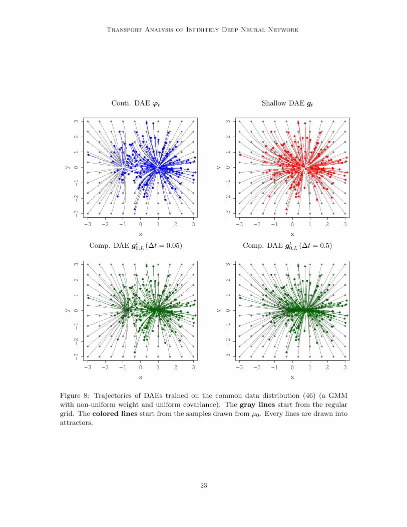
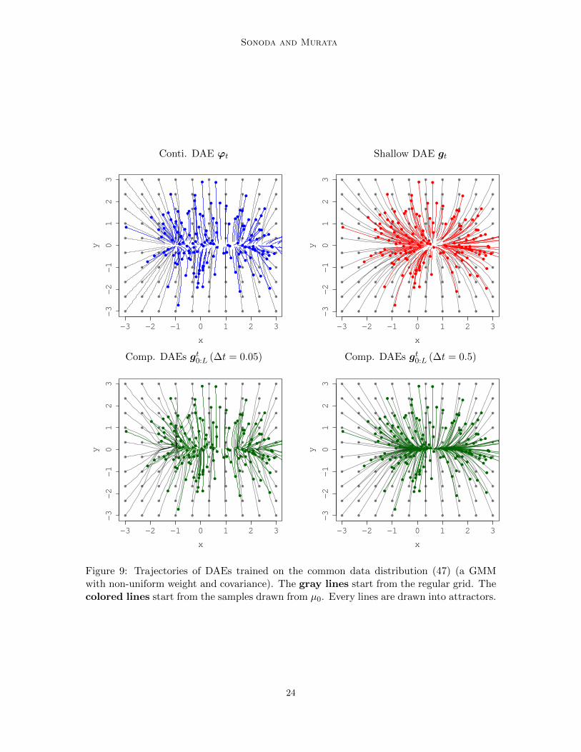
In any case, the continuous DAE converges to an attractor at some t > 0, but theshape of the attractors and the basins of attraction change according to the initial datadistribution. The shallow DAE converges to the origin as t → ∞, and the composition ofDAEs plots a curve similar to that of the continuous DAE as L tends to infinity, gt0:L. Inparticular, in Figure 8, some trajectories of the continuous DAE intersect, which impliesthat the velocity vector field vt is time-dependent.

20


Conti DAE ϕt

−3 −2 −1 0 1 2 3

−3

−2

−1

01

23

x

y

Shallow DAE gt

−3 −2 −1 0 1 2 3−

3−

2−

10

12

3x

y

Comp. DAE gt0:L (∆t = 0.05)

−3 −2 −1 0 1 2 3

−3

−2

−1

01

23

x

y


−3 −2 −1 0 1 2 3

−3

−2

−1

01

23

x

y

Figure 6: Trajectories of DAEs trained on the common data distribution (44) (µ0 =N([0, 0], diag [2, 1])). The gray lines start from the regular grid. The colored lines startfrom the samples drawn from µ0. The midpoints are plotted every ∆t = 0.2. Every linesare drawn into attractors.

21

Sonoda and Murata

Conti DAE ϕt

−3 −2 −1 0 1 2 3

−3

−2

−1

01

23

x

y

Shallow DAE gt

−3 −2 −1 0 1 2 3−

3−

2−

10

12

3

x

y


−3 −2 −1 0 1 2 3

−3

−2

−1

01

23

x

y


−3 −2 −1 0 1 2 3

−3

−2

−1

01

23

x

y

Figure 7: Trajectories of DAEs trained on the common data distribution (45) (a GMM withuniform weight and covariance). The gray lines start from the regular grid. The coloredlines start from the samples drawn from µ0. Every lines are drawn into attractors.

22


Conti. DAE ϕt

−3 −2 −1 0 1 2 3

−3

−2

−1

01

23

x

y

Shallow DAE gt

−3 −2 −1 0 1 2 3−

3−

2−

10

12

3x

y


−3 −2 −1 0 1 2 3

−3

−2

−1

01

23

x

y


−3 −2 −1 0 1 2 3

−3

−2

−1

01

23

x

y

Figure 8: Trajectories of DAEs trained on the common data distribution (46) (a GMMwith non-uniform weight and uniform covariance). The gray lines start from the regulargrid. The colored lines start from the samples drawn from µ0. Every lines are drawn intoattractors.

23

Sonoda and Murata

Conti. DAE ϕt

−3 −2 −1 0 1 2 3

−3

−2

−1

01

23

x

y

Shallow DAE gt

−3 −2 −1 0 1 2 3−

3−

2−

10

12

3

x

y

Comp. DAEs gt0:L (∆t = 0.05)

−3 −2 −1 0 1 2 3

−3

−2

−1

01

23

x

y

Comp. DAEs gt0:L (∆t = 0.5)

−3 −2 −1 0 1 2 3

−3

−2

−1

01

23

x

y

Figure 9: Trajectories of DAEs trained on the common data distribution (47) (a GMMwith non-uniform weight and covariance). The gray lines start from the regular grid. Thecolored lines start from the samples drawn from µ0. Every lines are drawn into attractors.

24


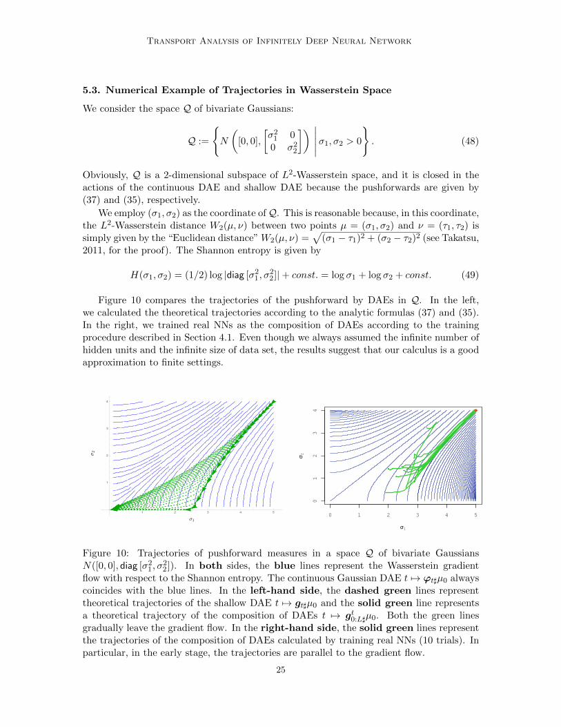
5.3. Numerical Example of Trajectories in Wasserstein Space

We consider the space Q of bivariate Gaussians:

Q :=

N

([0, 0],

[σ2

1 00 σ2

2

]) ∣∣∣∣∣σ1, σ2 > 0

. (48)

Obviously, Q is a 2-dimensional subspace of L2-Wasserstein space, and it is closed in theactions of the continuous DAE and shallow DAE because the pushforwards are given by(37) and (35), respectively.

We employ (σ1, σ2) as the coordinate ofQ. This is reasonable because, in this coordinate,the L2-Wasserstein distance W2(µ, ν) between two points µ = (σ1, σ2) and ν = (τ1, τ2) issimply given by the “Euclidean distance”W2(µ, ν) =

√(σ1 − τ1)2 + (σ2 − τ2)2 (see Takatsu,

2011, for the proof). The Shannon entropy is given by

H(σ1, σ2) = (1/2) log |diag [σ21, σ

22]|+ const. = log σ1 + log σ2 + const. (49)

Figure 10 compares the trajectories of the pushforward by DAEs in Q. In the left,we calculated the theoretical trajectories according to the analytic formulas (37) and (35).In the right, we trained real NNs as the composition of DAEs according to the trainingprocedure described in Section 4.1. Even though we always assumed the infinite number ofhidden units and the infinite size of data set, the results suggest that our calculus is a goodapproximation to finite settings.

σ2

1 2 3 4 5

1

2

3

4

σ1

0 1 2 3 4 5

01

23

4

σ1

σ 2

Figure 10: Trajectories of pushforward measures in a space Q of bivariate GaussiansN([0, 0], diag [σ2

1, σ22]). In both sides, the blue lines represent the Wasserstein gradient

flow with respect to the Shannon entropy. The continuous Gaussian DAE t 7→ ϕt]µ0 alwayscoincides with the blue lines. In the left-hand side, the dashed green lines representtheoretical trajectories of the shallow DAE t 7→ gt]µ0 and the solid green line representsa theoretical trajectory of the composition of DAEs t 7→ gt0:L]µ0. Both the green linesgradually leave the gradient flow. In the right-hand side, the solid green lines representthe trajectories of the composition of DAEs calculated by training real NNs (10 trials). Inparticular, in the early stage, the trajectories are parallel to the gradient flow.

25

Sonoda and Murata

6. Equivalence between Stacked DAE and Compositions of DAEs

As an application of transport analysis, we shed light on the equivalence of the stacked DAE(SDAE) and the composition of DAEs (CDAE), provided that the definition of DAEs isgeneralized to L-DAE, which is defined below. In SDAE, we apply the DAE to the featuresvectors obtained from the hidden layer of an NN to obtain higher-order feature vectors.Therefore, the feature vectors obtained from the SDAE and CDAE are different from eachother. Nevertheless, we can prove that the trajectories generated by the SDAE and CDAEare topologically conjugate, which means that there exists a homeomorphism between thetrajectories. Moreover, we can transform the trajectory of an SDAE into that of a CDAEby using a linear map, which is obtained from the decoder of the SDAE. Thus, we cansynthesize the feature vectors of the SDAE by using CDAEs.

6.1. Definitions

To begin with, we introduce a generalized version of shallow DAE.

Definition 5 (L-DAE) Let L be an elliptic operator on the domain Ω in Rm, µ be aprobability density on Ω, and D be a positive definite matrix. The L-DAE with diffusioncoefficient D and initial data µ is defined by

id + tD∇ log etLµ, t > 0. (50)

Here, etL is the semigroup generated by the elliptic operator L. Specifically, let µt :=etLµ; then, µt satisfies the parabolic equation ∂tµt = Lµt. The original Gaussian DAEcorresponds to a special case when D ≡ I and L = 4.

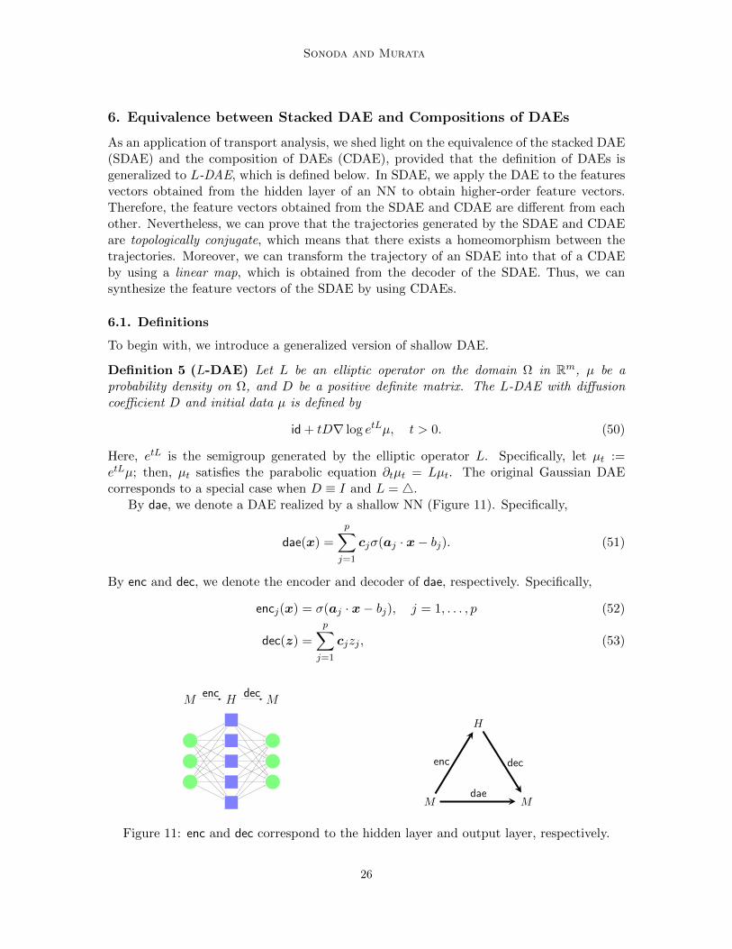
By dae, we denote a DAE realized by a shallow NN (Figure 11). Specifically,

dae(x) =

p∑

j=1

cjσ(aj · x− bj). (51)

By enc and dec, we denote the encoder and decoder of dae, respectively. Specifically,

encj(x) = σ(aj · x− bj), j = 1, . . . , p (52)

dec(z) =

p∑

j=1

cjzj , (53)

M H Menc dec

M M

H

enc

dae

dec

Figure 11: enc and dec correspond to the hidden layer and output layer, respectively.

26


where zj denotes the j-th element of z = enc(x). Obviously, dae = dec enc.For the sake of simipicity, even though we introduced the finite number p of hidden

units, we assume that p is large, and thus dae approximately equals L-DAE for some L.

6.2. Training Procedure of Stacked DAE (SDAE)

Let M := Rm be the space of input vectors with probability density µ, and let dae : M →Mbe a shallow NN with p hidden units. We assume that dae is trained as the Gaussian DAEwith µ, and it thus approximates the DAE id + t∇ log[et4µ]. Let H := Rp. Then, theencoder and decoder of dae are the maps enc : M → H and dec : H →M , respectively.

In the SDAE, we apply the DAE to z. Specifically, let µ be the density of hidden featurevectors z = enc(x), and let dae : H → H be a shallow NN with p hidden units,

dae(z) :=

p∑

=1

cσ(a · z − b).

We train dae by using the Gaussian DAE with µ, where the network is decomposed asdae = dec enc with enc : H → H and dec : H → H, and we obtain the feature vectorsz := enc(z) ∈ H = Rp. By iterating the stacking procedure, we can obtain more abstractfeature vectors (Figure 12).

H H Henc dec

M M

H H

H

enc

dae

dec

enc

dae

dec

Figure 12: The (feature map of) SDAE enc enc is built on the hidden layer.

Technically speaking, µ is (the density of) the pushforward dae]µ, and its support is

contained in the image M := enc(M). In general, we assume that dim M(= dimM) ≤dimH; thus, the support of µ is singular (i.e., the density vanishes outside M) (see Fact 1for further details).

6.3. Topological Conjugacy

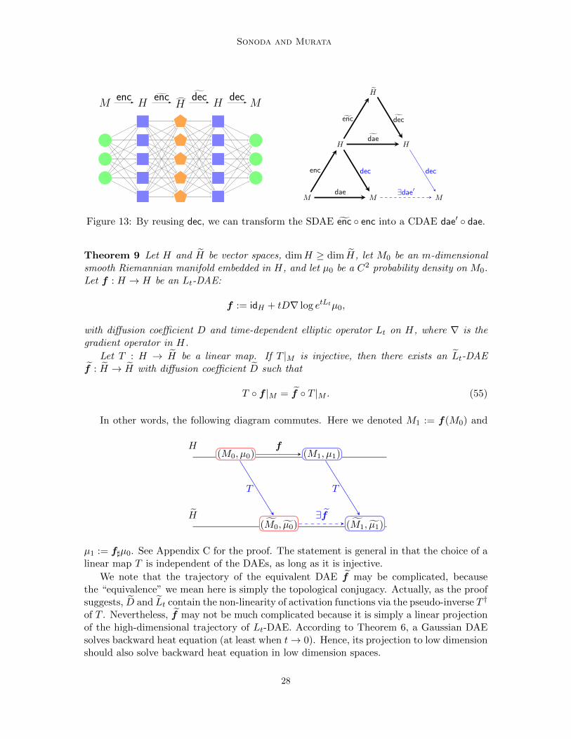
The transport map of the feature vector enc enc : M → H → H is somewhat unclear.According to Theorem 9 and 10, the transport map of enc enc can be transformed orprojected to the ground space M by applying dec dec (Figure 13). Specifically, there existsan L-DAE dae′ : M →M such that

dec dec enc enc = dae′ dae. (54)

27

Sonoda and Murata

M H H H Menc enc dec dec

M M

H

M

H

H

enc

dae

dec

enc

dae

dec

dec

∃dae′

Figure 13: By reusing dec, we can transform the SDAE enc enc into a CDAE dae′ dae.

Theorem 9 Let H and H be vector spaces, dimH ≥ dim H, let M0 be an m-dimensionalsmooth Riemannian manifold embedded in H, and let µ0 be a C2 probability density on M0.Let f : H → H be an Lt-DAE:

f := idH + tD∇ log etLtµ0,

with diffusion coefficient D and time-dependent elliptic operator Lt on H, where ∇ is thegradient operator in H.

Let T : H → H be a linear map. If T |M is injective, then there exists an Lt-DAEf : H → H with diffusion coefficient D such that

T f |M = f T |M . (55)

In other words, the following diagram commutes. Here we denoted M1 := f(M0) and

H

H

(M0, µ0)

(M0, µ0)

(M1, µ1)

(M1, µ1)

T T

f

∃f

µ1 := f]µ0. See Appendix C for the proof. The statement is general in that the choice of alinear map T is independent of the DAEs, as long as it is injective.

We note that the trajectory of the equivalent DAE f may be complicated, becausethe “equivalence” we mean here is simply the topological conjugacy. Actually, as the proofsuggests, D and Lt contain the non-linearity of activation functions via the pseudo-inverse T †

of T . Nevertheless, f may not be much complicated because it is simply a linear projectionof the high-dimensional trajectory of Lt-DAE. According to Theorem 6, a Gaussian DAEsolves backward heat equation (at least when t→ 0). Hence, its projection to low dimensionshould also solve backward heat equation in low dimension spaces.

28


6.4. Equivalence between SDAE and CDAE

To clarify the statement, we prepare the notation. Figure 14 summarizes the symbols andprocedures.

First, we rewrite the input vector as z0 instead of x, the input space as H0 = M00 (=

Rm) instead of M , and the density as µ00 instead of µ. We iteratively train the `-th NN

dae`` : H` → H` with a data distribution µ``, obtain the encoder enc` : H` → H`+1 anddecoder dec` : H`+1 → H`, and update the feature z`+1 := enc`(z`), the image M `+1

`+1 :=

enc`(M `` ) ⊂ H`+1, and the distribution µ`+1

`+1 := (enc`)]µ`µ.

For simplicity, we abbreviate

enc`:n := encn · · · enc`,decn:` := dec` · · · decn.

In addition, we introduce auxiliary objects.

Mn`+1 := dec`:n(M `+1

`+1 ), n = 0, · · · , `µn`+1 := dec`:n] µ`+1

`+1, n = 0, · · · , `.

By construction, M `n is an at most m-dimensional submanifold in H`, and the support of

µ`n is in M `n.

Finally, we denote the map dae`n : M `n → M `

n+1 that is (not “trained by DAE” but)defined by

dae`n := (decn:` enc0:n) (dec(n−1):` enc0:(n−1))−1 : M `n →M `

n+1.

By Theorem 9, if dae`+1n is an L`+1

n -DAE, then dae`n exists and it is an L`n-DAE.

Theorem 10 If every enc`|M``

is a continuous injection and every dec`|M`+1n

is an injection,

then

decL:0 enc0:L = dae0L · · · dae0

0. (56)

Proof By repeatedly applying the topological conjugacy in Theorem 9,

dec` dae`+1n = dae`n dec`,

we have

decL:0 enc0:L

= dec(L−2):0 decL−1 daeLL encL−1 enc0:(L−2)

= dec(L−2):0 daeL−1L decL−1 encL−1 enc0:(L−2)

= dec(L−2):0 daeL−1L daeL−1

L−1 enc0:(L−2)

· · ·= dae0

L dae0L−1 · · · dae0

0.

29

Sonoda and Murata

H0 = M

H1

H2

HL

HL+1

(M00 , µ

00) (M0

1 , µ01)

(M11 , µ

11)

(M02 , µ

02)

(M12 , µ

12)

(M22 , µ

22)

(M03 , µ

03)

(M13 , µ

13)

(M23 , µ

23)

(MLL , µ

LL)

(M0L+1, µ

0L+1)

(M1L+1, µ

1L+1)

(M2L+1, µ

2L+1)

(MLL+1, µ

LL+1)

(ML+1L+1 , µ

L+1L+1)

(MLL , µ

LL)

enc0 dec0

dae00

enc1 dec1

dae11

dae22

encL decL

daeLL

‖

dec0

dae01

dec0

dae02

dec0

dae0L

dec1

dae12

dec1

dae1L

dae2L‖‖

‖

‖

‖

Figure 14: By using decoders, an SDAE is transformed or projected into a CDAE. Theleftmost arrows correspond to the SDAE enc0:L, the rightmost arrows correspond to thedecoders decL:0, and the bottom arrows correspond to the CDAE dae0

L · · · dae00.

6.5. Numerical Example

Figure 15 compares the transportation results of the 2-dimensional swissroll data by theDAEs. In both the cases, the swissroll becomes thinner by the action of transportation. Weremark that to test the topological conjugacy by numerical experiments is difficult. Here,we display Figure 15 to see typical trajectories by an SDAE and a CDAE.

In the left-hand side, we trained an SDAE enc1 enc0 by using real NNs. Specifically, wefirst trained a shallow DAE dae0

0 on the swissroll data x0. Second, writing dae00 = dec0enc0

and letting z1 := enc0(x0), we trained a shallow DAE dae11 on the feature vectors z1. Then,

writing dae11 = dec1 enc1, we obtained x1 := dae0

0(x0) and x2 := dec0 dec1 enc1 enc0.The black points represent the input vectors x0, and the red and blue points representthe first and second transportation results x1 and x2, respectively. In other words, thedistribution of x0,x1 and x2 correspond to µ0

0, µ01 and µ0

2 in Figure 14, respectively.

In the right-hand side, we trained a CDAE dae10dae0

0 by using real NNs. Specifically, wefirst trained a shallow DAE dae0

0 on the swissroll data x0. Second, writing x1 := dae00(x0),

we trained a shallow DAE dae01 on the transported vectors x0

1. Then, we obtained x2 :=dae1

0(x1) = dae10 dae0

0(x0). The black points represent the input vectors x0, and the redand blue points represent the first and second transportation results x1 and x2, respectively.

30


−10 −5 0 5 10 15

−1

5−

10

−5

05

10

15

−10 −5 0 5 10 15

−1

0−

50

51

01

5

Figure 15: Typical transportation results of the 2-dimensional swissroll data by an SDAE(left) and a CDAE (right). In both the sides, the black points represent the input vectorsx0 ∈ R2, and the red and blue points represent the first and second transportation resultsx1 and x2, respectively.

7. Integral Representation of the Flow Representation

In this section, we aim to develop the double continuum limit: a combination of the depthcontinuum limit, or the flow representation, and the width continuum limit, or the integralrepresentation.

To facilitate visualization, we write the hidden parameters as θ instead of (a, b), thek-th element of the coefficient function as γ(θ, k) or γk(θ) instead of the boldface γ(θ), andthe integral representation as

S[γk](x) =

∫γ(θ, k)σ(x;θ)dθ. (57)

Furthermore, by using a singular measure γpk(θ) :=∑p

j=1 cjkδθj (θ), we write an ordinaryshallow NN as

S[γpk ](x) =

∫γp(θ, k)σ(x;θ)dθ =

p∑

j=1

cjkσ(x;θj). (58)

If there is no risk of confusion, we omit writing the superscript p. Specifically, we write“S[γk]” without distinction between an infinite NN (57) and a finite NN (58).

31

Sonoda and Murata

7.1. Encoder and Decoder in the Integral Representation

First, we consider a finite case. Suppose that a shallow DAE is realized by a finite NN∑pj=1 cjkσ(x;θj). Then, the encoder is given by

z(θj) = enc(x,θj) = σ(x;θj), j = 1, . . . , p;

and the decoder is given by

dec(z, k) =

p∑

j=1

cjkz(θj).

Therefore, supposing that a shallow DAE is realized by S[γ], the encoder and decoderin the integral representation are given by

enc(x,θ) := σ(x;θ), (59)

dec(z, k) :=

∫γ(θ, k)z(θ)dθ, (60)

where “the θ-th element” of z is given by z(θ).Next, we consider the stacked DAE built on z. Suppose that the stacked DAE is realized

by S[γθ](z) =∫γ(ω,θ)σ(z;ω)dω; then, the encoder and decoder are given by

enc(z,ω) := σ(z;ω), (61)

dec(u,θ) :=

∫γ(ω,θ)u(ω)dω, (62)

where the ω-th element of u is given by u(ω), and the θ-th element of ω is given by ω(θ).In this notation, for example, the topological conjugacy (55) claims that there exists γ′

such that∫γ(θ, k)

∫γ(ω,θ)σ(σ(x; ·);ω)dωdθ =

∫γ′(θ′, k)σ

(∫γ(θ, ·)σ(x;θ)dθ;θ′

)dθ′. (63)

7.2. Ridgelet Transform of Flows

Let ϕt : Rm → Rm be a flow that satisfies ϕt ϕs = ϕt+s. Then, the following formulaholds:

∫R[ϕt](θ, k)σ

(∫R[ϕs](θ, ·)σ(x;θ′)dθ′

)dθ =

∫R[ϕt+s](θ, k)σ(x;θ)dθ. (64)

In other words, S[R[ϕt]] S[R[ϕs]] = S[R[ϕt+s]]. According to Barron’s bound (Kurkova,2012, Cor.5.4), the discretization error ‖S[γ]− S[γp]‖2 between S[γ] and S[γp] is boundedby ‖γ‖1/√p. Hence, ‖R[ϕt]‖1 + ‖R[ϕs]‖1 ≤ ‖R[ϕt+s]‖1 for some t and s, which implies theexpressive efficiency of the DNN.

Consider a special case when ϕ : Rm → Rm is given by the gradient of a potentialfunction V . Specifically, ϕ = ∇V . We note that according to the polar decompositiontheorem by Brenier (1991), any optimal transport map ϕt : [0, 1] × Rm → Rm can bewritten as ϕt = id+ t∇U with some potential function U . Hence, by letting V = | · |2/2+U ,we can understand ϕ := ϕ1 = ∇V as an optimal transport map.

Then, we have an integration-by-parts formula for the vector ridgelet transform.

32


Theorem 11 Let K ⊂ Rm be a compact set with smooth boundary ∂K. Given that asmooth scalar potential V is supported in K, the ridgelet transform of the potential vectorfield ∇V is calculated by

Rρ[∇V ](a, b) = −aRρ′ [V ](a, b). (65)

Here, Rρ and Rρ′ denote the ridgelet transform with respect to ρ and ρ′, respectively.

Proof

Rρ[∇V ](a, b) =

∫

K∇V (x)ρ(a · x− b)dx

=

[∫

∂KV (x)ρ(a · x− b)n(x)dS − a

∫

KV (x)ρ′(a · x− b)dx

]

= 0− aRρ′ [V ](a, b).

The left-hand side (LHS) of (65) denotes a vector ridgelet transform defined by element-wisemapping, whereas the right-hand side (RHS) consists of a scalar ridgelet transform. We canunderstand the RHS given that the network shares common knowledge among element-wisetasks.

7.3. Example: Autoencoder

As the most fundamental transport map, we consider a smooth “truncated” autoencoderidr,δ. We denote by Bm(z; r) a closed ball in Rm with center z and radius r. We assumethat idr,δ is (1) smooth, (2) equal to the identity map id when it is restricted to Bm(r), and(3) truncated to be supported in Bm(r + δ) with a small positive number δ > 0. Let ∇Vr,δbe a smooth function that satisfies

Vr,δ(x) :=

12 |x|2 x ∈ Bm(0; r),

(smooth map) x ∈ B(0; r + δ) \ B(0; r),

0 x /∈ Bm(0; r + δ),

and let

idr,δ := ∇Vr,δ.

Note that we can construct idr,δ and ∇Vr,δ by using mollifiers; thus, such maps exist.The ridgelet transform of the truncated autoencoder is given by

Rρ[idr,δ](a, b) ≈ −Kaρ′(−b) as δ → 0 (66)

with a certain constant K (see Appendix E for the proof).

33

Sonoda and Murata

8. Discussion

We performed transport analysis of denoising autoencoders by introducing the flow repre-sentation. The flow representation ϕt is the depth continuum limit of a DNN, specifiedby an ODE with vector field vt. We interpreted an ordinary DNN gt as a transport mapor an Euler broken line approximation of ϕt. The advantages of the flow representationare that it provides the coordinate-free treatment of DNNs, avoiding the redundancy ofthe ordinary parametrization of DNNs, and that it facilitates our understanding of whatDNNs do—it is the mass transportation controlled by vt. In addition, the advantage of theinterpretation as mass transportation is that it can handle function composition. In thetransport analysis, we analyzed a flow in three aspects: a dynamical system described by atransport map or vector field, a pushforward measure described by a continuity equation,and Wasserstein gradient flow. From the results in Wasserstein geometry, these aspectsare closely connected, and the hyperparameter vt plays a central role as an intermediary.For example, in the transport analysis of continuous DAEs, the potential functional of theWasserstein gradient flow often facilitates our understanding of the flow because it is theShannon entropy, which is a fundamental quantity in statistics and machine learning.

In Section 3 and 4, we specified the transport maps of shallow, deep, and infinitely deepDAEs, and we gave their statistical interpretations. The shallow DAE is an estimator of themean, while the deep DAE transports data points to decrease the Shannon entropy of thedata distribution, which gives a partial answer to our research question “what do hiddenlayers do?” In Section 5, according to analytic and numerical experiments, we showed thatdeep DAEs converge faster and that the extracted features are different from each other,which gives a partial answer to the other question “why do DNNs perform better?” InSection 6, we proved the equivalence between the stacked DAE and the composition ofDAEs. Because of the peculiar construction, it is difficult to formulate and understandstacking. Nevertheless, by tracking the flow, we succeeded in formulating the stacked DAE.In Section 7, we developed the double continuum limits, or the width continuum limit ofthe depth continuum limit. We presented some examples of the integral representation ofthe flow, such as encoder, decoder, and traditional autoencoder.

As a consequence of the equivalence, we can understand the so-called pre-training andfine-tuning strategy (Bengio et al., 2007; Erhan et al., 2010) as an optimal control problem.Namely, write a DNN as a composite ψ ϕt of classifier ψ : Rm → [0, 1]n and flow ϕt :Rm → Rm. If ϕt stays closer to the identity, ψ has to be more complex—and vice versa.The pre-training regularizes the behavior of hidden layers by

d

dtϕt(x) = vt(ϕt(x)), x ∈ Rm, t > 0 (67)

and the fine-tuning specifies the relation between input and output by

Minimize EX,Y |Y −ψ ϕt=1(X)|2 w.r.t NN ψ ϕt=1. (68)

Overall, we can understand the strategy as the control problem of system (67) under re-striction (68). Owing to ridgelet transform, shallow NNs are interpretable and principled.Development of a “solution operator” to the control problem in the flow representationwould open the way to the interpretable and principled alternative to DNNs.

34


Acknowledgments

The authors thank the editor and reviewers for their supportive and insightful comments,which have improved the clarity of the argument significantly. The authors also acknowl-edge fruitful discussions with Dr. Shotaro Akaho, Dr. Kohei Yatabe, Dr. Keisuke Yano,and Mr. Kentaro Minami. This work was supported by JSPS KAKENHI (15J07517 and18K18113).

Appendix A. Proof of Theorem 4

By L1loc(Rm) and C∞c (Rm), we denote the spaces of locally integrable functions and com-

pactly supported smooth functions, respectively. We assume that g : Rm → Rm is locallyintegrable (L1

loc).Proof The proof follows from the calculus of variations. Let

L[g] =

∫

Rm

Eε|g(x+ ε)− x|2µ0(x)dx

=

∫

Rm

Eε[|g(x′)− x′ + ε|2µ0(x′ − ε)]dx′, x′ ← x+ ε.

Here, L[g] always exists because g ∈ L1loc(Rm) ⊂ L2(µ ∗ ν). Then, for an arbitrary function

h ∈ C∞c (Rm), the first variation δL[h] is given by

δL[h] =d

dsL[g + sh]

∣∣∣s=0

=

∫

Rm

∂

∂sEε[|g(x) + sh(x)− x+ ε|2µ0(x− ε)]dx

∣∣∣s=0

= 2

∫

Rm

Eε[(g(x)− x+ ε)µ0(x− ε)]h(x)dx.

At a critical point g∗ of L, δL[h] ≡ 0 for every h. Hence,

Eε[(g∗(x)− x+ ε)µ0(x− ε)] = 0, a.e.x,

by the fundamental lemma of calculus of variations for integrable functions, and we have

g∗(x) =Eε[(x− ε)µ0(x− ε)]

Eε[µ0(x− ε)] = (14)

= x− Eε[εµ0(x− ε)]Eε[µ0(x− ε)] = (15).

Note that g∗ attains the global minimum, because, for every function h,

L[g∗ + h] =

∫

Rm

Eε[|ε− Et[ε|x] + h(x)|2µ0(x− ε)]dx

=

∫

Rm

Eε[|ε− Et[ε|x]|2µ0(x− ε)]dx+

∫

Rm

Eε[|h(x)|2µ0(x− ε)]dx

+ 2

∫

Rm

Eε[(ε− Et[ε|x])µ0(x− ε)]h(x)dx

= L[g∗] + L[h] + 2 · 0 ≥ L[g∗].

35

Sonoda and Murata

Appendix B. Proof of Fact 2

For simplicity, we assume that g,v, and µ are smooth. See Ambrosio et al. (2008, § 8.1) formore generalized conditions on the continuity equation.Proof To facilitate visualization, we write g(x, t),v(x, t), and µ(x, t) instead of gt(x),vt(x),and µt(x), respectively.

By definition,

∂tg(g(x, t), t) = v(g(x, t), t), x ∈ Rm, t > 0

g(x, 0) = 0, x ∈ Rm.

In particular,

∇g(x, 0) = I.

According to the change-of-variables formula, for any x ∈ Rm and t > s > 0,

µ(g(x, t), t) · |∇g(x, t)| = µ(x, s),

where | · | denotes the determinant.Take the logarithm on both sides and then differentiate with respect to t. Then, the

RHS vanishes and the LHS is calculated as follows:

∂t log[µ(g(x, t), t) · |∇g(x, t)|] =∂t[µ(g(x, t), t)]

µ(g(x, t), t)+ ∂t log |∇g(x, t)|

=(∇µ)(g(x, t), t) · ∂tg(x, t) + (∂tµ)(g(x, t), t)

µ(g(x, t), t)

+ tr [(∇g(x, t))−1∇∂tg(x, t)],

where the second term follows a differentiation formula by Petersen and Pedersen (2012,Eq. 43)

∂ log |J | = tr [J−1∂J ].

By letting t→ s+ 0,

∇µ(x, t) · v(x, t) + (∂tµ)(x, t)

µ(x, t)+ tr [∇v(x, t)] = 0,

which gives

∂tµ(x, t) = −∇ · [µ(x, t)v(x, t)].

Appendix C. Proof of Theorem 9

We show that the diagram commutes. Observe that f = id + tD∇ log etLtµ is the sum ofthe present position id and the gradient ∇V of potential V = log etLtµ. We calculate thepushforward ∇V and show that it coincides with Lt-DAE.

36


H

H

(M0, µ0)

(M0, µ0)

(M1, µ1)

(M1, µ1)

T T † T

f

∃f

Proof We suppose that Lt is expressed as

Ltu := a>t (∇2u)at + b>t ∇u+ ctu, u ∈ C2(H) (69)

and T is expressed as

T (z) = Az (70)

with a matrix A.By the assumption that the restriction T |M0 is injective, it has a left inverse T † such

that T † T |M0 = idM0 . Note that it is not a linear map but an abstract nonlinear map,which means that there is no matrix A that realizes T †.

Step. 1

We show that

T f T † = id + tD∇V in M0 (71)

where D = ADA> and V = V T †.For an arbitrary U ∈ C2(M0), write T∗U := U T † ∈ C2(M0), and

∇U(T †(x)) = A>∇T∗U(x), x ∈ M0 (72)

because the i-th element of ∇T∗U is given by

∂U T †∂xi

(x) =∑

p

∂U

∂zp(T †(x))

∂T †p∂xi

(x).

Thus, the q-th element of A>∇T∗U is given by

∑

i

Aiq∂U T †∂xi

(x) =∑

p

∂U

∂zp(T †(x))

∑

i

Aiq∂T †p∂xi

(x)

=∑

p

∂U

∂zp(T †(x))δpq

=∂U

∂zq(T †(x)).

37

Sonoda and Murata

Therefore, by substituting U with V = log etLtµ0,

T f T †(x) = x+A(tD∇V (T †(x)))

= x+ tADA>∇T∗V (x))

= x+ tD∇V (x).

Step. 2

We show that

V = log etLt µ0 + (const.), in M0 (73)

where

Ltu := a>t (∇2u)at + b>t ∇u+ ctu, u ∈ C2(H) (74)

with at = Aat T †, bt = Abt T †, and ct = ct T †.Let

ut := etLtµ0. (75)

By the definition of semigroup etLt , u0 = µ0 and ∂tut = Ltut (however, u1 is different fromµ1).

Given ut, let

ut := T]ut. (76)

According to the change-of-variables formula (7),

ut = [A]−1T∗ut, (77)

where [A] :=√

det |A>A| and T∗ut := ut T †. In particular, u0 = µ0 and log ut = V .Furthermore,

∂tut = Ltut, in M0, (78)

because

∂tut(x) = [A]−1∂t[ut(T†(x))]

= [A]−1Lt[ut](T†(x)),

and

[A]−1at(T†(x))>(∇2ut(T

†(x)))at(T†(x))

= at(T†(x))>(A>∇2[[A]−1T∗ut](x)A)at(T

†(x))

= at(x)>(∇2[ut](x))at(x),

[A]−1bt(T†(x))>∇ut(T †(x))

= bt(T†(x))>A>∇[[A]−1T∗ut](x)

= bt(x)>∇ut(x),

[A]−1ct(T†(x))ut(T

†(x))

= ct(x)ut(x).

38


Thus,

∂tut(x) = [A]−1Lt[ut](T†(x)) = Ltut(x).

Hence, ut is the solution of the initial value problem ∂tut = Ltut with u0 = µ0. By

the uniqueness of the solution, ut = etLt µ0. On the other hand, log ut = V . Therefore,

V = log ut = etLt µ0.To sum up the two steps,

T f T † = id + tD∇ log etLt µ0 =: f ,

and we have the topological conjugacy

T f = f T.

Appendix D. Proofs for Analytic Examples

D.1. Univariate Normal Distribution

We calculate the case for a univariate normal distribution N(m0, σ20).

D.1.1. Shallow DAE

We show that

gt(x) =σ2

0

σ20 + t

x+t

σ20 + t

m0, (30)

µt = N

(m0,

σ20

(1 + t/σ20)2

). (31)

Proof The proof is immediate from (17). First, write φt(x, y) = (4πt)−1/2 exp(−|x−y|2/4t),

φt/2 ∗N(m0, σ20) = N(m0, σ

20 + t).

Hence,

gt(x) = x+ t∇ log[N(m0, σ20 + t)] =

σ20

σ20 + t

x+t

σ20 + t

m0.

As gt is affine, the pushforward is immediate.

D.1.2. Continuous DAE

We show that

gt(x) =√

1− 2t/σ20(x−m0) +m0, (32)

µt = N(m0, σ20 − 2t), 0 ≤ t < σ2

0/2. (33)

39

Sonoda and Murata

Proof [µt] Write the pushforward as N(mt, σ2t ). By using the heat kernel φt(x,y) =

(4πt)−m/2 exp(−|x− y|2/4t), for some T > 0,

N(mt, σ2t ) = φT−t ∗N(mT , σ

2T )

= N(mT , σ2T + 2(T − t)).

By eliminating T by the initial conditions, we have

N(mt, σ2t ) = N(m0, σ

20 − 2t).

By the positivity of σ2t , we can determine the largest possible T as T = σ2

0/2.

Proof [gt] Fix an arbitrary point x0. Write xt := gt(x0) and xt := ∂tgt(x0). Recall thatmt ≡ 0, because mt is a constant. According to (24),

xt = −xt −mt

σ2t

.

By dividing both sides by xt and integrating them,

log∣∣∣ xt −mt

x0 −m0

∣∣∣ = −∫ t

0

ds

σ2s

=1

2

∫ t

0

ds

s− T

=1

2log∣∣∣T − tT

∣∣∣,

which concludes the proof.

D.2. Multivariate Normal Distribution

We calculate the case for a multivariate normal distribution N(m0,Σ0).

D.2.1. Shallow DAE

We show that

gt(x) = (I + tΣ−10 )−1x+ (I + t−1Σ0)−1m0, (34)

µt = N(m0,Σ0(I + tΣ−10 )−2). (35)

Proof Calculate (17) directly as in the univariate case. First, by writing φt(x,y) =(4πt)−m/2 exp(−|x− y|2/4t),

φt/2 ∗ N(m0,Σ0) = N(m0,Σ0 + tI).

40


Hence,

gt(x) = x+ t∇ log[N(m0,Σ0 + tI)]

= x+ t∇[−1

2(x−m0)>(Σ0 + tI)−1(x−m0)

]

= (I + tΣ−10 )−1x+ (I + t−1Σ0)−1m0.

As gt is affine, the pushforward is immediate.


We show that

gt(x) =

√I − 2tΣ−1

0 (x−m0) +m0, (36)

µt = N(m0,Σ0 − 2tI). (37)

Proof Write φt(x,y) = (4πt)−m/2 exp(−|x − y|2/4t), and recall that φt ∗ N(m,Σ) =N(m,Σ + 2tI). Thus, the pushforward N(mt,Σt) is obtained as follows in a mannersimilar to the univariate case.

N(mt,Σt) = N (m0,Σ0 − 2tI) .

Suppose that gt(x) is an affine transform At(x−m0) +m0 analogous to the univariatecase. Recall that, if X ∼ N(m,Σ), then AX+ b ∼ N(Am+ b, AΣA>). Hence, for our case,Σt = AtΣ0A

>t and we can determine

At =

√ΣtΣ

−10 =

√I − 2tΣ−1

0 .

Finally, we check whether gt satisfies (24). As Σ0 is symmetric, we can always diagonalizeΣ0 = UD0U

> with an orthogonal matrix U and a diagonal matrix D0. Observe that withthe same U , we can simultaneously diagonalize Σt and At as

Σt = UDtU>, Dt := D0 − 2tI

At = UD1/2t D

−1/20 U>.

Without loss of generality, we can assume that U = I; therefore, Σt and At are diagonaland mt ≡ 0. Fix an index j and denote the j-th diagonal element of Σt and At by σ2

t andat, respectively. Then, our goal is reduced to showing that ∂t[atx] = ∇ logµt(atx) for everyfixed x ∈ R.

By definition,

σ2t = σ2

0 − 2t,

at = σtσ−10 =

√1− 2tσ−2

0 .

41

Sonoda and Murata

Thus, the LHS is

∂t[atx] = − 1

σ0

√σ2

0 − 2tx = −σ−1

0 σ−1t x,

and the RHS is

∇ logµt(atx) = −atxσ2t

= −σ−10 σ−1

t x.

Hence, the LHS equals the RHS.

D.3. Mixture of Multivariate Normal Distributions

We calculate the case for the mixture of multivariate normal distributions∑K

k=1wkN (mk,Σk),with the assumption that it is well separated (see Section 5.1.3 for the definition).

D.3.1. Shallow DAE

We show that

gt(x) =

K∑

k=1

γkt(x)

(I + tΣ−1k )−1x+ (I + t−1Σk)

−1mk

, (38)

µt ≈K∑

k=1

wkN(mk,Σk(I + tΣ−1k )−2), if well separated (39)

with the responsibility function

γkt(x) :=wkN(x;mk,Σk + tI)

∑Kk=1wkN(x;mk,Σk + tI)

. (40)

Proof Directly calculate (17). By the linearity of the heat kernel,

gt := id + tK∑

k=1

wk∇N(mk,Σk + tI)∑K

k=1wkN(mk,Σk + tI),

= id +

K∑

k=1

wkN(mk,Σk + tI)∑K

k=1wkN(mk,Σk + tI)· t∇ logN(mk,Σk + tI),

= id +K∑

k=1

γkt(gkt − id),

=

K∑

k=1

γktgkt,

where gkt exactly coincides with the flow induced by the individual k-th component.

42

Sonoda and Murata

with the responsibility function

γkt(x) :=wkN(x;mk,Σk − 2tI)

∑Kk=1wkN(x;mk,Σk − 2tI)

. (43)

Proof The pushforward is immediate by the linearity of the heat kernel. The dynamicalsystem (24) for our case is reduced to

∂tgt(x) = −K∑

k=1

γkt gt(x)(Σk − 2tI)−1(gt(x)−mk).

By the assumption that µ0 is well separated, we can take an open neighborhood Ωk ofmk

and an open time interval I that contains t such that γktgt(x) ≡ 1 for every (x, t) ∈ Ωk×I.In this restricted domain, the dynamical system is reduced to a single-component version:

∂tgt(x) = −(Σk − 2tI)−1(gt(x)−mk), (x, t) ∈ Ωk × I.

According to the previous results, we have exactly

gt(x) =√I − 2tΣ−1

k (x−mk) +mk, (x, t) ∈ Ωk × I.

Appendix E. Proof of (66)

Let δ → 0. Then, the ridgelet transform of the truncated autoencoder idr,δ is given by

Rρ[idr,0](a, b) = − Am−1

2(m+ 1)

∫

|p|<r(r2 − p2)

m−12

2

m− 1p2 + r2

ρ′(|a|p− b)adp (80)

≈ −Kaρ′(−b), (81)

where Am−1 := 2πm−1

2

Γ(m−12 )

is the surface area of Sm−1, and K is given by (87).

Proof Let δ → 0. Then, the connecting annulus B(0; r + δ) \ B(0; r) vanishes as follows:

Rρ[idr,δ](a, b) = −aRρ′ [Vr,δ](a, b)

→ −a∫

Bm(r)

1

2|x|2ρ′(a · x− b)dx

= −aRρ′ [Vr,0](a, b).

Hence, we omit considering the annulus.

In the following, we use a spherical coordinate defined by

u := a/|a|, α := 1/|a|, β := b/|a|,

where u ∈ Sm−1 denotes the direction, α ∈ R+ denotes the scale, and β ∈ R denotes the(scaled) shift parameters.

44


The ridgelet transform in the spherical coordinate (Sonoda and Murata, 2017a) is givenby

Rρf(u/α, β/α) =

∫

RRad[f ](u, p)ρα(p− β)dp,

where Rad[f ](u, p) denotes the Radon transform

Rad[f ](u, p) :=

∫

(Ru)⊥f(pu+ y)dy

of the function f ∈ L1(Rm) at direction u ∈ Sm−1 and position p ∈ R, and

ρα(p) := ρ(p/α).

The Radon transform Rad[Vr,0](u, p) for |p| < r is calculated as follows. Because Vr,δ isa radial function, Rad[Vr,0](u, p) does not depend on the direction u. Hence, it is sufficientto consider a special case when (Ru)⊥ = Rm−1. Therefore,

Rad[Vr,0](u, p) =

∫

Rm−1

Vr,0(pu+ y)dy, u ⊥ y

=

∫

Rm−1

1

2|pu+ y|21Bm(0;r)(pu+ y)dy

=1

2

∫

Bm−1(

0;√r2−p2

) p2 + |y|2

dy, (82)

where the third equation follows by the orthogonality |pu + y|2m = p2 + |y|2m−1 and ageometric consideration as follows:

∫

Rm−1

[ · ]1Bm(0;r)(pu+ y)dy =

∫

Rm−1

[ · ]1Bm(−pu;r)(y)dy

=

∫

Rm−1∩Bm(−pu;r)[ · ]dy

=

∫

Bm−1(0;√r2−p2)

[ · ]dy.

The first integral in (82) is calculated as follows:

∫

Bm−1(

0;√r2−p2

) p2dy = p2 vol[Bm−1(0;

√r2 − p2)

]

=π

m−12

2Γ(m−1

2 + 1)p2(r2 − p2)

m−12 . (83)

45

Sonoda and Murata

The second integral in (82) is calculated as follows:

∫

Bm−1(

0;√r2−p2

) |y|2dy =

∫

Sm−2

∫ √r2−p2

0|ρω|2ρm−2dρdω

=

∫

Sm−2

dω

∫ √r2−p2

0ρmdρ

=π

m−12

(m+ 1)Γ(m−1

2

)(r2 − p2)m+1

2 . (84)

Hence, by combining the first and second integrals, we have

Rad[Vr,0](u, p) =

Am−1

2(m+1)(r2 − p2)m−1

2

2

m−1p2 + r2

|p| < r

0 |p| ≥ r.(85)

The ridgelet transform Rρ′ [Vr,0] is given by

Rρ′ [Vr,0](u/α, β/α) =

∫

|p|<rk(p)ρ′α(p− β)dp, (86)

where we define

k(p) := Rad[Vr,0](u, p).

Recall that Rad[Vr,0](u, p) does not depend on the direction u; thus, the definition of k isreasonable. According to (85), k is a compactly supported bump function. Consequently,k is summable; thus, the integral

K :=

∫

Rk(p)dp (87)

always exists. Recall that the convolution results in smoothing, i.e.,

∫

|p|<rk(p)ρ′α(p− β)dp ≈ Kρ′α(−β). (88)

In summary, we have presented the following:

Rρ[idr,0](a, b) = −aRρ′ [Vr,0](a, b) ≈ −Kaρ′(−b).

References

Guillaume Alain and Yoshua Bengio. What regularized auto-encoders learn from the datagenerating distribution. Journal of Machine Learning Research, 15(Nov):3743–3773, 2014.

Guillaume Alain, Yoshua Bengio, Li Yao, Jason Yosinski, Eric Thibodeau-Laufer, SaizhengZhang, and Pascal Vincent. GSNs: Generative stochastic networks. Information andInference, 5(2):210–249, 2016.

46

http://jmlr.org/papers/volume15/alain14a/alain14a.pdf

http://jmlr.org/papers/volume15/alain14a/alain14a.pdf

http://doi.org/10.1093/imaiai/iaw003


Luigi Ambrosio, Nicola Gigli, and Giuseppe Savare. Gradient Flows in Metric Spaces andin the Space of Probability Measures. Birkhauser, 2008.

Martin Arjovsky, Soumith Chintala, and Leon Bottou. Wasserstein generative adversarialnetworks. In Proceedings of The 34th International Conference on Machine Learning,volume 70, pages 214–223, Sydney, Australia, 2017.

Sanjeev Arora, Nadav Cohen, and Elad Hazan. On the optimization of deep networks:Implicit acceleration by overparameterization. In The 36th International Conference onMachine Learning, volume 80, pages 244–253, Stockholm, Sweden, 2018.

Lei Jimmy Ba and Rich Caruana. Do deep nets really need to be deep? In Advances inNeural Information Processing Systems 27, pages 2654–2662, Montreal, BC, 2014.

Francis Bach. Breaking the curse of dimensionality with convex neural networks. Journalof Machine Learning Research, 18(19):1–53, 2017a.

Francis Bach. On the equivalence between kernel quadrature rules and random featureexpansions. Journal of Machine Learning Research, 18(21):1–38, 2017b.

Andrew R Barron. Universal approximation bounds for superpositions of a sigmoidal func-tion. IEEE Transactions on Information Theory, 39(3):930–945, 1993.

Yoshua Bengio, Nicolas Le Roux, Pascal Vincent, Olivier Delalleau, and Patrice Marcotte.Convex neural networks. In Advances in Neural Information Processing Systems 18, pages123–130, Vancouver, BC, 2006.

Yoshua Bengio, Pascal Lamblin, Dan Popovici, and Hugo Larochelle. Greedy layer-wisetraining of deep networks. In Advances in Neural Information Processing Systems 19,pages 153–160, Vancouver, BC, 2007.

Yoshua Bengio, Aaron Courville, and Pascal Vincent. Representation learning: A reviewand new perspectives. IEEE Transactions on Pattern Analysis and Machine Intelligence,35(8):1798–1828, 2013a.

Yoshua Bengio, Li Yao, Guillaume Alain, and Pascal Vincent. Generalized denoising auto-encoders as generative models. In Advances in Neural Information Processing Systems26, pages 899–907, Lake Tahoe, USA, 2013b.

Yoshua Bengio, Eric Thibodeau-Laufer, Guillaume Alain, and Jason Yosinski. Deep gener-ative stochastic networks trainable by backprop. In Proceedings of The 31st InternationalConference on Machine Learning, volume 32, pages 226–234, Beijing, China, 2014.

Stephen Boyd and Lieven Vandenberghe. Convex Optimization. Cambridge UniversityPress, 2004.

Yann Brenier. Polar factorization and monotone rearrangement of vector-valued functions.Communications on Pure and Applied Mathematics, 44(4):375–417, 1991.

Emmanuel Jean Candes. Ridgelets: Theory and Applications. PhD thesis, Standford Uni-versity, 1998.

47

http://doi.org/10.1007/978-3-7643-8722-8

http://doi.org/10.1007/978-3-7643-8722-8

http://proceedings.mlr.press/v70/arjovsky17a/arjovsky17a.pdf

http://proceedings.mlr.press/v70/arjovsky17a/arjovsky17a.pdf

http://proceedings.mlr.press/v80/arora18a/arora18a.pdf

http://proceedings.mlr.press/v80/arora18a/arora18a.pdf

http://papers.nips.cc/paper/5484-do-deep-nets-really-need-to-be-deep.pdf

http://jmlr.org/papers/volume18/14-546/14-546.pdf

http://www.jmlr.org/papers/volume18/15-178/15-178.pdf

http://www.jmlr.org/papers/volume18/15-178/15-178.pdf

http://doi.org/10.1109/18.256500

http://doi.org/10.1109/18.256500

https://papers.nips.cc/paper/2800-convex-neural-networks.pdf

http://papers.nips.cc/paper/3048-greedy-layer-wise-training-of-deep-networks.pdf

http://papers.nips.cc/paper/3048-greedy-layer-wise-training-of-deep-networks.pdf

http://doi.org/10.1109/TPAMI.2013.50

http://doi.org/10.1109/TPAMI.2013.50

http://papers.nips.cc/paper/5023-generalized-denoising-auto-encoders-as-generative-models.pdf

http://papers.nips.cc/paper/5023-generalized-denoising-auto-encoders-as-generative-models.pdf

http://jmlr.org/proceedings/papers/v32/bengio14.pdf

http://jmlr.org/proceedings/papers/v32/bengio14.pdf

https://doi.org/10.1017/CBO9780511804441

http://doi.org/10.1002/cpa.3160440402

https://searchworks.stanford.edu/view/9949708

Sonoda and Murata

Ricky T. Q. Chen, Yulia Rubanova, Jesse Bettencourt, and David Duvenaud. Neural or-dinary differential equations. In Advances in Neural Information Processing Systems 31,pages 6572—-6583, Montreal, BC, 2018.

Lenaic Chizat and Francis Bach. On the global convergence of gradient descent for over-parameterized models using optimal transport. In Advances in Neural Information Pro-cessing Systems 32, Montreal, BC, 2018.

Anna Choromanska, Mikael Henaff, Michael Mathieu, Gerard Ben Arous, and Yann Le-Cun. The loss surfaces of multilayer networks. In Proceedings of The 18th InternationalConference on Artificial Intelligence and Statistics 2015, volume 38, pages 192–204, SanDiego, USA, 2015.

Nadav Cohen, Or Sharir, and Amnon Shashua. On the expressive power of deep learning: Atensor analysis. In 29th Annual Conference on Learning Theory, volume 49, pages 1–31,2016.

Yann Dauphin, Razvan Pascanu, Caglar Gulcehre, Kyunghyun Cho, Surya Ganguli, andYoshua Bengio. Identifying and attacking the saddle point problem in high-dimensionalnon-convex optimization. In Advances in Neural Information Processing Systems 27,pages 2933–2941, Montreal, BC, 2014.

Ronen Eldan and Ohad Shamir. The power of depth for feedforward neural networks. In29th Annual Conference on Learning Theory, volume 49, pages 1–34, 2016.

Dumitru Erhan, Yoshua Bengio, Aaron Courville, Pierre-Antoine Manzagol, Pascal Vincent,and Samy Bengio. Why does unsupervised pre-training help deep learning? Journal ofMachine Learning Research, 11(Feb):625–660, 2010.

Lawrence C. Evans and Ronald F. Gariepy. Measure Theory and Fine Properties of Func-tions. CRC Press, revised edition, 2015.

Edward I. George, Feng Liang, and Xinyi Xu. Improved minimax predictive densities underKullback-Leibler loss. Annals of Statistics, 34(1):78–91, 2006.

Aidan N Gomez, Mengye Ren, Raquel Urtasun, and Roger B. Grosse. The reversibleresidual network: Backpropagation without storing activations. In Advances in NeuralInformation Processing Systems 30, pages 2214–2224, Long Beach, USA, 2017.

Ian Goodfellow, Jean Pouget-Abadie, Mehdi Mirza, Bing Xu, David Warde-Farley, SherjilOzair, Aaron Courville, and Yoshua Bengio. Generative adversarial nets. In Advances inNeural Information Processing Systems 27, pages 2672–2680, Montreal, BC, 2014.

Eldad Haber and Lars Ruthotto. Stable architectures for deep neural networks. InverseProblems, 34(1):1–22, 2018.

Kaiming He, Xiangyu Zhang, Shaoqing Ren, and Jian Sun. Deep residual learning for imagerecognition. In The IEEE Conference on Computer Vision and Pattern Recognition, pages770–778, Las Vegas, USA, 2016.

48

http://papers.nips.cc/paper/7892-neural-ordinary-differential-equations.pdf

http://papers.nips.cc/paper/7892-neural-ordinary-differential-equations.pdf

https://hal.archives-ouvertes.fr/hal-01798792

https://hal.archives-ouvertes.fr/hal-01798792

http://proceedings.mlr.press/v38/choromanska15.pdf

http://jmlr.csail.mit.edu/proceedings/papers/v49/cohen16.pdf

http://jmlr.csail.mit.edu/proceedings/papers/v49/cohen16.pdf

https://papers.nips.cc/paper/5486-identifying-and-attacking-the-saddle-point-problem-in-high-dimensional-non-convex-optimization.pdf

https://papers.nips.cc/paper/5486-identifying-and-attacking-the-saddle-point-problem-in-high-dimensional-non-convex-optimization.pdf

http://jmlr.csail.mit.edu/proceedings/papers/v49/eldan16.pdf

http://www.jmlr.org/papers/volume11/erhan10a/erhan10a.pdf

https://www.crcpress.com/Measure-Theory-and-Fine-Properties-of-Functions-Revised-Edition/Evans-Gariepy/p/book/9781482242386

https://www.crcpress.com/Measure-Theory-and-Fine-Properties-of-Functions-Revised-Edition/Evans-Gariepy/p/book/9781482242386

http://doi.org/10.1214/009053606000000155

http://doi.org/10.1214/009053606000000155

https://papers.nips.cc/paper/6816-the-reversible-residual-network-backpropagation-without-storing-activations.pdf

https://papers.nips.cc/paper/6816-the-reversible-residual-network-backpropagation-without-storing-activations.pdf

http://papers.nips.cc/paper/5423-generative-adversarial-nets.pdf

https://doi.org/10.1088/1361-6420/aa9a90

http://www.cv-foundation.org/openaccess/content_cvpr_2016/papers/He_Deep_Residual_Learning_CVPR_2016_paper.pdf

http://www.cv-foundation.org/openaccess/content_cvpr_2016/papers/He_Deep_Residual_Learning_CVPR_2016_paper.pdf


Geoffrey E. Hinton. Connectionist learning procedures. Artificial Intelligence, 40(1-3):185–234, 1989.

Masaaki Imaizumi and Kenji Fukumizu. Deep neural networks learn non-smooth functionseffectively. In Proceedings of The 22nd International Conference on Artificial Intelligenceand Statistics 2019, Okinawa, Japan, 2019.

Sergey Ioffe and Christian Szegedy. Batch normalization: Accelerating deep network train-ing by reducing internal covariate shift. In Proceedings of The 32nd International Con-ference on Machine Learning, volume 37, pages 448–456, Lille, France, 2015.

Kenji Kawaguchi. Deep learning without poor local minima. In Advances in Neural Infor-mation Processing Systems 29, pages 586–594, Barcelona, Spain, 2016.

Diederik P. Kingma and Max Welling. Auto-encoding variational Bayes. In InternationalConference on Learning Representations 2014, pages 1–14, Banff, BC, 2014.

Jason M. Klusowski and Andrew R. Barron. Minimax lower bounds for ridge combinationsincluding neural nets. In 2017 IEEE International Symposium on Information Theory,pages 1376–1380, 2017.

Jason M. Klusowski and Andrew R. Barron. Approximation by combinations of ReLU andsquared ReLU ridge functions with `1 and `0 controls. IEEE Transactions on InformationTheory, 64(12):7649–7656, 2018.

Alex Krizhevsky, Ilya Sutskever, and Geoffrey E. Hinton. ImageNet classification with deepconvolutional neural networks. In Advances in Neural Information Processing Systems25, pages 1097–1105, Lake Tahoe, USA, 2012.

Vera Kurkova. Complexity estimates based on integral transforms induced by computa-tional units. Neural Networks, 33:160–167, 2012.

Honglak Lee. Unsupervised Feature Learning via Sparse Hierarchical Representations. PhDthesis, Stanford University, 2010.

Qianxiao Li and Shuji Hao. An optimal control approach to deep learning and applicationsto discrete-weight neural networks. In Proceedings of The 35th International Conferenceon Machine Learning, volume 80, pages 2985–2994, Stockholm, Sweden, 2018.

Henry W. Lin, Max Tegmark, and David Rolnick. Why does deep and cheap learning workso well? Journal of Statistical Physics, 168(6):1223–1247, 2017.

Qiang Liu and Dilin Wang. Stein variational gradient descent: A general purpose bayesianinference algorithm. In Advances in Neural Information Processing Systems 29, pages2378–2386, Barcelona, Spain, 2016.

Yiping Lu, Aoxiao Zhong, Quanzheng Li, and Bin Dong. Beyond finite layer neural net-works: Bridging deep architectures and numerical differential equations. In Proceedingsof The 35th International Conference on Machine Learning, volume 80, pages 3276–3285,Stockholm, Sweden, 2018.

49

http://doi.org/10.1016/0004-3702(89)90049-0

https://arxiv.org/pdf/1802.04474


http://proceedings.mlr.press/v37/ioffe15.pdf

http://proceedings.mlr.press/v37/ioffe15.pdf

https://papers.nips.cc/paper/6112-deep-learning-without-poor-local-minima.pdf

https://arxiv.org/pdf/1312.6114.pdf

http://doi.org/10.1109/ISIT.2017.8006754

http://doi.org/10.1109/ISIT.2017.8006754

https://doi.org/10.1109/TIT.2018.2874447

https://doi.org/10.1109/TIT.2018.2874447

http://papers.nips.cc/paper/4824-imagenet-classification-with-deep-convolutional-neural-networks.pdf

http://papers.nips.cc/paper/4824-imagenet-classification-with-deep-convolutional-neural-networks.pdf

http://doi.org/10.1016/j.neunet.2012.05.002

http://doi.org/10.1016/j.neunet.2012.05.002

https://searchworks.stanford.edu/view/8714913

http://proceedings.mlr.press/v80/li18b/li18b.pdf

http://proceedings.mlr.press/v80/li18b/li18b.pdf

http://doi.org/10.1007/s10955-017-1836-5

http://doi.org/10.1007/s10955-017-1836-5

http://papers.nips.cc/paper/6338-stein-variational-gradient-descent-a-general-purpose-bayesian-inference-algorithm.pdf

http://papers.nips.cc/paper/6338-stein-variational-gradient-descent-a-general-purpose-bayesian-inference-algorithm.pdf

http://proceedings.mlr.press/v80/lu18d/lu18d.pdf

http://proceedings.mlr.press/v80/lu18d/lu18d.pdf

Sonoda and Murata

Noboru Murata. An integral representation of functions using three-layered betworks andtheir approximation bounds. Neural Networks, 9(6):947–956, 1996.

Behnam Neyshabur. Implicit Regularization in Deep Learning. PhD thesis, Toyota Tech-nological Institute at Chicago, 2017.

Quynh Nguyen and Matthias Hein. The loss surface of deep and wide neural networks.In Proceedings of The 34th International Conference on Machine Learning, volume 70,pages 2603–2612, Sydney, Australia, 2017.

Atsushi Nitanda and Taiji Suzuki. Functional gradient boosting based on residual networkperception. In Proceedings of The 35th International Conference on Machine Learning,volume 80, pages 3819–3828, Stockholm, Sweden, 2018.

Kaare Brandt Petersen and Michael Syskind Pedersen. The matrix cookbook, version:November 15, 2012. Technical report, Technical University of Denmark, 2012.

Gabriel Peyre and Marco Cuturi. Computational Optimal Transport. 2018.

Allan Pinkus. Density in approximation theory. Surveys in Approximation Theory, 1:1–45,2005.

Tomaso Poggio, Hrushikesh Mhaskar, Lorenzo Rosasco, Brando Miranda, and Qianli Liao.Why and when can deep-but not shallow-networks avoid the curse of dimensionality: Areview. International Journal of Automation and Computing, 14(5):503–519, 2017.

Radford M. Neal. Bayesian Learning for Neural Networks. Springer-Verlag New York, 1996.

Danilo Jimenez Rezende and Shakir Mohamed. Variational inference with normalizing flows.In Proceedings of The 32nd International Conference on Machine Learning, volume 37,pages 1530–1538, Lille, France, 2015.

Salah Rifai, Pascal Vincent, Xavier Muller, Xavier Glorot, and Yoshua Bengio. Contractiveauto-encoders: Explicit invariance during feature extraction. In Proceedings of The 28thInternational Conference on Machine Learning, pages 833–840, Belleview, USA, 2011.

Robert E. Schapire and Yoav Freund. Boosting: Foundations and Algorithms. MIT Press,2012.

Johannes Schmidt-Hieber. Nonparametric regression using deep neural networks with ReLUactivation function. 2017.

John Shawe-Taylor and Nello Cristianini. Kernel Methods for Pattern Analysis. CambridgeUniversity Press, 2004.

Jascha Sohl-Dickstein, Eric Weiss, Niru Maheswaranathan, and Surya Ganguli. Deep unsu-pervised learning using nonequilibrium thermodynamics. In Proceedings of The 32nd In-ternational Conference on Machine Learning, volume 37, pages 2256–2265, Lille, France,2015.

50

http://doi.org/10.1016/0893-6080(96)00000-7

http://doi.org/10.1016/0893-6080(96)00000-7


http://proceedings.mlr.press/v70/nguyen17a/nguyen17a.pdf

http://proceedings.mlr.press/v80/nitanda18a/nitanda18a.pdf

http://proceedings.mlr.press/v80/nitanda18a/nitanda18a.pdf

http://www2.imm.dtu.dk/pubdb/p.php?3274

http://www2.imm.dtu.dk/pubdb/p.php?3274

https://optimaltransport.github.io/book/

http://www.math.technion.ac.il/sat/papers/1/1.pdf

http://doi.org/10.1007/s11633-017-1054-2

http://doi.org/10.1007/s11633-017-1054-2

http://doi.org/10.1007/978-1-4612-0745-0

http://proceedings.mlr.press/v37/rezende15.pdf

http://www.icml-2011.org/papers/455_icmlpaper.pdf

http://www.icml-2011.org/papers/455_icmlpaper.pdf

https://mitpress.mit.edu/books/boosting

https://arxiv.org/abs/1708.06633

https://arxiv.org/abs/1708.06633

https://doi.org/10.1017/CBO9780511809682

http://jmlr.org/proceedings/papers/v37/sohl-dickstein15.pdf

http://jmlr.org/proceedings/papers/v37/sohl-dickstein15.pdf


Sho Sonoda and Noboru Murata. Sampling hidden parameters from oracle distribution. In24th International Conference on Artificial Neural Networks, pages 539–546, Hamburg,Germany, 2014.

Sho Sonoda and Noboru Murata. Neural network with unbounded activation functions isuniversal approximator. Applied and Computational Harmonic Analysis, 43(2):233–268,2017a.

Sho Sonoda and Noboru Murata. Double continuum limit of deep neural networks. InICML 2017 Workshop on Principled Approaches to Deep Learning, pages 1–5, Sydney,Australia, 2017b.

Sho Sonoda and Noboru Murata. Transportation analysis of denoising autoencoders: Anovel method for analyzing deep neural networks. In NIPS 2017 Workshop on OptimalTransport & Machine Learning, pages 1–10, Long Beach, USA, 2017c.

Sho Sonoda, Isao Ishikawa, Masahiro Ikeda, Kei Hagihara, Yoshihiro Sawano, Takuo Mat-subara, and Noboru Murata. Integral representation of shallow neural network thatattains the global minimum. 2018.

Daniel Soudry and Yair Carmon. No bad local minima: Data independent training errorguarantees for multilayer neural networks. 2016.

Taiji Suzuki. Fast generalization error bound of deep learning from a kernel perspective. InProceedings of the 21st International Conference on Artificial Intelligence and Statistics,volume 84, pages 1397–1406, Playa Blanca, Lanzarote, Canary Islands, 2018.

Yaniv Taigman, Ming Yang, Marc’Aurelio Ranzato, and Lior Wolf. DeepFace: Closingthe gap to human-level performance in face verification. In 2014 IEEE Conference onComputer Vision and Pattern Recognition, pages 1701–1708, Columbus, USA, 2014.

Asuka Takatsu. Wasserstein geometry of Gaussian measures. Osaka Journal of Mathematics,48(4):1005–1026, 2011.

Matus Telgarsky. Benefits of depth in neural networks. In 29th Annual Conference onLearning Theory, pages 1–23, 2016.

Alexandre B Tsybakov. Introduction to Nonparametric Estimation. Springer-Verlag NewYork, 2009.

Vladimir Naumovich Vapnik. Statistical Learning Theory. Wiley, 1998.

Cedric Villani. Optimal Transport: Old and New. Springer-Verlag Berlin Heidelberg, 2009.

Pascal Vincent. A connection between score matching and denoising autoencoders. NeuralComputation, 23(7):1661–1674, 2011.

Pascal Vincent, Hugo Larochelle, Yoshua Bengio, and Pierre-Antoine Manzagol. Extractingand composing robust features with denoising autoencoders. In Proceedings of The 25thInternational Conference on Machine Learning, pages 1096–1103, Helsinki, Finland, 2008.

51

http://doi.org/10.1007/978-3-319-11179-7_68

http://doi.org/10.1016/j.acha.2015.12.005

http://doi.org/10.1016/j.acha.2015.12.005

http://padl.ws/papers/Paper%2025.pdf





http://arxiv.org/abs/1605.08361

http://arxiv.org/abs/1605.08361

http://proceedings.mlr.press/v84/suzuki18a/suzuki18a.pdf

https://doi.org/10.1109/CVPR.2014.220

https://doi.org/10.1109/CVPR.2014.220

http://projecteuclid.org/euclid.ojm/1326291215

http://www.jmlr.org/proceedings/papers/v49/telgarsky16.pdf

https://www.springer.com/la/book/9780387790510

https://www.wiley.com/en-us/Statistical+Learning+Theory-p-x000034666

http://doi.org/10.1007/978-3-540-71050-9

http://doi.org/10.1162/NECO_a_00142

http://www.machinelearning.org/archive/icml2008/papers/592.pdf

http://www.machinelearning.org/archive/icml2008/papers/592.pdf

Sonoda and Murata

Pascal Vincent, Hugo Larochelle, Isabelle Lajoie, Yoshua Bengio, and Pierre-Antoine Man-zagol. Stacked denoising autoencoders: Learning useful representations in a deep networkwith a local denoising criterion. Journal of Machine Learning Research, 11(Dec):3371–3408, 2010.

Grace Wahba. Spline Models for Observational Data. SIAM, 1990.

Dmitry Yarotsky. Error bounds for approximations with deep ReLU networks. NeuralNetworks, 94:103–114, 2017.

Matthew D. Zeiler and Rob Fergus. Visualizing and understanding convolutional networks.In European Conference on Computer Vision, pages 818–833, Zurich, Switzerland, 2014.

Chiyuan Zhang, Samy Bengio, Moritz Hardt, Benjamin Recht, and Oriol Vinyals. Under-standing deep learning requires rethinking generalization. In International Conference onLearning Representations 2017, Toulon, France, 2017.

Ruiyi Zhang, Changyou Chen, Chunyuan Li, and Lawrence Carin. Policy optimizationas Wasserstein gradient flows. In Proceedings of The 35th International Conference onMachine Learning, volume 80, pages 5737–5746, Stockholm, Sweden, 2018.

52

http://www.jmlr.org/papers/volume11/vincent10a/vincent10a.pdf

http://www.jmlr.org/papers/volume11/vincent10a/vincent10a.pdf

https://doi.org/10.1137/1.9781611970128

https://doi.org/10.1016/j.neunet.2017.07.002

https://doi.org/10.1007/978-3-319-10590-1_53

https://openreview.net/pdf?id=Sy8gdB9xx

https://openreview.net/pdf?id=Sy8gdB9xx

http://proceedings.mlr.press/v80/zhang18a/zhang18a.pdf

http://proceedings.mlr.press/v80/zhang18a/zhang18a.pdf

Transport Analysis of In nitely Deep Neural...

Documents

Transcript of Transport Analysis of In nitely Deep Neural...