Transmission Lines and E.M. Waves lec 08.docx

8/20/2019 Transmission Lines and E.M. Waves lec 08.docx

http://slidepdf.com/reader/full/transmission-lines-and-em-waves-lec-08docx 1/30

Transmission Lines and E.M. Waves

Prof R.K. Shevgaonkar

Department of Electrical Engineering

Indian Institte of Technolog! "om#a!

Lectre$%

Welcome, in the last lecture we developed a graphical tool called a smith chart by

transforming the impedances on to the complex Γ-plane. So we see here the smith chart

which is superposition or constant resistance and constant reactance circles. before we go

into the use of the smith chart for the Transmission Line calculations let us develop one

more set of circles called the constant SW! circles which are to be superimposed on the

smith chart for doing Transmission Line calculations.

We "now that the reflection coefficient at any point on the Transmission Line Γ at a

distance l is e#ual to the load reflection coefficient ΓL e-$%&l where l is the distance from the

load point, ΓL is the reflection coefficient at the load and & is the phase constant on

Transmission Line.

'!efer Slide Time( )(*+ min



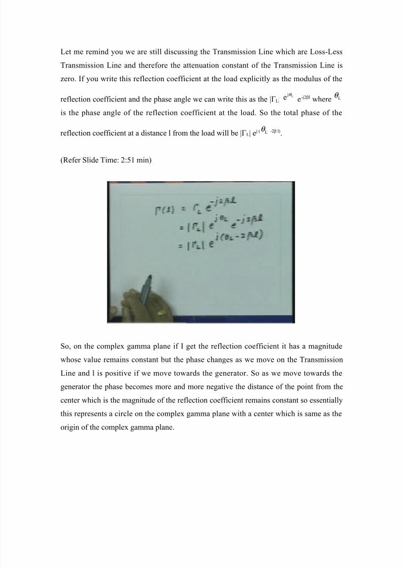
Let me remind you we are still discussing the Transmission Line which are Loss-Less

Transmission Line and therefore the attenuation constant of the Transmission Line is

ero. f you write this reflection coefficient at the load explicitly as the modulus of the

reflection coefficient and the phase angle we can write this as the /ΓL/L $

e

θ

e-$%&l where Lθ

is the phase angle of the reflection coefficient at the load. So the total phase of the

reflection coefficient at a distance l from the load will be /ΓL/ e $ ' Lθ -%& l.

'!efer Slide Time( %(*) min

So, on the complex gamma plane if get the reflection coefficient it has a magnitude

whose value remains constant but the phase changes as we move on the Transmission

Line and l is positive if we move towards the generator. So as we move towards the

generator the phase becomes more and more negative the distance of the point from the

center which is the magnitude of the reflection coefficient remains constant so essentially

this represents a circle on the complex gamma plane with a center which is same as the

origin of the complex gamma plane.



So can plot this on the complex gamma plane this is u, this is $v get a circle on the

complex gamma plane whose radius is /ΓL/ and the angle is ' Lθ -%& l.

'!efer Slide Time( 01(*+ min

So l is positive as we move towards the generator so this #uantity becomes more and

more negative so the point essentially moves on this circle in the cloc"wise direction. So

the movement of on Transmission Line by a distance l is e#ual to a rotation on this circle

in the cloc"wise direction.

2ow for this circle the magnitude of reflection coefficient is same no matter what point

you ta"e on this. So the phase angle changes for different points on Transmission Line

but the magnitude of reflection coefficient remains same. 3nd we "now that the SW!

on Transmission Line is

L

L

)

)-

+ Γ

Γ as we saw last time. So for this circle any point on this

circle this #uantity SW! is same because /ΓL/ is same for all the points on this circle and

that is the reason the SW! is same for all points on this circle. So you ta"e any

impedance which lies on this circle it magnitude of reflection coefficient will be same

and that is the reason the SW! will be same.



'!efer Slide Time( 0*(40 min

5onse#uently we call these circles as the constant SW! circles. 6ou have to draw these

circles whenever we solve the Transmission Line problems using smith chart. So smith

chart readily gives you the set of circles which are constant resistance and constant

reactance circles and while solving the problem we have to draw the circles called the

constant SW! circles on the smith chart and then do the transmission line calculations.

3s we can see there are special properties for the constant SW! circles, firstly the

center of all constant SW! circle is same as the origin of the complex gamma plane,

secondly for all passive loads the magnitude of reflection coefficient is always less than

or e#ual to one so these circles are concentric circles with origin as the center of the

circles and the maximum radius for this circle is one. Larger the radius gives you more

reflection coefficient that means worse is the impedance match so what that tells you now

is if you ta"e a point which is closer to the origin of the reflection coefficient plane it

denotes smaller magnitude of reflection coefficient which means smaller reflection which

again means better magnitude.



So visually whenever we have impedance mar"ed on the smith chart or on the complex

gamma plane visually if the point is closer towards the center of the smith chart better is

the match because that is representing smaller value of the magnitude of the reflection

coefficient. With this understanding and superposing the constant SW! circle on the

smith chart then we can solve the Transmission Line problems.

7owever as mentioned last time you may re#uire many times the connections of

Transmission Lines which could be in the form of parallel connections and we "now

from electrical circuit analysis that whenever we have parallel connections it is easier to

deal with the admittances rather than impedances. Till now, we have been tal"ing about

the load impedances or any impedance on Transmission Line however now if you want to

ma"e parallel connections we have to represent this loads and other characteristic in

terms of admittances.

So what we first do before we go into analysis of Transmission Line using smith chart let

us find out how the smith chart would loo" li"e if do all the calculations in terms of the

admittances. Since the smith chart deals with the normalied impedances as we have seen

the same thing we can do for the admittances. So we can first define the normalied

admittances on Transmission Line and for that we will re#uire the characteristic

admittance of Transmission Line.

So what you do first is we define a #uantity called the characteristic admittance which is

denoted by 60 and that is nothing but one upon the characteristic impedance 80.



'!efer Slide Time( 0+()* min

Then every admittance which we see on Transmission Line is normalied with respect to

the characteristic admittance of the Transmission Line. So following the same notation as

we did for the impedances normalie the admittance which is denoted by y bar that will

be e#ual to the actual admittance divided by characteristic admittance on the

Transmission Line. Similarly the load admittance normalied will be e#ual to the actual

load admittance divided by the characteristic admittance of the Transmission Line.



'!efer Slide Time( 0+(** min

9nce we ma"e this definition for the characteristic admittance and the admittances on the

Transmission Line then one can as" how do write down the reflection coefficient in

terms of the admittances. :oing from the definition of the reflection coefficient which we

have derived in terms of the impedance the Γ at any location is

0

0

8 8

8 ; 8

−

.

The admittance will be

)

8 the characteristic admittance will be 0

)

8 so you can write this

as

0

0

) )6 6

) )6 6

−

+

which will be e#ual to

0

0

6 6

6 ;6

−

.



'!efer Slide Time( ))(0+ min

f want to write in terms of normalied admittances can ta"e 60 common so that will

be e#ual to

) 6

);6

−

.

f ta"e negative sign common this will be

( )6 )

6;)− −

so we can write this as

6 )

6;)−

and

the minus sign is nothing but the phase change of )<0=. So this is same as e $>.



'!efer Slide Time( ))(4+ min

So a reflection coefficient if write it in terms of normalied admittances it is same as if

got the reflection coefficient by using normalied impedance except there is going to be a

phase change of >.

What that means is if ta"e the same normalied value of impedance and admittance and

calculate what that reflection coefficient would be the magnitude of the reflection

coefficient would be same but the phase difference between the reflection coefficients

will be )<0= or in other words on complex gamma plane the )<0= phase change would

correspond to a rotation by an angle )<0=. So essentially the normalied admittances and

normalied impedances can be dealt in a same way except whenever we are doing

calculation for the normalied impedance there is a rotation of )<0= on the complex

gamma plane otherwise all other things remain same. So what essentially we are saying is

if ta"e the gamma plane as we did it earlier here and ta"e certain value of the

normalied impedance get the reflection coefficient here if ta"e the same normalied

value for the admittance the point has to rotate by )<0= so if ta"e a diagonally opposite

point on this circle that is the point which will correspond to the complex reflection

coefficient for the normalied admittance.



So essentially as far as the set of circles are concerned called the smith chart if rotate

every point on the smith chart by one eighty degrees get the set of circles for the

normalied admittances.

Let us say the normalied admittance is denoted by g ; $b so y is the normalied

admittance and let us denote that by the conductance g plus the susceptance $b which is

same as the actual conductance plus the actual susceptance divided by the characteristic

admittance y0.

'!efer Slide Time( )4(1? min

So if have a admittance on line which is given by the conductance g plus susceptance b

and normalied characteristic admittance y0 can calculate the normalied admittance on

the transmission line which is g ; $b.

So if interchange r with g and x with b will get set of circle which will be constant g

circle for constant conductance circles and constant susceptance circles and these circles

will be rotated version on the complex gamma plane by )<0=. What that means is if



have initially a chart there is rotation of every point on this around the center of the smith

chart which is origin of the complex gamma plane by )<0=.

'!efer Slide Time( )*(4@

So if "eep gamma plane fixed that this is the real axis of the gamma plane, this is the

imaginary axis of the gamma plane then every point on this will rotate and the constant

conductance and the constant susceptance will loo" li"e that. 2ow in this case these

circles which were earlier constant resistance circles are now the constant conductance

circles these circles which were constant reactance circles are now constant susceptance

circles so nothing is changed as far as the smith chart is concerned except the first smith

chart is rotated by )<0=.

2ow there are two things if "eep the axis for the complex reflection coefficient same

then the smith chart will be rotated by )<0= alternatively can "eep smith chart same and

rotate the complex gamma plane axis by )<0= whenever do the calculation for the

admittances. So if develop an understanding that will not rotate the smith chart will

use always in this form which means the most clustered portion of the smith chart is on

my right then if do the impedance calculations the positive real axis is towards right and



the positive imaginary axis is upwards, however if do the calculation by using this chart

for admittances then the real axis will be on my left and the imaginary axis will be

downwards. 2ormally whenever we do the smith chart calculations we do not rotate the

smith chart. We follow this convention that the smith chart is fixed but for the impedance

the gamma axis is li"e that where as when i go to admittances i get the gamma axis which

will be li"e this.

So depending upon whether we are doing any calculation for the impedances or the

admittances and if re#uire the phase measurement phase angle measurement in the

complex gamma plane then appropriately the axis has to be rotated by )<0= depending

upon whether am using the impedance or am using the admittance.

Aut if do not want to find out the phase of the reflection coefficient then the axis of

gamma plane does not come into picture it is $ust the impedances and admittances which

we want to use on the smith chart. So we can use the smith chart for the admittance as

well as for the impedance calculations without worrying of the complex gamma plane

axis. That is the reason why if you loo" at the smith chart carefully you will see that the

upper half of the smith chart is denoted by ';x, ;b, lower is denoted by 'Bx, -b, the

circles are denoted by either r or g. So any normalied value of r which is e#ual to the

same normalied value g will represent the same circle.

So as long as we are dealing with the normalied #uantities the impedance and

admittance can be treated exactly same way on the smith chart. 7owever the normalied

values of g and r or b and x have different meaning physically, they do not represent same

physical conditions. Cor example suppose consider r D 0, x D0 which corresponds to the

short circuit conditions the impedances is ero at that point but if ta"e a normalied

value g D 0, b D 0 which represents the admittance e#ual to ero is not short circuit that is

the open circuit condition on the line.

So the normalied values of impedances admittances can be treated exactly same way but

when we go for the physical conditions the physical conditions are not same for the same



normalied value of the impedance and admittance. So as we loo"ed at the point last time

which was some special points on the smith chart, now let us loo" at these points for the

admittance smith chart.

f ta"e the smith chart and say suppose these values are not impedances but they are

admittances that means if replace r by g and x by b this point represent g D 0, b D 0

which is open circuit, this points represents g D E, b D E which is short circuit, the upper

half which is the positive value of susceptance represent capacitive loads and the negative

value of susceptance represent the inductive load.

'!efer Slide Time( %0()@ min

So if "eep the smith chart fixed then while doing calculation with the admittances the

upper half of the smith chart represents the capacitive load, the lower half represent the

inductive load this is open circuit point and this is short circuit point. Since the resistance

circles are symmetric there is no difference so replacing r by g essentially tells you the g

value is increasing from ero to infinity as we move on this side but the point is going

from the open circuit to the short circuit. Then "eeping these things in mind the use of

smith chart for impedance and admittance calculation is very straight forward.



the characteristic admittances. So let us say my impedance was 8L so first step which do

is normalie it get

L

0

8

8 which is 8 .

'!efer Slide Time( %1(1@ min

2ow read on the smith chart this point, recall the smith chart as set of circles, this is the

constant resistance circles which are going li"e that or constant reactance circle which go

li"e that. Let us say this is given by some r ; $x li"e that. Cirst identify a constant

resistance circle which is having this value r, let us say that circle is this side for which

the resistance value is this value r. Then identify a circle for which the reactance value is

this x which is will be this value the intersection of these two circles the constant resistant

circle which is having value r and a constant reactance circle which is having value x.

2ow this point represents this normalied impedance 8 so this point here is 8 .

9nce this point is mar"ed on the smith chart then calculation of reflection coefficient is

very straight forward because now the point has been mar"ed on the complex gamma

plane so if read of this value on complex gamma plane that directly gives you the



complex reflection coefficient so if measure the distance from the smith chart this is my

origin and let me draw now the complex gamma axis which is not drawn on the smith

chart so this is my u axis this is my $v axis and this is the origin. f measure the distance

of this point that gives me the magnitude of the reflection coefficient Γ L and the angle

that means generally we measure the angle on the complex plane from the real axis this

angle is the angle of the complex reflection coefficient at the load end. So this angle is

nothing but GL and this distance is /ΓL/.

'!efer Slide Time( %?(%+ min

So first thing on standard smith chart you find out the radius of this by using any scale

then measure this distance the maximum distance of the smith chart is unity so any

distance which you get on the smith chart normalied with respect to the maximum

distance that #uantity directly will give you the magnitude of the reflection coefficient

and the angle which this radius vector ma"es with the right hand horiontal axis is the

real gamma axis that is the angle of the reflection coefficient at the load end.

So without doing any calculations $ust by measuring this distance and this angle can get

the reflection coefficient from the complex impedance. Hxactly same thing can do for



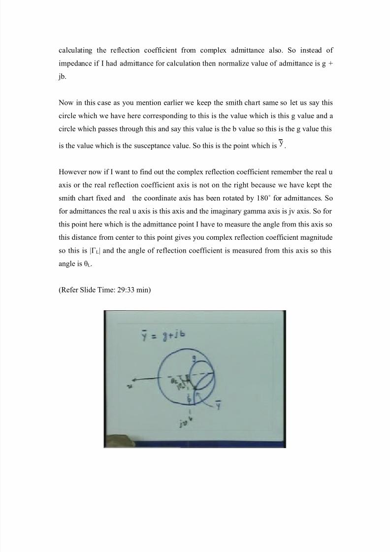
calculating the reflection coefficient from complex admittance also. So instead of

impedance if had admittance for calculation then normalie value of admittance is g ;

$b.

2ow in this case as you mention earlier we "eep the smith chart same so let us say this

circle which we have here corresponding to this is the value which is this g value and a

circle which passes through this and say this value is the b value so this is the g value this

is the value which is the susceptance value. So this is the point which is y .

7owever now if want to find out the complex reflection coefficient remember the real u

axis or the real reflection coefficient axis is not on the right because we have "ept the

smith chart fixed and the coordinate axis has been rotated by )<0= for admittances. So

for admittances the real u axis is this axis and the imaginary gamma axis is $v axis. So for

this point here which is the admittance point have to measure the angle from this axis so

this distance from center to this point gives you complex reflection coefficient magnitude

so this is /ΓL/ and the angle of reflection coefficient is measured from this axis so this

angle is GL.

'!efer Slide Time( %+(11 min



So "eeping in mid whether we are using normalied impedances or normalied

admittances appropriate rotation of the coordinate axis has to be made on the smith chart.

Aut once you do that then the calculation of the complex reflection coefficient is very

straight forward mar" the normalied point on the smith chart, find out the radial distance

from the center of the smith chart to that mar"ed point which gives you the magnitude of

the reflection coefficient, measure the angle from the real axis of the reflection coefficient

for the radius vector and that gives you the angle of the complex reflection coefficient.

9ne can have exactly opposite problems many times somebody might give you a

reflection coefficient then you have to find out what is the corresponding load. So the

problem is very straight forward, mar" the point on the complex reflection coefficient the

magnitude is given to you, the angle is given so you can draw this point. 9nce you get

this point read out the circles which are passing through these points so essentially you

read out the coordinates on this constant resistance and constant reactance circle and that

give you the corresponding value of the impedance. So without doing any analytic

calculation $ust by graphical measurements of angle and distance you can find out the

reflection coefficient from the impedance or admittance and vice versa.

2ow, one can go to the next stage that if the load impedance is given to you then you

would li"e to find out the reflection coefficient or impedance at some other location on

the Transmission Line. So the problem is given, say 8L is normalied or yl and you want

to find out ICind at a distance l from the loadJ

:o to the smith chart generally we draw only these three circles where r e#ual to one

circle, r e#ual to ero circle then the reactance circles which are two circles li"e that so

this corresponds to x D ;), x D -), r D ), r D 0 and x D0 so normally $ust for clarity we $ust

draw only this few circles to represent a smith chart.



'!efer Slide Time( 1%(1@ min

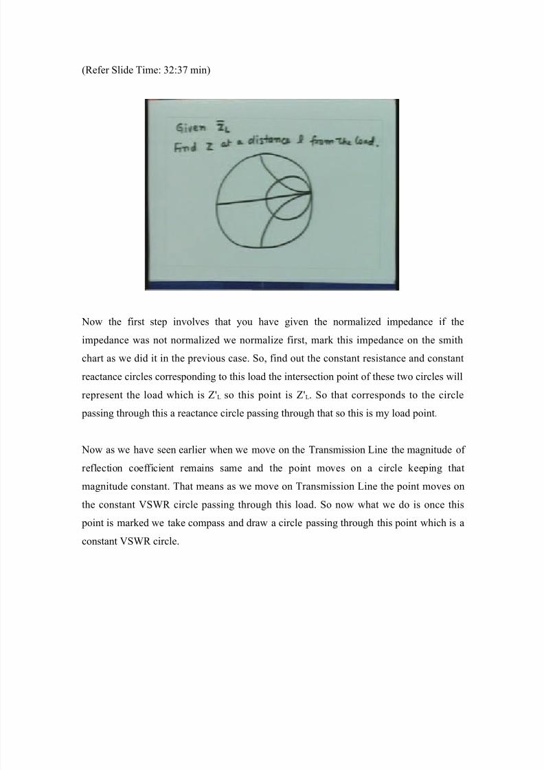
2ow the first step involves that you have given the normalied impedance if the

impedance was not normalied we normalie first, mar" this impedance on the smith

chart as we did it in the previous case. So, find out the constant resistance and constant

reactance circles corresponding to this load the intersection point of these two circles will

represent the load which is 8KL so this point is 8KL. So that corresponds to the circle

passing through this a reactance circle passing through that so this is my load point.

2ow as we have seen earlier when we move on the Transmission Line the magnitude of

reflection coefficient remains same and the point moves on a circle "eeping that

magnitude constant. That means as we move on Transmission Line the point moves on

the constant SW! circle passing through this load. So now what we do is once this

point is mar"ed we ta"e compass and draw a circle passing through this point which is a

constant SW! circle.



'!efer Slide Time( 11(** min

2ow as we move on Transmission Line the angle changes by %&l in the cloc"wise

direction, normally for the standard smith chart the distance is directly mar"ed on the

periphery of the smith chart instead of mar"ing the angles on the periphery. how do we

do is a distance of %&l if ta"e one rotation on the smith chart the angle change will be

e#ual to %>, if move on the smith chart by %> that is e#ual to %&l

%%. .lπ λ



'!efer Slide Time( 14(4* min

So l will be e#ual to %

λ

. That means one full rotation on the smith chart or the constant

SW! circle corresponds to a distance of %

λ

that means if move by a distance of %

λ

on

the constant SW! circle reach to the same point.

3nd that ma"es sense because if you recall the characteristic of Transmission Line we

had seen that the impedance characteristic of Transmission Line repeat itself for every

distance of %

λ

. That is what essentially we are reaffirming saying that by ta"ing one

rotation on the constant SW! circle we reach to the same point and beyond that again

the characteristics are repeated. So the angles here which are the load angle minus %&l

now can be calibrated directly in terms of the wavelength. So generally we have the outer

circle of the smith chart mar"ed with the wavelength and with the calibration that the full

one rotation on the smith chart is e#ual to %

λ

. So the distance from this point to this point



is 4

λ

from, this point to this point is 4

λ

. 9nce we get that then want to find the

impedance at a distance l which is this impedance.

So now you move from the load impedance by a distance l or rotate this point in the

cloc"wise direction by an angle which is e#ual to %&l. Let us say this was the initial angle

which was there, rotate now my point on the constant SW! circle by an angle which

is %&l.

'!efer Slide Time( 1?(*? min

eep in mind we are rotating in the cloc"wise direction because we are moving from the

load towards the generator and distances measured towards the generator are positive

distances that means the l is positive. Therefore the angle becomes more negative so the

point moves in a cloc"wise direction. This sense of rotation is very important in doing all

Transmission Line calculations.

So if move in the cloc"wise direction by a distance of %&l would reach to a location l

on the Transmission Line. Then this point would correspond to the reflection coefficient



at a distance l from the load. The magnitude of reflection coefficient remains same which

is same as this so this angle was theta l, this angle will be the angle of the reflection

coefficient at location l can read this angle the magnitude is same is what had got from

here. So got the complex reflection coefficient at location l. So this is my Transmission

Line, this is my load impedance 8L the reflection coefficient here was ΓL if move a

distance l over here the reflection coefficient at this then Γ is represented by this point.

'!efer Slide Time( 1<(1* min

9nce get the reflection coefficient li"e this can $ust find out what are the constant

resistance and constant reactance circle are passing through this point and can read of

that value. So can get the impedance corresponding to this point which is nothing but

the transform impedance at a distance l from the load. This point represents Γ at a

distance l and if read of the value at the impedance that will be the impedance at that

point at a distance l so here this is the impedance which is at this point.

3nalytically if you remember the impedance transformation re#uires calculation of the

cosine sine functions and the expression is rather complicated. With the help of smith

chart the impedance transformation is very simple you simply draw this SW! circle



passing through the load point move by an angle which is e#ual to %&l read of the value

of this new point which you have got here that gives you the transform impedance at a

distance l.

So the calculation of impedance and reflection coefficient at any other location on the

Transmission Line is extremely simple and straight forward by using the smith chart.

2ow in this case we were transforming the impedance which was load impedance to a

location l towards the generator. 9ne may have a general situation that a impedance is

given at any arbitrary location on Transmission Line and you would li"e to find the

transformed impedance at some other location on the line. 7ow does the procedure

changesF The procedure is exactly same wherever you "now the impedance first mar" the

impedance, draw the constant SW! circle passing through this point move by an angle

%&l either cloc" wise direction or anti cloc" wise direction depending upon whether am

moving towards generator or away from the generator find the new point read out the

value that will give you the transformed impedance at the new location.

So in general case either might move in the cloc"wise direction or might move in the

anti cloc"wise direction and that will depend upon whether am moving towards the

generator or away from the generator. So let me again mention that the sense of rotation

in impedance transformation calculation is extremely important because that tells you

whether you are moving towards the generator or away from the generator. So in all

Transmission Line calculations you should always remember that which direction the

generator is because that will decide the movement on the Transmission Line and that

will decide which way you should rotate on the constant SW! circle on the smith chart.

2ow if replace the impedances by the admittances if am not interested in the

calculations of the reflection coefficient as am interested only in the transformed

admittances then the axis for reflection coefficient do not come into picture. So the

procedure for transforming the impedance and the admittance are exactly identical. What

you do is $ust simply ta"e this point as a normalied admittance point, mar" the



normalied admittance 8 draw this circle which is constant SW! circle, rotate it by an

angle which is e#ual to %&l read this point so that this point will correspond to the

admittance at that location and that value can be straight away read out from this smith

chart.

So the transformation of impedance or admittance is exactly identical on the smith chart.

3s we saw earlier if have to find out the phase of the reflection coefficient then only

mar"ing of reflection coefficient axis comes into picture and then you have to remember

that the real axis is rightwards for the impedances where as the real axis is leftwards for

the admittances. Aut otherwise for impedance transformation calculation once the

impedance and admittance is normalied the procedure for the transformation is exactly

identical.

2ext thing then one can as" is that have the load impedance which is connected to the

line the parameter which is of interest is one is magnitude of reflection coefficient which

gave you the reflection but we have define a another #uantity which is the measure of

reflection and that is the SW! so one way of finding SW! is you get the

measurement of reflection coefficient, magnitude of reflection coefficient from the

constant SW! circle then use the formula

L

L

)

) -

+ Γ

Γ and you will get the reflection

coefficient.

7owever once you have smith chart with you then you do not have to do even this

calculation you can $ust read of the value on the smith chart. So let us say this is my smith

chart and let us say have some impedance which is mar"ed here this is my some load

impedance 8L.



'!efer Slide Time( 44(%0 min

3s routine we draw the constant SW! circle passing through this so we get a circle

which is this as move on the Transmission Line move on this circle. 2ow recall the

SW! is nothing but ratio of the maximum impedance seen on the line divide by the

characteristic impedance we have derived it earlier so we have ! max which we see on the

line which is e#ual to 80 into the SW! or in terms of normalied #uantity if ta"e ! max

normalie that is ! max divide by 80 that is nothing but is e#ual to M. So, the maximum

value of the resistance in terms of normalied #uantity is nothing but the SW!. 2ow as

we move on this circle here the highest value of resistance will be seen when this circle

intersect this line.

The right most point on this circle corresponds to an impedance which is ! max normalied

and the reactance for that is ero so this point here the right most point on this axis that

corresponds to normalied ! max and normalied ! max is nothing but M. So if read out the

value of this point from the smith chart they straight away gives you the SW! so this

#uantity straight away gives me the value of M.



Similarly as we "now the minimum value which we see on Transmission Line is

08

ρ so

we have seen earlier ! min D

08

ρ .

So again normalied ! min will be

)

ρ so on this circle the minimum resistance which see

is corresponds to this point so if read of this value will directly give me

)

ρ .

'!efer Slide Time( 4@()0 min

So again once the load impedance or any impedance is mar"ed on the smith chart and this

circle which is called the constant SW! circle is drawn on the smith chart. Then

calculation of SW! reflection coefficient transformation impedance all is very straight

forward problem it is $ust a matter of reading of the values from different locations on the

smith chart. So this is the way you can calculate SW! using smith chart.



'!efer Slide Time( 4@(*< min

2ext thing one can do is find out the location of the voltage or the current maximum or

minimum on the Transmission Line and then one can use the information to find out that

$ust loo"ing at the standing wave pattern on Transmission Line what "ind of load that

Transmission Line is terminated line.

So ta"ing a simple case let us say some load impedance mar"ed the load impedance at the

smith chart then you want to find out what is the distance of the voltage maximum or

current maximum or voltage minimum or current minimum from the load end of the

Transmission Line.

What we want to do now as we did earlier is we want to find out find distance of voltage

or current maximum on the line. Let us do the same thing we ta"e the smith chart mar"

the load impedance on the line lets say the load impedance is here this is nothing but your

8L normalie. 3gain as a first step draw the constant SW! circle passing through this

point get this point.



2ow if you go bac" to your basic understanding of Transmission Line we "now that at

the voltage maximum as the current is minimum so at that location the impedance seen is

the maximum impedance which is nothing but ! max and wherever you have voltage

minimum at that location current is maximum and impedance seen will be ! min. That

means the extreme point which is this point corresponds to an impedance which is ! max

that means this corresponds to a location on Transmission Line where voltage is

maximum or current is minimum. So this point here now corresponds to the voltage

maximum or current minimum location. Similarly this point here which represents the

current minimum resistance on the line corresponds to voltage minimum or current

maximum location.

'!efer Slide Time( *)(11 min

We want to find out this location from the load. The $ob is very simple you draw a radius

vector passing through the load its here, if move towards the generator up to this point

on the constant SW! circle will reach to the location where the resistance is maximum

or the voltage is maximum. So essentially we can find out what is this angle this arc here

is. Whatever angle get divide it by %& then will get a distance of the voltage

maximum from the load point. can use our understanding that the voltage minima and



voltage maxima are separated by distance of 4

λ

so can add a distance of 4

λ

to find out

the location of voltage minimum once "now this distance or can measure this angle all

the way up to this divide by %& to find out the location of the voltage maximum.

So if this angle was Gmax then the location of voltage maximum lmax will be e#ual to the

max

%

θ

β . So finding the location of voltage maximum or current minimum is extremely

straight forward.

'!efer Slide Time( *1()@ min

9nce you mar" the impedance on this draw the constant SW! circle $ust find out the

angle from this radius vector up to this horiontal line on right hand side and you would

get this angle which if you divide by %& you will get a distance of voltage maximum.

We will continue with this and then in next lecture we will view this information to find

out what is the impedance $ust by loo"ing at the standing wave patterns on the

Transmission Line. Than" you.

Transmission Lines and E.M. Waves lec 08.docx

Documents

Transcript of Transmission Lines and E.M. Waves lec 08.docx