Translating B to TLA+ for Validation with TLC:There and Back Again

(Technical Report)

Dominik Hansen and Michael Leuschel

Institut fur Informatik, Universitat Dusseldorf??

Universitatsstr. 1, D-40225 Dusseldorfdominik.hansen@uni-duesseldorf.de, leuschel@cs.uni-duesseldorf.de

Abstract. The state-based formal methods B and TLA+ share the com-mon base of predicate logic, arithmetic and set theory. However, there arestill considerable differences, such as the way to specify state transitions,the different approaches to typing, and the available tool support. In thispaper, we present a translation from B to TLA+ to validate B specifica-tions using the model checker TLC. We provide translation rules for almostall constructs of B, in particular for those which are missing in TLA+. Thetranslation also includes many adaptions and optimizations to allow efficientchecking by TLC. Moreover, we present a way to validate liveness propertiesfor B specifications under fairness conditions. Our implemented translator,Tlc4B, automatically translates a B specification to TLA+, invokes themodel checker TLC, and translates the results back to B. We use ProB todouble check the counter examples produced by TLC and replay them inthe ProB animator. We also present a series of case studies and benchmarktests comparing Tlc4B and ProB.Keywords: TLA+, B-Method, Tool Support, Model Checking, Animation.

1 Introduction and Motivation

B [1] and TLA+ [8] are both state-based formal methods rooted in predicate logic,combined with arithmetic, set theory and support for mathematical functions. How-ever, as already pointed out in [5], there are considerable differences:

– B is strongly typed, while TLA+ is untyped. For the translation it is obviouslyeasier to translate from a typed to an untyped language than vice versa.

– The concepts of modularization are quite different.– Functions in TLA+ are total, while B supports relations, partial functions,

injections, bijections, etc.– TLA+ has several constructs which are absent in B, such as an if/then/else

for expressions and predicates1 or the choose operator.

?? Part of this research has been sponsored by the EU funded FP7 projects 214158 (DE-PLOY) and 287563 (ADVANCE).

1 B only provides an if/then/else for substitutions.

– B is limited to invariance properties, while TLA+ also allows the specificationof liveness properties.

As far as tool support is concerned, TLA+ is supported by the explicit statemodel checker TLC [13] and more recently by the TLAPS prover [2]. TLC has beenused to validate a variety of distributed algorithms (e.g., [4]) and protocols. B hasextensive proof support, e.g., in the form of the commercial product AtelierB [3]and the animator, constraint solver and model checker ProB [9, 10]. Both AtelierBand ProB are being used by companies, mainly in the railway sector for safetycritical control software. In an earlier work [5] we have presented a translation fromTLA+ to B, which enabled applying the ProB tool to TLA+ specifications. Inthis paper we present a translation from B to TLA+, this time with the maingoal of applying the model checker TLC to B specifications. Indeed, TLC is avery efficient model checker for TLA+ with an efficient disk-based algorithm andsupport for fairness. ProB has an LTL model checker, but it does not supportfairness (yet) and is entirely RAM-based. The model checking core of ProB is lesstuned than TLA+. On the other hand, ProB incorporates a constraint solver andoffers several features which are absent from TLC, notably an interactive animatorwith various visualization options. Our approach is thus to replay the counter-examples produced by TLC within ProB to get access to those features and tovalidate the correctness of our translation. In this paper, we also present a thoroughempirical evaluation between TLC and ProB. The results show that for lower-level, more explicit formal models, TLC fares better, while for certain more high-level formal models the constraint solving capabilities of ProB lead to improvedperformance. The addition of a lower-level model checker thus opens up many newapplication possibilities.

2 Translation

The complete translation process from B to TLA+ and back to B is illustrated inFig. 1. Before explaining the individual phases, we will illustrate the translationwith an example and explain the various phases based on that example. Morespecific implementation details (e.g., about the parsing process) will be covered inSect. 4.

2.1 Example

Below we use a specification (adapted from [10]) of a process scheduler (Fig. 2). Thespecified system allows at most one active process at the same time. Each processcan qualify for being selected by the scheduler by entering a FIFO queue. Thespecification contains two variables: a partial function state mapping each processto its state (a process must be created before it has a state) and a FIFO queuemodeled as a (injective) sequence of processes. In the initial state no process iscreated and the queue is empty. Moreover, the specification has various operationsto create (new), delete (del), or add a process to queue (addToQueue). Additionally,

2

B Model SableCCB Parser

AbstractSyntaxTree

SemanticVerifier

(functionality inference,...)

TLCOptimizer

(subtype inference,...)

B-TLA+Translator

TLA +Model

TLCModel

Checker

CounterExample

TraceProB

Replay

TLC4BLibraries TLC4B

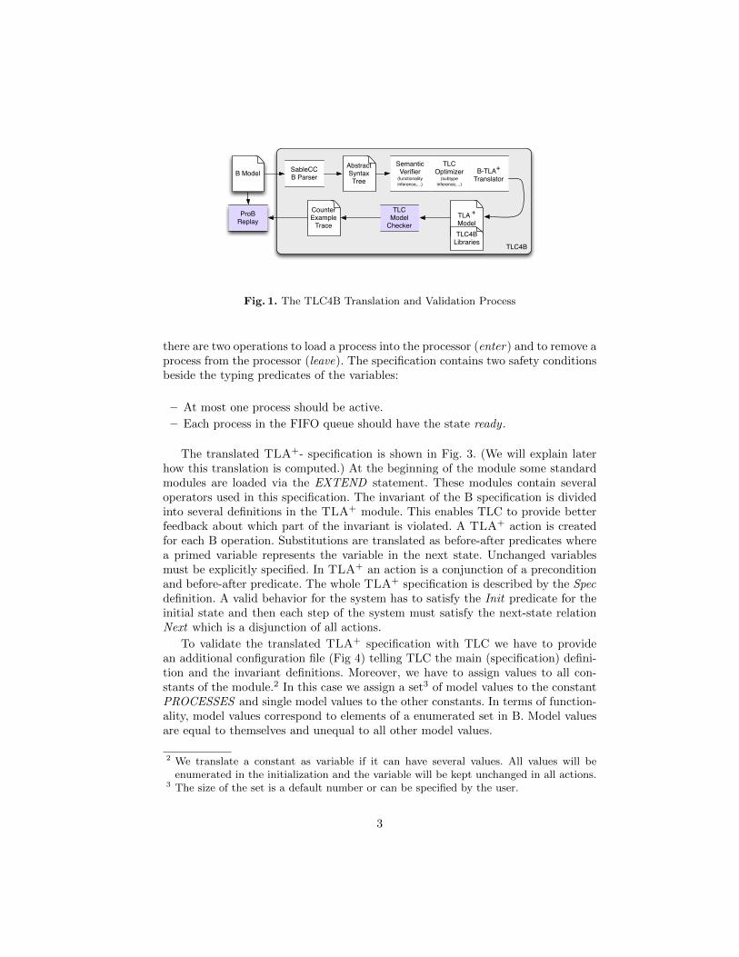
Fig. 1. The TLC4B Translation and Validation Process

there are two operations to load a process into the processor (enter) and to remove aprocess from the processor (leave). The specification contains two safety conditionsbeside the typing predicates of the variables:

– At most one process should be active.

– Each process in the FIFO queue should have the state ready .

The translated TLA+- specification is shown in Fig. 3. (We will explain laterhow this translation is computed.) At the beginning of the module some standardmodules are loaded via the EXTEND statement. These modules contain severaloperators used in this specification. The invariant of the B specification is dividedinto several definitions in the TLA+ module. This enables TLC to provide betterfeedback about which part of the invariant is violated. A TLA+ action is createdfor each B operation. Substitutions are translated as before-after predicates wherea primed variable represents the variable in the next state. Unchanged variablesmust be explicitly specified. In TLA+ an action is a conjunction of a preconditionand before-after predicate. The whole TLA+ specification is described by the Specdefinition. A valid behavior for the system has to satisfy the Init predicate for theinitial state and then each step of the system must satisfy the next-state relationNext which is a disjunction of all actions.

To validate the translated TLA+ specification with TLC we have to providean additional configuration file (Fig 4) telling TLC the main (specification) defini-tion and the invariant definitions. Moreover, we have to assign values to all con-stants of the module.2 In this case we assign a set3 of model values to the constantPROCESSES and single model values to the other constants. In terms of function-ality, model values correspond to elements of a enumerated set in B. Model valuesare equal to themselves and unequal to all other model values.

2 We translate a constant as variable if it can have several values. All values will beenumerated in the initialization and the variable will be kept unchanged in all actions.

3 The size of the set is a default number or can be specified by the user.

3

MODEL SchedulerSETS PROCESSES; STATE = {idle, ready, active}VARIABLES state, queueINVARIANT

state ∈ PROCESSES 7→ STATE& queue ∈ iseq(PROCESSES)& card(state−1[{active}]) ≤ 1& !x.(x ∈ ran(queue) ⇒ state(x) = ready)

INITIALISATION state := {} || queue := [ ]OPERATIONS

new(p) = PRE p /∈ dom(state)THEN state := state ∪ {(p 7→ idle)} END

del(p) = PRE p ∈ dom(state) ∧ state(p) = idleTHEN state := {p} �− state END

add(p) = PRE p ∈ dom(state) ∧ state(p) = idleTHEN state(p) := ready || queue := queue ← p END

enter = PRE queue 6= [ ] ∧ state−1[{active}] = {}THEN state(first(queue)) := active || queue := tail(queue) END

leave(p) = PRE p ∈ dom(state) ∧ state(p) = activeTHEN state(p) := idle END

END

Fig. 2. MODEL Scheduler

2.2 Translating Data Values and Functionality Inference

Due to the common base of B and TLA+, most data types exist in both languagese.g. sets, functions and numbers. As a consequence, the translation of these datatypes is almost simple.

A missing data type in TLA+ Relations are4, but TLA+ provides all necessarydata types to define relations based on the model of the B-Method. We representa relation in TLA+ as a set of tuples (e.g. {〈1,TRUE 〉, 〈1,FALSE 〉 〈2,TRUE 〉}).The drawback of this approach is that in contrast to B, TLA+’s own functionsand sequences are not based on the relations defined is this way. As an example,we cannot specify a function as a set of pairs in TLA+; in B it is usual to do thisas well as to apply set operators (e.g. the union operator as in r ∪ {2 7→ 3}) tofunctions or sequences. To support such a functionality in TLA+, functions andsequences should be translated as relations if they are used in a “relational way”. Itwould be possible to always translate functions and sequences as relations. But incontrast to relations, functions and sequences are built-in data types in TLA+ andtheir evaluation is optimized by TLC (e.g. lazy evaluation). Hence we extended theB type-system to distinguish between functions and relations. Thus we are able totranslate all kinds of relations and to deliver an optimized translation.

4 Relations are not mentioned in the language description of [8]. In [7] Lamport introducesrelations in TLA+ only to define the transitive closure.

4

module Schedulerextends Sequences, Relations, Functions, FunctionsAsRelations, SequencesExtendedconstants PROCESSES , idle, ready , activevariables state, queueSTATES

∆= {idle, ready , active}

Invariant1∆= state ∈ RelParFuncEleOf (PROCESSES , STATES)

Invariant2∆= queue ∈ ISeqEleOf (PROCESSES)

Invariant3∆= Cardinality(RelImage(RelInverse(state), {})) ≤ 1

Invariant4∆= ∀ x ∈ Range(queue) : RelCall(state, x ) = ready

Init∆= state = {} ∧ queue = 〈〉

new(p)∆= p /∈ RelDomain(state)∧ state ′ = state ∪ {〈p, idle〉} ∧ unchanged 〈queue〉

del(p)∆= RelCall(state, p) = idle∧ state ′ = RelDomSub({p}, state) ∧ unchanged 〈queue〉

addToQueue(p)∆= RelCall(state, p) = idle

∧ state ′ = RelOverride(state, {〈p, ready〉})∧ queue ′ = Append(queue, p)

enter∆= (queue 6= 〈〉 ∧ RelImage(RelInverse(state), {active}) = {})∧ state ′ = RelOverride(state, {〈Head(queue), active〉})∧ queue ′ = Tail(queue)

leave(p)∆= RelCall(state, p) = active∧ state ′ = RelOverride(state, {〈p, idle〉}) ∧ unchanged 〈queue〉

Next∆= ∨ ∃ p ∈ PROCESSES : new(p)∨ ∃ p ∈ RelDomain(state) : del(p)∨ ∃ p ∈ RelDomain(state) : addToQueue(p)∨ enter∨ ∃ p ∈ RelDomain(state) : leave(p)

vars∆= 〈state, queue〉

Spec∆= Init ∧ 2[Next ]vars

Fig. 3. Module Scheduler

5

SPECIFICATION SpecINVARIANT Invariant1, Invariant2, Invariant3, Invariant4CONSTANTSPROCESSES = {PROCESSES1,PROCESSES2, PROCESSES3}idle = idleready = readyactive = active

Fig. 4. Configuration file for module Scheduler

We use a type inference algorithm adapted to the extend B type-system toget the required type information for the translation. Unifying a function typewith a relation type will result in a relation type (e.g. P(Z × Z) for both sides ofthe equation λx .(x ∈ 1..3|x + 1) = {(1, 1)}). However there are several relationaloperators keeping a function type if they are applied to operands with a functiontype (e.g. ran, first or tail). For these operators we have to deliver two translationrules (functional vs relational).5 Moreover the algorithm verifies the type correctnessof the B specification (i.e. only values of the same type can be compared with eachother).

2.3 Translating Operators

In TLA+ some common operators such as arithmetic operators are not built-inoperators. They are defined in separate modules called standard modules whichcan be included at the top of a specification.6 We reuse the concept of standardmodules to include the relevant B operators. Due to the lack of relations in TLA+

we have to provide a module containing all relational operators (Fig. 5).Moreover B provides a rich set of function types (they are not part of the B

type system) which are missing in TLA+. A function type is a combination ofpartial/total and injective/surjective/bijective. In TLA+ we only have total func-tions. We group all missing functional operators together in an additional module(Fig. 6).

Some operators exists in both languages but their definitions differs slightly.For example, the B-Method requires that the first operand for the modulo operatormust be a natural number. In TLA+ it can be also a negative number.

Operator B-Method TLA+

a modulo b a ∈ N ∧ b ∈ N1 a ∈ Z ∧ b ∈ N1

To verify B’s well-definedness condition for modulo we use TLC’s ability to checkassertions. The special operator Assert(P , out) throws a runtime exception with the

5 For various reasons we do not redefine TLA+ built-in operators e.g. set operators.6 TLC supports operators of the common standard modules Integers and Sequences in a

efficient way by overwriting them with Java methods.

6

module Relationsextends FiniteSets, Naturals, TLCRelation(X , Y )

∆= subset (X ×Y )

RelDomain(R)∆= {x [1] : x ∈ R}

RelRange(R)∆= {x [2] : x ∈ R}

RelInverse(R)∆= {〈x [2], x [1]〉 : x ∈ R}

RelDomRes(S , R)∆= {x ∈ R : x [1] ∈ S} Domain restriction

RelDomSub(S , R)∆= {x ∈ R : x [1] /∈ S} Domain subtraction

RelImage(R, S)∆= {y [2] : y ∈ {x ∈ R : x [1] ∈ S}}

RelOverride(R1, R2)∆= {x ∈ R : x [1] /∈ RelDomain(R2)} ∪ R2

RelComposition(R1, R2)∆= {〈u[1][1], u[2][2]〉 : u ∈

{x ∈ RelRanRes(R1, RelDomain(R2))× RelDomRes(RelRange(R1), R2) :x [1][2] = x [2][1]}}

...

Fig. 5. Module Relations

module Functionsextends FiniteSetsRange(f )

∆= {f [x ] : x ∈ domain f }

Image(f , S)∆= {f [x ] : x ∈ S}

TotalInjFunc(S , T )∆= {f ∈ [S → T ] :

Cardinality(domain f ) = Cardinality(Range(f ))}ParFunc(S , T )

∆= union {[x → T ] : x ∈ subset S}

ParInjFunc(S , T )∆= {f ∈ ParFunc(S , T ) :

Cardinality(domain f ) = Cardinality(Range(f ))}...

Fig. 6. Module Functions

error message out if the predicate P is false. Otherwise, Assert will be evaluatedto true. The B modulo operator can thus be expressed in TLA+ as follows:

Modulo(a, b) = IF Assert(a ≥ 0, ”ERROR”)THEN a % b ELSE 0

The else clause will never reached because a runtime exception is thrown.We also have to consider well-definedness conditions if we apply a function call

to a relation as happened in the example translation (Sect. 2.1):

RelCall(r , x )∆= if Cardinality(r) = Cardinality(RelDom(r)) ∧ x ∈ RelDom(r)

then (choose y ∈ r : y [1] = x )[2]else Assert(FALSE , “ERROR”)

In summary, we provide the following standard modules for our translation:

– Relations (Sect. A.8)

7

– Functions (Sect. A.6)– SequencesExtended (Sect. A.7)– FunctionsAsRelations (Sect. A.9)– SequencesAsRelations (Sect. A.10)– BBuiltins (Sect. A.4)

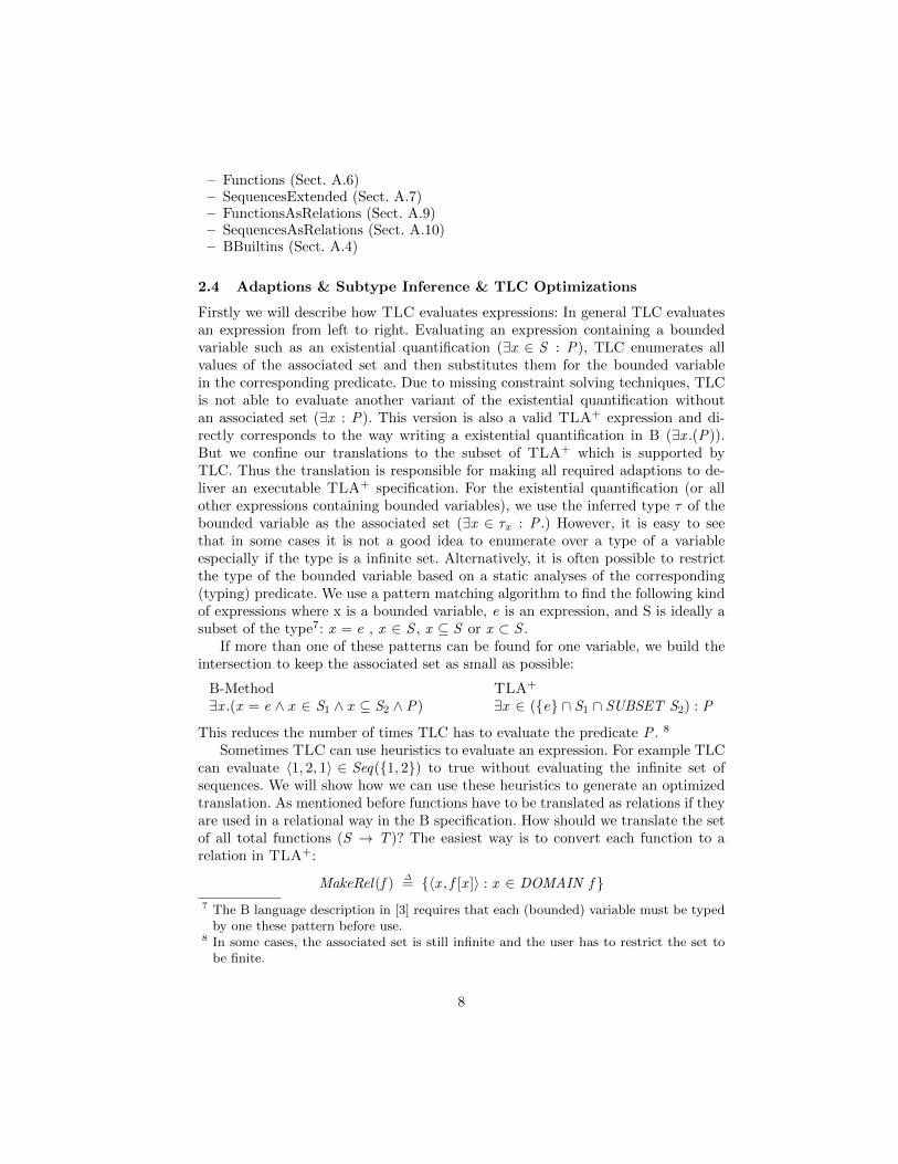
2.4 Adaptions & Subtype Inference & TLC Optimizations

Firstly we will describe how TLC evaluates expressions: In general TLC evaluatesan expression from left to right. Evaluating an expression containing a boundedvariable such as an existential quantification (∃x ∈ S : P), TLC enumerates allvalues of the associated set and then substitutes them for the bounded variablein the corresponding predicate. Due to missing constraint solving techniques, TLCis not able to evaluate another variant of the existential quantification withoutan associated set (∃x : P). This version is also a valid TLA+ expression and di-rectly corresponds to the way writing a existential quantification in B (∃x .(P)).But we confine our translations to the subset of TLA+ which is supported byTLC. Thus the translation is responsible for making all required adaptions to de-liver an executable TLA+ specification. For the existential quantification (or allother expressions containing bounded variables), we use the inferred type τ of thebounded variable as the associated set (∃x ∈ τx : P .) However, it is easy to seethat in some cases it is not a good idea to enumerate over a type of a variableespecially if the type is a infinite set. Alternatively, it is often possible to restrictthe type of the bounded variable based on a static analyses of the corresponding(typing) predicate. We use a pattern matching algorithm to find the following kindof expressions where x is a bounded variable, e is an expression, and S is ideally asubset of the type7: x = e , x ∈ S , x ⊆ S or x ⊂ S .

If more than one of these patterns can be found for one variable, we build theintersection to keep the associated set as small as possible:

B-Method TLA+

∃x .(x = e ∧ x ∈ S1 ∧ x ⊆ S2 ∧ P) ∃x ∈ ({e} ∩ S1 ∩ SUBSET S2) : P

This reduces the number of times TLC has to evaluate the predicate P . 8

Sometimes TLC can use heuristics to evaluate an expression. For example TLCcan evaluate 〈1, 2, 1〉 ∈ Seq({1, 2}) to true without evaluating the infinite set ofsequences. We will show how we can use these heuristics to generate an optimizedtranslation. As mentioned before functions have to be translated as relations if theyare used in a relational way in the B specification. How should we translate the setof all total functions (S → T )? The easiest way is to convert each function to arelation in TLA+:

MakeRel(f )∆= {〈x , f [x ]〉 : x ∈ DOMAIN f }

7 The B language description in [3] requires that each (bounded) variable must be typedby one these pattern before use.

8 In some cases, the associated set is still infinite and the user has to restrict the set tobe finite.

8

The resulting operator for the set of all total functions is:

RelTotalFunctions(S ,T )∆= {MakeRel(f ) : f ∈ [S → T ]}

However this definition has a disadvantage, if we just want to check if a singlefunction is in this set the whole set will be evaluated by TLC. Using the followingdefinition TLC avoids the evaluation of the whole set:

RelTotalFunctionsEleOf (S ,T )∆= {f ∈ SUBSET (S × T ) :

∧ Cardinality(RelDomain(f )) = Cardinality(f )∧ RelDomain(f ) = S}

In this case, TLC only checks if a function is a subset of the cartesian product (thewhole Cartesian product will not be evaluated) and the conditions are checked onlyonce. The advantage of the first definition is that it is faster to evaluate the wholeset. As a consequence, we use both definitions for our translation and choose the firstif TLC has to enumerate the set (e.g. ∃x ∈ RelTotalFunctions(S ,T ) : P) and thesecond testing if a function belongs to the set (e.g. f ∈ RelTotalFunctionsEleOf (S ,T )as an invariant).

3 Checking Temporal Formulas

One of the main advantages of TLA+ is that temporal properties can be specifieddirectly in the language itself. Moreover the model checker TLC can be used toverify such formulas. But before we show how to write temporal formulas for aB specification we first have to describe a main distinction between both formalmethods. In contrast to B, TLA+ allows stuttering steps at any time.9 This meansthat a regular step of a TLA+ specification is either a step satisfying one of theactions or an stuttering step leaving all variables unchanged. When checking aspecification for errors such as invariant violations it is not necessary to considerstuttering steps, because such an error will be detected in a state and stutteringsteps only allow self transitions and do not add additional states. For deadlockchecking stuttering steps are also not regarded by TLC, but verifying a temporalformula with TLC often ends in a counter-example caused by stuttering steps. Forexample, assuming we have a very simple specification of a counter in TLA+ witha single variable c

Spec = c = 1 ∧2[c′ = c + 1]c

We would expect that the counter will eventually reach 10 (3(c = 10)). HoweverTLC will report a counter-example, saying that at a certain state (before reaching10), a infinite number of stuttering will occur and 10 will never reached. Fromthe B site we do not want to care about these stuttering steps. TLA+ allowsthe adding of fairness conditions to the specification to avoid infinite stutteringsteps. Adding weak fairness for the next-state relation (WF (Next)) would prohibit

9 [Next ]vars ≡ Next ∨UNCHANGED vars

9

a infinite number of stuttering steps if a step of the next-state relation is possible(i.e. Next is always enabled):

WF (A) = ∨ 23(〈A〉vars)∨ 23(¬ENABLED(A))

However this fairness condition is too strong: It asserts that either the action Awill be executed infinitely often changing the state of the system (A must not be astuttering step)

〈A〉vars ≡ A ∧ vars ′ 6= vars

or A will be disabled infinitely often. Assuming weak fairness for the next staterelation will also eliminate user defined stuttering steps. User defined stutteringsteps result from B operations which do not change the state of the system (e.g.skip or call operations). These stuttering steps may cause valid counter-examplesand should not be eliminated. Hence, the translation should retain user definedstuttering steps in the translated TLA+ specfication and should disable stutteringsteps which are implicitly included. In [12] Richards describes a way to distinguishbetween these two kinds of stuttering steps in TLA+. We use his definition of “VeryWeak Fairness” applied to the next state relation (VWF (Next)) to disable implicitstuttering steps and allow user defined stuttering steps in the TLA+ specification:

VWF (A) = ∨ 23(〈A〉vars)∨ 23(¬ENABLED(A)∨ 23(ENABLED(A ∧UNCHANGED vars))

The definition of VWF is identical to WF except for an additional third case allow-ing infinite stuttering steps if A is a stuttering action (A∧UNCHANGED vars). 10

We define the resulting template of the translated TLA+ specification as follows:

Init ∧2[Next ]vars ∧VWF (Next)

We allow the B user to use following temporal operators to define liveness conditionsfor a B specification:

– 2f (Globally)– 3f (Finally)– ENABLED(op) (Check if the operation op is enabled)– ∃x .(P ∧ f ) (Existential quantification)– ∀x .(P ⇒ f ) (Universal quantification)– WF (op) (Weak Fairness will be translated to VWF)– SF (op) (Strong Fairness will be translated to “Almost Strong Fairness”11)– ¬, ∧, ∨, ⇒ (negation, conjunction, disjunction and implication)

10 However VWF(A) only says that infinite “unchanging” A steps are possible. It doesnot say that they will occur infinitely often. In TLA+ it is not possible to express that.

11 Analogical Richards defines “Almost Strong Fairness” (ASF) as a weaker version ofstrong fairness (SF) reflecting the different kinds of stuttering steps

10

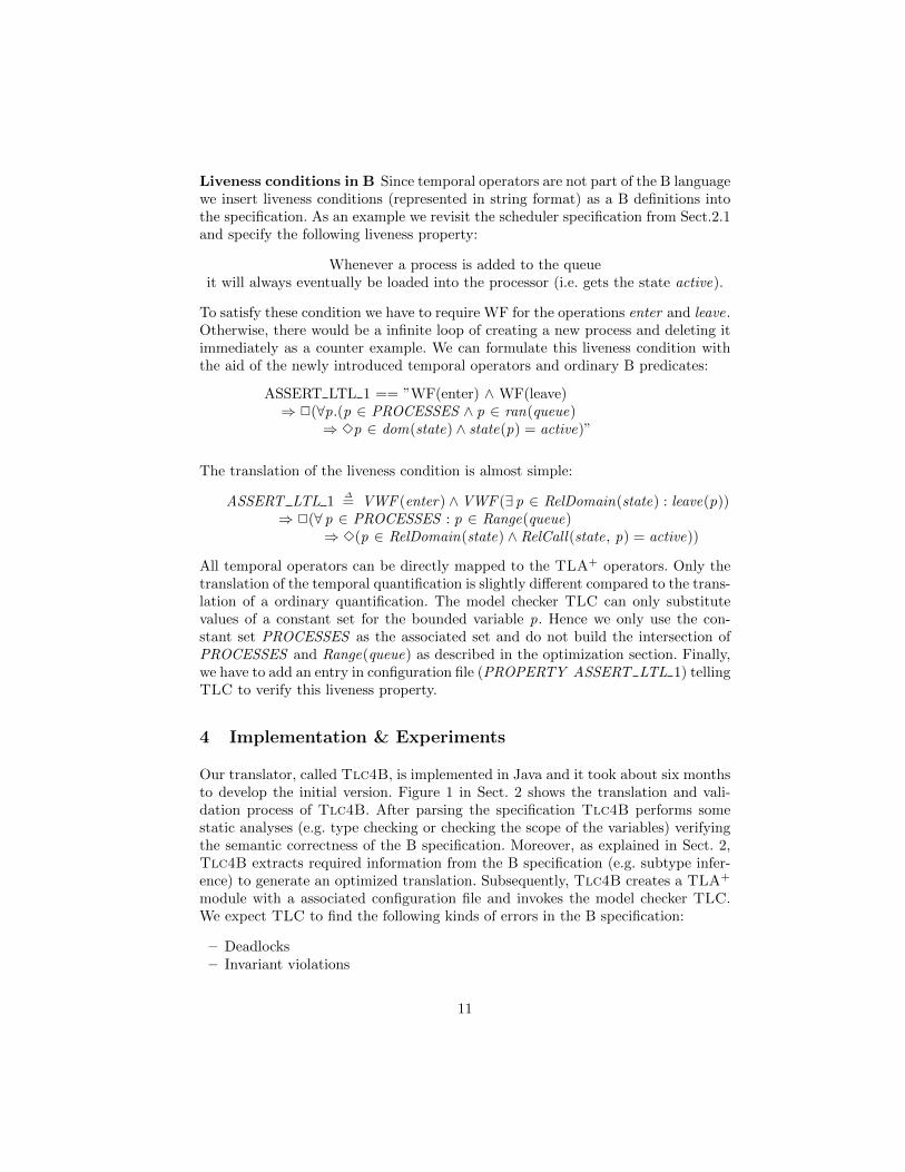
Liveness conditions in B Since temporal operators are not part of the B languagewe insert liveness conditions (represented in string format) as a B definitions intothe specification. As an example we revisit the scheduler specification from Sect.2.1and specify the following liveness property:

Whenever a process is added to the queueit will always eventually be loaded into the processor (i.e. gets the state active).

To satisfy these condition we have to require WF for the operations enter and leave.Otherwise, there would be a infinite loop of creating a new process and deleting itimmediately as a counter example. We can formulate this liveness condition withthe aid of the newly introduced temporal operators and ordinary B predicates:

ASSERT LTL 1 == ”WF(enter) ∧ WF(leave)⇒ 2(∀p.(p ∈ PROCESSES ∧ p ∈ ran(queue)

⇒ 3p ∈ dom(state) ∧ state(p) = active)”

The translation of the liveness condition is almost simple:

ASSERT LTL 1∆= VWF (enter) ∧VWF (∃ p ∈ RelDomain(state) : leave(p))

⇒ 2(∀ p ∈ PROCESSES : p ∈ Range(queue)⇒ 3(p ∈ RelDomain(state) ∧ RelCall(state, p) = active))

All temporal operators can be directly mapped to the TLA+ operators. Only thetranslation of the temporal quantification is slightly different compared to the trans-lation of a ordinary quantification. The model checker TLC can only substitutevalues of a constant set for the bounded variable p. Hence we only use the con-stant set PROCESSES as the associated set and do not build the intersection ofPROCESSES and Range(queue) as described in the optimization section. Finally,we have to add an entry in configuration file (PROPERTY ASSERT LTL 1) tellingTLC to verify this liveness property.

4 Implementation & Experiments

Our translator, called Tlc4B, is implemented in Java and it took about six monthsto develop the initial version. Figure 1 in Sect. 2 shows the translation and vali-dation process of Tlc4B. After parsing the specification Tlc4B performs somestatic analyses (e.g. type checking or checking the scope of the variables) verifyingthe semantic correctness of the B specification. Moreover, as explained in Sect. 2,Tlc4B extracts required information from the B specification (e.g. subtype infer-ence) to generate an optimized translation. Subsequently, Tlc4B creates a TLA+

module with a associated configuration file and invokes the model checker TLC.We expect TLC to find the following kinds of errors in the B specification:

– Deadlocks– Invariant violations

11

– Assertion errors– Goal found (a desired state is reached)– Properties violations (i.e., axioms over the B constants are false)– Well-definedness violations– Temporal formulas violations.

The results produced by TLC are translated back to B. For example, a goal predi-cate is translated as a negated invariant. If this invariant is violated, a “Goal found”message is reported. In some cases, TLC reports a trace leading to the state wherethe error (e.g. deadlock or invariant violation) occur. A trace is a sequence of stateswhere each state is a mapping from variables to values. Tlc4B translates the traceback to B. Tlc4B has been integrated into ProB as of version 1.3.7-beta: Theuser needs no knowledge of TLA+ because the translation is completely hidden.Counter-examples found by TLC are automatically replayed in the ProB anima-tor to give the user an optimal feedback. As shown in figure 7 counter-examplesfound by TLC are automatically replayed in the ProB animator (displayed in thehistory pane) to give the user an optimal feedback.

Fig. 7. ProB animator

The following examples show some fields of application of Tlc4B. The experi-ments were all run on a Macbook Air with Intel Core i5 1,8 GHz processor, running

12

TLC Version 2.05 and Prob version 1.3.7-beta9. The full details about the examplescan be found in the extended version of our paper [6].

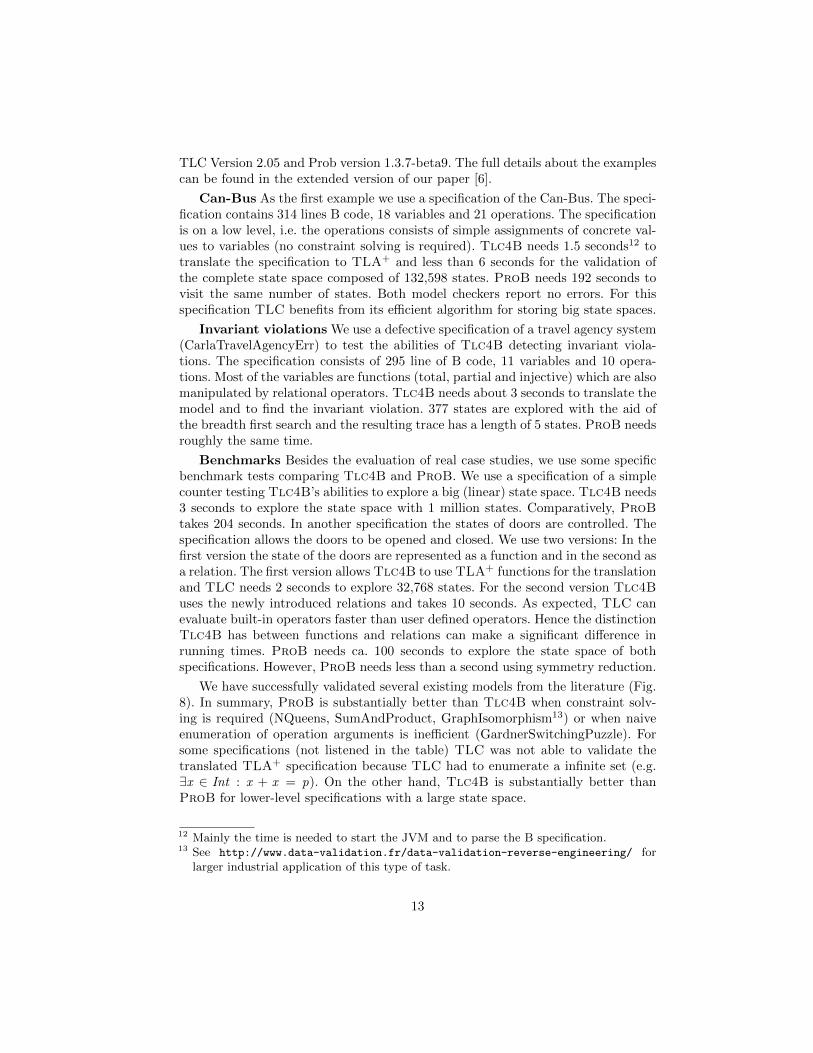
Can-Bus As the first example we use a specification of the Can-Bus. The speci-fication contains 314 lines B code, 18 variables and 21 operations. The specificationis on a low level, i.e. the operations consists of simple assignments of concrete val-ues to variables (no constraint solving is required). Tlc4B needs 1.5 seconds12 totranslate the specification to TLA+ and less than 6 seconds for the validation ofthe complete state space composed of 132,598 states. ProB needs 192 seconds tovisit the same number of states. Both model checkers report no errors. For thisspecification TLC benefits from its efficient algorithm for storing big state spaces.

Invariant violations We use a defective specification of a travel agency system(CarlaTravelAgencyErr) to test the abilities of Tlc4B detecting invariant viola-tions. The specification consists of 295 line of B code, 11 variables and 10 opera-tions. Most of the variables are functions (total, partial and injective) which are alsomanipulated by relational operators. Tlc4B needs about 3 seconds to translate themodel and to find the invariant violation. 377 states are explored with the aid ofthe breadth first search and the resulting trace has a length of 5 states. ProB needsroughly the same time.

Benchmarks Besides the evaluation of real case studies, we use some specificbenchmark tests comparing Tlc4B and ProB. We use a specification of a simplecounter testing Tlc4B’s abilities to explore a big (linear) state space. Tlc4B needs3 seconds to explore the state space with 1 million states. Comparatively, ProBtakes 204 seconds. In another specification the states of doors are controlled. Thespecification allows the doors to be opened and closed. We use two versions: In thefirst version the state of the doors are represented as a function and in the second asa relation. The first version allows Tlc4B to use TLA+ functions for the translationand TLC needs 2 seconds to explore 32,768 states. For the second version Tlc4Buses the newly introduced relations and takes 10 seconds. As expected, TLC canevaluate built-in operators faster than user defined operators. Hence the distinctionTlc4B has between functions and relations can make a significant difference inrunning times. ProB needs ca. 100 seconds to explore the state space of bothspecifications. However, ProB needs less than a second using symmetry reduction.

We have successfully validated several existing models from the literature (Fig.8). In summary, ProB is substantially better than Tlc4B when constraint solv-ing is required (NQueens, SumAndProduct, GraphIsomorphism13) or when naiveenumeration of operation arguments is inefficient (GardnerSwitchingPuzzle). Forsome specifications (not listened in the table) TLC was not able to validate thetranslated TLA+ specification because TLC had to enumerate a infinite set (e.g.∃x ∈ Int : x + x = p). On the other hand, Tlc4B is substantially better thanProB for lower-level specifications with a large state space.

12 Mainly the time is needed to start the JVM and to parse the B specification.13 See http://www.data-validation.fr/data-validation-reverse-engineering/ for

larger industrial application of this type of task.

13

Model Lines Result States Transitions ProB Tlc4B ProBTlc4B

Counter 13 No Error 1000000 1000001 186.5 3.7 50.653

Doors Functions 22 No Error 32768 983041 103.2 3.3 31.194

Can-Bus 314 No Error 132598 340265 191.8 7.2 26.624

KnightsTour(1) 28 Goal 508450 678084 817.5 34.1 23.998

USB 4Endpoints 197 NoError 16905 550418 72.5 5.7 12.632

Countdown 67 Inv. Viol. 18734 84617 31.4 2.8 11.073

Doors Relations 22 No Error 32768 983041 103.3 11.6 8.926

Simpson Four Slot 78 No Error 46657 11275 33.7 4.3 7.874

EnumSetLockups 34 No Error 4375 52495 6.5 2.1 3.105

TicTacToe(1) 16 No Error 6046 19108 7.5 3.1 2.435

Cruise finite1 604 No Error 1360 25696 6.2 3.2 1.954

CarlaTravelAgencyErr 295 Inv. Viol. 377 3163 3.3 3.1 1.069

FinalTravelAgency 331 No Error 1078 4530 4.7 4.4 1.068

CSM 64 No Error 77 210 1.4 1.6 0.859

SiemensMiniPilot Abrial(1) 51 Goal 22 122 1.5 1.7 0.849

JavaBC-Interpreter 197 Goal 52 355 1.7 2.4 0.708

Scheduler 51 No Error 68 205 1.4 2.1 0.682

RussianPostalPuzzle 72 Goal 414 1159 1.7 2.8 0.588

Teletext bench 431 No Error 13 122 1.8 3.7 0.496

WhoKilledAgatha 42 No Error 6 13 1.5 5.2 0.295

GardnerSwitchingPuzzle 59 Goal 206 502 2.5 11.7 0.213

NQueens 8 18 No Error 92 828 1.4 23.2 0.062

JobsPuzzle 66 Deadlock 2 2 1.6 29.3 0.053

SumAndProduct(1) 51 No Error 1 1 9.7 420.8 0.023

GraphIsomorphism 21 Deadlock 512 203 1.8 991.5 0.002(1) Without Deadlock Check

Fig. 8. Empirical Results: Running times of Model Checking (times in seconds)

5 Correctness of the Translation

There are several possible cases where our validation of B models using TLC couldbe unsound: there could be a bug in TLC, there could be a bug in our TLA+

library for the B operators, there could be a bug in our implementation of thetranslation from B to TLA+, there could be a fundamental flaw in our translation(e.g., related to subtle issues such as well-definedness).

We have devised several approaches to mitigate those hazards. Firstly, whenTLC finds a counter example it is replayed using ProB. In other words, everystep of the counter example is double checked by ProB and the invariant or goalpredicate is also re-checked by ProB. This does not eliminate the possibility thatProB has a bug which prevents detection of an unsound counter example, butthis makes it very unlikely. Indeed, ProB, TLC, and our translator have beendeveloped completely independently of each other and rely on different technology.

14

Fig. 9. Empirical Results: Ratio of running ProB vs TLC4B

Such an independent double chain is often state-of-the-art in industry for safetycritical developments and is, for example, employed for code generation.

The more tricky case is when TLC finds no counter example and claims to havechecked the full state space. Here we have the additional difficulty that, contrary toProB, TLC stores just fingerprints of states and that there is a small probabilitythat not all states have been checked (TLC provides an estimation of this prob-ability). Validating specifications containing mathematical laws have proven to bevery useful to detect bugs in our translation and libraries (mainly bugs involvingoperator precedences). In addition, we have uncovered a bug in TLC relating tothe cartesian product.14 Moreover, we use a wide variety of benchmarks, checkingthat ProB and TLC producing the same result and generate the same number ofstates.

6 More Related Work, Discussion and Conclusion

Mosbahi et al. [11] were the first who provided an approach of a translation fromB to TLA+. Their intention was to verify liveness conditions on B specificationsusing TLC. Some of their translation rules are similar to the rules presented in thispaper. For example, they also translate B operations as TLA+ actions and provideobvious translation rules for operators which exist in both languages. Otherwise,there are significant differences:

14 TLC erroneously evaluates the expression {1} × {} = {} × {1} to FALSE .

15

– Our main contribution is that we deliver translation rules for almost all Boperators and in particular for those which are missing in TLA+. For example,we specified the missing concept of relations including all relational operators.

– Moreover we also consider tiny differences between B and TLA+ such as dif-ferent well-definedness conditions and provide an appropriate translation.

– Regarding temporal formulas we provide a way that a B user does not have tocare about stuttering steps in TLA+.

– We restrict our translation to the subset of TLA+ which is supported by themodel checker TLC. Furthermore we made many adaptions and optimizationsallowing TLC to validate B specification efficiently.

– The implemented translator is fully automatic and does not require the user toknow TLA+.

In future, we would like to improve our automatic translator:

– Providing better feedback to the user when TLC can not validate a translatedspecification (e.g. if TLC has to enumerate a infinite set).

– Extending our static analyses to make some specifications executable by TLCwhich are currently not supported.

– Supporting modularization and refinement techniques of B.15

The experimental results imply that it would be suitable to apply Tlc4B tomore low level refinement specifications. Normally, the state space increases and theneeded constraint solving abilities decrease during a refinement process. We are alsointerested in further strategies to test the correctness of our translation. A formalcorrectness proof is probably not feasible, but a strong point of our approach isthe replaying of counter examples using ProB. In addition, we plan to re-translatethe TLA+ specification back to B using our TLA2B translator [5] and comparingthe state spaces with ProB. Indeed, we have now constructed a two-way bridgebetween TLA+ and B, and also hope that this will bring both communities closertogether.

In conclusion, by making TLC available to B models, we have closed a gap in thetool support and now have a range of complimentary tools to validate B models:Atelier-B (or Rodin) providing automatic and interactive proof support, ProBbeing able to animate and model check high-level B specifications and providingconstraint-based validation, and now TLC providing very efficient model checkingof lower-level B specifications. The latter opens up many new possibilities, such asexhaustive checking of hardware models or sophisticated protocols.

Acknowledgements We are grateful to Ivaylo Dobrikov for various discussions and

support. We also would like to thank Leslie Lamport and Stephan Merz for very useful

feedback concerning TLA+ and TLC.

15 ProB is able to transform a compound of models to a single model which can bevalidated by Tlc4B. However our approach is to support modularization independentfrom ProB.

16

A Translation rules

A.1 Operations

B-Method TLA+

Mosbahi et al. Tlc4B

Op = Sub Op = Sub ∧ unchanged vars Op = Sub ∧ unchanged varsOp(p) = Sub - Op = ∃p ∈ τ : Sub ∧ unchanged varsq ← Op = Sub - Op = ∃q ∈ τ : Sub ∧ unchanged vars

A.2 Substitutionen

B-Method TLA+

Mosbahi et al. Tlc4B

BEGIN Sub END Sub SubSELECT P THEN Sub END P ∧ Sub P ∧ SubANY t WHERE P THEN Sub END ∃t : P ∧ Sub ∃t ∈ τp : P ∧ SubPRE P THEN Sub END - P ∧ Subskip - unchanged varsv := e v ′ = e v ′ = eSub1 ‖ Sub2 Sub1 ∧ Sub2 Sub1 ∧ Sub2ASSERT P THEN Sub END - P ∧ SubCHOICE Sub1 OR Sub1 END - Sub1 ∨ Sub2IF P THEN Sub END - P ∧ SubIF P THEN Sub1 ELSE Sub2 END - if P then Sub1 else Sub2IF P1 THEN Sub1

-if P1 then Sub1

ELSIF P2 THEN Sub2 else if P2 then Sub2ELSE Sub3 else Sub3CASE e OF

-

caseEITHER e11,. . .,e1n THEN Sub1 e11 = e ∨ . . . ∨ e1n = e → Sub12OR e21,. . .,e2n THEN Sub2 e21 = e ∨ . . . ∨ e2n = e → Sub22ELSE Sub3 END END other → Sub3LET t1,. . ., tn

-∃ t1 ∈ {e1}, . . . , tn ∈ {en} : Sub

BE t1 = e1, . . ., tn = enIN Sub ENDv :∈ S v ′ ∈ S v ′ ∈ Sv:(P(v$0, v)) P(v , v ′) P(v , v ′)

f (e1) := e2 f ′ = [f EXCEPT ![e1] = e2] f ′ = FuncAssign(f , e1, e2) (1)

(1) Defined by the Functions module.

17

A.3 Logic

B-Method TLA+

Mosbahi et al. Tlc4B

P ∧Q P ∧Q P ∧QP ∨Q P ∨Q P ∨QP ⇒ Q P ⇒ Q P ⇒ QP ⇔ Q P ⇔ Q P ⇔ Q¬P ¬P ¬Pbool(P) - P∀x .(P ⇒ Q) ∀x : P ⇒ Q ∀x ∈ τx : P ⇒ Q∃x .(P ∧Q) ∃x : P ∧Q ∃x ∈ τx : P ∧Q

A.4 Sets

B-Method TLA+

Mosbahi et al. Tlc4B

{} {} {}{e1, . . . , en} {e1, . . . , en} {e1, . . . , en}{x |P} - {x ∈ τx |P}{x |x : S ∧ P} {x ∈ S |P} {x ∈ S |P}P(S ) SUBSET S SUBSET S

P1(S ) - Pow1(S ) (1)

FIN (S ) - Fin(S ) (1)

FIN1(S ) - Fin1(S ) (1)

card(S ) - Cardinality(S )S × T S × T S × TS ∪ T - S ∪ TS ∩ T - S ∪ TS − T - S\TS ∈ T - S ∈ TS /∈ T - S /∈ TS ⊆ T - S ⊆ T

S 6⊆ T - NotStrictSubset(S ,T ) (1)

S ⊂ T - S ⊂ T (1)

S 6⊂ T - NotSubset(S ,T ) (1)

union(S ) union(S ) union(S )

inter(S ) - Inter(S ) (1)⋃x .(P |S ) - union ({S : x ∈ {y ∈ τx : P})⋂x .(P |S ) - Inter({S : x ∈ {y ∈ τx : P}) (1)

(1) Defined by the BBuiltins module.

18

module BBuiltInsextends Integers, FiniteSets, TLC

Max (S )∆= choose x ∈ S : ∀ p ∈ S : x ≥ p

The largest element of the set S

Min(S )∆= choose x ∈ S : ∀ p ∈ S : x ≤ p

The smallest element of the set S

succ[x ∈ Int ]∆= x + 1

The successor function

pred [x ∈ Int ]∆= x − 1

The predecessor function

recursive Sigma( )Sigma(S )

∆= let e

∆= choose e ∈ S : true

in if S = {} then 0 else e[2] + Sigma(S \ {e})The sum of all second components of pairs which are elements of S

recursive Pi( )Pi(S )

∆= let e

∆= choose e ∈ S : true

in if S = {} then 0 else e[2] + Pi(S \ {e})The product of all second components of pairs which are elements of S

Pow1(S )∆= (subset S ) \ {{}}

The set of non-empty subsets

Fin(S )∆= {x ∈ subset S : IsFiniteSet(x )}

The set of all finite subsets.

Fin1(S )∆= {x ∈ subset S : IsFiniteSet(x ) ∧ x 6= {}}

The set of all non-empty finite subsets

S ⊂ T∆= S ⊆ T ∧ S 6= T

The predicate becomes true if S is a strict subset of T

NotSubset(S , T )∆= ¬(S ⊆ T )

The predicate becomes true if S is not a subset of T

NotStrictSubset(S , T )∆= ¬(S ⊂ T )

The predicate becomes true if S is not a strict subset of T

recursive Inter( )Inter(S )

∆= if S = {}

then Assert(false, “Error: Applied the inter operator to an empty set.”)else let e

∆= (choose e ∈ S : true)

in if Cardinality(S ) = 1then e

19

else e ∩ Inter(S \ {e})

The intersection of all elements of S .

A.5 Numbers

B-Method TLA+

Mosbahi et al. Tlc4B

NATURALS - Nat (1)

INTEGER - Int (2)

INT - MinInt ..MaxInt (3)

NAT - 0..MaxInt (3)

NAT1 - 1..MaxInt (3)

−m - −m (2)

m..n - m..n (1)

m > n - m > n (1)

m < n - m < n (1)

m ≥ n - m ≥ n (1)

m ≤ n - m ≤ n (1)

min(S ) - Min(S ) (4)

max (S ) - Max (S ) (4)

m + n - m + n (1)

m − n - m − n (1)

m ∗ n - m ∗ n (1)

m ÷ n - m ÷ n (1)

mn - mn (1)

m mod n - m % n (1)∏x .(P |E ) - Pi({E : x ∈ {y ∈ τx : P}}) (4)∑x .(P |e) - Sigma({〈x , e〉 : x ∈ {y ∈ τx : P}}) (4)

succ(x ) - Succ(x ) (4)

pred(x ) - Pred(x ) (4)

(1) Defined by the Naturals standard module.(2) Defined by the Integers standard module.(3) Default values are used for MinInt and MaxInt.(4) Defined by the BBuiltins module.

20

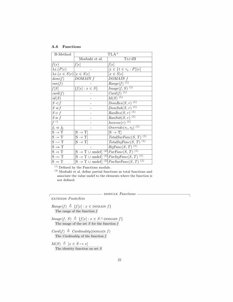
A.6 Functions

B-Method TLA+

Mosbahi et al. Tlc4B

f (e) f [e] f [e]λx .(P |e) - [x ∈ {t ∈ τx : P}|e]λx .(x ∈ S |e) [x ∈ S |e] [x ∈ S |e]dom(f ) DOMAIN f DOMAIN f

ran(f ) - Range(f ) (1)

f [S ] {f [x ] : x ∈ S} Image(f ,S ) (1)

card(f ) - Card(f ) (1)

id(S ) - Id(S ) (1)

S � f - DomRes(S , r) (1)

S �− f - DomSub(S , r) (1)

S � f - RanRes(S , r) (1)

S �− f - RanSub(S , r) (1)

f −1 - Inverse(r) (1)

f1 �− f2 - Override(r1, r2) (1)

S → T [S → T] [S → T]

S � T [S → T] TotalSurFunc(S ,T ) (1)

S � T [S → T] TotalInjFunc(S ,T ) (1)

S �� T - BijFunc(S ,T ) (1)

S 7→ T [S → T ∪ undef] (2) ParFunc(S ,T ) (1)

S 7� T [S → T ∪ undef] (2) ParInjFunc(S ,T ) (1)

S 7� T [S → T ∪ undef] (2) ParSurFunc(S ,T ) (1)

(1) Defined by the Functions module.(2) Mosbahi et al. define partial functions as total functions and

associate the value undef to the elements where the function isnot defined.

module Functionsextends FiniteSets

Range(f )∆= {f [x ] : x ∈ domain f }

The range of the function f

Image(f , S )∆= {f [x ] : x ∈ S ∩ domain f }

The image of the set S for the function f

Card(f )∆= Cardinality(domain f )

The Cardinality of the function f

Id(S )∆= [x ∈ S 7→ x ]

The identity function on set S

21

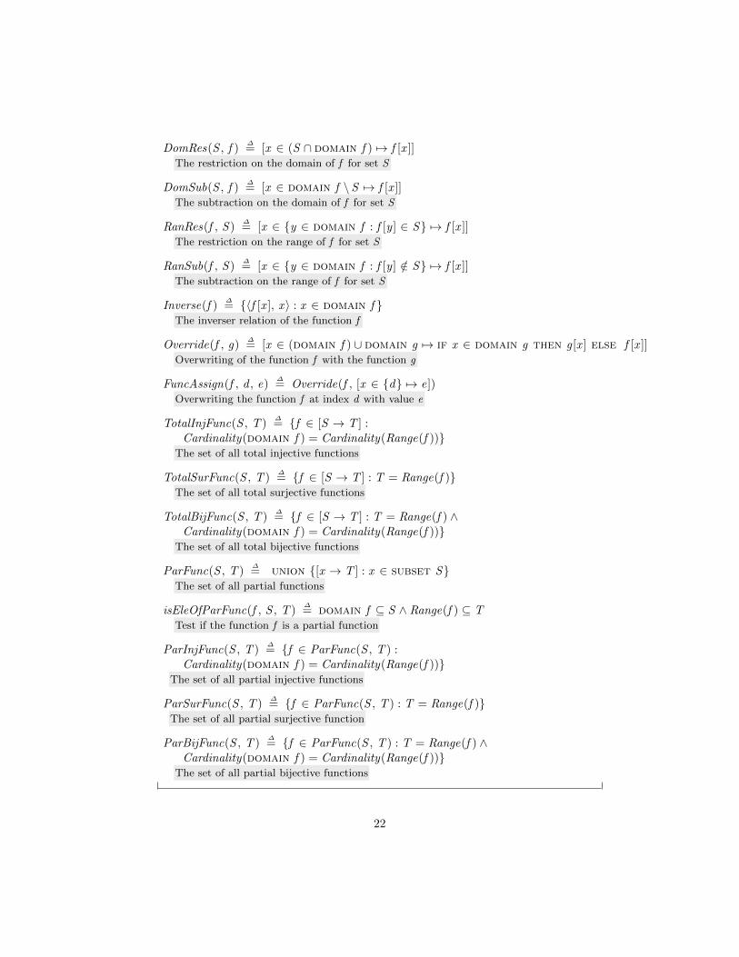
DomRes(S , f )∆= [x ∈ (S ∩ domain f ) 7→ f [x ]]

The restriction on the domain of f for set S

DomSub(S , f )∆= [x ∈ domain f \S 7→ f [x ]]

The subtraction on the domain of f for set S

RanRes(f , S )∆= [x ∈ {y ∈ domain f : f [y ] ∈ S} 7→ f [x ]]

The restriction on the range of f for set S

RanSub(f , S )∆= [x ∈ {y ∈ domain f : f [y ] /∈ S} 7→ f [x ]]

The subtraction on the range of f for set S

Inverse(f )∆= {〈f [x ], x 〉 : x ∈ domain f }

The inverser relation of the function f

Override(f , g)∆= [x ∈ (domain f ) ∪ domain g 7→ if x ∈ domain g then g [x ] else f [x ]]

Overwriting of the function f with the function g

FuncAssign(f , d , e)∆= Override(f , [x ∈ {d} 7→ e])

Overwriting the function f at index d with value e

TotalInjFunc(S , T )∆= {f ∈ [S → T ] :

Cardinality(domain f ) = Cardinality(Range(f ))}The set of all total injective functions

TotalSurFunc(S , T )∆= {f ∈ [S → T ] : T = Range(f )}

The set of all total surjective functions

TotalBijFunc(S , T )∆= {f ∈ [S → T ] : T = Range(f ) ∧

Cardinality(domain f ) = Cardinality(Range(f ))}The set of all total bijective functions

ParFunc(S , T )∆= union {[x → T ] : x ∈ subset S}

The set of all partial functions

isEleOfParFunc(f , S , T )∆= domain f ⊆ S ∧ Range(f ) ⊆ T

Test if the function f is a partial function

ParInjFunc(S , T )∆= {f ∈ ParFunc(S , T ) :

Cardinality(domain f ) = Cardinality(Range(f ))}The set of all partial injective functions

ParSurFunc(S , T )∆= {f ∈ ParFunc(S , T ) : T = Range(f )}

The set of all partial surjective function

ParBijFunc(S , T )∆= {f ∈ ParFunc(S , T ) : T = Range(f ) ∧

Cardinality(domain f ) = Cardinality(Range(f ))}The set of all partial bijective functions

22

A.7 Sequences

B-Method TLA+

Mosbahi et al. Tlc4B

[e1, e2, e3] - 〈e1, e2, e3〉[] - 〈〉seq(S ) - Seq(S ) (1)

seq1(S ) - Seq1(S ) (2)

iseq(S )-

ISeq(S ) (2)

ISeqEleOf (S ) (2)

iseq1(S )-

ISeq1(S ) (2)

ISeq1EleOf (S ) (2)

perm(S ) - Perm(S ) (2)

size(s) - Len(s) (1)

first(s) - Head(s) (1)

last(s) - Last(s) (2)

tail(s) - Tail(s) (1)

rev(s) - Reverse(s) (2)

st - s ◦ t (1)

e → s - Prepend(e, s) (2)

s ← e - Append(s, e) (1)

conc(s) - Conc(s) (2)

s ↑ n - TakeFirstElements(s,n) (2)

s ↓ n - DropFirstElements(s,n) (2)

(1) Defined by the Sequences standard module.(2) Defined by the SequencesExtended module.

module SequencesExtendedextends Naturals, FiniteSets, Sequences, TLC

local Range(f )∆= {f [x ] : x ∈ domain f }

Last(s)∆= s[Len(s)]

The last element of the sequence s

Front(s)∆= [i ∈ 1 . . (Len(s)− 1) 7→ s[i ]]

The sequence s without its last element.

Prepend(e, s)∆= [i ∈ 1 . . (Len(s) + 1) 7→ if i = 1 then e else s[i − 1]]

The Sequence obtained by inserting e at the front of sequence s

Reverse(s)∆= let l

∆= Len(s)

23

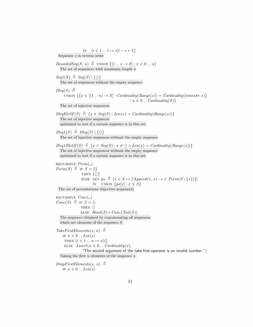
in [i ∈ 1 . . l 7→ s[l − i + 1]]Sequence s in reverse order

BoundedSeq(S , n)∆= union {[1 . . x → S ] : x ∈ 0 . . n}

The set of sequences with maximum length n

Seq1(S )∆= Seq(S ) \ {〈〉}

The set of sequences without the empty sequence

ISeq(S )∆=

union {{x ∈ [(1 . . n)→ S ] : Cardinality(Range(x )) = Cardinality(domain x )}: n ∈ 0 . . Cardinality(S )}

The set of injective sequences

ISeqEleOf (S )∆= {x ∈ Seq(S ) : Len(x ) = Cardinality(Range(x ))}

The set of injective sequences

optimized to test if a certain sequence is in this set.

ISeq1(S )∆= ISeq(S ) \ {〈〉}

The set of injective sequences without the empty sequence

ISeq1EleOf (S )∆= {x ∈ Seq(S ) : x 6= 〈〉 ∧ Len(x ) = Cardinality(Range(x ))}

The set of injective sequences without the empty sequence

optimized to test if a certain sequence is in this set.

recursive Perm( )Perm(S )

∆= if S = {}

then {〈〉}else let ps

∆= [x ∈ S 7→ {Append(s, x ) : s ∈ Perm(S \ {x})}]

in union {ps[x ] : x ∈ S}The set of permutations (bijective sequences)

recursive Conc( )Conc(S )

∆= if S = 〈〉

then 〈〉else Head(S ) ◦ Conc(Tail(S ))

The sequence obtained by concatenating all sequences

which are elements of the sequence S .

TakeFirstElements(s, n)∆=

if n ∈ 0 . . Len(s)then [i ∈ 1 . . n 7→ s[i ]]else Assert(n ∈ 0 . . Cardinality(s),

“The second argument of the take-first-operator is an invalid number.”)Taking the first n elements of the sequence s.

DropFirstElements(s, n)∆=

if n ∈ 0 . . Len(s)

24

then [i ∈ 1 . . (Len(s)− n) 7→ s[n + i ]]else Assert(n ∈ 0 . . Cardinality(s),

“The second argument of the drop-first-operator is an invalid number.”)Dropping the first n elements of the sequence s

A.8 Relations

B-Method TLA+

Mosbahi et al. Tlc4B

e 7→ f - 〈e, f 〉S ↔ T - Relations(S ,T ) (1)

dom(r) - RelDomain(r) (1)

ran(r) - RelRange(r) (1)

id(S ) - RelId(S ) (1)

S � r - RelDomRes(S , r) (1)

S �− r - RelDomSub(S , r) (1)

S � r - RelRanRes(S , r) (1)

S �− r - RelRanSub(S , r) (1)

r−1 - RelInverse(r) (1)

r [S ] - RelImage(r ,S ) (1)

r1 �− r2 - RelOverride(r1, r2) (1)

r1 ⊗ r2 - RelDirectProduct(r1, r2) (1)

r1; r2 - RelComposition(r1, r2) (1)

r1 ‖ r2 - RelParallelProd(r1, r2) (1)

prj1(S ,T ) - RelPrj1(S ,T ) (1)

prj2(S ,T ) - RelPrj2(S ,T ) (1)

r+ - RelClosure1(r) (1)

r∗ - RelClosure(r) (1)

rn - RelIterate(r ,n) (1)

fnc(r) - RelFnc(r) (1)

rel(r) - RelRel(r) (1)

(1) Defined by the Relations module.

module Relationsextends FiniteSets, Naturals, Sequences, TLC

Relations(S , T )∆= subset (S × T )

The set of all relations

RelDomain(R)∆= {x [1] : x ∈ R}

The domain of the relation R

25

RelRange(R)∆= {x [2] : x ∈ R}

The range of the relation R

RelId(S )∆= {〈x , x 〉 : x ∈ S}

The identity relation of set S

RelDomRes(S , R)∆= {x ∈ R : x [1] ∈ S}

The restriction on the domain of R for set S

RelDomSub(S , R)∆= {x ∈ R : x [1] /∈ S}

The subtraction on the domain of R for set S

RelRanRes(R, S )∆= {x ∈ R : x [2] ∈ S}

The restriction on the range of R for set S

RelRanSub(R, S )∆= {x ∈ R : x [2] /∈ S}

The subtraction on the range of R for set S

RelInverse(R)∆= {〈x [2], x [1]〉 : x ∈ R}

The reverse relation of R

RelImage(R, S )∆= {y [2] : y ∈ {x ∈ R : x [1] ∈ S}}

The image of R for set S

RelOverride(R1, R2)∆= {x ∈ R1 : x [1] /∈ RelDomain(R2)} ∪ R2

Overwriting relation R1 with R2

RelComposition(R1, R2)∆= {〈u[1][1], u[2][2]〉 : u ∈

{x ∈ RelRanRes(R1, RelDomain(R2))× RelDomRes(RelRange(R1), R2) :x [1][2] = x [2][1]}}

The relational composition of R1 and R2

RelDirectProduct(R1, R2)∆= {〈x , u〉 ∈ RelDomain(R1)× (RelRange(R1)× RelRange(R2)) :

∧ 〈x , u[1]〉 ∈ R1∧ 〈x , u[2]〉 ∈ R2}

The direct product of relation R1 and R2

RelParallelProduct(R1, R2)∆= {〈a, b〉 ∈ (RelDomain(R1)× RelDomain(R2))

× (RelRange(R1)× RelRange(R2)): 〈a[1], b[1]〉 ∈ R1 ∧ 〈a[2], b[2]〉 ∈ R2}

The parallel product of R1 and R2

RelPrj 1(S , T )∆= {〈〈a, b〉, a〉 : a ∈ S , b ∈ T}

The first projection relation

RelPrj 2(S , T )∆= {〈〈a, b〉, b〉 : a ∈ S , b ∈ T}

The second projection relation

recursive RelIterate( , )

26

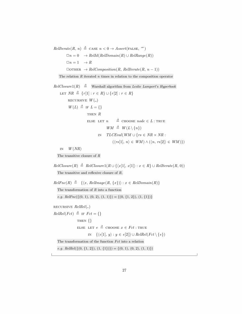
RelIterate(R, n)∆= case n < 0→ Assert(false, “”)

2n = 0 → RelId(RelDomain(R) ∪ RelRange(R))

2n = 1 → R

2other → RelComposition(R, RelIterate(R, n − 1))

The relation R iterated n times in relation to the composition operator

RelClosure1(R)∆= Warshall algorithm from Leslie Lamport ’s Hyperbook

let NR∆= {r [1] : r ∈ R} ∪ {r [2] : r ∈ R}

recursive W ( )

W (L)∆= if L = {}

then R

else let n∆= choose node ∈ L : true

WM∆= W (L \ {n})

in TLCEval(WM ∪ {rs ∈ NR ×NR :

(〈rs[1], n〉 ∈ WM ) ∧ (〈n, rs[2]〉 ∈ WM )})

in W (NR)

The transitive closure of R

RelClosure(R)∆= RelClosure1(R ∪ {〈x [1], x [1]〉 : x ∈ R} ∪ RelIterate(R, 0))

The transitive and reflexive closure of R.

RelFnc(R)∆= {〈x , RelImage(R, {x})〉 : x ∈ RelDomain(R)}

The transformation of R into a function

e.g . RelFnc({(0, 1), (0, 2), (1, 1)}) = {(0, {1, 2}), (1, {1})}

recursive RelRel( )

RelRel(Fct)∆= if Fct = {}

then {}

else let e∆= choose x ∈ Fct : true

in {〈e[1], y〉 : y ∈ e[2]} ∪ RelRel(Fct \ {e})

The transformation of the function Fct into a relation

e.g . RelRel({(0, {1, 2}), (1, {1})}) = {(0, 1), (0, 2), (1, 1)})

27

A.9 Functions as Relations

B-Method TLA+

Mosbahi et al. Tlc4B

f (e) - RelCall(f , e) (1)

λx .(P |e) - {〈x , e〉 : x ∈ {t ∈ τx : P}λx .(x ∈ S |e) - {〈x , e〉 : x ∈ S}S → T

-RelTotalFunc(S ,T ) (1)

RelTotalFuncEleOf (S ,T ) (1)

S � T-

RelTotalSurFunc(S ,T ) (1)

RelTotalSurFuncEleOf (S ,T ) (1)

S � T-

RelTotalInjFunc(S ,T ) (1)

RelTotalInjFuncEleOf (S ,T ) (1)

S �� T-

RelTotalBijFunc(S ,T ) (1)

RelTotalBijFuncEleOf (S ,T ) (1)

S 7→ T-

RelParFunc(S ,T ) (1)

RelParFuncEleOf (S ,T ) (1)

S 7� T-

RelParInjFunc(S ,T ) (1)

RelParInjFuncEleOf (S ,T ) (1)

S 7� T-

RelParSurFunc(S ,T ) (1)

RelParSurFuncEleOf (S ,T ) (1)

S 7� T-

RelParBijFunc(S ,T ) (1)

RelParBijFuncEleOf (S ,T ) (1)

(1) Defined by the FunctionsAsRelations module.

module FunctionsAsRelationsextends FiniteSets, Functions, TLC , Sequences

local RelDom(f )∆= {x [1] : x ∈ f } The domain of the function

local RelRan(f )∆= {x [2] : x ∈ f } The range of the function

local MakeRel(f )∆= {〈x , f [x ]〉 : x ∈ domain f }

Converting a TLA+ function to a set of pairs

local Rel(S , T )∆= subset (S × T ) The set of relations

local IsFunc(f )∆= Cardinality(RelDom(f )) = Cardinality(f )

Testing if f is a function

local IsTotal(f , dom)∆= RelDom(f ) = dom

Testing if f is a total function

local IsInj (f )∆= Cardinality(RelRan(f )) = Cardinality(f )

Testing if f is a injective function

local IsSurj (f , ran)∆= RelRan(f ) = ran

Testing if f is a surjective function

RelCall(f , x )∆= if Cardinality(f ) = Cardinality(RelDom(f )) ∧ x ∈ RelDom(f )

28

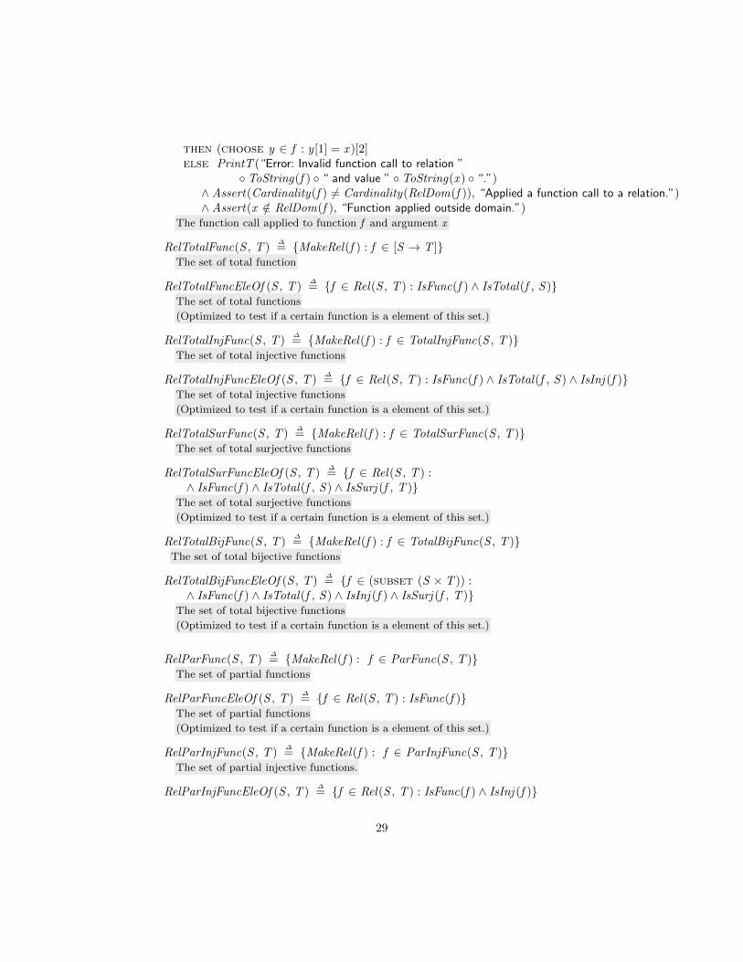
then (choose y ∈ f : y [1] = x )[2]else PrintT (“Error: Invalid function call to relation ”

◦ ToString(f ) ◦ “ and value ” ◦ ToString(x ) ◦ “.”)∧Assert(Cardinality(f ) 6= Cardinality(RelDom(f )), “Applied a function call to a relation.”)∧Assert(x /∈ RelDom(f ), “Function applied outside domain.”)

The function call applied to function f and argument x

RelTotalFunc(S , T )∆= {MakeRel(f ) : f ∈ [S → T ]}

The set of total function

RelTotalFuncEleOf (S , T )∆= {f ∈ Rel(S , T ) : IsFunc(f ) ∧ IsTotal(f , S )}

The set of total functions

(Optimized to test if a certain function is a element of this set.)

RelTotalInjFunc(S , T )∆= {MakeRel(f ) : f ∈ TotalInjFunc(S , T )}

The set of total injective functions

RelTotalInjFuncEleOf (S , T )∆= {f ∈ Rel(S , T ) : IsFunc(f ) ∧ IsTotal(f , S ) ∧ IsInj (f )}

The set of total injective functions

(Optimized to test if a certain function is a element of this set.)

RelTotalSurFunc(S , T )∆= {MakeRel(f ) : f ∈ TotalSurFunc(S , T )}

The set of total surjective functions

RelTotalSurFuncEleOf (S , T )∆= {f ∈ Rel(S , T ) :

∧ IsFunc(f ) ∧ IsTotal(f , S ) ∧ IsSurj (f , T )}The set of total surjective functions

(Optimized to test if a certain function is a element of this set.)

RelTotalBijFunc(S , T )∆= {MakeRel(f ) : f ∈ TotalBijFunc(S , T )}

The set of total bijective functions

RelTotalBijFuncEleOf (S , T )∆= {f ∈ (subset (S × T )) :

∧ IsFunc(f ) ∧ IsTotal(f , S ) ∧ IsInj (f ) ∧ IsSurj (f , T )}The set of total bijective functions

(Optimized to test if a certain function is a element of this set.)

RelParFunc(S , T )∆= {MakeRel(f ) : f ∈ ParFunc(S , T )}

The set of partial functions

RelParFuncEleOf (S , T )∆= {f ∈ Rel(S , T ) : IsFunc(f )}

The set of partial functions

(Optimized to test if a certain function is a element of this set.)

RelParInjFunc(S , T )∆= {MakeRel(f ) : f ∈ ParInjFunc(S , T )}

The set of partial injective functions.

RelParInjFuncEleOf (S , T )∆= {f ∈ Rel(S , T ) : IsFunc(f ) ∧ IsInj (f )}

29

The set of partial injective functions

(Optimized to test if a certain function is a element of this set.)

RelParSurFunc(S , T )∆= {MakeRel(f ) : f ∈ ParSurFunc(S , T )}

The set of partial surjective functions

RelParSurFuncEleOf (S , T )∆= {f ∈ Rel(S , T ) : IsFunc(f ) ∧ IsSurj (f , T )}

The set of partial surjective functions.

(Optimized to test if a certain function is a element of this set.)

RelParBijFunc(S , T )∆= {MakeRel(f ) : f ∈ ParBijFunc(S , T )}

The set of partial bijective functions

RelParBijFuncEleOf (S , T )∆= {f ∈ Rel(S , T ) : IsFunc(f ) ∧ IsSurj (f , T ) ∧ IsInj (f )}

The set of partial bijective functions

(Optimized to test if a certain function is a element of this set.)

30

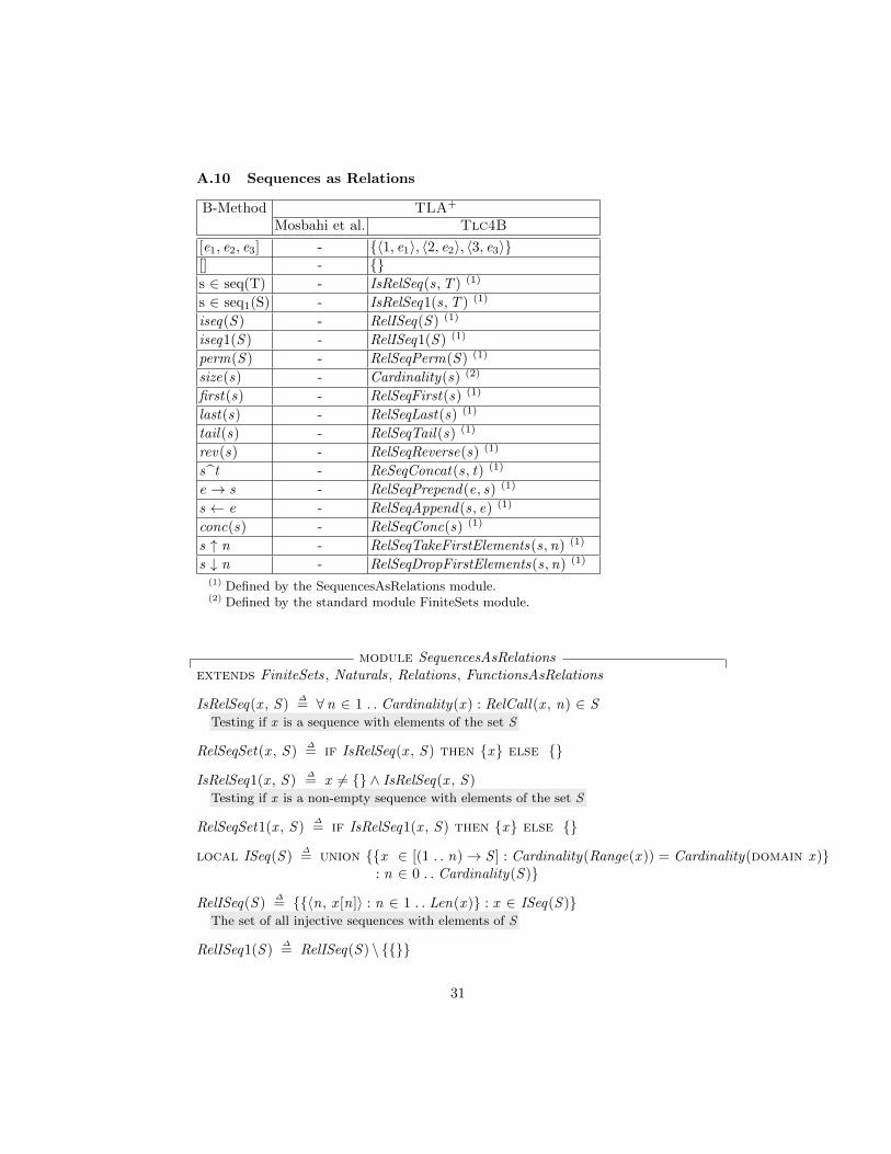
A.10 Sequences as Relations

B-Method TLA+

Mosbahi et al. Tlc4B

[e1, e2, e3] - {〈1, e1〉, 〈2, e2〉, 〈3, e3〉}[] - {}s ∈ seq(T) - IsRelSeq(s,T ) (1)

s ∈ seq1(S) - IsRelSeq1(s,T ) (1)

iseq(S ) - RelISeq(S ) (1)

iseq1(S ) - RelISeq1(S ) (1)

perm(S ) - RelSeqPerm(S ) (1)

size(s) - Cardinality(s) (2)

first(s) - RelSeqFirst(s) (1)

last(s) - RelSeqLast(s) (1)

tail(s) - RelSeqTail(s) (1)

rev(s) - RelSeqReverse(s) (1)

st - ReSeqConcat(s, t) (1)

e → s - RelSeqPrepend(e, s) (1)

s ← e - RelSeqAppend(s, e) (1)

conc(s) - RelSeqConc(s) (1)

s ↑ n - RelSeqTakeFirstElements(s,n) (1)

s ↓ n - RelSeqDropFirstElements(s,n) (1)

(1) Defined by the SequencesAsRelations module.(2) Defined by the standard module FiniteSets module.

module SequencesAsRelationsextends FiniteSets, Naturals, Relations, FunctionsAsRelations

IsRelSeq(x , S )∆= ∀n ∈ 1 . . Cardinality(x ) : RelCall(x , n) ∈ S

Testing if x is a sequence with elements of the set S

RelSeqSet(x , S )∆= if IsRelSeq(x , S ) then {x} else {}

IsRelSeq1(x , S )∆= x 6= {} ∧ IsRelSeq(x , S )

Testing if x is a non-empty sequence with elements of the set S

RelSeqSet1(x , S )∆= if IsRelSeq1(x , S ) then {x} else {}

local ISeq(S )∆= union {{x ∈ [(1 . . n)→ S ] : Cardinality(Range(x )) = Cardinality(domain x )}

: n ∈ 0 . . Cardinality(S )}

RelISeq(S )∆= {{〈n, x [n]〉 : n ∈ 1 . . Len(x )} : x ∈ ISeq(S )}

The set of all injective sequences with elements of S

RelISeq1(S )∆= RelISeq(S ) \ {{}}

31

The set of all non-empty injective sequences with elements of S

local SeqTest(s)∆= RelDomain(s) = 1 . . Cardinality(s)

Testing if s is a sequence

RelSeqFirst(s)∆= if SeqTest(s)

then RelCall(s, 1)else Assert(false, “Error: The argument of the first-operator should be a sequence.”)

The head of the sequence

RelSeqLast(s)∆= if SeqTest(s)

then RelCall(s, Cardinality(s))else Assert(false, “Error: The argument of the last-operator should be a sequence.”)

The last element of the sequence

RelSeqSize(s)∆= if SeqTest(s)

then Cardinality(s)else Assert(false, “Error: The argument of the size-operator should be a sequence.”)

The size of the sequence s

RelSeqTail(s)∆= if SeqTest(s)

then {〈x [1]− 1, x [2]〉 : x ∈ {x ∈ s : x [1] 6= 1}}else Assert(false, “Error: The argument of the tail-operator should be a sequence.”)

The tail of the sequence s

RelSeqConcat(s1, s2)∆= if SeqTest(s1) ∧ SeqTest(s2)

then s1 ∪ {〈x [1] + Cardinality(s1), x [2]〉 : x ∈ s2}else Assert(false, “Error: The arguments of the concatenation-operator should be sequences.”)

The concatenation of sequence s1 and sequence s2

RelSeqPrepand(e, s)∆= if SeqTest(s)

then {〈1, e〉} ∪ {〈x [1] + 1, x [2]〉 : x ∈ s}else Assert(false, “Error: The second argument of the prepend-operator should be a sequence.”)

The sequence obtained by inserting e at the front of sequence s.

RelSeqAppend(s, e)∆= if SeqTest(s)

then s ∪ {〈Cardinality(s) + 1, e〉}else Assert(false, “Error: The first argument of the append-operator should be a sequence.”)

The sequence obtained by appending e to the end of sequence s.

RelSeqReverse(s)∆= if SeqTest(s)

then {〈Cardinality(s)− x [1] + 1, x [2]〉 : x ∈ s}else Assert(false, “Error: The argument of the reverse-operator should be a sequence.”)

The sequence obtained by reversing the order of the elements.

RelSeqFront(s)∆= if SeqTest(s)

then {x ∈ s : x [1] 6= Cardinality(s)}else Assert(false, “Error: The argument of the front-operator should be a sequence.”)

32

The front of the sequence s (all but last element)

recursive RelSeqPerm( )

RelSeqPerm(S )∆= if S = {}

then {{}}else let ps

∆= [x ∈ S 7→ {RelSeqAppend(s, x ) : s ∈ RelSeqPerm(S \ {x})}]

in union {ps[x ] : x ∈ S}The set of bijective sequences (permutations)

e.g . {〈1, 2, 3〉, 〈2, 1, 3〉, 〈2, 3, 1〉, 〈3, 1, 2〉, 〈3, 2, 1〉} for S = {1, 2, 3}

recursive RelSeqConc( )

RelSeqConc(S )∆=

if S = {}then {}else RelSeqConcat(RelSeqFirst(S ), RelSeqConc(RelSeqTail(S )))

The sequence obtained by concatenating all sequences

which are elements of the sequence S .

RelSeqTakeFirstElements(s, n)∆=

if SeqTest(s) ∧ n ∈ 0 . . Cardinality(s)

then {x ∈ s : x [1] ≤ n}else ∧Assert(n ∈ 0 . . Cardinality(s),

“The second argument of the take-first-operator is an invalid number.”)

∧Assert(false, “Error: The first argument of the take-first-operator should be a sequence.”)

The first n elements of s as a sequence

RelSeqDropFirstElements(s, n)∆=

if SeqTest(s) ∧ n ∈ 0 . . Cardinality(s)

then {〈x [1]− n, x [2]〉 : x ∈ {x ∈ s : x [1] > n}}else ∧Assert(n ∈ 0 . . Cardinality(s),

“The second argument of the drop-first-operator is an invalid number.”)

∧Assert(false, “Error: The first argument of the drop-first-operator should be a sequence.”)

The last n elements of s as a sequence

A.11 Strings

B-Method TLA+

Mosbahi et al. Tlc4B

“abc” - “abc”STRING - STRING

33

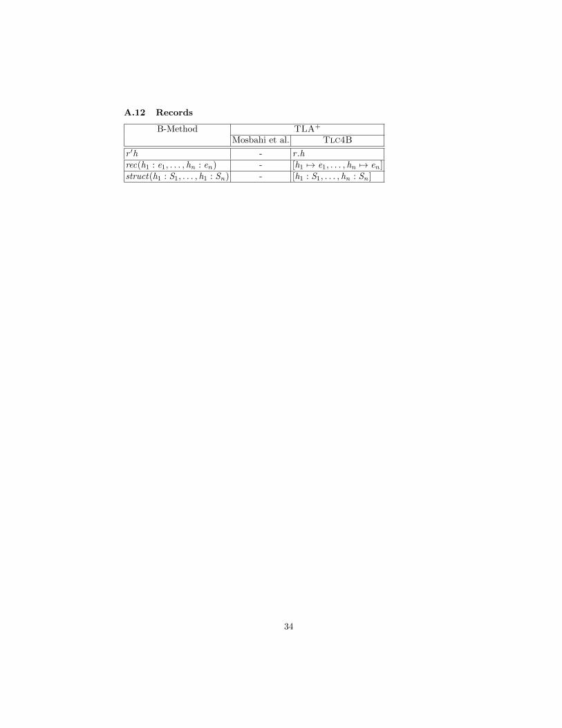
A.12 Records

B-Method TLA+

Mosbahi et al. Tlc4B

r ′h - r .hrec(h1 : e1, . . . , hn : en) - [h1 7→ e1, . . . , hn 7→ en ]struct(h1 : S1, . . . , h1 : Sn) - [h1 : S1, . . . , hn : Sn ]

34

References

1. J.-R. Abrial. The B-Book. Cambridge University Press, 1996.2. K. Chaudhuri, D. Doligez, L. Lamport, and S. Merz. The TLA+ proof system: Build-

ing a heterogeneous verification platform. In A. Cavalcanti, D. Deharbe, M.-C. Gaudel,and J. Woodcock, editors, Proceedings ICTAC 2010, LNCS 6255, page 44, 2010.

3. ClearSy. B language reference manual. http://www.tools.clearsy.com/resources/Manrefb_en.pdf. Accessed: 2013-11-10.

4. E. Gafni and L. Lamport. Disk paxos. Distributed Computing, 16(1):1–20, 2003.5. D. Hansen and M. Leuschel. Translating TLA+ to B for validation with ProB. In

Proceedings iFM’2012, LNCS 7321, pages 24–38. Springer, 2012.6. D. Hansen and M. Leuschel. Translating B to TLA+ for validation with TLC: There

and back again. http://www.stups.uni-duesseldorf.de/w/Special:Publication/

HansenLeuschel_TLC4B_techreport, 2013.

7. L. Lamport. The TLA+ hyperbook. http://research.microsoft.com/en-us/um/

people/lamport/tla/hyperbook.html. Accessed: 2013-10-30.8. L. Lamport. Specifying Systems, The TLA+ Language and Tools for Hardware and

Software Engineers. Addison-Wesley, 2002.9. M. Leuschel and M. Butler. ProB: A model checker for B. In K. Araki, S. Gnesi,

and D. Mandrioli, editors, FME 2003: Formal Methods, LNCS 2805, pages 855–874.Springer-Verlag, 2003.

10. M. Leuschel and M. J. Butler. ProB: an automated analysis toolset for the B method.STTT, 10(2):185–203, 2008.

11. O. Mosbahi, L. Jemni, and J. Jaray. A formal approach for the development ofautomated systems. In J. Filipe, B. Shishkov, and M. Helfert, editors, ICSOFT (SE),pages 304–310. INSTICC Press, 2007.

12. M. Reynolds. Changing nothing is sometimes doing something. Technical ReportTR-98-02, Department of Computer Science, King’s College London, February 1998.

13. Y. Yu, P. Manolios, and L. Lamport. Model checking TLA+ specifications. In L. Pierreand T. Kropf, editors, Proceedings CHARME’99, LNCS 1703, pages 54–66. Springer-Verlag, 1999.

35