Transient thermal conduction with variable conductivity ...€¦ · A numerical solution of the...

Applied Mathematics and Computation xxx (2015) xxx–xxx

Contents lists available at ScienceDirect

Applied Mathematics and Computation

journal homepage: www.elsevier .com/ locate/amc

Transient thermal conduction with variable conductivity usingthe Meshless Local Petrov–Galerkin method

http://dx.doi.org/10.1016/j.amc.2015.02.0840096-3003/� 2015 Elsevier Inc. All rights reserved.

⇑ Corresponding author at: Institute of Chemical Engineering Sciences (ICEHT), Foundation for Research and Technology, Hellas (FORTH), GPatras, Greece.

E-mail address: [email protected] (E.D. Skouras).

Please cite this article in press as: N.P. Karagiannakis et al., Transient thermal conduction with variable conductivity using the MLocal Petrov–Galerkin method, Appl. Math. Comput. (2015), http://dx.doi.org/10.1016/j.amc.2015.02.084

N.P. Karagiannakis a, G.C. Bourantas b,c, A.N. Kalarakis b, E.D. Skouras b,a,⇑, V.N. Burganos a

a Institute of Chemical Engineering Sciences (ICEHT), Foundation for Research and Technology, Hellas (FORTH), GR-26504 Patras, Greeceb TEI of Western Greece, Department of Mechanical Engineering, M. Alexandrou 1, Patras, Greecec Faculty of Science, Technology and Communication, University of Luxembourg, Luxembourg

a r t i c l e i n f o a b s t r a c t

Keywords:Meshless Petrov–GalerkinMoving Least SquaresHeat conductionSpatiotemporally varying conductivity

A numerical solution of the transient heat conduction problem with spatiotemporally vari-able conductivity in 2D space is obtained using the Meshless Local Petrov–Galerkin (MLPG)method. The approximation of the field variables is performed using Moving Least Squares(MLS) interpolation. The accuracy and the efficiency of the MLPG schemes are investigatedthrough variation of (i) the domain resolution, (ii) the order of the basis functions, (iii) theshape of the integration site around each node, (iv) the conductivity range, and (v) thevolumetric heat capacity range. Steady-state boundary conditions of the essential typeare assumed. The results are compared with those calculated by a typical Finite Elementmethod. Specific rectangular-type integration sites are introduced during both steady-stateand transient MLPG integration, in order to provide complete surface coverage of thedomain without overlapping, and the accuracy of the method is demonstrated in all casesstudied. Computational efficiency is also investigated with this MLPG method and found tobe slower than FE methods during construction stage, but it clearly surpasses that of FEMapproaches during the solution stage on a wide parameter range.

� 2015 Elsevier Inc. All rights reserved.

1. Introduction

The subject of heat transfer is of fundamental importance in numerous areas of engineering science involving energytransport in processes driven by temperature differences [1,2]. Transient heat transfer studies provide vital cost-effectiveand efficient solutions for many modern critical applications, as in modeling of heat transport within biological tissues,which is of direct interest to various therapeutic applications [2]. Variable conductivity can be observed in medicinal appli-cations such as laser ablation of tumors and biological tissues, as well as industrial applications with liquid metals [3],stretching sheets [4], and crystallinity effects on amorphous polymers [5].

The Finite Element method using the Galerkin description has found extensive engineering acceptance as well as vastcommercialization, due to its origins in generalized variational principles and its convenience. Compared with its suitabilityand flexibility in broad use, the Finite Element method has been long criticized for inherent problems such as complex mesh-ing and remeshing problems, connectivity issues, and poor derivatives. Such conventional CFD numerical techniquesordinarily utilized in heat transfer studies still have these inherent deficiencies that lower their effectiveness and reduce

R-26504

eshless

http://dx.doi.org/10.1016/j.amc.2015.02.084

mailto:[email protected]


http://www.sciencedirect.com/science/journal/00963003

http://www.elsevier.com/locate/amc


2 N.P. Karagiannakis et al. / Applied Mathematics and Computation xxx (2015) xxx–xxx

their applicability to practical applications, particularly those involving complex transient problems. The main source of defi-ciency is related to the requirement of a well-organized and connected mesh in the problem domain and the boundaries. Themesh creation can be highly difficult, usually requiring time-consuming user involvement. Domain mesh generation can beavoided with the application of Boundary Element Methods (BEM), another class of methods broadly applied in heat transferengineering. However, BEM is usually constrained to cases where the infinite space fundamental solution for the differentialoperator is available, and the evaluation of the unknown field variable and/or its gradients at any single point within thedomain of the problem involves tedious calculations of integrals over the global boundaries. Both FEM and BEM unavoidablyhave to handle the nonlinear terms during the solution of nonlinear cases.

A more attractive alternative for such tasks is a meshless discretization approach using finite point approximations,which are gradually becoming well-established in recent years. Several meshless methods have been reported thus far, suchas the Diffuse Element Method (DEM) [6], the Element Free Galerkin (EFG) method [7–9], and the Reproducing KernelParticle (RKP) method [10]. Meshless methods have undergone extensive development recently, largely due to their inherentpotential of handling engineering problems with complex and irregular geometries more efficiently than standard com-putational techniques [11]. Meshless numerical techniques rely on local type interpolation on either regularly or irregularlydistributed spatial points, usually called nodes. Their main advantage over traditional mesh-based numerical methods is thefact that usually there is no need for a mesh and for definition of the connectivity between adjacent elements. In this way,the effort devoted to mesh generation is reduced considerably, since PDE linearization and interpolation is performed interms of the nodal points distributed on the problem domain. However, most of these methods still need ‘‘shadow’’ elementsto integrate over the entire domain of the problem for integral properties, such as energy or fluxes, and so far, have beenapplied mainly to solve linear problems.

Linear heat transfer problems have been addressed with meshless methods in a number of heat conduction studies. Thetransient heat conduction behavior of functionally graded anisotropic materials with continuously variable material proper-ties have been investigated with the application of meshless local boundary integral equations with Moving Least-Squaresapproximations using Laplace transformation for the time integration of 2D problems [12,13], whereas anisotropic linearly-graded transient three-dimensional problems, either axisymmetric [14], or fully 3D [15], have been efficiently tackled in asimilar fashion using Meshless Local Petrov–Galerkin methods.

This truly meshless formulation based on the recently developed [16] local symmetric weak form with the Local Petrov–Galerkin approach is proposed here to solve transient non-linear heat conduction problems. The essential boundary condi-tions in the present formulation were imposed by 1st order MLS description. This method does not need elements or meshes,either for interpolation purposes, or for integration purposes. All integrals are carried out only on circles (in 2-D, or spheres in3-D) centered at each point in question, or in rectangles (in 2-D, or orthorhombic parallelepipeds in 3-D). The presentmethod is also more flexible and easier in dealing with nonlinear problems than the conventional FEM, EFG and BEM.

In the present work, 2-D thermal conduction problems with spatiotemporally variable conductivity are solved (Fig. 1(a)),although the methodology can be straightforwardly extended to 3-D applications. The Meshless Local Petrov–Galerkin(MLPG) method is used to discretize the problems using Moving Least-Squares (MLS) approximations. The effect of severalkey parameters on the accuracy and efficiency of the numerical solutions is examined, such as (i) the domain resolution (100px, 200 px, or refinement), (ii) the order of the basis function used (1st or 2nd), (iii) the shape of the integration site around

(a) (b)Fig. 1. (a) Rectangular MLPG integration scheme with the Gauss points of integration around characteristic nodes. (b) Refinement in MLPG scheme. Bluepoints: basic nodes (at 100 px) with rectangular integration applied; green points: ‘‘bulky’’ refined nodes (at 200 px) near conductivity interfaces withrectangular integration applied; red points: locally refined nodes (at 200 px) at bulky refinement edges with circular integration applied; stars: limits(Gauss points) of the integration around respective nodes. (For interpretation of the references to color in this figure legend, the reader is referred to the webversion of this article.)

Please cite this article in press as: N.P. Karagiannakis et al., Transient thermal conduction with variable conductivity using the MeshlessLocal Petrov–Galerkin method, Appl. Math. Comput. (2015), http://dx.doi.org/10.1016/j.amc.2015.02.084


N.P. Karagiannakis et al. / Applied Mathematics and Computation xxx (2015) xxx–xxx 3

each node used (circular or rectangular), and (iv) the conductivity and (v) the volumetric heat capacity ranges of the media.The collocation-based meshfree approach does not require any grid mesh, except for a set of distributed nodes in the spatialdomain [17,18]. Thus, when it comes to complex geometries, this method may have advantages over the conventional FDMand FEM ones, or even more sophisticated methods such as the Lattice-Boltzmann method [18]. The results obtained hereinare compared with those of ordinary FEM solutions applied to the same physical problem [19–21].

2. Methods

A truly meshless method, based on the MLPG approach and the Moving Least Squares approximation is presented herein,for solving transient heat convection problems with increased accuracy. The present method makes no use of a ‘‘finite ele-ment mesh’’, either for purposes of interpolation of the solution variables, or for integration during calculation of energy orfluxes. All integrals can be easily evaluated over regularly shaped domains (in general, spheres in three-dimensional prob-lems) and their boundaries. No post-smoothing technique is required for computing the derivatives of the unknown variable,since the original solution, using the Moving Least Squares approximation, is already sufficiently smooth. Several numericalexamples are presented in the paper. In essence, the present meshless method based on the MLPG is found to be a simple,efficient, and attractive method with a great potential in engineering applications.

The solution approximation, Th(x), is described following the Moving Least Squares technique [20,22], as the product of avector of polynomial base, p(x), and a vector of coefficients, a(x).

PleaseLocal

ThðxÞ ¼ pTðxÞaðxÞ ð1Þ

where pðxÞ;aðxÞ 2 Rq, and q is the number of monomials in the polynomial bases (here, 3 or 6). The local characteristics of theMLS approximation can be considered as a generalization of the traditional least-squares approximation, where the coeffi-cients a are independent of the local position, x.

Eq. (1) is referred to as the global least-squares approximation, however, a unique local approximation associated witheach point in the domain can also be described. In order to determine the form of a(x), a weighted discrete error norm isconstructed and minimized.

JðxÞ ¼Xn

I¼1

wIðxÞXm

j¼1

pTj ðxIÞaðxÞ � TI

" #2

; ð2Þ

wI(x) denotes the weight function, wI(x) � wI(x � xI), associated with node I, while the quantity in brackets is the differencebetween the local approximation at node I and the field data at node I, TI, and n is the number of nodes in the support of wI(x).Minimization of Eq. (2) with respect to a(x) determines the latter and results in the following linear system

AðxÞaðxÞ ¼ BðxÞTs: ð3Þ

Ts is a vector containing the nodal data, and A;B 2 Rm�n are matrix functions of wI(x) and p(xI). Substitution of the solution ofEq. (3) into the global approximation, Eq. (1), completes the least-squares approximation. Derivatives of the shape function,

/ðxÞ ¼ pTðxÞA�1ðxÞBðxÞ, can be calculated with the product rule.The weighted integral of the transient heat conduction equation at the domain Xx around point x is given as
Z
Xx

~q~cp@~T@~t� ~r � ð~k ~r~TÞ

" #wdXx ¼ 0; ð4Þ

with weight function w = 1 where x e Xx, and 0 elsewhere. Tildes in notation imply dimensional quantities. The 2nd term(conduction) of Eq. (4) can be integrated by parts and the Gauss theorem can be used to obtain the following weak symmet-ric formulation:
Z
Xx

~r � ð~k ~r~TÞwdXx ¼Z@Xx

~k ~r~T n̂wdð@XxÞ �Z

Xx

~k ~r~T ~rwdXx; ð5Þ

where @Xx is the boundary of the domain Xx. With the given weight function the last term in Eq. (5) is inherently zero. Timederivatives (1st term of Eq. (4)) can be written in a Crank–Nicholson scheme, however these integrals cannot be downsizedusing the Gauss theorem. The robustness of the method is increased significantly when the resulting non-linear terms aredescribed in a semi-explicit formulation (at time step m) of the following type:

~TðmÞ ~r~TðmÞ ¼ ~TðmÞ ~r~Tðm�1Þ þ ~Tðm�1Þ ~r~TðmÞ � ~Tðm�1Þ ~r~T ðm�1Þ: ð6Þ

The conductivity, ~k, which is assumed dependent on temperature (first-order dependence in this work, however straight-forwardly applicable to more complex descriptions), and the volumetric heat capacity, ~q~cp, are defined as:

~k ¼~k1 þ ~b1

~T; x 2 X1

~k2 þ ~b2~T; x 2 X2

( ); ð7Þ

cite this article in press as: N.P. Karagiannakis et al., Transient thermal conduction with variable conductivity using the MeshlessPetrov–Galerkin method, Appl. Math. Comput. (2015), http://dx.doi.org/10.1016/j.amc.2015.02.084



PleaseLocal

~q~cp ¼~q1~cp1; x 2 X1

~q2~cp2; x 2 X2

� �: ð8Þ

Reduced quantities are determined based on the domain geometry and the boundary conditions,

x ¼~x~L; y ¼

~y~L; T ¼

~T � ~T2

~T1 � ~T2

; ð9Þ

and on the physical values of medium 1, as well:

t ¼~t~k1

~q1~c1~L2; ð10Þ

k ¼~k~k1

¼1þ b1T; x 2 X1

kr þ b2T; x 2 X2

� �; ð11Þ

qcp ¼~q~cp

~q1~cp1¼

1; x 2 X1

qcp;r; x 2 X2

� �: ð12Þ

Dimensionless characteristic constants of the process are defined as:

kr ¼~k2

~k1

; b1 ¼~b1

~k1

; b2 ¼~b2

~k1

; br ¼b2

b1; qcp;r ¼

q2cp2

q1cp1; ar ¼

kr

qcp;r: ð13Þ

kr is the ratio of the temperature-independent parts of the conductivity descriptions, while br is the ratio of the temperature-dependent respective parts. X1 and X2 are the domains of medium 1 (exterior) and 2 (interior) of the enclosure. If U is thestep function defined at the domain of the interior medium (unit there, zero elsewhere), the reduced coefficients can belinearized as:

k ¼ ðkr � 1ÞUþ 1þ b1½~T2 þ ð~T1 � ~T2ÞT�ðbr � 1ÞUþ b1½~T2 þ ð~T1 � ~T2ÞT�; ð14Þ

qcp ¼ ðqcp;r � 1ÞUþ 1: ð15Þ

The iterative form of Eq. (5) can now be written as follows.

ðqcp;r � 1ÞZ

Xx

UTðmÞ � Tðm�1Þ

DtdXx þ

ZXx

TðmÞ � Tðm�1Þ

DtdXx � ½kr � 1þ b1

~T2ðbr � 1Þ�Z@Xx

UrTðmÞn̂ dð@XxÞ

� ð1þ b1~T2ÞZ@Xx

rTðmÞn̂ dð@XxÞ � b1ð~T1 � ~T2Þðbr � 1ÞZ@Xx

U T ðmÞrTðmÞn̂ dð@XxÞ � b1ð~T1 � ~T2ÞZ@Xx

TðmÞrTðmÞn̂ dð@XxÞ ¼ 0:

ð16Þ

After some algebraic manipulation, the final (dimensionless) iterative form of Eq. (5) can be written with all the mth timestep terms gathered on the left-hand side, while all other terms, either constant or relative to the previous time step, col-lected on the other side:

ðqcp;r � 1ÞZ

Xx

U TðmÞdXx þZ

Xx

TðmÞdXx � Dt½kr � 1þ b1~T2ðbr � 1Þ�

Z@Xx

UrTðmÞn̂ dð@XxÞ

� Dtð1þ b1~T2ÞZ@Xx

rT ðmÞn̂ dð@XxÞ � Dt b1ð~T1 � ~T2Þðbr � 1ÞZ@Xx

UT ðm�1ÞrTðmÞn̂ dð@XxÞ þZ@Xx

UT ðmÞrTðm�1Þn̂ dð@XxÞ

� �

� Dt b1ð~T1 � ~T2ÞZ@Xx

Tðm�1ÞrTðmÞn̂ dð@XxÞ þZ@Xx

TðmÞrT ðm�1Þn̂ dð@XxÞ

� �¼ ðqcp;r � 1Þ

ZXx

U Tðm�1ÞdXx

þZ

Xx

T ðm�1ÞdXx � Dt b1ð~T1 � ~T2ÞZ@Xx

Tðm�1ÞrTðm�1Þn̂ dð@XxÞ � Dt b1ð~T1 � ~T2Þðbr � 1Þ

Z@Xx

U Tðm�1ÞrTðm�1Þn̂ dð@XxÞ: ð17Þ

This linearized set of the form A(T(m�1)) T(m) = B(T(m�1)) is used to solve the evolution of the temperature profileiteratively.

The form of the MLPG integration domain is critical to the success of the method. Equidistant, i.e. circular domains aroundeach node are applied in typical MLPG implementations [16], with a radius at specific fraction of the local inter-node dis-tance (usually around 60%). This approach, though straightforwardly applicable, either does not cover all the area of thedomain or it is leading to significant overlapping in the domain integration. This fact can lead to significant stability errors,which accumulate in transient methods. In the present approach, specific rectangular-type areas are used around each nodeduring MLPG integration of Eq. (17), for the first time in MLPG methods (to the authors’ knowledge). These rectangularintegrations are implemented specifically to lead to zero overlapping during complete coverage of the domain, Fig. 1(a), withnotable increase of the stability and robustness of the method, especially at elevated kr ratios. During refinement,

cite this article in press as: N.P. Karagiannakis et al., Transient thermal conduction with variable conductivity using the MeshlessPetrov–Galerkin method, Appl. Math. Comput. (2015), http://dx.doi.org/10.1016/j.amc.2015.02.084



overlapping cannot be avoided around all the new nodes added without sacrificing significant computational burden. Thus,rectangular integration is used in all nodes but the edges of the refinement, where typical circular integration is used,Fig. 1(b). This effect is confined in the vicinity of the interface layers and, thus, global robustness is kept at elevated levels.

The rectangular integration size is set at the local distance between nodal points (d), in order to be able to cover the entirecomputational domain without overlapping, while the radius of circular sites is usually set at 0.6 d, with both rectangularand circular integration types using Gaussian quadratures. A value of 0.1d was used for the nodes at the edges of refinement,much less than the typical value, yet sufficient to minimize overlapping effects. Further details on the process and on the BCsdescription can be found in [22–24]. The essential boundary conditions are imposed explicit by first order MLS interpolation(details in [23]). Constant temperature (Tin and Tout) are assumed at two opposite walls of the enclosure (left and rightboundaries of Fig. 2(a)), adiabatic conditions are employed at the other two. Two realizations of a square medium filled withtwo media of different conductivities are investigated, Figs. 2(a) and 3(a), with the same (0.3) surface fraction (volume frac-tion in 3-D) of each medium across realizations.

The FE methods used here for reference and validation are ordinary weak formulations using Galerkin approaches, withunstructured (trigonal) mesh elements equidistantly distributed over the two media of the enclosure, and boundary layers(local refinement) developed around both sides of the conductivity interfaces.

Regarding the time integration, an adaptive time stepping algorithm was applied to adjust the time step at each iteration,in order to optimize calculations while keeping the error within predefined limits. Using an initial time step of 10�6 s, shouldthe L2 norm of the temperature differences became larger than a predefined maximum value (5), the time step was reducedby half and the calculation of the current time value was repeated; otherwise, in case the norm was found smaller than aminimum value (1), the time step for the next iteration was doubled.

3. Results and discussion

The evolution of the contours of the reduced temperature profiles of the 1st realization of the enclosure at early timesteps (relative to the time the process reaches steady state, i.e. when the L2 norm of the temperature changes no more than1%), are shown in Fig. 2(b) and (d), for two extreme configurations of the relative conductivities of the interior and exteriormedia of the inlets and matrix, with the corresponding steady state conditions shown in Fig. 2(c) and (e). An ordinary FEmethod is used as reference for validation, with the maximum resolution of the MLPG method applied, i.e. about 200 pxper dimension of the working sample. Similar conditions can be observed in contours of steady-state conditions at the2nd realization of the sample, Fig. 3(b) and (c).

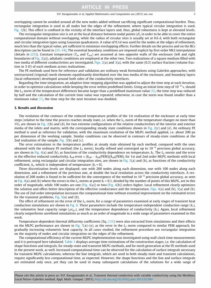
The error estimations in the temperature profiles at steady state obtained by each method, compared with the onesobtained with the ordinary FE method (the L2 norm), locally refined and converged up to 10�6 precision global accuracy,are shown in Fig. 4(a) and (b), as functions of the conductivity dependence on temperature, br. The L2 norms and the errorin the effective reduced conductivity, keff error � |keff � keff(FEM)|/keff(FEM), for 1st and 2nd order MLPG methods with localrefinement, using rectangular and circular integration sites, are shown in Fig. 5(a) and (b), as functions of the conductivitycoefficient, kr, which is independent of temperature (br = 0).

Three discretization levels are displayed; one with 200 nodes along each dimension, one with 100 nodes along eachdimension, and a refinement of the previous one, at double the local resolution across the conductivity interfaces. A res-olution of 200 nodes is found to be sufficient for the convergence of the method to 10�6 precision global accuracy, as seenin Fig. 4(a) and (b) where the errors in the L2 norms at point br = 0.1, divided by the number of points of this MLPG, are in thisorder of magnitude, while 100 nodes are one (Fig. 4(a)) or two (Fig. 4(b)) orders higher. Local refinement clearly optimizesthe solution and offers better description of the effective conductance and the temperature, Figs. 4(a) and (b), 5(a) and (b).The use of 2nd order interpolation increases the computational time without essential improvement on the estimated errorsfor the transient problems, Fig. 5(a) and (b).

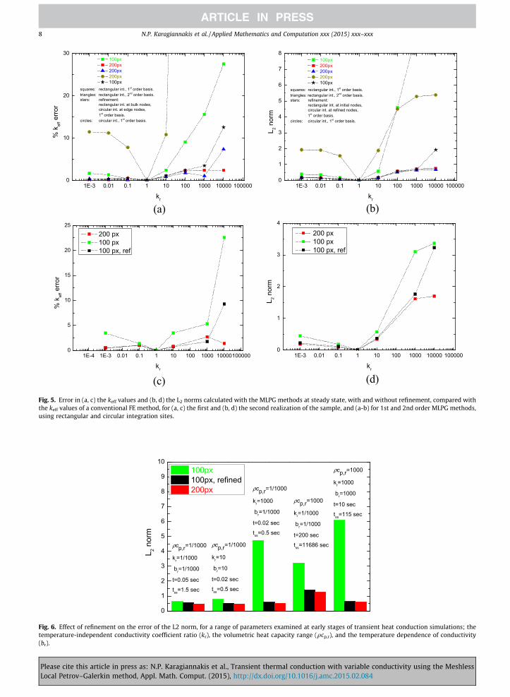
The effect of refinement on the error of the L2 norm, for a range of parameters examined at early stages of transient heatconduction simulations are shown in Fig. 6. These parameters include the temperature-independent conduction range (kr),the volumetric heat capacity range (qcp,r), and the temperature dependence of conductivity (br). Again, local refinementclearly outperforms unrefined simulations as much as an order of magnitude in a wide range of parameters examined in thiswork.

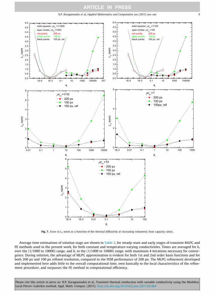
Temperature-dependent thermal diffusivity coefficients (Eq. (13)) were also extracted from simulations and their effectson the MLPG performance are shown in Fig. 7(a)–(e), as the error in the L2 norm compared to similar FEM approach, forgradually increasing volumetric heat capacity. In all cases studied, the refinement procedure use rectangular integrationon the majority of nodes and circular integration on the edges of the refinement.

The computational efficiency of the current MLPG implementation was investigated using wall-clock time measurementsand it is portrayed here tabulated. Table 1 displays average time estimations of the construction stages, i.e. the calculation ofshape functions and integrals, for steady-state and transient MLPG methods, and for mesh generation at the FE methods usedin the present work, as well. Increased computational time can be observed for the calculation of surface integrals necessaryfor transient MLPG calculations, whereas the line integrals, which are used in both steady-state and transient calculations,require significantly less computational time, as expected. However, the shape functions and the line and surface integralsare estimated only once, yet they can be used in many subsequent calculations of the solutions for a wide range of



(a)

kr=1000 ρcp,r=1/1000 t/tss=2.5‰ tss=5.57

FEM 200px / MLPG 200px / MLPG 100px ref / MLPG 100px

(b)

FEM ~200px / MLPG 200px / MLPG 100px ref / MLPG 100px

kr=1000 ρcp,r=1/1000 t=tss=5.57

(c)

kr=1/1000 ρcp,r=1000 t/tss=2.5‰ tss=45043


(d)

kr=1/1000 ρcp,r=1000 t=tss=45043


(e)

Fig. 2. (a) 1st realization of a square enclosure with varying conductivity. White regions: medium with conductivity k1 (exterior). Shaded regions: mediumwith conductivity k2 (interior). Contours of the temperature profiles using MLPG and FE methods on a square enclosure with varying conductivity (b, d) atearly time steps, and (c, e) at steady state. Conductivity of exterior medium is 1000 times (b, c) smaller or (d, e) larger than that of interior medium. Blacklines: FEM solution with �200 � 200 resolution. Red lines: MLPG, 200 � 200. Green lines: MLPG, 100 � 100. Blue lines: MLPG, 100 � 100 with localrefinement. (For interpretation of the references to color in this figure legend, the reader is referred to the web version of this article.)


parameters, like the kr and br coefficients. Compared to the FEM �200 px method, the construction phase of the MLPGapproach is comparatively faster (about 1/3 for 1st order MLPG basis function) for 100 px resolution, but slower (about3/2 for 1st order basis function, and inasmuch as 4 times for 2nd order) for 200 px resolution. However it is comparableand somewhat faster during implementation of refinement at 100 px.



(a)

kr=1000

FEM ~200px | MLPG-200px | MLPG-100px,ref | MLPG-100px

(b)

FEM ~200px | MLPG-200px | MLPG-100px,ref | MLPG-100px

kr=1/1000

(c)

Fig. 3. (a) 2nd realization of a square enclosure with varying conductivity. White regions: medium with conductivity k1 (exterior). Shaded regions: mediumwith conductivity k2 (interior). (b, c) Contours of the temperature profiles using MLPG and FE methods on a square enclosure with varying conductivity atsteady state Black lines: FEM solution with �200 � 200 resolution. Red lines: MLPG, 200 � 200. Green lines: MLPG, 100 � 100. Blue lines: MLPG, 100 � 100with local refinement. (For interpretation of the references to color in this figure legend, the reader is referred to the web version of this article.)

1E-4 1E-3 0.01 0.1 1 10 100 1000 10000

0.1

1

10

L 2 nor

m

br

opened circles: kr=1/10closed squares: kr=10

100px 100px, refined200px

(a)

1E-4 1E-3 0.01 0.1 1 10 100 1000 10000

0.1

1

10

100

L 2 nor

m

br

opened circles: kr=1/1000closed squares: kr=1000


(b)Fig. 4. Error in the L2 norm values calculated with standard and with locally refined MLPG methods (at steady state), for (a) small and (b) large values of thetemperature-independent conductivity coefficient ratio, kr, as functions of the temperature-dependent conductivity coefficient ratio, br, as defined in Eq.(13), using rectangular integration sites.




1E-3 0.01 0.1 1 10 100 1000 10000 1000000

10

20

30

squares: rectangular int., 1st order basis.triangles: rectangular int., 2nd order basis.stars: refinement:

rectangular int. at bulk nodes, circular int. at edge nodes, 1st order basis.

circles: circular int., 1st order basis.

% k

eff e

rror

kr

100px200px200px200px

100px

(a)

1E-3 0.01 0.1 1 10 100 1000 10000 1000000

1

2

3

4

5

6

7

8

squares: rectangular int., 1st order basis.triangles: rectangular int., 2nd order basis.stars: refinement:

rectangular int. at initial nodes, circular int. at refined nodes, 1st order basis.

circles: circular int., 1st order basis.

L 2 nor

m

kr

100px200px200px200px

100px

(b)

1E-4 1E-3 0.01 0.1 1 10 100 1000 100001000000

5

10

15

20

25

% k

eff e

rror

kr

200 px 100 px 100 px, ref

(c)

1E-3 0.01 0.1 1 10 100 1000 10000 1000000

1

2

3

4

L 2 nor

m

kr

200 px 100 px 100 px, ref

(d)

Fig. 5. Error in (a, c) the keff values and (b, d) the L2 norms calculated with the MLPG methods at steady state, with and without refinement, compared withthe keff values of a conventional FE method, for (a, c) the first and (b, d) the second realization of the sample, and (a-b) for 1st and 2nd order MLPG methods,using rectangular and circular integration sites.

0

1

2

3

4

5

6

7

8

9

10ρcp,r=1000

kr=1000

br=1000

t=10 sec

tss=115 sec

ρcp,r=1000

kr=1/1000

br=1/1000

t=200 sec

tss=11686 sec

ρcp,r=1/1000

kr=1000

br=1/1000

t=0.02 sec

tss=0.5 sec

ρcp,r=1/1000

kr=10

br=10

t=0.02 sec

tss=0.5 sec

L 2 nor

m


ρcp,r=1/1000

kr=1/1000

br=1/1000

t=0.05 sec

tss=1.5 sec

Fig. 6. Effect of refinement on the error of the L2 norm, for a range of parameters examined at early stages of transient heat conduction simulations; thetemperature-independent conductivity coefficient ratio (kr), the volumetric heat capacity range (qcp,r), and the temperature dependence of conductivity(br).




1E-5 1E-3 0.1 10 1000 100000 1E70.0

0.5

1.0

1.5

2.0

2.5

3.0

3.5

4.0

4.5

5.0

5.5

6.0L 2 n

orm

ar

solid squares: ρcp,r=1/1000open circles: ρcp,r=1000red points: 200 pxgreen points: 100 pxblack points: 100 px, ref

1E-5 1E-3 0.1 10 1000 1000000.0

0.5

1.0

1.5

2.0

2.5

3.0

3.5

4.0

4.5

5.0

5.5

6.0

L 2 nor

m

ar

solid squares: ρcp,r=1/100open circles: ρcp,r=100red points: 200 pxgreen points: 100 pxblack points: 100 px, ref

0.01 0.1 1 10 100 1000 100000

1

2

3

4

5

6

L 2 nor

m

ar

ρcp,r=1/10 200 px 100 px 100 px, ref

1E-3 0.01 0.1 1 10 100 10000

2

4

6

L 2 nor

m

ar

ρcp,r=1 200 px 100 px 100px, ref

1E-4 1E-3 0.01 0.1 1 10 1000

1

2

3

4

5

6

L 2 nor

m

ar

ρcp,r=10 200 px 100 px 100 px, ref

Fig. 7. Error in L2 norm as a function of the thermal diffusivity at increasing volumetric heat capacity ratios.


Average time estimations of solution stage are shown in Table 2, for steady-state and early stages of transient MLPG andFE methods used in the present work, for both constant and temperature-varying conductivities. Times are averaged for kr

over the (1/1000 to 10000) range, and br in the (1/1000 to 10000) range, with maximum 4 iterations necessary for conver-gence. During solution, the advantage of MLPG approximation is evident for both 1st and 2nd order basis functions and forboth 200 px and 100 px refined resolution, compared to the FEM performance of 200 px. The MLPG refinement developedand implemented here adds little to the overall computational time, own basically to the local characteristics of the refine-ment procedure, and surpasses the FE method in computational efficiency.



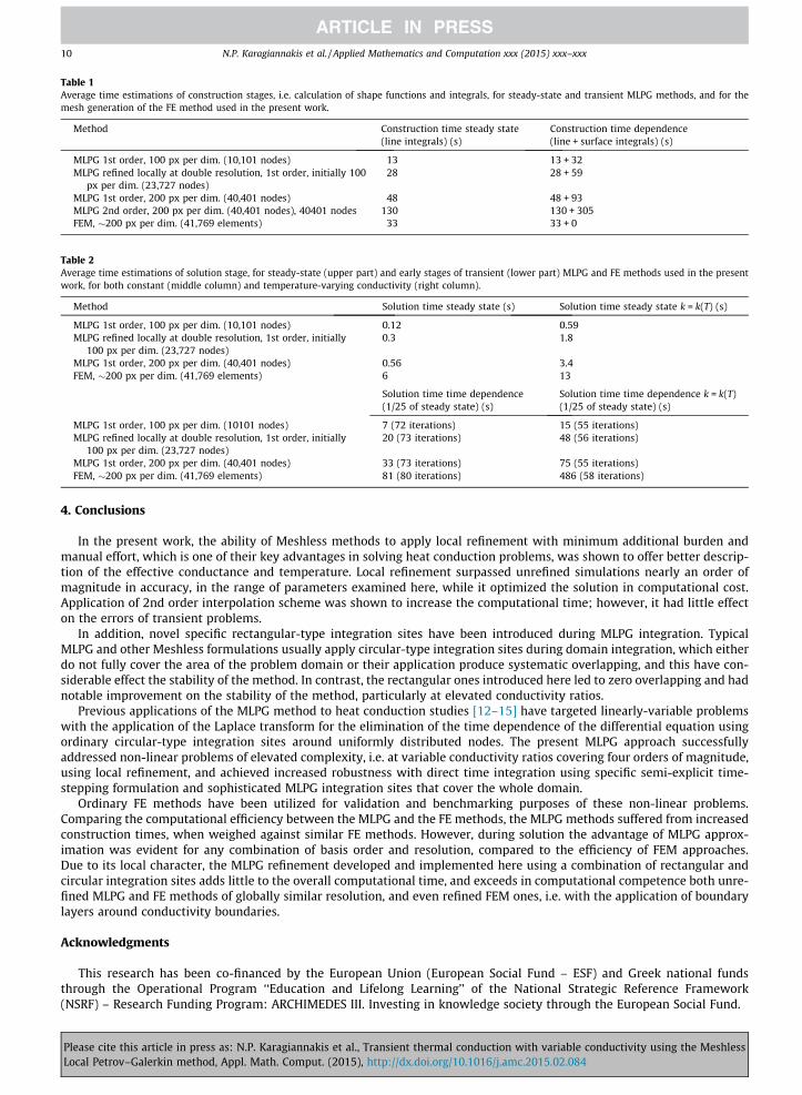
Table 1Average time estimations of construction stages, i.e. calculation of shape functions and integrals, for steady-state and transient MLPG methods, and for themesh generation of the FE method used in the present work.

Method Construction time steady state(line integrals) (s)

Construction time dependence(line + surface integrals) (s)

MLPG 1st order, 100 px per dim. (10,101 nodes) 13 13 + 32MLPG refined locally at double resolution, 1st order, initially 100

px per dim. (23,727 nodes)28 28 + 59

MLPG 1st order, 200 px per dim. (40,401 nodes) 48 48 + 93MLPG 2nd order, 200 px per dim. (40,401 nodes), 40401 nodes 130 130 + 305FEM, �200 px per dim. (41,769 elements) 33 33 + 0

Table 2Average time estimations of solution stage, for steady-state (upper part) and early stages of transient (lower part) MLPG and FE methods used in the presentwork, for both constant (middle column) and temperature-varying conductivity (right column).

Method Solution time steady state (s) Solution time steady state k = k(T) (s)

MLPG 1st order, 100 px per dim. (10,101 nodes) 0.12 0.59MLPG refined locally at double resolution, 1st order, initially

100 px per dim. (23,727 nodes)0.3 1.8

MLPG 1st order, 200 px per dim. (40,401 nodes) 0.56 3.4FEM, �200 px per dim. (41,769 elements) 6 13

Solution time time dependence(1/25 of steady state) (s)

Solution time time dependence k = k(T)(1/25 of steady state) (s)

MLPG 1st order, 100 px per dim. (10101 nodes) 7 (72 iterations) 15 (55 iterations)MLPG refined locally at double resolution, 1st order, initially

100 px per dim. (23,727 nodes)20 (73 iterations) 48 (56 iterations)

MLPG 1st order, 200 px per dim. (40,401 nodes) 33 (73 iterations) 75 (55 iterations)FEM, �200 px per dim. (41,769 elements) 81 (80 iterations) 486 (58 iterations)


4. Conclusions

In the present work, the ability of Meshless methods to apply local refinement with minimum additional burden andmanual effort, which is one of their key advantages in solving heat conduction problems, was shown to offer better descrip-tion of the effective conductance and temperature. Local refinement surpassed unrefined simulations nearly an order ofmagnitude in accuracy, in the range of parameters examined here, while it optimized the solution in computational cost.Application of 2nd order interpolation scheme was shown to increase the computational time; however, it had little effecton the errors of transient problems.

In addition, novel specific rectangular-type integration sites have been introduced during MLPG integration. TypicalMLPG and other Meshless formulations usually apply circular-type integration sites during domain integration, which eitherdo not fully cover the area of the problem domain or their application produce systematic overlapping, and this have con-siderable effect the stability of the method. In contrast, the rectangular ones introduced here led to zero overlapping and hadnotable improvement on the stability of the method, particularly at elevated conductivity ratios.

Previous applications of the MLPG method to heat conduction studies [12–15] have targeted linearly-variable problemswith the application of the Laplace transform for the elimination of the time dependence of the differential equation usingordinary circular-type integration sites around uniformly distributed nodes. The present MLPG approach successfullyaddressed non-linear problems of elevated complexity, i.e. at variable conductivity ratios covering four orders of magnitude,using local refinement, and achieved increased robustness with direct time integration using specific semi-explicit time-stepping formulation and sophisticated MLPG integration sites that cover the whole domain.

Ordinary FE methods have been utilized for validation and benchmarking purposes of these non-linear problems.Comparing the computational efficiency between the MLPG and the FE methods, the MLPG methods suffered from increasedconstruction times, when weighed against similar FE methods. However, during solution the advantage of MLPG approx-imation was evident for any combination of basis order and resolution, compared to the efficiency of FEM approaches.Due to its local character, the MLPG refinement developed and implemented here using a combination of rectangular andcircular integration sites adds little to the overall computational time, and exceeds in computational competence both unre-fined MLPG and FE methods of globally similar resolution, and even refined FEM ones, i.e. with the application of boundarylayers around conductivity boundaries.

Acknowledgments

This research has been co-financed by the European Union (European Social Fund – ESF) and Greek national fundsthrough the Operational Program ‘‘Education and Lifelong Learning’’ of the National Strategic Reference Framework(NSRF) – Research Funding Program: ARCHIMEDES III. Investing in knowledge society through the European Social Fund.




References

[1] A. Bejan, Heat Transfer, John Wiley & Sons, NY, 1993.[2] S. Mahjoob, K. Vafai, Analytical characterization of heat transport through biological media incorporating hyperthermia treatment, Int. J. Heat Mass

Transfer 52 (2009) 1608–1618.[3] T.C. Chiam, Heat transfer with variable conductivity in a stagnation-point flow towards a stretching sheet, Int. Commun. Heat Mass Transfer 23 (1996)

239–248.[4] M. Arunachalam, N.R. Rajappa, Thermal-boundary layer in liquid-metals with variable thermal-conductivity, Appl. Sci. Res. 34 (1978) 179–187.[5] G.E. Wnek, J.C.W. Chien, F.E. Karasz, M.A. Druy, Y.W. Park, A.G. MacDiarmid, A.J. Heeger, Variable-density conducting polymers: conductivity and

thermopower studies of a new form of polyacetylene: (CH)x, J. Polym. Sci. Polym. Lett. Edition 17 (1979) 779–786.[6] B. Nayroles, G. Touzot, P. Villon, Generalizing the finite element method: diffuse approximation and diffuse elements, Comput. Mech. 10 (1992) 307–

318.[7] T. Belytschko, Y.Y. Lu, L. Gu, Element-free Galerkin methods, Int. J. Numer. Methods Eng. 37 (1994) 229–256.[8] D. Organ, M. Fleming, T. Terry, T. Belytschko, Continuous meshless approximations for nonconvex bodies by diffraction and transparency, Comput.

Mech. 18 (1996) 225–235.[9] T. Zhu, S.N. Atluri, A modified collocation method and a penalty formulation for enforcing the essential boundary conditions in the element free

Galerkin method, Comput. Mech. 21 (1998) 211–222.[10] W.K. Liu, Y. Chen, C.T. Chang, T. Belytschko, Advances in multiple scale kernel particle methods, Comput. Mech. 18 (1996) 73–111.[11] G.C. Bourantas, E.D. Skouras, V.C. Loukopoulos, G.C. Nikiforidis, An accurate, stable and efficient domain-type meshless method for the solution of MHD

flow problems, J. Comput. Phys. 228 (2009) 8135–8160.[12] J. Sladek, V. Sladek, C. Zhang, Transient heat conduction analysis in functionally graded materials by the meshless local boundary integral equation

method, Comput. Mater. Sci. 28 (2003) 494–504.[13] V. Sladek, J. Sladek, M. Tanaka, C. Zhang, Transient heat conduction in anisotropic and functionally graded media by local integral equations, Eng. Anal.

Bound. Elem. 29 (2005) 1047–1065.[14] J. Sladek, V. Sladek, C. Hellmich, J. Eberhardsteiner, Heat conduction analysis of 3-D axisymmetric and anisotropic FGM bodies by meshless local

Petrov–Galerkin method, Comput. Mech. 39 (2007) 323–333.[15] J. Sladek, V. Sladek, C.L. Tan, S.N. Atluri, Analysis of transient heat conduction in 3D anisotropic functionally graded solids, by the MLPG method, CMES

– Comput. Model. Eng. Sci. 32 (2008) 161–174.[16] S.N. Atluri, T. Zhu, A new meshless local Petrov–Galerkin (MLPG) approach in computational mechanics, Comput. Mech. 22 (1998) 117–127.[17] G.C. Bourantas, E.D. Skouras, G.C. Nikiforidis, Adaptive support domain implementation on the moving least squares approximation for mfree methods

applied on elliptic and parabolic pde problems using strong-form description, CMES – Comput. Model. Eng. Sci. 43 (2009) 1–25.[18] A.N. Kalarakis, G.C. Bourantas, E.D. Skouras, V.C. Loukopoulos, V.N. Burganos, Lattice-Boltzmann and meshless point collocation solvers for fluid flow

and conjugate heat transfer, Int. J. Numer. Methods Fluids 70 (2012) 1428–1442.[19] G.C. Bourantas, A.J. Petsi, E.D. Skouras, V.N. Burganos, Meshless point collocation for the numerical solution of Navier–Stokes flow equations inside an

evaporating sessile droplet, Eng. Anal. Bound. Elem. 36 (2012) 240–247.[20] G.C. Bourantas, E.D. Skouras, V.C. Loukopoulos, V.N. Burganos, Heat transfer and natural convection of nanofluids in porous media, Eur. J. Mech. B Fluids

43 (2014) 45–56.[21] E.D. Skouras, G.C. Bourantas, V.C. Loukopoulos, G.C. Nikiforidis, Truly meshless localized type techniques for the steady-state heat conduction

problems for isotropic and functionally graded materials, Eng. Anal. Bound. Elem. 35 (2011) 452–464.[22] N. Karagiannakis, G.C. Bourantas, A.N. Kalarakis, E.D. Skouras, V.N. Burganos, Efficiency of the meshless local Petrov–Galerkin method with moving

least squares approximation for thermal conduction applications, in: T. Simos (Ed.) ICNAAM 2013, Rhodos, Greece, 2013.[23] S.N. Atluri, Z.D. Han, A.M. Rajendran, A new implementation of the meshless finite volume method, through the MLPG ‘‘Mixed’’ approach, CMES –

Comput. Model. Eng. Sci. 6 (2004) 491–513.[24] X.H. Wu, W.Q. Tao, Meshless method based on the local weak-forms for steady-state heat conduction problems, Int. J. Heat Mass Transf. 51 (2008)

3103–3112.


http://refhub.elsevier.com/S0096-3003(15)00284-2/h0005











































Transient thermal conduction with variable conductivity ...€¦ · A numerical solution of the...

Documents

Transcript of Transient thermal conduction with variable conductivity ...€¦ · A numerical solution of the...