Transient Simulation of a Sub- to Transcritical C0 ...

Transient Simulation of a Sub- to Transcritical

C02 Refrigeration Cycle

by

Michael Garces de Gois

Thesispresented in partial fulfilment of the requirements for the degree

of Master of Engineering (lvfechanical ) in the Faculty of Engineering at

Stellenbosch University

Supervisor: Mr Robert T. Dobson

March 2016

i

DECLARATION

By submitting this thesis electronically, I declare that the entirety of the work

contained therein is my own, original work, that I am the sole author thereof (save

to the extent explicitly otherwise stated), that reproduction and publication thereof

by Stellenbosch University will not infringe any third party rights and that I have

not previously in its entirety or in part submitted it for obtaining any qualification.

Date: ……………………………………….

Copyright © 2016 Stellenbosch University

All rights reserved

Stellenbosch University https://scholar.sun.ac.za

ii

ABSTRACT

The purpose of this project is to develop a numerical transient simulation model

of the CO2 refrigeration cycle containing a capillary tube as expansion device. A

design procedure for CO2 refrigerators is also developed; which makes use of a

steady-state capillary tube model for acquiring the initial design of the capillary

tube, and uses the transient simulation program to determine the low pressure

side internal volume and validate the complete design of the refrigerator. Using

this design procedure a CO2 refrigerator was designed, built and then tested to

validate the simulation model developed. The project was conducted at the

Department of Mechanical and Mechatronic Engineering at the University of

Stellenbosch.

A literature review on the history of refrigeration, the vapour-compression

refrigeration cycle, the transcritical CO2 refrigeration cycle, refrigerant properties,

CO2 properties, and a comparison of refrigerant performance was done as

background to the use of CO2 as refrigerant. Furthermore, literature review of an

alternative expansion device, the vortex tube, was included, but found not

practical for implementing with CO2 which behaves more like a real gas and not

an ideal gas. Lastly, theory on the development of the one-dimensional CFD

finite volume method in terms of a general variable is shown. This provides

background to the development of discretised conservation equations for the

simulation model.

The transient model developed is capable of predicting transient operation from

stand-still starting conditions through to steady-state conditions. The model

makes use of well-known pipe friction and heat transfer correlations.

Furthermore, it makes use of the real gas equation of state for CO2 from Span

and Wagner (1996). Moreover, the model determines whether the flow is single -

or two-phase and then calculates the appropriate properties. Lastly, it has the

whole refrigerant circuit, from compressor outlet back to compressor inlet, as the

simulation domain.

The simulation results for the pressure and temperature distributions show the

transient behaviour at start-up. The transient and steady-state results also agree

fairly well with the experimental results. The steady-state pressure graphs are as

expected and the constant evaporation temperature is a confirmation that the

model approximates real life operation quite well. In conclusion, the results show

that the simulation model is a useful tool for designing and understanding

capillary tube CO2 refrigeration cycles. Future work involves developing a non-

adiabatic compressor model and models for alternative expansion devices to be

included in the current refrigerator simulation model.


iii

OPSOMMING

Die doel van hierdie projek is om ’n numeriese oorgangsfase-simulasie-model

van ŉ CO2 verkoelingstelsel met ’n haarbuis as uitbreidingstoestel te ontwikkel.

’n Ontwerp prosedure vir CO2 yskaste word ook ontwikkel; wat gebruik maak van

ŉ bestendige toestand haarbuis model vir die verkryging van die aanvanklike

ontwerp van die haarbuis, en maak gebruik van die oorgangsfase-simulasie

program om die lae druk kant se interne volume te bepaal en die geldigheid van

die volledige ontwerp van die yskas te bevestig. Deur die toepassing van hierdie

ontwerp prosedure is ŉ CO2 yskas ontwerp, gebou en dan getoets om die

simulasie program wat ontwikkel is te valideer. Die projek is voltooi by die

Departement van Meganiese en Megatroniese Ingenieurswese aan die

Universiteit van Stellenbosch.

’n Literatuuroorsig oor die geskiedenis van verkoeling, die damp-samedrukkings

verkoelingsiklus, die transkritiese CO2 verkoelingsiklus, koelmiddel eienskappe,

CO2 eienskappe, en ’n vergelyking van koelmiddel prestasie is gedoen as

agtergrond vir die gebruik van CO2 as koelmiddel. Verder is ’n literatuuroorsig

van ’n alternatiewe uitbreidingstoestel, die vortex buis, ingesluit, maar daar is

gevind dat hierdie toestel nie praktiese is vir die implementering met CO2 nie;

omdat CO2 eerder as ŉ werklike en nie ŉ ideale gas optree nie. Laastens word

die teorie oor die ontwikkeling van die een-dimensionele numeriese

vloeidinamika eindige volume metode in terme van ’n algemene veranderlike

getoon. Dit bied agtergrond tot die ontwikkeling van die gediskritiseerde

behoudsvergelykings vir die simulasie model.

Die ontwikkelde oorgangsfase-model is in staat om die oorgangsfase te voorspel

van die rustende begintoestand tot by die bestendigetoestand. Die model maak

gebruik van bekende pyp wrywing en hitte-oordrag korrelasies. Verder, maak dit

gebruik van die werklike gas toestandsvergelyking vir CO2 van Span en Wagner

(1996). Nog verder, bepaal die model of die vloei enkel- of twee-fase is, en

bereken dan die geskikte eienskappe. Laastens, dit het as die simulasie domein

die hele koelmiddel kringloop vanaf die kompressor uitlaat terug na die

kompressor inlaat.

Die simulasie resultate vir die druk- en temperatuurverspreidings wys die gedrag

van die oorgangsfase vanaf begin toestand. Die oorgangsfase en

bestendigetoestand resultate stem redelik goed ooreen met die eksperimentele

resultate. Die bestendigetoestand drukgrafieke is soos verwag, en die konstante

verdampingstemperatuur is ’n bevestiging dat die model werklike werking baie

goed benader.

Ten slotte, die resultate toon dat die simulasie model ŉ nuttige instrument is vir

die ontwerp en begrip van haarbuis CO2 verkoelingsiklusse. Toekomstige werk


iv

behels die ontwikkeling van ’n nie-adiabatiese kompressor model en simulasie

modelle vir alternatiewe uitbreidings toestelle wat in die huidige yskas-simulasie

model geïmplementeer kan word.


v

ACKNOWLEDGEMENTS

I would like to thank my supervisor, Mr R.T. Dobson, for his guidance, patience

and effort in helping me in this project. Also, I would like to thank GDK

Installations for charging my refrigeration system with CO2. Furthermore, I

express my gratitude to all the mechanical workshop staff, including Mr F.

Zietsman and Mr C. Zietsman, for their assistance and advice. I especially thank

my friends and family for their continual support and encouragement.


vi

TABLE OF CONTENTS

LIST OF FIGURES.............................................................................................. x

LIST OF TABLES ............................................................................................. xii

NOMENCLATURE ........................................................................................... xiii

1. INTRODUCTION .......................................................................................... 1

1.1. Objectives .......................................................................................... 2

1.2. Motivation .......................................................................................... 3

2. LITERATURE REVIEW AND THEORY ....................................................... 4

2.1. The History of Refrigeration ............................................................... 4

2.2. Theoretical Vapour-Compression Refrigeration Cycle ........................ 6

2.3. Carbon Dioxide (CO2) Transcritical Refrigeration Cycle ..................... 7

2.4. Refrigerant Properties ........................................................................ 7

2.4.1. Ideal Properties of a Refrigerant ........................................... 8

2.4.2. Properties of Carbon Dioxide................................................ 8

2.4.3. Refrigerant Comparison ....................................................... 9

2.5. The Vortex Tube as an Alternative Expansion Device ...................... 11

2.5.1. Experimental Studies ......................................................... 11

2.5.2. Analytical and Numerical Studies ....................................... 13

2.5.3. Geometrical Properties of the Vortex Tube ......................... 13

2.5.4. Thermo-Physical Parameters ............................................. 17

2.6. The Finite Volume Method ............................................................... 17

3. DETERMINING THE THERMODYNAMIC STATE ..................................... 23

3.1. CO2 Equation of State from Span and Wagner ................................ 23

3.2. Saturated Property Determination .................................................... 25

3.3. Determining Single Phase and Two-Phase Properties ..................... 26

3.3.1. Determining Single Phase Properties ................................. 27

3.3.2. Determining Two-Phase Properties .................................... 28

3.3.3. Deciding whether the Fluid is Single Phase or Two-Phase . 31

4. TRANSIENT SIMULATION PROGRAM OF THE CO2 REFRIGERATION

CYCLE .............................................................................................................. 33


vii

4.1. General Model Assumptions ............................................................ 33

4.2. Initialising the Simulation Domain .................................................... 33

4.2.1. Defining Geometric Properties of the Simulation Domain ... 33

4.2.2. Initial Conditions for the Simulation Domain ....................... 35

4.3. Boundary Conditions for the Simulation Domain .............................. 36

4.4. Updating to the New Time-Step ....................................................... 38

4.5. Heat Transfer and Friction Definitions .............................................. 38

4.6. Determining the Properties of Water ................................................ 41

4.7. Discretisation of Equations of Change Applied to Control Volumes .. 42

4.7.1. Discretisation of the Conservation of Mass ......................... 43

4.7.2. Discretisation of the Conservation of Energy ...................... 44

4.7.3. Discretisation of the Conservation of Momentum................ 45

4.8. Algorithm for Simulating a Refrigeration Cycle ................................. 46

5. REFRIGERATOR DESIGN ........................................................................ 49

5.1. Compressor Selection ...................................................................... 49

5.2. Internal Volume of High Pressure Side ............................................ 49

5.3. Capillary Tube Design using a Steady-State Capillary Tube Simulation

Model ........................................................................................ 51

5.4. Internal Volume of Low Pressure Side ............................................. 53

5.5. Heat Exchanger Designs ................................................................. 54

5.6. Final Design of Refrigerator ............................................................. 55

6. EXPERIMENTAL SETUP .......................................................................... 56

6.1. Thermocouple Calibration ................................................................ 56

6.2. Experimental System Layout ........................................................... 57

6.3. Experimental Procedure................................................................... 58

7. SIMULATION SETUP ................................................................................ 60

7.1. Initial State of the Simulation Domain............................................... 60

7.2. Boundary Conditions and External Heat Exchangers ....................... 61

7.3. Grid Independence .......................................................................... 61

7.4. Simulation Domain Geometry Properties ......................................... 62

8. SIMULATION RESULTS ........................................................................... 63

8.1. Transient Simulation Results ........................................................... 63


viii

8.2. Steady-State Results ....................................................................... 69

9. EXPERIMENTAL VERSUS SIMULATION RESULTS ............................... 71

10. OTHER EXPERIMENTAL RESULTS ........................................................ 76

11. DISCUSSION OF RESULTS ..................................................................... 77

12. CONCLUSIONS AND RECOMMENDATIONS FOR FUTURE WORK ...... 79

13. REFERENCES........................................................................................... 81

APPENDIX A: SAMPLE CALCULATIONS ..................................................... 84

A1: Sample Calculations for an Ideal CO2 Refrigeration Cycle with an

Ideal Work Recovering Expansion Device ................................ 84

APPENDIX B: Property Function Codes for CO2 .......................................... 87

B1: Function to Calculate the Single Phase Properties at a Given Density

and Temperature ...................................................................... 87

B2: Function to Calculate the Saturated Properties at a Given

Temperature ............................................................................. 90

B3: Function to Calculate the Single Phase Properties at a Given Density

and Specific Internal Energy ..................................................... 91

B4: Derivatives Used in the Formulation of the Two-Phase Function ..... 91

B5: Function to Calculate the Two-Phase Properties at a Given Density

and Specific Internal Energy ..................................................... 93

B6: Function to Calculate the Thermal Conductivity ............................... 95

B7: Function to Calculate the Dynamic Viscosity .................................... 95

B8: Function to Calculate the Properties at a Given Density and Specific

Internal Energy ......................................................................... 96

APPENDIX C: TRANSIENT SIMULATION PROGRAM................................... 97

C1: Main Program Code of the Transient Simulation Model ................... 97

C2: Program Code to Assign Initial Conditions of the Simulation Model . 98

C3: Program Code to Update Variables for the New Time-Step ........... 106

C4: Program Code to Solve the Three Conservation Equations ........... 106

APPENDIX D: COMPRESSOR PRODUCT DATA ........................................ 117

APPENDIX E: STEADY-STATE CAPILLARY TUBE SIMULATION MODEL 118

APPENDIX F: THERMOCOUPLE CALIBRATION ........................................ 121


ix

APPENDIX G: EXPERIMENTAL APPARATUS ............................................ 122

G1: Embraco EK6210CD Compressor ................................................. 122

G2: Pressure Gauges ........................................................................... 122

G3: B.I.C.I.SA-5500 Water Pump ......................................................... 123

G4: Hailea HS-28A Water Chiller .......................................................... 124

G5: Agilent 34970A Data Acquisition/Data Logger Switch Unit ............. 125

G6: Efergy Energy Monitoring Socket ................................................... 126


x

LIST OF FIGURES

Figure 1: Vapour-compression refrigeration cycle .............................................. 6

Figure 2: CO2 refrigeration cycle ........................................................................ 7

Figure 3: Ideal CO2 refrigeration cycle operating at 258 K and 303 K ................. 9

Figure 4: Counter-flow vortex tube ................................................................... 11

Figure 5: Tangential inlet nozzles ..................................................................... 15

Figure 6: Control volume for tube fluid flow ...................................................... 18

Figure 7: Notation used in the control volume discretisation ............................. 19

Figure 8: Phase diagram for CO2 ..................................................................... 31

Figure 9: Program logic to determine the properties of CO2 at a given density

and specific internal energy ............................................................................... 32

Figure 10: Basic refrigeration cycle for simulation ............................................ 34

Figure 11: Tube-in-tube thermal resistance diagram ........................................ 38

Figure 12: Control volume description .............................................................. 42

Figure 13: Density-based algorithm for solving compressible flow .................... 48

Figure 14: Steady-state capillary tube model .................................................... 51

Figure 15: Refrigerator final design .................................................................. 55

Figure 16: Thermocouple 1 - calibration curve .................................................. 57

Figure 17: Experimental system ....................................................................... 57

Figure 18: Compressor control unit (left) and measuring equipment (right) ...... 58

Figure 19: Initial state of the simulation domain: (a) temperature, (b) pressure,

(c) density, (d) vapour quality ............................................................................ 60

Figure 20: Pressure distribution at 150 ms for grid independence study ........... 61

Figure 21: Control volume length distribution.................................................... 63

Figure 22: Transient pressure development ..................................................... 64

Figure 23: Transient temperature development ................................................ 65

Figure 24: Transient velocity development ....................................................... 66

Figure 25: Transient mass flow rate development of: (a) simulation domain, (b)

compressor ....................................................................................................... 67

Figure 26: Transient development of: (a) evaporator heat absorption rate, (b) gas

cooler heat rejection rate ................................................................................... 67

Figure 27: Transient vapour quality development ............................................. 68

Figure 28: Steady-state results for the distribution of: (a) pressure, (b)

temperature, (c) velocity, (d) vapour quality ....................................................... 69


xi

Figure 29: Steady-state pressure drop for: (a) HP side, (b) capillary tube, (c) LP

side ................................................................................................................... 70

Figure 30: Comparison of pressure development ............................................. 72

Figure 31: Comparison of compressor inlet and outlet temperature .................. 72

Figure 32: Comparison of evaporator (a) inlet temperature, (b) cooling load .... 73

Figure 33: Comparison of gas cooler cooling section (a) steady-state

temperature distribution, (b) heat transfer rate................................................... 73

Figure D1: EK6210CD product data ............................................................... 117

Figure G1: Embraco EK6210CD Compressor ................................................ 122

Figure G2: Swagelok pressure gauges ........................................................... 123

Figure G3: B.I.C.I.SA-5500 water pump ......................................................... 123

Figure G4: Hailea HS-28A water chiller .......................................................... 124

Figure G5: Agilent 34970A Data Acquisition/Switch Unit ................................ 125

Figure G6: Efergy energy monitoring socket .................................................. 126


xii

LIST OF TABLES

Table 1: Comparative refrigerant performance per kilowatt of refrigeration ....... 10

Table 2: Work recovering device versus normal throttling device ..................... 10

Table 3: Relations of the thermodynamic properties to the dimensionless

Helmholtz function ......................................................................................... 24

Table 4: Tube details of the high pressure side ................................................ 50

Table 5: Tube details of the low pressure side .................................................. 53

Table 6: Details of the outer tubes of the heat exchangers ............................... 54

Table 7: Comparison of experimental and simulation results ............................ 74

Table 8: Steady-state experimental results for different water inlet temperatures

.......................................................................................................................... 76

Table F1: Thermocouple calibration equations ............................................... 121


xiii

NOMENCLATURE

Cross-sectional area [m2]

Specific Helmholtz energy [kJ/k ]

Inlet area of the first control volume [m2]

Coefficient variable

Skin friction factor

Speed of sound [m/s]

Specific heat capacity at constant pressure [kJ/(k K)]

Specific heat capacity at constant volume [kJ/(k K)]

Diameter [m]

Hydraulic diameter [m]

Inner diameter [m]

Outer diameter [m]

Convection variable

Function; Vector of function values; Length ratio variable

Specific Gibbs energy [kJ/k ]

Specific enthalpy [kJ/k ]

Heat transfer coefficient [W/(m2 K)]

Matrix of derivatives

Loop variable for control volumes [-]

Conductivity [W/(m K)]

Length [m]

Mass [k ]


xiv

Mass flow rate [k /s]

Number of variables/control volumes [-]

Compressor speed [rpm]

Nusselt number [-]

Pressure [kPa]

Vapour/saturation pressure [kPa]

Prandtl number [-]

Heat transfer rate [W]

Specific gas constant [kJ/(k K)]

Thermal resistance [K/W]

Reynolds number [-]

Radial direction/length [m]; Stretch ratio [-]

Source term

Constant part of source term

Part of source term that depends on the variable value

Entropy [kJ/(k K)]

Temperature [K]

Time [s]; Coefficient variable

Specific internal energy [kJ/k ]

Given specific internal energy [kJ/k ]

Volume [m3]

Displacement volume of the compressor [m3]

Volume of the system [m3]


xv

Velocity [m/s]

Vector of unknowns

Axial direction/length [m]

Greek

Void fraction [-]

Relaxation factor for velocity [-]

Pressure drop [kPa]

Time step size [s]

Infinitesimal volume [m3]

Infinitesimal axial length [m]

Reduced density [-]

Isentropic efficiency [-]

Volumetric efficiency [-]

Fluid dynamic viscosity [Pa s]

Perimeter [m]

General variable; Dimensionless Helmholtz energy [-]

Density [k /m3]

Given density [k /m3]

Inverse reduced temperature [-]

Shear stress due to wall friction [Pa]

-direction/angle [rad]

Specific volume [m3/k ]


xvi

Subscripts

Carbon dioxide

Copper

Critical point value

Compressor

Capillary tube

Property at the capillary tube inlet

Single phase region of the capillary tube

Two-phase region of the capillary tube

Connecting tube between compressor and gas cooler

Environmental condition

East face

Evaporator

Connecting tube between evaporator and internal heat

exchanger

Saturated liquid value

Saturated vapour value

Gas cooler

Connecting tube between gas cooler and internal heat

exchanger

Internal heat exchanger

Connecting tube between internal heat exchanger and

compressor


xvii

Connecting tube between internal heat exchanger and

capillary tube

’th iteration; Inner tube/fluid

Inlet condition of the simulation domain

Property at the inlet of the evaporator

Inlet condition of the compressor

Outer tube/fluid

Outlet condition of the simulation domain

Property at the outlet of the evaporator

Outlet condition of the compressor

Isentropic outlet condition of the compressor

Node P; At constant pressure

Total

Specific internal energy

West face

z-direction

General variable

Superscripts

Exponent

Old value; Ideal-gas part of dimensionless Helmholtz

energy

Residual part of dimensionless Helmholtz energy

Value at time t


xviii

Time step

(over bar) Average value

Guess value

Abbreviations/Acronyms

CFC Chlorofluorocarbon

CFD Computational fluid dynamics

COP Coefficient of performance

CO2 Carbon dioxide

CV Control volume

E East node

GC Gas cooler

GWP Global warming potential

HP High pressure side

LP Low pressure side

ODP Ozone depletion potential

O2 Oxygen

P Node P

TDMA Tri-diagonal matrix algorithm

W West node

1-D One-dimensional


1

1. INTRODUCTION

Refrigeration has become a highly essential part of modern day living; it is used

to preserve food, cool drinks, maintain a comfortable environment through air

conditioning, and to preserve organs for transplants in hospitals amongst other

uses. Refrigeration comes in various forms, ranging from large to small

refrigeration systems for use in supermarkets and households, respectively.

According to Barthel and Götz (2012: 3) in 2012, an estimated 1.4 billion

refrigerators and freezers were in use worldwide, with an average annual

electricity consumption of 450 kWh each; this amounts to a staggering total

annual consumption of 649 TWh.

The first refrigerators in the 1800’s used refrigerants such as sulphur dioxide,

ether, methyl chloride, carbon dioxide (CO2), as well as vinegar, wine, brandy,

etc. (Briley, 2004). These systems were quite inefficient at first, but as time went

on more knowledge of refrigerator construction methods and what properties the

ideal refrigerant should exhibit became known. This led to the development of

synthetic refrigerants such as Chlorofluorocarbons (CFC’s). It was later

discovered that these synthetic refrigerants cause ozone depletion and are partly

responsible for global warming. Subsequently, their use was being phased out

by the Montreal Protocol (1987), thus triggering renewed interest in designing

refrigeration systems that work with safe alternative natural gases, such as CO2.

Improving refrigeration cycles has been the topic of many recent research

papers, specifically CO2 transcritical cycles (Sarkar, 2009). The cycle is called

transcritical since it typically operates with the low pressure side at subcritical

pressures and the high pressure side at supercritical pressures. The high

pressure difference between these two sides causes a high irreversible friction

loss when conventional expansion devices, such as capillary tube or expansion

valve, are used. The urge to design and manufacture CO2 refrigeration cycles

with a higher COP has led to the development of simulation models to obtain a

better understanding of the cycle’s operating characteristics; to ascertain whether

the high expansion loss through these expansion devices relates to the lower

COP, and also to identify areas for improvement. The simulation models are also

used to cut down on system design time and costs. It is of interest to see how

the refrigeration cycle reaches steady state operation from standstill initial

conditions. This has inspired the development of a transient simulation model of

a system containing a capillary tube, capable of transient start-up from standstill

subcritical conditions through to transcritical operation. The program uses a one-

dimensional computational fluid dynamics (1D-CFD) finite volume approach and

has the whole refrigeration circuit, from compressor outlet back to compressor

inlet, as the simulation domain.


2

This project presents an investigation into the literature of vapour-compression

refrigeration cycles, CO2 transcritical refrigeration cycles, and CO2 properties;

with the purpose of developing a transient simulation model of a CO2 refrigerator

and then constructing a CO2 refrigerator capable of being used to validate the

model. The project was proposed and supervised by Mr R.T. Dobson. This

report discusses the objectives and motivation for the project, the literature

review as background to the project, as well as literature on an alternative

expansion device (the vortex tube) to investigate the possibility of increasing the

COP of the refrigeration cycle. Also, it focuses on the use of the real gas

equation of state from Span and Wagner (1996) to determine the thermodynamic

properties of CO2 for the control volume method. Furthermore, it discusses the

development of the transient numerical simulation model capable of both single -

and two-phase flow, the design and manufacture of a CO2 refrigerator, the

simulation and experimental results obtained, as well as a discussion of the

results, conclusions and recommendations for future work.

1.1. Objectives

This project is aimed at developing a sub- to transcritical transient numerical

simulation model of a CO2 refrigeration cycle containing a capillary tube as

expansion device. A literature review of refrigeration cycles and CO2 properties

was deemed necessary in providing the background to design and construct a

CO2 refrigeration system which can be used to experimentally validate the

simulation’s results. The objectives of the project are therefore:

Perform a literature review of refrigeration cycles and CO2 transcritical

cycles.

Investigate the properties of CO2 in view of using it as refrigerant.

Introduce literature of an alternative expansion device, the vortex tube, to

investigate whether it can be used to increase the cycle’s efficiency.

Conduct a literature study on the control volume method, with the view to

implementing it into the numerical simulation model.

Describe the use of the real gas equation of state from Span and

Wagner (1996) to determine the properties of CO2 in a control volume,

whether it’s single - or two-phase.

Develop discretised forms of the conservation equations and thus

describe the development of the 1-D CFD finite volume transient

simulation model of the refrigeration system.

Construct a CO2 refrigeration system with tube-in-tube external heat

exchangers for the evaporator and gas-cooler. Water will be used in the

outer tube since it allows for accurate measurement of heat addition or

removal, also it allows for easier control of operating conditions for the

refrigeration system.

Perform experimental testing of the CO2 refrigeration cycle built.


3

Compare experimental and simulation results to validate the simulation

model.

1.2. Motivation

Carbon dioxide, a by-product of all living breathing creatures, is part of the earth’s

natural atmospheric cycle. It is expelled by living creatures and by burning fossil

fuels, absorbed by trees and plants during photosynthesis to again produce clean

oxygen (O2). Carbon dioxide has a zero ozone depletion potential, a low global

warming potential, is non-toxic, non-flammable, and along with other

thermodynamic properties, such as high volumetric refrigerating capacity, greatly

reduced compression ratio and high heat transfer properties, makes it a very

attractive natural gas to use as refrigerant (Sarkar, 2010). The high pressures

needed for heat rejection during operation has been the limiting factor in the past

and hence its abandonment as a refrigerant. The higher pressure differential

causes higher velocities in the expansion devices and thus higher irreversible

friction losses through capillary tubes/expansion valves; thereby, leaving these

CO2 cycles with an inferior COP when compared to similar cycles using synthetic

refrigerants.

A simulation model of the CO2 refrigeration cycle may provide valuable

information relating to its performance characteristics. Numerically simulating

components of a refrigeration cycle, and then combining these single component

results to have a complete solution for the refrigeration cycle, is what many

researchers have done, such as Jensen (2008), Susort (2012), and Zhang et al.

(2008). Most numerical models are steady-state models, and only few definitive

transient models exist. A transient model will show how the system develops

from start-up and how it reacts to a changing cooling load or operating

conditions. Therefore, it was of interest to develop a fully transient numerical

simulation model of the conventional vapour-compression CO2 refrigeration

cycle, containing a capillary tube as expansion device. The program written

allows transient start-up from resting initial conditions, i.e. from sub- to

transcritical operation. It uses a 1-D CFD finite volume approach and has the

whole refrigeration circuit, from compressor outlet back to compressor inlet, as

the simulation domain. Furthermore, the program determines whether the flow is

single - or two-phase. These features distinguish it from other simulation models

written. This program provides a comprehensive design basis for CO2

transcritical refrigeration systems, as it closely resembles real life operation of the

refrigeration cycle without pre-assumptions made as to what type of flow is

encountered in the different sections of the refrigeration cycle.


4

2. LITERATURE REVIEW AND THEORY

CO2 refrigeration cycles operate at higher pressures than ordinary synthetic

refrigerant refrigeration cycles, for example its critical temperature is 30.98 and

critical pressure is 7.3773 MPa (Span & Wagner, 1996: 1520). Thus the cycle

has to operate at supercritical pressures in order to achieve heat rejection to high

ambient temperatures. The higher pressures needed to make the cycle operate

is the major source of inefficiency in terms of higher compressor power

consumption. The large pressure difference between high and low pressure side

is normally accomplished by using a capillary tube or expansion valve between

the gas cooler and the evaporator. These devices do not convert the energy

associated with expansion into useful work, but rather waste the flow energy by

dissipative resistance. Using a work recovering expansion device may improve

the system’s COP. This project’s focus is developing a transient simulation

model that can be used to describe and design CO2 transcritical refrigeration

systems; therefore it was deemed necessary to provide a literature review as

background to the simulation model development.

2.1. The History of Refrigeration

The use of natural ice to provide cooling was one of the first forms of

refrigeration. Stone Age cave men knew what ice was, but did not know it could

be used to preserve food. There are references to the use of ice cellars as early

as 1000 B.C. in an ancient Chinese collection of poems, called Shi Ching (Jordan

& Priester, 1949: 3). They discovered that the use of ice in drinks improved its

taste; consequently they cut ice in winter, insulated it with straw and chaff in ice

cellars, and sold it during the summer. The Greeks and Romans had snow

brought down from mountain tops and stored it in cone-shaped pits lined with

straw and branches, and covered it with a thatched roof, earth or manure. The

early Egyptians were the first to use evaporative cooling to cool water by placing

it in porous jars on rooftops at sundown (Marsh & Olivo, 1979: 2). Another

method used by the Indians, Egyptians, and Esthonians to cool water and even

produce ice was by placing water in shallow, porous clay vessels, then leaving

these overnight in holes in the ground. Evaporation of the water and heat

radiation to the night sky accomplished the freezing. (Jordan & Priester, 1949: 3-

4).

The use of ice and snow increased as people learned that it could be used to

cool beverages and foods for enjoyment. In 1626 Francis Bacon attempted to

preserve a chicken by stuffing it with snow. A Dutchman, called Anton van

Leeuwenhoek, made a remarkable discovery in 1683 when he found millions of

living organisms, now called microbes, in a clear water crystal with the

microscope he invented. Scientists studied these microbes and found that they

rapidly multiply in warm, moist conditions such as in food. This rapid


5

multiplication of microbes was recognized as the major source of food spoilage.

It was found that these microbes do not multiply at temperatures below

50 (10 ). Thus it now became apparent that food can be preserved by

cooling. Since little was known at the time about how to create these low

temperatures natural ice and snow were used. (Marsh & Olivo, 1979: 2).

Increased natural ice demands created new business opportunities for the

harvesting and transporting of ice to big cities. Frederic Tudor (called the “Ice

King”) exploited this opportunity. His first cargo of 130 tons of ice arrived in the

harbour of St. Pierre, Martinique, in 1806 on the ship called Favourite. This first

venture made a financial loss, since ice was yet unknown to this part of the

country. He later build an icehouse at St. Pierre and by the use of pine sawdust

as insulation during the transportation of his ice cargoes, Tudor turned his idea

into an extremely profitable business. He contracted for the cutting of ice in

ponds and rivers throughout New England and shipped it to other parts of the

world; West Indies, South America, Persia, India and the East Indies. By 1849

his cargoes totalled 150 000 tons of ice; and by 1864 he was shipping to 53 ports

around the world. Tudor’s ice business was the first large-scale venture in

refrigeration. In the 1880’s artificial ice making slowly replaced the use of natural

ice. (Jordan & Priester, 1949: 3).

Dr. William Cullen was the first to study the evaporation of liquids in a vacuum in

1720; and in 1748 he demonstrated the first known artificial refrigeration at the

University of Glasgow by letting ethyl ether boil in a partial vacuum (History of

Refrigeration, 2015). Michael Faraday invented the absorption refrigeration cycle

in 1820 when he discovered that he could use silver chloride and ammonia in a

closed test tube to provide cooling. Silver chloride has a special characteristic

that it absorbs the ammonia gas, similar to water in modern absorption

refrigerators. When the silver chloride (with absorbed ammonia gas) in the one

end of the tube is subjected to heat the ammonia vapour is released. This

ammonia vapour is then cooled at the other end of the tube in a chilling agent to

form ammonia liquid. The liquefied ammonia end can now be used to provide

cooling (by absorbing heat); and in the process boil the liquid back into gas which

is again absorbed by the silver chloride; then the whole process can be repeated.

(Marsh & Olivo, 1979: 10).

One of the earliest recorded patents for a refrigerator was issued in Great Britain

to Jacob Perkins, in 1834, an American. This refrigerator had a hand-operated

compressor, a water-cooled condenser with a weighted valve at the discharge,

and an evaporator contained in a liquid cooler. In 1851 the first American patent

for an ice machine, designed to use compressed air as refrigerant, was granted

to Dr. John Gorrie of Florida. (Jordan & Priester, 1949: 4-5). Within the next fifty

years ice-makers were produced in the United States, France and Germany.

Nearly everyone favoured natural ice, believing that artificial ice was unhealthy.


6

Absorbed

heat

Condenser

Expansion

valve

Rejected

heat

Compressor

Evaporator

This superstition was soon overcome and refrigeration has improved

considerably since then. (Marsh & Olivo, 1979: 2).

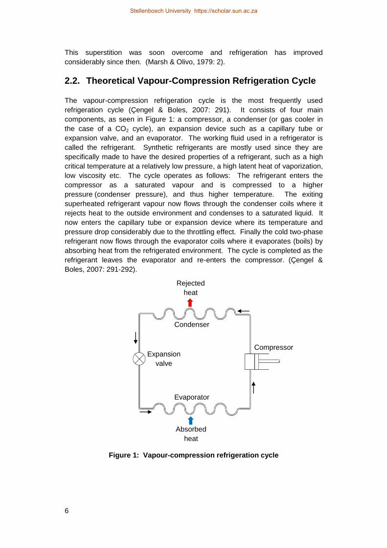
2.2. Theoretical Vapour-Compression Refrigeration Cycle

The vapour-compression refrigeration cycle is the most frequently used

refrigeration cycle (Çengel & Boles, 2007: 291). It consists of four main

components, as seen in Figure 1: a compressor, a condenser (or gas cooler in

the case of a CO2 cycle), an expansion device such as a capillary tube or

expansion valve, and an evaporator. The working fluid used in a refrigerator is

called the refrigerant. Synthetic refrigerants are mostly used since they are

specifically made to have the desired properties of a refrigerant, such as a high

critical temperature at a relatively low pressure, a high latent heat of vaporization,

low viscosity etc. The cycle operates as follows: The refrigerant enters the

compressor as a saturated vapour and is compressed to a higher

pressure (condenser pressure), and thus higher temperature. The exiting

superheated refrigerant vapour now flows through the condenser coils where it

rejects heat to the outside environment and condenses to a saturated liquid. It

now enters the capillary tube or expansion device where its temperature and

pressure drop considerably due to the throttling effect. Finally the cold two-phase

refrigerant now flows through the evaporator coils where it evaporates (boils) by

absorbing heat from the refrigerated environment. The cycle is completed as the

refrigerant leaves the evaporator and re-enters the compressor. (Çengel &

Boles, 2007: 291-292).

Figure 1: Vapour-compression refrigeration cycle


7

2.3. Carbon Dioxide (CO2) Transcritical Refrigeration Cycle

Figure 2 shows a basic CO2 transcritical refrigeration cycle. It is similar to the

conventional cycle discussed in section 2.2; the only difference is the

replacement of the condenser with a gas cooler and the use of a different

compressor suited for CO2 refrigerant. It is called a gas cooler since it may, in

certain circumstances, contain only supercritical gas as opposed to two-phase

flow in a condenser. Furthermore, it operates at higher pressures due to CO2’s

relatively higher pressure needed for the same temperature as compared to

synthetic refrigerants, and hence it must be designed for this purpose. More

information on the CO2 transcritical cycle and modifications to the cycle can be

seen in Sarkar (2010).

2.4. Refrigerant Properties

To select a refrigerant to use in a vapour-compression refrigeration cycle it is

necessary to first identify the properties of the different refrigerants and to

consider its application, whether for household refrigeration or large scale

refrigeration. The desired properties of a refrigerant will be discussed, the

Figure 2: CO2 refrigeration cycle

Compressor Internal heat exchanger

Evaporator

Gas cooler

Capillary

tube


8

properties of CO2, and finally a comparison is made between the different

refrigerants.

2.4.1. Ideal Properties of a Refrigerant

A refrigerant is a substance that is able to easily absorb and reject a large

quantity of heat usually through phase change. According to Trott and Welch

(2000: 28) the ideal properties for a refrigerant are: a high latent heat of

vaporization, high density suction gas, non-corrosive, non-flammable and non-

toxic, a working range outside the triple point and critical temperature,

compatibility with lubricating oil and component materials, reasonable working

pressures that are not below atmospheric pressure nor too high, a high dielectric

strength especially for hermetic compressors, low cost, environmentally friendly,

and finally easy leak detection. Other properties include chemical stability at

operating conditions, a high thermal conductivity and low viscosity (ASHRAE-

Fundamentals, 2001: 19.1).

2.4.2. Properties of Carbon Dioxide

Carbon dioxide is a naturally occurring gas that is readily obtainable at low cost,

non-toxic, non-flammable, has a low global warming potential (GWP), zero ozone

depletion potential (ODP), and is compatible with most materials (Nellis & Klein,

2002). This has led to renewed interest in using CO2 as a potential alternative to

synthetic refrigerants. Carbon dioxide has a relatively low critical temperature of

30.98 . This low critical point allows for it to be used easily for carrying out

technical processes within the transcritical or super critical region. In terms of

thermodynamics, carbon dioxide serves as a well-known reference for a

molecule with a strong quadruple moment and as a testing fluid for calibration

purposes. (Span & Wagner, 1996). Carbon dioxide has a very high critical

pressure of 7.3773 MPa, which makes it more challenging to use as a refrigerant,

and also more inefficient in most circumstances due to higher expansion losses,

through throttling expansion devices, than other refrigerants. The triple point

temperature and pressure of carbon dioxide, is relatively easily obtainable. Due

to the relative ease at which the triple point and critical point of CO2 is reached, it

is used frequently for scientific study of the processes that an element undergoes

in these two extremes. Span & Wagner (1996) has done remarkable work at

developing an equation of state for CO2 that can be used from the triple-point

temperature to 1100 K at pressures up to 800 MPa. This equation of state is in

the form of a fundamental equation explicit in the Helmholtz free energy, which is

a function of density and temperature only. It describes all necessary

thermodynamic properties to within their experimental uncertainty, and a

reasonable description even in the immediate vicinity of the critical region. The

equation doesn’t use any complex coupling to a scaled equation of state, thus

making it very easily implementable within computer codes. (Span & Wagner,


9

1996). Therefore the equation of state from Span & Wagner (1996) was used to

determine the properties of CO2 in the refrigeration cycle simulation program

written for this thesis.

2.4.3. Refrigerant Comparison

In order to choose the refrigerant for a particular application it is first necessary to

compare the different refrigerant’s performance per unit of refrigeration effect

achieved. For this, an ideal refrigeration cycle is assumed that operates at the

design temperatures of the study in hand. The use of an ideal cycle simplifies

calculations and gives good initial insight into possible performance, but actual

performance may be somewhat different. In most cases the assumptions are

that the suction gas is saturated (1), the compression is adiabatic or at constant

entropy (1-2), the heat rejection (2-3) and - absorption process (4-1) is isobaric

with no pressure drop, the condenser fluid leaves as a saturated liquid (3), and

the expansion process follows an isenthalpic throttling process (3-4). In this

study the evaporator temperature is set at 258 K and condenser temperature is

at 303 K. Figure 3 shows the ideal CO2 cycle operating at these design

temperatures.

Figure 3: Ideal CO2 refrigeration cycle operating at 258 K and 303 K

Table 1 shows the refrigerant performance per kilowatt of refrigeration for a few

commercial refrigerants used as well as R-12 refrigerant. The data was

calculated assuming the same ideal refrigeration cycle and design temperatures

of 258 K (≈ -15 ) for evaporation and 303 K (≈ 30 ) for condensation as

described before.

-450 -400 -350 -300 -250 -200 -150 -100 -50 00

1000

2000

3000

4000

5000

6000

7000

8000

Enthalpy, h [kJ/k ]

Pre

ssure

, P

[kP

a]

1

2 3

4 -15

30


10

Table 1: Comparative refrigerant performance per kilowatt of refrigeration

Refrigerant

ASHRAE

no.

Evapo-

rator

Pressure,

MPa

Con-

denser

Pressure,

MPa

Com-

pression

Ratio

Net-

Refriger-

ating

Effect,

kJ/kg

Refrig-

erant

Circu-

lated,

g/s

Specific

Volume

of Suction

Gas,

m3/kg

Com-

pressor

Displace-

ment, L/s

Power

Con-

sump-

tion,

kW

Coeffi-

cient of

Perfor-

mance

Comp.

Dis-

charge

Temp.,

K

R-744

(CO2) 2.281 7.189 3.15 133.25 7.50 0.0165 0.124 0.368 2.72 343

R-290 0.291 1.077 3.71 279.88 3.57 0.1542 0.551 0.211 4.74 320

R-410A 0.481 1.88 3.91 167.68 5.96 0.0542 0.318 0.227 4.41 324

R-12 0.183 0.745 4.07 116.58 8.58 0.0914 0.784 0.213 4.69 311

R-600a 0.089 0.407 4.60 262.84 3.80 0.4029 1.533 0.220 4.55 318

R-134a 0.164 0.770 4.69 149.95 6.66 0.1223 0.814 0.217 4.60 309

R-717

(Ammonia) 0.236 1.164 4.94 1102.23 0.91 0.5106 0.463 0.207 4.84 371

(Modified from ASHRAE-Fundamentals (2001: 19.8))

From the table above it is seen that the CO2 cycle has a coefficient of

performance that is somewhat lower than the rest for this operating case.

However it has other advantageous characteristics such as the lowest

compression ratio, the lowest specific volume of suction gas and also the lowest

compressor displacement rate. The lower compressor displacement rate directly

signifies that small compressors may be used. The use of small compressors

simplifies design for such a high pressure operating environment. The COP of

the system may be improved by exploiting the high pressure difference

expansion process by using an alternative work recovering device such as a

vortex tube or piston expander etc. For example, implementing an isentropic

work recovering expansion device for the CO2 cycle and using the recovered

work to reduce compression power consumption it can be shown, ideally, that the

COP may be improved to a value of 4.84 (sample calculations can be seen in

Appendix A1). Table 2 illustrates how the cycle’s performance would change in

comparison to isenthalpic expansion with no work recovery.

Table 2: Work recovering device versus normal throttling device

Refrigerant

ASHRAE no.

Evapo-

rator

Pressure,

MPa

Con-

denser

Pressure,

MPa

Com-

pression

Ratio

Net-

Refriger-

ating

Effect,

kJ/kg

Refrig-

erant

Circu-

lated,

g/s

Specific

Volume

of

Suction

Gas,

m3/kg

Com-

pressor

Displace-

ment, L/s

Power

Con-

sump-

tion,

kW

Coeffi-

cient of

Perfor-

mance

Comp.

Dis-

charge

Temp.,

K

R-744 (CO2)

isenthalpic

expansion

2.281 7.189 3.15 133.25 7.50 0.0165 0.124 0.368 2.72 343

R-744 (CO2)

isentropic

expansion

with work

recovery

2.281 7.189 3.15 151.14 6.62 0.0165 0.109 0.207 4.84 343

The inclusion of a work recovering isentropic expansion device increases the net

refrigerating effect; therefore, decreasing the mass flow rate and compressor

displacement rate. The lower mass flow rate reduces the total compressor power

consumption needed; furthermore the assumption that 100% of the work

recovered is used by the compressor means that the compressor power is


11

drastically reduced. The lowered compressor power consumption translates to a

significantly improved COP. The cycle’s actual COP may be somewhat different;

nonetheless, this serves as a good illustration of the potential for increasing the

cycle’s COP.

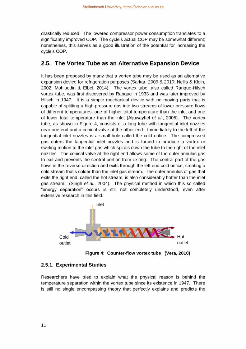
2.5. The Vortex Tube as an Alternative Expansion Device

It has been proposed by many that a vortex tube may be used as an alternative

expansion device for refrigeration purposes (Sarkar, 2009 & 2010; Nellis & Klein,

2002; Mohiuddin & Elbel, 2014). The vortex tube, also called Ranque-Hilsch

vortex tube, was first discovered by Ranque in 1933 and was later improved by

Hilsch in 1947. It is a simple mechanical device with no moving parts that is

capable of splitting a high pressure gas into two streams of lower pressure flows

of different temperatures; one of higher total temperature than the inlet and one

of lower total temperature than the inlet (Aljuwayhel et al., 2005). The vortex

tube, as shown in Figure 4, consists of a long tube with tangential inlet nozzles

near one end and a conical valve at the other end. Immediately to the left of the

tangential inlet nozzles is a small hole called the cold orifice. The compressed

gas enters the tangential inlet nozzles and is forced to produce a vortex or

swirling motion to the inlet gas which spirals down the tube to the right of the inlet

nozzles. The conical valve at the right end allows some of the outer annulus gas

to exit and prevents the central portion from exiting. The central part of the gas

flows in the reverse direction and exits through the left end cold orifice, creating a

cold stream that’s colder than the inlet gas stream. The outer annulus of gas that

exits the right end, called the hot stream, is also considerably hotter than the inlet

gas stream. (Singh et al., 2004). The physical method in which this so called

“energy separation” occurs is still not completely understood, even after

extensive research in this field.

Figure 4: Counter-flow vortex tube

2.5.1. Experimental Studies

Researchers have tried to explain what the physical reason is behind the

temperature separation within the vortex tube since its existence in 1947. There

is still no single encompassing theory that perfectly explains and predicts the

Inlet

Cold

outlet

Hot

outlet

(Vera, 2010)


12

working principle of the vortex tube. Many have experimentally investigated the

influence of the vortex tube’s geometric properties on its performance. Eiamsa-

ard and Promvonge (2007) provides a detailed review of the different

researchers’ results. The researchers did not all record the same or all the

necessary variables, thus making it a nearly impossible task to compare their

results. Geometric properties that were varied by researchers include tube

diameter, inlet nozzle diameter, number of inlet nozzles, cold orifice diameter and

hot outlet area. Other parameters that were also varied include inlet mass flow

rate, inlet pressure, outlet pressure (most experiments were however done with

the outlet being atmospheric pressure) and cold mass fraction (obtained by

varying the hot outlet area).

Christensen et al. (2001) did an experimental study in using the vortex tube as an

alternative expansion device in a CO2 transcritical refrigeration cycle. They found

that the vortex tube produces an enthalpy separation, and therefore in an ideal

gas resulted in a temperature separation. However, for the CO2 in the

refrigeration cycle, which behaves more like a real gas, there is a small

temperature split in certain circumstances and no split in temperature when the

gas becomes two-phase during expansion. Their proof as to why this occurs is

as follows:

Supposing that enthalpy h is a function of temperature T and pressure P, i.e.

h=h(T,P), then the total differential of h is:

(

) (

)

(2.1)

Noting that (

) and using Maxwell’s relations this can be written as:

( (

))

(2.2)

For an ideal gas the last part is equal to zero (by substitution of ideal gas

equation ) . i.e.:

(

)

(2.3)

The remaining relation, , therefore means that a change in enthalpy

directly signifies a change in temperature for an ideal gas. For a real gas this last

part, equation (2.3), is not zero and therefore a change in enthalpy does not

necessarily mean a change in temperature. Thus Christensen et al. (2001)

concluded that the vortex tube would be of little use in a refrigeration cycle if


13

there is no means of separating the two phases and ensuring that the vortex tube

remains in single phase operation.

2.5.2. Analytical and Numerical Studies

From the experiments many researchers have tried to develop a mathematical

formula that would predict the outlet temperatures of the vortex tube, with very

limited success. The formulas developed only worked for certain conditions such

as outlet condition being atmospheric. Also the gas used in most instances is air.

Furthermore, when the vortex tube geometry changed the formula no longer

gave reasonable results, which leads to the belief that the working principle is not

fully explained by the formula in question. Other attempts were to numerically

simulate the vortex tube with CFD programs such as Fluent, StarCD etc. These

programs do produce results that correlate well with the vortex tube’s

performance, however only if the gas which is used exhibits ideal gas behaviour;

since most models used in CFD make use of an ideal gas relation for the state of

the fluid.

2.5.3. Geometrical Properties of the Vortex Tube

Researchers have focused their efforts mainly on finding the optimal geometrical

shape and properties of the vortex tube to give the required output which is either

one of two: maximum temperature difference output or maximum cooling output.

Uses for maximum temperature difference output include spot cooling and

cryogenic cooling applications (Nellis & Klein, 2002) amongst others. Maximum

cooling output is used mainly in refrigeration cycles, which is the topic of this

project.

Through years of experimentation researchers have stipulated what they have

found as the optimal design for a vortex tube. It is worth mentioning that all

researchers haven’t reached the exact same design parameters, some even

contradicting each other’s findings; thus it is very hard to choose which design

advice one should follow. Another important consideration is that this vortex tube

is intended to be used as an expansion device in a CO2 refrigeration cycle in

place of a capillary tube or expansion valve; which means that the vortex tube’s

input and output conditions vary according to the refrigeration cycle’s operation.

The CO2 may be two-phase or close to saturation conditions which means that it

behaves more like a real gas, in which case the vortex tube’s efficiency

improvement potential in the cycle is diminished. The refrigeration cycle’s

varying operating conditions might require a vortex tube with variable geometric

capabilities within operation. A discussion of research results for the geometric

properties of a vortex tube follows beneath. Note that these geometric properties

were determined mostly by using air, which exhibits ideal gas behaviour, as

working fluid.


14

2.5.3.1. Length to Tube Diameter Ratio

The length of tube has a significant influence on the performance of the vortex

tube since it provides room for the swirling flow to develop and ultimately

separate into two streams of flow, one being colder and one hotter than the inlet

flow. Yilmaz et al. (2009) reported from their literature survey that the length of

tube significantly influences its performance, the optimum L/D ratio is a function

of other geometrical and operational parameters, and that L/D beyond 45 has no

further effect or improvement on performance. Saidi and Valipour (2003) have

experimented and found that the optimum range of L/D ratio is between 20 and

55.5. Singh et al. also found that the length of tube has no effect when it’s

increased beyond 45 diameters long (Singh et al., 2004). Eiamsa-ard and

Promvonge (2007) found that L/D should be around 20 for optimum performance.

Others still have suggested that L/D higher than 10 is sufficient.

Behera et al. (2005) stipulated that maximum temperature separation is obtained

by lengthening the tube up to where the stagnation point is furthest from the inlet

nozzle and just within the length of the tube. Thus from all the research it is

evident that depending on what inlet pressures the vortex tube is subjected to the

length needed would be different. Also Promvonge and Eiamsa-ard (2005) show

that an insulated vortex tube gives higher efficiency and temperature separation;

therefore a shorter tube may be used. Considering all above, a length of 20D or

more would be a good design criterion for a vortex tube, it would in most cases

mean that the stagnation point lies within the vortex tube and thus maximum swirl

is used to allow higher energy separation to be achieved.

2.5.3.2. Inlet Nozzle Diameter/Area

The inlet nozzle is a crucial component of the vortex tube. It creates the vortex

flow (swirling flow) within the vortex tube which causes the energy separation. In

order to achieve the best performance of the vortex tube, the Mach number at the

exhaust of the inlet nozzle should be as high as possible, the pressure loss over

the inlet nozzle should be as low as possible, and the momentum flow at the

exhaust should be as large as possible (Yilmaz et al., 2009). The nozzle outlet

diameter should be not too small otherwise it would cause a higher pressure drop

over it, but it should also not be too large, in which case it would fail to produce a

high velocity flow and hence not a strong enough vortex. Both these extremes

would cause a low diffusion of kinetic energy and thus a low temperature

separation. The inlet nozzle should be located as close as possible to the cold

outlet orifice to yield high tangential velocities near the orifice and hence high

temperature separation (Eiamsa-ard & Promvonge, 2007).


15

2.5.3.3. Vortex Tube Diameter

The diameter of the vortex tube is an important parameter in the design since it is

the tube’s inner wall which ultimately causes the swirling motion of the incoming

tangential flow. Past researchers have experimented with vortex tube diameters

as low as 4.4 mm and as high as 800 mm (Eiamsa-ard & Promvonge, 2007).

Larger diameter vortex tubes are generally used for gas liquefication and

separation (Yilmaz et al., 2009).

According to a CFD simulation of a vortex tube done by Aljuwayhel et al. (2005),

reducing the diameter from 2 cm to 1.5 cm led to an increase in cold temperature

drop by 1.2 K, and increasing the diameter from 2 cm to 3 cm decreases the cold

temperature drop by 6.5 K. These simulations were run with the same inlet

pressure and conditions, thus it is evident that the larger the diameter of the tube,

the lower the angular velocity of the flow is, and thus the less energy separation

occurs. Depending on the inlet pressure, the smaller the diameter of the vortex

tube is the higher the energy separation is up to a certain diameter. If the

diameter is made too small it would produce considerably higher back pressure

due to the high density of gas in the tube, and therefore, the tangential velocities

between the periphery and the core would not differ much while high axial

velocities are encountered in the core region as the gas tries to escape. The low

tangential velocities cause low diffusion of kinetic energy which also means low

temperature separation. With that said, a very large tube diameter would also

result in lower overall tangential velocities both in the periphery and in the core,

and hence lower temperature separation. (Aljuwayhel et al., 2005).

Researchers have focused their attention more on the L/D ratio rather than the

diameter of the tube. The diameter of the tube depends on the inlet pressure. It

is seen that tangential velocity (or swirl) causes the energy separation. The

vortex tube diameter should be chosen within the two extremes mentioned in the

previous paragraph. However, it is seen that designs lean towards smaller tubes

for better temperature separation.

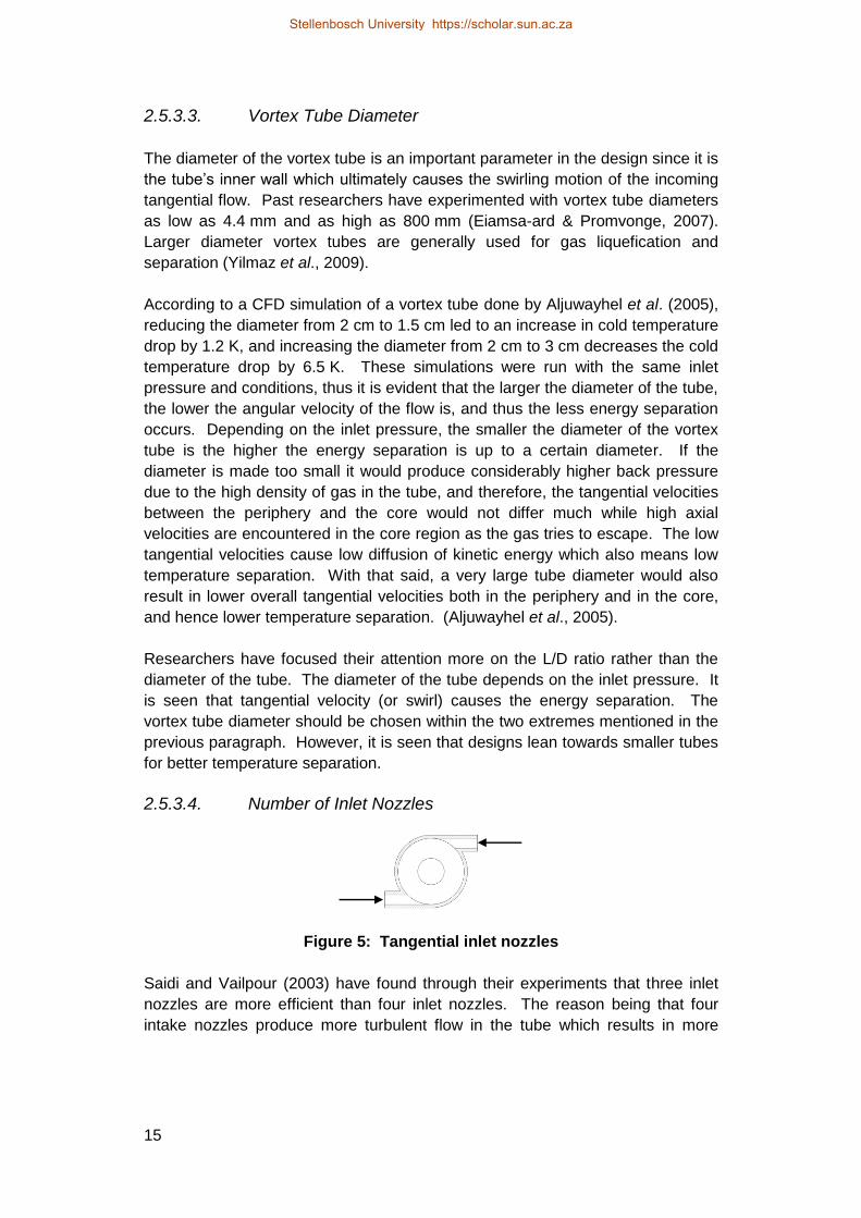
2.5.3.4. Number of Inlet Nozzles

Figure 5: Tangential inlet nozzles

Saidi and Vailpour (2003) have found through their experiments that three inlet

nozzles are more efficient than four inlet nozzles. The reason being that four

intake nozzles produce more turbulent flow in the tube which results in more


16

mixing between the cold and hot layers of flow, and thus less energy separation,

hence lower cold temperature difference and lower efficiency. Promvonge and

Eiamsa-ard (2005) have experimented with 1, 2 and 4 inlet nozzles and found

that 4 nozzles gave better temperature separation and efficiency. Their

conclusion reached was that increasing the number of nozzles helped to speed

up the flow, to increase the mass flow rate and to generate stronger swirl flow in

the vortex tube.

Hamdan et al. (2013) states that there is an optimum number of nozzles for a

vortex tube of specific geometry and operating conditions and found that 4 inlet

nozzles produced the best energy separation. Furthermore, they found that the

inlet nozzles should be tangential to the vortex tube periphery.

2.5.3.5. Cold Orifice Diameter

The cold orifice diameter is one of the most important parameters in the design of

a vortex tube, since this component is integral to the temperature separation

effect of the vortex tube. If the orifice is too large relative to the tube’s diameter,

inlet gas from the inlet nozzles would escape directly into the cold outlet stream

instead of creating the necessary vortex flow in the vortex tube. This would result

in poor temperature separation due to lack of vortex flow near the cold orifice and

also due to mixing of the inlet gas and the cold outlet stream. However, if the

cold orifice is too small there is a high pressure drop over the cold orifice,

therefore a high back pressure inside the vortex tube and hence a smaller

pressure drop across the inlet nozzles. This would cause insufficient vortex flow

in the tube and thus lower temperature separation. (Yilmaz et al., 2009).

Saidi and Valipour (2003), as well as Promvonge and Eiamsa-ard (2007) found

that the optimum cold orifice diameter to vortex tube diameter should be 0.5. A

review done by Yilmaz et al. (2009) suggests that the optimum cold orifice

diameter should be between 0.4D and 0.6D.

2.5.3.6. Hot Outlet Area or Cold Mass Fraction

The hot outlet area is described as the area between the hot valve (conical

control valve, shown on the right in Figure 4) and vortex tube wall. The hot outlet

area is normally variable by adjusting the hot valve’s axial position. The hot

outlet area is closely related to the cold mass fraction. A change in position of

the control valve alters the hot outlet area and hence causes a difference in back

pressure by the hot valve and thus changes the fraction of gas allowed to escape

through the hot end; therefore the cold fraction changes too.

It is claimed by many research experimental articles that the cold mass fraction is

the only factor that needs to be controlled in order for the vortex tube to achieve


17

maximum temperature separation or maximum cooling efficiency. Gupta et al.

(2012) state that a cold mass fraction of 0.4 gives the maximum temperature

drop and maximum cooling effect is seen between 0.35 and 0.65. The cooling

effect is a function of the temperature drop and the mass flow rate of cold gas.

Nimbalkar and Muller (2009) claims that a cold fraction of 0.6 gives the maximum

energy separation or cooling effect.

2.5.4. Thermo-Physical Parameters

The performance of the vortex tube is affected by the thermo-physical properties

of the gas used, such as inlet flow temperature and pressure, moisture content

and specific heat ratio etc. (Saidi & Valipour, 2003). Increasing the inlet pressure

increases the temperature separation up to a certain point. As the pressure is

increased the flow inlet velocity increases up to the point where it becomes

choked. A further increase in pressure only causes a slowly increasing

temperature difference. The efficiency also increases up to the point that the flow

becomes choked and then decreases as the energy separation decreases.

Efficiency and cold temperature difference decreases with increasing moisture

content of the inlet gas. Gases with higher specific heat capacity ratio attain

higher temperature difference. (Saidi & Valipour, 2003).

2.6. The Finite Volume Method

The finite volume method provides for a definitive method of expressing the

conservation equations of fluid flow in a discretised form that can easily be

implemented within a computer code. The flow field is divided into a finite

number of control volumes (CV), hence the name finite volume method. The

intention of this project is to model fluid flow in small diameter refrigerator tubes,

therefore a one-dimensional (1-D) model would suffice. A simple derivation of

the necessary discretised equations is to follow; for a more detailed discussion

refer to Patankar (1980), and Versteeg and Malalasekera (2007). The three

equations of change that governs 1-D fluid flow and heat transfer of a

compressible fluid are (as derived from Versteeg and Malalasekera (2007:24)):

conservation of mass:

( )

(2.4a)

conservation of momentum:

( )

( )

(2.4b)

and conservation of energy:


18

( )

( )

( )

(2.4c)

where is the density, is time, is axial direction, is radial direction, is the

velocity, is the pressure, is the shear stress on the fluid due to friction on

the tube walls, is the specific internal energy, is the average friction shear

stress, and finally the source term is used to incorporate external radial heat

transfer.

It can be seen that the three conservation equations all have a similar form and

can therefore be written for a general variable, , as:

( )

( )

(2.5)

where , and for the three conservation equations respectively.

This equation is referred to as the transport equation for property .

Figure 6 shows the control volume used in the control volume method for the

transportation of the general variable . The finite volume method involves the

integration of the conservation equations over a control volume. This leads to:

∫ ( )

∫

( )

∫

(2.6)

Using Gauss’s divergence theorem the second integral can be represented by a

surface integral as:

∫

( )

∫( )

(2.7)

This states that the volume integral is equal to the surface integral over the entire

bounding surface of the control volume. The direction of is normal to the

surface which bounds the control volume integrated, this is the application of

Gauss’s divergence theorem. In this case only flow in the z direction is

𝜃

𝑧

𝜌𝜙𝑣𝑧

𝑟

Figure 6: Control volume for tube fluid flow


19

encountered therefore the area over which this integral is calculated would be the

inlet and outlet control volume cross-sectional areas.

Since a transient time-dependent simulation model is developed, it is first

necessary to decide which temporal discretisation scheme to use. There are

three well known schemes that exist, namely: fully explicit, Crank-Nicolson, and

fully implicit. The fully explicit scheme uses only old time step values to calculate

the new time step value. This allows for easy computation; however there is a

stringent limitation to time step size due to the Scarborough criterion which states

that all coefficients of the discretised equation must be of the same sign, normally

all positive, to ensure bounded and physically realistic results (Versteeg &

Malalasekera, 2007: 247). The fully explicit scheme also possesses no intrinsic

means for correcting or ensuring that the conservation equations remain

conserved as time progresses. In the fully implicit scheme the old time value is

treated as a source term and new time values are used to calculate the new

values. This scheme is therefore iterative in nature; also it is unconditionally

stable for any time step size since all discretisation equation coefficients are

positive. However since the accuracy of the scheme is first-order in time, small

time steps are needed to ensure the accuracy of the results (Versteeg &

Malalasekera, 2007: 249). The Crank-Nicolson scheme uses a weighting of half

the new - and half the old time step values to compute the new values. This

method is more robust than the fully explicit method, in that it has a less

restrictive time step size limit. Other schemes with a different weighting between

new – and old time step values also exist but are of no interest to this study.

The robustness and unconditional stability of the fully implicit scheme are the

reasons for it being the method of choice for transient simulation purposes.

Furthermore the iterative nature of this scheme ensures that the conservation

equations remain conserved as time progresses. Therefore, all subsequent

derivations will focus on the implementation of the fully implicit scheme.

Integration of a conservation equation over a control volume, as shown in Figure

7, yields a discretised equation at the node, P, of the control volume (usually at

its center). The discretised equation contains neighbouring node values

depending on the discretisation scheme used to represent face values of the

current control volume. To illustrate how a differential conservation equation is

transformed into a usable discretised equation, the discretised form of the

Figure 7: Notation used in the control volume discretisation

P E W

w e

( 𝑧)𝑒− ( 𝑧)𝑤+

( 𝑧)𝑒 ( 𝑧)𝑤

( 𝑧)𝑤− ( 𝑧)𝑒+


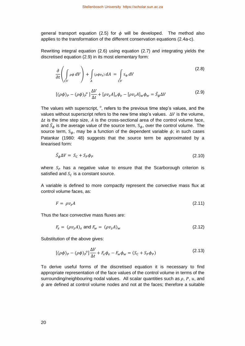
20

general transport equation (2.5) for will be developed. The method also

applies to the transformation of the different conservation equations (2.4a-c).

Rewriting integral equation (2.6) using equation (2.7) and integrating yields the

discretised equation (2.9) in its most elementary form:

( ∫

) ∫( )

∫

(2.8)

[( ) ( ) ]

[ ] [ ]

(2.9)

The values with superscript, o, refers to the previous time step’s values, and the

values without superscript refers to the new time step’s values. is the volume,

is the time step size, is the cross-sectional area of the control volume face,

and is the average value of the source term, , over the control volume. The

source term, , may be a function of the dependent variable ; in such cases

Patankar (1980: 48) suggests that the source term be approximated by a

linearised form:

(2.10)

where has a negative value to ensure that the Scarborough criterion is

satisfied and is a constant source.

A variable is defined to more compactly represent the convective mass flux at

control volume faces, as:

(2.11)

Thus the face convective mass fluxes are:

( ) and ( ) (2.12)

Substitution of the above gives:

[( ) ( ) ]

( )

(2.13)

To derive useful forms of the discretised equation it is necessary to find

appropriate representation of the face values of the control volume in terms of the

surrounding/neighbouring nodal values. All scalar quantities such as , , , and

are defined at control volume nodes and not at the faces; therefore a suitable


21

interpolation or other consistent discretisation scheme has to be used to

represent face values in terms of the nodal values.

For example for face values of linear interpolation (also called central

differencing), with reference to Figure 7, yields the following:

+(1- ) and +(1- ) (2.14)

where ( ) ( )

and ( ) ( )

According to Patankar (1980: 34) it is not necessary to use the same

discretisation scheme for every variable; the discretisation scheme chosen for a

variable depends on how well it describes the physical behaviour of that variable.

Versteeg and Malalasekera (2007: 141) state that the most fundamental

properties that a discretisation method requires are conservativeness,

boundedness and transportiveness. Conservativeness entails using a consistent

expression for the flux of a property through a common face in adjacent control

volumes. This means that leaving one control volume through a face must

enter the adjacent control volume through the same face, thus ensuring

conservation of through the whole simulation domain. Boundedness ensures

that the results are physically realistic in the sense that the values of internal

nodes are bounded by its boundary values in the absence of internal sources.

For the boundedness requirement all coefficients of the nodal values in the

discretised equation must satisfy the Scarborough condition in that they are all of

the same sign (usually all positive). This ensures that an increase in at one

node would result in an increase in in the neighbouring nodes.

Transportiveness in a discretisation scheme ensures that the flow direction is

taken into account by ensuring that the value of node P is predominantly

influenced by the upstream neighbouring node, as is physically occurring, and

not the downstream neighbour.

The central differencing scheme requires small control volumes, hence a large

number of control volumes, and does not recognize the direction of flow, i.e. does

not possess the transportiveness property. The simulation model developed will

make use of the minimum amount of control volumes possible, to keep

computation time to a minimum, therefore it was decided to use the upwind

differencing scheme. This scheme is relatively robust in the sense that it can

produce physically realistic results with the minimum amount of control volumes

and it possesses all three fundamental properties of a discretisation scheme.

A development of the discretised equation of the general variable using the

upwind differencing scheme is to follow.

If the flow is in the positive direction ( ) > 0, ( ) > 0 ( > 0, > 0):


22

and (2.15)

Substitution of the upwind differencing values into the discretised equation yields:

[( ) ( ) ]

( )

(2.16)

Rearranging gives:

[

] [

]

(2.17)

If the flow is in the negative direction ( ) < 0, ( ) < 0 ( < 0, < 0):

and (2.18)

Substitution of the upwind differencing values into the discretised equation yields:

[( ) ( ) ]

( )

(2.19)

Rearranging gives:

[

] [

]

(2.20)

Identifying the coefficients of , , and as , , and respectively,

equations (2.17) and (2.20) can be written in general form as:

(2.21)

where:

( ) ( )

( ) ( )

Discretised equations of the form (2.21) must be set up at each node in the

simulation domain. The discretised equation is modified for boundary control

volumes to incorporate boundary conditions.

The equations are now written in the form:


23

(2.22)

where is the variable being solved.

The set of equations for the simulation nodes are all written in a matrix starting

with the first node’s equation in the first row and continuing till the last node’s

equation in the last row. The resulting matrix has a tri-diagonal form and can

then be solved by forward elimination and back-substitution. This algorithm,

called the tri-diagonal matrix algorithm (TDMA), can be implemented in a for-loop

and is less computationally expensive than direct methods. It requires a number

of computations in the order of versus for direct methods, where is

the number of variables being solved. A detailed description of the TDMA

algorithm can be obtained in Versteeg and Malalasekera (2007: 213).

3. DETERMINING THE THERMODYNAMIC STATE

Simulation of a CO2 refrigeration cycle would necessitate an equation of state

that is not only accurate, but also computationally inexpensive. The accurate

equation of state from Span and Wagner (1996) involves no complex coupling to

a scaled equation and thus makes it less computationally expensive and easier

to program.

3.1. CO2 Equation of State from Span and Wagner

The equation of state from Span and Wagner (1996) is used in the simulation

program of the refrigeration cycle to determine the thermodynamic properties of

CO2. This equation is in the form of a fundamental equation explicit in the

Helmholtz energy, A, which is a function of density and temperature T. The

equation is structured to use the dimensionless Helmholtz energy ( )

which is split into a part depending on the ideal-gas behaviour and a part to

take into account the residual fluid behaviour , namely:

( ) ( ) ( ) (3.1)

where is the inverse reduced temperature and is the reduced

density. Both the temperature T and the density are reduced with their critical

values, K and kg/m3, respectively.

All thermodynamic properties of a pure substance can be obtained by combining

derivatives of eq. (3.1), because the Helmholtz energy as a function of density

and temperature is one form of a fundamental equation. Table 3 in Span and

Wagner (1996: 1517) gives the thermodynamic property relations to the reduced

Helmholtz energy and its derivatives. In the context of having a detailed


24

discussion of how the equation of state is solved with other variables such as

density and specific internal energy, it was decided to have the thermodynamic

property relations as a reference in the table below.

Table 3: Relations of the thermodynamic properties to the dimensionless

Helmholtz function

Property and common

thermodynamic definition

Relation to the dimensionless Helmholtz energy

and its derivativesa

Pressure:

( ) ( )

( )

Entropy:

( ) ( )

( )

(

)

Internal energy:

( ) ( )

( )

(

)

Enthalpy:

( ) ( ) ( )

( )

(

)

Isochoric heat capacity:

( ) ( )

( )

(

)

Isobaric heat capacity:

( ) ( )

( )

(

)

(

)

Speed of sound:

( ) √( )

( )

(

)

(

)

a *

+ , *

+ , *

+ , *

+ , and *

+.

Relations and the coefficients used for the ideal-gas part of the dimensionless

Helmholtz function and its derivatives can be obtained from Table 28 and 27,

respectively, of Span and Wagner (1996: 1540-1541). Relations and the

coefficients used for the residual part of the dimensionless Helmholtz function

and its derivatives can be obtained in Table 32 and 31, respectively, of Span and

Wagner (1996: 1544-1545).


25

The MATLAB script file, CO2_Property.m, written to calculate the thermodynamic

properties, as shown in Table 3, from a given density and temperature using

Span and Wagner’s equation can be seen in Appendix B1. All coefficients of

Span and Wagner’s equation are stored in .mat format and called when needed.

3.2. Saturated Property Determination

The vapour pressure and densities of saturated vapour and saturated liquid

can be determined by solving the following equations simultaneously. These

equations correspond to the equality of temperature, pressure and specific Gibbs

energy (Maxwell criterion) in the coexisting phases (Span and Wagner, 1996:

1516).

( )

(3.2a)

( )

(3.2b)

(

) (

) ( )

( ) (3.2c)

Span and Wagner (1996: 1524-1525) give simple correlations, based on

temperature, for the vapour pressure, saturated vapour density and saturated

liquid density, which can be used as a very good initial guess in a program to

solve the above equation set. The correlations are:

( )

[∑ (

)

] (3.3)

for the vapour pressure, where , ,

, , , , and .

(

) ∑ (

)

(3.4)

for the saturated liquid density, where , ,

, , ,

,

and

.

and finally


26

(

) ∑ (

)

(3.5)

for the saturated vapour density, where , ,

, , ,

, ,

and

.

Since the thermodynamic properties of CO2 are functions, as shown in Table 3,

its derivatives will in themselves be functions as well. Therefore the Newton-

Raphson method (Chapra, 2008: 144) can be applied to simultaneously solve

equations such as equation set (3.2). Once these equations are solved for a

specific temperature, the calculated saturated density and temperature can be

used to calculate all other saturated properties using the function script file

CO2_Property.m. The MATLAB script, CO2_Sat_Prop_at_T.m in Appendix B2,

calculates saturated properties using equations (3.3-3.5) as initial guesses for , , and and then equations (3.2a-c) are solved using the Newton-Raphson

method. Solving equations (3.2a-c) simultaneously for temperatures from the

triple point up to the critical point in a loop a vector of points can be generated for

any saturated properties, which can then be used to draw saturated property

graphs. The MATLAB script file, CO2_Sat_Prop_at_T_Iteration.m (can be seen

in the project file), is used to create these vectors and plot the graphs.

3.3. Determining Single Phase and Two-Phase Properties

Simulating fluid flow using the control volume approach, one would split up the

flow domain in control volumes of finite size and then simultaneously solve the

three conservation equations namely mass, momentum and energy. The

nonlinear nature of the momentum equation makes it very difficult to solve these

three equations simultaneously using direct methods and therefore an iterative

method such as commonly used in CFD would be adapted. Solving these three

equations simultaneously the density and specific internal energy u of each

control volume are obtained and then the equation of state is used to determine

the pressure, temperature and all other properties; thus linking the mass and

energy equation to the momentum equation.

Since the equation of Span and Wagner uses and T, but only and u are

known; it would be necessary to guess a temperature and use an appropriate

iteration method to find the correct temperature, and consequently all other

properties that satisfy and u. The following two sections explain how the

properties are obtained for the single phase and the two-phase regions. The

third section discusses the logical process of determining whether the fluid is

single - or two-phase, and then selecting the appropriate functions to calculate

the thermodynamic properties, as well as the viscosity and thermal conductivity.


27

3.3.1. Determining Single Phase Properties

The single phase program is easier to implement and understand, thus its

derivation will be explained first. Since one of the variables in Span and

Wagner’s equation is already given, namely the density, it is only required to find

the correct temperature that satisfies the given specific internal energy i.e. u may

be treated as a function of T only at this fixed density. Therefore it is required

that the specific internal energy u( ,T) calculated from the guessed temperature,

or iteratively improved temperature, be equal to the given specific internal energy

. Writing the difference between these two in function form gives:

( ) ( ) (3.6)

This has now reduced to a root finding problem which the Newton-Raphson

method (Chapra, 2008: 144) is well suited for, especially if a good initial guess for

T is available. The error is defined as the absolute value of f.

The new value of T is defined by the Newton-Raphson formula as:

+ ( )

( )

(3.7)

where

( )

( ( ))

( ( )) ( )

(3.8)

Note that is the given specific internal energy and therefore is treated as a

constant in the derivation. The value for ( ) and ( ) are determined

from the equations in Table 3 in a script file called u_and_cv_script.m. This script

file is a shortened version of CO2_Property.m, written only for determining u and

. This shortened version allows time saving in the iteration process as opposed

to using the whole CO2_Property.m script.

The updated temperature is again used to determine new properties and the

whole procedure is repeated until the error reaches a prescribed level. Finally

when the error level is reached all thermodynamic properties are updated using

CO2_Property.m. The script file, CO2_1Ph_Prop_at_rho_and_u.m, written to

determine the single phase thermodynamic properties can be viewed in

Appendix B3.


28

3.3.2. Determining Two-Phase Properties

Assuming a homogeneous mixture for the two-phase fluid a set of four unknowns

emerge. Determining the state from a given density, , and specific internal

energy, , the four unknowns are temperature T, saturated vapour density ,

saturated liquid density , and volume fraction . The temperature and volume

fraction at the old time level or previous iteration can be taken as a good initial

guess. Equations (3.4-3.5) are used to obtain good guesses for and based

on the guessed temperature. Four equations are needed to determine the four

unknowns. These equations are given below.

The two-phase internal energy per volume is represented by:

( ) (3.9a)

The two-phase flow homogeneous density is represented by:

( ) (3.9b)

The vapour and liquid are in equilibrium thus the pressure is equal for both:

( ) ( ) (3.9c)

Also equilibrium between vapour and liquid means that the specific Gibbs energy

g is the same for both phases:

( ) ( ) (3.9d)

The specific Gibbs energy is defined as:

(3.10)

where is the specific enthalpy, T is the temperature, and is the specific

entropy.

Simultaneously solving the four equations (3.9a-d) necessitates an efficient

method and hence the Newton-Raphson method is again implemented (Chapra,

2008: 272-276). First the four equations are written in difference form i.e.

reduced to a root finding problem.

( ) ( ) (3.11a)

( ) ( ) (3.11b)


29

( ) ( ) ( ) (3. 11c)

( ) ( ) ( ) (3. 11d)

Derivatives of these four functions are now developed. Note that and are

the given density and specific internal energy; therefore they are treated as

constants in deriving derivatives of the above functions. Appendix B4 contains

the other derivatives used in the following derivations.

( )

( ) ( ) ( )

(3.12a)

*( )

( ) +

(3.12b)

( ) ( )

*( )

( ) +

(3.12c)

(3.12d)

(3.13)

( )

(

(

)

) (

(

)

)

(3.14a)

( )

( )

*(

)

( )

+

(3.14b)

( )

( )

*(

)

( )

+

(3.14c)


30

(3.14d)

( )

* ( ( )

( )

) +

* ( ( )

( )

) +

(3.15a)

( )

( ( )

( ) (

)

) (3.15b)

( )

( ( )

( ) (

)

) (3.15c)

( )

(3.15d)

The Newton-Raphson method is now applied to simultaneously solve the set of

equations (3.15a-d). To use the Newton-Raphson method for a set of equations

it is necessary to write the equations in matrix form. The formula remains the

same as for solving a single equation in one variable; the only difference is that

the derivative is now replaced by a matrix of derivatives.

The vector of unknowns and the vector of function values (calculated from

equations (3.15a-d)) are:

[

] [

]

The matrix of derivatives is:

[

]


31

The Newton-Raphson formula for updating the vector is:

+ − (3.16)

where − is the inverse of .

All derivatives and function values needed in the Newton-Raphson formula are

obtained by use of the property calculating script CO2_Property.m.

The error is defined as the maximum absolute value of f. The updated

temperature and densities are used again to determine new properties and the

whole procedure is repeated until the error reaches a prescribed level. Finally

when the error level is reached the vapour fraction is calculated and all

homogeneous thermodynamic properties are calculated. The void fraction

obtained is later used to calculate the homogeneous viscosity and thermal

conductivity. The script file written to determine the two-phase thermodynamic

properties, CO2_2Ph_Prop_at_rho_and_u.m, can be viewed in Appendix B5.

3.3.3. Deciding whether the Fluid is Single Phase or Two-Phase

To determine the state of each control volume based on and u it is first

necessary to determine whether it is two-phase or single phase. The fluid phase

is determined with the help of a phase diagram as shown in Figure 8. If a point

( ,u) lies within the polygon it is two-phase else it is single phase. The vectors

used to plot the graph in Figure 8 are saturated density and saturated specific

internal energy. These vectors were generated by the script file,

CO2_Sat_Prop_at_T_Iteration.m as explained in section 3.2.

Figure 8: Phase diagram for CO2

-400 -350 -300 -250 -200 -150 -100

102

103

104

Internal energy, u [kJ/k ]

Density, 𝜌

[k / ]

Two-phase

Single phase

Critical point


32

Figure 9 shows the program logic to decide whether the fluid is single phase or

two-phase. Once determined if the fluid is single - or two-phase the appropriate

script file is called to calculate the thermodynamic properties. The single phase

thermodynamic properties are calculated with CO2_1Ph_Prop_at_rho_and_u.m

as explained in section 3.3.1., and the two-phase thermodynamic properties are

calculated with CO2_2Ph_Prop_at_rho_and_u.m as explained in section 3.3.2.

The thermal conductivity is calculated by the script file CO2_Conductivity.m,

shown in Appendix B6, which uses the equation developed by Scalabrin, Marchi,

Finezzo and Span (2006). The dynamic viscosity is calculated by the script file

Viscosity_CO2.m, shown in Appendix B7, which uses the equation developed by

Fenghour, Wakeham and Vesovic (1998). Both the conductivity and dynamic

viscosity equations are a function of density and temperature. The two-phase

thermal conductivity and dynamic viscosity are calculated based on the

homogeneous flow model with the use of the volume fraction. The MATLAB

script file, CO2_Prop_at_rho_and_u.m, written to calculate all properties

following the logic set out in Figure 9 can be viewed in Appendix B8.

rho>rho_f @ triple point

or

rho<rho_g @ triple point

rho>=rho @ critical

point

u<u_f @ rhou<u_g @ rho

Two-phase

properties

calculated

Single phase

properties

calculated

TrueFalse

False

False

True

TrueTrue False

Figure 9: Program logic to determine the properties of CO2 at a given

density and specific internal energy


33

4. TRANSIENT SIMULATION PROGRAM OF THE CO2 REFRIGERATION CYCLE

A transient simulation program for the basic CO2 refrigeration cycle, containing a

capillary tube as expansion device, is written and will be explained in this

chapter. The one-dimensional finite volume method, as explained in section 2.6,

is used to write the simulation program. The simulation program code may be

viewed in Appendix C. The main program can be viewed in Appendix C1.

4.1. General Model Assumptions

The simulation model is developed under the following assumptions:

The refrigerant is pure CO2 with no oil entrained.

A homogeneous model is used for two-phase flow. This simple model is

easily implemented within a finite volume formulation, and gives results

that are reasonably accurate. It is assumed well suited for the simulation

since the flow is confined to small tubes, thus separated flow is not readily

expected.

No gravity effects are incorporated in the simulation equations since its

effects are assumed negligible for such a small household refrigeration

system. Also the homogenous flow model used ignores gravity effects.

The compressor operates in a continuous manner with no pauses

between suction and expulsion i.e. it sucks and expels gas at the same

instant in time. This allows simplification in programming the simulation

model.

The refrigeration system starts from resting conditions, where the gas in

the system is at equilibrium with the surrounding environmental

temperature and there is no flow.

4.2. Initialising the Simulation Domain

The simulation domain is initialised/created by first defining its geometric

properties (section 4.2.1) and then defining initial conditions for the fluid in the

simulation domain (section 4.2.2). The program code to initialise the simulation

domain can be viewed in Appendix C2.

4.2.1. Defining Geometric Properties of the Simulation Domain

The refrigerator layout being simulated is shown in Figure 10. The whole

refrigerant circuit, from compressor outlet back to compressor inlet forms part of

the simulation domain. External counter-flow water-cooled heat exchangers are

incorporated within the simulation to calculate the heat transferred during


34

operation. The compressor’s effect on the simulation domain is incorporated

through boundary conditions applied to the simulation domain as will be

explained in section 4.3.

The simulation domain is split into a number of control volumes of differing

lengths; closer to inlets and changes in tube diameters the control volumes are

made shorter to enable the simulation to capture the fine changes occurring in

these regions. Stretching of the control volume lengths allows saving on

computing power necessary for the simulation. A stretch ratio is applied to define

the control volume lengths as:

+ (4.1)

where + is the next control volume length, and r is the stretch ratio. A stretch

ratio close to one is however used in order to have a good aspect ratio between

control volume lengths.

Gas cooler

Evaporator

Capillary

tube

Ntot

Ntot -1

1 2 Nev

Ngc 1 2

Compressor 1

2

3

Internal heat exchanger

Figure 10: Basic refrigeration cycle for simulation


35

Control volume numbering of the CO2 refrigerant (simulation domain) starts with

at the compressor outlet and ends with at the compressor inlet.

The gas cooler and evaporator outer tubes contain water which is flowing in the

opposite direction of the CO2 refrigerant in the inner tube. The numbering of the

outer tubes’ control volumes are as indicated in the figure above. It was chosen

to be numbered in this particular order to facilitate programming of the heat

exchange between the water and CO2 control volumes. The number of control

volumes used for the gas cooler, internal heat exchanger, capillary tube and

evaporator are 400, 120, 230 and 300 respectively. For other details such as the

number of control volumes for connecting tubes and transition pieces (for

connection fittings between tubes) refer to the initialise script file in Appendix C2.

4.2.2. Initial Conditions for the Simulation Domain

To start the simulation the initial conditions for each control volume are assigned.

The initial temperature of the water in the outer tubes of the gas cooler and

evaporator is at ambient temperature of 25 . The initial conditions for the CO2

refrigerant were calculated assuming the system is in equilibrium with its outside

environment. The temperature of the CO2 in the system is thus at environmental

temperature:

K (4.2)

The mass of CO2 charged in the system is:

k (4.3)

The volume of the system is calculated by measuring the length and using the

specified inner diameters of the tubes. The properties of the CO2 can now be

calculated based on and T. The properties are calculated by

a script file called CO2_Prop_at_rho_and_T.m, which can be viewed in the

project file. This function can calculate single phase and two-phase properties. It

is determined that the system fluid is two-phase at the initial conditions. To

provide starting conditions for the simulation model it was decided to have all the

saturated fluid in the last control volumes of the high pressure side and saturated

vapour in the rest of the control volumes, including the low pressure side. This is

a fair assumption noting that: i) the highest mass of CO2 and hence fluid would

end up in the high pressure side during and after operation, ii) the refrigerator

design is such that there is a large enough length/volume of tube on the high

pressure side which is lower to the ground than the other tubes, thus enabling

gravity to keep the liquid in the high pressure side. The tubing is laid out in this

manner to avoid liquid from entering the compressor inlet. iii) Furthermore, the

temperature of the low pressure side (with less fluid in it) will go back to the

higher environmental temperature when operation stops; thus the fluid inside


36

would end up being saturated vapour at the environmental temperature once

equilibrium is reached.

4.3. Boundary Conditions for the Simulation Domain

The inlet water temperature for the outer tubes of the external heat exchangers

(gas cooler and evaporator) is 25 . The inlet and outlet boundaries of the

simulation domain of the CO2 refrigerant circuit are dependent on the

compressor’s operating characteristics. Data of the compressor efficiency and

speed was not available; hence, some reasonable assumptions are made in this

section to develop the simulation model. The boundary conditions are continually

updated at the start of each iteration (as needed by the fully implicit temporal

scheme used). A continuous compressing model is adopted for the compressor,

in which the compressor sucks and expels gas at the same instant in time.

The outlet of the simulation domain is the inlet to the compressor. Therefore:

( ) (4.4a)

( ) (4.4b)

( ) (4.4c)

The mass flow rate through the compressor is determined by:

(4.5)

where − is the given compressor displacement volume,

is the assumed speed of the compressor in rpm, and is the

compressor volumetric efficiency. For the compressor used a value of

is calculated to ensure that equation (4.5) satisfies the compressor rated mass

flow rate as determined in section 5.3. Also for the simulation model it is

assumed that the compressor reaches full speed instantly, at t = 0 s.

Since a transient model for the compressor efficiency is not available, it is

decided to use a constant efficiency as determined from a steady-state test point.

There were however no power usage rated by the compressor manufacturer

data; therefore, the compressor efficiency could not be calculated. An isentropic

efficiency of is thus assumed and validated later during

experimentation.

The outlet of the compressor is taken to be at the pressure of the first control

volume in the simulation domain i.e.:


37

( ) (4.6)

To determine the state of the CO2 expelled by the compressor, it is first

necessary to calculate the state following an isentropic process. Then an

isentropic efficiency is applied to determine the actual state. The state is

calculated as follows: For isentropic compression the enthalpy at exit,

, can be determined by the two independent variables at exit already

known i.e. from and . The exit state would be single

phase, thus the script file CO2_1Ph_Prop_at_P_and_s.m (included in the project

file) is used to determine properties from a given pressure and specific entropy.

The actual enthalpy at the outlet of the compressor can be calculated as:

(4.7)

All properties at the outlet of the compressor can now be calculated from the

pressure and enthalpy, i.e. and , with the script file

CO2_1Ph_Prop_at_P_and_h.m (included in the project file).

The compressor discharge specific internal energy is treated as a source term in

the boundary control volume of the energy equation (which is written in the form

of specific internal energy) as shown in section 4.7.2. i.e.:

(4.8)

where is a source of internal energy.

The compressor discharge density is used to calculate the velocity which is

treated as an inlet boundary velocity in the momentum equation as shown in

section 4.7.3. i.e.:

( )

(4.9)

where is the inlet area of the first control volume.

The outlet boundary velocity of the simulation domain is also defined by the

compressor mass flow rate as:

( )

(4.10)

where is the outlet area of the last control volume.


39

To develop relations for the thermal resistances in Figure 11, it is necessary to

first state some common variable definitions, such as Prandtl number and

Reynolds number.

The Prandtl number of the fluid is defined as:

(4.12)

where is the dynamic viscosity, is the isobaric specific heat and is the

thermal conductivity.

The Reynolds number for the flow is:

( )

(4.13)

where is the density, ( ) is the absolute value of the average velocity over

the section considered and is the hydraulic diameter of the flow.

The thermal resistance for the inner tube fluid is defined by:

(4.14)

where is the inner diameter of the inner tube, the length of tube being

considered, and the heat transfer coefficient is

(4.15)

The Nusselt number is

(4.16)

The exponent is 0.3 when the fluid is expected to be cooled and is 0.4 when it's

expected to be heated. is the hydraulic diameter of the flow.

The inner copper tube thermal resistance is defined as:

(

)

(4.17)


40

where and is the inner tube outer and inner diameters, respectively.

is the thermal conductivity of copper, and is the length of tube being

considered.

The thermal resistance for the annulus fluid on the outer side of the inner tube is

defined as:

(4.18)

where is the outer diameter of the inner tube, is the length of tube being

considered and the heat transfer coefficient is

(4.19)

and

(4.20)

The exponent is 0.4 when the fluid is expected to be heated and is 0.3 when it's

expected to be cooled. is the hydraulic diameter of the flow,

where is the inner diameter of the outer tube and is the outer diameter of

the inner tube.

The total thermal resistance is:

(4.21)

The heat transfer rate can now be calculated as:

(4.22)

The shear stress due to friction is calculated as follows:

The Reynolds number is calculated using equation (4.13) and the appropriate

hydraulic diameter for the flow.

The skin friction factor is calculated based on the flow type encountered:

if (Flow is assumed turbulent)


41

− (4.23)

elseif (If Reynolds number is zero or close to zero, assume no

friction)

(4.24)

or else (Flow is assumed laminar)

(4.25)

The average shear stress due to friction is now defined as:

( ) (4.26)

4.6. Determining the Properties of Water

It was assumed that the use of saturated liquid properties for the water in the

outer tubes of the heat-exchangers would provide results that are reasonably

accurate, especially since the operating conditions for the water would be close

to ambient temperature and pressure; furthermore, it would also require less

computational effort in the simulation model.

The thermodynamic properties of water are calculated using the saturated liquid

property equations given by Wagner and Pruß (2002). The conductivity, viscosity

and isobaric heat capacity are calculated using the equations for saturated liquid

water given by Kröger (1998: A.9).

The water side of the heat exchanger tubes are simulated as incompressible fluid

and at a constant mass flow rate; therefore, in this simple model only the energy

equation is used in the form:

( ) (4.27)

where is specific internal energy, is old time level’s specific internal energy,

is time-step size, is mass flow rate, is enthalpy flowing in from upstream

neighbouring CV, is enthalpy flowing out of the current CV, is heat loss

from the CV, and is the mass of water in the current CV.

The properties of water are then calculated based on this assumed saturated

liquid specific internal energy. The Secant method (Chapra, 2008: 150) is

applied to iteratively find the corresponding temperature and then all other


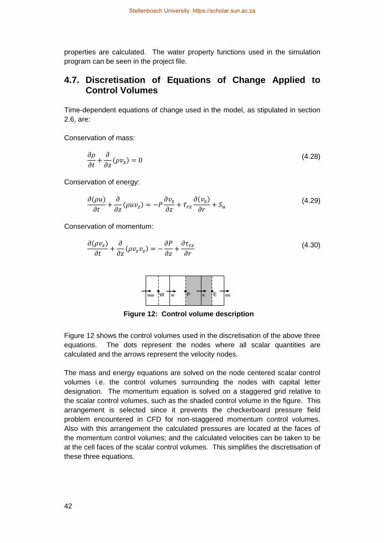
42

properties are calculated. The water property functions used in the simulation

program can be seen in the project file.

4.7. Discretisation of Equations of Change Applied to Control Volumes

Time-dependent equations of change used in the model, as stipulated in section

2.6, are:

Conservation of mass:

( )

(4.28)

Conservation of energy:

( )

( )

( )

(4.29)

Conservation of momentum:

( )

( )

(4.30)

Figure 12 shows the control volumes used in the discretisation of the above three

equations. The dots represent the nodes where all scalar quantities are

calculated and the arrows represent the velocity nodes.

The mass and energy equations are solved on the node centered scalar control

volumes i.e. the control volumes surrounding the nodes with capital letter

designation. The momentum equation is solved on a staggered grid relative to

the scalar control volumes, such as the shaded control volume in the figure. This

arrangement is selected since it prevents the checkerboard pressure field

problem encountered in CFD for non-staggered momentum control volumes.

Also with this arrangement the calculated pressures are located at the faces of

the momentum control volumes; and the calculated velocities can be taken to be

at the cell faces of the scalar control volumes. This simplifies the discretisation of

these three equations.

P E W w e ee ww

Figure 12: Control volume description


43

The three conservation equations are now developed into a discretised form that

is easily capable of being solved by a computer program. A fully implicit temporal

discretisation scheme is used. The fully implicit discretisation scheme is

unconditionally stable, thus larger time-step sizes, than for explicit methods, can

be used. A small time-step size is however used to ensure physically realistic

results. The fully implicit scheme uses new values only, thus it requires iteration

and in most cases under-relaxation is necessary.

The discretisation of the three conservation equations are to follow in the

particular order in which it was implemented within the simulation model; as can

be seen in the iteration script file, Itterate_UD_density_based.m, in Appendix C4.

4.7.1. Discretisation of the Conservation of Mass

The conservation of mass equation (4.28) is discretised to give an equation to

solve for the new densities based on a velocity or guessed velocity field.

Conservation of mass, repeated here for convenience:

( )

The conservation of mass is first integrated over a control volume and written in

terms of finite differences:

( )

[ ] [ ]

(4.31)

This expression is now formulated into a form to solve the density field based on

a given (or guessed) velocity field:

( )

[ ] [ ]

(4.32)

Define convection values (provides a shortened method of writing the equations)

as:

[ ] and [ ] (4.33)

where [ ] is the product of velocity and area at the western face of the

control volume and [ ] is the product - at the eastern face. Substitution gives:

( )

(4.34)


44

An upwind differencing scheme is selected for the face values of density, due to

its robustness when using a small number of control volumes. The development

of the final form of the discretised equation for the density follows the same

procedure as explained in section 2.6 for any general variable .

The final form is therefore:

(4.35)

where:

( )

( ) ( )

4.7.2. Discretisation of the Conservation of Energy

The conservation of energy equation (4.29) is discretised to give an equation to

solve for the new specific internal energy field based on the velocity field already

used above and the newly obtained density field.

Conservation of energy, repeated here for convenience:

( )

( )

( )

The conservation of energy is first integrated over a control volume and written in

terms of finite differences:

[( ) ( ) ]

[ ] [ ]

[( ) ( ) ]

(4.36)

Define convection values as:

[ ] and [ ] (4.37)

Substitution and rewriting yields:


45

[

]

[

]

[( ) ( ) ]

(4.38)

The source term is used to incorporate the heat transferred through the

tube walls and axial conduction in the gas. Also to accommodate programming

the pressure and shear stress components are included in the source term. Any

suitable discretisation method can now be used to represent the face values of

specific internal energy. Once again upwind differencing is selected for its

robustness and fundamental properties as discussed in section 2.6. Following

the procedure as outlined in section 2.6 gives:

(4.39)

where:

( )

( ) ( )

[( ) ( ) ]

4.7.3. Discretisation of the Conservation of Momentum

Before the momentum equation is discretised, the equation of state is used to

obtain updated values of all properties, including pressure, based on the newly

obtained density - and specific internal energy field.

The conservation of momentum equation (4.30) is discretised to give an equation

to solve for the new velocities based on the newly obtained density field and

properties (especially the pressure field).

Conservation of momentum, repeated here for convenience:

( )

( )

Integrating the conservation of momentum over the staggered momentum control

volume (shaded control volume in Figure 12) gives:


46

[( ) ( ) ]

[ ] ( ) [ ] ( )

( )

(4.40)

Define convection values as:

[ ] and [ ] (4.41)

Substitute and formulate this expression into a form to solve the velocities:

[

] ( ) ( ) ( )

[

] ( )

( )

(4.42)

Using upwind differencing as the discretisation scheme for the face velocities

gives:

( ) ( ) ( ) ( )

(4.43)

where:

( )

( ) ( )

( )

4.8. Algorithm for Simulating a Refrigeration Cycle

The flow is compressible, therefore the usual pressure based algorithms such as

SIMPLE (Semi-Implicit Method for Pressure-Linked Equations) are not well suited

to solving the flow equations. There is a strong link between density and

pressure in compressible flows. Figure 13 shows the density-based algorithm to

solve the conservation equations for each time-step. The simulation starts with

the initial conditions as described in section 4.2. The boundary conditions as set

out in section 4.3 are calculated at the start of each iteration (step 1). Each time-

step is solved in a similar fashion as with steady-state problems. To start the

simulation of the current time-step a velocity field for the scalar control volume


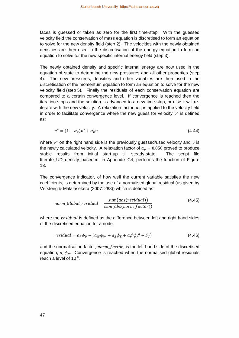
47

faces is guessed or taken as zero for the first time-step. With the guessed

velocity field the conservation of mass equation is discretised to form an equation

to solve for the new density field (step 2). The velocities with the newly obtained

densities are then used in the discretisation of the energy equation to form an

equation to solve for the new specific internal energy field (step 3).

The newly obtained density and specific internal energy are now used in the

equation of state to determine the new pressures and all other properties (step

4). The new pressures, densities and other variables are then used in the

discretisation of the momentum equation to form an equation to solve for the new

velocity field (step 5). Finally the residuals of each conservation equation are

compared to a certain convergence level. If convergence is reached then the

iteration stops and the solution is advanced to a new time-step, or else it will re-

iterate with the new velocity. A relaxation factor, , is applied to the velocity field

in order to facilitate convergence where the new guess for velocity is defined

as:

( ) (4.44)

where on the right hand side is the previously guessed/used velocity and is

the newly calculated velocity. A relaxation factor of proved to produce

stable results from initial start-up till steady-state. The script file

Itterate_UD_density_based.m, in Appendix C4, performs the function of Figure

13.

The convergence indicator, of how well the current variable satisfies the new

coefficients, is determined by the use of a normalised global residual (as given by

Versteeg & Malalasekera (2007: 288)) which is defined as:

( ( ))

( ( ))

(4.45)

where the is defined as the difference between left and right hand sides

of the discretised equation for a node:

(

) (4.46)

and the normalisation factor, , is the left hand side of the discretised

equation, . Convergence is reached when the normalised global residuals

reach a level of 10-8.


48

Start

STEP 2: Solve discretised mass conservation

equation to obtain new density

STEP 3: Solve discretised energy

conservation equation to obtain new specific

internal energy

STEP 4: Use equation of state modified to be

a function of density and specific internal

energy, to obtain new pressure and all other

scalar variables

STEP 5: Solve discretised momentum

conservation equation to obtain new velocities

Convergence?

Set

v* = v

Stop and advance

to new time-step

No

Yes

Initial guess for

velocity field, v*

v*, ρ

v*, ρ, u

v*, ρ, u, P,ϕ

v, ρ, u, P,ϕ

STEP 1: Calculate boundary conditions (mass

flowrate, specific internal energy and velocity)

v*

Figure 13: Density-based algorithm for solving compressible flow


49

5. REFRIGERATOR DESIGN

The system being designed is based on a small household refrigerator. The

system serves as a test unit to evaluate refrigeration performance at different

operating conditions, and to experimentally validate the simulation program

written in this thesis. There are many different routes to designing a refrigerator.

The design method explained here serves as an introductory method only.

5.1. Compressor Selection

To design a refrigerator an evaporator temperature is selected, an approximate

cooling load range is calculated or assumed, and the environment temperature

must be known. It was decided to build the system to be capable of reaching an

evaporator temperature of -10 . The compressor must be capable of producing

an outlet pressure that is equal or higher than the saturation pressure of the

refrigerant corresponding to the environmental temperature, in order to achieve

adequate heat rejection to the environment. Normal household refrigerators

have a rated cooling load of about 1 kW. The small EK6210CD CO2 refrigerant

compressor from Embraco (product data attached in Appendix D) is selected

since it is capable of working at these conditions with a rated cooling load of

700 W at the selected evaporation temperature of -10 . This rated cooling load

is deemed adequate for the test unit developed for this project.

5.2. Internal Volume of High Pressure Side

The volume of the high pressure (HP) side must be as low as possible in order to

ensure a high enough pressure and thus temperature for heat rejection. A

density limit for the HP side is placed by the compressor manufacturer (for

compressor safety), in the event of expansion device blockage (all refrigerant is

in the HP side only). The EK6210CD Embraco compressor specifies a system

with a maximum CO2 refrigerant charge of 500 and a maximum HP side density

of 0.65 /cm3 (Embraco, [S.a.]). It was selected to use 435 of CO2, which is

well below the 500 maximum specified.

Based on the mass of refrigerant used, the high side volume must be larger than:

(5.1)

The tubes used for the refrigerator are made of copper; most of them are thick-

walled in order to handle the high pressure requirements of the CO2 refrigerant

during operation. Table 4 shows the high pressure side tube details used to

manufacture the refrigerator.


50

To connect the different tubes to each other one can either solder them together

(a process called swaging of the tubes) or one can use Swagelok tube fittings.

Swagelok tube fittings offer easy assembly, disassembly and re-assembly of the

tubes therefore providing flexibility in changing the design if needed.

Table 4: Tube details of the high pressure side

Tubes used for the high pressure

side

Length, outer diameter,

thickness, pressure

rating

Inner

volume

(cm3)

Connecting tube between compressor

and gas cooler ( ) 2.15 m, 6.35 mm (1/4”),

0.91 mm, 119.9 bar 34.652

Gas cooler tube ( ) 19.7 m, 8 mm, 0.9 mm,

93.9 bar 594.757

Connecting tube between gas cooler

and internal heat exchanger ( ) 1 m, 6.35 mm, 0.91 mm,

119.9 bar 16.117

Internal heat exchanger inner tube

( )

2.5 m, 4.76 mm

(3/16”),0.61 mm, 105.9 bar 24.606

Connecting tube between inner tube

of IHX and capillary tube ( ) 0.45 m, 4.76 mm (3/16”),

0.61 mm, 105.9 bar 4.429

Total internal volume 674.558

In the simulation program the connection fittings are approximated by adding

cone shaped control volumes to account for momentum change at the changing

tube diameters and the extra volume added by the connection fittings. Therefore,

the high pressure side volume is marginally increased to a value of (as can be

seen in the simulation program initialise script in Appendix C2):

(5.2)

This value is larger than the lower limit set in equation (5.1), but not excessively

larger; thus it is an acceptable design.


51

𝐿𝑐𝑡1𝑝ℎ

𝐿𝑐𝑡 𝑝ℎ

𝑐𝑡 𝑃 𝑃𝑐𝑡𝑖𝑛

𝑃 𝑃𝑐𝑡𝑜𝑢𝑡 𝑐𝑡

𝐿𝑐𝑡

𝑁𝑐𝑡1𝑝ℎ

𝑁𝑐𝑡 𝑝ℎ

5.3. Capillary Tube Design using a Steady-State Capillary Tube Simulation Model

The low pressure (LP) side can now be considered in the design of a capillary

tube for the system. The capillary tube operates between inlet conditions at the

HP side and evaporator temperature needed at its outlet. It was selected to have

an evaporator saturation temperature of -10 .

The EK6210CD Embraco compressor has a rated cooling capacity of 700 W at

an evaporation temperature of -10 as shown in the product data attached in

Appendix D. The saturation pressure of CO2 at -10 is 26.487 bar. The

enthalpy entering the evaporator is equal to the enthalpy entering the capillary

tube since the adiabatic throttling process is isenthalpic. The enthalpy entering

the capillary tube is determined from the rated compressor discharge pressure of

85 bar and gas cooler return gas temperature of 32 . The enthalpy calculated

at this pressure and temperature is -217.84 kJ/kg. The compressor inlet

temperature from the test conditions is 32 . The enthalpy calculated at 32

and 26.487 bar is -20.24 kJ/kg. The mass flow rate corresponding to the rated

cooling capacity is therefore:

( )

(

) ⁄

(5.3)

A capillary tube now needs to be designed which can provide this mass flow rate

at the same operating conditions as shown in the product data from Embraco.

Figure 14 shows the steady-state capillary tube model which calculates the mass

flow rate based on a capillary tube length and inside diameter.

Figure 14: Steady-state capillary tube model


52

The inlet and outlet pressures and enthalpy of the capillary tube are as

mentioned above. Homogenous flow is assumed for the two-phase flow in the

simulation model. The steady-state simulation model is written to distinguish

between three different operating scenarios:

1) Single phase only (if and are both above the saturation pressure

at ). 2) Two-phase only (if and are both below the saturation pressure

at ).

3) Single phase for the first part and then two-phase for the rest of the length of the capillary tube (if is above - and is below the saturation

pressure at ).

The simulation model first determines the saturation pressure at and then

decides which scenario to follow. Depending on which scenario is encountered

the simulation domain is divided into a set number of control volumes of equal

pressure drop (and therefore variable length) for the corresponding phase.

Scenario three is encountered in the above test conditions; therefore the

simulation domain (capillary tube as shown in Figure 14) is divided into 100

control volumes in the single phase region with a pressure drop of:

1 ℎ

(5.4)

and 500 control volumes in the two-phase region with a pressure drop of:

ℎ

(5.5)

Each control volume is now assigned a pressure based on the constant pressure

drop per control volume along the capillary tube and the constant enthalpy as

given; thus properties for each control volume can now be calculated. To start

the simulation a capillary tube length and inner diameter is specified and a mass

flow rate is guessed. Based on the mass flow rate, inner diameter and the

pressure drop per control volume a corresponding length for each control volume

is calculated. The control volume lengths are then added together to calculate

the total length of the capillary tube. If the added length of the capillary tube is

more than the specified length, then the mass flow rate guessed is too small and

needs to be increased, otherwise it needs to be decreased.

The bisection method (Chapra, 2008: 122) is used to iteratively converge on the

correct mass flow rate. The steady-state capillary tube simulation model can be

seen in Appendix E. There are a few different capillary tube diameter options

available. From trial and error using the simulation program it was decided to


53

use the TC31 capillary tube with inner diameter of 0.031” (0.79 mm) and length of

3.5 m. It gives a mass flow rate of:

⁄ (5.6)

which is deemed close enough to the mass flow rate in equation (5.3).

5.4. Internal Volume of Low Pressure Side

Now that the volume of the high pressure side is known, the volume of the low

pressure (LP) side may be determined. The volume of the LP side depends on

the following two conditions: the evaporator temperature and the rated cooling

load of the compressor. The transient simulation program, as discussed in

section 4, is used to determine the low pressure side volume by successively

trying different volumes (tube lengths) until the one selected suits the conditions

mentioned above.

Table 5: Tube details of the low pressure side

Tubes used for the low pressure

side

Length, outer diameter,

thickness, pressure rating

Inner

volume

(cm3)

Evaporator tube ( ) 12.9 m, 8 mm,

0.9 mm, 93.9 bar 389.460

Connecting tube between evaporator

and internal heat exchanger ( )

0.93 m, 6.35 mm (1/4”),

0.91 mm, 119.9 bar 14.989

Internal heat exchanger outer tube

( )

2.5 m, 9.53 mm (3/8”),

0.91 mm, 79.6 bar 72.230

Connecting tube between internal

heat exchanger outer tube and

compressor ( )

0.35 m, 6.35 mm (1/4”),

0.91 mm, 119.9 bar 5.641

Total internal volume 482.320

Table 5 shows the low pressure side tube details obtained from the simulation

and used to manufacture the refrigerator. Again the simulation takes also into

account the added volume of the connection fittings between the tubes, therefore

the volume increases marginally to a value of (as can be seen in the simulation

program initialise script):


54

(5.7)

5.5. Heat Exchanger Designs

The design of a heat exchanger depends on the heat transfer rate needed and

the convection coefficients of the fluids exchanging the heat. For this project

tube-in-tube heat exchangers, with water in the outer tubes, are used for the gas

cooler and the evaporator. Water has a high convection heat transfer coefficient

and a high specific heat relative to air; therefore, it can absorb/reject more heat

per mass and at a faster rate than air. Also it is easy to control and measure its

temperature and mass flow rate; therefore it provides for a reliable method for

validation of heat transferred during experimentation.

Both evaporator and gas cooler are over designed to handle higher heat transfer

rates if needed; thus providing variable operating conditions for the refrigeration

system. The water inlet temperature and mass flow rate to the heat exchangers

can be varied; also sections of the heat exchangers can be included or excluded

in order to accomplish different cooling/heating loads. The refrigerator built thus

serves as a good experimental unit, capable of being tested thoroughly at

different operating conditions. Table 6 shows the details of the gas cooler - and

evaporator outer tubes.

Table 6: Details of the outer tubes of the heat exchangers

Tube lengths for the heat

exchanger outer tubes

Length, outer diameter of inner

tube, outer diameter of outer

tube, thickness of outer tube,

pressure rating of outer tube

Inner

volume

(cm3)

Gas cooler heat exchanger

outer tube

14 m, 8 mm, 15.88 mm (5/8”),

0.71 mm, 34.40 bar 1595.365

Evaporator heat exchanger

outer tube

12 m, 8 mm, 15.88 mm (5/8”),

0.71 mm, 34.40 bar 1367.456


56

6. EXPERIMENTAL SETUP

The refrigerator system shown in Figure 15 is now set up with experimental

equipment necessary to measure its performance. First the calibration method

for the thermocouples used is explained, then the total experimental setup is

shown, and finally the experimental test procedure is discussed.

6.1. Thermocouple Calibration

The 20 T-type thermocouples used for the experiment were calibrated using a

platinum resistance thermometer and a Fluke field metrology well system

(manufacturer: model nr: 9142, serial nr: B29291) The Fluke system generates

the desired calibration temperature, by heating or cooling the metal bar insert it

uses, and measures the resistance of the thermometer. The platinum resistance

thermometer details are:

Manufacturer: ISOTECH

Model number: 935-14-72

Serial number: 191069

The thermometer was calibrated at Rapid Instrumentation CC (a member of the

South African National Accreditation System (SANAS) with Accredited

Laboratory Number 366). The calibration certificate number is: RAP15738.

The procedure for calibration is as follows: a number of thermocouples are

inserted into a metal bar and then the bar is inserted in the Fluke system. A

temperature set point is set for the Fluke system and then allowed sufficient time

to reach steady-state. Once the Fluke system reaches steady-state (the Ohm

reading of the thermometer remains constant), the Agilent Data Logger scan is

started and it is first confirmed that the corresponding thermocouples have

indeed reached state-state; only then is the scan restarted to store the steady-

state measured temperatures of the corresponding thermocouples.

Temperatures are recorded every 5 s for a period of about 4 minutes. At the

same time the Ohm reading for the platinum resistance thermometer is recorded

manually into a spread sheet from which the corresponding true temperature is

calculated. It was deemed sufficient for the refrigerator experiment to have

calibration points from -10 to 100 at 10 intervals. Average values for

each temperature point are then calculated for each thermocouple. The average

measured values are then plotted versus the true values, as shown in Figure 16

for thermocouple 1. The remaining thermocouples all have a good correlation

coefficient to their straight trend lines; therefore, it was decided for brevity not to

show all the thermocouple calibration plots here (Appendix F provides a table of

all the calibration equations and their correlation coefficients).


57

Figure 16: Thermocouple 1 - calibration curve

6.2. Experimental System Layout

The experimental setup, shown in Figure 17, consists of the refrigeration system,

as shown in Figure 15, with 20 T-type thermocouples, 2 pressure gauges, a

control unit for the compressor, a water container, a water pump, a water chiller,

a laptop, a data logger and a video camera (CAT B-15 smartphone).

Tt = 0.99942370 Tm - 0.49370601 R² = 0.99999841

-20

0

20

40

60

80

100

120

-20 0 20 40 60 80 100 120

Tru

e t

em

pe

ratu

re, T

t [

]

Measured temperature, Tm [ ]

Submersible

water pump

Data

logger

Water

chiller

Water

container

Laptop

Refrigeration

system

Gas cooler and

evaporator

outlet water

Video camera

to record

pressure

Figure 17: Experimental system


59

The experimental recording part may now commence as follows:

First record a set of data to keep as reference of the initial conditions for

the experiment. Usually around 3 to 5 minutes of data.

Place the video camera (CAT B-15 smartphone) at the desired location

and start to record the pressure gauges.

Start recording data on the laptop and then switch on the refrigerator.

Observe the recording time when the compressor turns on. Usually

around 52 seconds after switching the switch on.

Record data until all temperatures have reached a sufficiently stable

value.

Switch off the data logger and the compressor. Test is complete.


61

7.2. Boundary Conditions and External Heat Exchangers

The boundary conditions, enforced by the compressor, for the simulation domain

are as discussed in section 4.3; with a step-input compressor speed at t = 0 s of

N = 2400 rpm, a constant compressor volumetric efficiency of 0.954 and a

constant isentropic efficiency of 0.716.

The external heat exchangers (gas cooler and evaporator) contain water flowing

in the outer tubes at a mass flow rate of 0.050 k /s, in a counter flow direction in

relation to the CO2 refrigerant flow, and at an inlet temperature of 25 .

7.3. Grid Independence

A grid independence study is done, as shown here in Figure 20, for the pressure

distribution at 150 ms simulation time. It was decided to use the pressure

distribution as an indication of grid independence, since all fluid properties are

dependent mainly on the operating pressure in the system. The pressure

distribution for the different grid sizes show that further grid refinement produces

no remarkable difference; thus grid independence has been achieved. Based on

this study and in the interest of producing results that are reasonably accurate, in

the least amount of time, it was elected to use a grid size of i.e. use

1390 control volumes.

Figure 20: Pressure distribution at 150 ms for grid independence study

0 5 10 15 20 25 30 35 40 456200

6300

6400

6500

6600

6700

6800

N

tot=1030

Ntot

=1390

Ntot

=1560

Length, z [m]

Pre

ssure

, P

[kP

a]


62

7.4. Simulation Domain Geometry Properties

From the grid independence study it was chosen to use a total number of 1390

control volumes for the simulation domain. The excerpt below, from the initialise

scrip file in Appendix C2, shows the number of control volumes used for the

different sections of the simulation domain.

%Form the control volumes of the whole solution domain.

N_comp_gc = 52; %Number of cv's for the connecting tube

%between outlet of compressor and inlet of

%gas cooler.

N_tr1 = 1; %Number of cv's for transition between

%comp_gc tube and gas cooler tube.

N_gc = 400; %Number of cv's for the gas cooler.

N_tr2 = 1; %Number of cv's for transition between gas

%cooler tube and gc_IHX tube

N_gc_IHX = 66; %Number of cv's between outlet of gas cooler

%and IHX.

N_tr3 = 1; %Number of cv's for transition between

%gc_IHX tube and IHX tube

N_IHX = 120; %Number of cv's for the Internal Heat

%Exchanger (IHX) inner tube.

N_tr4 = 1; %Number of cv's for transition between IHX

%tube and IHX_ct tube

N_IHX_ct = 24; %Number of cv's for the connecting tube

%between IHX and Capillary tube.

N_tr5 = 2; %Transition between IHX_ct tube and

%capillary tube

N_ct = 230; %Number of cv's for the Capillary Tube.

N_tr6 = 2; %Transition between capillary tube and

%evaporator tube

N_ev = 300; %Number of cv's for the Evaporator.

N_tr7 = 1; %Transition between evaporator tube and

%ev_IHX tube

N_ev_IHX = 40; %Number of cv's for the connecting tube

%between outlet of Evaporator and IHX.

N_tr8 = 3; %Transition between ev_IHX tube and IHX tube

%N_IHX = 120; %Number of cv's used for outer tube of IHX

N_tr9 = 3; %Transition between IHX tube and IHX_comp

%tube

N_IHX_comp = 23;%Number of cv's for the connecting tube

%between the IHX outlet and compressor

%inlet.

Figure 21 shows the control volume lengths for the different sections. A stretch

ratio is applied to the different tube sections i.e. variable control volume lengths

are used. The minimum control volume length is decided as 15 mm, which is

due to transition pieces used between tube sections. The stretch ratio is kept

close to a value of one in order to have a good aspect ratio from one control


71

The slight undershoots and overshoots seen at the transition of tubes (deemed

acceptable as is) can be further reduced by refining the mesh locally or by

implementing a second-order upwind differencing scheme instead of the first-

order upwind differencing scheme currently used.

9. EXPERIMENTAL VERSUS SIMULATION RESULTS

In this section the experimental results are compared to the simulation results.

The experimental results used are from one of three experiments done at the

same conditions to confirm repeatability. The experimental temperatures were

measured by tightly tying the thermocouples to the outside of the copper tubes.

The simulation temperatures refer to the temperature of the CO2 flowing inside

the tubes.

The simulation results shown in section 8, and this section, are for the case

where the initial conditions are 25 , water inlet temperature to the heat

exchangers are also 25 , the water mass flow rate is 0.050 k /s, and the

cooling section of the gas cooler is 14 m long and starts at a distance z = 2.17 m

from the simulation domain inlet. The experimental refrigerator was however

built with the gas cooler cooling section starting at z = 7.73 m. It is expected that

this discrepancy would not cause much of a difference to the actual operation of

the refrigerator. Furthermore, it was not possible to obtain the wanted 0.050 kg/s

water mass flow rate for the experiment; consequently, the average mass flow

rate measured for the evaporator and gas cooler outer tubes was 0.045548 k /s.

Figure 30 shows a comparison of the pressure development predicted by the

simulation and what was recorded in the experiment. The initial pressures of the

experiment and simulation are 5900 kPa and 6434 kPa, respectively. The

saturation temperature for CO2 at 5900 kPa is 21.25 . This confirms the initial

suspicion that the CO2 (low conductivity) has not yet reached the new

experimental ambient temperature from the previous night’s colder temperature.

Furthermore, from the figure it is seen that the simulation develops relatively

faster than the experiment does, but reaches a steady-state that is relatively

close to the experiment. The quick response of pressure is due to the use of a

constant isentropic efficiency from start-up and the assumption that the

compressor is at full speed from t = 0 s. The water being as close as possible to

the compressor outlet dampens the pressure by absorbing heat, thus ensuring

that the pressure doesn’t reach hazardously high levels. The compressor is a

hermetically sealed unit that is intentionally cooled during operation; thus, cooling

the gas while it is being compressed. The efficiency would thus be a changing

function that is dependent on the transient operating conditions and cooling. It is

thus recommended to rather use an isothermal (non-adiabatic) efficiency model


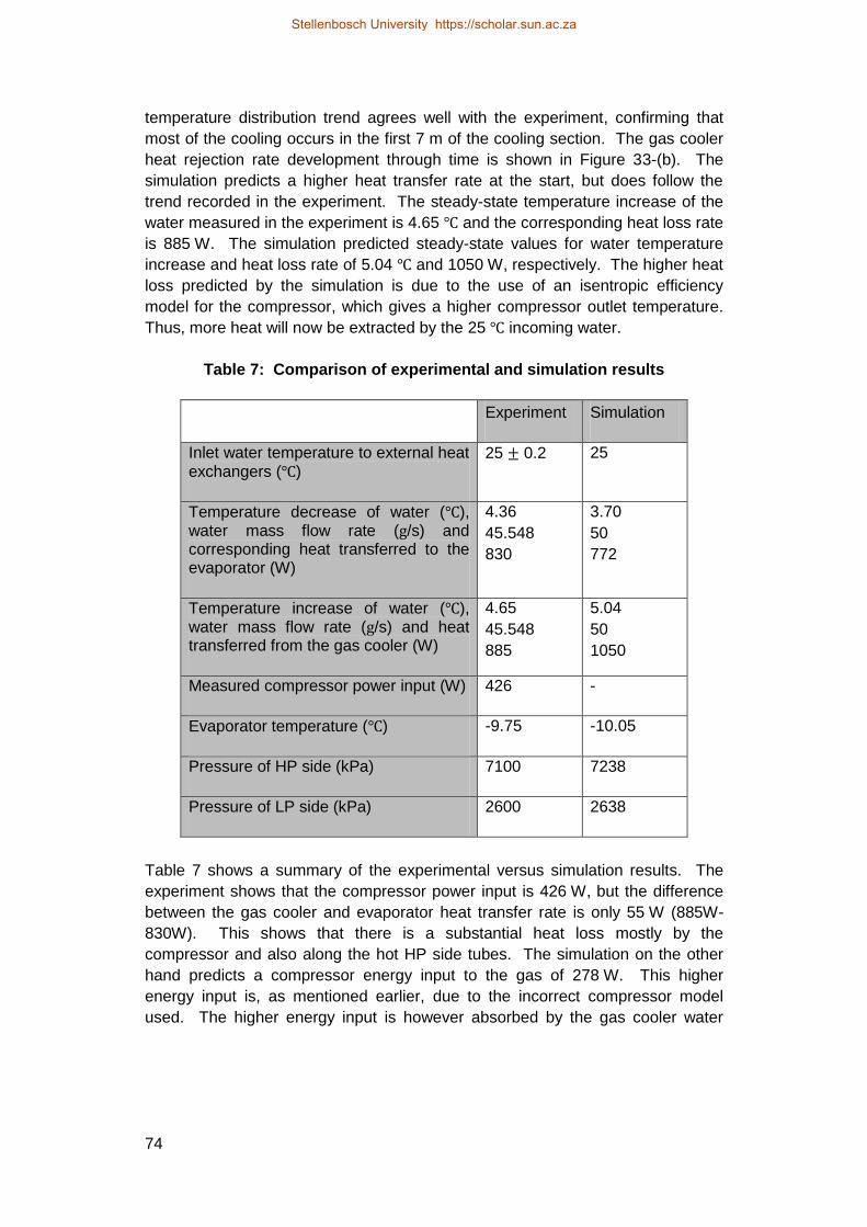
74

temperature distribution trend agrees well with the experiment, confirming that

most of the cooling occurs in the first 7 m of the cooling section. The gas cooler

heat rejection rate development through time is shown in Figure 33-(b). The

simulation predicts a higher heat transfer rate at the start, but does follow the

trend recorded in the experiment. The steady-state temperature increase of the

water measured in the experiment is 4.65 and the corresponding heat loss rate

is 885 W. The simulation predicted steady-state values for water temperature

increase and heat loss rate of 5.04 and 1050 W, respectively. The higher heat

loss predicted by the simulation is due to the use of an isentropic efficiency

model for the compressor, which gives a higher compressor outlet temperature.

Thus, more heat will now be extracted by the 25 incoming water.

Table 7: Comparison of experimental and simulation results

Experiment Simulation

Inlet water temperature to external heat

exchangers ( ) 25 0.2 25

Temperature decrease of water ( ), water mass flow rate ( /s) and corresponding heat transferred to the evaporator (W)

4.36

45.548

830

3.70

50

772

Temperature increase of water ( ), water mass flow rate ( /s) and heat transferred from the gas cooler (W)

4.65

45.548

885

5.04

50

1050

Measured compressor power input (W) 426 -

Evaporator temperature ( ) -9.75 -10.05

Pressure of HP side (kPa) 7100 7238

Pressure of LP side (kPa) 2600 2638

Table 7 shows a summary of the experimental versus simulation results. The

experiment shows that the compressor power input is 426 W, but the difference

between the gas cooler and evaporator heat transfer rate is only 55 W (885W-

830W). This shows that there is a substantial heat loss mostly by the

compressor and also along the hot HP side tubes. The simulation on the other

hand predicts a compressor energy input to the gas of 278 W. This higher

energy input is, as mentioned earlier, due to the incorrect compressor model

used. The higher energy input is however absorbed by the gas cooler water


75

which is 165 W more than in the experiment. This counters the effects of the

isentropic compressor model used and explains why the simulation predicted

pressures that are relatively close to the experimental pressures. It was however

found that if the gas cooler cooling section was moved further away from the

compressor outlet, then the pressures reached by the simulation are higher than

the experiment. The water cooling section being further away from the

compressor amplifies the effects of the incorrect compressor model used. Also

the simulation model does not account for axial heat conduction in the copper

connecting tubes.

From these results it is evident that a non-adiabatic transient compressor model

should be adopted instead of an isentropic compressor model. Due to the

inaccurate compressor model used it was decided not to include simulation

results for other operating cases, since they would have no further meaning. The

results shown by the simulation in this report are nonetheless a confirmation that

the simulation model predicts operation within the refrigerator fairly well; and

would be more so, if the boundary conditions (compressor model) employed

were better. Developing a non-adiabatic transient compressor model is outside

the scope of this project.


76

10. OTHER EXPERIMENTAL RESULTS

Table 8 shows the experimental results for four different operating conditions.

Note that the ambient temperature is also maintained at the same temperature as

the inlet water to the external heat exchangers. The results show an increase of

evaporator temperature with increasing evaporator external water inlet

temperature used. From the results it is evident that the refrigerator built was

successful in reaching an evaporator temperature close to -10 .

The system’s measured COP is between 1.86 and 2.12. Additionally, the results

show that only 11 to 14 % of the compressor input power is transferred to the gas

(determined by the difference between gas cooler and evaporator heat transfer

rates measured), while the rest is lost to the environment. The compressor shell

temperature was also recorded during experiments. It showed an increase from

start-up to steady-state, meaning that the compressor body also absorbs heat

from the gas during transient conditions. This confirms the need for using a non-

adiabatic transient compressor model for the simulation.

Table 8: Steady-state experimental results for different water inlet

temperatures

Inlet water temperature to external

heat exchangers ( )

20 22.5 25 27.5

Temperature decrease of water

( ), water mass flow rate ( /s) and

corresponding heat transferred to

the evaporator (W)

4.55

44.675

851

4.55

44.869

844

4.36

45.548

830

4.35

45.554

828

Temperature increase of water ( ),

water mass flow rate ( /s) and heat

transferred from the gas cooler (W)

4.8

44.777

898

4.72

45.161

891

4.65

45.548

885

4.65

45.752

889

Measured compressor power input

(W)

401 416 426 444

Evaporator temperature ( ) -11.90 -10.70 -9.75 -8.01

Pressure of HP side (kPa) 6800 6950 7100 7800

Pressure of LP side (kPa) 2480 2550 2600 2750

Coefficient of performance 2.12 2.03 1.95 1.86


77

11. DISCUSSION OF RESULTS

The results obtained by the simulation model are dependent on the compressor

model used, since this provides the boundary conditions to the simulation model.

The simulation predicts a compressor outlet temperature which is higher than in

the experiment, as shown in Figure 31. Also, the experimental results in section

10 show a remarkable heat loss by the compressor, and it was mentioned that

the compressor body absorbed heat during the transient process. From the

above it is confirmed that the use of a constant isentropic efficiency compressor

model (determined from one steady-state point) for the transient simulation

model is not appropriate. Therefore, the results shown for the simulation are

slightly in error; nonetheless, they still prove that the simulation behaves as

expected and confirm that this simulation model can be used for refrigerator

designs. The development of a non-adiabatic transient compressor model is

outside the scope of this project.

The transient simulation results in section 8 shows how the refrigeration system

develops through time. They provide a reasonably accurate description of what

occurs within the refrigeration system as the system transitions from standstill

through to steady-state conditions. The simulation gives results that correlate

well with actual experimental results and expected behaviour.

The pressure wave travels through the domain at the speed of sound, for that

corresponding pressure, as shown in Figure 22. The operation of the capillary

tube is confirmed in these same graphs by the pressure difference it causes

between the low and high pressure side. The constant temperature sections, at

about 30 m, shown in the bottom two graphs in Figure 23 confirm that the

simulation predicts real life constant temperature (and constant pressure) phase

change processes, as encountered in an evaporator. Note there is a small

temperature drop with frictional pressure drop here, but it is so small that it’s

virtually “constant”. Heat addition causes phase change from two-phase to

saturated gas at a constant temperature, and subsequent heat addition causes a

temperature rise.

The velocity graphs in Figure 24 show the high velocity encountered in the

capillary tube as expected. Also, it shows how the velocity increases towards its

outlet; this is due to a decrease in density along the capillary tube. The mass

flow rate graphs in Figure 25 show how the system reaches a steady-state mass

flow rate. At the start the compressor has a high mass flow rate due to the high

density of the saturated vapour at inlet. The mass flow rate decreases now with

decreasing density of the super-heated vapour (at lower pressure) at the inlet; up

until the refrigeration system reaches steady-state where the inlet (or inlet

density) and outlet conditions of the compressor remain constant. Steady-state


78

is achieved since the compressor performance is now in equilibrium with the

refrigeration system.

The steady-state pressure drop through the sections of the refrigerator shown in

Figure 29 confirms the “text-book” assumptions that the LP and HP side could be

approximated by constant pressure processes. The capillary tube pressure drop

has a slight curve indicating an increase in pressure drop towards the end of the

capillary tube; this is due to the increasing friction brought by the higher velocities

encountered towards the end of the capillary tube.

The results shown in section 9 confirm that the simulation model correlated well

with the experimental system; thus the simulation model is successful. The

evaporator temperature, LP and HP pressure achieved by the simulation agrees

well with the experiment. The heat transfer rates of the evaporator and gas

cooler show trends similar to the experiment and reach steady-state values that

are close to the experiment.


79

12. CONCLUSIONS AND RECOMMENDATIONS FOR FUTURE WORK

Refrigeration has become a highly essential part of modern day living. Recent

abandonment of synthetic refrigerants, due to their damaging effects on the

environment, has renewed interest in using CO2 as refrigerant. CO2 is a natural

gas with no ozone depletion potential and a low global warming potential. The

need to obtain a better understanding of CO2 refrigeration cycles and to design

CO2 refrigerators with a higher COP has led to the development of a transient

simulation model for CO2 refrigerators.

For the development of the transient simulation model a literature study was

done covering aspects such as the theoretical vapour-compression refrigeration

cycle, the CO2 transcritical refrigeration cycle, properties of an ideal refrigerant,

properties of CO2 as refrigerant, and finally the use of the control volume method.

Furthermore, methods for determining the state of CO2 in a control volume were

developed, which are based on the use of the real gas equation of state for CO2

from Span and Wagner (1996). These methods cover saturated, single phase

and two-phase property determination at a given density and specific internal

energy. Finally, assumptions, geometry, boundary conditions and conservation

equations (employing the 1D-CFD approach) were defined for the transient

simulation model. Lastly, a density-based algorithm to solve the compressible

flow equations for the simulation model was developed. The transient simulation

model was now complete.

To validate the transient simulation model, a CO2 refrigerator had to be built. For

this reason a CO2 refrigerator design procedure was developed and used to

obtain the design of the experimental refrigerator. The design procedure

involved the use of a steady-state capillary tube simulation model to obtain the

design of the capillary tube, and used the transient simulation model to validate

the design of the entire system.

The refrigerator built was successful in reaching the evaporator design

temperature of -10 for a cooling load close to the rated cooling load. This

proves that the simulation model may be used to design CO2 refrigerators.

Experimentation was conducted successfully for different water inlet

temperatures to the external heat exchangers (gas cooler and evaporator). The

experimentation focussed on capturing the transient behaviour of the system

from start-up till steady-state conditions.

The simulation results all showed a good correlation to the experimental results

and provided valuable insight into the processes occurring within the refrigerator.

It was found that the constant isentropic efficiency compressor model used for

the simulation over predicted energy input to the gas; thus, leading to higher


80

compressor outlet temperatures than the experiment and subsequently also a

higher heat removal rate in the gas cooler. The experimental results show that

there is a substantial heat loss by the compressor; therefore, confirming the need

for using a non-adiabatic transient compressor model in the simulation. This was

however outside the scope of this project.

In conclusion, the transient simulation model of the CO2 refrigerator runs stably

on its own and predicts real life operation fairly accurately; thus, it shows promise

in being a valuable tool for designing CO2 refrigerators if a non-adiabatic transient

compressor model is developed. It is recommended for future work to use the

experimental refrigerator built to test the system at different operating conditions

(different ambient temperatures and different heating or cooling water

temperatures to the heat exchangers) and thus ultimately developing a non-

adiabatic transient compressor model.


81

13. REFERENCES

Aljuwayhel N.F., Nellis G.F., Klein S.A. 2005. Parametric and Internal Study of

the Vortex Tube Using a CFD Model. International Journal of Refrigeration 28:

442-550.

ASHRAE. 2001. ASHRAE Handbook-Fundamentals, Chapter 19.

Barthel C., Götz T. 2012. The overall worldwide saving potential from domestic

refrigerators and freezers. [On-line]. Available:

http://www.bigee.net/media/filer_public/2012/12/04/bigee_doc_2_refrigerators_fr

eezers_worldwide_potential_20121130.pdf [2015, August 7].

Behera U., Paul P.J., Kasthurirengan S., Karunanithi R., Ram S.N., Dinesh K.,

Jacob S. 2005. CFD Analysis and Experimental Investigations towards

Optimizing the Parameters of Ranque-Hilsch Vortex Tube. International Journal

of Heat and Mass Transfer 48: 1961-1973.

Briley, G.C. 2004. A History of Refrigeration. ASHRAE Journal, November

2004: 531-534.

Çengel Y.A., Boles M. A. 2007. Thermodynamics: An Engineering Approach. 6

ed. New York: McGraw-Hill.

Chapra S.C., 2008. Applied Numerical Methods with MATLAB for Engineers

and Scientists. 2 ed. New York: McGraw-Hill.

Eiamsa-ard S., Promvonge P. 2007. Review of Ranque-Hilsh Effects in Vortex

Tubes. Renewable and Sustainable Energy Reviews 12: 1822-1842.

Embraco. [S.a.]. Carbon Dioxide (R744) EK6210CD Compressor Application

Manual.

Fenghour A., Wakeham W.A., Vesovic V. 1998. The Viscosity of Carbon

Dioxide. J. Phys. Chem. Ref. Data, Vol. 27, No. 1: 31-44.

Gupta U.S., Joshi M.K., Pawar C.B. 2012. Experimental Performance

Evaluation of Counter Flow Vortex Tube. Journal of Environmental Research

and Development 7 No.1A: 496-502.

Hamdan M.O., Alsayyed B., Elnajjar E. 2013. Nozzle Parameters Affecting

Vortex Tube Energy Separation Performance. Heat Mass Transfer 49: 533-541.


82

History of Refrigeration. 2015. [On-line]. Available:

http://www.peakmechanical.ca/history-of-refrigeration.html [2015, July 9].

Jenson J.B. 2008. Optimal Operation of Refrigeration Cycles. PhD Thesis.

Norway: Norwegian University of Science and Technology.

Jordan R.C., Priester G.B. 1949. Refrigeration and Air Conditioning. London:

Constable and Company, LTD.

Keysight Technologies. 2015. 34970A Data Acquisition/Data Logger Switch

Unit. [On-line]. Available: http://www.keysight.com/en/pd-

1000001313:epsg:pro-pn-34970A/data-acquisition-data-logger-switch-

unit?&cc=ZA&lc=eng [2015, November 9].

Kröger D.G. 1998. Air-cooled Heat Exchangers and Cooling Towers. Thermal-

flow Performance Evaluation and Design. Stellenbosch: Stellenbosch University.

Marsch R.W., Olivo C.T. 1979. Basics of Refrigeration. 2 ed. New York: Van

Nostrand Reinhold Company.

Mohiuddin M., Elbel S. 2014. A Fresh Look at Vortex Tubes used as Expansion

Device in Vapour Compression Systems. International Refrigeration and Air

Conditioning Conference. Purdue: Purdue University.

Nellis G.F., Klein S.A. 2002. The Application of Vortex Tubes to Refrigeration

Cycles. International Refrigeration and Air Conditioning Conference. Purdue:

Purdue University.

Nimbalkar S.U., Muller M.R. 2009. An Experimental Investigation of the

Optimum Geometry for the Cold End Orifice of a Vortex Tube. Applied Thermal

Engineering 29: 509-514.

Patankar, S.V. 1980. Numerical Heat Transfer and Fluid Flow. Series in

computational methods in mechanics and thermal sciences. Washington:

Hemisphere Publishing Corporation.

Promvonge P., Eiamsa-ard S. 2005. Investigation on the Vortex Thermal

Separation in a Vortex Tube Refrigerator. ScienceAsia 31: 215-223.

Saidi M.H., Valipour M.S. 2003. Experimental Modeling of Vortex Tube

Refrigerator. Applied Thermal Engineering 23: 1971-1980.

Sarkar J. 2009. Cycle Parameter Optimization of Vortex Tube Expansion

Transcritical CO2 System. Varanasi: BHU.


83

Sarkar J. 2010. Review on Cycle Modifications of Transcritical CO2

Refrigeration and Heat Pump Systems. Varanasi: BHU.

Scalabrin G., Marchi P., Finezzo F., Span R. 2006. A Reference Multiparameter

Thermal Conductivity Equation for Carbon Dioxide with an Optimized Functional

Form. J. Phys. Chem. Ref. Data, Vol. 35, No. 4: 1549-1575.

Singh P.K., Tathgir R.G., Gangacharyulu D., Grewal G.S. 2004. An

Experimental Performance Evaluation of Vortex Tube. IE (I) Journal – MC 84:

149-153.

Span R., Wagner W. 1996. A New Equation of State for Carbon Dioxide

Covering the Fluid Region from the Triple-Point Temperature to 1100 K at

Pressures up to 800 MPa. J. Phys. Chem. Ref. Data, Vol. 25, No. 6: 1509-1596.

Susort N.A. 2012. Refrigeration Cycle CO2. Specialization project 2012 TKP

4550. Norway: Norwegian University of Science and Technology.

The Montreal Protocol on Substances that deplete the ozone layer. 1987. [On-

line]. Available: http://ozone.unep.org/en/montreal_protocol.php [2015,August

5].

Trott A.R., Welch T.C. Refrigeration and Air-Conditioning. 3 ed. Butter-

Heinemann: Woburn.

Vera, G.D. 2010. The Ranque-Hilsch Vortex Tube. [On-line]. Available:

http://www.me.berkeley.edu/~gtdevera/notes/vortextube.pdf [2015, July 8].

Versteeg H.K., Malalasekera W. 2007. An Introduction to Computational Fluid

Dynamics. The Finite Volume Method. 2 ed. Harlow: Pearson Education

Limited.

Wagner W., Pruß A. 2002. The IAPWS Formulation 1995 for the

Thermodynamic Properties of Ordinary Water Substance for General and

Scientific Use. J. Phys. Chem. Ref. Data, Vol. 31, No. 2: 387-535.

Yilmaz M., Kaya M., Karagoz S. Erdogan S. 2009. A Review on Design Criteria

for Vortex Tubes. Heat Mass Transfer 45: 613-632.

Zhang W.J., Zhang C.L., Ding G.L. 2008. On Three Forms of Momentum

Equation in Transient Modeling of Residential Refrigeration Systems.

International Journal of Refrigeration 32 (2009): 938-944.


84

APPENDIX A: SAMPLE CALCULATIONS

Sample calculations for values stated in the report.

A1: Sample Calculations for an Ideal CO2 Refrigeration Cycle with an Ideal Work Recovering Expansion Device

The sample calculations shown here are for section 2.4.3. The calculations show

how the coefficient of performance improves due to the addition of an ideal work

recovering expansion device. The operating conditions for the cycle are as

mentioned in ASHRAE-Fundamentals (2001: 19.8). The conditions are 258 K

evaporation temperature and 303 K condensing temperature. The inlet of the

expansion device is at saturated liquid and the inlet of the compressor is at

saturated vapour. There is no pressure drop through the tubes.

The cycle performance is evaluated for a cooling load of 1 kW. Calculations for

the values stated in table 2 are shown below.

Evaporator pressure is:

Condenser pressure:

Compression ratio:

Net refrigerating effect:

s @

= -1.40 kJ/k

@

= -221.62 kJ/k

( )

kJ/k


85

Refrigerant circulated:

Specific volume of suction gas:

⁄

⁄

Compressor displacement rate:

⁄

Compressor power needed to compress the vapour:

s @

= -0.8145 kJ/k

@

= -70.48 kJ/k

@

= -21.40 kJ/k

( )

( ( ))

Power recovered from isentropic expansion and used to aid the compression

process:

s @

= -1.40 kJ/k

@

= -203.73 kJ/ k

@

= -221.62 kJ/ k


86

( )

( ( ))

Compressor power consumption with the work recovery:

Coefficient of performance:

Compressor discharge temperature:

@

K = K


87

APPENDIX B: Property Function Codes for CO2

The following MATLAB program codes are specifically written to calculate the

properties of CO2 for the control volume method implemented in the refrigeration

simulation model, as discussed in section 3. It is based on the use of the real

gas equation of Span and Wagner (1996) to calculate the properties of CO2.

B1: Function to Calculate the Single Phase Properties at a Given Density and Temperature

%CO2_Property.m is a script file written to calculate all derivatives and values

%needed in the equation of Span and Wagner (1996) to calculate the thermodynamic

%properties of CO2 i.e. it is a direct implementation of Span and Wagner’s

%equation of %state. The .mat file containing all variables,

%CO2_Property_Workspace.mat, is called %before-hand to import all variables needed

%in the Span and Wagner equation.

%Apply special treatment to avoid using rho=rho_c, for which the equations would

%give meaningless results i.e. properties at the critical density are taken in the

%limit close enough to the actual critical density.

if abs(rho-rho_c)<1e-13 %i.e. avoid critical density

rho=rho_c+1e-13;

end

delta = rho/rho_c; %Reduced density

tau = T_c/T; %Inverse of reduced temperature

%Following Table 28 in Span and Wagner to calculate the ideal-gas part of the

%Helmholtz energy Phi_o

%Initialize variables

%Ideal-gas part of the dimensionless Helmholtz function Phi_o

Phi_o = log(delta)+a_o(1)+a_o(2)*tau+a_o(3)*log(tau);

%1st and 2nd derivative of the dimensionless Helmholtz function Phi_o w.r.t. tau

Phi_o_tau1 = a_o(2)+a_o(3)/tau; Phi_o_tau2 = -a_o(3)/tau^2;

%Calculate and update variables

for p = 4:8

Phi_o = Phi_o + a_o(p)*log(1-exp(-tau*theta_o(p)));

Phi_o_tau1 = Phi_o_tau1+a_o(p)*theta_o(p)*((1-exp(-tau*theta_o(p)))^(-1)-1);

Phi_o_tau2 = Phi_o_tau2 - a_o(p)*(theta_o(p)^2)*exp(-tau*theta_o(p))*...

((1-exp(-tau*theta_o(p)))^(-2));

end

%1st and 2nd derivative of the dimensionless Helmholtz function Phi_o w.r.t. delta

Phi_o_delta1 = 1/delta;

Phi_o_delta2 = -1/delta^2;

%Derivative of the dimensionless Helmholtz function Phi_o w.r.t. delta and tau

Phi_o_delta_tau = 0;

%Following Table 32 in Span and Wagner to calculate the residual part of

%the Helmholtz energy Phi_r

for p = 1:3

THETA(p,1) = (1-tau)+A__S4(p)*((delta-1)^2)^(1/(2*beta_S4(p)));

DELTA(p,1) = THETA(p)^2 + B__S4(p)*((delta-1)^2)^a_S4(p);

PSI(p,1) = exp(-C__S4(p)*(delta-1)^2-D__S4(p)*(tau-1)^2);

%Derivatives of the exponential function

%1st and 2nd derivative w.r.t. delta

PSI_delta1(p,1) = -2*C__S4(p)*(delta-1)*PSI(p);

PSI_delta2(p,1) = (2*C__S4(p)*(delta-1)^2-1)*2*C__S4(p)*PSI(p);

%1st and 2nd derivative w.r.t. tau

PSI_tau1(p,1) = -2*D__S4(p)*(tau-1)*PSI(p);

PSI_tau2(p,1) = (2*D__S4(p)*(tau-1)^2-1)*2*D__S4(p)*PSI(p);

%Derivative w.r.t. delta and tau

PSI_delta_tau(p,1) = 4*C__S4(p)*D__S4(p)*(delta-1)*(tau-1)*PSI(p);


88

%------------------------------

DELTA_delta1(p,1) = (delta-1)*(A__S4(p)*THETA(p)*(2/beta_S4(p))*((delta-1)^2)^...

(1/(2*beta_S4(p))-1)+2*B__S4(p)*a_S4(p)*((delta-1)^2)^(a_S4(p)-

1));

part1 = 4*B__S4(p)*a_S4(p)*(a_S4(p)-1)*((delta-1)^2)^(a_S4(p)-2)+...

2*A__S4(p)^2*(1/beta_S4(p))^2*(((delta-1)^2)^(1/(2*beta_S4(p))-1))^2+...

A__S4(p)*THETA(p)*(4/beta_S4(p))*(1/(2*beta_S4(p))-1)*...

((delta-1)^2)^(1/(2*beta_S4(p))-2);

DELTA_delta2(p,1) = 1/(delta-1)*DELTA_delta1(p)+(delta-1)^2*part1;

%-------------------------------

%Derivatives of the distance function DELTA^bi

%1st and 2nd derivative w.r.t. delta

DELTAbi_delta1(p,1) = b_S4(p)*DELTA(p)^(b_S4(p)-1)*DELTA_delta1(p);

DELTAbi_delta2(p,1) = b_S4(p)*(DELTA(p)^(b_S4(p)-1)*DELTA_delta2(p)+...

(b_S4(p)-1)*DELTA(p)^(b_S4(p)-2)*DELTA_delta1(p)^2);

%1st and 2nd derivative w.r.t. tau

DELTAbi_tau1(p,1) = -2*THETA(p)*b_S4(p)*DELTA(p)^(b_S4(p)-1);

DELTAbi_tau2(p,1) = 2*b_S4(p)*DELTA(p)^(b_S4(p)-1)+4*THETA(p)^2*b_S4(p)*...

(b_S4(p)-1)*DELTA(p)^(b_S4(p)-2);

%Derivative w.r.t. delta and tau

DELTAbi_delta_tau(p,1)= -A__S4(p)*b_S4(p)*(2/beta_S4(p))*DELTA(p)^(b_S4(p)-1)*...

(delta-1)*((delta-1)^2)^(1/(2*beta_S4(p))-1)-...

2*THETA(p)*b_S4(p)*(b_S4(p)-1)*DELTA(p)^(b_S4(p)-

2)*DELTA_delta1(p);

end

%Residual part of the dimensionless Helmholtz function Phi_r

Phi_r = 0;

%1st and 2nd derivative of the dimensionless Helmholtz function Phi_r w.r.t. delta

Phi_r_delta1 = 0;

Phi_r_delta2 = 0;

%1st and 2nd derivative of the dimensionless Helmholtz function Phi_r w.r.t. tau

Phi_r_tau1 = 0;

Phi_r_tau2 = 0;

%Derivative of the dimensionless Helmholtz function Phi_r w.r.t. tau and delta

Phi_r_delta_tau = 0;

for p=1:7

Phi_r = Phi_r + n_S1(p)*delta^d_S1(p)*tau^t_S1(p);

Phi_r_delta1 = Phi_r_delta1 + n_S1(p)*d_S1(p)*delta^(d_S1(p)-1)*tau^t_S1(p);

Phi_r_delta2 = Phi_r_delta2 + n_S1(p)*d_S1(p)*(d_S1(p)-1)*delta^(d_S1(p)-

2)*tau^t_S1(p);

Phi_r_tau1 = Phi_r_tau1 + n_S1(p)*t_S1(p)*delta^d_S1(p)*tau^(t_S1(p)-1);

Phi_r_tau2 = Phi_r_tau2 + n_S1(p)*t_S1(p)*(t_S1(p)-

1)*delta^d_S1(p)*tau^(t_S1(p)-2);

Phi_r_delta_tau = Phi_r_delta_tau + n_S1(p)*d_S1(p)*t_S1(p)*delta^(d_S1(p)-

1)*tau^(t_S1(p)-1);

end

for p=1:27

Phi_r = Phi_r + n_S2(p)*delta^d_S2(p)*tau^t_S2(p)*exp(-delta^c_S2(p));

Phi_r_delta1 = Phi_r_delta1 + n_S2(p)*exp(-delta^c_S2(p))*(delta^(d_S2(p)-

1)*tau^t_S2(p)*...

(d_S2(p)-c_S2(p)*delta^c_S2(p)));

Phi_r_delta2 = Phi_r_delta2 + n_S2(p)*exp(-delta^c_S2(p))*(delta^(d_S2(p)-

2)*tau^t_S2(p)*...

((d_S2(p)-c_S2(p)*delta^c_S2(p))*(d_S2(p)-1-

c_S2(p)*delta^c_S2(p))-...

c_S2(p)^2*delta^c_S2(p)));

Phi_r_tau1 = Phi_r_tau1 + n_S2(p)*t_S2(p)*delta^d_S2(p)*tau^(t_S2(p)-1)*exp(-

delta^c_S2(p));

Phi_r_tau2 = Phi_r_tau2 + n_S2(p)*t_S2(p)*(t_S2(p)-

1)*delta^d_S2(p)*tau^(t_S2(p)-2)*...

exp(-delta^c_S2(p));

Phi_r_delta_tau = Phi_r_delta_tau + n_S2(p)*exp(-

delta^c_S2(p))*delta^(d_S2(p)-1)*t_S2(p)*...

tau^(t_S2(p)-1)*(d_S2(p)-c_S2(p)*delta^c_S2(p));

end

for p=1:5


89

Phi_r = Phi_r + n_S3(p)*delta^d_S3(p)*tau^t_S3(p)*exp(-alpha_S3(p)*...

(delta-eps_S3(p))^2-beta_S3(p)*(tau-gamma_S3(p))^2);

Phi_r_delta1 = Phi_r_delta1 + n_S3(p)*delta^d_S3(p)*tau^t_S3(p)*exp(-

alpha_S3(p)*...

(delta-eps_S3(p))^2-beta_S3(p)*(tau-gamma_S3(p))^2)*...

(d_S3(p)/delta-2*alpha_S3(p)*(delta-eps_S3(p)));

Phi_r_delta2 = Phi_r_delta2 + n_S3(p)*tau^t_S3(p)*exp(-alpha_S3(p)*(delta-

eps_S3(p))^2-...

beta_S3(p)*(tau-gamma_S3(p))^2)*(-2*alpha_S3(p)*delta^d_S3(p)+...

4*alpha_S3(p)^2*delta^d_S3(p)*(delta-eps_S3(p))^2-...

4*d_S3(p)*alpha_S3(p)*delta^(d_S3(p)-1)*(delta-eps_S3(p))+...

d_S3(p)*(d_S3(p)-1)*delta^(d_S3(p)-2));

Phi_r_tau1 = Phi_r_tau1 + n_S3(p)*delta^d_S3(p)*tau^t_S3(p)*exp(-

alpha_S3(p)*...

(delta-eps_S3(p))^2-beta_S3(p)*(tau-gamma_S3(p))^2)*(t_S3(p)/tau-...

2*beta_S3(p)*(tau-gamma_S3(p)));

Phi_r_tau2 = Phi_r_tau2 + n_S3(p)*delta^d_S3(p)*tau^t_S3(p)*exp(-

alpha_S3(p)*...


((t_S3(p)/tau-2*beta_S3(p)*(tau-gamma_S3(p)))^2-...

t_S3(p)/(tau^2)-2*beta_S3(p));

Phi_r_delta_tau = Phi_r_delta_tau + n_S3(p)*delta^d_S3(p)*tau^t_S3(p)*exp(-

alpha_S3(p)*...


(d_S3(p)/delta-2*alpha_S3(p)*(delta-eps_S3(p)))*...

(t_S3(p)/tau-2*beta_S3(p)*(tau-gamma_S3(p)));

end

for p=1:3

Phi_r = Phi_r + n_S4(p)*DELTA(p)^b_S4(p)*delta*PSI(p);

Phi_r_delta1 = Phi_r_delta1 +

n_S4(p)*(DELTA(p)^b_S4(p)*(PSI(p)+delta*PSI_delta1(p))+...

DELTAbi_delta1(p)*delta*PSI(p));

Phi_r_delta2 = Phi_r_delta2 +

n_S4(p)*(DELTA(p)^b_S4(p)*(2*PSI_delta1(p)+delta*PSI_delta2(p))+...

2*DELTAbi_delta1(p)*(PSI(p)+delta*PSI_delta1(p))+...

DELTAbi_delta2(p)*delta*PSI(p));

Phi_r_tau1 = Phi_r_tau1 +

n_S4(p)*delta*(DELTAbi_tau1(p)*PSI(p)+DELTA(p)^b_S4(p)*PSI_tau1(p));

Phi_r_tau2 = Phi_r_tau2 +

n_S4(p)*delta*(DELTAbi_tau2(p)*PSI(p)+2*DELTAbi_tau1(p)*PSI_tau1(p)+...

DELTA(p)^b_S4(p)*PSI_tau2(p));

part1 = DELTA(p)^b_S4(p)*(PSI_tau1(p)+delta*PSI_delta_tau(p));

part2 =

delta*DELTAbi_delta1(p)*PSI_tau1(p)+DELTAbi_tau1(p)*(PSI(p)+delta*PSI_delta1(p));

part3 = DELTAbi_delta_tau(p)*delta*PSI(p);

Phi_r_delta_tau = Phi_r_delta_tau + n_S4(p)*(part1+part2+part3);

end

%The equation of state for carbon dioxide is expressed in the form of the

%dimensionless Helmholtz energy:

Phi = Phi_o + Phi_r;

%Use the relations to the dimensionless Helmholtz function Phi in Table 3 of Span

%and Wagner to calculate the thermodynamic properties

%Pressure [kPa]

P = (1+delta*Phi_r_delta1)*rho*R*T;

%Specific internal energy [kJ/kg]

u = (tau*(Phi_o_tau1+Phi_r_tau1))*R*T;

%Specific enthalpy [kJ/kg]

h = (1+tau*(Phi_o_tau1+Phi_r_tau1)+delta*Phi_r_delta1)*R*T;

%Specific entropy [kJ/(kg K)]

s = (tau*(Phi_o_tau1+Phi_r_tau1)-Phi)*R;

%Specific isochoric heat capacity [kJ/(kg K)]

cv = (-tau^2*(Phi_o_tau2+Phi_r_tau2))*R;

%Specific isobaric heat capacity [kJ/(kg K)]

cp = (-tau^2*(Phi_o_tau2+Phi_r_tau2)+(1+delta*Phi_r_delta1-...

delta*tau*Phi_r_delta_tau)^2/(1+2*delta*Phi_r_delta1+...

delta^2*Phi_r_delta2))*R;


90

B2: Function to Calculate the Saturated Properties at a Given Temperature

%CO2_Sat_Prop_at_T.m is a script file written to determine saturated properties

%simultaneously solving equations (2.2a-c) of Span and Wagner (1996:1516) using

%the %Newton-Raphson method

%T = 290; %Given temperature at which to determine saturated properties [K]

%Define initial guesses

%Equation 3.13 in Span and Wagner (1996:1524) to get guess for saturation pressure

Ps = P_c*exp(T_c/T*sum(a_VP.*(1-T/T_c).^t_VP));

%Saturated liquid density guess given by eq 3.14

rho_f = rho_c*exp(sum(a_rho_sl.*(1-T/T_c).^t_rho_sl));

%Saturated vapour density guess given by eq 3.15

rho_g = rho_c*exp(sum(a_rho_sv.*(1-T/T_c).^t_rho_sv));

x = [Ps;rho_f;rho_g]; %Vector of variables to solve

error = 1;

while error>10^-10 %Itterate till convergence

%Determine properties of the saturated liquid

rho = x(2); CO2_Property; %Determine properties at rho and T.

delta_f = delta; Phi_r_delta1_f = Phi_r_delta1; Phi_r_delta2_f = Phi_r_delta2;

Phi_r_f = Phi_r;

%Determine properties of the saturated gas

rho = x(3); CO2_Property; %Determine properties at rho and T.

delta_g = delta; Phi_r_delta1_g = Phi_r_delta1; Phi_r_delta2_g = Phi_r_delta2;

Phi_r_g = Phi_r;

%Define derivatives

f1_Ps = 1/(R*T*x(2)); f1_rho_g = 0;

f1_rho_f = -x(1)/(R*T*(x(2))^2)-1/rho_c*Phi_r_delta1_f-...

1/rho_c*delta_f*Phi_r_delta2_f;

f2_Ps = 1/(R*T*x(3)); f2_rho_f = 0;

f2_rho_g = -x(1)/(R*T*(x(3))^2)-1/rho_c*Phi_r_delta1_g-...

1/rho_c*delta_g*Phi_r_delta2_g;

f3_Ps = 1/(R*T)*(1/x(3)-1/x(2));

f3_rho_f = x(1)/(R*T*(x(2))^2)-1/x(2)-1/rho_c*Phi_r_delta1_f;

f3_rho_g = -x(1)/(R*T*(x(3))^2)+1/x(3)+1/rho_c*Phi_r_delta1_g;

%Matrix of derivatives

J = [f1_Ps f1_rho_f f1_rho_g;...

f2_Ps f2_rho_f f2_rho_g;...

f3_Ps f3_rho_f f3_rho_g];

%Calculate function values.

f1 = x(1)/(R*T*x(2))-1-delta_f*Phi_r_delta1_f;

f2 = x(1)/(R*T*x(3))-1-delta_g*Phi_r_delta1_g;

f3 = x(1)/(R*T)*(1/x(3)-1/x(2))-log(x(2)/x(3))-Phi_r_f+Phi_r_g;

%Define vector of function values

f = [f1;f2;f3];

%Determine updated variables using Newton-Raphson formula applied to a matrix of

%equations.

x = x-J\f;

error=max(abs(f)); %Define error as the maximum absolute value of any of the

%function %values in f.

end

%Write vector values to Ps, rho_f and rho_g

Ps = x(1); rho_f = x(2); rho_g = x(3);


91

%All other properties can be obtained now by use of rho_f and T for saturated

fluid %properties or by use of rho_g and T for saturated gas properties.

%example:

%{

rho = rho_g; T = T;

CO2_Property %Calculate all thermodynamic properties

%}

B3: Function to Calculate the Single Phase Properties at a Given Density and Specific Internal Energy

%CO2_1Ph_Prop_at_rho_and_u.m is a script file written to calculate single phase

%properties from a given density and specific internal energy using the Newton-

%Raphson %method.

Two_ph = 0; %Flow is not two phase, i.e. flow is single phase

rho_x = rho; %Given density

u_x = u; %Given specific internal energy

%T = 300; %Initial guess for temperature [K]

error = 1; i = 0;

while error>10^-8

i = i+1;

u_and_cv_script; %Call u_and_cv_script.m to calculate %specific internal energy,

%u=f(rho,T), and isochoric heat capacity, cv=f(rho,T).

f1 = -u_x+u;

error=abs(f1);

%Update the temperature only if the error is larger than criteria, to iterate

%again.

if error>10^-8

f1_T = cv;

T = T-f1/f1_T; %Update the temperature

end

end

CO2_Property %Update all properties

%Set rho and u to values as entered to avoid round off errors

rho = rho_x; u = u_x;

B4: Derivatives Used in the Formulation of the Two-Phase Function

This section shows the derivatives used in the development of the two-phase

function as explained in section 3.3.2. The relations of the thermodynamic

properties to the dimensionless Helmholtz function , as shown in Table 3, was

used to determine the derivatives. Recall from section 3.1 that is the

inverse reduced temperature and is the reduced density. Furthermore,

from section 3.3.2, the specific Helmholtz energy is ( ) and the specific Gibbs

energy is .

First the derivatives of the inverse reduced temperature and reduced density

w.r.t. and are stated; as these form the basis of application of the chain rule

for derivatives.


92

(

)

(B1)

(

)

(B2)

Also the derivatives of the specific Helmholtz energy w.r.t. and are given

here since these derivatives repeat frequently in derivatives of the

thermodynamic properties:

(

)

(B3)

(

)

(B4)

The derivatives of the thermodynamic properties as well as the specific Gibbs

energy can now be developed:

( (

) )

( (

))

(

) (

) [ (

)] *

+

(B5)

( (

) )

(

) (B6)

( (

))

(

)

(

)

(

)

(B7)

( (

))

(

)

(

)

(

)

(B8)

(

)

(

)

( (

))

(

)

(B9)

(

)

(

) *

(

)+ (

−

)

*

(

)+ (

−

)

*

(

)+

*

(

)+

(

)

[ (

) (

)]

(B10)

[ ( (

) )]

[( (

) )]

*

( (

))

( )+

(B11)


93

**

(

)

(

)+ (

) (

)+

( (

))

(

)

[ ( (

) )]

[ (

) ( )]

*

(

)

(

)+

[ (

) (

)]

(B12)

( )

( )

( (

)) (

)

(

)

(B13)

( )

( )

[ (

) (

)]

[ (

) (

)]

(

)

(B14)

B5: Function to Calculate the Two-Phase Properties at a Given Density and Specific Internal Energy

%CO2_2Ph_Prop_at_rho_and_u.m is a script file written to calculate two-phase

%properties from a given homogeneous density and specific internal energy using

%the Newton-Raphson method.

Two_ph = 1; %Flow is two-phase

rho_x = rho; %Given density

u_x = u; %Given internal energy

%T = 260; %Initial guess for temperature or use previous value

%If guess is above critical point temperature then change the guess to an

%appropriate %value.

if T>=T_c

T=T_c-1e-3;

end

%If the flow has just changed from single phase to two-phase use these guesses

if (alpha_vol==0)||(alpha_vol==1)

%Use saturated liquid density given by eq 3.14 S&W(1996) as %initial guess


%Use saturated vapour density given by eq 3.15 S&W(1996) as %initial guess


end %else use previous iteration’s value

%alpha_vol = 0.9; %Initial guess for volume fraction or use previous value

x = [T;rho_g;rho_f;alpha_vol];

error = 1;%Set error level to start while loop

i = 0;%Counter to count nr of iterations within while loop

while error>10^-8

i = i+1;

T = x(1);


94

%Calculate saturated vapour properties

rho = x(2); CO2_Property;

cv_g = cv; cp_g = cp; u_g = u; P_g = P; h_g = h; s_g = s; delta_g = delta;

Phi_r_g = Phi_r; Phi_o_delta_tau_g = Phi_o_delta_tau; Phi_o_delta1_g =

Phi_o_delta1;

Phi_r_delta_tau_g = Phi_r_delta_tau; Phi_r_delta1_g = Phi_r_delta1;

Phi_r_delta2_g = Phi_r_delta2; Phi_r_tau1_g = Phi_r_tau1;

%Calculate saturated liquid properties

rho = x(3); CO2_Property;

cv_f = cv; cp_f = cp; u_f = u; P_f = P; h_f = h; s_f = s; delta_f = delta;

Phi_r_f = Phi_r; Phi_o_delta_tau_f = Phi_o_delta_tau; Phi_o_delta1_f =

Phi_o_delta1;

Phi_r_delta_tau_f = Phi_r_delta_tau; Phi_r_delta1_f = Phi_r_delta1;

Phi_r_delta2_f = Phi_r_delta2; Phi_r_tau1_f = Phi_r_tau1;

f1 = -rho_x*u_x+x(4)*x(2)*u_g+(1-x(4))*x(3)*u_f; f2 = -rho_x+x(4)*x(2)+(1-

x(4))*x(3);

f3 = P_g-P_f; f4 = (h_g-T*s_g)-(h_f-T*s_f);

f = [f1;f2;f3;f4];

error=max(abs(f)); %Error is defined as the maximum absolute value of f

%Update the values only if the error is larger than criteria, to iterate again.

if error>10^-8

f1_T = x(4)*x(2)*cv_g+(1-x(4))*x(3)*cv_f;

f1_rho_g = x(4)*u_g+x(4)*x(2)*T_c*R/rho_c*...

(Phi_o_delta_tau_g+Phi_r_delta_tau_g);

f1_rho_f = (1-x(4))*u_f+(1-x(4))*x(3)*T_c*R/rho_c*...

(Phi_o_delta_tau_f+Phi_r_delta_tau_f);

f1_alpha_vol = x(2)*u_g-x(3)*u_f;

f2_T = 0; f2_rho_g = x(4); f2_rho_f = 1-x(4); f2_alpha_vol = x(2)-x(3);

f3_T = P_g/T-x(2)*R*tau*delta_g*Phi_r_delta_tau_g - ...

(P_f/T-x(3)*R*tau*delta_f*Phi_r_delta_tau_f);

f3_rho_g = P_g/x(2)+delta_g*R*T*(Phi_r_delta1_g+delta_g*Phi_r_delta2_g);

f3_rho_f = -P_f/x(3)-delta_f*R*T*(Phi_r_delta1_f+delta_f*Phi_r_delta2_f);

f3_alpha_vol = 0;

f4_T = R*(1+delta_g*Phi_r_delta1_g-delta_g*tau*Phi_r_delta_tau_g)-s_g-...

R*(1+delta_f*Phi_r_delta1_f-delta_f*tau*Phi_r_delta_tau_f)+s_f;

f4_rho_g = R*T/rho_c*(2*Phi_r_delta1_g+Phi_o_delta1_g+delta_g*Phi_r_delta2_g);

f4_rho_f = -R*T/rho_c*(2*Phi_r_delta1_f+Phi_o_delta1_f+delta_f*Phi_r_delta2_f);

f4_alpha_vol = 0;

J = [f1_T, f1_rho_g, f1_rho_f, f1_alpha_vol; f2_T, f2_rho_g, f2_rho_f,

f2_alpha_vol;

f3_T, f3_rho_g, f3_rho_f, f3_alpha_vol; f4_T, f4_rho_g, f4_rho_f,

f4_alpha_vol];

x = x-J\f;

else

break; %Leave while loop

end

end

T = x(1); rho_g = x(2); rho_f = x(3); alpha_vol = x(4); rho = rho_x; u = u_x;

%Determine vapour fraction

xi = (u_x-u_f)/(u_g-u_f);

%Determine properties

P=(P_g+P_f)/2; h = xi*h_g+(1-xi)*h_f; s = xi*s_g+(1-xi)*s_f;

cp = xi*cp_g+(1-xi)*cp_f; cv = xi*cv_g+(1-xi)*cv_f;


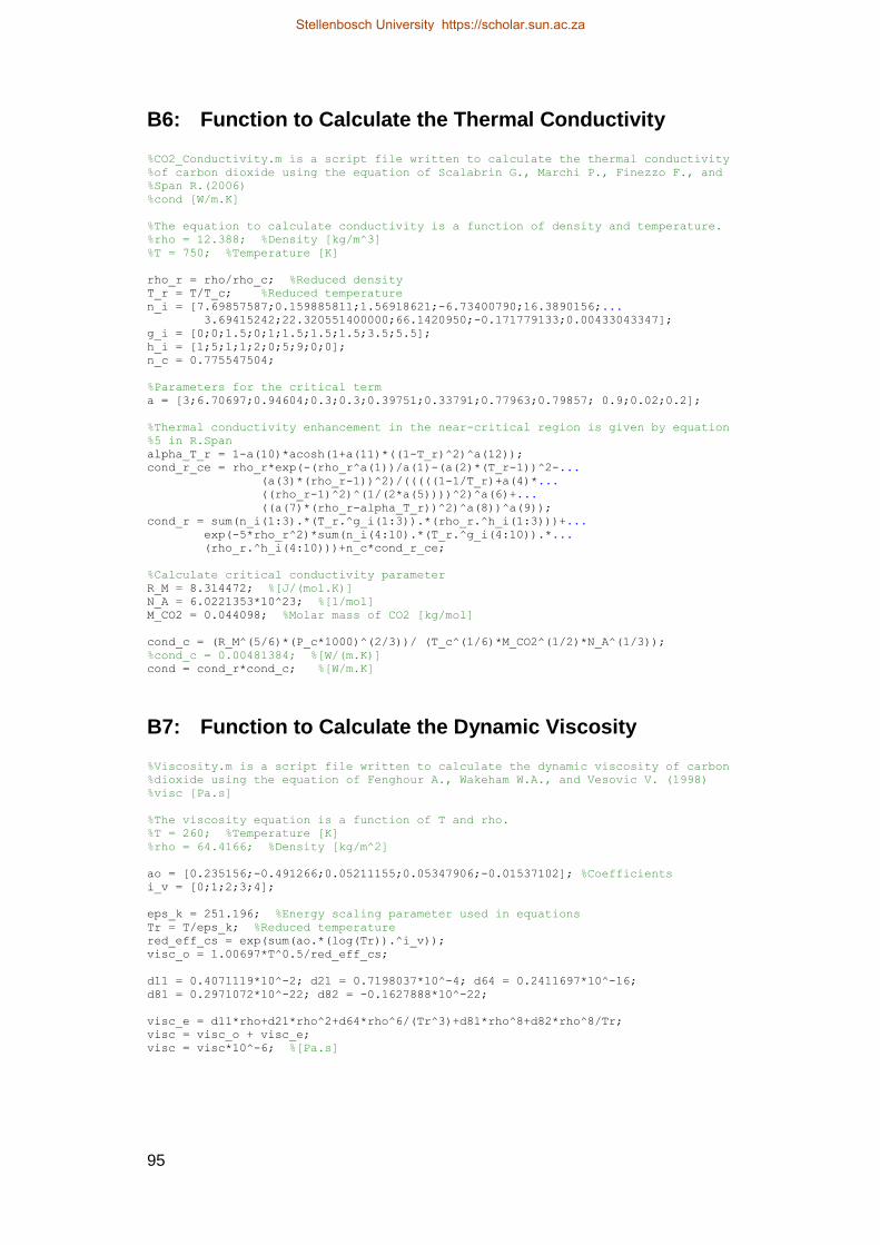
95

B6: Function to Calculate the Thermal Conductivity

%CO2_Conductivity.m is a script file written to calculate the thermal conductivity

%of carbon dioxide using the equation of Scalabrin G., Marchi P., Finezzo F., and

%Span R.(2006)

%cond [W/m.K]

%The equation to calculate conductivity is a function of density and temperature.

%rho = 12.388; %Density [kg/m^3]

%T = 750; %Temperature [K]

rho_r = rho/rho_c; %Reduced density

T_r = T/T_c; %Reduced temperature

n_i = [7.69857587;0.159885811;1.56918621;-6.73400790;16.3890156;...

3.69415242;22.320551400000;66.1420950;-0.171779133;0.00433043347];

g_i = [0;0;1.5;0;1;1.5;1.5;1.5;3.5;5.5];

h_i = [1;5;1;1;2;0;5;9;0;0];

n_c = 0.775547504;

%Parameters for the critical term

a = [3;6.70697;0.94604;0.3;0.3;0.39751;0.33791;0.77963;0.79857; 0.9;0.02;0.2];

%Thermal conductivity enhancement in the near-critical region is given by equation

%5 in R.Span

alpha_T_r = 1-a(10)*acosh(1+a(11)*((1-T_r)^2)â(12));

cond_r_ce = rho_r*exp(-(rho_râ(1))/a(1)-(a(2)*(T_r-1))^2-...

(a(3)*(rho_r-1))^2)/(((((1-1/T_r)+a(4)*...

((rho_r-1)^2)^(1/(2*a(5))))^2)â(6)+...

((a(7)*(rho_r-alpha_T_r))^2)â(8))â(9));

cond_r = sum(n_i(1:3).*(T_r.^g_i(1:3)).*(rho_r.^h_i(1:3)))+...

exp(-5*rho_r^2)*sum(n_i(4:10).*(T_r.^g_i(4:10)).*...

(rho_r.^h_i(4:10)))+n_c*cond_r_ce;

%Calculate critical conductivity parameter

R_M = 8.314472; %[J/(mol.K)]

N_A = 6.0221353*10^23; %[1/mol]

M_CO2 = 0.044098; %Molar mass of CO2 [kg/mol]

cond_c = (R_M^(5/6)*(P_c*1000)^(2/3))/ (T_c^(1/6)*M_CO2^(1/2)*N_A^(1/3));

%cond_c = 0.00481384; %[W/(m.K)]

cond = cond_r*cond_c; %[W/m.K]

B7: Function to Calculate the Dynamic Viscosity

%Viscosity.m is a script file written to calculate the dynamic viscosity of carbon

%dioxide using the equation of Fenghour A., Wakeham W.A., and Vesovic V. (1998)

%visc [Pa.s]

%The viscosity equation is a function of T and rho.

%T = 260; %Temperature [K]

%rho = 64.4166; %Density [kg/m^2]

ao = [0.235156;-0.491266;0.05211155;0.05347906;-0.01537102]; %Coefficients

i_v = [0;1;2;3;4];

eps_k = 251.196; %Energy scaling parameter used in equations

Tr = T/eps_k; %Reduced temperature

red_eff_cs = exp(sum(ao.*(log(Tr)).î_v));

visc_o = 1.00697*T^0.5/red_eff_cs;

d11 = 0.4071119*10^-2; d21 = 0.7198037*10^-4; d64 = 0.2411697*10^-16;

d81 = 0.2971072*10^-22; d82 = -0.1627888*10^-22;

visc_e = d11*rho+d21*rho^2+d64*rho^6/(Tr^3)+d81*rho^8+d82*rho^8/Tr;

visc = visc_o + visc_e;

visc = visc*10^-6; %[Pa.s]


96

B8: Function to Calculate the Properties at a Given Density and Specific Internal Energy

%CO2_Prop_at_rho_and_u.m is a script file written to calculate all properties of

%CO2 based on rho and u.

%Determine if the flow is single phase (1ph) or two phase (2ph) for a given

%density (rho) and internal energy (u), and then call the appropriate functions to

%calculate the thermodynamic properties as well as the thermal conductivity and

%dynamic viscosity

%rho = ; %Given density

%u = ; %Given specific internal energy

%rho_fi_2,rho_gi_2 and u_fi_2,u_gi_2 are vectors of saturated density and

%saturated %specific energy. These vectors are used to decide if the flow is two-

%phase or single %phase.

if (rho>=rho_fi_2(1))||(rho<=rho_gi_2(1))

CO2_1Ph_Prop_at_rho_and_u;

CO2_Conductivity; %Calculate conductivity given rho and T

Viscosity_CO2; %Calculate dynamic viscosity given rho and T

else

if rho>=rho_c

if rho<600

u_f_at_rho = interp1(rho_fi,u_fi,rho); %finer vector

else

u_f_at_rho = interp1(rho_fi_2,u_fi_2,rho); %coarser vector (for speed)

end

if abs(u-u_f_at_rho)<1 %Only recalculate if it is really close to the

%saturation line

CO2_Sat_Prop_at_rho_f

u_f_at_rho = u_f;

end

if u<(u_f_at_rho-1e-8) %Calculate two-phase properties


rho = rho_g; Viscosity_CO2; visc_g = visc;

CO2_Conductivity; cond_g = cond;

rho = rho_f; Viscosity_CO2; visc_f = visc;

CO2_Conductivity; cond_f = cond;

rho = rho_x; %Set density to its two-phase value

visc = 1/(xi/visc_g+(1-xi)/visc_f);

cond = 1/(xi/cond_g+(1-xi)/cond_f);

elseif abs(u-u_f_at_rho)<=1e-8

%Assign saturation properties

T=x(1); Two_ph = 0;

CO2_Property

CO2_Conductivity

Viscosity_CO2

else %Calculate single phase properties


CO2_Conductivity;

Viscosity_CO2;

end

elseif rho<rho_c

if rho>330

u_g_at_rho = interp1(rho_gi,u_gi,rho);

else

u_g_at_rho = interp1(rho_gi_2,u_gi_2,rho);

end

if abs(u-u_g_at_rho)<1 %Only recalculate if it is really close to the

%saturation line

CO2_Sat_Prop_at_rho_g

u_g_at_rho = u_g;

end

if u<(u_g_at_rho-1e-8) %Calculate two-phase properties



97





rho = rho_x; %Set density to its two phase value



elseif abs(u-u_g_at_rho)<=1e-8

%Assign saturation properties

T=x(1); Two_ph = 0;

CO2_Property

CO2_Conductivity

Viscosity_CO2

else %Calculate single phase properties


CO2_Conductivity;

Viscosity_CO2;

end

end

end

APPENDIX C: TRANSIENT SIMULATION PROGRAM

This section shows the program code for the transient simulation model of the

CO2 refrigeration cycle with capillary tube expansion device, as discussed in

section 4.

C1: Main Program Code of the Transient Simulation Model

%--------------------------------------------------------------------------------%

% Program code: Simulating_Refrigeration_cycle.m

% Transient simulation model of a sub- to trans-critical CO2 refrigeration system

% containing capillary tube as expansion device

% Author: Michael Garces de Gois

%--------------------------------------------------------------------------------%

Initialise_Refrigerator_System %Initialise the simulation domain

n_TS = 0; %Initialise time-step counter

while n_TS<700000

n_TS = n_TS+1;

Time_stepping_UD_density_based %Update variables to advance to the new time-

step

Itterate_UD_density_based %Iterate to solve variables of the new time-step

i_count %Display iteration count to reach convergence for the time-step

end


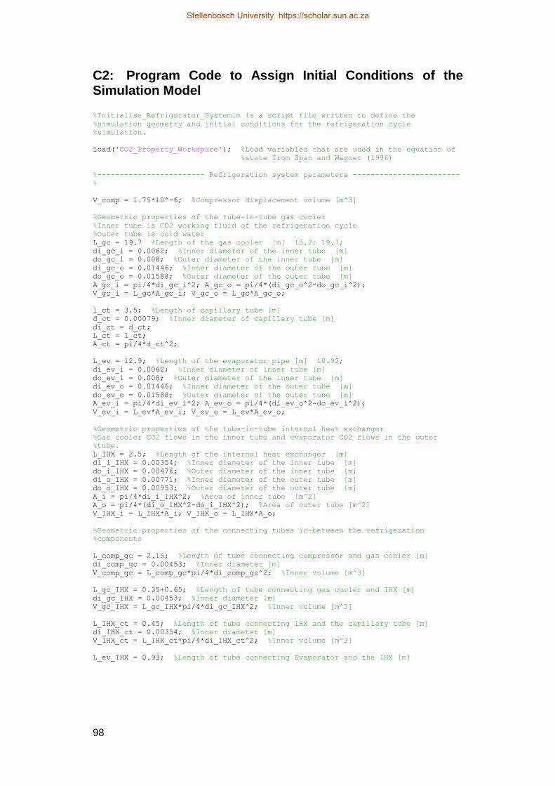
98

C2: Program Code to Assign Initial Conditions of the Simulation Model

%Initialise_Refrigerator_System.m is a script file written to define the

%simulation geometry and initial conditions for the refrigeration cycle

%simulation.

load('CO2_Property_Workspace'); %Load variables that are used in the equation of

%state from Span and Wagner (1996)

%------------------------ Refrigeration system parameters ------------------------

%

V_comp = 1.75*10^-6; %Compressor displacement volume [m^3]

%Geometric properties of the tube-in-tube gas cooler

%Inner tube is CO2 working fluid of the refrigeration cycle

%Outer tube is cold water

L_gc = 19.7 %Length of the gas cooler [m] 15.2; 19.7;

di_gc_i = 0.0062; %Inner diameter of the inner tube [m]

do_gc_i = 0.008; %Outer diameter of the inner tube [m]

di_gc_o = 0.01446; %Inner diameter of the outer tube [m]

do_gc_o = 0.01588; %Outer diameter of the outer tube [m]

A_gc_i = pi/4*di_gc_i^2; A_gc_o = pi/4*(di_gc_o^2-do_gc_i^2);

V_gc_i = L_gc*A_gc_i; V_gc_o = L_gc*A_gc_o;

l_ct = 3.5; %Length of capillary tube [m]

d_ct = 0.00079; %Inner diameter of capillary tube [m]

di_ct = d_ct;

L_ct = l_ct;

A_ct = pi/4*d_ct^2;

L_ev = 12.9; %Length of the evaporator pipe [m] 10.92;

di_ev_i = 0.0062; %Inner diameter of inner tube [m]

do_ev_i = 0.008; %Outer diameter of the inner tube [m]

di_ev_o = 0.01446; %Inner diameter of the outer tube [m]

do_ev_o = 0.01588; %Outer diameter of the outer tube [m]

A_ev_i = pi/4*di_ev_i^2; A_ev_o = pi/4*(di_ev_o^2-do_ev_i^2);

V_ev_i = L_ev*A_ev_i; V_ev_o = L_ev*A_ev_o;

%Geometric properties of the tube-in-tube internal heat exchanger

%Gas cooler CO2 flows in the inner tube and evaporator CO2 flows in the outer

%tube.

L_IHX = 2.5; %Length of the internal heat exchanger [m]

di_i_IHX = 0.00354; %Inner diameter of the inner tube [m]

do_i_IHX = 0.00476; %Outer diameter of the inner tube [m]

di_o_IHX = 0.00771; %Inner diameter of the outer tube [m]

do_o_IHX = 0.00953; %Outer diameter of the outer tube [m]

A_i = pi/4*di_i_IHX^2; %Area of inner tube [m^2]

A_o = pi/4*(di_o_IHX^2-do_i_IHX^2); %Area of outer tube [m^2]

V_IHX_i = L_IHX*A_i; V_IHX_o = L_IHX*A_o;

%Geometric properties of the connecting tubes in-between the refrigeration

%components

L_comp_gc = 2.15; %Length of tube connecting compressor and gas cooler [m]

di_comp_gc = 0.00453; %Inner diameter [m]

V_comp_gc = L_comp_gc*pi/4*di_comp_gc^2; %Inner volume [m^3]

L_gc_IHX = 0.35+0.65; %Length of tube connecting gas cooler and IHX [m]

di_gc_IHX = 0.00453; %Inner diameter [m]

V_gc_IHX = L_gc_IHX*pi/4*di_gc_IHX^2; %Inner volume [m^3]

L_IHX_ct = 0.45; %Length of tube connecting IHX and the capillary tube [m]

di_IHX_ct = 0.00354; %Inner diameter [m]

V_IHX_ct = L_IHX_ct*pi/4*di_IHX_ct^2; %Inner volume [m^3]

L_ev_IHX = 0.93; %Length of tube connecting Evaporator and the IHX [m]


99

di_ev_IHX = 0.00453; %Inner diameter [m]

V_ev_IHX = L_ev_IHX*pi/4*di_ev_IHX^2; %Inner volume [m^3]

L_IHX_comp = 0.35; %Length of tube connecting IHX to inlet of compressor [m]

di_IHX_comp = 0.00453; %Inner diameter [m]

V_IHX_comp = L_IHX_comp*pi/4*di_IHX_comp^2; %Inner volume [m^3]

%Lengths [m] of transition pieces between tubes of different diameters

L_tr1 = 0.015; %Between comp_gc and gc

L_tr2 = 0.015; %Between gc and gc_IHX

L_tr3 = 0.015; %Between gc_IHX and IHX inner tube (contains gas cooler CO2)

L_tr4 = 0.015; %Between IHX inner tube and IHX_ct

L_tr5 = 0.030; %Between IHX_ct and ct

L_tr6 = 0.030; %Between ct and ev

L_tr7 = 0.015; %Between ev and ev_IHX

L_tr8 = 0.045; %Between ev_IHX and IHX outer tube (Contains evaporator CO2)

L_tr9 = 0.045; %Between IHX outer tube and IHX_comp

%-------------------------------------------------------------------------%

%Form the control volumes of the whole solution domain.

N_comp_gc = 52; %Number of cv's for the connecting tube between outlet of

%compressor and inlet of gas cooler.

N_tr1 = 1; %Number of cv's for transition between comp_gc tube and gas

%cooler tube.

N_gc = 400; %Number of cv's for the gas cooler.

N_tr2 = 1; %Number of cv's for transition between gas cooler tube and

%gc_IHX tube

N_gc_IHX = 66; %Number of cv's between outlet of gas cooler and IHX.

N_tr3 = 1; %Number of cv's for transition between gc_IHX tube and

%IHX tube

N_IHX = 120; %Number of cv's for the Internal Heat Exchanger (IHX) inner tube.

N_tr4 = 1; %Number of cv's for transition between IHX tube and

%IHX_ct tube

N_IHX_ct = 24; %Number of cv's for the connecting tube between IHX and

%Capillary tube.

N_tr5 = 2; %Transition between IHX_ct tube and capillary tube

N_ct = 230; %Number of cv's for the Capillary Tube.

N_tr6 = 2; %Transition between capillary tube and evaporator tube

N_ev = 300; %Number of cv's for the Evaporator.

N_tr7 = 1; %Transition between evaporator tube and ev_IHX tube

N_ev_IHX = 40; %Number of cv's for the connecting tube between outlet of

%Evaporator and IHX.

N_tr8 = 3; %Transition between ev_IHX tube and IHX tube

%N_IHX = 120; %Number of cv's used for outer tube of IHX

N_tr9 = 3; %Transition between IHX tube and IHX_comp tube

N_IHX_comp = 23;%Number of cv's for the connecting tube between the IHX outlet

%and compressor inlet.

N_HP = N_comp_gc+N_tr1+N_gc+N_tr2+N_gc_IHX+N_tr3+N_IHX+N_tr4+N_IHX_ct+N_tr5;

N_LP = N_tr6+N_ev+N_tr7+N_ev_IHX+N_tr8+N_IHX+N_tr9+N_IHX_comp;

N_tot = N_HP+N_ct+N_LP;

%--Build a vector containing cv lengths--%

%Initialise control volume lengths

L_z(1:N_tot) = 0; %[m]

%Define lengths of control volumes for the different sections.

%comp_gc connecting pipe lengths

L_z(1:N_comp_gc/2) = Changing_Size_Mesh(L_comp_gc/2,1/0.9322,N_comp_gc/2);

L_z(N_comp_gc/2+1:N_comp_gc) = Changing_Size_Mesh(L_comp_gc/2,0.9322,N_comp_gc/2);

%tr1 cv lengths

L_z(N_comp_gc+1:N_comp_gc+N_tr1) = L_tr1/N_tr1;

%Gas cooler cv lengths

L_z(N_comp_gc+N_tr1+1:N_comp_gc+N_tr1+N_gc/2) =

Changing_Size_Mesh(L_gc/2,1/0.98981,N_gc/2);

L_z(N_comp_gc+N_tr1+N_gc/2+1:N_comp_gc+N_tr1+N_gc) =

Changing_Size_Mesh(L_gc/2,0.98981,N_gc/2);

%tr2 cv lengths

L_z(N_comp_gc+N_tr1+N_gc+1:N_comp_gc+N_tr1+N_gc+N_tr2) = L_tr2/N_tr2;


100

%gc_IHX cv lengths

L_z(N_comp_gc+N_tr1+N_gc+N_tr2+1:N_comp_gc+N_tr1+N_gc+N_tr2+N_gc_IHX) =

L_gc_IHX/N_gc_IHX;

%tr3 cv lengths

L_z(N_comp_gc+N_tr1+N_gc+N_tr2+N_gc_IHX+1:N_comp_gc+N_tr1+N_gc+N_tr2+N_gc_IHX+N_tr

3)= L_tr3/N_tr3;

%IHX cv lengths

%Gas cooler side of IHX's cv lengths

L_z(N_HP-(N_IHX+N_tr4+N_IHX_ct+N_tr5)+1:N_HP-(N_IHX/2+N_tr4+N_IHX_ct+N_tr5)) =

Changing_Size_Mesh(L_IHX/2,1/0.9895,N_IHX/2);

L_z(N_HP-(N_IHX/2+N_tr4+N_IHX_ct+N_tr5)+1:N_HP-(N_tr4+N_IHX_ct+N_tr5)) =

Changing_Size_Mesh(L_IHX/2,0.9895,N_IHX/2);

%tr4 cv lengths

L_z(N_HP-(N_tr4+N_IHX_ct+N_tr5)+1:N_HP-(N_IHX_ct+N_tr5)) = L_tr4/N_tr4;

%IHX_ct cv lengths

L_z(N_HP-(N_IHX_ct+N_tr5)+1:N_HP-(N_IHX_ct/2+N_tr5)) =

Changing_Size_Mesh(L_IHX_ct/2,1/0.9619,N_IHX_ct/2);

L_z(N_HP-(N_IHX_ct/2+N_tr5)+1:N_HP-(N_tr5)) =

Changing_Size_Mesh(L_IHX_ct/2,0.9619,N_IHX_ct/2);

%tr5 cv lengths (Transition to capillary tube)

L_z(N_HP-(N_tr5)+1:N_HP) = L_tr5/N_tr5;

%ct (capillary tube) cv lengths

L_z(N_HP+1:N_HP+N_ct) = L_ct/N_ct;

%tr6 cv lengths (Transition from capillary tube to evaporator tube)

L_z(N_HP+N_ct+1:N_HP+N_ct+N_tr6) = L_tr6/N_tr6;

%Evaporator cv lengths

L_z(N_HP+N_ct+N_tr6+1:N_HP+N_ct+N_tr6+N_ev/2) =

Changing_Size_Mesh(L_ev/2,1/0.98779,N_ev/2);

L_z(N_HP+N_ct+N_tr6+N_ev/2+1:N_HP+N_ct+N_tr6+N_ev) =

Changing_Size_Mesh(L_ev/2,0.98779,N_ev/2);

%tr7 cv lengths

L_z(N_HP+N_ct+N_tr6+N_ev+1:N_HP+N_ct+N_tr6+N_ev+N_tr7) = L_tr7/N_tr7;

%ev_IHX cv lengths

L_z(N_HP+N_ct+N_tr6+N_ev+N_tr7+1:N_HP+N_ct+N_tr6+N_ev+N_tr7+N_ev_IHX/2) =

Changing_Size_Mesh(L_ev_IHX/2,1/0.958,N_ev_IHX/2);

L_z(N_HP+N_ct+N_tr6+N_ev+N_tr7+N_ev_IHX/2+1:N_HP+N_ct+N_tr6+N_ev+N_tr7+N_ev_IHX) =

Changing_Size_Mesh(L_ev_IHX/2,0.958,N_ev_IHX/2);

%tr8 cv lengths

L_z(N_HP+N_ct+N_tr6+N_ev+N_tr7+N_ev_IHX+1:N_HP+N_ct+N_tr6+N_ev+N_tr7+N_ev_IHX+N_tr

8) = L_tr8/N_tr8;

%IHX cv lengths

%Evaporator side of IHX's cv lengths

%k is outer tube

for k=(N_tot-(N_tr9+N_IHX_comp)):-1:((N_tot-(N_IHX+N_tr9+N_IHX_comp)+1))

%k_i is cv number of inner tube cv exchanging heat with the outer k'th cv

k_i = ((N_tot-(N_tr9+N_IHX_comp))-k+1)+

(N_comp_gc+N_tr1+N_gc+N_tr2+N_gc_IHX+N_tr3);

L_z(k) = L_z(k_i);

end

%tr9 cv lengths

L_z(N_tot-(N_tr9+N_IHX_comp)+1:N_tot-(N_IHX_comp)) = L_tr9/N_tr9;

%IHX_comp cv lengths

L_z(N_tot-(N_IHX_comp)+1:N_tot) = L_IHX_comp/N_IHX_comp;

%Define area and hydraulic diameter of control volumes

A_v(1:N_tot+1) = 0; %[m^2]

dh(1:N_tot) = 0; %[m]

%comp_gc

A_v(1) = pi/4*di_comp_gc^2; %Inlet area of 1st cv

for k=1:N_comp_gc

A_v(k+1) = pi/4*di_comp_gc^2; %Cross sectional area at outlet of cv [m^2]

dh(k) = di_comp_gc;

end

%tr1

for k=(N_comp_gc+1):(N_comp_gc+N_tr1)

A_v(k+1) = (pi/4*(di_gc_i^2-

di_comp_gc^2)/L_tr1)*sum(L_z(N_comp_gc+1:k))+pi/4*di_comp_gc^2;

dh(k) = sqrt(((A_v(k)+A_v(k+1))/2)*4/pi);

end


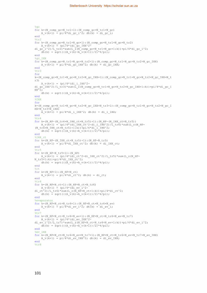
101

%gc

for k=(N_comp_gc+N_tr1+1):(N_comp_gc+N_tr1+N_gc)

A_v(k+1) = pi/4*di_gc_i^2; dh(k) = di_gc_i;

end

%tr2

for k=(N_comp_gc+N_tr1+N_gc+1):(N_comp_gc+N_tr1+N_gc+N_tr2)

A_v(k+1) = (pi/4*(di_gc_IHX^2-

di_gc_i^2)/L_tr2)*sum(L_z(N_comp_gc+N_tr1+N_gc+1:k))+pi/4*di_gc_i^2;


end

%gc_IHX

for k=(N_comp_gc+N_tr1+N_gc+N_tr2+1):(N_comp_gc+N_tr1+N_gc+N_tr2+N_gc_IHX)

A_v(k+1) = pi/4*di_gc_IHX^2; dh(k) = di_gc_IHX;

end

%tr3

for

k=(N_comp_gc+N_tr1+N_gc+N_tr2+N_gc_IHX+1):(N_comp_gc+N_tr1+N_gc+N_tr2+N_gc_IHX+N_t

r3)

A_v(k+1) = (pi/4*(di_i_IHX^2-

di_gc_IHX^2)/L_tr3)*sum(L_z(N_comp_gc+N_tr1+N_gc+N_tr2+N_gc_IHX+1:k))+pi/4*di_gc_I

HX^2;


end

%IHX

for

k=(N_comp_gc+N_tr1+N_gc+N_tr2+N_gc_IHX+N_tr3+1):(N_comp_gc+N_tr1+N_gc+N_tr2+N_gc_I

HX+N_tr3+N_IHX)

A_v(k+1) = pi/4*di_i_IHX^2; dh(k) = di_i_IHX;

end

%tr4

for k=(N_HP-(N_tr4+N_IHX_ct+N_tr5)+1):(N_HP-(N_IHX_ct+N_tr5))

A_v(k+1) = (pi/4*(di_IHX_ct^2-di_i_IHX^2)/L_tr4)*sum(L_z(N_HP-

(N_tr4+N_IHX_ct+N_tr5)+1:k))+pi/4*di_i_IHX^2;


end

%IHX_ct

for k=(N_HP-(N_IHX_ct+N_tr5)+1):(N_HP-N_tr5)

A_v(k+1) = pi/4*di_IHX_ct^2; dh(k) = di_IHX_ct;

end

%tr5

for k=(N_HP-N_tr5+1):(N_HP)

A_v(k+1) = (pi/4*(di_ct^2-di_IHX_ct^2)/L_tr5)*sum(L_z(N_HP-

N_tr5+1:k))+pi/4*di_IHX_ct^2;


end

%ct

for k=(N_HP+1):(N_HP+N_ct)

A_v(k+1) = pi/4*di_ct^2; dh(k) = di_ct;

end

%tr6

for k=(N_HP+N_ct+1):(N_HP+N_ct+N_tr6)

A_v(k+1) = (pi/4*(di_ev_i^2-

di_ct^2)/L_tr6)*sum(L_z(N_HP+N_ct+1:k))+pi/4*di_ct^2;


end

%evaporator

for k=(N_HP+N_ct+N_tr6+1):(N_HP+N_ct+N_tr6+N_ev)

A_v(k+1) = pi/4*di_ev_i^2; dh(k) = di_ev_i;

end

%tr7

for k=(N_HP+N_ct+N_tr6+N_ev+1):(N_HP+N_ct+N_tr6+N_ev+N_tr7)

A_v(k+1) = (pi/4*(di_ev_IHX^2-

di_ev_i^2)/L_tr7)*sum(L_z(N_HP+N_ct+N_tr6+N_ev+1:k))+pi/4*di_ev_i^2;


end

%ev_IHX

for k=(N_HP+N_ct+N_tr6+N_ev+N_tr7+1):(N_HP+N_ct+N_tr6+N_ev+N_tr7+N_ev_IHX)

A_v(k+1) = pi/4*di_ev_IHX^2; dh(k) = di_ev_IHX;

end

%tr8


102

for

k=(N_HP+N_ct+N_tr6+N_ev+N_tr7+N_ev_IHX+1):(N_HP+N_ct+N_tr6+N_ev+N_tr7+N_ev_IHX+N_t

r8)

A_v(k+1) = (pi/4*((di_o_IHX^2-do_i_IHX^2)-

di_ev_IHX^2)/L_tr8)*sum(L_z(N_HP+N_ct+N_tr6+N_ev+N_tr7+N_ev_IHX+1:k))+pi/4*di_ev_I

HX^2;


end

%IHX outer tube

for

k=(N_HP+N_ct+N_tr6+N_ev+N_tr7+N_ev_IHX+N_tr8+1):(N_HP+N_ct+N_tr6+N_ev+N_tr7+N_ev_I

HX+N_tr8+N_IHX)

A_v(k+1) = pi/4*(di_o_IHX^2-do_i_IHX^2); dh(k) = (di_o_IHX-do_i_IHX);

end

%tr9

for k=(N_tot-(N_tr9+N_IHX_comp)+1):(N_tot-(N_IHX_comp))

A_v(k+1) = (pi/4*(di_IHX_comp^2-(di_o_IHX^2-do_i_IHX^2))/L_tr9)*sum(L_z(N_tot-

(N_tr9+N_IHX_comp)+1:k))+pi/4*(di_o_IHX^2-do_i_IHX^2);


end

%IHX_comp

for k=(N_tot-N_IHX_comp+1):N_tot

A_v(k+1) = pi/4*di_IHX_comp^2; dh(k) = di_IHX_comp;

end

%----------------------------- Initial state -----------------------------%

%Calculate total volume of the refrigerator system

Vol_HP = 0; %Calculate the volume of the high pressure side

for k=1:N_HP

Vol_HP = Vol_HP+(A_v(k)+A_v(k+1))/2*L_z(k);

end

Vol_ct = 0; %Calculate the volume of the capillary tube

for k=(N_HP+1):(N_HP+N_ct)

Vol_ct = Vol_ct+(A_v(k)+A_v(k+1))/2*L_z(k);

end

Vol_LP = 0; %Calculate the volume of the low pressure side

for k=(N_HP+N_ct+1):(N_tot)

Vol_LP = Vol_LP+(A_v(k)+A_v(k+1))/2*L_z(k);

end

Vol_Total = Vol_HP+Vol_ct+Vol_LP;

m_Total_CO2 = 0.435; %Total mass of CO2 in system [kg]

rho_initial = m_Total_CO2/Vol_Total; %Initial average density in the system

T_initial = 25+273.15; %Assume the system is in equilibrium with its environment

%Determine the state of the CO2 working fluid at the start

rho = rho_initial;

T = T_initial;

CO2_Prop_at_rho_and_T; %Determines all properties of CO2 at the given initial

state

P_initial = P; %Pressure at the start (kPa)

%Define and initialise vectors to hold the vapour quality and other values of CO2

rho_f_z(1:N_tot)=1000; %Initialise

rho_g_z(1:N_tot)=10; %Initialise

alpha_vol_z(1:N_tot)=0.9; %Initialise

xi_z(1:N_tot)=1; %Initialise

%If two phase is present in the initial state

if Two_ph==1

m_f = (1-xi)*m_Total_CO2;

Vol_f = m_f/rho_f;

if Vol_HP<=Vol_f

for k=1:N_tot

%Assume for the simulation that at all liquid is contained in the first

%control volumes of the HP side at start-up. (This is a fair assumption

%since the refrigerator is charged in the HP side and also most CO2 settles

%in the HP side at the end of operation).

m_z(k) = rho_f*(A_v(k)+A_v(k+1))/2*L_z(k); rho_z(k) = rho_f;

u_z(k) = u_f; z(k) = cp_f; cv_z(k) = cv_f; h_z(k) = h_f; s_z(k) = s_f;


103

cond_z(k) = cond_f; mu_z(k) = visc_f;

rho_f_z(k) = rho_f; rho_g_z(k) = rho_g;

alpha_vol_z(k) = 0; xi_z(k) = 0;

if sum(m_z(1:k))>m_f

%Correct the properties of the current control volume (transition cv)

m_f_k = m_f-sum(m_z(1:k-1));

vol_f_k = m_f_k/rho_f;

vol_g_k = ((A_v(k)+A_v(k+1))/2*L_z(k))-vol_f_k;

m_g_k = vol_g_k*rho_g;

xi = m_g_k/(m_g_k+m_f_k); %vapour fraction

m_z(k) = m_f_k+m_g_k; rho_z(k) = m_z(k)/((A_v(k)+A_v(k+1))/2*L_z(k));

u_z(k) = xi*u_g+(1-xi)*u_f; h_z(k) = xi*h_g+(1-xi)*h_f;

s_z(k) = xi*s_g+(1-xi)*s_f; cp_z(k) = xi*cp_g+(1-xi)*cp_f;

cv_z(k) = xi*cv_g+(1-xi)*cv_f; cond_z(k) = (xi/cond_g+(1-xi)/cond_f)^-

1;

mu_z(k) = (xi/visc_g+(1-xi)/visc_f)^-1; rho_f_z(k) = rho_f;

rho_g_z(k) = rho_g; alpha_vol_z(k) = vol_g_k/(vol_g_k+vol_f_k);

xi_z(k) = xi;

k_trans = k;

break %Leave the for loop

end

end

%Remainder of refrigeration system will contain saturated gas only

for k=(k_trans+1):N_tot

m_z(k) = rho_g*(A_v(k)+A_v(k+1))/2*L_z(k); rho_z(k) = rho_g;

u_z(k) = u_g; cp_z(k) = cp_g; cv_z(k) = cv_g; h_z(k) = h_g;

s_z(k) = s_g; cond_z(k) = cond_g; mu_z(k) = visc_g;

rho_f_z(k) = rho_f;

rho_g_z(k) = rho_g; alpha_vol_z(k) = 1; xi_z(k) = 1;

end

else

for k=N_HP:-1:1

m_z(k) = rho_f*(A_v(k)+A_v(k+1))/2*L_z(k); rho_z(k) = rho_f;

u_z(k) = u_f; cp_z(k) = cp_f; cv_z(k) = cv_f; h_z(k) = h_f;

s_z(k) = s_f;

cond_z(k) = cond_f; mu_z(k) = visc_f; rho_f_z(k) = rho_f;


if sum(m_z(N_HP:-1:k))>m_f

%Correct the current properties for the transition control volume

m_f_k = m_f-sum(m_z(N_HP:-1:k+1));

vol_f_k = m_f_k/rho_f;

vol_g_k = ((A_v(k)+A_v(k+1))/2*L_z(k))-vol_f_k;

m_g_k = vol_g_k*rho_g;

xi = m_g_k/(m_g_k+m_f_k); %vapour fraction

m_z(k) = m_f_k+m_g_k; rho_z(k) =

m_z(k)/((A_v(k)+A_v(k+1))/2*L_z(k));

u_z(k) = xi*u_g+(1-xi)*u_f; h_z(k) = xi*h_g+(1-xi)*h_f;

s_z(k) = xi*s_g+(1-xi)*s_f; cp_z(k) = xi*cp_g+(1-xi)*cp_f;

cv_z(k) = xi*cv_g+(1-xi)*cv_f; cond_z(k) = (xi/cond_g+(1-

xi)/cond_f)^-1;

mu_z(k) = (xi/visc_g+(1-xi)/visc_f)^-1; rho_f_z(k) = rho_f;

rho_g_z(k) = rho_g; alpha_vol_z(k) = vol_g_k/(vol_g_k+vol_f_k);

xi_z(k) = xi;

k_trans = k;

break %Leave the for loop

end

end

%Remainder of HP side will contain saturated gas only

for k=(k_trans-1):-1:1


u_z(k) = u_g;

cp_z(k) = cp_g; cv_z(k) = cv_g; h_z(k) = h_g; s_z(k) = s_g;


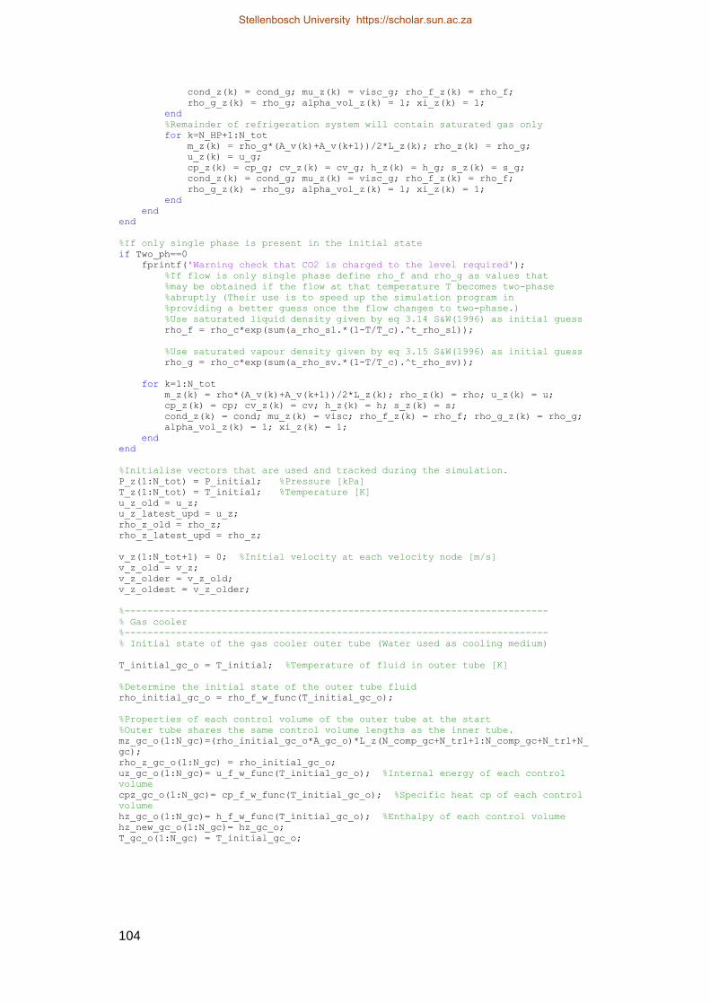
104

cond_z(k) = cond_g; mu_z(k) = visc_g; rho_f_z(k) = rho_f;


end

%Remainder of refrigeration system will contain saturated gas only

for k=N_HP+1:N_tot


u_z(k) = u_g;

cp_z(k) = cp_g; cv_z(k) = cv_g; h_z(k) = h_g; s_z(k) = s_g;

cond_z(k) = cond_g; mu_z(k) = visc_g; rho_f_z(k) = rho_f;


end

end

end

%If only single phase is present in the initial state

if Two_ph==0

fprintf('Warning check that CO2 is charged to the level required');

%If flow is only single phase define rho_f and rho_g as values that

%may be obtained if the flow at that temperature T becomes two-phase

%abruptly (Their use is to speed up the simulation program in

%providing a better guess once the flow changes to two-phase.)

%Use saturated liquid density given by eq 3.14 S&W(1996) as initial guess


%Use saturated vapour density given by eq 3.15 S&W(1996) as initial guess


for k=1:N_tot

m_z(k) = rho*(A_v(k)+A_v(k+1))/2*L_z(k); rho_z(k) = rho; u_z(k) = u;

cp_z(k) = cp; cv_z(k) = cv; h_z(k) = h; s_z(k) = s;

cond_z(k) = cond; mu_z(k) = visc; rho_f_z(k) = rho_f; rho_g_z(k) = rho_g;


end

end

%Initialise vectors that are used and tracked during the simulation.

P_z(1:N_tot) = P_initial; %Pressure [kPa]

T_z(1:N_tot) = T_initial; %Temperature [K]

u_z_old = u_z;

u_z_latest_upd = u_z;

rho_z_old = rho_z;

rho_z_latest_upd = rho_z;

v_z(1:N_tot+1) = 0; %Initial velocity at each velocity node [m/s]

v_z_old = v_z;

v_z_older = v_z_old;

v_z_oldest = v_z_older;

%--------------------------------------------------------------------------

% Gas cooler

%--------------------------------------------------------------------------

% Initial state of the gas cooler outer tube (Water used as cooling medium)

T_initial_gc_o = T_initial; %Temperature of fluid in outer tube [K]

%Determine the initial state of the outer tube fluid

rho_initial_gc_o = rho_f_w_func(T_initial_gc_o);

%Properties of each control volume of the outer tube at the start

%Outer tube shares the same control volume lengths as the inner tube.

mz_gc_o(1:N_gc)=(rho_initial_gc_o*A_gc_o)*L_z(N_comp_gc+N_tr1+1:N_comp_gc+N_tr1+N_

gc);

rho_z_gc_o(1:N_gc) = rho_initial_gc_o;

uz_gc_o(1:N_gc)= u_f_w_func(T_initial_gc_o); %Internal energy of each control

volume

cpz_gc_o(1:N_gc)= cp_f_w_func(T_initial_gc_o); %Specific heat cp of each control

volume

hz_gc_o(1:N_gc)= h_f_w_func(T_initial_gc_o); %Enthalpy of each control volume

hz_new_gc_o(1:N_gc)= hz_gc_o;

T_gc_o(1:N_gc) = T_initial_gc_o;


105

cond_gc_o(1:N_gc) = cond_f_w_func(T_initial_gc_o);

mu_gc_o(1:N_gc) = mu_f_w_func(T_initial_gc_o);

uz_gc_o_latest_upd = uz_gc_o;

%Fixed operating conditions for the gas cooler outer tube (Cooling water)

mdot_gc_o = 0.045; %Mass flow rate through outer tube [kg/s]

%Temperature of entering fluid in outer tube

T_in_gc_o = 25 + 273.15; %Water at 25 deg C enters the outer tube of gas cooler

h_in_gc_o = h_f_w_func(T_in_gc_o); %Enthalpy of incoming flow for the outer tube

%[kJ/kg]

u_in_gc_o = u_f_w_func(T_in_gc_o); %Internal energy of incoming flow for the

outer %tube [kJ/kg]

%--------------------------------------------------------------------------

% Evaporator

%--------------------------------------------------------------------------

% Initial state of the evaporator outer tube

T_initial_ev_o = T_initial; %Temperature of fluid in outer tube [K]

%Determine the initial state of the outer tube fluid

rho_initial_ev_o = rho_f_w_func(T_initial_ev_o);

%Mass in each control volume of the outer tube at the start

mz_ev_o(1:N_ev)=(rho_initial_ev_o*A_ev_o)*L_z(N_HP+N_ct+N_tr6+1:N_HP+N_ct+N_tr6+N_

ev);

rho_z_ev_o(1:N_ev) = rho_initial_ev_o;

uz_ev_o(1:N_ev)= u_f_w_func(T_initial_ev_o); %Internal energy of each control

volume

cpz_ev_o(1:N_ev)= cp_f_w_func(T_initial_ev_o); %Specific heat cp of each control

volume

hz_ev_o(1:N_ev)= h_f_w_func(T_initial_ev_o); %Enthalpy of each control volume

hz_new_ev_o(1:N_ev)= hz_ev_o;

T_ev_o(1:N_ev) = T_initial_ev_o;

cond_ev_o(1:N_ev) = cond_f_w_func(T_initial_ev_o);

mu_ev_o(1:N_ev) = mu_f_w_func(T_initial_ev_o);

uz_ev_o_latest_upd = uz_ev_o;

%Fixed operating conditions for the evaporator outer tube (Heating water)

mdot_ev_o = 0.045; %Mass flow rate through outer tube [kg/s]

%Temperature of entering fluid in outer tube

T_in_ev_o = 25 + 273.15; %Water at 25 deg C enters the outer tube of evaporator

h_in_ev_o = h_f_w_func(T_in_ev_o); %Enthalpy of incoming flow for the outer tube

[kJ/kg]

u_in_ev_o = u_f_w_func(T_in_ev_o); %Internal energy of incoming flow for the

outer tube [kJ/kg]

%--------------------------------------------------------------------------

alpha_vol = 0.1; %Initial guess to determine two-phase properties

%------------------ Simulation of the refrigeration cycle ----------------%

dt = 1e-4; %Time step size [s]

t = 0; %Initialise time

rho_out_comp = rho_g/2; %Define an initial guess for the outlet density of the

%compressor

%Define vector to store location of cell centered nodes

L(1:N_tot)=0;

L(1) = L_z(1)/2;

for k=2:N_tot

L(k) = L(k-1)+L_z(k-1)/2+L_z(k)/2;

end

%Initialise variables used in the discretisation of conservation equations

%Variables for scalar control volumes

F_w = 0; F_e = 0;

a_w(1:N_tot) = 0; a_e(1:N_tot) = 0; a_p(1:N_tot) = 0; a_p_old (1:N_tot) = 0;

S_u(1:N_tot) = 0; S_p = 0; Qdot_ht(1:N_tot) = 0;

%Variables for momentum control volumes (on the staggered grid)


106

F_w_mom = 0;F_e_mom = 0;

a_w_mom(1:N_tot+1) = 0; a_e_mom(1:N_tot+1) = 0; a_p_mom(1:N_tot+1) = 0;

S_u_mom(1:N_tot+1) = 0; S_p_mom(1:N_tot+1) = 0; a_p_old_mom(1:N_tot+1) = 0;

rho_e(1:N_tot-1) = 0; %Initialise for later use

rho_z_new = rho_z;

u_z_new = u_z;

v_z_new = v_z;

C3: Program Code to Update Variables for the New Time-Step

%Time_stepping_UD_density_based.m is a script file written to update the old

values, %hence to advance the simulation to the new time-step.

%Update to new time level

v_z_oldest_old = v_z_oldest; v_z_oldest = v_z_older; v_z_older = v_z_old;

v_z_old = v_z;

%Use Taylor series expansion combined with backward-finite difference formulas for

the %derivatives to provide a projection method for determining a good guess for

the new %velocity field.

%Third order projection method gives:

v_z = 8/3*v_z_old-2.5*v_z_older+v_z_oldest-1/6*v_z_oldest_old; %Gives fastest

performance

rho_z_old = rho_z; u_z_old = u_z; T_z_old = T_z;

%Gas cooler water (outer tube)

uz_gc_o_old = uz_gc_o;

%Evaporator water (outer tube)

uz_ev_o_old = uz_ev_o;

C4: Program Code to Solve the Three Conservation Equations

%Itterate_UD_density_based.m is a script file written to iteratively solve the

%three conservation equations for a time-step using a density based algorithm.

%-------------------------

sum_u_mom_residuals=1; norm_Global_mom_Residual=1;

i_count = 0;

while (norm_Global_mom_Residual>10^-6)||(norm_Global_c_Residual>10^-6)...

||(norm_Global_e_Residual>10^-6)

i_count = i_count+1; % Count number of iterations per time-step

% Calculate boundary conditions

%-------------------- Compressor modelling (State 1-2) -------------------%

%Input variables

rho_in_comp = rho_z(N_tot); %Exit of last control volume is entrance to the

compressor

h1 = h_z(N_tot); s1 = s_z(N_tot); rho1 = rho_in_comp;

eff_volumetric = 0.954; eff_isentropic = 0.716;

V_comp = 1.75*10^-6; %Compressor displacement volume [m^3]

N = 2400; %Compressor speed [rev/min]

s2_isen = s1;

P2 = P_z(1); %Outlet pressure of the compressor [kPa]

s = s2_isen; P = P2;

T = T_z(1); %Use old value as initial guess


107

rho = rho_out_comp; %Use old value as initial guess (Note this is only a guess)

CO2_1Ph_Prop_at_P_and_s;

h2_isen = h;

h_comp_out = h1+(h2_isen-h1)/eff_isentropic;

h = h_comp_out; P = P2;

T = T_z(1); %Use old value as initial guess

rho = rho_out_comp; %Use old value as initial guess

CO2_1Ph_Prop_at_P_and_h;

%Obtained boundary conditions for the inlet of the simulation domain.

rho_out_comp = rho;

u_out_comp = u;

%Compressor mass flow rate boundary condition for the simulation domain.

mdot_comp = rho1*V_comp*N/60*eff_volumetric;

v_in = mdot_comp/(rho_out_comp*A_v(1));

v_out = mdot_comp/(rho_z(N_tot)*A_v(N_tot+1));

%Incorporate velocity boundary conditions for the simulation domain

v_z(1) = v_in; %Inlet boundary velocity of first control volume

v_z(N_tot+1) = v_out; %Outlet velocity of last control volume

%-------------------------------------------------------------------------%

%--Continuity equation--%

%First control volume

k=1;

L_PE = L_z(k)/2+L_z(k+1)/2; fe = (L_z(k+1)/2)/L_PE;

F_w = 0; F_e = v_z(k+1)*A_v(k+1);

a_w(k) = 0; a_e(k) = max(0,-F_e); a_p_old(k) = (A_v(k)+A_v(k+1))/2*L_z(k)/dt;

S_u(k) = mdot_comp+a_p_old(k)*rho_z_old(k);

a_p(k) = a_w(k)+a_e(k)+(F_e-F_w)+a_p_old(k);

for k=2:N_tot-1 %Interior control volumes


L_WP = L_z(k-1)/2+L_z(k)/2; fw = (L_z(k-1)/2)/L_WP;

F_w = v_z(k)*A_v(k); F_e = v_z(k+1)*A_v(k+1);

a_w(k) = max(F_w,0); a_e(k) = max(0,-F_e);

a_p_old(k) = (A_v(k)+A_v(k+1))/2*L_z(k)/dt;

S_u(k) = a_p_old(k)*rho_z_old(k);

a_p(k) = a_w(k)+a_e(k)+F_e-F_w+a_p_old(k);

end

%Last control volume

k=N_tot;


F_w = v_z(k)*A_v(k); F_e = 0;

a_w(k) = max(F_w,0); a_e(k) = 0; a_p_old(k) = (A_v(k)+A_v(k+1))/2*L_z(k)/dt;

S_u(k) = -mdot_comp+a_p_old(k)*rho_z_old(k);

a_p(k) = a_w(k)+a_e(k)+F_e-F_w+a_p_old(k);

%-------------------------------------------------------------------------%

%Check how well the current density satisfies the continuity equation:

%Calculate density(continuity) residuals at each cv

c_residual(1:N_tot) = 0;

%For first control volume

k=1;

c_residual(k) = a_p(k)*rho_z(k)-(a_e(k)*rho_z(k+1)+S_u(k));

c_norm_factor(k) = a_p(k)*rho_z(k);

for k=2:(N_tot-1) %Interior control volumes

c_residual(k) = a_p(k)*rho_z(k)-(a_w(k)*rho_z(k-1)+a_e(k)*rho_z(k+1)+S_u(k));


end

%For the last control volume

k=N_tot;

c_residual(k) = a_p(k)*rho_z(k)-(a_w(k)*rho_z(k-1)+S_u(k));


%Calculate sum of absolute momentum residuals

sum_c_residuals = sum(abs(c_residual(:)));


108

sum_c_norm_factor = sum(abs(c_norm_factor(:)));

%This gives an indication of how well the continuity equation is satisfied

norm_Global_c_Residual = sum_c_residuals/sum_c_norm_factor;

%-------------------------------------------------------------------------%

%TDMA solver for continuity equation (calculate new densities)

%-------------------------------------------------------------------------%

%alpha = a_e_c(k); %beta = a_w_c(k); %Dj = a_p_c(k);

%Boundary control volume

k=1;

Aj(k) = a_e(k)/(a_p(k)-0);

Cj_aks(k) = (0+S_u(k))/(a_p(k)-0);


Aj(k) = a_e(k)/(a_p(k)-a_w(k)*Aj(k-1));

Cj_aks(k) = (a_w(k)*Cj_aks(k-1)+S_u(k))/(a_p(k)-a_w(k)*Aj(k-1));

end

k=N_tot; %Last control volume

Aj(k) = 0;


for k=N_tot:-1:1

if k==N_tot, rho_z(k) = Cj_aks(k);

else rho_z(k) = Aj(k)*rho_z(k+1)+Cj_aks(k);

end

end

%Obtain face values for density

for k=1:N_tot-1

%Upwind differencing used for density

if v_z(k+1)>0, rho_e(k) = rho_z(k);

else rho_e(k) = rho_z(k+1);

end

end

%-------------------------------------------------------------------------%

%--Energy equation--%

%Calculate heat transfer (Radial heat transfer)

%Innitialise heat transfer and afterwards change the required cv's that do

%have heat transfer.

Qdot_ht(1:N_tot) = 0;

%--Gas cooler heat transfer rate--%

%Heat transfer rate for control volumes transferring heat between the

%gas cooler outer tube (water) and inner tube (CO2);

%Heat transfer rate defined positive as heat from the outer tube to the

%inner tube i.e. as heat addition to the CO2.

for k=(N_comp_gc+N_tr1+1):(N_comp_gc+N_tr1+N_gc)

%control volume nr for outer tube

k_o = k-(N_comp_gc+N_tr1);

if k>299 %Only 14 m of water cooling used, the rest has no heat transfer

Qdot_ht(k) = 0;

else %Heat exhange with water in the outer tube

Re_flow = rho_z(k)*abs((v_z(k)+v_z(k+1))/2)*di_gc_i/mu_z(k);

k_Cu = 400; %Thermal conductivity of copper [W/m.K]

%Thermal resistance for conduction through copper inner tube

R_i_Cu = log(do_gc_i/di_gc_i)/(2*pi*k_Cu*L_z(k)); %[K/W]

%Calculate inner tube heat transfer coefficient (ht_i)

%mu_z(k); %[Pa.s]

%cp_z(k); %[kJ/kg.K]

%cond_z(k); %[W/m.K]

Pr = mu_z(k)*(cp_z(k)*1000)/cond_z(k);

Nu = 0.023*Re_flow^0.8*Pr^0.3; %0.3 used since cooling of the inner fluid

%expected

ht_i = Nu*cond_z(k)/di_gc_i; %[W/m^2.K]

%Calculate outer tube heat transfer coefficient (ht_o)

%mu_gc_o(k_o); %[Pa.s]

%cpz_gc_o(k_o); %[kJ/kg.K]

%cond_gc_o(k_o); %[W/m.K]

Pr = mu_gc_o(k_o)*(cpz_gc_o(k_o)*1000)/cond_gc_o(k_o);


109

mdotz = mdot_gc_o;

Re_D_o = mdotz*(di_gc_o-do_gc_i)/(mu_gc_o(k_o)*A_gc_o);

Nu = 0.023*Re_D_o^0.8*Pr^0.4; %0.4 used since heating of the outer tube

%fluid is expected

ht_o = Nu*cond_gc_o(k_o)/(di_gc_o-do_gc_i); %[W/m^2.K]

%Calculate thermal resistances [K/W]

R_i_CO2 = 1/(ht_i*pi*di_gc_i*L_z(k));

R_o_CO2 = 1/(ht_o*pi*do_gc_i*L_z(k));

R_tot = R_i_CO2 + R_i_Cu + R_o_CO2;

%Calculate heat transfer rate as from outer tube (water) to inner tube (CO2).

Qdot_ht(k) = (T_gc_o(k_o)-T_z(k))/R_tot/1000; %[kW]

end

%Outer tube %Flow is in opposite direction (steady flow)

mdotz_out = mdot_gc_o;

mdotz_in = mdot_gc_o;

%Update internal energy of outer tube (Outer tube flow is in opposite

%direction)

if k_o==N_gc

uz_gc_o(k_o) = uz_gc_o_old(k_o)+dt*...

(mdotz_in*h_in_gc_o-mdotz_out*hz_gc_o(k_o)-Qdot_ht(k))/mz_gc_o(k_o);

else

uz_gc_o(k_o) = uz_gc_o_old(k_o)+dt*...

(mdotz_in*hz_gc_o(k_o+1)-mdotz_out*hz_gc_o(k_o)-

Qdot_ht(k))/mz_gc_o(k_o);

end

end

%--Evaporator heat transfer rate--%

%Heat transfer rate for control volumes transferring heat between the

%evaporator outer tube (water) and inner tube (CO2);

%Heat transfer rate defined positive as heat from the outer tube to the

%inner tube i.e. as heat addition to the CO2.

for k=(N_HP+N_ct+N_tr6+1):(N_HP+N_ct+N_tr6+N_ev)

%control volume nr for outer tube

k_o = k-(N_HP+N_ct+N_tr6);

%12 m of water cooling used, the last part has no heat transfer

if k>1155

Qdot_ht(k) = 0;

else %Heat exhange with water in the outer tube

Re_flow = rho_z(k)*abs((v_z(k)+v_z(k+1))/2)*di_ev_i/mu_z(k);



R_i_Cu = log(do_ev_i/di_ev_i)/(2*pi*k_Cu*L_z(k)); %[K/W]


%mu_z(k); %[Pa.s]




Nu = 0.023*Re_flow^0.8*Pr^0.4; %Heating expected

ht_i = Nu*cond_z(k)/di_ev_i; %[W/m^2.K]


%mu_ev_o(k_o); %[Pa.s]

%cpz_ev_o(k_o); %[kJ/kg.K]

%cond_ev_o(k_o); %[W/m.K]

Pr = mu_ev_o(k_o)*(cpz_ev_o(k_o)*1000)/cond_ev_o(k_o);

mdotz = mdot_ev_o;

Re_D_o = mdotz*(di_ev_o-do_ev_i)/(mu_ev_o(k_o)*A_ev_o);

Nu = 0.023*Re_D_o^0.8*Pr^0.3; %Cooling expected

ht_o = Nu*cond_ev_o(k_o)/(di_ev_o-do_ev_i);


R_i_CO2 = 1/(ht_i*pi*di_ev_i*L_z(k));

R_o_CO2 = 1/(ht_o*pi*do_ev_i*L_z(k));



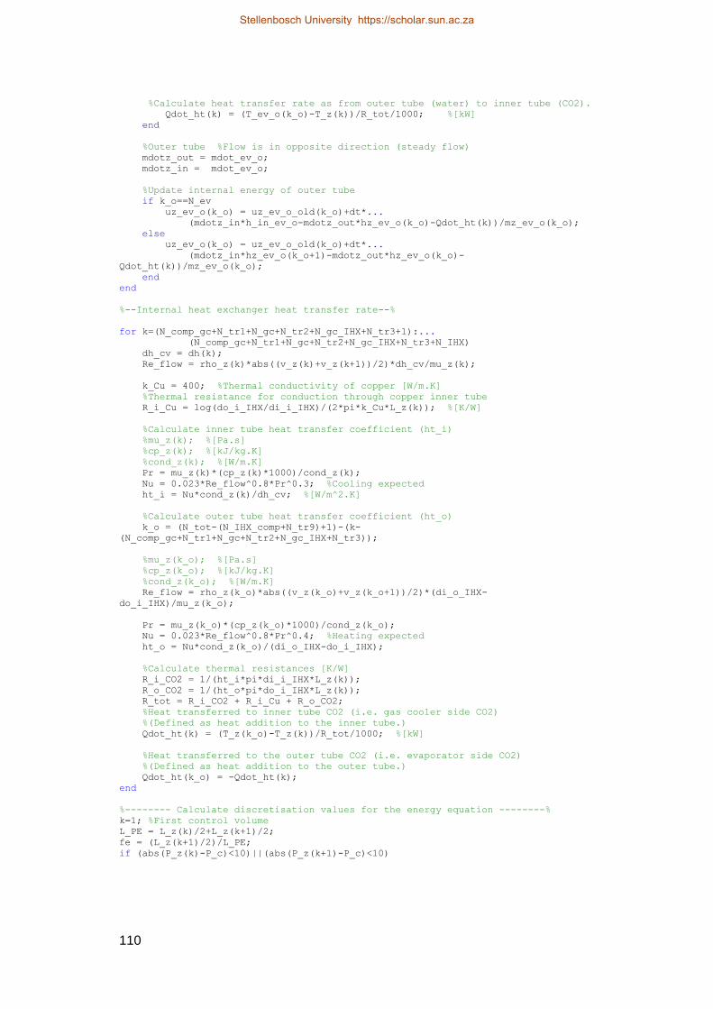
110

%Calculate heat transfer rate as from outer tube (water) to inner tube (CO2).

Qdot_ht(k) = (T_ev_o(k_o)-T_z(k))/R_tot/1000; %[kW]

end

%Outer tube %Flow is in opposite direction (steady flow)

mdotz_out = mdot_ev_o;

mdotz_in = mdot_ev_o;

%Update internal energy of outer tube

if k_o==N_ev

uz_ev_o(k_o) = uz_ev_o_old(k_o)+dt*...

(mdotz_in*h_in_ev_o-mdotz_out*hz_ev_o(k_o)-Qdot_ht(k))/mz_ev_o(k_o);

else

uz_ev_o(k_o) = uz_ev_o_old(k_o)+dt*...

(mdotz_in*hz_ev_o(k_o+1)-mdotz_out*hz_ev_o(k_o)-

Qdot_ht(k))/mz_ev_o(k_o);

end

end

%--Internal heat exchanger heat transfer rate--%

for k=(N_comp_gc+N_tr1+N_gc+N_tr2+N_gc_IHX+N_tr3+1):...

(N_comp_gc+N_tr1+N_gc+N_tr2+N_gc_IHX+N_tr3+N_IHX)

dh_cv = dh(k);

Re_flow = rho_z(k)*abs((v_z(k)+v_z(k+1))/2)*dh_cv/mu_z(k);



R_i_Cu = log(do_i_IHX/di_i_IHX)/(2*pi*k_Cu*L_z(k)); %[K/W]


%mu_z(k); %[Pa.s]




Nu = 0.023*Re_flow^0.8*Pr^0.3; %Cooling expected

ht_i = Nu*cond_z(k)/dh_cv; %[W/m^2.K]


k_o = (N_tot-(N_IHX_comp+N_tr9)+1)-(k-

(N_comp_gc+N_tr1+N_gc+N_tr2+N_gc_IHX+N_tr3));

%mu_z(k_o); %[Pa.s]

%cp_z(k_o); %[kJ/kg.K]

%cond_z(k_o); %[W/m.K]

Re_flow = rho_z(k_o)*abs((v_z(k_o)+v_z(k_o+1))/2)*(di_o_IHX-

do_i_IHX)/mu_z(k_o);

Pr = mu_z(k_o)*(cp_z(k_o)*1000)/cond_z(k_o);

Nu = 0.023*Re_flow^0.8*Pr^0.4; %Heating expected

ht_o = Nu*cond_z(k_o)/(di_o_IHX-do_i_IHX);


R_i_CO2 = 1/(ht_i*pi*di_i_IHX*L_z(k));

R_o_CO2 = 1/(ht_o*pi*do_i_IHX*L_z(k));


%Heat transferred to inner tube CO2 (i.e. gas cooler side CO2)

%(Defined as heat addition to the inner tube.)

Qdot_ht(k) = (T_z(k_o)-T_z(k))/R_tot/1000; %[kW]

%Heat transferred to the outer tube CO2 (i.e. evaporator side CO2)

%(Defined as heat addition to the outer tube.)

Qdot_ht(k_o) = -Qdot_ht(k);

end

%-------- Calculate discretisation values for the energy equation --------%

k=1; %First control volume

L_PE = L_z(k)/2+L_z(k+1)/2;

fe = (L_z(k+1)/2)/L_PE;

if (abs(P_z(k)-P_c)<10)||(abs(P_z(k+1)-P_c)<10)


111

cond_e = 0;

else

cond_e = fe*cond_z(k)+(1-fe)*cond_z(k+1);

end

%Axial heat conduction in the gas

Qdot_e = cond_e*A_v(k+1)*(T_z(k+1)-T_z(k))/(L_z(k)/2+L_z(k+1)/2)/1000; %[kW]

dh_cv = dh(k);


if Re_flow>2300 %flow assumed turbulent

Cf = 0.078*Re_flow^-0.25;

elseif Re_flow <= 1e-200 %if there is no flow then there is no friction

%(this prevents numerical errors)

Cf = 0;

else %flow assumed laminar

Cf = 16/Re_flow;

end

tau_x = 0.5*Cf*rho_z(k)*((v_z(k)+v_z(k+1))/2)^2;

F_w = 0; F_e = rho_e(k)*v_z(k+1)*A_v(k+1);

a_w(k) = 0; a_e(k) = max(0,-F_e);

a_p_old(k) = rho_z_old(k)*(A_v(k)+A_v(k+1))/2*L_z(k)/dt;

S_u(k) = -P_z(k)*(A_v(k+1)*v_z(k+1)-A_v(k)*v_z(k))+...

tau_x/1000*(pi*dh_cv*L_z(k))*abs(((v_z(k)+v_z(k+1))/2))+...

mdot_comp*u_out_comp+Qdot_ht(k)+a_p_old(k)*u_z_old(k)+Qdot_e;

a_p(k) = a_w(k)+a_e(k)+(F_e-F_w)+a_p_old(k)/rho_z_old(k)*rho_z(k);


dh_cv = dh(k);




rho_w = rho_e(k-1);

if (abs(P_z(k-1)-P_c)<10)||(abs(P_z(k)-P_c)<10) %Ignore axial conduction when

close to the critical pressure

cond_w = 0;

else

cond_w = fw*cond_z(k)+(1-fw)*cond_z(k-1);

end

if (abs(P_z(k)-P_c)<10)||(abs(P_z(k+1)-P_c)<10)

cond_e = 0;

else

cond_e = fe*cond_z(k)+(1-fe)*cond_z(k+1);

end

Qdot_e = cond_e*A_v(k+1)*(T_z(k+1)-T_z(k))/(L_z(k)/2+L_z(k+1)/2)/1000; %[kW]

Qdot_w = cond_w*A_v(k)*(T_z(k-1)-T_z(k))/(L_z(k-1)/2+L_z(k)/2)/1000; %[kW]

%Calculate skin friction factor for CO2 in current cv


Cf = 0.078*Re_flow^-0.25;


Cf = 0;


Cf = 16/Re_flow;

end


F_w = rho_w*v_z(k)*A_v(k); F_e = rho_e(k)*v_z(k+1)*A_v(k+1);

a_w(k) = max(F_w,0); a_e(k) = max(0,-F_e);


S_u(k) = -P_z(k)*(A_v(k+1)*v_z(k+1)-A_v(k)*v_z(k))+...

tau_x/1000*(pi*dh_cv*L_z(k))*abs(((v_z(k)+v_z(k+1))/2))+...

Qdot_ht(k)+a_p_old(k)*u_z_old(k)+Qdot_e+Qdot_w;

a_p(k) = a_w(k)+a_e(k)+F_e-F_w+a_p_old(k)/rho_z_old(k)*rho_z(k);

end

%Last control volume

k=N_tot;

L_WP = L_z(k-1)/2+L_z(k)/2;

fw = (L_z(k-1)/2)/L_WP;


112

rho_w = rho_e(k-1);

if (abs(P_z(k)-P_c)<10)||(abs(P_z(k-1)-P_c)<10)

cond_w = 0;

else

cond_w = fw*cond_z(k)+(1-fw)*cond_z(k-1);

end

Qdot_w = cond_w*A_v(k)*(T_z(k-1)-T_z(k))/(L_z(k-1)/2+L_z(k)/2)/1000; %[kW]

dh_cv = dh(k);

Re_flow = rho_z(k)*abs((v_z(k)+v_z(k+1))/2)*dh_cv/mu_z(k); %Use old velocity to

%approximate friction


Cf = 0.078*Re_flow^-0.25;


Cf = 0;


Cf = 16/Re_flow;

end


F_w = rho_w*v_z(k)*A_v(k);

F_e = 0;

a_w(k) = max(F_w,0); a_e(k) = 0;


S_u(k) = -P_z(k)*(A_v(k+1)*v_z(k+1)-A_v(k)*v_z(k))...

+tau_x/1000*(pi*dh_cv*L_z(k))*abs(((v_z(k)+v_z(k+1))/2))+...

-mdot_comp*u_z_old(k)+Qdot_ht(k)+a_p_old(k)*u_z_old(k)+Qdot_w;

a_p(k) = a_w(k)+a_e(k)+F_e-F_w+a_p_old(k)/rho_z_old(k)*rho_z(k);

%-------------------------------------------------------------------------%

%Check how well the internal energy currently satisfies the energy equation:

%Calculate specific internal energy residuals at each cv node

e_residual(1:N_tot) = 0;

k=1; %For first control volume

e_residual(k) = a_p(k)*u_z(k)-(a_e(k)*u_z(k+1)+S_u(k));

e_norm_factor(k) = a_p(k)*u_z(k);

for k=2:(N_tot-1) %Interior control volumes

e_residual(k) = a_p(k)*u_z(k)-(a_w(k)*u_z(k-1)+a_e(k)*u_z(k+1)+S_u(k));


end

k=N_tot; %For the last control volume

e_residual(k) = a_p(k)*u_z(k)-(a_w(k)*u_z(k-1)+S_u(k));


%Calculate sum of absolute specific internal energy residuals

sum_e_residuals = sum(abs(e_residual(:)));

sum_e_norm_factor = sum(abs(e_norm_factor(:)));

%This gives an indication of how well the energy equation is satisfied

norm_Global_e_Residual = sum_e_residuals/sum_e_norm_factor;

%-------------------------------------------------------------------------%

%TDMA solver for energy equation (calculate specific internal energy)

%-------------------------------------------------------------------------%

%alpha = a_e_c(k); %beta = a_w_c(k); %Dj = a_p_c(k);

%Boundary control volume

k=1;

Aj(k) = a_e(k)/(a_p(k)-0);

Cj_aks(k) = (0+S_u(k))/(a_p(k)-0);


Aj(k) = a_e(k)/(a_p(k)-a_w(k)*Aj(k-1));


end

k=N_tot; %Last control volume

Aj(k) = 0;


for k=N_tot:-1:1

if k==N_tot

u_z(k) = Cj_aks(k);


113

else

u_z(k) = Aj(k)*u_z(k+1)+Cj_aks(k);

end

end

%-------------------------------------------------------------------------%

%Update refrigerant side i.e. CO2 side

%Update pressure and other variables using equation of state P = f(rho,u)

for k=1:N_tot

%Recalculate properties only if one of the two variables has changed

%considerably i.e. changed more than 10^-7

if ((abs(rho_z(k)-rho_z_latest_upd(k))>10^-7)||(abs(u_z(k)-

u_z_latest_upd(k))>10^-7))

%Find properties at rho and u.

rho = rho_z(k); u = u_z(k);

T = T_z(k); %Use previous iteration’s value as initial guess

%If the flow is two-phase pre-assign initial guesses based on the

%previous iteration’s values.

rho_f = rho_f_z(k);

rho_g = rho_g_z(k);

alpha_vol = alpha_vol_z(k);

%Only use the following code if the program runs into an error with properties too

close to the critical region. It is rarely needed.

%If T>304.1281, and rho and u are in the two-phase region but very

%close to the critical point i.e. if they fall within the T=304.1281

%saturated lines then assign critical point values for other properties.

%{

if (((rho<468.2)&&(rho>467))&&...

((u>-1.904331870237819e+02)&&(u<1.901891527564772e+02)))&&

(abs(P_z(k)-P_c)<10)

%Assign critical point properties

T = T_c;

rho = rho_c;

CO2_Property

CO2_Conductivity;

Viscosity_CO2;

Two_ph = 0;

%Set i=2 so that new properties can be saved

i=2

else

%}

%Calculate properties

if P_z(k)>7390 %i.e. if previous pressure is above this level then

%expect it to remain single phase.


CO2_Conductivity;

Viscosity_CO2;

elseif (k>1)&&(k<N_tot)&&(xi_z(k-1)==xi_z(k+1))


CO2_Conductivity;

Viscosity_CO2;

elseif (k>1)&&(k<N_tot)&&(xi_z(k-1)>0)&&(xi_z(k-1)<1)&&...

(xi_z(k+1)>0)&&(xi_z(k+1)<1)

CO2_2Ph_Prop_at_rho_and_u








else

CO2_Prop_at_rho_and_u

end

%end

%Error prevention in case of wrong phase selection previously

if (Two_ph==0)&&((cp<0)||(isreal(cp)==0))%This occurs if the flow

%was incorrectly identified


114

%as single phase instead of two-phase

T=T_z(k);

rho=rho_z(k); u=u_z(k);









elseif ((Two_ph==1)&&((isreal(cp)==0))||(cp<0))

T=T_z(k);

rho=rho_z(k); u=u_z(k);


CO2_Conductivity;

Viscosity_CO2;

end

if i>1 %Only update properties if the first property iteration does not

%already satisfy the error margin.

%Store updated density and specific internal energy for use later

%in deciding if the properties need recalculating or not.

rho_z_latest_upd(k) = rho_z(k);

u_z_latest_upd(k) = u_z(k);

%Assign new properties

P_z(k) = P; T_z(k) = T; cp_z(k) = cp; cv_z(k) = cv; h_z(k) = h;

s_z(k) = s; cond_z(k) = cond; mu_z(k) = visc;

if Two_ph==1 %Update two-phase vectors

rho_f_z(k) = rho_f;

rho_g_z(k) = rho_g;

alpha_vol_z(k) = alpha_vol; xi_z(k) = xi;

else %Two_ph==0 thus flow is single phase

if rho>rho_c


else


end

end

end

end

end

%Update gas cooler outer tube side i.e. water side

%Calculate new properties for outer tube

for k=1:N_gc

%Recalculate properties only if the specific internal energy has

%changed considerably i.e. changed more than 10^-7

if (abs(uz_gc_o(k)-uz_gc_o_latest_upd(k))>10^-7)

u = uz_gc_o(k);

T = T_gc_o(k); %Use old value as initial guess

%Update to new values

uz_gc_o_latest_upd(k)=uz_gc_o(k);

T_gc_o(k) = T_w_at_u_f_func(u,T); %New temperature

hz_gc_o(k) = h_f_w_func(T_gc_o(k)); %New h

cpz_gc_o(k) = cp_f_w_func(T_gc_o(k)); %New cp

cond_gc_o(k) = cond_f_w_func(T_gc_o(k)); %New conductivity

mu_gc_o(k) = mu_f_w_func(T_gc_o(k)); %New viscosity

end

end

%Update evaporator outer tube side i.e. water side


for k=1:N_ev

%Recalculate properties only if the specific internal energy has

%changed considerably i.e. changed more than 10^-7

if (abs(uz_ev_o(k)-uz_ev_o_latest_upd(k))>10^-7)



115

u = uz_ev_o(k);

T = T_ev_o(k); %Use old value as initial guess

uz_ev_o_latest_upd(k) = uz_ev_o(k);

T_ev_o(k) = T_w_at_u_f_func(u,T); %New temperature

hz_ev_o(k) = h_f_w_func(T_ev_o(k)); %New h

cpz_ev_o(k) = cp_f_w_func(T_ev_o(k)); %New cp

cond_ev_o(k) = cond_f_w_func(T_ev_o(k)); %New conductivity

mu_ev_o(k) = mu_f_w_func(T_ev_o(k)); %New viscosity

end

end

%-------------------------------------------------------------------------%

%--Solve momentum equation to get new velocity field--%

%First momentum control volume

k=2;

%rho_w refers to the scalar control volume k and not the momentum control volume



rho_w = rho_e(k-1);

rho_p_old = (rho_z_old(k-1)+rho_z_old(k))/2; rho_p = (rho_z(k-1)+rho_z(k))/2;

a_p_old_mom(k) = rho_p_old*A_v(k)*(L_z(k-1)/2+L_z(k)/2)/dt;

F_w_mom = (mdot_comp+rho_w*v_z(k)*A_v(k))/2;

F_e_mom = (rho_w*v_z(k)*A_v(k)+rho_e(k)*v_z(k+1)*A_v(k+1))/2;

a_w_mom(k) = max(F_w_mom,0); a_e_mom(k) = max(0,-F_e_mom);

dh_cv = sqrt((dh(k-1)^2+dh(k)^2)/2);

Re_flow = (rho_z(k-1)+rho_z(k))/2*abs(v_z(k))*dh_cv/((mu_z(k-1)+mu_z(k))/2);


Cf = 0.078*Re_flow^-0.25;


Cf = 0;


Cf = 16/Re_flow;

end

tau_z = 0.5*Cf*rho_p*abs(v_z(k))*v_z(k);

S_u_mom(k) = (P_z(k-1)-P_z(k))*1000*A_v(k)-tau_z*pi*dh_cv*(L_z(k-

1)/2+L_z(k)/2)+a_p_old_mom(k)*v_z_old(k);

S_p_mom(k) = 0;%-0.5*Cf*rho_P*abs(v_z(k))*pi*(L_z(k-1)/2+L_z(k)/2)*dh_cv;

a_p_mom(k) = a_w_mom(k)+a_e_mom(k)+(F_e_mom-F_w_mom)-

S_p_mom(k)+a_p_old_mom(k)*rho_p/rho_p_old;

for k=3:N_tot-1 %For interior nodes (momentum control volumes)



rho_w = rho_e(k-1);

L_WWP = L_z(k-2)/2+L_z(k-1)/2; fww = (L_z(k-2)/2)/L_WP;

rho_ww = rho_e(k-2);



F_w_mom = (rho_ww*v_z(k-1)*A_v(k-1)+rho_w*v_z(k)*A_v(k))/2;

F_e_mom = (rho_w*v_z(k)*A_v(k)+rho_e(k)*v_z(k+1)*A_v(k+1))/2;


dh_cv = sqrt((dh(k-1)^2+dh(k)^2)/2);



Cf = 0.078*Re_flow^-0.25;


Cf = 0;


Cf = 16/Re_flow;

end






116



end

%Last momentum control volume

k=N_tot;


rho_w = rho_e(k-1);

L_WWP = L_z(k-2)/2+L_z(k-1)/2; fww = (L_z(k-2)/2)/L_WP;

rho_ww = rho_e(k-2);



F_w_mom = (rho_ww*v_z(k-1)*A_v(k-1)+rho_w*v_z(k)*A_v(k))/2;

F_e_mom = (rho_w*v_z(k)*A_v(k)+mdot_comp)/2;


dh_cv = sqrt((dh(k-1)^2+dh(k)^2)/2);



Cf = 0.078*Re_flow^-0.25;


Cf = 0;


Cf = 16/Re_flow;

end







%-------------------------------------------------------------------------%

%Check that the velocity used currently satisfies the momentum equation:

%Calculate momentum residuals at each velocity node

u_mom_residual(1:(N_tot+1)) = 0;

%For velocity node 1,i.e. k=1

k=1;

u_mom_residual(k) = a_p_mom(k)*v_z(k)-(a_e_mom(k)*v_z(k+1)+S_u_mom(k));

u_norm_factor(k) = a_p_mom(k)*v_z(k);

for k=2:(N_tot) %For interior control volumes

u_mom_residual(k) = a_p_mom(k)*v_z(k)-(a_w_mom(k)*v_z(k-

1)+a_e_mom(k)*v_z(k+1)+S_u_mom(k));


end

%For the last control volume

k=(N_tot+1);

u_mom_residual(k) = a_p_mom(k)*v_z(k)-(a_w_mom(k)*v_z(k-1)+S_u_mom(k));


%Calculate sum of absolute momentum residuals

sum_u_mom_residuals = sum(abs(u_mom_residual(:)));

sum_u_norm_factor = sum(abs(u_norm_factor(:)));

%This gives an indication of how well the momentum equation is satisfied

norm_Global_mom_Residual = sum_u_mom_residuals/sum_u_norm_factor

%-------------------------------------------------------------------------%

%Store velocity variable for use later in under-relaxation of velocity

v_z_interim = v_z;

%TDMA solver to calculate new velocities

%-------------------------------------------------------------------------%

%alpha = a_e(k); %beta = a_w(k); %Dj = a_p(k);

%Boundary conditions have velocities

k=1;

Aj_mom(k) = 0;

Cj_aks_mom(k) = v_in;

for k=2:N_tot %Interior control volumes

Aj_mom(k) = a_e_mom(k)/(a_p_mom(k)-a_w_mom(k)*Aj_mom(k-1));

Cj_aks_mom(k) = (a_w_mom(k)*Cj_aks_mom(k-1)+S_u_mom(k))/(a_p_mom(k)-

a_w_mom(k)*Aj_mom(k-1));

end

k=N_tot+1; %Last control volume


117

Aj_mom(k) = 0;

Cj_aks_mom(k) = v_out;

%Calculate new velocity from the discretised momentum equation

for k=(N_tot+1):-1:1

if k==(N_tot+1)

v_z(k) = Cj_aks_mom(k);

else

v_z(k) = Aj_mom(k)*v_z(k+1)+Cj_aks_mom(k);

end

end

%Take the new velocity as a weighted average between the previously used

%velocity and the newly calculated velocity

alpha_v_z = 0.050;

v_z = (1-alpha_v_z)*v_z_interim+alpha_v_z*v_z;

%-------------------------------------------------------------------------%

end %End of while loop

APPENDIX D: COMPRESSOR PRODUCT DATA

The Embraco EK6210CD compressor is selected for this project. Product data

below shows that the rated cooling load at -10 is 700 W.

Figure D1: EK6210CD product data


118

APPENDIX E: STEADY-STATE CAPILLARY TUBE SIMULATION MODEL

%Capillary_Tube.m is a script file containing a steady-state model for the

%capillary tube. It is used to determine the steady-state mass flow rate for a

%particular capilaary tube design and operating conditions.

%----------------- Expansion device modelling (State 3-4) ----------------%

% Expansion device is a capillary tube

l_ct = 3.5; %Length of capillary tube [m] d_ct = 0.00079; %Diameter of capillary tube [m]

mdot_cap = 1*10^-16; %Initialise mass flow rate through capillary tube [kg/s]

%Define lower bound for mass flow rate

xj(1) = mdot_cap; %Mass flow rate through capillary tube [kg/s]

Pct_in = 8500; %Pressure at inlet of capillary tube [kPa]

Tct_in = 32+273.15; %Inlet temperature of capillary tube [K]

Pct_out= 2648.677254832481; %Pressure at outlet of capillary tube (Psat_ev) [kPa]

P=Pct_in; T=Tct_in; CO2_1Ph_Prop_at_P_and_T;

h_ct = h; %Assume stays constant for the capillary tube

%Determine pressure at which flow becomes two-phase (i.e. crosses the saturation

line)

hsat = h_ct;

if (hsat<h_fi(length(h_fi))), P_sat_cross = interp1(h_fi,Pi,hsat);

elseif (hsat>h_gi_1(length(h_gi_1))), P_sat_cross = interp1(h_gi_1,Pi_1,hsat);

end

%Can calculate the actual crossing if interpolation is not good enough

%CO2_Sat_Prop_at_hsat

%P_sat_cross = P;

Ac_ct = pi/4*d_ct^2; %Area of capillary tube [m]

%--Determine regions of single and two-phase flow in the capillary tube.--%

if (Pct_in>=P_sat_cross)&&(Pct_out>=P_sat_cross) %Flow is single phase only

Scenario = 1;

N_ct_1ph = 200; %Number of control volumes for the single phase flow

%in the capillary tube.

dP_ct_k_1ph = (Pct_in-Pct_out)/(N_ct_1ph);

elseif (Pct_in>=P_sat_cross)&&(Pct_out<P_sat_cross)

%Flow is single phase at the start and changes to two phase flow downstream

Scenario = 2;

N_ct_1ph = 200; %Number of control volumes for the single phase flow


dP_ct_k_1ph = (Pct_in-P_sat_cross)/(N_ct_1ph);

N_ct_2ph = 500; %Number of control volumes for the two phase flow


dP_ct_k_2ph = (P_sat_cross-Pct_out)/(N_ct_2ph);

else %Flow is two-phase only

Scenario = 3;

N_ct_2ph = 500; %Number of control volumes for the two phase flow


dP_ct_k_2ph = (Pct_in-Pct_out)/(N_ct_2ph);

end %end if

%Calculate properties of the flow

if (Scenario == 1)||(Scenario == 2)

for k=1:N_ct_1ph

if k==1

Pct(k)=Pct_in-dP_ct_k_1ph/2;

else

Pct(k)=Pct(k-1)-dP_ct_k_1ph;

end

if k==1 %Inlet conditions of 1st control volume

P = Pct(k)+dP_ct_k_1ph/2; h=h_ct; CO2_1Ph_Prop_at_P_and_h;

rho_in_1ph(k) = rho;

else %Inlet conditions of k'th control volume

rho_in_1ph(k) = rho_out_1ph(k-1);


119

end

%Determine rho and viscosity of the k'th control volume

P = Pct(k); h = h_ct; CO2_1Ph_Prop_at_P_and_h;

rho_1ph(k)=rho;

Viscosity_CO2 %Determine the viscosity at T and rho

visc_1ph(k) = visc;

%Outlet conditions of k'th control volume

rho_out_1ph(k) = 2*rho_1ph(k)-rho_in_1ph(k); %Approximation to save computation

%time

end %end for loop

end %end if

if (Scenario == 2)||(Scenario==3)

for k=1:N_ct_2ph

if k==1

if Scenario==2, Pct(k)=P_sat_cross-dP_ct_k_2ph/2;

else Pct(k)=Pct_in-dP_ct_k_2ph/2;

end

else

Pct(k)=Pct(k-1)-dP_ct_k_2ph;

end

if k==1 %Inlet conditions of 1st control volume

P = Pct(k)+dP_ct_k_2ph/2; h = h_ct; CO2_2Ph_Prop_at_P_and_h;

rho_in_2ph(k) = rho;

else %Inlet conditions of k'th control volume

rho_in_2ph(k) = rho_out_2ph(k-1);

end

%Determine rho and viscosity of the k'th control volume

P = Pct(k); h = h_ct; CO2_2Ph_Prop_at_P_and_h;

rho_2ph(k)= rho; %Homogenous density

rho_f_2ph(k) = rho_f;

%Determine gas viscosity


%Determine fluid viscosity


%Determine the homogenous mixture's viscosity

visc_2ph(k) = 1/(xi/visc_g+(1-xi)/visc_f);

visc_f_2ph(k) = visc_f; %Fluid viscosity

%Outlet conditions of k'th control volume

rho_out_2ph(k) = 2*rho_2ph(k)-rho_in_2ph(k); %Approximation to save computation

time

end %end for loop

end %end if

p=0;

%Initialise length parameter for itteration

Length = l_ct*2;

%Define upper bound for mass flow rate

mdot_cap = 0.2; %Mass flow rate through capillary tube [kg/s]

xj(2) = mdot_cap;

while (abs(Length-l_ct)>10^-6)&&(p<1000)

p=p+1;

for j=1:3

if j==3, xj(3)=(xj(1)+xj(2))/2; end %Define mid value for mass flow rate

mdot_cap = xj(j);

%Calculate pressure drop length of the single phase flow region


for k=1:N_ct_1ph

Re_ct = mdot_cap*d_ct/(visc_1ph(k)*Ac_ct);

if Re_ct>2300

Cf = 0.078*Re_ct^-0.25;

else

Cf = 16/Re_ct;

end

L_1ph(k)=(dP_ct_k_1ph*1000-(mdot_cap/Ac_ct)^2*(1/rho_out_1ph(k)-...

1/rho_in_1ph(k)))*(0.5*rho_1ph(k)*d_ct/(Cf*(mdot_cap/Ac_ct)^2));

end %end for-loop


120

end %end if

%Calculate pressure drop length of the two-phase flow region


for k=1:N_ct_2ph

%Determine Reynolds number based on liquid only (lo)

Re_ct_lo = mdot_cap*d_ct/(visc_f_2ph(k)*Ac_ct);

if Re_ct_lo>2300, Cf_lo = 0.078*Re_ct_lo^-0.25;

else Cf_lo = 16/Re_ct_lo;

end

%Determine Reynolds number of homogenous flow

Re_ct_h = mdot_cap*d_ct/(visc_2ph(k)*Ac_ct);

if Re_ct_h>2300, Cf_h = 0.078*Re_ct_h^-0.25;

else Cf_h = 16/Re_ct_h;

end

%Determine two-phase flow friction multiplier

Phi_2ph_fr = (Cf_h/Cf_lo)*(rho_f_2ph(k)/rho_2ph(k));

L_2ph(k)=(dP_ct_k_2ph*1000-(mdot_cap/Ac_ct)^2*(1/rho_out_2ph(k)-...

1/rho_in_2ph(k)))*(0.5*rho_2ph(k)*d_ct/...

(Cf_lo*Phi_2ph_fr*(mdot_cap/Ac_ct)^2));

end %end for-loop

end %end if

end %end for j=1:3 for-loop

%Initialise variable

Negative = 0;

%Calculate pressure drop length of the different scenario's

if Scenario==1, Length = sum(L_1ph);

for k=1:N_ct_1ph

if L_1ph(k)<0, Negative = 1; end

end

elseif Scenario==2, Length = sum(L_1ph)+sum(L_2ph);

for k=1:N_ct_1ph


end

for k=1:N_ct_2ph


end

elseif Scenario==3, Length = sum(L_2ph);

for k=1:N_ct_2ph


end

end

%Perform interval halving

if Negative==1, xj(2) = xj(3); %Decrease mass flow rate

else

if Length<=l_ct, xj(2) = xj(3); %Decrease mass flow rate

else xj(1) = xj(3); %Increase mass flow rate

end

end

end

mdot_cap = (xj(1)+xj(2))/2 %Output mass flow rate [kg/s]


121

APPENDIX F: THERMOCOUPLE CALIBRATION

The table below shows the calibration equations for the 20 T-type thermocouples

used in the experimental setup of the refrigeration system built. is the true

temperature (or adjusted temperature) and is the measured temperature.

Table F1: Thermocouple calibration equations

Thermocouple

number

Calibration equation

( )

Correlation

coefficient (R2)

1 0.99999841

2 0.99999932

3 0.99999925

4 0.99999972

5 0.99999691

6 0.99999027

7 0.99999359

8 0.99999086

9 0.99999372

10 0.99999861

11 0.99999795

12 0.99999929

13 0.99999927

14 0.99999913

15 0.99999573

16 0.99999312

17 0.99999183

18 0.99999110

19 0.99999170

20 0.99999817


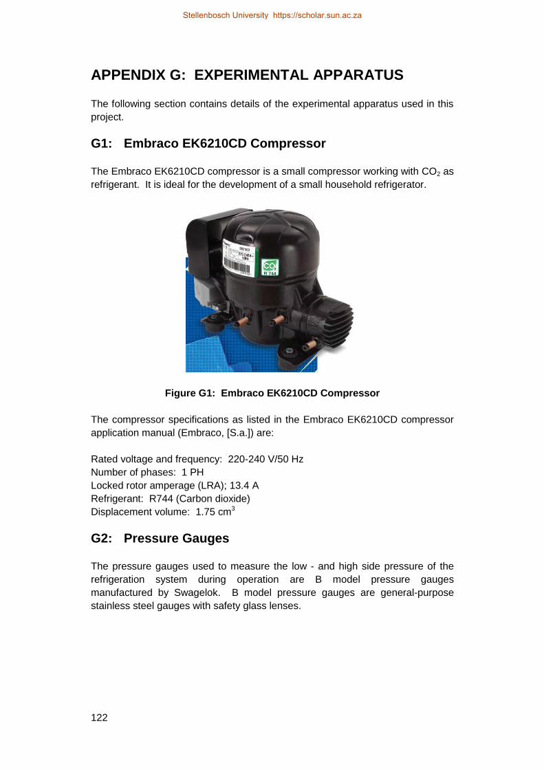
122

APPENDIX G: EXPERIMENTAL APPARATUS

The following section contains details of the experimental apparatus used in this

project.

G1: Embraco EK6210CD Compressor

The Embraco EK6210CD compressor is a small compressor working with CO2 as

refrigerant. It is ideal for the development of a small household refrigerator.

Figure G1: Embraco EK6210CD Compressor

The compressor specifications as listed in the Embraco EK6210CD compressor

application manual (Embraco, [S.a.]) are:

Rated voltage and frequency: 220-240 V/50 Hz

Number of phases: 1 PH

Locked rotor amperage (LRA); 13.4 A

Refrigerant: R744 (Carbon dioxide)

Displacement volume: 1.75 cm3

G2: Pressure Gauges

The pressure gauges used to measure the low - and high side pressure of the

refrigeration system during operation are B model pressure gauges

manufactured by Swagelok. B model pressure gauges are general-purpose

stainless steel gauges with safety glass lenses.


123

Figure G2: Swagelok pressure gauges

The pressure gauge specifications as listed in the product data sheet are:

LP pressure gauge model designator: PGI-63B-BG100-LAQX

HP pressure gauge model designator: PGI-63B-BG250-LAQX

HP pressure gauge range: 0 to 250 bar

LP pressure gauge range: 0 to 100 bar

Type: Positive-pressure gauge

Dial size: 63 mm

Model: B

End Connection: 1/4”

Accuracy: 1.5 % of span

Weather protection: Weather-tight (NEMA 4X/IP65)

Ambient operating temperature (unfilled): -40 to 60

Media operating temperature (unfilled): 200 maximum

Temperature error: 0.4 % for every 10 temperature change from 20

G3: B.I.C.I.SA-5500 Water Pump

The B.I.C.I.SA-5500 is a submersible water pump used for aquarium water

circulation.

Figure G3: B.I.C.I.SA-5500 water pump

LP Pressure

gauge

HP Pressure

gauge


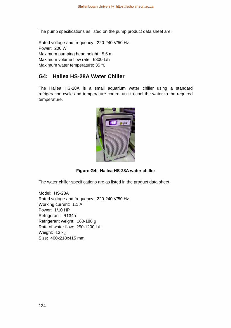
124

The pump specifications as listed on the pump product data sheet are:


Power: 200 W

Maximum pumping head height: 5.5 m

Maximum volume flow rate: 6800 L/h

Maximum water temperature: 35

G4: Hailea HS-28A Water Chiller

The Hailea HS-28A is a small aquarium water chiller using a standard

refrigeration cycle and temperature control unit to cool the water to the required

temperature.

Figure G4: Hailea HS-28A water chiller

The water chiller specifications are as listed in the product data sheet:

Model: HS-28A


Working current: 1.1 A

Power: 1/10 HP

Refrigerant: R134a

Refrigerant weight: 160-180

Rate of water flow: 250-1200 L/h

Weight: 13 k

Size: 400x218x415 mm


125

G5: Agilent 34970A Data Acquisition/Data Logger Switch Unit

The Agilent 34970A Data Acquisition/Data Logger Switch Unit is now

manufactured by Keysight Technologies. It contains a built-in 6 1/2 digit digital

multimeter capable of measuring 250 channels per second. It has a 3-slot

mainframe, thus allowing 60 2-wire measurements (20 per slot). On-module

screw-terminal connections are used to connect the various measuring probes.

Figure G5: Agilent 34970A Data Acquisition/Switch Unit

The Agilent 34970A Data Acquisition/Data Logger Switch Unit specifications as

obtained from Keysight Technologies (2015) are:

3-slot mainframe with built-in GPIB and RS232 interfaces

6 1/2-digit (22-bit) internal DMM, with scanning up to 250 channels per second

8 switch and control plug-in modules to choose from

Built-in signal conditioning measures thermocouples, thermistors and RTDs,

ac/dc volts and current, frequency and period, resistance

50k readings of non-volatile memory holds data when power is removed

Hi/Lo alarm limits on each channel, plus 4 TTL alarm outputs

Free Benchlink data logger software to create tests without programming

A 34901A plug-in module was used with the data logger. This module provides

20 two-wire channels and has a built-in thermocouple reference.


126

G6: Efergy Energy Monitoring Socket

The efergy energy monitoring socket measures the energy efficiency of any

appliance plugged into it. It is used in this project to measure the compressor

power consumption.

Figure G6: Efergy energy monitoring socket

The specifications of the efergy energy monitoring socket as given by the product

data sheet are:

Model name: Energy Monitoring Socket

Model number: EMS-RSA

Operating voltage: 230 V

Operating current: 16A max.

Working voltage: 170 V-276 V

Accuracy: 2 %

Measuring Features: Watt( W), Kilowatt Hours (kWh), Voltage (V), Current (A),

Frequency (Hz), Power Factor (%), Max. Watts (W)

Also: Measures time on, and cost if electricity tariff is programmed into it.

Display range: Time (0s-9999 days), Power (0 W-9999 W), Energy (0-

9999 kWh),

Voltage (0-9999 V), Current (0.000-16.00 A),

Frequency (0.000-9999 Hz), Price (00.00-99.99 R)


Transient Simulation of a Sub- to Transcritical C0 ...

Documents

Transcript of Transient Simulation of a Sub- to Transcritical C0 ...